Fatigue Predictions using Statistical Inference within the Monitas II Project Frank van der Meulen (1) , Remco Hageman (2) (1) Delft Institute of Applied Mathematics, Delft University of Technology, Delft, The Netherlands (2) Hydro-Structural Services, MARIN, Wageningen, The Netherlands ABSTRACT In this paper a statistical method is described for predicting fatigue accumulation. The proposed method for predicting accumulated fatigue is based on a nonparametric Bayesian analysis. Bayesian analysis provides a natural prediction framework for combining long-term design information and actual measured data. This work is part of the Monitas II project which delivered an advisory hull monitoring system for FPSOs with automatic data analyses capabilities. The prediction tool is to be embedded in this hull monitoring system. KEY WORDS: Dirichlet process prior; Bayesian Statistics; fatigue; FPSO; Monitoring. INTRODUCTION In 2010 the Monitas Joint Industry Project (JIP) has concluded (L’Hostis, Kaminski and Aalberts, 2010). The Monitas JIP delivered an automated measurement system and data analysis procedure to monitor the fatigue lifetime consumption of FPSO hulls. This system is called Monitas, which stands for Monitoring Advisory System. The system is capable of monitoring fatigue lifetime consumption. Furthermore, if the fatigue lifetime is consumed faster or slower in comparison with design calculations, Monitas can explain why. The Monitas methodology is discussed in more detail by L’Hostis, van der Cammen, Hageman and Aalberts (2012). At the end of the Monitas JIP the project partners decided to prolong the Project and continue improving the Monitas system. This paper will describe the efforts regarding fatigue prediction that have been executed for the Monitas II JIP. Execution of fatigue prediction is useful for two purposes. The first purpose is to develop an Inspection, Repair and Maintenance (IRM) schedule that uses monitoring data to determine rational inspection intervals. Risk Based Inspection (RBI) is an inspection methodology that relies strongly on in-depth structural analysis to determine optimal inspection intervals and scope. The coupling between monitoring systems and an RBI regime is discussed by Tammer and Kaminski (2012). The second purpose is to justify lifetime extension of FPSOs. An FPSO that has been continuously monitored and for which fatigue predictions can be executed in a consistent way gives an operator better insights in possibilities for lifetime extension. The goal of fatigue predictions is to obtain upper and lower prediction bounds for the fatigue accumulation during future operations of an FPSO. These predictions ought to employ both the long-term design information and the actual measured data to make optimal use of the measurement system. This paper presents a statistical method for making such predictions together with some results that have been obtained with this method. In the first part of this paper an exploratory analysis of the data is executed and the fatigue design procedure is addressed. The theoretical background of the proposed statistical methods is discussed next. Finally, some results of the fatigue forecasts are shown. AVAILABLE DATA The analysis presented in this paper is based on data of a Gulf of Guinea FPSO, hereafter referred to as GoG FPSO. A systematic analysis procedure for this FPSO has been developed within the Monitas II project, see L’Hostis, van der Cammen, Hageman and Aalberts (2012). The GoG FPSO has been producing since March 2012. All analyses in this paper are based on 6 months of data, from March up to August 2012. During the design of this FPSO a set of environmental and operational conditions has been used. These conditions are referred to as design data and include wave characteristics and load cases. The waves have been subdivided into swell and wind-induced waves. The waves have been modeled using a JONSWAP spectrum and a spreading function of the type . The JONSWAP parameter γ and the spreading parameter which describe windsea and swell are shown in Table 1. The scatter diagram of swell is depicted in Fig. 1. The assumed distribution of load cases is shown in Table 2.
Transcript
Fatigue Predictions using Statistical Inference within the Monitas II Project
Frank van der Meulen(1)
, Remco Hageman(2)
(1) Delft Institute of Applied Mathematics, Delft University of Technology, Delft, The Netherlands
(2) Hydro-Structural Services, MARIN, Wageningen, The Netherlands
ABSTRACT
In this paper a statistical method is described for predicting fatigue
accumulation. The proposed method for predicting accumulated fatigue
is based on a nonparametric Bayesian analysis. Bayesian analysis
provides a natural prediction framework for combining long-term
design information and actual measured data. This work is part of the
Monitas II project which delivered an advisory hull monitoring system
for FPSOs with automatic data analyses capabilities. The prediction
tool is to be embedded in this hull monitoring system.
KEY WORDS: Dirichlet process prior; Bayesian Statistics; fatigue;
FPSO; Monitoring.
INTRODUCTION
In 2010 the Monitas Joint Industry Project (JIP) has concluded
(L’Hostis, Kaminski and Aalberts, 2010). The Monitas JIP delivered an
automated measurement system and data analysis procedure to monitor
the fatigue lifetime consumption of FPSO hulls. This system is called
Monitas, which stands for Monitoring Advisory System. The system is
capable of monitoring fatigue lifetime consumption. Furthermore, if the
fatigue lifetime is consumed faster or slower in comparison with design
calculations, Monitas can explain why. The Monitas methodology is
discussed in more detail by L’Hostis, van der Cammen, Hageman and
Aalberts (2012).
At the end of the Monitas JIP the project partners decided to prolong
the Project and continue improving the Monitas system. This paper will
describe the efforts regarding fatigue prediction that have been
executed for the Monitas II JIP.
Execution of fatigue prediction is useful for two purposes. The first
purpose is to develop an Inspection, Repair and Maintenance (IRM)
schedule that uses monitoring data to determine rational inspection
intervals. Risk Based Inspection (RBI) is an inspection methodology
that relies strongly on in-depth structural analysis to determine optimal
inspection intervals and scope. The coupling between monitoring
systems and an RBI regime is discussed by Tammer and Kaminski
(2012). The second purpose is to justify lifetime extension of FPSOs.
An FPSO that has been continuously monitored and for which fatigue
predictions can be executed in a consistent way gives an operator better
insights in possibilities for lifetime extension.
The goal of fatigue predictions is to obtain upper and lower prediction
bounds for the fatigue accumulation during future operations of an
FPSO. These predictions ought to employ both the long-term design
information and the actual measured data to make optimal use of the
measurement system. This paper presents a statistical method for
making such predictions together with some results that have been
obtained with this method.
In the first part of this paper an exploratory analysis of the data is
executed and the fatigue design procedure is addressed. The theoretical
background of the proposed statistical methods is discussed next.
Finally, some results of the fatigue forecasts are shown.
AVAILABLE DATA
The analysis presented in this paper is based on data of a Gulf of
Guinea FPSO, hereafter referred to as GoG FPSO. A systematic
analysis procedure for this FPSO has been developed within the
Monitas II project, see L’Hostis, van der Cammen, Hageman and
Aalberts (2012). The GoG FPSO has been producing since March
2012. All analyses in this paper are based on 6 months of data, from
March up to August 2012.
During the design of this FPSO a set of environmental and operational
conditions has been used. These conditions are referred to as design
data and include wave characteristics and load cases. The waves have
been subdivided into swell and wind-induced waves. The waves have
been modeled using a JONSWAP spectrum and a spreading function of
the type . The JONSWAP parameter γ and the spreading
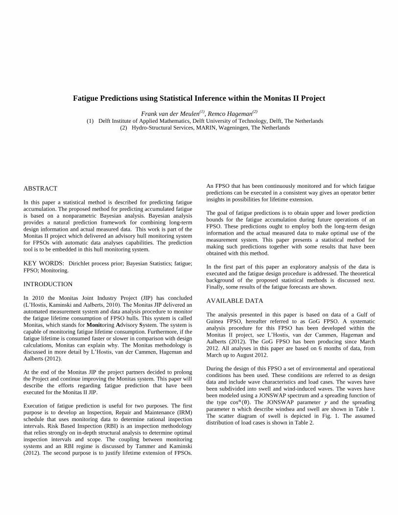
parameter which describe windsea and swell are shown in Table 1.
The scatter diagram of swell is depicted in Fig. 1. The assumed
distribution of load cases is shown in Table 2.
Table 1: Wave description parameters
Windsea Swell
γ 2.2 3.3
3 8
Fig. 1: Design scatter diagram for swell
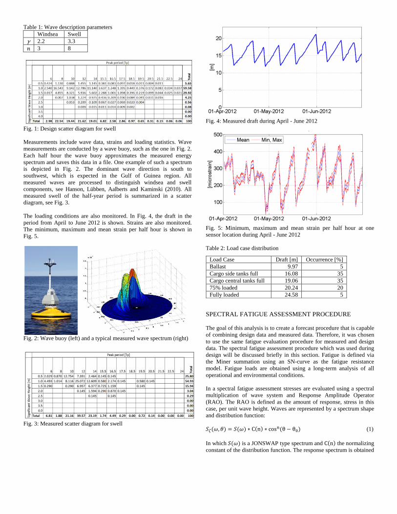
Measurements include wave data, strains and loading statistics. Wave
measurements are conducted by a wave buoy, such as the one in Fig. 2.
Each half hour the wave buoy approximates the measured energy
spectrum and saves this data in a file. One example of such a spectrum
is depicted in Fig. 2. The dominant wave direction is south to
southwest, which is expected in the Gulf of Guinea region. All
measured waves are processed to distinguish windsea and swell
components, see Hanson, Lübben, Aalberts and Kaminski (2010). All
measured swell of the half-year period is summarized in a scatter
diagram, see Fig. 3.
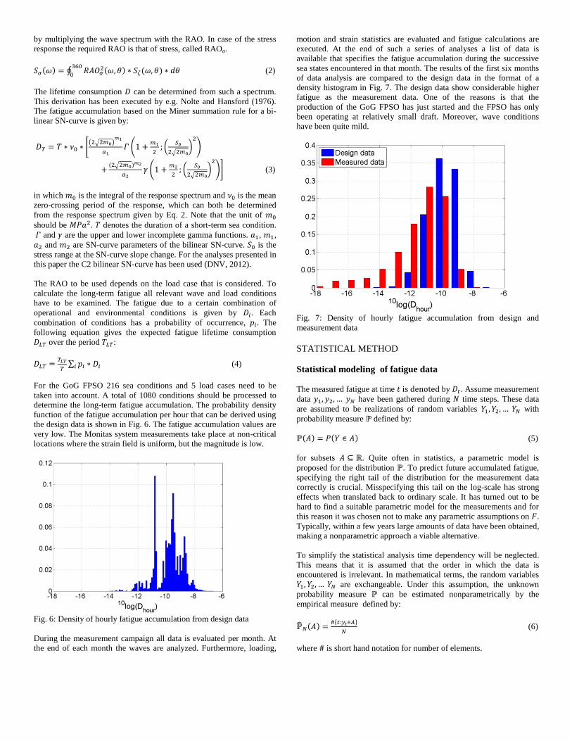
The loading conditions are also monitored. In Fig. 4, the draft in the
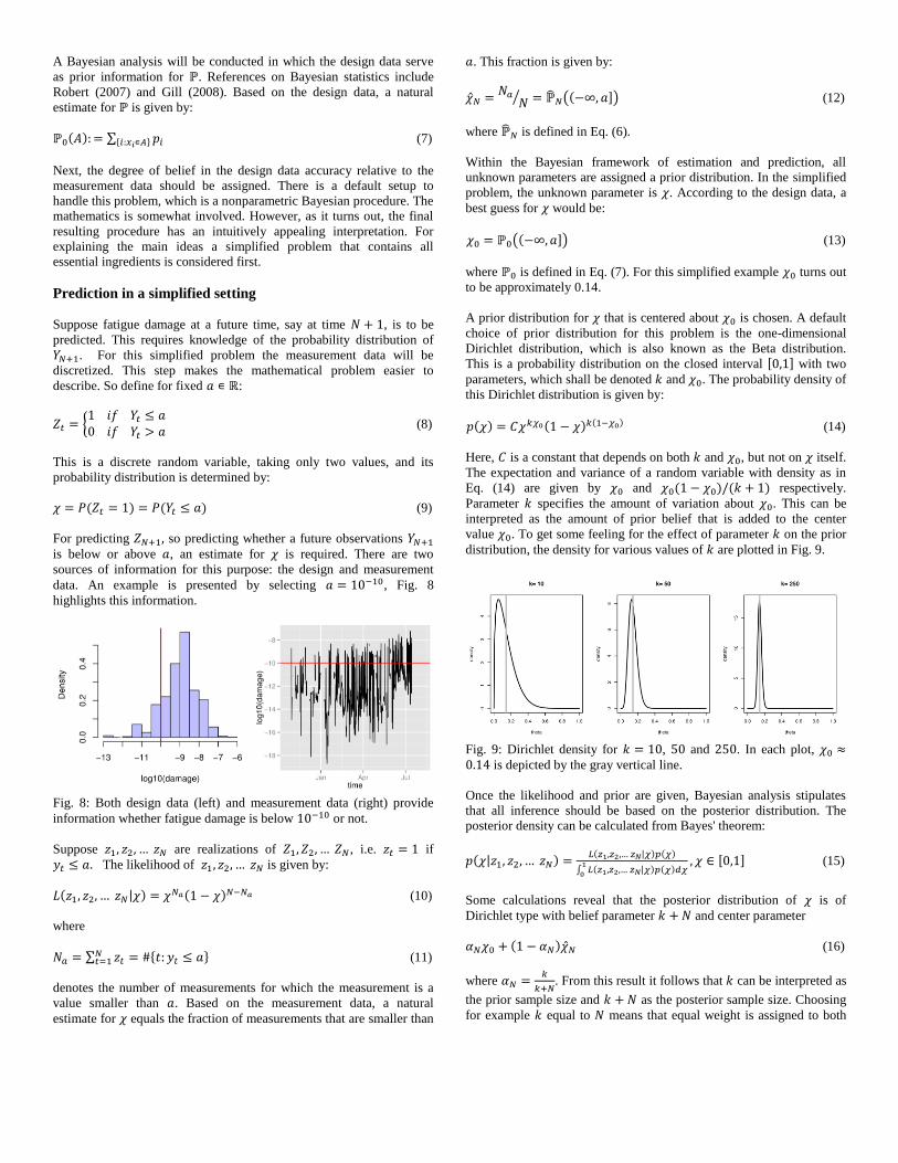
period from April to June 2012 is shown. Strains are also monitored.
The minimum, maximum and mean strain per half hour is shown in
Fig. 5.
Fig. 2: Wave buoy (left) and a typical measured wave spectrum (right)
Fig. 3: Measured scatter diagram for swell
Fig. 4: Measured draft during April - June 2012
Fig. 5: Minimum, maximum and mean strain per half hour at one
sensor location during April - June 2012
Table 2: Load case distribution
SPECTRAL FATIGUE ASSESSMENT PROCEDURE
The goal of this analysis is to create a forecast procedure that is capable
of combining design data and measured data. Therefore, it was chosen
to use the same fatigue evaluation procedure for measured and design
data. The spectral fatigue assessment procedure which was used during
design will be discussed briefly in this section. Fatigue is defined via
the Miner summation using an SN-curve as the fatigue resistance
model. Fatigue loads are obtained using a long-term analysis of all
operational and environmental conditions.
In a spectral fatigue assessment stresses are evaluated using a spectral
multiplication of wave system and Response Amplitude Operator
(RAO). The RAO is defined as the amount of response, stress in this
case, per unit wave height. Waves are represented by a spectrum shape
and distribution function:
(1)
In which is a JONSWAP type spectrum and the normalizing
constant of the distribution function. The response spectrum is obtained
Load Case Draft [m] Occurrence [%]
Ballast 9.97 5
Cargo side tanks full 16.08 35
Cargo central tanks full 19.06 35
75% loaded 20.24 20
Fully loaded 24.58 5
by multiplying the wave spectrum with the RAO. In case of the stress
response the required RAO is that of stress, called RAOσ.
(2)
The lifetime consumption can be determined from such a spectrum.
This derivation has been executed by e.g. Nolte and Hansford (1976).
The fatigue accumulation based on the Miner summation rule for a bi-
linear SN-curve is given by:
(3)
in which is the integral of the response spectrum and is the mean
zero-crossing period of the response, which can both be determined
from the response spectrum given by Eq. 2. Note that the unit of
should be . denotes the duration of a short-term sea condition.
and are the upper and lower incomplete gamma functions. , ,
and are SN-curve parameters of the bilinear SN-curve. is the
stress range at the SN-curve slope change. For the analyses presented in
this paper the C2 bilinear SN-curve has been used (DNV, 2012).
The RAO to be used depends on the load case that is considered. To
calculate the long-term fatigue all relevant wave and load conditions
have to be examined. The fatigue due to a certain combination of
operational and environmental conditions is given by . Each
combination of conditions has a probability of occurrence, . The
following equation gives the expected fatigue lifetime consumption
over the period :
(4)
For the GoG FPSO 216 sea conditions and 5 load cases need to be
taken into account. A total of 1080 conditions should be processed to
determine the long-term fatigue accumulation. The probability density
function of the fatigue accumulation per hour that can be derived using
the design data is shown in Fig. 6. The fatigue accumulation values are
very low. The Monitas system measurements take place at non-critical
locations where the strain field is uniform, but the magnitude is low.
Fig. 6: Density of hourly fatigue accumulation from design data
During the measurement campaign all data is evaluated per month. At
the end of each month the waves are analyzed. Furthermore, loading,
motion and strain statistics are evaluated and fatigue calculations are
executed. At the end of such a series of analyses a list of data is
available that specifies the fatigue accumulation during the successive
sea states encountered in that month. The results of the first six months
of data analysis are compared to the design data in the format of a
density histogram in Fig. 7. The design data show considerable higher
fatigue as the measurement data. One of the reasons is that the
production of the GoG FPSO has just started and the FPSO has only
been operating at relatively small draft. Moreover, wave conditions
have been quite mild.
Fig. 7: Density of hourly fatigue accumulation from design and
measurement data
STATISTICAL METHOD
Statistical modeling of fatigue data
The measured fatigue at time is denoted by . Assume measurement
data have been gathered during time steps. These data
are assumed to be realizations of random variables with
probability measure defined by:
(5)
for subsets . Quite often in statistics, a parametric model is
proposed for the distribution . To predict future accumulated fatigue,
specifying the right tail of the distribution for the measurement data
correctly is crucial. Misspecifying this tail on the log-scale has strong
effects when translated back to ordinary scale. It has turned out to be
hard to find a suitable parametric model for the measurements and for
this reason it was chosen not to make any parametric assumptions on .
Typically, within a few years large amounts of data have been obtained,
making a nonparametric approach a viable alternative.
To simplify the statistical analysis time dependency will be neglected.
This means that it is assumed that the order in which the data is
encountered is irrelevant. In mathematical terms, the random variables
are exchangeable. Under this assumption, the unknown
probability measure can be estimated nonparametrically by the
empirical measure defined by:
(6)
where is short hand notation for number of elements.
A Bayesian analysis will be conducted in which the design data serve
as prior information for . References on Bayesian statistics include
Robert (2007) and Gill (2008). Based on the design data, a natural
estimate for is given by:
(7)
Next, the degree of belief in the design data accuracy relative to the
measurement data should be assigned. There is a default setup to
handle this problem, which is a nonparametric Bayesian procedure. The
mathematics is somewhat involved. However, as it turns out, the final
resulting procedure has an intuitively appealing interpretation. For
explaining the main ideas a simplified problem that contains all
essential ingredients is considered first.
Prediction in a simplified setting
Suppose fatigue damage at a future time, say at time , is to be
predicted. This requires knowledge of the probability distribution of
. For this simplified problem the measurement data will be
discretized. This step makes the mathematical problem easier to
describe. So define for fixed :
(8)
This is a discrete random variable, taking only two values, and its
probability distribution is determined by:
(9)
For predicting , so predicting whether a future observations is below or above , an estimate for is required. There are two
sources of information for this purpose: the design and measurement
data. An example is presented by selecting , Fig. 8
highlights this information.
Fig. 8: Both design data (left) and measurement data (right) provide
information whether fatigue damage is below or not.
Suppose are realizations of , i.e. if
The likelihood of is given by:
(10)
where
(11)
denotes the number of measurements for which the measurement is a
value smaller than . Based on the measurement data, a natural
estimate for equals the fraction of measurements that are smaller than
. This fraction is given by:
(12)
where is defined in Eq. (6).
Within the Bayesian framework of estimation and prediction, all
unknown parameters are assigned a prior distribution. In the simplified
problem, the unknown parameter is . According to the design data, a
best guess for would be:
(13)
where is defined in Eq. (7). For this simplified example turns out
to be approximately 0.14.
A prior distribution for that is centered about is chosen. A default
choice of prior distribution for this problem is the one-dimensional
Dirichlet distribution, which is also known as the Beta distribution.
This is a probability distribution on the closed interval with two
parameters, which shall be denoted and . The probability density of
this Dirichlet distribution is given by:
(14)
Here, is a constant that depends on both and , but not on itself.
The expectation and variance of a random variable with density as in
Eq. (14) are given by and respectively.
Parameter specifies the amount of variation about . This can be
interpreted as the amount of prior belief that is added to the center
value . To get some feeling for the effect of parameter on the prior
distribution, the density for various values of are plotted in Fig. 9.
Fig. 9: Dirichlet density for , and . In each plot, is depicted by the gray vertical line.
Once the likelihood and prior are given, Bayesian analysis stipulates
that all inference should be based on the posterior distribution. The
posterior density can be calculated from Bayes' theorem:
(15)
Some calculations reveal that the posterior distribution of is of
Dirichlet type with belief parameter and center parameter
(16)
where
. From this result it follows that can be interpreted as
the prior sample size and as the posterior sample size. Choosing
for example equal to means that equal weight is assigned to both
prior information (the design data) and the obtained measurement data.
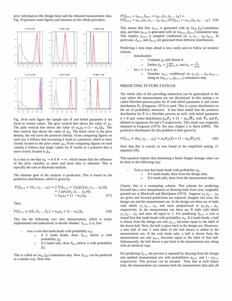
Fig. 10 presents some figures and intuition on the whole procedure.
Fig. 10:In each figure the sample size and belief parameter are
fixed to certain values. The grey vertical line shows the value of .
The pink vertical line shows the value of . The
blue vertical line shows the value of . The black curve is the prior
density; the red curve the posterior density. From comparing figures on
each row it follows that increasing leads to a posterior which is more
closely located to the prior center . From comparing figures on each
column it follows that larger values for results in a posterior that is
more closely located to .
It is easy to see that if , which means that the influence
of the prior vanishes as more and more data is obtained. This is
typically the case in Bayesian analysis.
The ultimate goal of the analysis is prediction. This is based on the
predictive distribution, which is given by:
(17)
Thus,
(18)
This has the following very nice interpretation, which is easily
implemented and understood: to decide whether , first
- toss a coin that lands heads with probability ;
o if it lands heads, draw below with
probability ;
o if it lands tails, draw below with probability
.
This is called an -simulation step. Now can be predicted
in a similar way. Note that:
(19)
This means that first is generated with an -simulation
step, and then is generated with an -simulation step.
This implies is sampled conditional on . In
particular, and are generated from different distributions.
Predicting time steps ahead is now easily seen to follow an iterative
scheme:
- Initialization
o Compute and choose
o Define
and
- for to do:
o Simulate conditional on
using an -simulation step.
PREDICTING FUTURE FATIGUE
The whole idea of the preceding subsection can be generalized to the
case where the measurements are not discretized. In this setting a so
called Dirichlet-process prior for with belief parameter and center
distribution (Ferguson, 1973) is used. This is a prior distribution on
the set of probability measures. It has been stated that the posterior
distribution for is a Dirichlet process as well, with belief parameter
and center distribution with and
defined in equations (6) and (7) respectively. This result was originally
obtained in Ferguson (1973). See also chapter 2 in Hjort (2009). The
predictive distribution for this problem is then given by
(20)
Note that this is exactly as was found in the simplified setting, cf.
equation (18).
This equation implies that simulating a future fatigue damage value can
be done in the following way:
- Toss a coin that lands heads with probability .
o If it lands heads, draw from the design data;
o If it lands tails, draw from the measurement data.
Clearly, this is a resampling scheme. This scheme for predicting
forward has a nice interpretation as drawing balls from urns, originally
pointed out in Blackwell and MacQueen (1973). Suppose
are given and forward predictions are required. Imagine two urns: the
design urn and the measurement urn. In the design urn there are balls
with labels and sizes proportional to
respectively. In the measurement urn there are balls with labels
and sizes all equal to . For predicting a coin is
tossed first that lands heads with probability . If it lands heads, a ball
is drawn from the design urn and becomes equal to the label of
the drawn ball. Next, the ball is place back in the design urn. Moreover,
a new ball of size with label of the ball drawn is added to the
measurement urn. If the coin lands tails, a ball is drawn from the
measurement urn and becomes equal to the label of that ball.
Subsequently, the ball drawn is put back in the measurement urn, along
with an identical copy.
For predicting the process is repeated by drawing from the design
and updated measurement urn with probabilities and
respectively. This process can be iterated. Note that at each future
time, the measurement urn contains both the measurement data plus all
predicted values. The representation using urns allows for a
straightforward implementation of the method.
User input
The only user input required is the specification of . As stated earlier,
specifies the amount of prior belief in the design data and can be
interpreted as the prior sample size. Fixing no matter how large
gives a truly Bayesian procedure in which the influence of the design
data vanishes as more and more data is obtained. If, for example, the
design data is to contain information comparable to years of
measurements, becomes , since the Monitas system
evaluates fatigue every six hours.
Comments on the proposed approach
Some advantages of the outlined approach are
- The resulting procedure does not make any parametric
assumptions, making it robust to model specification and
generally applicable.
- Prediction of future data follows from a simple urn scheme,
making the implementation fast and easy.
- Missing values in the measurement data can be handled in the
same way as missing future values.
The main simplifying assumption in the procedure is that the
are assumed to be exchangeable. This means that the
ordering in the data is neglected. A disadvantage of this assumption is
that short term predictions can be incorrect. Think of the situation
where at present large values of fatigue damage take place. Due to
clustering, it is to be expected to see large values in the next few days
as well. This is not incorporated in the present analysis. From an
application point of view this may not be harmful, since primary focus
of fatigue analyses are long-term predictions. Furthermore, one should
realize that the Monitas system only evaluates data once a month.
Monte Carlo simulation
The procedure above allows to predict fatigue accumulation to a
predefined future time. By repeating the procedure a different value for
the accumulated fatigue at this time will be obtained due to randomness
in the sampling mechanism. A number of realizations of fatigue
predictions are displayed in Fig. 11.
Fig. 11: Several simulated fatigue accumulations
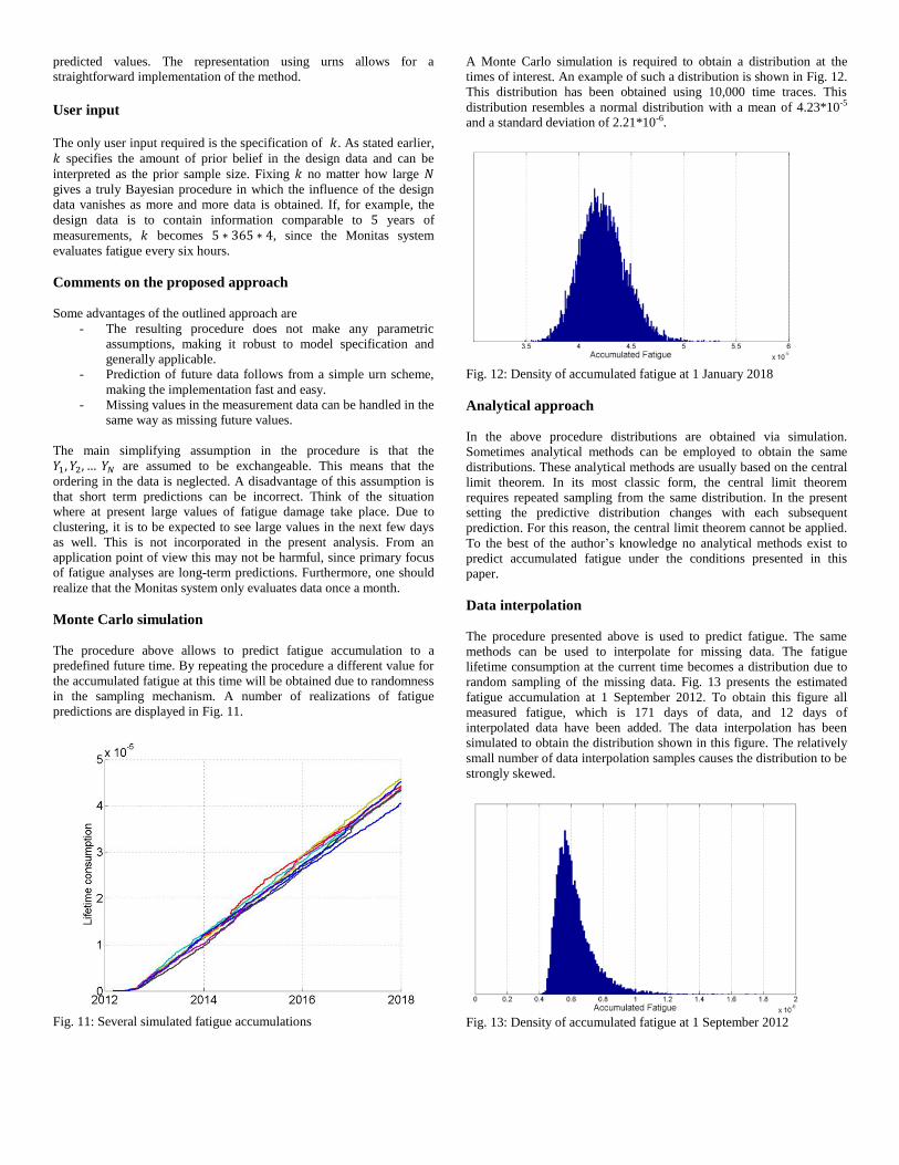
A Monte Carlo simulation is required to obtain a distribution at the
times of interest. An example of such a distribution is shown in Fig. 12.
This distribution has been obtained using 10,000 time traces. This
distribution resembles a normal distribution with a mean of 4.23*10-5
and a standard deviation of 2.21*10-6.
Fig. 12: Density of accumulated fatigue at 1 January 2018
Analytical approach
In the above procedure distributions are obtained via simulation.
Sometimes analytical methods can be employed to obtain the same
distributions. These analytical methods are usually based on the central
limit theorem. In its most classic form, the central limit theorem
requires repeated sampling from the same distribution. In the present
setting the predictive distribution changes with each subsequent
prediction. For this reason, the central limit theorem cannot be applied.
To the best of the author’s knowledge no analytical methods exist to
predict accumulated fatigue under the conditions presented in this
paper.
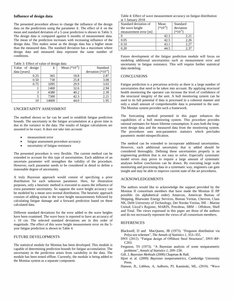
Data interpolation
The procedure presented above is used to predict fatigue. The same
methods can be used to interpolate for missing data. The fatigue
lifetime consumption at the current time becomes a distribution due to
random sampling of the missing data. Fig. 13 presents the estimated
fatigue accumulation at 1 September 2012. To obtain this figure all
measured fatigue, which is 171 days of data, and 12 days of
interpolated data have been added. The data interpolation has been
simulated to obtain the distribution shown in this figure. The relatively
small number of data interpolation samples causes the distribution to be
strongly skewed.
Fig. 13: Density of accumulated fatigue at 1 September 2012
Influence of design data
The presented procedure allows to change the influence of the design
data on the predictions using the parameter . The effect of on the
mean and standard deviation of a 5-year prediction is shown in Table 3.
The design data is compared against 6 months of measurement data.
The mean of the prediction increases with increasing influence of the
design data. This makes sense as the design data has a higher mean
than the measured data. The standard deviation has a maximum where
design data and measured data represent the same number of
conditions.
Table 3: Effect of value of design data
Value of design
data [years] Mean [*10-6] Standard
deviation [*10-6]
0.25 365 18.8 2.87
0.50 730 25.8 3.08
0.75 1095 29.9 3.03
1 1460 32.6 2.94
3 4380 40.2 2.39
5 7300 42.3 2.21
10 14600 44.0 1.95
UNCERTAINTY ASSESSMENT
The method shown so far can be used to establish fatigue prediction
bounds. The uncertainty in the fatigue accumulation at a given time is
due to the variance in the data. The results of fatigue calculations are
assumed to be exact. It does not take into account:
measurement error
fatigue assessment procedure accuracy
uncertainty of fatigue resistance
The presented procedure is very flexible. The current method can be
extended to account for this type of uncertainties. Each addition of an
uncertain parameter will strengthen the validity of the procedure.
However, each parameter needs to be considered in detail to define a
reasonable degree of uncertainty.
A truly Bayesian approach would consist of specifying a prior
distribution for each unknown parameter. Here, for illustration
purposes, only a heuristic method is executed to assess the influence of
extra parameter uncertainty. So suppose the wave height accuracy can
be modeled by a mean zero normal distribution. The heuristic approach
consists of adding noise to the wave height measurements followed by
calculating fatigue damage and a forward prediction based on these
calculated data.
Different standard deviations for the error added to the wave heights
have been examined. The wave buoy is reported to have an accuracy of
± 10 cm. The selected standard deviations are in this order of
magnitude. The effect of this wave height measurement error on the 5-
year fatigue prediction is shown in Table 4.
FUTURE DEVELOPMENTS
The statistical module for Monitas has been developed. This module is
capable of determining prediction bounds for fatigue accumulation. The
uncertainty in the prediction arises from variability in the data. The
module has been tested offline. Currently, the module is being added to
the Monitas system as a separate component.
Table 4: Effect of wave measurement accuracy on fatigue distribution
at 1 January 2018
Standard deviation of
the wave height
measurement error [m]
Mean
[*10-6] Standard
deviation
[*10-6] 0 42.3 2.21
0.05 42.5 2.26
0.10 43.1 2.27
0.20 44.5 2.37
Future development of the fatigue prediction module will focus on
modeling additional uncertainties such as measurement error and
uncertainty in fatigue resistance. This will require further statistical
data modeling.
CONCLUSIONS
Fatigue prediction is a precarious activity as there is a large number of
uncertainties that need to be taken into account. By applying structural
health monitoring the operator can increase the level of confidence of
the structural integrity of the unit. A hull monitoring system can be
used to its full potential if data is processed in a coherent manner and
only a small amount of comprehensible data is presented to the user.
The Monitas system provides such a framework.
The forecasting method presented in this paper enhances the
capabilities of a hull monitoring system. This procedure provides
rational estimates for future lifetime consumption. It uses both the long-
term design data and the measured data from the monitoring system.
The procedures uses non-parametric statistics which precludes
parametric model misspecification.
The method can be extended to incorporate additional uncertainties.
However, each additional uncertainty that is added should be
considered thoroughly. Defining these uncertainties properly is an
engineering problem that is not easy to solve. Especially systematic
model errors may prove to require a large amount of systematic
analyses before conclusions can be drawn. By executing large scale
monitoring and processing data in a systematic way, engineers can gain
insight and may be able to improve current state of the art procedures.
ACKNOWLEDGEMENTS
The authors would like to acknowledge the support provided by the
Monitas II consortium members that have made the Monitas II JIP
possible: (in alphabetical order) Amarcon, American Bureau of
Shipping, Bluewater Energy Services, Bureau Veritas, Chevron, Class
NK, Delft University of Technology, Det Norske Veritas, IHI – Marine
United, Lloyd’s Register, MARIN, Petrobras, SBM – Offshore, Shell
and Total. The views expressed in this paper are those of the authors
and do not necessarily represent the views of all consortium members.
REFERENCES
Blackwell, D and MacQueen, JB (1973). “Ferguson distribution via
Polya urn schemes”, The Annals of Statistics 1, 353--355.
DNV (2012). “Fatigue design of Offshore Steel Structures”, DNV-RP-
C203.
Ferguson, TS (1973). “A Bayesian analysis of some nonparametric
problems”, Annals of Statistics 1, 209--230.
Gill, J, Bayesian Methods (2008) Chapman & Hall.
Hjort et al. (2009) Bayesian nonparametrics, Cambridge University
Press.
Hanson, JL, Lübben, A, Aalberts, PJ, Kaminski, ML, (2010). “Wave
Measurements for the Monitas System,” Proc Offshore Technology
Conference, Houston, Texas, OTC 20869
L’Hostis, D, Kaminski, ML, Aalberts, PJ (2010). “Overview of the