My talk today is on the use of FBRM in the study of flocculation processes y y y p

M-2-146P

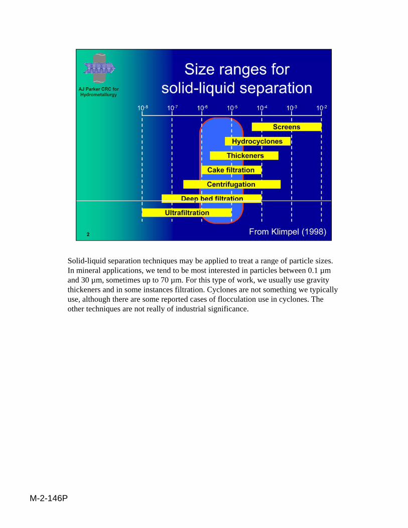
Solid-liquid separation techniques may be applied to treat a range of particle sizes. q p q y pp g pIn mineral applications, we tend to be most interested in particles between 0.1 µm and 30 µm, sometimes up to 70 µm. For this type of work, we usually use gravity thickeners and in some instances filtration. Cyclones are not something we typically use, although there are some reported cases of flocculation use in cyclones. The other techniques are not really of industrial significance.

M-2-146P

Gravity thickeners have a tank, which can have a diameter anywhere from about 5 y , ymeters up to 130 meters. The feed slurry comes in and, if it is a clarifier, is probably only 0.1 wt% solids. Most of the things we work with have somewhere between 2 and 30 wt% solids coming in. Typically, a flocculant is added. There is a feedwell where there is mixing and turbulence. The solids are flocculated and come out in the settling zone. The liquor flows off and can either be recycled or goes on to further processing.

We get compaction through the formation of a bed and often there is extensive raking to try to express more liquor out of the aggregates that form. Ultimately, there is an underflow that can be 70 wt% solids depending on the initial particle size. In the Bayer process for the treatment of bauxite there is 50 wt% underflow solids and it develops such that it can be virtually pumped out as a paste and then d di ddry-disposed.

M-2-146P

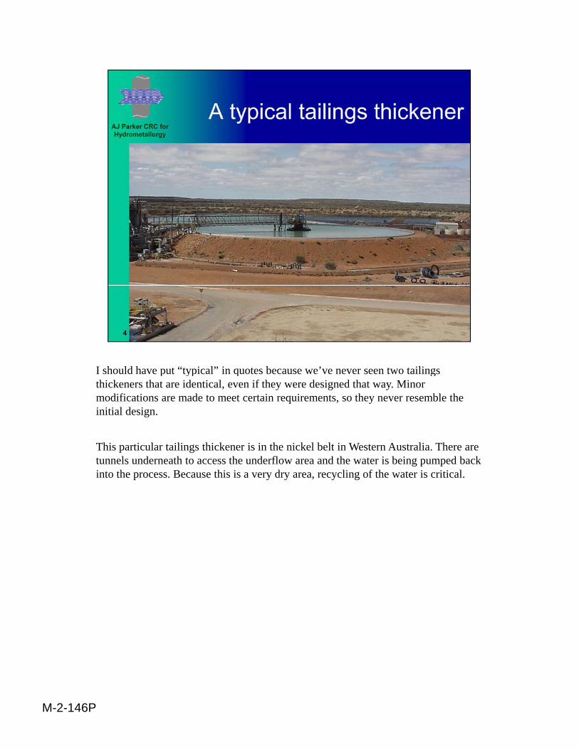
I should have put “typical” in quotes because we’ve never seen two tailings p yp q gthickeners that are identical, even if they were designed that way. Minor modifications are made to meet certain requirements, so they never resemble the initial design.

This particular tailings thickener is in the nickel belt in Western Australia. There are tunnels underneath to access the underflow area and the water is being pumped back g p pinto the process. Because this is a very dry area, recycling of the water is critical.

M-2-146P

In studying a thickener, we know our effective settling area and our volumetric flow y g , grate in, so we can calculate a normal rise velocity for our thickener – the rate at which the liquor is coming up.

To get effective operation in a thickener, we need to have our particles settling at a certain rate that must be in excess of the rise velocity. We work on about twice the rise velocity as a minimum value, but different people will work at different y , p pmultipliers.

M-2-146P

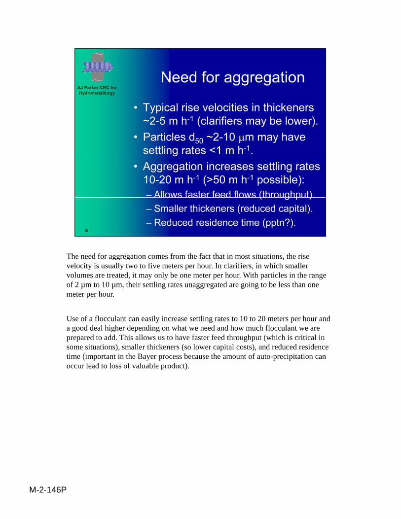
The need for aggregation comes from the fact that in most situations, the rise gg g ,velocity is usually two to five meters per hour. In clarifiers, in which smaller volumes are treated, it may only be one meter per hour. With particles in the range of 2 µm to 10 µm, their settling rates unaggregated are going to be less than one meter per hour.

Use of a flocculant can easily increase settling rates to 10 to 20 meters per hour and y g pa good deal higher depending on what we need and how much flocculant we are prepared to add. This allows us to have faster feed throughput (which is critical in some situations), smaller thickeners (so lower capital costs), and reduced residence time (important in the Bayer process because the amount of auto-precipitation can occur lead to loss of valuable product).

M-2-146P

Please excuse the sweeping generalizations in this overhead, which is only intended p g g , yto highlight the differences between the two processes. In crystallization, mass typically increases. In flocculation, mass stays constant and it is the effective volume that increases. In crystallization, particle number rises (though in the case of agglomeration, it goes down). In flocculation, the effective number decreases dramatically. Particle density may be a constant in crystallization, but in flocculation we get very low aggregate densities.

Size changes can be quite large in crystallization, but in flocculation we can take a 5µm particle and turn it into a 3mm aggregate within a matter of seconds. Size change being irreversible in crystallization isn’t necessarily true, as attrition is possible. However, in flocculation, the aggregates are very fragile. The low density of aggregates that form and the fact that we have very fragile species are probably th t iti l i t t b b t fl l tithe two critical points to remember about flocculation.

M-2-146P

Flocculation is achieved by bridging of particles by high molecular weight y g g p y g gpolymers. The flocculants themselves can be polymers in the range of molecular weight 10 to 20 million. In solution they will have radii in the order of 130 to 200 nm. If you extended them out in a straight chain, they would be about 20 µm. There are a number of chains that bridge between the particles forming a very loose aggregate, so it’s no surprise that these are quite fragile.

M-2-146P

For typical flocculants, in most mineral applications a fair degree of anionic charge yp , pp g gis introduced. On the other hand are cationic materials, which are not usually used in the minerals industry. They are more common in water treatment.

M-2-146P

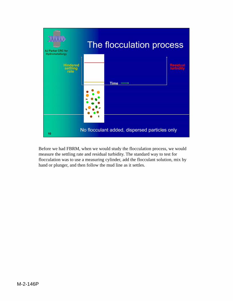
Before we had FBRM, when we would study the flocculation process, we would , y p ,measure the settling rate and residual turbidity. The standard way to test for flocculation was to use a measuring cylinder, add the flocculant solution, mix by hand or plunger, and then follow the mud line as it settles.

M-2-146P

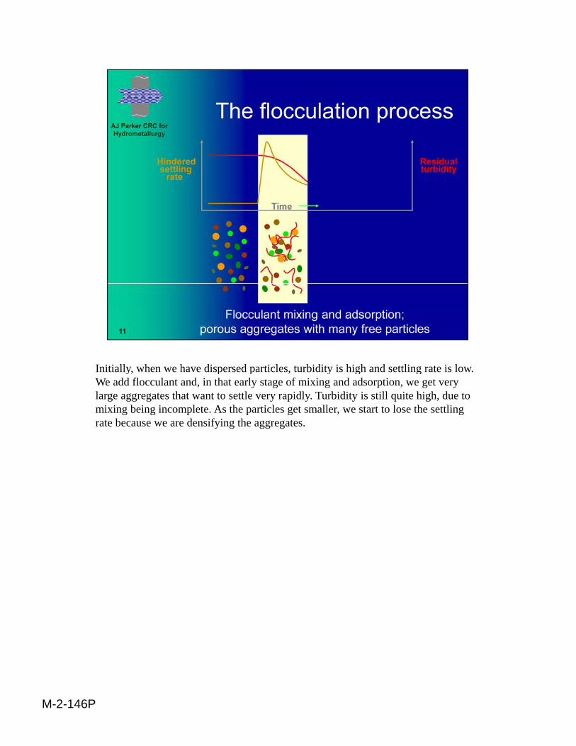
Initially, when we have dispersed particles, turbidity is high and settling rate is low. y, p p , y g gWe add flocculant and, in that early stage of mixing and adsorption, we get very large aggregates that want to settle very rapidly. Turbidity is still quite high, due to mixing being incomplete. As the particles get smaller, we start to lose the settling rate because we are densifying the aggregates.

M-2-146P

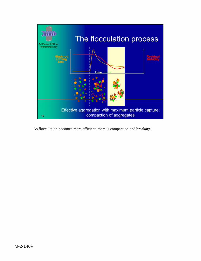
As flocculation becomes more efficient, there is compaction and breakage. , p g

M-2-146P

As we continue to mix, we shear the aggregates, they become smaller fragments, , gg g , y g ,turbidity goes back up, and settling rate drops back down again. It is a dynamic process in which there is considerable overlap between all of these processes.

M-2-146P

While there has been a massive amount of flocculation work done in the literature, ,most of that work was on colloidal materials or polystyrene latexes using low molecular-weight polymers, and therefore of minimal relevance to real systems. In industry, there has not been a great degree of science. The understanding of thickening is quite unsophisticated in comparison to crystallization. We see ourselves as a bridge between the two groups, trying to bring together knowledge that has been developed at a fundamental level and make use of it in industrial sit ationssituations.

M-2-146P

We’re based in Perth, in Western Australia. There are other people in our group who , p p g pwork in Melbourne. We take FBRM probes on site to mineral-processing operations to do measurements. The red dots represent areas where our probes are being used. Some of these are related to our generic program on a large project sponsored by a number of companies. Others are to solve specific company problems.

We’ve been using FBRM probes since 1995. Most of this work has been in industry-g p ysponsored projects. We currently have 27 sponsors of a project devoted to the study of thickeners. I have primary responsibility for use of the FBRM probes, and as a chemist, my interest is in trying to interpret what is happening in the processes we study.

M-2-146P

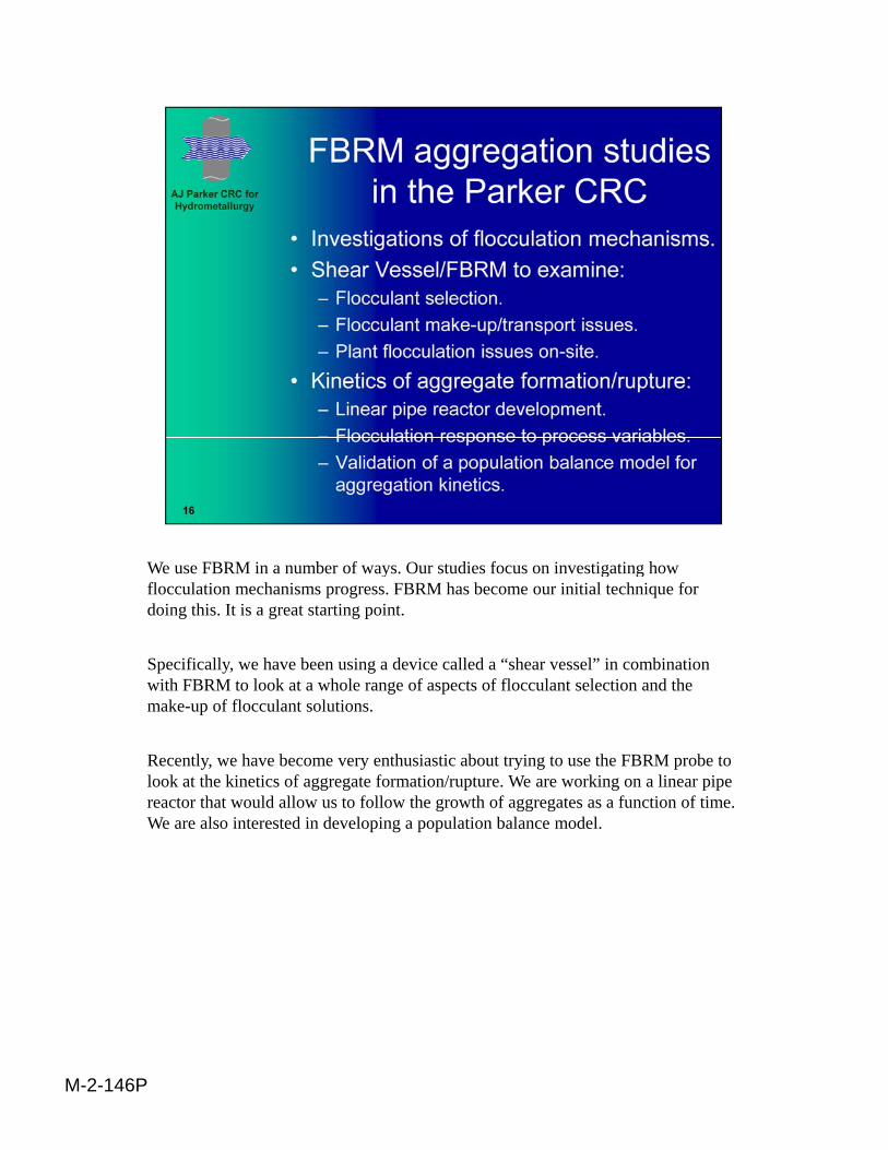
We use FBRM in a number of ways. Our studies focus on investigating how y g gflocculation mechanisms progress. FBRM has become our initial technique for doing this. It is a great starting point.

Specifically, we have been using a device called a “shear vessel” in combination with FBRM to look at a whole range of aspects of flocculant selection and the make-up of flocculant solutions. p

Recently, we have become very enthusiastic about trying to use the FBRM probe to look at the kinetics of aggregate formation/rupture. We are working on a linear pipe reactor that would allow us to follow the growth of aggregates as a function of time. We are also interested in developing a population balance model.

M-2-146P

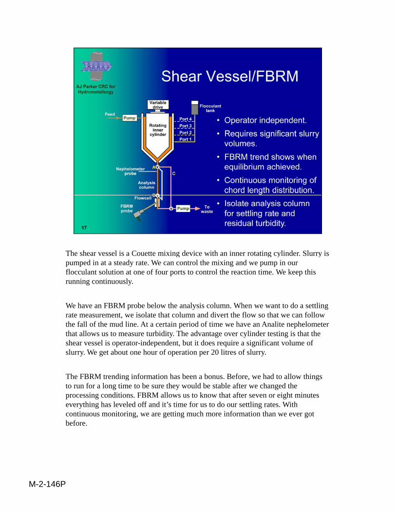
The shear vessel is a Couette mixing device with an inner rotating cylinder. Slurry is g g y ypumped in at a steady rate. We can control the mixing and we pump in our flocculant solution at one of four ports to control the reaction time. We keep this running continuously.

We have an FBRM probe below the analysis column. When we want to do a settling rate measurement, we isolate that column and divert the flow so that we can follow ,the fall of the mud line. At a certain period of time we have an Analite nephelometer that allows us to measure turbidity. The advantage over cylinder testing is that the shear vessel is operator-independent, but it does require a significant volume of slurry. We get about one hour of operation per 20 litres of slurry.

The FBRM trending information has been a bonus. Before, we had to allow thingsThe FBRM trending information has been a bonus. Before, we had to allow things to run for a long time to be sure they would be stable after we changed the processing conditions. FBRM allows us to know that after seven or eight minutes everything has leveled off and it’s time for us to do our settling rates. With continuous monitoring, we are getting much more information than we ever got before.

M-2-146P

This was our early shear vessel. It was not designed for FBRM probes, as we y g p ,couldn’t put the probe into it at an angle, so in 1995 we added a little cell that diverted the flow to allow us to get reasonable presentation to the probe. This worked very well in most systems, though there were some rapidly settling systems with which we had problems.

This vessel is actually quite transportable. Without the FBRM probe, it has been to y q p p ,about 15 different sites across Australia.

M-2-146P

The vessel we use now has been scaled down considerably, making it much easier to y, gtransport. We have a much better flow cell arrangement for the FBRM probe.

On the left is our lab version. On the right the acrylic outer has been replaced with a jacketed stainless-steel version for high-temperature Bayer process studies. We recently sent a probe and shear vessel to Ireland for work there in an aluminum refinery. y

M-2-146P

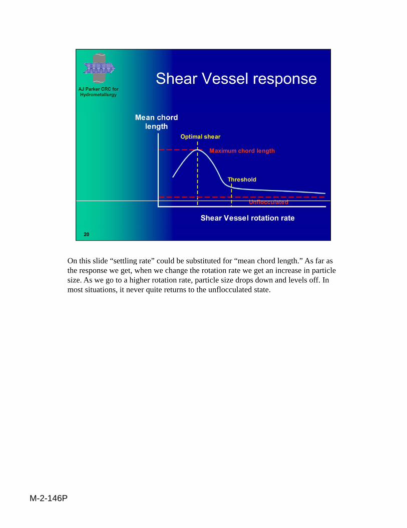
On this slide “settling rate” could be substituted for “mean chord length.” As far as g gthe response we get, when we change the rotation rate we get an increase in particle size. As we go to a higher rotation rate, particle size drops down and levels off. In most situations, it never quite returns to the unflocculated state.

M-2-146P

With time, we’ve become very good at interpreting what we are seeing. If we , y g p g gflocculate well, the unweighted counts drop down to a very low level and the square-weighted distribution shifts across quite substantially.

If we’re not flocculating well (i.e., if we’re forming aggregates and leaving particles behind), we get bi-modal distributions. Notice the square-weighted distribution shows no effect of that at all. The square-weighted numbers give us the best q g gcorrelation to settling rate.

M-2-146P

In a situation where we are adding flocculant and we see the mean chord length go g g gup with the mean square-weighted chord length also going up, we know we have good, efficient flocculation. If the mean chord length does not change but the mean square-weighted chord length goes up, that is a situation where we are getting large aggregates, but poor fines capture.

In situations where the mean chords increase but the mean square-weighted chord q glength does not increase, that implies we are getting a mechanism that predominantly goes through fines capture. The small particles are aggregating prior to large particles being incorporated. None of the aggregates formed are larger than the largest particles there initially. We have some situations where it will start off like this, but once all of the fines are consumed, it will start going up under normal circumstances. Finally, there is the situation where we have added too much fl l t W t t i t h thi k h ti fl l ti b tflocculant. We get to a point where we think we have optimum flocculation, but when we add more flocculant, we get dispersion. In practice, this is rarely observed.

M-2-146P

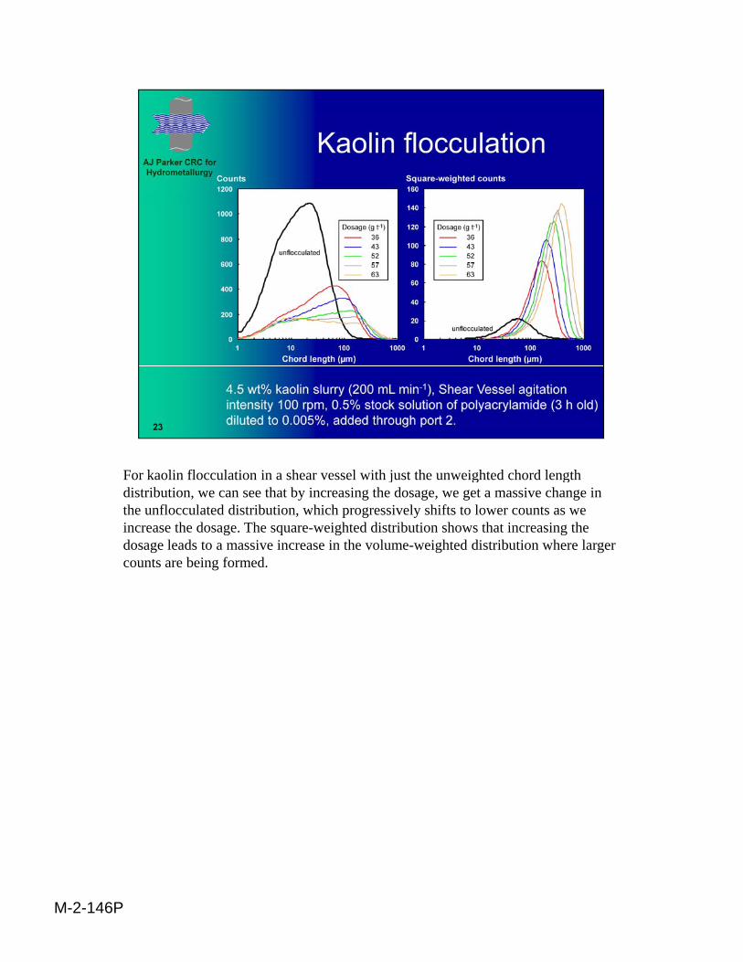
For kaolin flocculation in a shear vessel with just the unweighted chord length j g gdistribution, we can see that by increasing the dosage, we get a massive change in the unflocculated distribution, which progressively shifts to lower counts as we increase the dosage. The square-weighted distribution shows that increasing the dosage leads to a massive increase in the volume-weighted distribution where larger counts are being formed.

M-2-146P

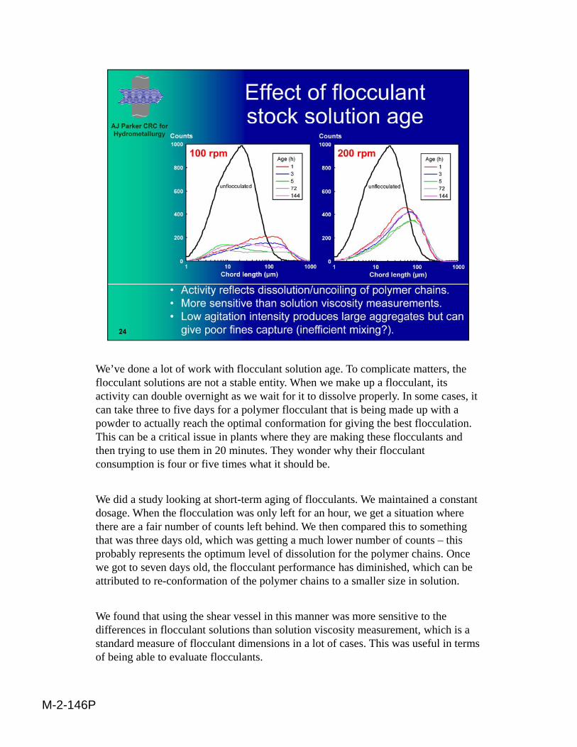
We’ve done a lot of work with flocculant solution age. To complicate matters, the g p ,flocculant solutions are not a stable entity. When we make up a flocculant, its activity can double overnight as we wait for it to dissolve properly. In some cases, it can take three to five days for a polymer flocculant that is being made up with a powder to actually reach the optimal conformation for giving the best flocculation. This can be a critical issue in plants where they are making these flocculants and then trying to use them in 20 minutes. They wonder why their flocculant cons mption is fo r or fi e times hat it sho ld beconsumption is four or five times what it should be.

We did a study looking at short-term aging of flocculants. We maintained a constant dosage. When the flocculation was only left for an hour, we get a situation where there are a fair number of counts left behind. We then compared this to something that was three days old, which was getting a much lower number of counts – this

b bl t th ti l l f di l ti f th l h i Oprobably represents the optimum level of dissolution for the polymer chains. Once we got to seven days old, the flocculant performance has diminished, which can be attributed to re-conformation of the polymer chains to a smaller size in solution.

We found that using the shear vessel in this manner was more sensitive to the differences in flocculant solutions than solution viscosity measurement, which is a t d d f fl l t di i i l t f Thi f l i t

M-2-146P

standard measure of flocculant dimensions in a lot of cases. This was useful in terms of being able to evaluate flocculants.

Aggregate density can change greatly depending on the amount of agitation that is gg g y g g y p g gapplied to it. This slide shows a typical response. Mild mixing favors the open structures. Generally, when increased shear is applied, the aggregates will either rupture or densify themselves.

M-2-146P

In 1999 we took settling rate data acquired over a range of conditions and tried to g q gcorrelate it to the mean square-weighted chord length. We got what we thought at the time was a decent relationship, but we had neglected to isolate the effects of mixing.

The actual aggregate density had a big effect on what we were seeing. When we repeated the experiments at a fixed RPM over a range of dosages, we were able to p p g g ,get a nice correlation between settling rate and mean square-weighted chord length. When we did the same experiment at a different RPM, we saw a different relationship. This was clear evidence of the change in aggregate density. To get a settling rate of ten meters per hour, we had to have a much larger aggregate as measured by FBRM.

M-2-146P

We’ve done off-line measurements of aggregate densities using a device we made gg g gmore than ten years ago called a “floc density analyzer.” Effectively, this is a video camera system in a very dilute flow cell where we monitor settling rates of individual aggregates and measure their size.

We were able to show that aggregates formed at 100 RPM and separated at three or four meters per hour had a volume ratio of liquor to solids of about 60:1. This is p qcompared to aggregates formed at 200 RPM, where the liquor to solids was about 40:1. That is quite a large change in density.

The shear vessel/FBRM combination gave us a good qualitative way of comparing our density. We will never actually be able to extract density numbers from this relationship, but we can go to a site and talk about changes to aggregate densityrelationship, but we can go to a site and talk about changes to aggregate density depending on the flocculant system being used, without having to go through a very long and involved process of actually doing floc density measurements.

M-2-146P

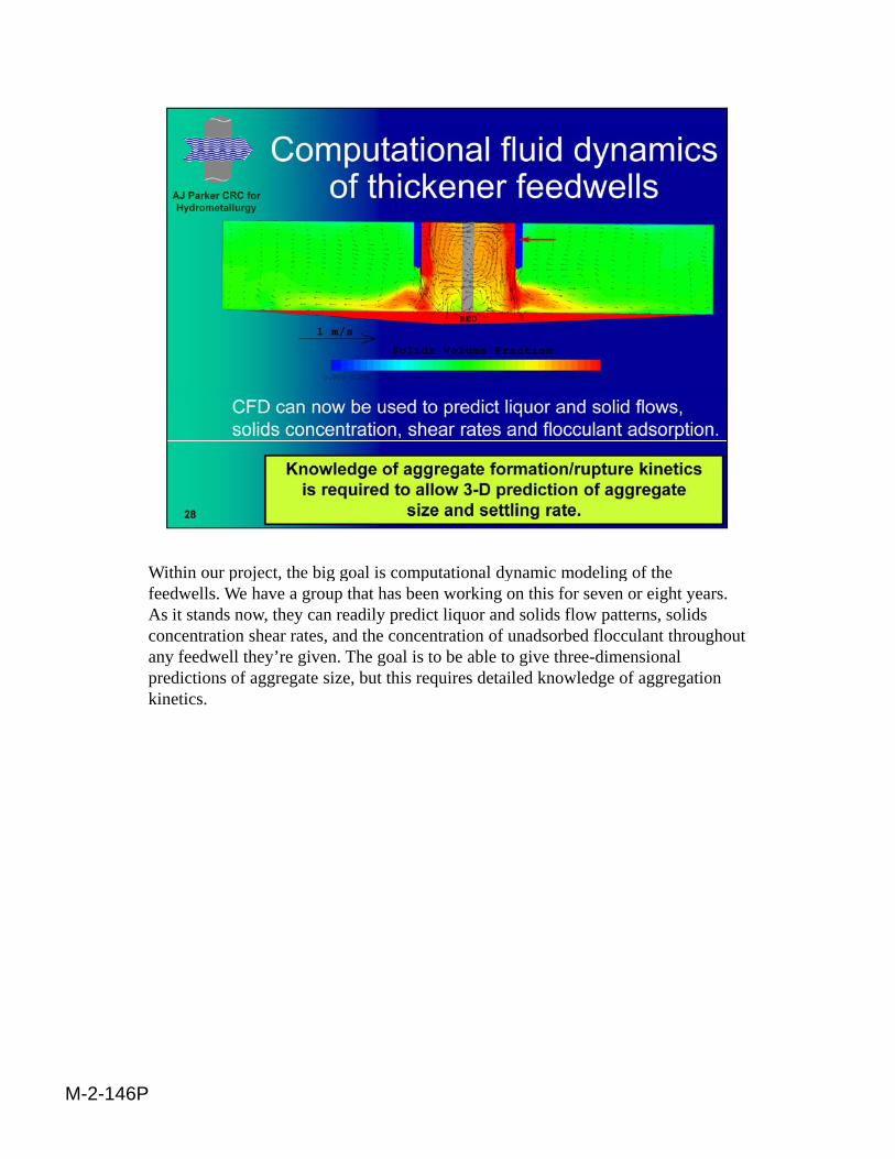
Within our project, the big goal is computational dynamic modeling of the p j , g g p y gfeedwells. We have a group that has been working on this for seven or eight years. As it stands now, they can readily predict liquor and solids flow patterns, solids concentration shear rates, and the concentration of unadsorbed flocculant throughout any feedwell they’re given. The goal is to be able to give three-dimensional predictions of aggregate size, but this requires detailed knowledge of aggregation kinetics.

M-2-146P

Many people have tried to study flocculation kinetics, but the majority of these y p p y , j ystudies have been in stirred tanks under batch conditions, with the shear rate poorly controlled and excessive residence times.

The other problem has been the lack of suitable techniques to characterize the size of aggregates formed. John Gregory proposed a device based on turbidity fluctuations. It works well in dilute slurries, but isn’t suitable for us. The FBRM ,probes effectively opened up this area of study for us. The other critical step was the use of a linear pipe reactor to give tight control over shear and reaction time.

M-2-146P

Our use of a pipe reactor was pretty much inspired by the work of Richard Williams p p p y p yin the early 1990s. He flocculated silica particles in a stirred tank and then used FBRM to follow aggregate rupture as the particles flowed through a pipe of known length and diameter.

M-2-146P

By changing the flow rate, Williams was able to study the effect of increasing shear y g g , y grate on the aggregate size, which steadily decreased. What we’ve done differently also is to flocculate within a pipe.

M-2-146P

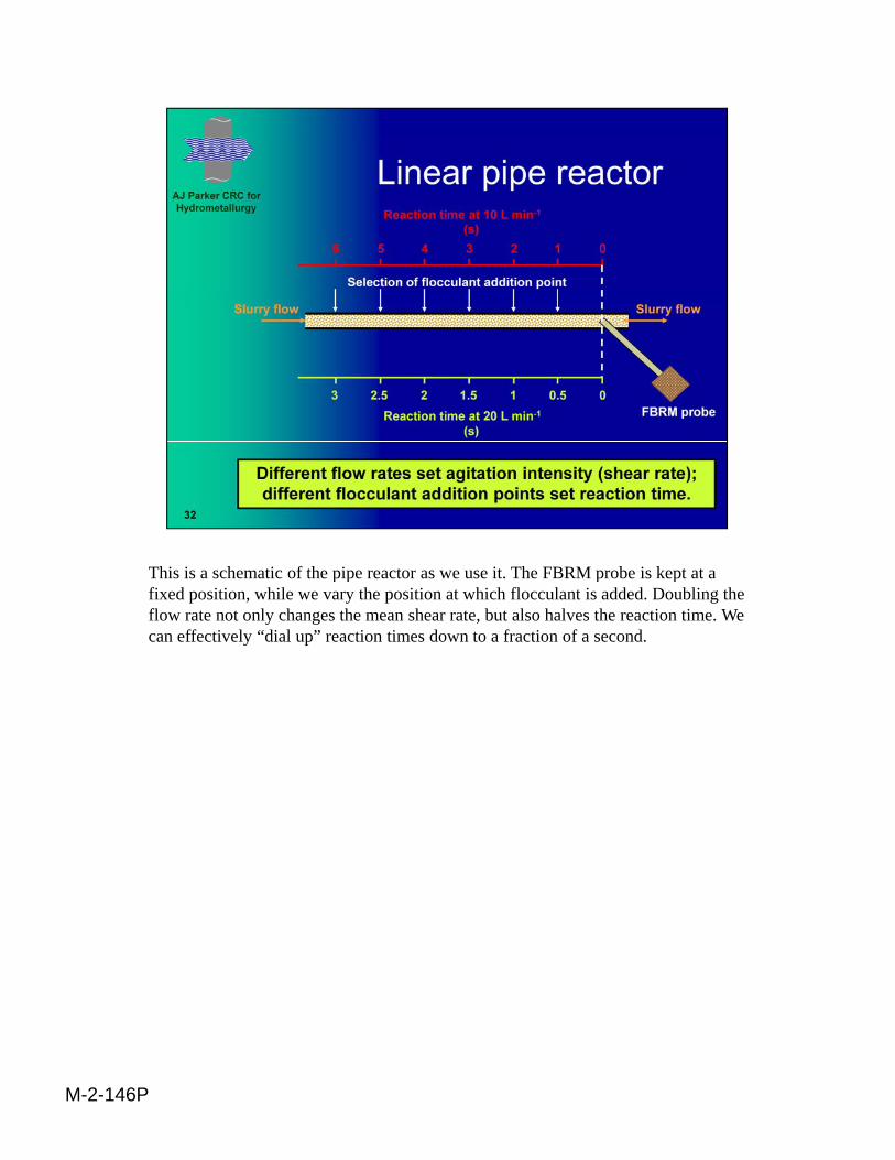
This is a schematic of the pipe reactor as we use it. The FBRM probe is kept at a p p p pfixed position, while we vary the position at which flocculant is added. Doubling the flow rate not only changes the mean shear rate, but also halves the reaction time. We can effectively “dial up” reaction times down to a fraction of a second.

M-2-146P

The image here shows our very first attempt at using a pipe reactor, which was g y p g p p ,underneath a mineral sands tailings thickener south of Perth. On-site measurements are often necessary due to the large volumes of slurry required. Ideally we seek feed slurries at high solids concentrations so we can then dilute across a range of concentrations. We can add lengths of pipe to the system to give us longer reaction times. Flow rates are typically 10 to 30 litres per minute, although we have gone outside that range depending on the pipe diameter.

M-2-146P

The image on the left shows a pipe reactor set up by PhD student Alex Heath to g p p p yobtain data on calcite flocculation to validate the population balance model he was developing. Along the length of the pipe you can see outlet tubes that connected to a manometer, allowing him to get pressure drop measurements and thereby confirm predicted shear rates. There was also a settling column almost immediately after the FBRM probe.

The image on the right shows a pipe reactor in use at a Bayer processing operation, using slurries at 100ºC and in strong caustic liquors. Our procedures had to be modified to ensure safe operation with such dangerous slurries.

M-2-146P

You’ve already heard a number of others mention population balance modeling, so I y p p g,won’t go into any great detail. Hounslow developed equations to describe aggregation, predicting the change in particle concentrations in a series of discretized size channels. However, Hounslow was dealing with crystallization, with rupture not being considered. Patrick Spicer later modified Hounslow’s equations to include aggregate rupture. The challenges that Alex Heath has faced in his population balance development were to incorporate flocculant mixing and the effects of irre ersible r pt re and aggregate porositeffects of irreversible rupture and aggregate porosity.

M-2-146P

The possible size response as a function of reaction time is shown here p pschematically and certainly not to scale. The initial induction period reflects the time required to mix the flocculant throughout the slurry, and this will depend upon viscosity and the applied shear. The size then increases up to a maximum value, which is determined by both the shear rate and the flocculant dosage. At this maximum, aggregate breakage has become a significant factor.

The Spicer population balance is really a coagulation model, with reversible rupture giving a plateau in the size at longer times. However, for most hydrometallurgical systems, irreversible rupture means there is a peak in aggregate size, with longer reaction times leading to a much smaller sizes.

M-2-146P

Here we see unweighted chord length distributions for two different reaction times. g gFor the slurry of 9.4 grams per litre, it appears that aggregation has almost progressed to its highest level after six seconds. In contrast, at 27.5 grams per litre, much longer times are required to achieve good fines capture. This clearly demonstrates the inefficient mixing that takes place at higher solids, which needs to be included in any population balance model.

M-2-146P

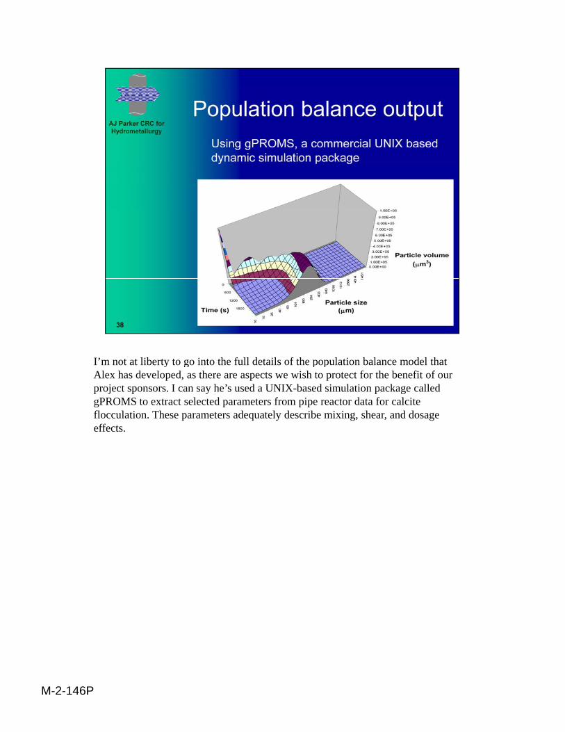
I’m not at liberty to go into the full details of the population balance model that y g p pAlex has developed, as there are aspects we wish to protect for the benefit of our project sponsors. I can say he’s used a UNIX-based simulation package called gPROMS to extract selected parameters from pipe reactor data for calcite flocculation. These parameters adequately describe mixing, shear, and dosage effects.

M-2-146P

The experimental data seen here for different shear rates shows that the model fits pwell. The dashed line for the lowest shear rate suggests this data needs to be viewed with caution, as some settling was observed within the pipe. The good fit is perhaps not a surprise, as this data was used in parameter estimation. However, we also conducted a number of separate tests in which two variables were changed simultaneously. The model worked well in predicting these results.

A major consideration with any population balance modeling is how chord length data is used to give size information that the population balance requires. It is important to note that we’ve not tried to predict size distributions from the pipe reactor data, but are simply dealing with a mean aggregate size. We are confident that the mean square-weighted chord length represents an acceptable estimate of this.

M-2-146P

We’ve also used a PVM probe to examine material flocculated in the pipe reactor. p p pThe images shown here are for a 2% kaolin slurry. The unflocculated slurry shows minimal evidence of aggregation, although there is always some residual degree of coagulation with kaolin. When we add 8 grams per ton of flocculant to it, we begin to see formation of moderately distinct aggregates. They are not particularly large. When we get to about 15 grams per ton, the fines pretty much disappear from the slurry. This is a reaction time of about three seconds, so it doesn’t take much for these things to formthese things to form.

M-2-146P

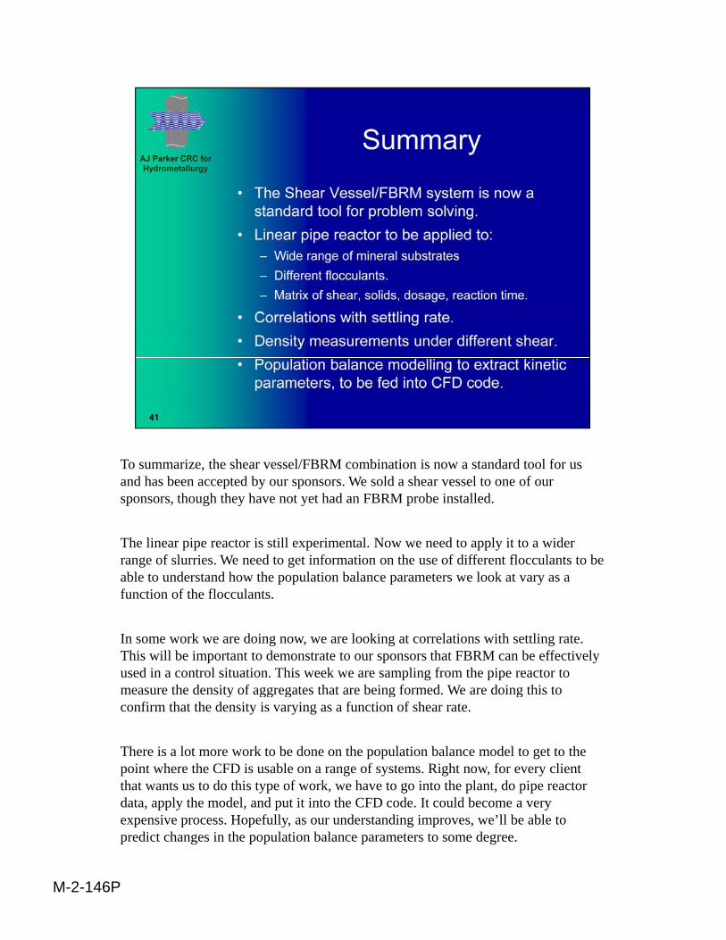
To summarize, the shear vessel/FBRM combination is now a standard tool for us ,and has been accepted by our sponsors. We sold a shear vessel to one of our sponsors, though they have not yet had an FBRM probe installed.

The linear pipe reactor is still experimental. Now we need to apply it to a wider range of slurries. We need to get information on the use of different flocculants to be able to understand how the population balance parameters we look at vary as a p p p yfunction of the flocculants.

In some work we are doing now, we are looking at correlations with settling rate. This will be important to demonstrate to our sponsors that FBRM can be effectively used in a control situation. This week we are sampling from the pipe reactor to measure the density of aggregates that are being formed. We are doing this tomeasure the density of aggregates that are being formed. We are doing this to confirm that the density is varying as a function of shear rate.

There is a lot more work to be done on the population balance model to get to the point where the CFD is usable on a range of systems. Right now, for every client that wants us to do this type of work, we have to go into the plant, do pipe reactor data, apply the model, and put it into the CFD code. It could become a very

M-2-146P

data, apply the model, and put it into the CFD code. It could become a very expensive process. Hopefully, as our understanding improves, we’ll be able to predict changes in the population balance parameters to some degree.

Q: What’s the mechanism for the flocculants adsorbing on your particles?Q g y p

PF: Under most solution conditions for oxide minerals you have a negatively charged surface, but as long as you are not too far away from the isoelectric point, you still have a fraction of non-charged sites on the particle surface. Adsorption is predominantly through hydrogen bonding of the nonionic amide groups onto these neutral groups. Any hydrolysis of the flocculant just gives a g p g p y y y j ghigher chance of bridging through greater chain extension. That’s why the anionic flocculants are more widely used. The non-ionic ones tend to coil up and require higher dosages.

M-2-146P