In Partial Fulfillment of the Requirements For the Degree of
MASTER OF SCIENCE
In the Graduate College
THE UNIVERSITY OF ARIZONA
1 9 7 6
STATEMENT BY AUTHOR
This thesis has been submitted in partial fulfillment of requirements for an advanced degree at The University of Arizona and is deposited in the University Library to be made available to borrowers under rules of the Library.
Brief quotations from this thesis are allowable without special permission, provided that accurate acknowledgment of source is made. Requests for permission for extended quotation from or reproduction of this manuscript in whole or in part may be granted by the head of the major department or the Dean of the Graduate College when in his judgment the proposed use of the material is in the interests of scholarship. In all other instances, however, permission must be obtained from the author.
SIGNED: QlujjJljLO t)
APPROVAL BY THESIS DIRECTOR
This thesis has been approved on the date shown below:
fessor ofAssociateAgricultural Economics
Date ^ / *
ACKNOWLEDGMENTS
I wish to acknowledge the efforts of my major professor, John C.
Day, whose very careful reviews and meticulous comments contributed much
to the completeness of this thesis. I also thank Dr. Reuben N. Weisz,
who started me on this effort and Dr. Dennis L. Larson, who provided
both moral and financial support to me. Those serving on my orals
committee were Dr. Roger W. Fox and Dr. Robert C. Angus. Drs. Day, Fox
and Angus are members of the Department of Agricultural Economics and
Dr. Larson of the Department of Soils, Water and Engineering at The
University of Arizona. Dr. Weisz is with the Economic Research Service,
U. S. Department of Agriculture.
In constructing the representative farm of Chapter II, I was
assisted immeasurably by the expertise and experience of Dr. Scott
Hathorn, Jr. and Mr. Charles Robertson of The University of Arizona Farm
Management Office. Others contributing to this effort were Dr. C. Curtis
Cable, Dr. Robert S. Firch and N. Gene Wright of the Department of Agri
cultural Economics and Allen D. Halderman, Agricultural Engineering
Specialist, all of The University of Arizona. Many unattributed facts
and opinions about Pinal County and Arizona farming and irrigation are
from informal discussions with these gentlemen during the spring and
summer of 1976.
I would also like to thank Carol J. Schwager and Ginger L.
Garrison for decrypting and typing my several drafts and Paula Tripp
for her very professional job in typing the final copy of this thesis.
iii
iv
Finally, I would like to acknowledge the many contributions of Charles D.
Sands II a fellow researcher at The University of Arizona trying to shed
some sunlight on solar-electric power.
I dedicate this thesis to the memory of my mother, Jeanne B.
Towle, who passed on during its preparation.
TABLE OF CONTENTS
Page
LIST OF TABLES...................................................... vii
LIST OF ILLUSTRATIONS................................... ix
ABSTRACT........................... ................................. x
CHAPTER
I INTRODUCTION AND BACKGROUND ............................... 1
Arizona Agriculture — Water and Energy .............. 1Groundwater U s e ................................... 4Energy U s e ......................................... 4
Statement of Problem ................................... 7Objective.............................................. 8Procedure .............................................. 9
Pinal County Background ........................... 9Conventional Energy Sources Used in Pumping . . . . 10Analysis.......... 12
II DESCRIPTION AND BUDGETING OF THE REPRESENTATIVE FARM . . . . 17
Farm S i z e ................................................ 17Representative Crop M i x ..................................18Solar Farm Irrigation System...................... . . . 22Economic Environment for Solar Farm .................. 32
Prices................................................ 32Solar Farm B u d g e t ....................................34R e t u r n s .............................................. 42
III DETERMINATION OF ECONOMICALLY JUSTIFIABLE INITIALCOST OF SOLAR SYSTEM........................................45
Computational Approach ................................. 45Justifiable Investment in Solar System ................. 47
Justifiable Solar System Initial Cost ................. 53
v
TABLE OF CONTENTS— Continued
Page
Justifiable Cost before O&M Charges .............. 55Justifiable Cost after O&M Charges .............. 59Other Factors Affecting Justifiable Cost ........... 60
IV DESCRIPTION AND ASSESSMENT OF BASIC SOLAR SYSTEMAND ALTERNATIVES......................................... 62
Basic Solar System P l a n t ............................. 62Physical Description......................... .. . 64Estimate of Basic Solar Plant Cost ............... 66
Solar Energy " P r i c e " ................................. 68Further Considerations ............................... 73
Options for Matching Basic Solar System toFarm Irrigation Schedule ....................... 74
Direct Steam-driven Well Power Systems .......... 78Water Conservation Alternatives ................... 79Effect of Increasing Pumping Lifts on Costs . . . . 80Effect of Overall Pumping Efficiency ............ 82Effect of Rising Energy Price on Farm
Financial Position ............................. 83Conclusion............................................ 87
V DISCUSSION OF RESULTS AND CONCLUSIONS ........................ 88
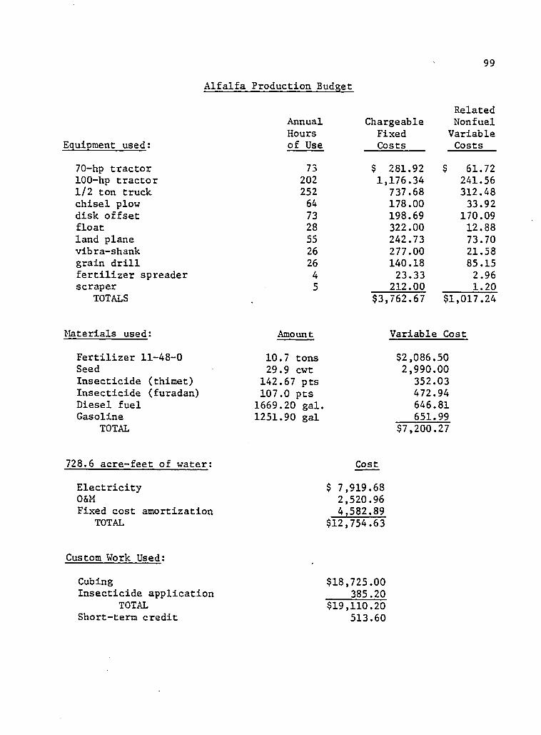
APPENDIX: PRODUCTION BUDGETS FOR SOLAR F A R M ................... 94
LIST OF REFERENCES................................................... 101
vi
LIST OF TABLES
Table Page
1. Comparison of U. S. and Arizona Crop Production.......... 2
2. Energy Used in Pumping Groundwater in Arizona ............ 6
3. Pinal County Cropping Pattern, Field Crops .............. 20
4. Solar Farm Crop Water Application Pattern — WaterUsed per Acre in Acre-inches........................... 24
5. Solar Farm Crop Water Application Pattern — TotalWater Used in Acre-feet....................................26
6. Revised Irrigation Schedule for Wheat ..................... 29
7. Solar Farm Implicit Irrigation Efficiencies . . .......... 29
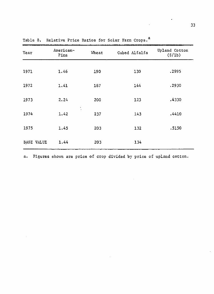
8. Relative Price Ratios for Solar Farm Crops .............. 33
9. Operating Schedule for Solar Farm Wells ................... 35
10. Cost of Pumping Water in 1976, Well No. 1 ....................37
11. Cost of Pumping Water in 1976, Well No. 2 ....................38
12. Cost of Pumping Water in 1976, Well No. 3 .................... 39
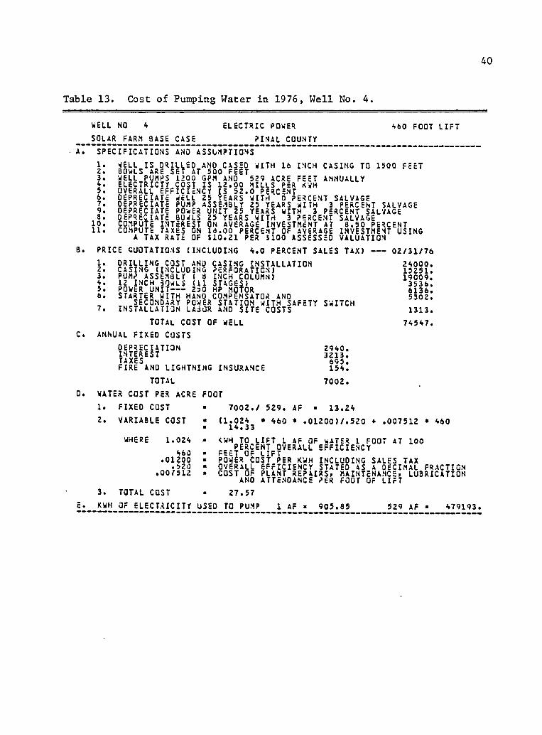
13. Cost of Pumping Water in 1976, Well No. 4 ....................40
14. Solar Farm Costs and Returns S u m m a r y ....................... 44
15. Annual Costs of Electricity to Solar F a r m ................... 51
16. Justified Investment in Solar Equipment for VariousValues of Pumping Lift, Pumping Efficiency, andDiscount Rates (1976 dollars) ........................... 54
17. Justified Initial Costs for Collector Section,Generator Section, and Total Solar Power Plantfor Solar Farm Financial Breakeven in Thousandsof 1976 Dollars .......................................... 58
19. Matching of Irrigation Needs with Sunlight Available . . . 75
20. Effect of Rising Energy Prices on Solar Farm NetR e t u r n s ................................................ 86
/
LIST OF ILLUSTRATIONS
Figure Page
1. Total Cost (Fixed Plus Variable) of Pumping OneAcre-foot of Water by Source of Energy for SelectedPumping Lifts, Eloy Area, Pinal County, 1976(from Hathorn, 1976) .................................... 11
2. Pinal County Cropping Pattern Trends ..................... 21
3. Basic Arrangement of Components for Solar System ........ 63
ix
ABSTRACT
Arizona agriculture is a major consumer of energy. The use of
solar power to pump groundwater would free Arizona farmers from reliance
on uncertain energy supplies. Using a representative farm model, the
economically feasible upper limit for initial investment in solar equip
ment is derived for alternative pumping situations on a Pinal County
farm. A typical value for this figure is $404,000. Solar-powered ir
rigation systems are estimated to cost about $1.6 million in the repre
sentative farm application, four times their justified level to the
farm. A surrogate price for solar electricity can be derived from the
system cost estimate; this turns out to be 50 mills/kwh in 1976 dollars.
The representative farm is currently able to purchase electricity at the
low rate of 12 mills/kwh. It is estimated that at best it will take
about 40 years for the price of conventional electrical energy to rise
enough relative to the general economy to justify the farm paying this price.
x
CHAPTER I
INTRODUCTION AND BACKGROUND
Arizona’s farmers stand in unique relationship to water and
energy among the nation’s farmers. The employment of large quantities
of water and energy is both the source of their Herculean productivity
and their Achilles heel. This study will examine through a representa
tive farm feasibility approach the possibility of improving the long-term
Arizona crop industry outlook in the face of increasing energy scarcity
by using solar energy as the power source for irrigation wells.
Arizona Agriculture — Water and Energy
Table 1 summarizes the relationship of Arizona production to
U. S. production for cotton, wheat, and alfalfa.^ While Arizona is not
a large producing state, it is a most productive state in terms of crop
yields per acre. In wheat production in 1974, Arizona outproduced the
next closest state by 14 bushels to the acre; in cotton production in
1974, it stood 200 pounds to the acre above its next closest rival; and
in hay production, outdistanced all other state productions by 1.3 tons
per acre (U. S. Department of Agriculture, 1976, Tables 6, 75, 377). These
are not small differences; at 1974 seasonal average prices these yields
amounted to gross competitive advantages for these three crops of
1. These three crops account for 58% of cash receipts from marketing of Arizona crops. The other big contributor to Arizona cash receipts is vegetables (18%).
1
2
Table 1. Comparison of U. S. and Arizona Crop Production.
CropThousands of
Acres Harvested Yield Per Acre
1972 1973 1974 1972 1973 1974
WHEAT
Arizona 170 216 235 67.0 bu/ac 70.0 66.0
U. S. 47,284 53,869 65,459 32.7 bu/ac 31.7 27.4
COTTON
Arizona 271 276 392 1,067 Ib/ac 1,063 1,218
U. S. 12,888 11,887 12,464 507 Ib/ac 521 441
HAY
Arizona 259 260 255 5.30 tn/ac 5.84 5.93
U. S. 59,821 62,099 60,546 2.15 tn/ac 2.17 2.10
Source: U. S. Department of Agriculture, 1976.
3
$43.00, $88.00, and $72.80 per acre, respectively, over the next best
state in productivity.
There are two major reasons Arizona farmers produce at such pro
digious levels. First, the large solar flux the state receives promotes
rapid plant growth, and second, practically all Arizona's crops are pro
duced completely under irrigation. Because of the extensive use of ir
rigation, satisfaction of the biological water needs of Arizona crops is
assured. Arizona farmland under irrigation doubled from 0.6 million
acres in 1939 to 1.2 million acres in 1959 and has remained at about 1.2
to 1.4 million acres for the past twenty years (U. S. Department of
Agriculture, 1976, Table 590). In 1969, there were roughly 2,800 ir
rigated farms in Arizona, 1,500 farms with 1,000 or more irrigated acres.
Over half of the total irrigated acreage is on farms that contain 1,000
acres or more; the average number of irrigated acres on these large farms
is 2,150 acres (U. S. Department of Commerce, 1973, Table 5).
Arizona's income from crop production in 1974 was $613 million
(preliminary figure, U. S. Department of Agriculture, 1976, Table 590).
This gave the Arizona crop production industry about the same level of
importance as tourism as a component of state income. Direct employment
in Arizona agriculture in 1974 was estimated at 32,000 persons of which
about 26,000 are in the hired labor category (U. S. Department of Agri
culture, 1976, Table 590).
Rainfall in Arizona's crop growing regions, roughly the south
western half of the state, typically ranges close to 10 inches per year.
Most of this rain falls during the summer in intense, highly localized
monsoon storms. Evapotranspiration, the combination of evaporation and
plant transpiration, is some four or more times the typical rainfall
levels.
Groundwater Use
According to the Arizona Bureau of Mines (1969, p. 592) and the
Arizona Water Commission (1975, p. 16), Arizona has a gross water use of
about 7.2 million acre-feet (MAP) annually of which about 6.4 to 6.8 MAE
is consumed in agriculture. Roughly one-third of Arizona's gross water
use is supplied by surface water; the remaining 5 MAE of water is sup
plied by groundwater pumpage of which about 2.2 to 2.5 MAE represents
overdraft. Of the 5 MAE of groundwater pumpage, about 4.7 MAE is for
irrigation. Of this 4.7 MAE, perhaps as much as 3.6 MAE is supplied by
on-farm wells. The Arizona Water Commission (1975) estimates that through
1973, 150 MAE of groundwater had been mined in Arizona with most of the
pumping taking place since 1940.
Energy Use
The amount of energy used for pumping groundwater in Arizona an
nually is of some interest. It can be roughly estimated as follows.
The amount of water pumped and the amount of energy used in
pumping that water can be related to one another by a simple physical
constant. Energy is generally thought of as the ability of a substance
to perform work and is measured most basically as force exerted over
distance. Here we will use as the basic unit of energy the force needed
to lift an acre-foot of water (a volumetric measurement that can be
easily converted to weight) one foot in height, that is, the
acre-foot-foot. Expressed in units of killowatt-hours (to measure
electrical energy) one acre-foot-foot is equivalent to 1.024 kwh.
Because of efficiency losses in the motor and pump section of a
well more than the ideal 1.024 kwh of energy is required to perform an
acre-foot-foot of useful work. Overall pumping efficiencies for electric-
powered wells in Arizona typically vary quite widely but a typical figure
might be about .57. At this efficiency, 2 kwh of energy must be input
to output 1 acre-foot-foot of water (2 kwh = 1.024 kwh/.57).
Table 2 shows the estimated 1975 total groundwater pumpage by
region, approximate mean depths-to-water in each region, and the resul
tant potential energy. From these figures, the total acre-foot-feet of
electrical energy equivalent Arizona pumpage can be computed, viz., 1.11 9x 10 acre-foot-feet of energy were expended in Arizona in 1975 in pump-
9ing groundwater. About 90% of this quantity (1.0 x 10 acre-foot-feet)
is used for irrigation, the balance going for municipal and industrial
uses. If the pumpage average efficiency in Arizona is in fact .57, the9electrical energy equivalent of one million acre-foot-feet is 2 x 10 kwh.
Frank (1975) estimates Arizona's total electrical energy use at about 922 x 10 kwh. Thus, if Arizona's farmers were pumping groundwater with
only electric powered pumps, they would account for an electrical energy
use equal to from 8% to 10% of the total state electrical usage.
It is very important to note that this figure is the total energy
used in pumping groundwater expressed in electrical energy unit equiva
lents. Actually only about two-thirds of Arizona's wells are electric
powered. Because efficiencies connected with pumping with other forms
of energy are lower, the actual total energy used on-the-farm in
5
6
Table 2. Energy Used in Pumping Groundwater in Arizona.3
RegionPumpage
(thousands of acre-feet)
Approximate Mean Depth (1975)(feet)
Potential Energy of Pumping (acre-feet-
feet X lO^)
Duncan 25 50 1,250Safford 130 50 6,500San Simon 100 200 20,000Willcox 300 250 75,000Douglas 90 150 13,500San Pedro 90 100 9,000Upper Santa Cruz 250 175 43,750Avra 150 325 48,750Lower Santa Cruz 800 325 260,000Salt River Valley 1,800 250 450,000Waterman 60 350 21,000Gila Bend Basin 240 150 36,000Harquahala 110 375 41,250McMullen 110 300 33,000Gila River, Painted Rock 130 100 13,000
Davis-Imperial 20 75 1,500Sacramento Valley 5 500 2,500Big Chino Valley 5 300 1,500Little Chino Valley 10 100 1,000Williamson Valley 10 200 2,000Others 100 100 10,000TOTAL 5,015 1,109,500
a. The statewide typical lift is 220 feet. These estimates were compiled by Morin (1976).
7
groundwater pumping would be higher, but at the same time one would have
to consider the energy efficiency electrical utilities are able to achieve
in generating the electricity in the first place to get a true picture
of total energy consumed in pumping groundwater in Arizona. The above
figure, then, is only a rough estimate, but does serve to indicate the
potential impact of the widespread use of solar power for irrigation
pumping to Arizona and the close tie between the Arizona crop production
industry and the state's energy demand.
Statement of Problem
United States research and development efforts aimed at using
the radiation of the sun as a source of inexhaustible energy are not far
advanced for applications other than space and water heating. This is
so despite the wide currency in the U. S. of solar power concepts and
national concerns about energy supply. Arizona farms would seem to make
a logical place for early application of power-generating solar systems.
Because of their need to pump irrigation water, they require fairly large
amounts of power, they generally have sufficient land to support a solar
installation, and they enjoy an abundance of sunshine. Presently, how
ever, there are no solar-powered systems that could generate energy in
sufficient quantity for the irrigation wells of the sizes found in
Arizona. Such systems are not even at the design stage although this
work is ongoing. Solar systems for electrical power generation exist
mainly as simple conceptual block diagrams showing major subsystem com
ponent arrangements. Component development and testing, however, is
8
underway at a number of institutions across the country, including The
University of Houston.
Objective
The major objective of this thesis is to estimate the economic
investment limits on solar power systems applied to pumping groundwater
for crop irrigation. These limits will be derived for a representative
Arizona farm. The amount the representative farm could afford to invest,
ceterus paribus, in a solar system that freed it from dependency on power
purchases will be computed. These economically justifiable limits are
presented in Chapter III. While computing these limits other parameters
useful in judging solar system designs will be derived. It is hoped that
the more clearly defined economic bounds on solar system design developed
here will contribute to more purposeful solar system engineering effort.
Another objective of this thesis is to estimate the feasibility
of solar-powered pumping in the light of current electricity prices.
Projected increases in the price of electricity will be examined to form
an estimate of when solar-powered pumping might become economically
feasible. Both of these estimates will be made using the preliminary
solar system concepts and cost estimates available in the summer of 1976.
Some alternative solar and irrigation system adaptations will be dis
cussed but not analyzed. From this presentation a better understanding
of the close relationship among water, energy, production and revenues
of Arizona farms should be attained.
9
Procedure
Pinal County Background
This study will assess the feasibility of using solar power to
pump groundwater based on "representative" farm budgets. To derive
specific parameters needed to characterize this farm, it was necessary
to imagine it as being in a specific region. The region chosen is Pinal
County. The Pinal County agricultural region, viz., the western half
of the county, is located along a line between Phoenix and Tucson. It
predominantly grows field crops. In 1975, 283,300 acres of crops were
harvested, roughly 20% of the Arizona total. Cash receipts to crop
enterprises came to $105 million, 17% of the Arizona total (Arizona
Crop and Livestock Reporting Service, 1976).
The agricultural producing region in Pinal County is in the
Lower Santa Cruz groundwater basin. The Arizona State Water Commission
in their Phase I report estimates 48.8 MAE to be in storage in this
basin to a depth of 700 feet (Arizona Water Commission, 1975). Annual
depletion of this stock due to agricultural use is 748,000 acre-feet, and
total annual depletion is 763,000 acre-feet. Total agricultural with
drawal is estimated by the Water Commission at 1.1 MAP. Estimated total
pumpage in Pinal since 1915 is 35.5 MAP. Pumping depths have been
falling at greatly varying rates across the county; the Arizona Water
Commission puts the average annual decline at 8.1 feet/year. There are
more than 1,000 irrigation wells in the region.
10
Conventional Energy Sources Used in Pumping
Four conventional energy sources are used to power irrigation
wells in Arizona: natural gas, diesel fuel, LP gas, and electricity.
Hathom (1976) has examined the economics of using each of these energy
sources in Pinal County. He concluded that in general when total
pumping costs per acre-foot of water are ranked in ascending order of
magnitude, natural gas is the most economical energy source, followed in
order by electricity, diesel and LP gas. Natural gas and electricity
appear to be quite close competitors for best conventional energy source
(see Figure 1).
For this study it was decided to pick one conventional energy
source as a defender against which solar power would be compared. The
energy source-selected as the best conventional energy competition for
solar systems was electricity supplied from off the farm. Natural gas
was rejected because of the great likelihood that in the near future its
price will undergo rapid increases due to complete or partial deregula
tion by the Federal Power Commission as well as to rapidly depleting
supplies. These price rises would make it uneconomic compared with
electricity. Further, if natural gas is not deregulated, some method
of rationing the gas other than the marketplace will certainly be found,
making its availability to farms very uncertain. On the other hand,
owing to increasing reliance on coal and nuclear power, electricity sup
plied by large utilities seems likely to become even more predominant
as the energy source for stationary uses for the next half century. Most
pumping in Pinal is done with electric powered pumps, but precise
Natural Gas ($.11198/therm) •
Electricity ($.012/kwhr)*
Diesel ($.4030/gallon)
Figure
• * • * LP Gas ($.3848/gallon)
1 . 1 , 1500 600 700
Pumping Lift in Feet
1. Total Cost (Fixed Plus Variable) of Pumping One Acre-foot of Water by Source of Energy for Selected Pumping Lifts, Eloy Area, Pinal County, 1976 (from Hathom, 1976).
12
estimates of the proportion of wells powered by each conventional energy
type are not available.
Analysis
Deciding on the economically justifiable level of investment in
solar equipment poses the classic problem of balancing a large and im
mediate capital investment against a stream of less costly but longer
lasting outlays. In particular, in this case the investment needed for
a solar plant must be balanced against a stream of unending electricity
bills. There are two ways to approach the problem of making these two
cost situations comparable. Both are based on the well-known concept
that economic value of a payment declines the farther into the future
it is realized, i.e., on discounting techniques. The two approaches are
either to convert the capital cost of the solar plant to a stream of
annual payments and compare these to electricity bills or to convert the
stream of electricity bills to a present worth that represents the
justified level of investment in the capital equipment. Both approaches
are conceptually the same but do result in different points-of-view
toward the problem, the former approach emphasizing the annualized costs
of the system and the latter the investment cost.
Because both discounting approaches are useful, they are both
used in this thesis. The emphasis, however, is on delineating the
justified level of investment in the solar plant. There are two reasons
for this emphasis. The first has to do with the quality of the data
available for the respective computations. Stated simply, one can place
much more confidence in the precision of the estimates derived here for
13
the representative-farm electricity bills than in the later estimates of
the investment costs involved in a solar plant. Thus, one has more
confidence in the estimates of justified level of investment (derived
in Chapter III) than in the estimates of electricity price rises (elec
tric bills) that must occur in order for solar power to be feasible (as
given in Chapter IV).
The second reason for emphasizing justified level of solar plant
cost over annualized cost is, in line with the thesis objective, to make
the results of the thesis as useful as possible to those currently in
volved in designing actual solar-energy hardware for irrigation pumping
systems. There is currently, as will be clear after reading this thesis,
no single accepted way of doing the solar pumping job. With parameter
ized levels of permitted investment in solar equipment, the solar system
designer is given useful key economic information that does not become
inapplicable if he should conceive of a way other than that assumed here
to accomplish the basic task of ending the purchases of off-the-farm
electricity. All he must do is accomplish this task within the invest
ment ceilings derived. To derive an annualized cost, on the other hand,
one must first assume a certain solar pumping system configuration.
Price information seems most useful to the task of predicting when
solar pumping might be feasible, a question of interest not so much to
solar system designers as to development managers.
The justifiable investment for an operating solar power system
will, then, be uncovered through use of the representative farm budgeting
technique. The main economic effect of pumping groundwater with a solar
power system is to reduce the amount the farm pays for power by the
14
amount needed to pay for the electricity that will now be produced on the
farm. In the first step in this process, then, the amount of potential
savings possible in electricity bills will be isolated. The representa
tive farm model will be intentionally structured to picture the direction
in which Pinal farm crop patterns and technology seem to be evolving
rather than their current (static) position.
In Chapter III, the electricity cost savings will be used to
derive the actual investment levels permitted for different values of
pumping efficiency, amount of pumping lift, and discount rates. ’ This
will be done by finding the present worth of the stream of electricity
bills, which is equivalent to the justified investment level. The fix
ing of capital limits on solar investment is somewhat complicated be
cause part of the solar system equipment, the part that gathers and con
centrates the incoming solar energy, called the collector, will have a
definitely shorter operating life than the other, electrical generating,
solar system components. The justified investment must be apportioned
between these two sections over the entire planning period, the 30-year
life of the generating equipment. This is, again, accomplished through
the use of discounting procedures.
In Chapter IV, a basic solar system design will be used to form
a cost estimate for the system that would be needed to accomplish the
representative farm pumping job. Price estimates will be derived from
this cost estimate through the process of finding an annualized cost of
electricity and then isolating out electricity prices. Various elements
in the operating environment of the representative farm affecting the
15
pumping power demand will be considered to ascertain their effect on the
conclusions reached.
Assumptions
Any study that attempts to look into the future necessarily makes
numerous assumptions. Generally, one must assume that the socioeconomic
environment in the future will remain as it currently exists and that
there will be no technological surprises. This means that, for example,
there will be no major changes to Arizona groundwater law, that no major
new crops or improved plant strains will be introduced in Pinal County,
that the position of Arizona farmers in national product markets will
neither improve nor grow worse, and so on. Obviously, then, except
through sheer good luck the picture of the future given here will not
be the one that will in actuality occur. The basis for the predictions
have been made sufficiently flexible and broad in this thesis to apply
to a great range of situations. It would not be of much use to attempt
to catalog here the numerous assumptions that go into a study such as
this. The reader is urged to treat these results with the same caution
he would treat the results of any similar study that attempts to outline
the shape of the future. The most important assumptions to these results
will be pointed out as they enter the study.
For now, three points should be made. The first is that the only
comparison made in this thesis is that of solar power to conventional
electricity. The possibility of an intervening energy technology, for
example, that of fuel cells, entering the investment decision picture is
ignored. The second point is that it is not clear that the price of
16
energy can rise without directly affecting all other prices in the econ
omy over the long run. Such an independent energy price rise is neces
sary for solar to be feasible unless there is a major technological
breakthrough in solar power. Discovery of a greatly cheaper means of
applying solar energy is extremely unlikely. There are energy inputs
to all processes in the economy; if the price of energy rises, it would
seem not unreasonable to expect that the price of all other outputs
would rise correspondingly sooner or later. Of particular concern is
the elasticity of the price of the materials that are used in construct
ing solar equipment with respect to the price of energy. Finally, there
is inherent in this thesis with regard to assumptions an unavoidable
contradiction. To model the representative farms and form permissible
investment estimates socioeconomic constancy is assumed; then, in judging
whether solar-power is feasible, major rises in the price of energy are
assumed under which socioeconomic constancy is not possible. Despite
these limitations, the estimates formed herein should be worthwhile and
informative to solar-power designers and managers.
CHAPTER II
DESCRIPTION AND BUDGETING OF THE REPRESENTATIVE FARM
In selecting the parameters which describe the representative
farm developed in this study, the following guidelines were used:
1. Farm characteristics should be as close as possible to median
characteristics for Pinal County farms.
2. Where time trends in parameter values seem apparent these
trends should be incorporated in the values chosen, that is, it should
be assumed that the farmer is fairly quick to adapt to new situations.
3. The farmer is a rational and capable manager and grower de
siring to maximize profits over the short run and the net worth of his
investment over the long run.
4. In parameterizing the representative farm unnecessary detail
should be avoided.
Farm Size
Some of the basic data that went into selecting the farm size
were given in Chapter I. In particular it should be recalled that just
less than 50% of Arizona irrigated acreage on farms earning $2,500 or
more is on farms with 1,000 or more irrigated acres.^ Thus, 1,000
irrigated and cropped acres were chosen as the size for solar farm.
1. According to U. S. Department of Commerce (1973) , of the 1.13 million acres irrigated in Arizona in 1969, 540,353 acres were on farms with 1,000 or more irrigated acres (Table 5).
17
18
(For simplicity the tern "solar farm" is used to mean the representative
Pinal County farm with potential for converting to solar-pumped irriga
tion.)
Unpublished data collected from the Eloy area of Pinal County
by Firch (1974) show a representative farm as having 1,637 gross acres
of which 670 were undeveloped for cropping. Of the 967 acres with poten
tial for immediate production, 637 were actually cropped. Thus, solar
farm is somewhat larger than Firch's 1974 representative farm. The
reasons for selecting a somewhat larger operation are that the trend in
Arizona is to larger, corporation-type farms and that larger farms are
also more likely to have the financial assets behind them necessary to
obtain the loans for large capital investments such as would be needed
for the solar pumping system.
It should be noted that Firch's data indicate that land is most
definitely not a constraint on the quantity of crops grown nor would it
be a problem for a solar installation. A solar installation of the type
that will be described later requires about a 15-acre site. In fact,
since some land on solar farm is unemployed, it might be argued that
there should be no cost assigned to siting the solar plant since there is
no opportunity cost involved in using the land for a solar plant.
Representative Crop Mix
Two main questions must be answered to characterize solar farm
with respect to crop patterns. After these questions are answered most
of the other farm parameters are simply derivative values. The questions
are: Which crops are likely to be grown and in what proportion?
19
The major crops planted and harvested in Pinal County and their
average percentage of total acres harvested over the last eight years are
shown in Table 3 and Figure 2.A definite trend appears to be underway in Pinal from feed grains
to food grains. Grain sorghum competes with cotton for water and land
during the summer months and does not cover its assignable fixed costs.
Hathorn et al. (1976) computes the likely 1976 per acre loss on sorghum
at $68.23. Over the long term then, the grain sorghum crop will likely
dwindle to unimportance. Barley competes directly for resources with
wheat on several dimensions. It requires slightly more water than wheat
to satisfy its consumptive needs, but, in its favor, needs this water
earlier in the year. Both crops entail basically the same input costs.
It is the opinion of Hathorn that wheat will replace barley in Pinal
fields because of the greater yield potential of wheat; also, wheat
revenues per acre are currently growing much faster than barley's (17.5%
vs. 10%) (Arizona Crop and Livestock Reporting Service, 1976). For the
solar farm, wheat will be allowed to supplant barley, bearing in mind the
two crops are quite similar from the viewpoint of water and other inputs.
It was decided that the small acreages of safflower and sugar beets indi
cated by county statistics would not affect the solar farm results, con
sequently these crops were not included.
The resulting crop mix chosen for the entire solar farm study is:
Upland Cotton 441 acres
American-Pima Cotton 36 acres
Wheat 416 acres
107 acresAlfalfaTOTAL 1,000 acres
20
Table 3. Pinal County Cropping Pattern, Field Crops.
Crop Percent of Total Acres
PlantingTrend
Upland Cotton 44.1 Steady
Pima Cotton 3.6 Steady
Barley 17.5 Down
Wheat 16.4 Up
Sorghum 7.7 Down
Alfalfa 7.6 Steady
Safflower 1.1 Erratic
Sugar Beets 2.0 Steady
Source: Arizona Crop and Livestock Reporting Service (1976).
Perc
enta
ge o
f To
tal
Acre
s
1970 1971Year
OtherAlfalfaSorghum
Wheat
Barley
Pima Cotton
UplandCotton
Figure 2. Pinal County Cropping Pattern Trends.Source: Arizona Crop and Livestock Reporting Service (1976). Is)H
22
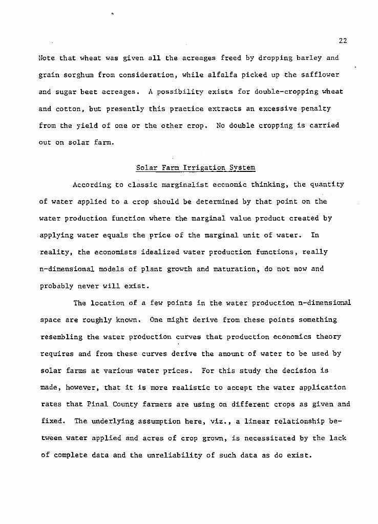
Note that wheat was given all the acreages freed by dropping barley and
grain sorghum from consideration, while alfalfa picked up the safflower
and sugar beet acreages. A possibility exists for double-cropping wheat
and cotton, but presently this practice extracts an excessive penalty
from the yield of one or the other crop. No double cropping is carried
out on solar farm.
Solar Farm Irrigation System
According to classic marginalist economic thinking, the quantity
of water applied to a crop should be determined by that point on the
water production function where the marginal value product created by
applying water equals the price of the marginal unit of water. In
reality, the economists idealized water production functions, really
n-dimensional models of plant growth and maturation, do not now and
probably never will exist.
The location of a few points in the water production n-dimensional
space are roughly known. One might derive from these points something
resembling the water production curves that production economics theory
requires and from these curves derive the amount of water to be used by
solar farms at various water prices. For this study the decision is
made, however, that it is more realistic to accept the water application
rates that Pinal County farmers are using on different crops as given and
fixed. The underlying assumption here, viz., a linear relationship be
tween water applied and acres of crop grown, is necessitated by the lack
of complete data and the unreliability of such data as do exist.
23
The total water requirement of solar farm was determined using
coefficients that linked acres of crops grown to specific amounts of
water applied. Two sources of such coefficients exist. The first source
is Arizona Agriculture Experiment Station (1968) which gives plant con
sumptive need by semimonthly period. These figures establish useful
minimums for allocating water by semimonthly periods; however, lacking
knowledge of farm water application efficiency, i.e., the percentage of
irrigation water delivered from the well that is stored in the soil for
consumptive use by crops after allowing for irrigation losses, they are
of little value for determining total solar farm pumpage.
In order to determine solar farm pumpage, data from Hathom et al.
(1976) were used. This report is one product of an extensive farm manage
ment information system (MIS) that has been developed at The University of
Arizona. This MIS is based on data collected from farmers, extension
agents, and other experts in the industry infrastructure. The informa
tion is updated yearly. One type of information collected from the
Pinal budgets is how much water farmers pump for crops and when. It was
this information, refined by plant consumptive use data, that was used
as the basic water demands on which this report is based.
Tables 4 and 5 show the per acre and total water applications for
each of the four crops used in this study for every semimonthly period.
Alfalfa production requires 729 acre-feet, cotton 2,396 acre-feet and
wheat 1,317 acre-feet annually. The total pumpage required on the solar
farm is 4,450 acre-feet. The highest monthly total pumpage is 609 acre-
feet in April and the highest semimonthly total is 335 acre-feet in late
May. Satisfaction of the semimonthly pumpage requires the greatest
24
Table 4. Solar Farm Crop Water Application Pattern — Water Used per Acre in Acre-inches.
Semi-MonthlyPeriod
AlfalfaEstablishment Alfalfa Upland
CottonPimaCotton Wheat
JanuaryEarly — — 12(4) — —
Late — — — — 8(.5)February
Early — 5 12(.15) — —
Late — — 12( .15) 12 —
MarchEarly — 5 12(.3) — —
Late — — — — 7.5CApril
Early — 5 — — 7.5Late — 5 — — 7.5
May.Early — 5 — — 6Late — 5 6 6 1.5
JuneEarly — 6 6 6 —
Late — 6 6 6 —
JulyEarly — 6 6 6 — —
Late — — 6 6 6 —
AugustEarly — 6 6 6 —
Late — — 6 6 —
SeptemberEarly — 5 6 6 — —
Late 12(,5)/4(.5) — 6 6 —
OctoberEarly 12(.5) 5 — — 6 — —
Late 4(.5) — — — — —
NovemberEarly 4( .5) 5 — — — —
Late — — — — —
DecemberEarly 4(.5) — — — — — — — —
Late — — — — 8(.5)TOTALS 20.0 75.0 60.0 66.0 38.0
25
Table A. (continued)
a. Alfalfa is a three-year crop; one-third of stand establishment has been charged to each year.
b . "(.X)" indicates proportion of crop irrigated during period.
c. Wheat irrigation shifted toward first half of growing season. No stress of plant should result.
26
Table 5. Solar Farm Crop Water Application Pattern — Total Water Used in Acre-feet.
a. Upland cotton pre-irrigation has been scheduled from early January to early March so as to smooth pump demand.
b. The annual total pumpage for the entire farm is 4,449 acre-feet; the highest monthly pumpage is 609 acre-feet for April and highest semi-monthly pumpage is 335 acre-feet in the late May period.
amount of pumping, and so, determines the total well capacity needed on
solar farm.
A word of explanation is in order concerning the reason the
monthly maximum pumpage occurs in April. The current situation on most
Pinal County farms is, of course, that irrigation demand is the highest
in the summer since the maximum cotton irrigating requirements occur
during this season. Cotton is the major Pinal County crop. For solar
farm, however, cotton and wheat production will be, as noted earlier, of
about equal importance. Cotton and wheat both require irrigation in
late May, and it would be very expensive to build a system to satisfy
the Hathom irrigation schedule for both crops. Fortunately, this prob
lem can be lessened by shifting the wheat irrigation schedule so that
this crop is watered more heavily earlier in the year than is the current
practice. In fact, judged in terms of satisfying the consumptive need
of wheat for water, such a shift from current practice improves the ir
rigation schedule (see Table 6). Table 6 shows the changes in irrigation
schedule made for this study. Since wheat still receives in total as
much water as called for by the existing schedule, this adjustment should
be costless, and since reducing late May irrigation permits the farmer to
get by on a lower well-field capacity, he will be motivated to make such
a shift to reduce fixed costs. In the case of solar farm this simple ad
justment allows two 1,200 gpm wells to be removed from the farm structure
at a saving in capital investment of about $150,000.
Knowing plant water consumptive demands and water supplied, it is
possible to derive the irrigation efficiencies implicit in the Hathom
budget (see Table 7). The efficiencies shown in Table 7 for cotton or
Percent of Total Water Provided 36.4 29.4 22.4 11.9
a. Figures shown are days operated during period to meet water requirement .15- day capacity = 79.5 acre-feet/well16- day capacity = 84.8 acre-feet/well 365-day capacity = 1934.5 acre-feet/well 1200 gpm wells supplying 5.3 acre-feet/day
37
Table 10. Cost of Pumping Water in 1976, Well No. 1.
WELL NO 1SOLAR FARM 3ASE CASE
ELECTRIC POWERPINAL COUNT?
460 FOOT LIFT
A. SPECIFICATIONS AND ASSUMPTIONSk3.iiJ:11#
VITH 16 LSCH CASINC ro 1500 FEET c1 ? annually
0EPRECIATEFw ELLN25 YEARS'WITN^^O^PERCENT SALVAGE OEPRECIATe PUMP ASSEMBLY 25 YEARS WITH 3 PERCENT SALVAGEW A l t i m 5838 8S1?e55sy§8S vr^ERh5lRlK!?A!lLVAGECOMPUTE INTEREST ON AVERAGE INVESTMENT AT 8.50 PERCENT COMPUTE TAXES ON 18.00 PERCENT OF AVERAGE INVESTMENT USING A TAX RATE OF 510.21 PER $100 ASSESSED VALUATION
3. PRICE QUOTATIONS (INCLUDING 4.0 PERCENT SALES T A X ) -- 02/31/761.i:4.5.6.7.
r a § sf35fci h! m 8d?iu"“'POWER UNIT-- 250 HP MOTORSTARTER VITH HAND COMPENSATOR ANDi«fS£?S?{85 ESbSS SVITCHC.
0.
TOTAL COST OF WELL ANNUAL FIXED COSTS
^ I i S ATriQNTAXESFIRE AND LIGHTNING INSURANCE TOTAL
WATER COST PER ACRE FOOT 1. FIXED COST
VARIABLE COST
24000.15251.19009.3536.5 30 2*1313.
74547.
2.7002./1619.
♦ 460(1.02414.33AF*
lit?:695 • 154.7002.
■ 4.32.01200)/.520
WHERE 1.024460.01200.520.007512
+ .007512 ♦ 460 AT 100
POWER COST PER KWH INCLUDING SALES TAX OVERALL EFFICIENCY STATED AS A DECIMAL FRACTION COST OF PLANT REPAIRS, MAINTENANCE, LUBRICATION AND ATTENDANCE PER FOOT OF LIFT
E.3.KWH
TOTAL COST » 18.65OF ELECTRICITY USED TO PUMP 1 AF 905.85 1619 AF * 1466565.
38
Table 11. Cost of Pumping Water in 1976, Well No. 2.
WELL NO 2 ELECTRIC POViER_SOLAR_FARM 3a 3E CASE PINAL COUNTY
SPECIFICATIONS AND ASSUMPTIONS
460 FOOT LIFT
1.2.3.4.5.*:9.xS:11.
>/ElL IS DRILLED AND CASED WITH 16 INCH CASING TO 1500 FEET 90<LS ARE SET AT 500 FcET
DEPRECIATE W E L L E S YEARs'°IT4*^0*PERCENT SALVAGE DEPRECIATE PUMP ASSEMBLY 25 YEARS WITH 3 PERCENT SALVAGEoIprIciat! m T P E R & s M ^ r ^COMPUTE INTEREST ON AVERAGE INVESTMENT AT 8.50 PERCENT COMPUTE TAXES ON 13.00 PERCENT OF AVERAGE INVESTMENT USING A TAX RATE OF $10.21 PER $100 ASSESSED VALUATION
& i 5 M ! N rilL,T,0S!S"5»)Ssi8:t5 !u WSSeSfi"'"'POWER UNIT-- 250 HP MOTORSTARTER «ITH HAND COMPENSATOR ANDtNSfS£S!?!85 ISSSS SU,TCH
0.
TOTAL COST OF WELLANNUAL FIXED COSTS
DEPRECIATION 2940.INTEREST 3213.TAXES 695.FIRE ANO LIGHTNING INSURANCE 154.TOTAL 7002.
WATER COST PER ACRE FOOT1. FIXED COST « 7002./1307.2. VARIABLE COST » (1.024 * 460
AF ■ 5.36* .01200)/.520• 14.33
24000.15251.19009.3536.6136.5302.1313.
74547.
♦ .007512 + 460
UMERE 1-°60 ! “";%EJfIoiEi4iSFE I?hJc5OOT AT100♦ 01200 » POWER C O S T N E R KWH INCLUDING SALES TAX.520 » OVERALL EFFICIENCY STATED AS A DECIMAL FRACTION .007512 ■ COST OF PLANT REPAIRS# MAINTENANCE, LUBRICATIONANO ATTENDANCE PER FOOT OF LIFT
3. TOTAL COST - 14.69E. KWH OF ELECTRICITY USED TO PUMP 1 AF • 905.35 1307 AF • 1183941.
39
Table 12. Cost of Pumping Water in 1976, Well No. 3.
WELL MO 3SOLAR FARM BASE CASE
ELECTRIC POWERPINAL COUNTY
460 FOOT LIFT
A. SPECIFICATIONS ANO ASSUMPTIONS1. WELL IS DRILLED AND CASED WITH 16 INCH CASING TO 1500 FEET2. BOWLS ARE SET AT 500 FEET3. WELL PUMPS 1200 GPM AND 995 ACRE FEET ANNUALLY4. ELECTRICTY COST IS 12.00 MILLS PER KWH5. OVERALL EFFICIENCY IS 52.0 PERCENT6. DEPRECIATE WELL 25 YEARS WITH 0 PERCENT SALVAGE7. DEPRECIATE PUMP ASSEMBLY 25 YEARS WITH 3 PERCENT SALVAGE9. DEPRECIATE POwER UNIT 25 YEARS WITH 3 PERCENT SALVAGE8. DEPRECIATE BOWLS 25 YEARS WITH 3 PERCENT SALVAGE10. COMPUTE INTEREST ON AVERAGE INVESTMENT AT 8.50 PERCENT11. COMPUTE TAXES ON 18.00 PERCENT OF AVERAGE INVESTMENT USINGA TAX RATE OF $10.21 PER $100 ASSESSED VALUATION
a. PRICE QUOTATIONS «INCLUDING 4.0 PERCENT SALES TAX) -- 02/31/76«l!S§Ai3S«LL1Tlra1.2.3.3:6.
7.
PUMP ASSEMBLY ( 3 INCH COLUMN)12 INCH BOWLS (11 STAGES)POWER UNIT-- 250 HP MOTORSTARTER WITH HAND COMPENSATOR ANDSECONDARY POWER STATION WITH SAFETY SWITCH INSTALLATION LABOR AND SITE COSTSTOTAL COST OF WELL
ANNUAL FIXED COSTSDEPRECIATIONINTERESTTAXESFIRE AND LIGHTNING INSURANCE
TOTALWATER COST PER ACRE FOOT
24000.15251.19009.3536.6136.5302.1313.
74547.
ISiS:695.154.7002.
1.2.
FIXED COST VARIABLE COST
7002./ 995. AF « 7.04(1.024 ♦ 460 * .01200)/.52014.33
WHERE 1.024460.01200.520.007512
+ .007512 * 460100KWH TO LIFT 1 AF OF WATER 1 FOOT AT
FEET OF LIFTVERALL EFFICIENCYPOWER COST PER KWH INCLUDING SALES TAX OVERALL EFFICIENCY STATED AS A DECIMAL FRACTION COST Oh PLANT REPAIRS, MAINTENANCE, LUBRICATION AND ATTENDANCE PER FOOT OF LIFT
E.3. TOTAL COST • 21.37KWH OF ELECTRICITY USED TO PUMP 1 AF * 905.85 995 AF ■ 901317.
40
Table 13. Cost of Pumping Water in 1976, Well No. 4.
WELL NO 4 ELECTRIC POWER__ SOUR_FARM BASE CASE PINAL COUNTYA . SPECIFIC A H 0NS~AN0~AS SUMPTIONS
460 FOOT LIFT
1.2.3.t:b7\a9:H:
E.
SSits'hi’ikV'S/SSo'Hi?11 "" CASIHS T" 1510 fEET l E S r H S ' T M i S ? 3f?L5c5!.Fl55 ‘•'"( U 1 U Y0EPRE^ATErWELLN 25 YEARs'wiTH*^O^PERCENT SALVAGEW?llcch\l" --- 25 YEARS WITH 3 PERCENT SALVAGEON AVERAGE INVESTMENT AT 8.50 PERCENT 18.00 PERCENT OF AVERAGE INVESTMENT USING $10.21 PER 1100 ASSESSED VALUATIONDEPRECIATE BOWLS COMPUTE INTEREST COMPUTE TAXES ON A TAX RATE OF
PUMP ASSEMBLY ( 8 INCH COLUMN)12 INCH BOWLS (11 STAGES)POWER UNIT-- 250 HP MOTORSTARTER WITH HAND COMPENSATOR ANDi«?I£SI?i35 ESiSSS !Mrs!TEwcasTi1FElr SUITCH
TOTAL COST OF WELL ANNUAL FIXED COSTS
24000.15251.19009.3536.6136.5302.1313.
74547.
TAXESFIRE AND LIGHTNING INSURANCE29403lhl154
t o t a l 7002WATER COST PER ACRE FOOT1. FIXED COST - 7002./ 529. AF » 13.2. VARIABLE COST 1 (1.024 * 46014.33 * .01200)/ + .007512 * 460
100WHERE u ;6z; ; ; ; % % ^ E ^ L r E F ^ i c E!Eic?ooT AT.01200 * POWER COST PER KWH INCLUDING SALES TAX
3. TOTAL COST * 27.57KWH Or ELECTRICITY USED TO PUMP 1 AF » 905.85 529 AF - 479193.
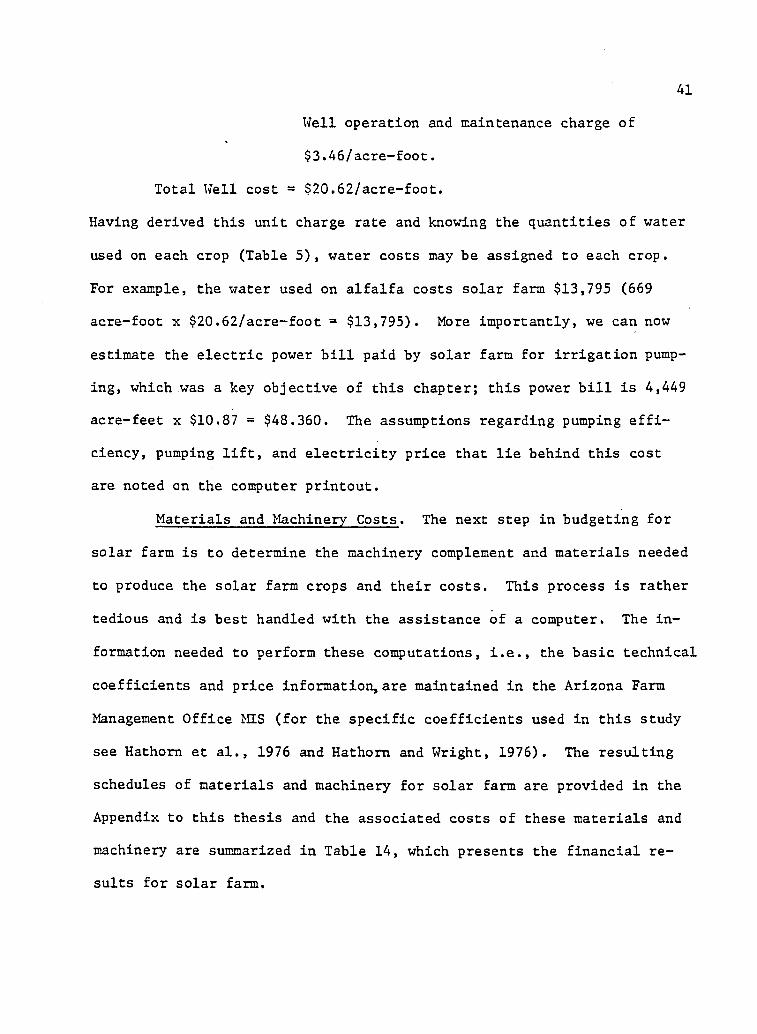
Well operation and maintenance charge of
$3.46/acre-foot.
Total Well cost = $20.62/acre-foot.
Having derived this unit charge rate and knowing the quantities of water
used on each crop (Table 5), water costs may be assigned to each crop.
For example, the water used on alfalfa costs solar farm $13,795 (669
acre-foot x $20.62/acre-foot = $13,795). More importantly, we can now
estimate the electric power bill paid by solar farm for irrigation pump
ing, which was a key objective of this chapter; this power bill is 4,449
acre-feet x $10.87 = $48,360. The assumptions regarding pumping effi
ciency, pumping lift, and electricity price that lie behind this cost
are noted on the computer printout.
Materials and Machinery Costs. The next step in budgeting for
solar farm is to determine the machinery complement and materials needed
to produce the solar farm crops and their costs. This process is rather
tedious and is best handled with the assistance of a computer. The in
formation needed to perform these computations, i.e., the basic technical
coefficients and price information, are maintained in the Arizona Farm
Management Office MIS (for the specific coefficients used in this study
see Hathorn et al., 1976 and Hathom and Wright, 1976). The resulting
schedules of materials and machinery for solar farm are provided in the
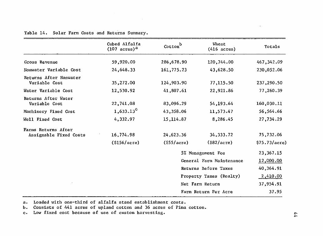
Appendix to this thesis and the associated costs of these materials and
machinery are summarized in Table 14, which presents the financial re
41
sults for solar farm.
Returns
42
The solar farm described here earns a net return of $37,955 or
$37.95 per cropped acre after management fees and taxes and $75.73 per
cropped acre before these whole-farm costs are netted out. There is in
sufficient information to compute a rate-of-return on investment. Al
falfa returns $156/cropped acre, wheat $82/cropped acre and cotton $55/
cropped acre. Irrigation related costs, which include not only the cost
of the water but also that of the labor in setting up for each irrigation
run are proportionately higher for alfalfa than cotton or wheat; that is,
the ratio of irrigation costs to all assignable costs is higher for al
falfa (.39) than for either wheat (.27) or cotton (.22). This ratio
could be used as an index of the sensitivity of each crop to rising water
prices. Irrigation-related costs, however, do not dominate the farm
balance sheet. They are an important decision variable for the farm,
but not the only decision variable. This point is important to remember
when predicting farm adjustments to rising well level water prices, which
are, themselves, only a subset of irrigation costs.
The high level of returns on alfalfa may be caused by the assump
tion that on solar farm the alfalfa crop is watered sufficiently to ob
tain maximum physical yield. This assumption results from using the Farm
Management MIS budgets. According to the Arizona Farm Management Office,
Arizona farmers quite often stress alfalfa by cutting off water to it
during those summer months when it is competing with cotton for water.
The effect of this practice is reflected in the fact that the solar
farm's yield on alfalfa per year is 7 tons/acre (Hathorn et al., 1976) while in 1975 the Pinal County average yield was 6 tons/acre (Arizona
Crop and Livestock Reporting Service, 1976). At 6 tons/acre the alfalfa
return per acre would drop from $156 to $77, which is in line with the
returns on wheat and cotton. See Table 14 for solar farm summaries.
Farms Returns After Assignable Fixed Costs 16,774.98 24,623.36 34,333.72 75,732.06
($156/acre) ($55/acre) ($82/acre) $75.73/acre)
5% Management Fee 23,367.15General Farm Maintenance 12,000.00Returns Before Taxes 40,364.91Property Taxes (Realty) 2,410.00Net Farm Return 37,954.91Farm Return Per Acre 37.95
a. Loaded with one-third of alfalfa stand establishment costs.b. Consists of 441 acres of upland cotton and 36 acres of Pima cottonc. Low fixed cost because of use of custom harvesting. -O
CHAPTER III
DETERMINATION OF ECONOMICALLY JUSTIFIABLE INITIAL COST OF SOLAR SYSTEM
In this chapter, the total initial cost of a solar-thermal genera
tion plant economically justified by changes in solar farm annual oper
ating costs will be determined. It will be assumed throughout that all
energy for pumping groundwater will be supplied by the solar plant. If
for whatever reason this assumption does not hold, the justified initial
cost of the solar plant must be reduced in proportion to the share of
total groundwater pumping energy that is supplied by the solar equipment.
Computational Approach
Basically, the computational procedure followed in this chapter
will be to isolate the cost of electrical energy for irrigation pumping
out of total farm cost and to convert this constant annual cost stream
to its present value equivalent. This present value figure represents
for solar farm the maximum justifiable investment in solar equipment that
frees solar farm from the need to purchase electricity. Note that "jus
tified investment" is not the same as "justified initial cost"; this dis
tinction will become clear shortly. At the present stage in the develop
ment of solar power, it is felt to be purposeless to consider the effect
of such changeable policy items as accelerated depreciation rules and
special investment credits on the solar investment decision. To some ex
tent the effect of policy variables are represented by including differ
ent discount rates. To give the following results as broad an
45
applicability as possible, investment levels will be computed over a
wide range of pumping lifts and pumping efficiencies.
A basic solar thermal plant will be described in Chapter IV. At
this stage of the analysis, however, some idea of how a solar plant oper
ates must be introduced. A solar thermal electric plant has two major
sections. The first section, termed the collector, gathers the diffuse
incoming radiant energy of sunlight and concentrates it to the high levels
needed for generating electricity efficiently. At the present time there
are several ways that seem possible for doing this energy collection job;
the one we have assumed for this study is called a central-tower collector.
In the central tower collector, special mirrors focus solar energy onto a
central tower through which a fluid is passed. This fluid collects the
focused solar energy in the form of heat. Collector technology for
thermal-electric plants is mostly unproven. We will assume an operational
life of 15 years for this section of the solar-thermal plant.
The second section of the solar-thermal plant generates the elec
tricity from the heated fluid. The technology for doing this job is well
understood; the main questions revolve around the method for generating
the electricity most efficiently at the relatively low working fluid
enthalpies expected. Electrical generation equipment is commonly assumed
to have an operational life of 30 years.
Because the two sections of the solar plant have distinctly dif
ferent operational lives, some scheme must be derived for dividing the
justified investment between the collector section and the generating sec
tion. The planning horizon of the solar plant will be taken at 30 years.
During this time, the solar farm must purchase one generating section and
46
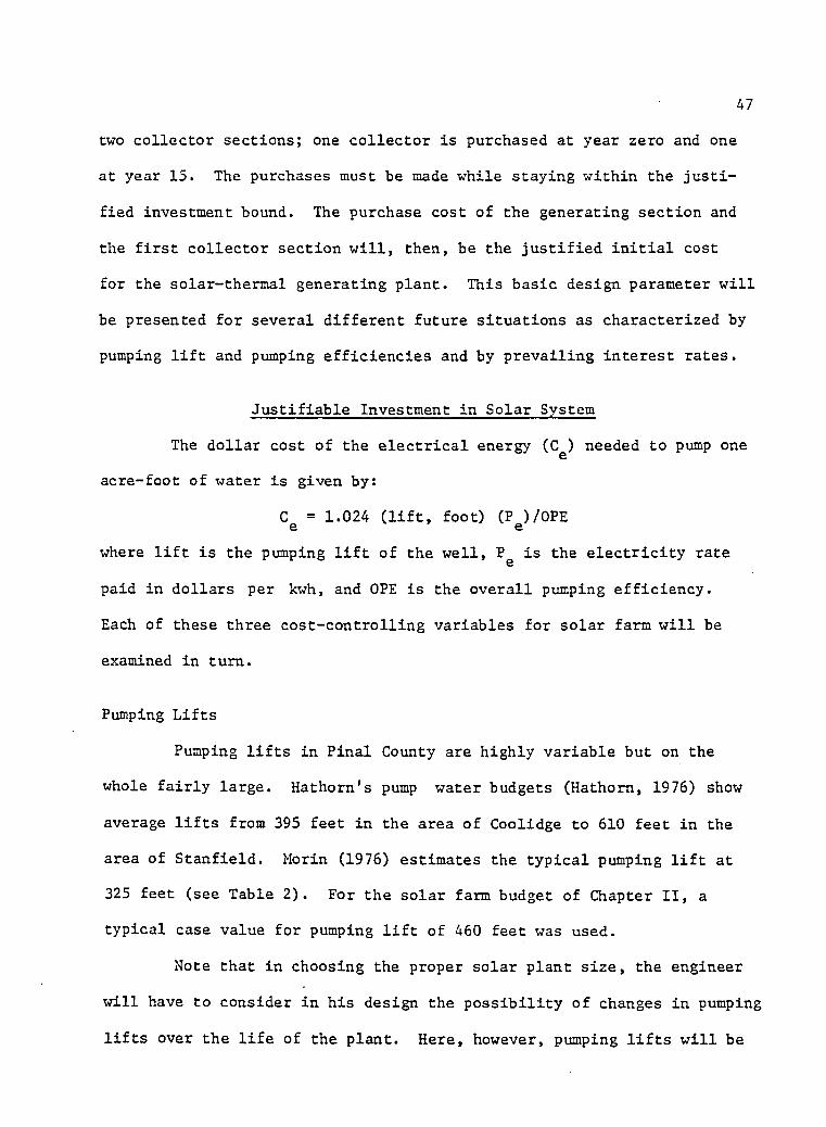
47
two collector sections; one collector is purchased at year zero and one
at year 15. The purchases must be made while staying within the justi
fied investment bound. The purchase cost of the generating section and
the first collector section will, then, be the justified initial cost
for the solar-thermal generating plant. This basic design parameter will
be presented for several different future situations as characterized by
pumping lift and pumping efficiencies and by prevailing interest rates.
Justifiable Investment in Solar System
The dollar cost of the electrical energy (C^) needed to pump one
acre-foot of water is given by:
C = 1.024 (lift, foot) (P )/OPE e ewhere lift is the pumping lift of the well, P^ is the electricity rate
paid in dollars per kwh, and OPE is the overall pumping efficiency.
Each of these three cost-controlling variables for solar farm will be
examined in turn.
Pumping Lifts
Pumping lifts in Pinal County are highly variable but on the
whole fairly large. Hathorn's pump water budgets (Hathorn, 1976) show
average lifts from 395 feet in the area of Coolidge to 610 feet in the
area of Stanfield. Morin (1976) estimates the typical pumping lift at
325 feet (see Table 2). For the solar farm budget of Chapter II, a
typical case value for pumping lift of 460 feet was used.
Note that in choosing the proper solar plant size, the engineer
will have to consider in his design the possibility of changes in pumping
lifts over the life of the plant. Here, however, pumping lifts will be
48
looked at as holding constant for solar farm over the entire operating
life of the solar plant. Grant and Ireson (1970, p. 42) show that a
gradient, i.e., arithmetic, series of constant increases, G, over n years
can be converted to an equivalent constant annual figure, A, by the
expression:
A = Gi
nGi (1 + i)n - 1
where i is the discount rate. For example, say pumping lift is increasing
at 8.1 feet/year, which according to the Arizona Water Commission (1975)
is the typical annual fall in the water table in Pinal County. For a
discount rate of 8.5% and a planning horizon of 30 years, A is given by
a = (8.1) _ 30 (8.1).085 .085
.085(1.085)30 - 1
= 72.3 feet
Thus, a 460 foot constant lift for 30 years would be economically equiva
lent to a situation where the lift in the first year was 387.7 feet,
rising in 8.1 foot increments to 626.6 feet by the thirtieth year.
Electricity Prices
The price of electrical energy at various locations in Pinal
County given in the Hathom budgets (Hathom, 1976) is as follows:
Coolidge 12 mills/kwh
Casa Grande 12 mills/kwh
Eloy 11 mills/kwh
Stanfield 26.3 mills/kwh
Maricopa 13.5 mi11s/kwh
For the solar farm base case a typical energy price of 12 mills/kwh was
chosen.
Pinal County electricity prices are unusual in two respects. The
first respect in which the prices are unusual is that the electric dis
tricts^ serving Pinal County farmers charge one flat rate no matter how
much electricity is consumed. More typically in Arizona a declining
block rate pricing schedule is used. Fuel adjustments and taxes are
overlain on this schedule. For example, the two largest utilities in
the state, Arizona Public Service and Tucson Gas and Electric, both use
the declining block rate method. Also, both weight the block prices by
the peak potential demand of the well as measured by the size of the electric motor being served.
The second respect in which Pinal County electricity prices are
unusual is that relative to other prices for similar service, they are
very low. Nationwide the cost of electricity generation is typically
20 to 25 mills/kwh (Conn and Kulcinski, 1976). No other area of Arizona
enjoys prices as low as those seen in Pinal County. The highest elec
tricity price for irrigation service at the time of the writing of this
thesis is the 40.15 mills/kwh Tucson Gas and Electric charges for its
first block. Typical Arizona 1975 electricity prices in other counties
work out to flat rate equivalents of from 23.0 to 27.7 mills/kwh (Hathom,
1976). Pinal County electricity prices are low seemingly because the
electric districts were able to obtain long tern contracts for large
amounts of cheap hydroelectric power. According to Hathorn, these sup
ply contracts will typically remain in force for another decade.
1. Electrical districts are electrical retailing cooperatives run in the interest of local agricultural and other users.
49
50Overall Pumping Efficiency
The overall pumping efficiency parameter measures how well the
motor and pump are doing their work. OPE, like pumping lift, shows a
wide range of values in the field. To a certain extent, the OPE level
is under the control of the farmer through maintenance and replacement.
For the solar farm base case the typical OPE was set at .54. This value
will probably become lower than typical as energy prices move up; how
ever, the leeway in optimizing pumping efficiency is not great enough to
counteract very large electricity price rises or pumping lift increases.
The theoretical maximum OPE is about .75 (Nelson and Busch, 1967).
Electricity Cost Computation
Electricity costs for solar farm are computed in Table 15 for the
base case and some variational cases. The high OPE of .66 used in the
table was picked as the highest OPE level that could be maintained on an
irrigation well for a year. Note from the table that the farmer could
maintain the same level of electricity costs up to a depth of 560 feet
by adjusting the OPE but that beyond this depth the electricity bill will
begin to rise. The typical case figure of $46,580 represents about 11%
of the total solar farm costs.
It should be noted here that solar plants may have another effect
than just merely ending the annual stream of farm electricity purchases.
It seems fairly certain that additional annual operation and maintenance
charges will result for the solar farm. There is even some likelihood
that solar plants will require fulltime attendance. Whatever these addi
tional O&M charges may be, the potential annual cost savings from using
51
Table 15. Annual Costs of Electricity to Solar Farm.3,
O v e r a l l ________________ Pumping Lift (feet)PumpingEfficiency
Very Shallow (200)
Shallow(360)
Typical(460)
Deep(560)
Low (.42) $26,038 $46,869 $59,889 $72,908
Typical (.54) $20,252 $36,454 $46,580 $56,707
High (.66) $16,570 $29,826 $38,111 $46,397
a. 4,450 acre-feet annual pumpage; price of electricity is 12 mills/kwh.
52
solar power would have to be adjusted downward for them. The same cau
tion also applies to the results shown in the following two tables. For
example, if the additional farm O&M from a solar plant is $16,700 per
year, for an efficient well with a 200-foot pumping lift, there are an
nual disbenefits of $130 ($16,570 - $16,700) to using solar power on the
farm (see Table 15). Estimates of how much O&M will cost for solar
plants at this point in the development of solar power are purely guess
work, but it will clearly be seen during the development of this chapter
how vital it is to the feasibility of using solar power for irrigation
pumping that this parameter be kept as low as possible.
Present Worth Computation
The present worth factor for determining the present value of an
annual series of payments (P/A) is derived in most beginning engineering
economics texts (see, for example, Grant and Ireson, 1970). It is:
(P/A)(1 -f i)n - 1 i (1 + i)n
Here i represents an assumed constant interest, or discount, rate and n
represents the number of interest periods. The number of interest peri
ods will be taken to be the number of years in the operational life of
the solar-thermal plant, 30 years.
The i variable in this equation is the long-term opportunity
price of money to the farmer. If society undertakes to encourage solar-
energy use for extra economic reasons, the opportunity price of money
used to purchase solar equipment seen by the farmer might be quite low,
say about 4%. On the other hand, without loan guarantee programs,
53
farmers may have a difficult time arranging the financing needed for the
new, unproven solar technology from risk averse investors and might have
to pay a risk premium, raising i up to, say, 13%. The solar farm will be
assumed to be able to obtain funds for the solar equipment at 8.5%. (The
Farm Administration (U. S. Department of Agriculture, 1975) states that
interest rates on agricultural loans stood at between 8.5% and 9% on
June 30, 1975).
Table 16 shows the justified investment levels for discount rates
of i = .04, .085, and .13. The values are computed by multiplying the
present worth factor by the annual costs of electricity computed in Table
15. For the typical case (lift = 460 feet, OPE = .54, i = .085) the
justified investment is about one-half million dollars over the 30-year
project period.
Justifiable Solar System Initial Cost
The justified initial cost for the solar plant is estimated by
apportioning the justified investment derived in the previous section be
tween the collector and generating sections of the solar plant. This
must be done so that, first, sufficient investment "funds" are retained
after the initial purchase to purchase a second collector section at 15
years, and that secondly the ratio between the capital costs of the col
lector and the generating section is maintained at 3:1. (This estimate
or cost proportions is based on discussions with Larson (1976) and Sands
(1976) . The "justified initial cost" is the delivered and operating
costs for a solar plant at year zero. It does not include the cost of
the later collector. It should include adjustment for the additional
54
Table 16. Justified Investment in Solar Equipment for Various Values of Pumping Lift, Pumping Efficiency, and Discount Rates (1976 dollars).
55operation and maintenance annual cost streams that are introduced on the
farm by the solar plant.
Justifiable Cost before O&M Charges
As we have noted earlier, fixed electrical generation equipment
typically is expected to have an operational life of around 30 years.
On the other hand, the solar collector section of solar-thermal genera
tion plant, which both requires untried technology and which will neces
sarily be subjected to a somewhat severe physical environment, has been
assumed to have an operational life only half that of the generating sec
tion. Accurate estimates of operating life prepared in advance of actual
experience with the collector equipment are very difficult to make.
To satisfy the electrical demands of farms similar to the solar
farm described in Chapter II, farms ranging in size from roughly 200 to
2,000 irrigated acres requires solar-thermal plants of from 1 to 10 1OT .
("MW^" means megawatts-thermal and refers to the maximum rate heat is
generated within the solar plant; this parameter can be used to charac
terize the plant capacity as can "kw^," or kilowatts-electric, which
refers to the power output of the plant.) For such plants it is esti
mated that three-fourths of the initial capital costs will be spent on
the shorter-lived collector section.
The basic present value problem is somewhat complicated here by
the fact that the collector section of the solar suite only operates for
15 years. If solar farm were to spend all its justified investment from
Table 16 immediately, the solar plant would operate for only 15 years.
After the 15 years were up, solar farm would be left with an inoperable
56
collector hooked up to a still operable electrical generation system. No
further investment could be justified for replacing the solar collector.
So, the problem is to determine how much of the total justified invest
ment capital can be invested in a generator and collector, that is in a
solar plant, at the start of the project and how much of it should be
conserved for purchase of a second solar collector 15 years into the
project.
Looked at from a different point of view, solar farm may not use
all of the justified investment at the start of the project because if it
did it would again be faced with paying for off-the-farm electricity be
tween the fifteenth and thirtieth year of the project. This would vio
late the assumption under which justified investment was computed. Since
it may not "invest" all of the stream of electricity costs in solar
equipment initially, it in effect has a stream of savings for the first
fifteen years, and it then invests this money (principal and interest) at
the fifteenth year in the second collector section.
Let Cc be the justified initial cost for the collector section
and Cg be that of the generating section of the solar plant. The total
justified initial cost for the solar plant is:
C = C + Ct e gFrom the present worth factor and the constant annual solar farm elec
tricity costs over 30 years the upper bound on current solar investment
has been computed; call this is the maximum amount of capital
solar farm can justifiably commit to the purchase of a solar system over
the 30-year project and still leave its financial position unchanged.
It is assumed that solar farm will pay the same amount at the
start of the project for a collector as it pays in the fifteenth year,
that is, that the cost of the collector does not change with time. The
amount of the justified investment not spent at the start of the project
(It - C^), that is, the amount conserved for purchase of the second col
lector, together with its compounded interest, is made to equal the
justified cost of the collector section at the fifteenth year, that is:
cc = (it - ct) (i + i)15 = (it - [cc + cg]) (i + i)15It was estimated that the ratio between the initial cost of the collector
section and of the generating section is 3:1, or C = 1/3 C ; substituting8 cthis expression into the above equation results in:
Cc = (It - [4/3] Cc) (I + i)15,and, solving for C^:
Cc + (4/3) Cc (1 + i)15 - Ic (1 + i)13
Cc = It (1 + i)15 / (1 + [4/3] [1 + i]15)
Since 1^ is known from Table 16, may be computed. With known the
values of Cg and quickly follow. The results of this computation are
shown in Table "17.
The figures in Table 17 estimate the level of initial cost the
solar system designer will have to meet to compete with conventional
energy pumping systems for farms operated similarly to solar farm. The
most likely "future states" lie along the diagonal running from the
upper left to the lower right of the table. As expected, the results
show the following: the more efficient the farm wells, the less the
justified initial cost level for solar; the higher the interest rate, the
less the initial cost; and the greater the pumping lift the greater the
57
Table 17. Justified Initial Costs for Collector Section, Generator Section, and Total Solar Power Plant for Solar Farm Financial Breakeven in Thousands of 1976 Dollars.a
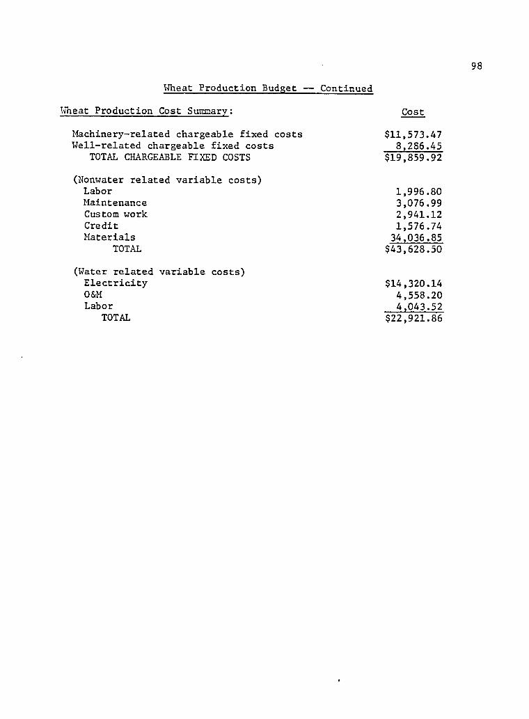
(Nonwater related variable costs)Labor 1,286.09Maintenance 479.36Short-term credit 389.81Custom work 19,110.20Materials 3,383.20
TOTAL $24,648.33
(Water related variable costs)Electricity 7,487.98
2,383.482,659.46
TOTAL $12,530.92
LIST OF REFERENCES
Arizona Agriculture Experiment Station, Consumptive use of water by crops in Ariozna, The University of Arizona, Tucson, Technical Bulletin 169 (reprint), August 1968.
Arizona Bureau of Mines, Mineral and water resource of Arizona, Bulletin 180, Tucson, Arizona, 1969.
Arizona Crop and Livestock Reporting Service, 1975 Arizona Agricultural Statistics, Bulletin S-ll, Phoenix, Arizona, March 1976.
Arizona Water Commission, Summary: Phase I — Arizona state water plan,inventory of resource and uses, Phoenix, Arizona, July 1975.
Conn, Robert W. and Gerald C. Kulcinski, Fusion reactor design studies. Science, 193:4254, August 20, 1976.
Firch, Robert, Professor, Department of Agricultural Economics, The University of Arizona, Tucson, personal communication, 1974.
Frank, Helmut, in Arizona Statistical Review, Valley National Bank of Arizona, Phoenix, 31st ed., p. 38, September 1975.
Grant, Eugene L. and W. Grant Ireson, Principles of engineering economy, (5th ed.), The Ronald Press Co., New York, 1970.
Hathom, Scott, Jr., Arizona pump water budgets, Pinal County 1976,Department of Agricultural Economics, The University of Arizona (analogous reports are issued for Pima, Cochise, and Maricopa Counties), February 1976.
Hathom, Scott, Jr., Charles Robertson, James Little and Sam Stedman, 1976 Arizona field crop budgets, Pinal County, Department of Agricultural Economics, The University of Arizona, Tucson,April 1976.
Hathom, Scott, Jr. and N. Gene Wright, Arizona farm machinery costsfor 1976, Department of Agricultural Economics, The University of Arizona, Tucson, January 1976.
Joskow, Paul L. and Martin L. Baughman, The future of the U. S. nuclear energy industry. The Bell Journal of Economics, Vol. 7, No. 1, Spring 1976.
Larson, Dennis, Professor, Department of Soils, Water and Engineering,The University of Arizona, Tucson, personal communication, 1976.
101
102
Manne, Allen S ., Electricity investments under uncertainty: waiting forthe breeder, in Energy: Demand, Conservation and InstitutionalProblems, Michael S. Maerakis, Ed., MIT Press, Cambridge, Massachusetts, 1973.
Morin, George, Lecturer, Department of Soils, Water and Engineering, The University of Arizona, Tucson, personal communication, 1976.
Nelson, Aaron G. and Charles D. Busch, Cost of pumping irrigation water in central Arizona, Arizona Agriculture Experiment Station, Technical Bulletin 182, The University of Arizona, Tucson,April 1967.
Ozsabuncuoglu, Ismail, Economic impacts of alternative irrigation systems under increasing irrigation water costs in southwestern Arizona, Doctoral dissertation in preparation, Department of Agricultural Economics, The University of Arizona, Tucson, 1976.
Sands, Charles D., II, Research Associate, Department of Soils, Water and Engineering, The University of Arizona, Tucson, personal communication, 1976.
Strickland, James H., Merton E. Fewell, Steven 0. Heard, Prashant D.Parikh and Thomas E. Burnette, The on-site utilization of solar energy for agricultural operations in Texas, Prepared for the Office of the Governor under contract GAEC IAC (76-77)-1144,Texas Tech University, Lubbock, August 1976.
Taylor, B. Brooks, Cooperative Extension Service, The University of Tucson, personal communication, July 1976.
U. S. Department of Agriculture, Farm Credit Administration, 42nd Annual Report of the Farm Credit Administration and the Cooperative Farm Credit System, 1974-75, Government Printing Office, Washington, D. C., 1975.
U. S. Department of Agriculture, Agricultural Statistics, 1976, Government Printing Office, Washington, D. C., Stock No. 001-000- 03437-5, 1976.
U. S. Department of Commerce, 1969 Census of Agriculture, Chapter 9:irrigation and drainage on farms. Social and Economic Statistics Administration, Bureau of the Census, Washington, D. C., July 1973.
Western Interstate Nuclear Board, Impacts of Alternative ElectricitySupply Systems for California, Energy and Environment Division, Lawrence Berkeley Laboratory, University of California, Berkeley, May 1976.