+ All Categories
Home > Documents > Fighting consumer price inflation in Africa. What do ...

Fighting consumer price inflation in Africa. What do ...

Date post: 18-Dec-2021
Category:
Upload: others
View: 2 times
Download: 0 times
Share this document with a friend
31
Munich Personal RePEc Archive Fighting consumer price inflation in Africa. What do dynamics in money, credit, efficiency and size tell us? Simplice A, Asongu 5 September 2012 Online at https://mpra.ub.uni-muenchen.de/41553/ MPRA Paper No. 41553, posted 24 Nov 2012 17:58 UTC
Transcript

Munich Personal RePEc Archive

Fighting consumer price inflation in

Africa. What do dynamics in money,

credit, efficiency and size tell us?

Simplice A, Asongu

5 September 2012

Online at https://mpra.ub.uni-muenchen.de/41553/

MPRA Paper No. 41553, posted 24 Nov 2012 17:58 UTC

1

Fighting consumer price inflation in Africa. What do dynamics in money, credit, efficiency and size tell us?

Simplice A. Asongu

African Governance and Development Institute,

P.O. Box 18 SOA/ 1365 Yaoundé, Cameroon.

E-mail: [email protected]

2

Fighting consumer price inflation in Africa. What do dynamics in money, credit, efficiency and size tell us?

Abstract

Purpose – The purpose of this paper is to examine the effects of policy options in financial

dynamics (of money, credit, efficiency and size) on consumer prices. Soaring food prices have

marked the geopolitical landscape of African countries in the past decade.

Design/methodology/approach – We limit our sample to a panel of African countries for which

inflation is non-stationary. VAR models from both error correction and Granger causality

perspectives are applied. Analyses of dynamic shocks and responses are also covered. Six

batteries of robustness checks are applied to ensure consistency in the results.

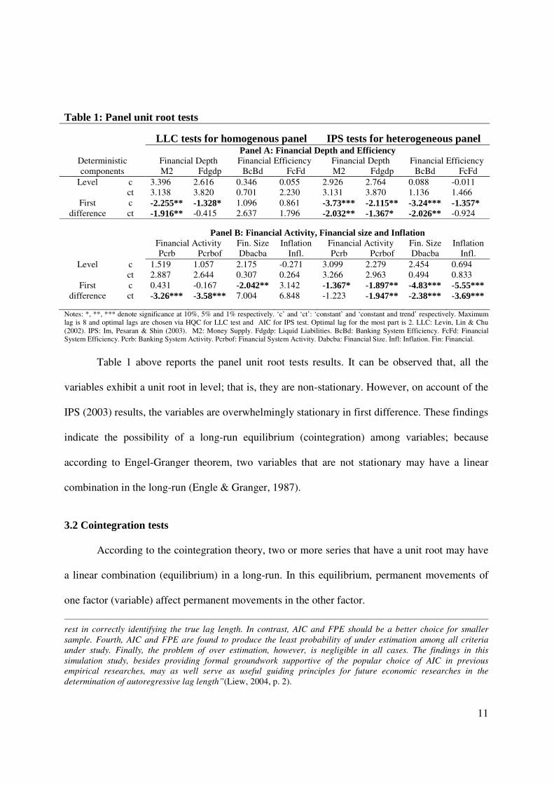
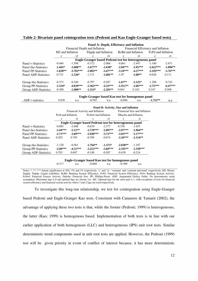
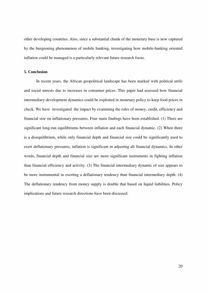
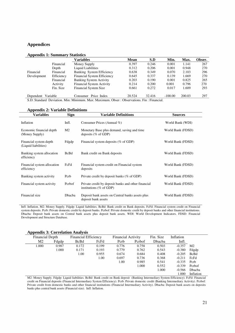
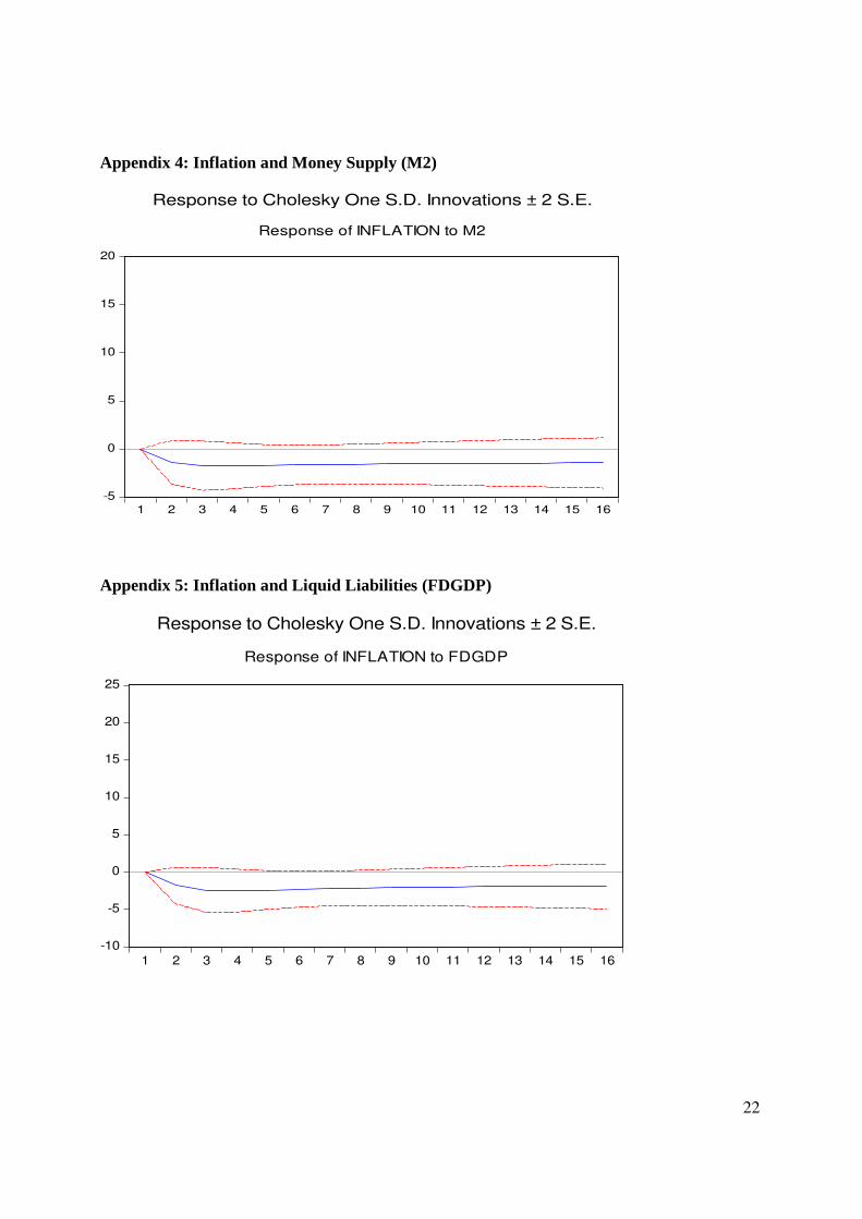
Findings – (1) There are significant long-run equilibriums between inflation and each financial

dynamic. (2) When there is a disequilibrium, while only financial depth and financial size could

be significantly used to exert deflationary pressures, inflation is significant in adjusting all

financial dynamics. In other words, financial depth and financial size are more significant

instruments in fighting inflation than financial efficiency and activity. (3) The financial

intermediary dynamic of size appears to be more instrumental in exerting a deflationary tendency

than financial intermediary depth. (4) The deflationary tendency from money supply is double

that based on liquid liabilities.

Practical implications – Monetary policy aimed at fighting inflation only based on bank

deposits may not be very effective until other informal and semi-formal financial sectors are

taken into account. It could be inferred that, tight monetary policy targeting the ability of banks

to grant credit (in relation to central bank credits) is more effective in tackling consumer price

inflation than that, targeting the ability of banks to receive deposits. In the same vein, adjusting

the lending rate could be more effective than adjusting the deposit rate. The insignificance of

financial allocation efficiency and financial activity as policy tools in the battle against inflation

could be explained by the (well documented) surplus liquidity issues experienced by the African

banking sector.

Social implications – This paper helps in providing monetary policy options in the fight against

soaring consumer prices. By keeping inflationary pressures on food prices in check, sustained

campaigns involving strikes, demonstrations, marches, rallies and political crises that seriously

disrupt economic performance could be mitigated.

Originality/value – As far as we have perused, there is yet no study that assesses monetary

policy options that could be relevant in addressing the dramatic surge in the price of consumer

commodities.

Keywords : Banks; Inflation; Development; Panel; Africa

JEL Classification: E31; G20; O10; O55; P50

3

1. Introduction

During the past decade, the world has seen a dramatic rise in the price of many staple

food commodities. For instance, the price of maize increased by 80% between 2005-2007 and

has since increased further. Many other commodity prices have also soared sharply over this

period: milk powder by 90%, rice by 25% and wheat by 70%. Such large variations in prices

have had tremendous impacts on the incomes of poor households in developing countries (FAO,

2007; World Bank 2008; Ivanic & Martin, 2008). Assessing how to fight inflation is particularly

relevant given its positive incidence on poverty (Fujii, 2011), especially in a continent where

poverty has remained stubbornly high despite financial reforms and structural adjustment

policies (Asongu, 2012a). Also, while low inflation may mitigate inequality (Bulir, 1998; Lopez,

2004), high inflation has been documented to have a negative income redistributive effect

(Albanesi, 2007) in recent African inequality literature (Asongu, 2012a).

The overall effect on poverty rates in African countries is contingent on whether the

gains to poor net producers outweigh the adverse impact on poor consumers. The bearing of food

prices on the situation of particular households also depends importantly on the products

involved, the patterns of households income and expenditure, as well as policy responses of

governments. On account of existing analyses, the impacts of higher food prices on poverty and

inequality are likely to be very diverse; depending on the reasons for the price change and the

structure of the economy (Ravallion & Lokhsin, 2005; Hertel & Winters, 2006). While the

effects of soaring food prices on inequality and poverty may depend on certain circumstances,

most analysts agree that, sustained increased in food prices ultimately leads to sociopolitical

unrests like those experienced in 2008.

4

The World Bank has also raised concerns over the impact of high prices on socio-

political stability (World Bank, 2008). Most studies confirm the link between rising food prices

and the recent waves of revolutions that have marked the geopolitical landscape of developing

countries over the last couple of months (World Bank, 2008; Wodon & Zaman, 2010). The

premises of the Arab Spring and hitherto unanswered questions about some of its dynamics

could be traced to poverty; owing to unemployment and rising food prices. “We will take to the

streets in demonstrations or we will steal,” a 30-year old Egyptian woman in 2008 vented her

anger as she stood outside a bakery. Riots and demonstrations linked to soaring consumer

prices took place in over 30 countries between 2007-08. The Middle East encountered food riots

in Egypt, Jordan, Morocco and Yemen. In Ivory Coast, thousands marched to the home of

President then Laurent Gbagbo chanting: “you are going to kill us”,“ we are hungry”, “life is too

expensive” …etc. Similar demonstrations followed in many other African countries, including ,

Cameroon, Senegal, Ethiopia, Burkina Faso, Mozambique, Mauritania and Guinea. In Latin

America, violent clashes and demonstrations over rising food prices occurred in Guatemala,

Peru, Nicaragua, Bolivia, Argentina, Mexico and the Haitian prime minister was even toppled

following food riots. In Asia, people flooded the streets in Bangladesh, Cambodia, Thailand,

India and the Philippines. Even North Korea surprisingly experienced an incident in which

market women gathered to protest against restrictions on their ability to trade in food (Hendrix et

al., 2009). The geopolitical landscape in the last couple of months has also revolved around the

inability of some political regimes to implement concrete policies that ensure the livelihoods of

their citizens. Tunisia, Egypt, Morocco, Senegal, Uganda, Zambia, Mauritania, Sudan, Western

Sahara and most recently Nigeria are some countries that have witnessed major or minor unrests

5

via techniques of civil resistance in sustained campaigns involving strikes, demonstrations,

marches and rallies.

Whereas the literature on the causes and impacts of the crisis in global food prices in the

developing world has mushroomed in recent years (Piesse & Thirtle, 2009; Wodon & Zaman,

2010; Masters & Shively, 2008), we are unaware of studies that have closely examined how

financial policies affected consumer prices. Remedial policy and pragmatic choices aimed at

fighting inflation that have been documented include both short and medium term responses

(SIFSIA, 2011). Short-term and immediate measures include: input vouchers and input trade

fairs (seeds, fertilizer and tools) for vulnerable farmers; reinforcement of capacity (training and

equipment) in income generating activities; safety-nets (cash transfers or food vouchers); tax

measures and government policies. Medium term measures could be clubbed into three strands:

trade and market measures; production and productivity incentives; coordination and activation

of food security plan. Firstly, trade and market measures include: reduction of import taxes on

basic food items and grain-export bans when needed; strengthening the food and agricultural

market information system; conducting of value chain analysis; building of efficient marketing

institutions; facilitation of farming contract arrangements; lowering of distribution cost; strategic

reserve support and government anticipation of price increase. Secondly, production and

productivity incentives include: investing in agriculture; addressing of poor harvest and

promotion of shelf-life products. Thirdly, coordination and activation of food security action

plan involve: coordination and coherence among various agencies engaged in price stabilization

efforts; comprehensiveness of multi-sectoral responses to price hikes and coordination

(synchronization) of food insecurity plan, in a bid to achieve the maximum impact.

6

According to Von Braun (2008), monetary and exchange rate policy responses were not

effective in addressing food inflation. This revelation by the Director General of the International

Food Policy Research Institute has motivated us to peruse the literature in search of monetary

policies on soaring food prices. Finding none, the present paper fills this gap in the literature by

assessing how financial development dynamics in money, credit, activity, efficiency and size

could be exploited in monetary policy to keep food prices in check. In plainer terms, this work

aims to assess the impact of the following dynamics on food prices. (1) Money: the role of

financial depth (in dynamics of overall economic money supply and financial system liquid

liabilities). (2) Credit: the incidence of financial activity dynamics (in banking and financial

system perspectives). (3) Efficiency: the impact of financial intermediary allocation efficiency

(from banking and financial system angles). (4) Size: the part financial size plays. Another

appeal of this paper is the scarcity of literature on the effect of financial development on inflation

despite a substantial body of work on the economic and financial consequences of inflation

(Barro, 1995; Bruno & Easterly, 1998; Bullard & Keating, 1995; DeGregorio, 1992; Boyd et al.,

2001).

The rest of the paper is organized as follows. Section 2 presents data and discusses the

methodology. Empirical analysis is outlined in Section 3. Discussion and policy implications are

covered in Section 4. Section 5 concludes.

2. Data and Methodology 2.1 Data

We examine a panel of 10 African countries with data from the Financial Development

and Structure Database (FDSD) and African Development Indicators (ADI) of the World Bank

(WB). The ensuing balanced panel is restricted from 1980 to 2010 owing to constraints in data

availability. Information on summary statistics and correlation analysis is detailed in Appendix 1

7

and Appendix 3 respectively. Definition of the variables and corresponding sources are presented

in Appendix 2. Countries in the sample include: Algeria, Egypt, Lesotho, Morocco, Nigeria,

Sudan, Tunisia, Uganda1, Zambia and Tanzania2. The limitation to these countries is primarily

based on the inability of some African countries to exhibit a unit root in consumer price inflation.

Given the problem statement of the study, it is interesting to have non-stationary consumer price

inflation for consistent modeling. Hence, in accordance with recent African law-finance

literature (Asongu, 2011a), CFA franc 3 countries of the CEMAC

4 and UEMOA

5 zones have not

been included6. Beside the justifications for eliminating CFA franc countries provided by

preliminary analysis and recent theoretical postulations (Asongu, 2011a), the seminal work of

Mundell (1972) has shown that, African countries with flexible exchange rates regimes have

more to experience in the fight against inflation than their counterparts with fixed exchange rate

regimes7.

1“Despite decelerating to 27.0 percent in December 2011 from a high of 30.4 percent in October, inflation in

Uganda is still far higher than expected, given the 3 percent rate at the end of 2010. Year-on-year food inflation

spiked to 45.6 percent in October 2011, while non-food inflation has been increasing steadily, moving to 22.8

percent from 5.5 percent in December 2010” (Simpasa et al., 2011, p. 3). 2 “Tanzania inflation reached 19.8 percent in December 2011, well above the 10 percent average for the last few

years. However, in 2010, inflationary pressures started to build, fuelled by soaring food and energy prices, while the

government’s fiscal outlays added to the inflationary pressure. Since October 2010, inflation has more than tripled,

reaching 17.9 percent in October 2011. Although food inflation has slowed recently, it is unlikely to offset other

inflationary pressures ” (Simpasa et al., 2011, p. 3). 3The CFA franc is the name of two currencies used in Africa (by some former French colonies) which are

guaranteed by the French treasury. The two CFA franc currencies are the West African CFA franc (used in the

UEMOA zone) and Central African CFA franc (used in the CEMAC zone). The two currencies though theoretically

separate are effectively interchangeable. 4 Economic and Monetary Community of Central African States.

5 Economic and Monetary Community of West African States.

6 The need for inflation to exhibit a unit root in order to accommodate the problem statement draws from an’

inflation uncertainty’ theory in recent African finance literature. “The dominance of English common–law countries

in prospects for financial development in the legal–origins debate has been debunked by recent findings. Using

exchange rate regimes and economic/monetary integration oriented hypotheses, this paper proposes an 'inflation

uncertainty theory' in providing theoretical justification and empirical validity as to why French civil–law countries

have higher levels of financial allocation efficiency. Inflation uncertainty, typical of floating exchange rate regimes

accounts for the allocation inefficiency of financial intermediary institutions in English common–law countries. As a

policy implication, results support the benefits of fixed exchange rate regimes in financial intermediary allocation

efficiency” Asongu (2011a, p.1). Also, before restricting the dataset, we have found from preliminary analysis that,

African CFA franc countries have a relatively very stable inflation rate. 7 “The French and English traditions in monetary theory and history have been different… The French tradition has

8

In line with the literature (Bordo & Jeanne, 2002; Hendrix et al., 2009) and the problem

statement, the dependent variable is measured in terms of annual percentage change in the

Consumer Price Index (CPI). For clarity in organization, the independent variables are presented

in terms of depth, efficiency, activity and size.

Firstly, from a financial intermediary depth standpoint, we are consistent with the FDSD

and recent African finance literature (Asongu, 2011bcd) in measuring financial depth both from

overall-economic and financial system perspectives with indicators of broad money supply

(M2/GDP) and financial system deposits (Fdgdp) respectively. Whereas the former represents

the monetary base plus demand, saving and time deposits, the latter denotes liquid liabilities of

the financial system. Since we are dealing exclusively with developing countries, we distinguish

liquid liabilities from money supply because a great chunk of the monetary base does not transit

via the banking sector (Asongu, 2011e). The two indicators are in ratios of GDP (see Appendix

2) and can robustly check one another as either account for over 98% of information in the other

(see Appendix 3).

Secondly, by financial efficiency8 here, we neither refer to the profitability-related

concept nor to the production efficiency of decision making units in the financial sector (through

Data Envelopment Analysis: DEA). What the paper aims to elucidate is the ability of banks to

effectively fulfill their fundamental role of transforming mobilized deposits into credit for

stressed the passive nature of monetary policy and the importance of exchange stability with convertibility; stability

has been achieved at the expense of institutional development and monetary experience. The British countries by

opting for monetary independence have sacrificed stability, but gained monetary experience and better developed

monetary institutions.” (Mundell, 1972, pp. 42-43). 8 “It is widely acknowledged that money growth must be seen as more dangerous for price stability when

accompanied by strong credit. On the contrary, robust money growth not associated with sustained credit expansion

and strong dynamics in asset prices seems to be less likely to have inflationary consequences”.(Anonymous

Referee). This is consistent with a recent strand of empirical literature (Bordo & Jeanne, 2002; Borio & Lowe, 2002;

Borio and Lowe, 2004; Detken & Smets, 2004; Van den Noord, 2006; Roffia & Zaghini, 2008; Bhaduri & Durai,

2012). These comment and fact have been incorporated into the analysis from an efficiency standpoint. Financial

intermediary allocation efficiency reflects how money growth (through bank deposits) is accompanied by credit

facilities.

9

economic operators. We adopt indicators of banking-system-efficiency and financial-system-

efficiency (respectively ‘bank credit on bank deposits: Bcbd’ and ‘financial system credit on

financial system deposits: Fcfd’). As with financial depth dynamics, these two financial

allocation efficiency proxies can check each other as either represent more than 95% of

variability in the other (see Appendix 3).

Thirdly, in accordance with the FDSD, we proxy for financial intermediary development

size as the ratio of “deposit bank assets” to “total assets” (deposit bank assets on central bank

assets plus deposit bank assets: Dbacba).

Fourthly, by financial intermediary activity, the paper points out the ability of banks to

grant credit to economic operators. We appreciate both bank-sector-activity and financial-

sector-activity with “private domestic credit by deposit banks: Pcrb” and “private credit by

domestic banks and other financial institutions: Pcrbof” respectively. The former measure

checks the latter as it represents more than 98% of information in the latter (see Appendix 3).

2.2 Methodology

The estimation technique typically follows mainstream literature on fighting inflation

(Bernanke & Gertler, 1995; Detken & Smets, 2004; Goujon, 2006). The estimation approach

entails the following steps: unit root tests, cointegration tests, vector error correction estimation,

Granger causality modeling and impulse-response analysis. Robustness checks are ensured by:

(1) the use of alternative financial indicators; (2) consideration of homogenous and

heterogeneous assumptions in both unit root and cointegration tests; (3) optimal lag selection for

goodness of fit in model specification consistent with the recommendations of Liew (2004); (4)

usage of bivariate analysis to limit causality misspecification issues; (5) application of vector

10

error correction and simple Granger causality and; (6) verifying that, the signs and intervals of

the error correction terms are consistent with theory.

3. Empirical Analysis

3.1 Unit root tests

We begin by testing for serial correlations with two types of panel unit root tests. When

the variables are not stationary in level, we proceed to test for stationarity in first difference.

While short-run Granger causality presupposes the absence of unit roots, the Vector Error

Correction Model (VECM) requires that the variables have a unit root (non stationary) in level

(series). There are two main types of panel unit root tests: first generational (that assumes cross

sectional independence); and second generational (based on cross sectional dependence). A

precondition for the application of the latter is a cross sectional dependence test which is possible

only and only if the number of cross sections (N) in a panel exceed the number of periods in the

cross-sections (T). Hence, we focus on the first generational type. To this end, both the Levin,

Lin & Chu (LLC, 2002) and Im, Pesaran & Shin (IPS, 2003) tests are applied. Whereas the

former is a homogenous based panel unit root test (common unit as null hypothesis), the latter is

a heterogeneous oriented test (individual unit roots as null hypotheses). In case of conflict of

interest in the results, IPS (2003) takes precedence over LLC (2002) in decision making because,

according to Maddala & Wu (1999), the alternative hypothesis of LLC (2002) is too powerful.

Consistent with Liew (2004), goodness of fit is ensured by the Hannan-Quinn Information

Criterion (HQC) and the Akaike Information Criterion (AIC) for the LLC (2002) and IPS (2003)

tests respectively9.

9“The major findings in the current simulation study are previewed as follows. First, these criteria managed to pick

up the correct lag length at least half of the time in small sample. Second, this performance increases substantially

as sample size grows. Third, with relatively large sample (120 or more observations), HQC is found to outdo the

11

Table 1: Panel unit root tests

LLC tests for homogenous panel IPS tests for heterogeneous panel Panel A: Financial Depth and Efficiency

Deterministic

components

Financial Depth Financial Efficiency Financial Depth Financial Efficiency

M2 Fdgdp BcBd FcFd M2 Fdgdp BcBd FcFd

Level c 3.396 2.616 0.346 0.055 2.926 2.764 0.088 -0.011

ct 3.138 3.820 0.701 2.230 3.131 3.870 1.136 1.466

First

difference

c -2.255** -1.328* 1.096 0.861 -3.73*** -2.115** -3.24*** -1.357* ct -1.916** -0.415 2.637 1.796 -2.032** -1.367* -2.026** -0.924

Panel B: Financial Activity, Financial size and Inflation Financial Activity Fin. Size Inflation Financial Activity Fin. Size Inflation

Pcrb Pcrbof Dbacba Infl. Pcrb Pcrbof Dbacba Infl.

Level c 1.519 1.057 2.175 -0.271 3.099 2.279 2.454 0.694

ct 2.887 2.644 0.307 0.264 3.266 2.963 0.494 0.833

First

difference

c 0.431 -0.167 -2.042** 3.142 -1.367* -1.897** -4.83*** -5.55*** ct -3.26*** -3.58*** 7.004 6.848 -1.223 -1.947** -2.38*** -3.69***

Notes: *, **, *** denote significance at 10%, 5% and 1% respectively. ‘c’ and ‘ct’: ‘constant’ and ‘constant and trend’ respectively. Maximum

lag is 8 and optimal lags are chosen via HQC for LLC test and AIC for IPS test. Optimal lag for the most part is 2. LLC: Levin, Lin & Chu

(2002). IPS: Im, Pesaran & Shin (2003). M2: Money Supply. Fdgdp: Liquid Liabilities. BcBd: Banking System Efficiency. FcFd: Financial

System Efficiency. Pcrb: Banking System Activity. Pcrbof: Financial System Activity. Dabcba: Financial Size. Infl: Inflation. Fin: Financial.

Table 1 above reports the panel unit root tests results. It can be observed that, all the

variables exhibit a unit root in level; that is, they are non-stationary. However, on account of the

IPS (2003) results, the variables are overwhelmingly stationary in first difference. These findings

indicate the possibility of a long-run equilibrium (cointegration) among variables; because

according to Engel-Granger theorem, two variables that are not stationary may have a linear

combination in the long-run (Engle & Granger, 1987).

3.2 Cointegration tests

According to the cointegration theory, two or more series that have a unit root may have

a linear combination (equilibrium) in a long-run. In this equilibrium, permanent movements of

one factor (variable) affect permanent movements in the other factor.

rest in correctly identifying the true lag length. In contrast, AIC and FPE should be a better choice for smaller

sample. Fourth, AIC and FPE are found to produce the least probability of under estimation among all criteria

under study. Finally, the problem of over estimation, however, is negligible in all cases. The findings in this

simulation study, besides providing formal groundwork supportive of the popular choice of AIC in previous

empirical researches, may as well serve as useful guiding principles for future economic researches in the

determination of autoregressive lag length”(Liew, 2004, p. 2).

12

Table 2: Bivariate panel cointegration tests (Pedroni and Kao Engle-Granger based tests)

Panel A: Depth, Efficiency and Inflation Financial Depth and Inflation Financial Efficiency and Inflation

M2 and Inflation Fdgdp and Inflation BcBd and Inflation FcFd and Inflation

c ct c ct c ct c ct

Engle-Granger based Pedroni test for heterogeneous panel Panel v-Statistics -0.484 -1.598 -0.712 -2.066 -0.861 -2.447 -1.160 -2.871

Panel rho-Statistics -1.445* -1.686** -1.677** -1.630* -2.84*** -2.95*** -2.622*** -1.896** Panel PP-Statistics -1.828** -3.702*** -2.083** -3.47*** -3.10*** -4.27*** -3.193*** -3.76*** Panel ADF-Statistics -0.721 -1.526* -1.131 -1.681** -1.07 -1.68** -0.626 0.111

Group rho-Statistics -0.373 -0.340 -0.797 -0.287 -1.67** -1.525* -1.208 -0.742

Group PP-Statistics -1.534* -4.029*** -2.362*** -4.33*** -1.911** -2.66*** -2.75*** -6.47*** Group ADF-Statistics -0.300 -1.988** -1.313* -2.291** 0.041 0.183 0.247 0.508

Engle-Granger based Kao test for homogenous panel -ADF t statistics 0.036 n.a -0.592 n.a -0.696 n.a -1.752** n.a

Panel B: Activity, Size and Inflation Financial Activity and Inflation Financial Size and Inflation

Pcrb and Inflation Pcrbof and Inflation Dbacba and Inflation

c ct c ct c ct

Engle-Granger based Pedroni test for heterogeneous panel

Panel v-Statistics -0.885 -2.608 -0.639 -2.377 0.330 -1.653

Panel rho-Statistics -2.44*** -2.12** -2.719*** -2.097** -2.97*** -1.964**

Panel PP-Statistics -2.71*** -3.69*** -2.949*** -3.72*** -3.03*** -3.17***

Panel ADF-Statistics 0.202 0.795 -0.399 -0.074 -3.10*** -2.154**

Group rho-Statistics -1.120 -0.561 -1.764** -1.375* -2.038** -1.187

Group PP-Statistics -2.60*** -4.51*** -3.215*** -5.60*** -2.191** -2.358***

Group ADF-Statistics 0.703 0.697 -0.140 -0.587 -0.439 -0.216

Engle-Granger based Kao test for homogenous panel

-0.317 n.a -0.069 n.a -0.389 n.a

Notes: *, **, *** denote significance at 10%, 5% and 1% respectively. ‘c’ and ‘ct’: ‘constant’ and ‘constant and trend’ respectively. M2: Money

Supply. Fdgdp: Liquid Liabilities. BcBd: Banking System Efficiency. FcFd: Financial System Efficiency. Pcrb: Banking System Activity.

Pcrbof: Financial System Activity. Dabcba: Financial Size. PP: Phillips-Peron. ADF: Augmented Dickey Fuller. No deterministic trend

assumption. Maximum lags is 8 and optimal lags are chosen via AIC. Optimal lags for the most part is 1, with exceptions of tests for financial

system efficiency and financial system activity where 3 and 2 lags are used respectively.

To investigate this long-run relationship, we test for cointegration using Engle-Granger

based Pedroni and Engle-Granger Kao tests. Consistent with Camarero & Tamarit (2002), the

advantage of applying these two tests is that, while the former (Pedroni; 1999) is heterogeneous,

the latter (Kao; 1999) is homogenous based. Implementation of both tests is in line with our

earlier application of both homogenous (LLC) and heterogeneous (IPS) unit root tests. Similar

deterministic trend components used in unit root tests are applied. However, the Pedroni (1999)

test will be given priority in event of conflict of interest because, it has more deterministic

13

components10

. Optimal lag selection for goodness of fit is by the AIC. The choice of bivariate

statistics instead of multivariate statistics is to avoid misspecification in causality estimations11.

Table 2 above reports results of the cointegration tests. While Panel A reports the long-

term relationship between financial depth (efficiency) and inflation, Panel B reveals findings for

the long-run equilibrium between financial activity (size) and inflation. It could be observed

from the Engle-Granger based Pedroni test that, there is overwhelming evidence of a long-term

relationship between each financial dynamic and inflation. It follows that in the long-run,

permanent changes in each financial dynamic affect permanent changes in inflation. Hence, the

need to investigate short-term adjustments to this long-run equilibrium with the VECM.

3.3 Vector Error Correction Model (VECM)

Let us consider inflation and a financial dynamic with no lagged difference, such that:

titi FinanceInflation ,, β= (1)

The resulting VECMs are the following:

ttititi FinanceInflationInflation ,11,1,, )( εβ +−∂=∆ −− (2)

ttititi InflationFinanceFinance ,21,1,, )( εβσ +−=∆ −− (3)

In Eq. (1) and Eq. (2), the right hand terms are the Error Correction Terms (ECTs). At

equilibrium, the value of the ECT is zero. When the ETC is non-zero, it implies that inflation and

a financial dynamic have deviated from the long-run equilibrium; and the ECT helps each

variable to adjust and partially restore the equilibrium. The speeds of these adjustments are

measured by ∂ and σ for inflation and a given financial dynamic respectively. Hence, Eqs. (1)

and (2) are replicated for each ‘financial dynamic and inflation’ pair. The same deterministic

10

Pedroni (1999) is applied in the presence of both ‘constant’ and ‘constant and trend’ while Kao (1999) is based

only on the former (constant). 11

For example, multivariate cointegration may involve variables that are stationary in levels (See Gries et al., 2009).

14

trend assumptions used in the cointegration tests are applied and optimal lag selection for

goodness of fit in model specification is in line with the AIC (Liew, 2004).

Based on results reported in Table 3, while only financial depth and financial size are

exogenous to deflationary pressures, inflation is exogenous to all financial intermediary

dynamics under consideration. In other words, when there is a disequilibrium, while only

financial depth and financial size could be significantly used to exert inflationary pressures,

inflation is significant in adjusting all financial dynamics. Panel A and Panel B are based on Eqs.

(2) and (3) respectively. The ECTs have the expected signs and are in the right interval (See

Section 3.5 on robustness checks for discussion below). In event of a shock, short-run

adjustments of finance to the equilibrium (Panel B) are faster than short-term adjustments of

inflation (Panel A). Hence, finance is more endogenous to inflation than finance is exogenous to

inflation. Since some models (financial efficiency and activity in Panel A for the most part) are

cointegrated with inflation but have no significant corresponding short-term adjustments to long-

run equilibrium, we proceed to analyze the relationship of the variables under consideration by

simple Granger causality.

3.4 Granger Causality

Considering a basic bivariate finite-order VAR model, simple Granger causality is based

on the assessment of how past values of a financial dynamic could help past values of inflation in

explaining the present value of inflation. In mainstream literature, this model is applied on

variables that are not cointegrated (that is, pairs that are stationary in levels). However, within

our framework we are applying this test to all pairs in ‘first difference’ for two reasons: ensure

comparability and; the model can be applied only when variables are stationary and ours are

15

stationary only in ‘first difference’. In light of the above, the resulting VAR models are the

following:

tiijti

q

j

ijjti

p

j

ijti FinanceInflationInflation ,,

0

,

1

, εµδλ ++∆+∆=∆ −=

−=

∑∑ ……..(4)

tiijti

q

j

ijjti

p

j

ijti InflationFinanceFinance ,,

0

,

1

, εµδλ ++∆+∆=∆ −=

−=

∑∑ ………(5)

The null hypothesis of Eq. (4) is the position that, Finance does not Granger cause

Inflation. Hence, a rejection of the null hypothesis is captured by the significant F-statistics;

which is the Wald statistics for the joint hypothesis that estimated parameters of lagged values

equal zero. Optimal lag selection for goodness of fit is in accordance with the AIC (Liew, 2004).

Based on the results reported in Table 3 below, while financial size causes inflation, the latter

causes financial depth (money supply and liquidity liabilities).

Table 3: Vector Error Correction Model and Granger Causality estimations

Panel A: Deflationary Adjustments (Finance effects on Inflation) Financial Depth Fin. Efficiency Financial Activity Fin. Size

M2 Fdgdp BcBd FcFd Pcrb Pcrbof Dbacba

VECM ECT -0.0002*** -0.0001* -0.0001 -0.000 -0.000 -0.000 -0.0006** (t-statistics) (-2.563) (-1.971) (-0.388) (-0.612) (-0.843) (-1.023) (-2.072)

Granger

Causality

Short-run F-stats 1.710 0.816 1.372 2.239 0.625 0.516 3.405**

Panel B: Financial Adjustments (Inflation effects on Finance) Financial Depth Fin. Efficiency Financial Activity Fin. Size

M2 Fdgdp BcBd FcFd Pcrb Pcrbof Dbacba

VECM ECT -0.213*** -0.208*** -0.163*** -0.187*** -0.205*** -0.204*** -0.158** (t-statistics) (-4.945) (-4.865) (-3.811) (-4.736) (-4.781) (-4.851) (-2.344)

Granger

Causality

Short-run F-stats 2.416* 2.510* 0.355 0.442 1.868 1.584 2.228

Notes: *, **, *** denote significance at 10%, 5% and 1% respectively. ‘c’ and ‘ct’: ‘constant’ and ‘constant and trend’ respectively. M2: Money

Supply. Fdgdp: Liquid Liabilities. BcBd: Banking System Efficiency. FcFd: Financial System Efficiency. Pcrb: Banking System Activity.

Pcrbof: Financial System Activity. Dabcba: Financial Size. VECM: Vector Error Correction Model. ECT: Error Correction Term. The

deterministic trend assumptions and lag selection criteria for the VECM are the same as in the cointegration tests (No deterministic trend

assumption. Maximum lag is 8 and optimal lags are chosen via the AIC. Optimal lags for the most part is 1, with exceptions of analyses for

financial system efficiency and financial system activity in which 3 and 2 lags are used respectively). For Granger causality, the optimal lag

selection is based on the AIC. F(t): Fisher (student) statistics. Fin: Financial.

16

3.5 Robustness checks

In order to ensure that our results are robust, we have performed the following. (1) With

the exception of financial size, (for every financial dynamic) two indicators have been employed.

Hence, the findings have encapsulated measures of financial intermediary performance both

from banking and financial system perspectives. (2) Both homogenous and heterogeneous

assumptions are applied in the unit root and cointegration tests. (3) Optimal lag selection for

goodness of fit in model specifications is in line with the recommendations of Liew (2004). (4)

By using bivariate analysis in cointegration tests and corresponding VECM estimations, we have

limited causality misspecification issues. (5) Both VECM and simple Granger VAR

specifications for respectively long-run and short-term causality have been applied. (6) The signs

and intervals of the ECTs conform to theory.

While the first five points have already been elucidated above, the sixth has only been

highlighted. Hence, the need to discuss its relevance to the results. In principle, the speed of

adjustment of the parameters should be between zero and ‘minus one’ (0, -1). If the ECTs are not

within this interval, then either the model is misspecified (and needs adjustment) or the data is

inadequate (perhaps owing to issues with degrees of freedom)12

.

4. Dynamic responses to shocks and policy implications

4. 1 Dynamic responses

Using a Choleski decomposition on a VAR with ordering: 1) inflation, 2) a financial

dynamic; we compute impulse response functions (IRFs) for inflation and financial dynamics.

12

“The error correction term tells us the speed with which our model returns to equilibrium following an exogenous

shock. It should be negatively signed, indicating a move back towards equilibrium, a positive sign indicates

movement away from equilibrium. The coefficient should lie between 0 and 1, 0 suggesting no adjustment one time

period later, 1 indicates full adjustment. The error correction term can be either the difference between the

dependent and explanatory variable (lagged once) or the error term (lagged once), they are in effect the same

thing” (Babazadeh & Farrokhnejad, 2012, p.73).

17

However, given the character of the problem statement in this study, policy implications will be

based on the responses of inflation to shocks in financial dynamics. In other words, how one

standard deviation in financial dynamic innovations affect inflation. A negative response of

inflation to a (positive) shock in a financial dynamic will imply a deflationary tendency in the

consumer price index. Hence, an effective shock in the fight against inflation. Appendices 4-10

present graphical representations corresponding to the IRFs.

The dotted lines shown around the IRFs in Appendices 4-10 are the two standard

deviation bands, which are used as a measure of significance (Agénor et al., 1997, p. 19). A

number of results are noteworthy. Firstly, the results obtained for dynamics of each financial

dimension are broadly similar, indicating robustness of our results to the choice of corresponding

financial dynamics within each financial dimension13. Secondly, shocks in financial dynamics

have a significant impact on the temporary component of inflation. Broadly across the IRFs, a

decrease in a financial intermediary performance dynamic leads to a (temporary) decrease in

inflation (deflation)14

. This effect is consistent with the theoretical predictions and illustrate the

contraction of financial intermediary activities as a measure of fighting inflation. Though all

financial adjustments from a VEC framework are significant with the right signs, from a VAR-

based IRFs framework, (owing to the problem statement), policy implications will only be based

on deflationary adjustments (shocks in financial dynamics of depth and size) because, these have

significant adjustment terms from a VECM-based framework (see Panel A of Table 3).

13

For example, from a financial depth perspective, the response to a money supply shock is similar to that of a liquid

liability shock. In the same vein, the response of a banking efficiency shock is similar to that of a financial

efficiency shock. This same analogy applies to financial intermediary activity (from banking and financial system

perspectives). 14

In Appendix 4, a one standard deviation negative shock to money supply sharply decreases inflation within the

first year, then slightly decreases it again the next year before a slightly steady inflationary effect after the second

year (see response of INFLATION to M2). The deflationary effect in the first year of the shock is consistent with

the liquid liabilities perspective of financial depth in Appendix 5. Here again, a one standard deviation negative

shock of liquidity liabilities has a deflationary pressure on consumer prices within the first year (see response of

INFLATION to FDGDP).

18

Hence, the following findings have been established. (1) There are significant long-run

equilibriums between inflation and each financial dynamic. (2) When there is a disequilibrium,

while only financial depth and financial size could be significantly used to exert deflationary

pressures, inflation is significant in adjusting all financial dynamics. In other words, financial

depth and financial size are more significant instruments in fighting inflation than financial

efficiency and activity. (3) The financial intermediary dynamic of size appears to be more

instrumental in exerting a deflationary tendency than financial intermediary depth. (4) The

deflationary tendency from money supply is double that based on liquid liabilities.

4.2 Policy implications, caveats and future directions

Four main policy implications could be derived from the findings established above.

Firstly, the fact that the effectiveness of money supply as an instrumental tool in fighting

inflation almost doubles that of liquid liabilities (bank deposits) is consistent with theoretical

postulations that, a great chunk of the monetary base in developing countries does not transit

through the banking sector. Hence, monetary policy aimed at fighting inflation only based on

bank deposits may not be very effective until other informal and semi-formal financial sectors

are taken into account. An eloquent example is the growing phenomenon of mobile banking in

African countries (that constitute the monetary base but) not captured by mainstream monetary

policies based on formal financial activities (Asongu, 2012b). Secondly, financial intermediary

size15

appears to be more effective than financial intermediary dynamics of depth (money supply

and bank deposits). In other words, decreasing financial intermediary assets (in relation to central

bank assets) more substantially exerts deflationary pressures on consumer prices. It could

therefore be inferred that, tight monetary policy targeting the ability of banks to grant credit (in

15

Financial size as defined by our paper is also in relative terms (bank assets on total assets). Total assets here refer

to bank assets plus central bank assets. Bank assets refer to credit granted to economic operators.

19

relation to central bank credits) is more effective in fighting consumer price inflation, than that

targeting the ability of banks to receive deposits. In the same vein, adjusting the lending rate

could be more effective than adjusting the deposit rate. Thirdly, we have seen that financial

depth and financial size are more significant instruments in fighting inflation than financial

efficiency16

and activity17

. The deflationary effects of reducing financial allocation efficiency

and credit allocation have had the rights signs but not significant. While inherent surplus

liquidity issues in African banks could explain the insignificance of the efficiency dimension

(Saxegaard, 2006), we expected the inflation-mitigation effect of financial activity to be

significant. The insignificant character of financial activity as an effective instrument in fighting

inflation may be sample-specific. Hence, the result should not be treated with caution and not

generalized to all African countries18.

To the best of our knowledge, the absence of literature dedicated to examining the

bearing of financial dynamics on inflation makes our results less comparable. In this paper, we

have only considered financial intermediary determinants of inflation. But in the real world,

inflation is endogenous to a complex set of variables: exchange rates, wages, price controls…etc.

Thus, the interaction of money, credit, efficiency and size elasticities of inflation with other

determinants of inflation could result in other dynamics of consumer price variations.

Hence, it would be interesting to replicate the analysis in a multivariate VAR context.

Another interesting future research direction could be to assess whether the findings apply to

16

Financial allocation efficiency in the context of this paper refers to the probability of deposits being transformed

into credit for economic operators. In other words, financial intermediation efficiency is the ability of financial depth

to allocate credit for financial activity. Thus financial efficiency is a relative measure (see Beck et al.,1999). 17

Financial activity in the context of this paper refers to the ability of financial institutions to grant credit to

economic operators. 18

The insignificance of financial allocation efficiency and financial activity as policy tools in the battle against

inflation could be explained by the well documented surplus liquidity issues experienced by the African banking

sector (Saxegaard, 2006). Thus, allocation inefficiency (due to low transformation of mobilized funds into credit)

and slow financial activity (limited granting of credit to economic operators) could partly elucidate this finding.

20

other developing countries. Also, since a substantial chunk of the monetary base is now captured

by the burgeoning phenomenon of mobile banking, investigating how mobile-banking oriented

inflation could be managed is a particularly relevant future research focus.

5. Conclusion

In recent years, the African geopolitical landscape has been marked with political strife

and social unrests due to increases in consumer prices. This paper had assessed how financial

intermediary development dynamics could be exploited in monetary policy to keep food prices in

check. We have investigated the impact by examining the roles of money, credit, efficiency and

financial size on inflationary pressures. Four main findings have been established. (1) There are

significant long-run equilibriums between inflation and each financial dynamic. (2) When there

is a disequilibrium, while only financial depth and financial size could be significantly used to

exert deflationary pressures, inflation is significant in adjusting all financial dynamics. In other

words, financial depth and financial size are more significant instruments in fighting inflation

than financial efficiency and activity. (3) The financial intermediary dynamic of size appears to

be more instrumental in exerting a deflationary tendency than financial intermediary depth. (4)

The deflationary tendency from money supply is double that based on liquid liabilities. Policy

implications and future research directions have been discussed.

21

Appendices Appendix 1: Summary Statistics Variables Mean S.D Min. Max. Obser.

Financial

Development

Financial

Depth

Money Supply 0.397 0.246 0.001 1.141 267

Liquid Liabilities 0.312 0.206 0.001 0.948 270

Financial

Efficiency

Banking System Efficiency 0.638 0.349 0.070 2.103 296

Financial System Efficiency 0.645 0.337 0.139 1.669 270

Financial

Activity

Banking System Activity 0.203 0.190 0.001 0.825 265

Financial System Activity 0.214 0.200 0.001 0.796 270

Fin. Size Financial System Size 0.661 0.272 0.017 1.609 293

Dependent Variable Consumer Price Index 20.524 32.416 -100.00 200.03 297

S.D: Standard Deviation. Min: Minimum. Max: Maximum. Obser : Observations. Fin : Financial.

Appendix 2: Variable Definitions

Variables Sign Variable Definitions Sources

Inflation Infl. Consumer Prices (Annual %) World Bank (WDI)

Economic financial depth

(Money Supply)

M2 Monetary Base plus demand, saving and time

deposits (% of GDP)

World Bank (FDSD)

Financial system depth

(Liquid liabilities)

Fdgdp Financial system deposits (% of GDP) World Bank (FDSD)

Banking system allocation

efficiency

BcBd Bank credit on Bank deposits World Bank (FDSD)

Financial system allocation

efficiency

FcFd Financial system credit on Financial system

deposits

World Bank (FDSD)

Banking system activity Pcrb Private credit by deposit banks (% of GDP) World Bank (FDSD)

Financial system activity Pcrbof Private credit by deposit banks and other financial

institutions (% of GDP)

World Bank (FDSD)

Financial size Dbacba Deposit bank assets on Central banks assets plus

deposit bank assets

World Bank (FDSD)

Infl: Inflation. M2: Money Supply. Fdgdp: Liquid liabilities. BcBd: Bank credit on Bank deposits. FcFd: Financial system credit on Financial

system deposits. Pcrb: Private domestic credit by deposit banks. Pcrbof: Private domestic credit by deposit banks and other financial institutions.

Dbacba: Deposit bank assets on Central bank assets plus deposit bank assets. WDI: World Development Indicators. FDSD: Financial

Development and Structure Database.

Appendix 3: Correlation Analysis

Financial Depth Financial Efficiency Financial Activity Fin. Size Inflation M2 Fdgdp BcBd FcFd Pcrb Pcrbof Dbacba Infl.

1.000 0.987 0.172 0.199 0.776 0.758 0.503 -0.357 M2

1.000 0.171 0.193 0.779 0.762 0.543 -0.380 Fdgdp

1.00 0.955 0.674 0.684 0.408 -0.205 BcBd

1.00 0.697 0.736 0.368 -0.211 FcFd

1.00 0.985 0.541 -0.335 Pcrb

1.000 0.552 -0.339 Pcrbof

1.000 -0.566 Dbacba

1.000 Inflation M2: Money Supply. Fdgdp: Liquid liabilities. BcBd: Bank credit on Bank deposit (Banking Intermediary System Efficiency). FcFd: Financial

credit on Financial deposits (Financial Intermediary System Efficiency). Pcrb: Private domestic credit (Banking Intermediary Activity). Pcrbof:

Private credit from domestic banks and other financial institutions (Financial Intermediary Activity). Dbacba: Deposit bank assets on deposits

banks plus central bank assets (Financial size). Infl: Inflation.

22

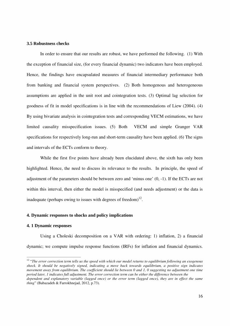
Appendix 4: Inflation and Money Supply (M2)

-5

0

5

10

15

20

1 2 3 4 5 6 7 8 9 10 11 12 13 14 15 16

Response of INFLATION to M2

Response to Cholesky One S.D. Innovations ± 2 S.E.

Appendix 5: Inflation and Liquid Liabilities (FDGDP)

-10

-5

0

5

10

15

20

25

1 2 3 4 5 6 7 8 9 10 11 12 13 14 15 16

Response of INFLATION to FDGDP

Response to Cholesky One S.D. Innovations ± 2 S.E.

23

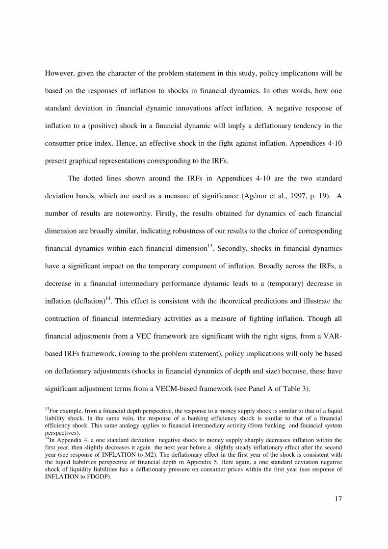
Appendix 6: Inflation and Banking System Efficiency (BCBD)

-10

-5

0

5

10

15

20

25

1 2 3 4 5 6 7 8 9 10 11 12 13 14 15 16

Response of INFLATION to BCBD

Response to Cholesky One S.D. Innovations ± 2 S.E.

Appendix 7: Inflation and Financial System Efficiency (FCFD)

-10

-5

0

5

10

15

20

25

1 2 3 4 5 6 7 8 9 10 11 12 13 14 15 16

Response of INFLATION to FCFD

Response to Cholesky One S.D. Innovations ± 2 S.E.

24

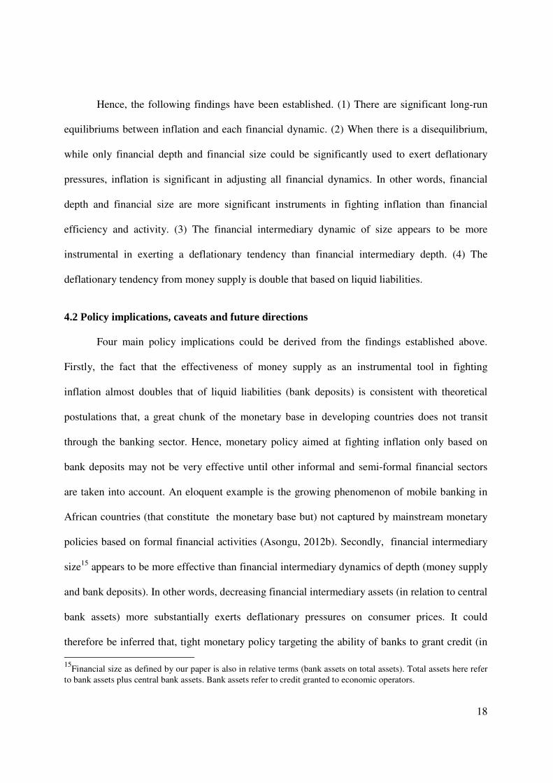
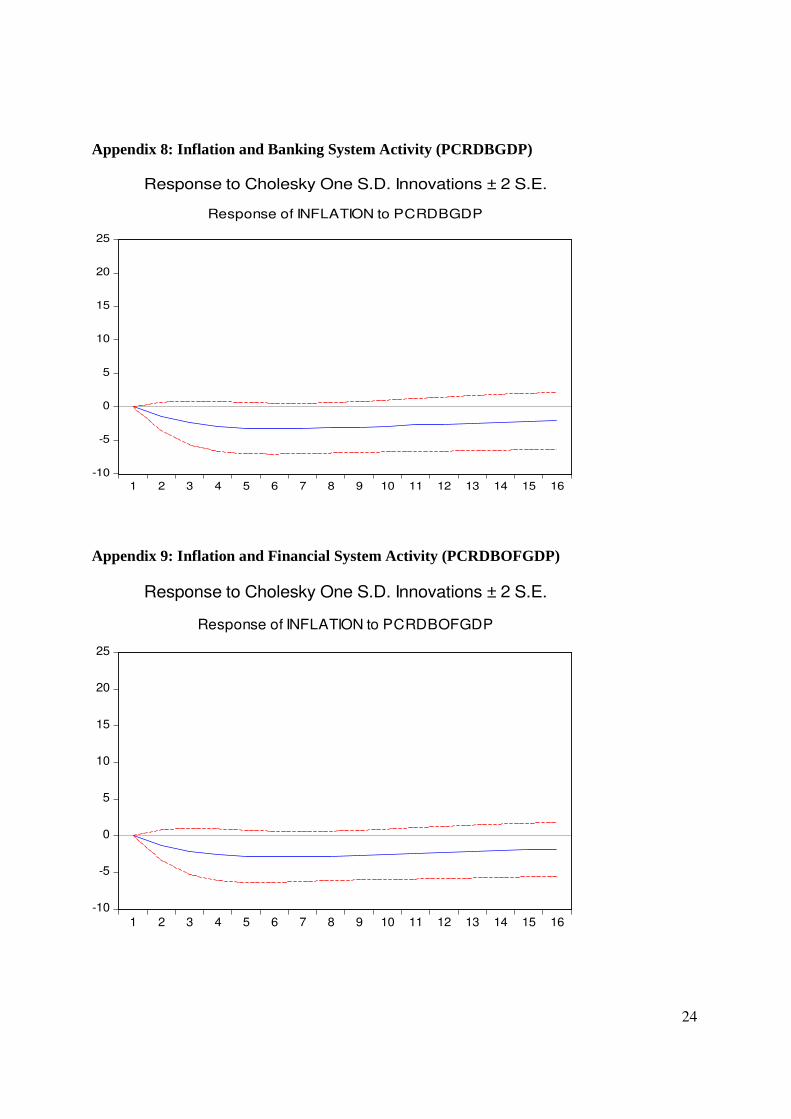
Appendix 8: Inflation and Banking System Activity (PCRDBGDP)

-10

-5

0

5

10

15

20

25

1 2 3 4 5 6 7 8 9 10 11 12 13 14 15 16

Response of INFLATION to PCRDBGDP

Response to Cholesky One S.D. Innovations ± 2 S.E.

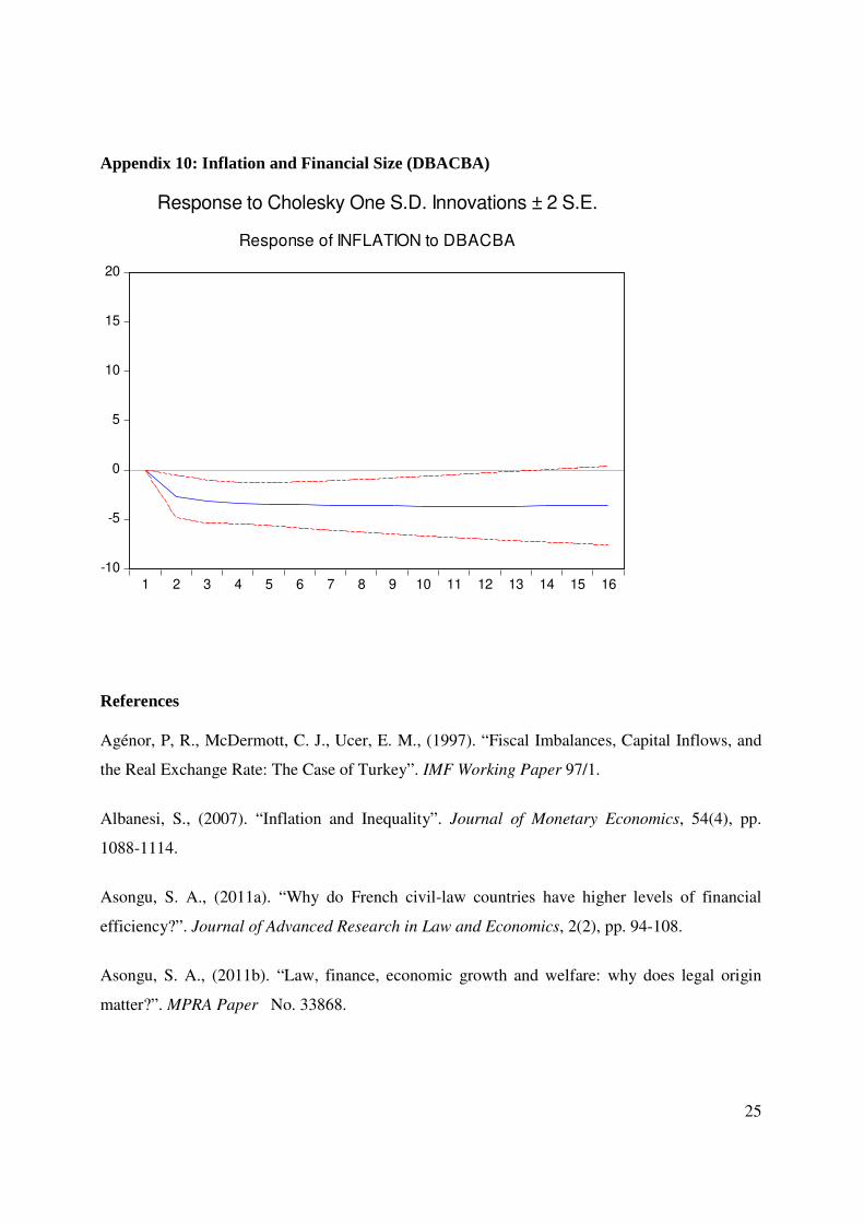
Appendix 9: Inflation and Financial System Activity (PCRDBOFGDP)

-10

-5

0

5

10

15

20

25

1 2 3 4 5 6 7 8 9 10 11 12 13 14 15 16

Response of INFLATION to PCRDBOFGDP

Response to Cholesky One S.D. Innovations ± 2 S.E.

25

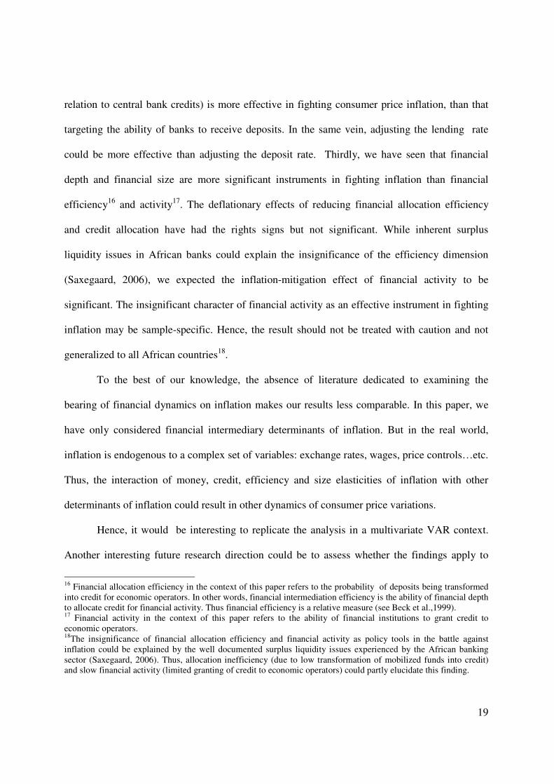
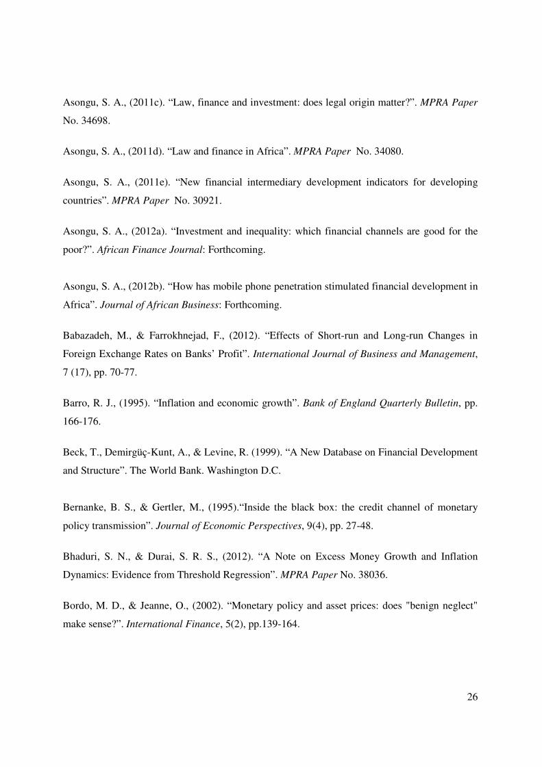
Appendix 10: Inflation and Financial Size (DBACBA)

-10

-5

0

5

10

15

20

1 2 3 4 5 6 7 8 9 10 11 12 13 14 15 16

Response of INFLATION to DBACBA

Response to Cholesky One S.D. Innovations ± 2 S.E.

References

Agénor, P, R., McDermott, C. J., Ucer, E. M., (1997). “Fiscal Imbalances, Capital Inflows, and

the Real Exchange Rate: The Case of Turkey”. IMF Working Paper 97/1.

Albanesi, S., (2007). “Inflation and Inequality”. Journal of Monetary Economics, 54(4), pp.

1088-1114.

Asongu, S. A., (2011a). “Why do French civil-law countries have higher levels of financial

efficiency?”. Journal of Advanced Research in Law and Economics, 2(2), pp. 94-108.

Asongu, S. A., (2011b). “Law, finance, economic growth and welfare: why does legal origin

matter?”. MPRA Paper No. 33868.

26

Asongu, S. A., (2011c). “Law, finance and investment: does legal origin matter?”. MPRA Paper

No. 34698.

Asongu, S. A., (2011d). “Law and finance in Africa”. MPRA Paper No. 34080.

Asongu, S. A., (2011e). “New financial intermediary development indicators for developing

countries”. MPRA Paper No. 30921.

Asongu, S. A., (2012a). “Investment and inequality: which financial channels are good for the

poor?”. African Finance Journal: Forthcoming.

Asongu, S. A., (2012b). “How has mobile phone penetration stimulated financial development in

Africa”. Journal of African Business: Forthcoming.

Babazadeh, M., & Farrokhnejad, F., (2012). “Effects of Short-run and Long-run Changes in

Foreign Exchange Rates on Banks’ Profit”. International Journal of Business and Management,

7 (17), pp. 70-77.

Barro, R. J., (1995). “Inflation and economic growth”. Bank of England Quarterly Bulletin, pp.

166-176.

Beck, T., Demirgüç-Kunt, A., & Levine, R. (1999). “A New Database on Financial Development

and Structure”. The World Bank. Washington D.C.

Bernanke, B. S., & Gertler, M., (1995).“Inside the black box: the credit channel of monetary

policy transmission”. Journal of Economic Perspectives, 9(4), pp. 27-48.

Bhaduri, S. N., & Durai, S. R. S., (2012). “A Note on Excess Money Growth and Inflation

Dynamics: Evidence from Threshold Regression”. MPRA Paper No. 38036.

Bordo, M. D., & Jeanne, O., (2002). “Monetary policy and asset prices: does "benign neglect"

make sense?”. International Finance, 5(2), pp.139-164.

27

Borio, C., & Lowe, P., (2002). “Asset prices, financial and monetary stability: exploring the

nexus”. BIS Working Paper No.114.

Borio, C., & Lowe, P., (2004). “Securing sustainable price stability: should credit come back

from the wilderness?”. BIS Working Paper No.157.

Boyd, J. H., Levine, R., & Smith, B. D., (2001). “The impact of inflation on financial sector

performance”. Journal of Monetary Economics, 47, pp. 221-248.

Bruno, M., & Easterly, W., (1998). “Inflation crises and long-run growth”. Journal of Monetary

Economics, 41, pp. 3-26.

Bulir, A., (1998). “Income inequality: does inflation matter?”. IMF Working Paper No. 98/7.

Bullard, J., & Keating, J., (1995). “The long-run relationship between inflation and output in

postwar economies”. Journal of Monetary Economics, 36, pp. 477-496.

Camarero, M., & Tamarit, C., (2002). “A panel cointegration approach to the estimation of the

peseta real exchange rate”. Journal of Macroeconomics. 24, pp. 371-393.

DeGregorio, J., (1992). “The effects of inflation on economic growth”, European Economic

Review, 36(2-3), pp. 417-424.

Detken, C., & Smets, F., (2004). “Asset price booms and monetary policy”, in Horst Siebert (ed.)

Macroeconomic Policies in the World Economy, Springer, Berlin, pp. 189-227.

Engle, R. F., & Granger, W. J., (1987). “Cointegration and error correction: Representation,

estimation and testing”. Econometrica, 55, pp. 251-276.

Fujii, T., (2011). “Impact of food inflation poverty in the Philippines”. SMU Economics &

Statistics Working Paper No. 14-2011.

28

Goujon, M., (2006). “Fighting inflation in a dollarized economy: The case of Vietnam”. Journal

of Comparative Economics, 34, pp. 564-581.

Gries, T., Kraft, M., & Meierrieks, D., (2009). “Linkages between financial deepening, trade

openness, and economic development: causality evidence from Sub-Saharan Africa”. World

Development, 37(12), pp. 1849-1860.

FAO. (2007). Food Outlook, November. http://www.fao.org/docrep/010/ah876e/ah876e00.htm

(accessed on: 7/10/2012).

Hendrix, C., Haggard, S., & Magaloni, B., (2009). “Grievance and Opportunity : Food Prices ,

Political Regime and Protest”, Paper prepared for presentation at the International Studies

Association Convention, New York (August, 2009).

Hertel, T. W., & Winters, L. A., (2006). Poverty and the WTO: Impacts of the Doha

Development Agenda. Basingstoke and Washington DC: Palgrave-Macmillan and the

World Bank (L. A. eds).

Im, K. S., Pesaran, M. H., & Shin, Y., (2003). “Testing for unit roots in heterogeneous panels”.

Journal of Econometrics, 115, pp. 53-74.

Ivanic, M., & Martin, W. (2008, April). “Implications of Higher Global Food Prices for Poverty

in Low-Income Countries”, Policy Research Working Paper No. 4594.

Kao, C., (1999). “Spurious regression and residual-based tests for cointegration in panel data”.

Journal of Econometrics, 90, pp. 1–44.

Liew, V. K., (2004). “Which lag selection criteria should we employ?”. Economics Bulletin,

3(33), pp. 1-9.

Levin, A., Lin, C. F., & Chu, C. S., (2002). “Unit root tests in panel data: asymptotic and

29

finite-sample properties”. Journal of Econometrics, 108, pp. 1-24.

Lopéz, J. H., (2004). “Pro-growth, Pro-poor: Is There a Tradeoff?”. World Bank Publications.

Maddala, G. S., & Wu, S., (1999). “A comparative study of unit root tests with panel data and a

new simple test”. Oxford Bulletin of Economics and Statistics, 61, pp. 631-52.

Masters, W., & Shively, G., (2008). “Special Issue on the World Food Crisis”, Agricultural

Economics, 39, pp. 373-374.

Mundell, R., (1972). African trade, politics and money. In Tremblay, R., ed., Africa and

Monetary Integration. Les Editions HRW, Montreal, pp. 11-67.

Pedroni, P., (1999). “Critical values for cointegration tests in heterogeneous panels with

multiple regressors”. Oxford Bulletin of Economics and Statistics, Special Issue .pp. 653-670.

Piesse, J., & Thirtle, C., (2009). “Three bubbles and a panic: an explanatory review of recent

food commodity price events”. Food Policy, 34(2), pp. 119-129.

Ravallion, M., & Lokshin, M., (2005). “Winners and Losers from Trade Reform in Morocco”

Mimeo, World Bank.

Roffia, B., & Zaghini, A., (2008). “Excess Money Growth and Inflation Dynamics”, Bank of

Italy Temi di Discussione, Working Paper No. 657.

Saxegaard, M., (2006). “Excess liquidity and effectiveness of monetary policy: evidence from

sub-Saharan Africa”, IMF Working Paper 06/115.

SIFSIA (2011). “Soaring food prices and its policy implications in North Sudan: a policy brief”,

Sudan Institutional Capacity Programme: Food Security Information Action, pp. 1-14.

30

Simpasa, A., Gurara, D., Shimeles, A., Vencatachellum, D., Ncube, M., (2011). “Inflation

Dynamics in selected East African countries: Ethiopia, Kenya, Tanzania and Uganda”, AfDB

Policy Brief.

Van den Noord, P., (2006). “Are house price near a peak? A probit analysis for 17 OECD

countries”, OECD Economic Department Working Paper No.488.

Von Braun, J., (2008). “Rising Food Prices: Dimension, Causes, Impact and Responses”. Key

Note Address at World Food Programme (9th April 2008).

<http://documents.wfp.org/stellent/groups/public/documents/resources/wfp175955.pdf>

(accessed: 21.01.12).

Wodon, Q., & Zaman, H., (2010). “High food prices in sub-Saharan Africa: poverty impact and

policy responses”. World Bank Research Observer, 25(1), pp. 157-176.

World Bank (2008). High food prices: a harsh new reality.

http://econ.worldbank.org/WBSITE/EXTERNAL/EXTDEC/0,,contentMDK:2166588

3~pagePK:64165401~piPK:64165026~theSitePK:469372,00.html (accessed: 21.01.12).


Recommended