121
Final Contaminant Candidate List 3 Chemicals: Classification of the PCCL to CCL

Final Contaminant Candidate List 3 Chemicals: Classification of the PCCL to CCL

Office of Water (4607M) EPA 815-R-09-008 August 2009 www.epa.gov/safewater

i of vi
EPA-OGWDW Final CCL 3 Chemicals: EPA 815-R-09-008 Classification of the PCCL to CCL August 2009
Table of Contents 1.0 INTRODUCTION TO THE CONTAMINANT CANDIDATE LIST (CCL)
CLASSIFICATION PROCESS ........................................................................................1
1.1 Principles of Evaluation .................................................................................................... 2 1.2 Developing the Classification Approach .......................................................................... 3
2.0 ATTRIBUTES .........................................................................................................................5
2.1 Health Effects Attributes ................................................................................................... 6 2.1.1 Potency .......................................................................................................................... 6 2.1.2 Severity ....................................................................................................................... 15
2.2 Occurrence Attributes ..................................................................................................... 20 2.2.1 Prevalence and Magnitude Data Elements.................................................................. 21 2.2.2 Prevalence - Calibrating Scales and Scoring .............................................................. 22 2.2.3 Evaluation of the Prevalence Protocol ........................................................................ 23 2.2.4 Magnitude - Calibrating Scales and Scoring .............................................................. 24 2.2.5 Persistence-Mobility as a Surrogate Measure for Magnitude ..................................... 29 2.2.6 Persistence-Mobility Data – Calibrating Scales and Scoring ..................................... 30 2.2.7 Evaluation of the Magnitude Protocol ........................................................................ 31
2.3 Fine Tuning the Protocols ............................................................................................... 32 3.0 DEFINITIONS AND OVERVIEW OF THE TRAINING DATA SET ..........................32
3.1 Key Considerations .......................................................................................................... 33 3.2 Developing Key Components of the Training Data Set ................................................ 33
3.2.1 Attribute Scores .......................................................................................................... 33 3.2.2 Making L ist-Not list Decisions ................................................................................... 37
4.0 PROTOTYPE CLASSIFICATION MODELS AND THE CCL PROCESS ..................38
4.1 Model Training and Development.................................................................................. 39 4.2 Model Sensitivity Analyses .............................................................................................. 41
4.2.1 Training w ith subsets of the TDS ............................................................................... 41 4.2.2 Training a fter Selected “Outliers” Are Removed From the TDS ............................... 42 4.2.3 Graphical and Statistical Analyses to Identify Significant Differences in
Attribute “Weights” Or Influence on Model Performance ....................................... 43 4.3 Model Performance Testing ............................................................................................ 45 4.4 Evaluating Classification Differences ............................................................................ 46
4.4.1 Classification Differences Among the Models ........................................................... 47 4.4.2 Logical Evaluation of the Models – Graphical Analysis ............................................ 49
4.5 Applying Model Results .................................................................................................. 55 4.5 Applying Model Results .................................................................................................. 56
4.5.1 Additive Model Results .............................................................................................. 56 4.5.2 Additive Rank Order Results ...................................................................................... 56

EPA-OGWDW Final CCL 3 Chemicals: EPA 815-R-09-008 Classification of the PCCL to CCL August 2009
5.0 MODEL OUTCOME AND POST MODEL EVALUATION PROCESS ......................58
5.1 PCCL Characterization and Model Results .................................................................. 58 5.2 Evaluation of the Modeling Output ............................................................................... 59
5.2.1 Procedure .................................................................................................................... 59 5.2.2 Evaluation Results ...................................................................................................... 60
5.3 Post-Model Adjustments to Output ............................................................................... 62 5.3.1 Using Supplemental Sources to Identify the Data Most Relevant to Drinking
Water ......................................................................................................................... 63 5.3.2 Calculation of a Health-Concentration Ratio for Contaminants with Water
Data ........................................................................................................................... 63 5.3.3 Grouping Contaminants based on Data Certainty ...................................................... 66 5.3.4 LD50 Values with Limited Documentation ................................................................. 67
5.4 Selecting the Draft CCL 3 ............................................................................................... 67 5.5 Summary ........................................................................................................................... 68
6.0 REFERENCES ......................................................................................................................69
7.0 APPENDICES .......................................................................................................................70
Appendix A. Attribute Scoring Protocols ........................................................................... A-1 Appendix B. Information Sheets from the TDS Exercises .................................................B-1 Appendix C. Summary of EPA Team TDS Decisions ....................................................... C-1 Appendix D. Software Sources ............................................................................................ D-1 Appendix E. Solutions ...........................................................................................................E-1 Appendix F. Chemicals Reviewed by the EPA Evaluation Team: Summary of
Results ......................................................................................................................... F-1 Appendix G. PCCL Contaminants with Incomplete Data for Scoring or that had
Parent Compounds Scored in Developing the Draft CCL 3 ................................. G-1
ii of vi

EPA-OGWDW Final CCL 3 Chemicals: EPA 815-R-09-008 Classification of the PCCL to CCL August 2009
Table of Exhibits Exhibit 1. Developing an Approach to Process PCCL Chemicals ................................................. 4
Exhibit 2. Decile Distribution of RfD Values (mg/kg/day) ............................................................ 8
Exhibit 3A. Logarithmic Distribution of RfD Values .................................................................... 9
Exhibit 3B. Logarithmic Distribution of NOAEL Values ............................................................. 9
Exhibit 3C. Logarithmic Distribution of LOAEL Values ............................................................ 10
Exhibit 3D. Logarithmic Distribution of LD50 Values ................................................................. 10
Exhibit 4. Scoring Equations for Potency ..................................................................................... 12
Exhibit 5. Logarithmic Distribution of Cancer Potency Values ................................................... 13
Exhibit 6. Potency Scores for Chemicals in the Learning Set ...................................................... 14
Exhibit 7. Potency Scores for Chemicals Not in the Learning Set ............................................... 14
Exhibit 8. NRC Severity Scoring Proposal ................................................................................... 16
Exhibit 9. Final Nine-Point Scoring Protocol for Severity ........................................................... 17
Exhibit 10. Relationship of Data Elements Used to Score Magnitude and Prevalence. ............... 21
Exhibit 11. Comparison of Prevalence Scores for Learning Set Contaminants ........................... 23
Exhibit 12. Comparison of the NRC Magnitude Score with the Ratio of the Health Advisory Guideline to the Concentration in Finished Water ....................................... 25
Exhibit 13. Magnitude Concentrations and Scores Derived from Potency Doses ....................... 26
Exhibit 14A. Equal Bins Drinking Water Magnitude Scale (ug/L) .............................................. 27
Exhibit 14B. Half Log Option A Drinking Water Magnitude Scale (ug/L) ................................. 27
Exhibit 14C. Half Log Option B Drinking Water Magnitude Scale (ug/L) ................................. 28
Exhibit 15. Magnitude Attribute Scores: Example Contaminants Scored by their Median of Detections Using the Various Approaches in Exhibit 14. ....................................... 28
Exhibit 16. Mobility and Persistence Data Elements.................................................................... 29
Exhibit 17. Comparison of Scores derived using the Magnitude Protocol ................................... 31
Exhibit 18. Combinations of low and high attribute scores1 for the four attributes using Latin Hypercube Sampling. ......................................................................................... 35
Exhibit 19. Attribute Space for the 101 TDS compared to that for the 202 TDS ......................... 36
Exhibit 20a. QUEST Classifications Based on the Full Training Data Set .................................. 40
Exhibit 20b. QUEST Classifications Based on 5-Fold Cross-Validation..................................... 40
Exhibit 21. Linear Model-estimated versus Team Average Classification for the TDS ............. 43
Exhibit 22. Relative Weights of Attributes at QUEST Nodes ...................................................... 44
Exhibit 23. Summary Statistics from MCMC Sample.................................................................. 45
iii of vi

EPA-OGWDW Final CCL 3 Chemicals: EPA 815-R-09-008 Classification of the PCCL to CCL August 2009
Exhibit 24. Features of the Three Preferred Models Based on TDS Test Results ........................ 46
Exhibit 25. Decision Comparison Matrix; Weight of Differences ............................................... 47
Exhibit 26. Summary of Quaternary Model Decisions ................................................................. 48
Exhibit 27. Results of 202 Model Classifications and Weighted Misclassifications ................... 48
Exhibit 28. Summary of Individual Quaternary Model Classifications ....................................... 50
Exhibit 29. ANN Model Predictions for the Four Attribute Space............................................... 51
Exhibit 30. MARS Model Predictions for the Four Attribute Space ............................................ 53
Exhibit 31. Univariate CART Model Predictions for the Four Attribute Space ........................... 54
Exhibit 32. Linear Model Predictions for the Four Attribute Space ............................................. 54
Exhibit 32. Linear Model Predictions for the Four Attribute Space ............................................. 55
Exhibit 33. Summary Comparison of the Sum of the 3 Model Decisions to the Distribution of EPA Blinded (TDS) Decisions ............................................................ 57
Exhibit 34. Model Results for the PCCL Chemicals .................................................................... 58
Exhibit 35. Results of the Model Output Evaluation (Total = 129 chemicals)............................. 62
Exhibit 36. Formulae used in the CCL 3 Process to Calculate Health Reference Levels (HRLs) from the CCL 3 Potency Data Elements. ........................................................ 64
iv of vi

EPA-OGWDW Final CCL 3 Chemicals: EPA 815-R-09-008
Classification of the PCCL to CCL August 2009
v of vi
List of Abbreviations and Acronyms < Less than < Less than or equal to > Greater than > Greater than or equal to µg Microgram, one-millionth of a gram µg/L Micrograms per liter ANN Artificial Neural Network ATSDR Agency for Toxic Substances and Disease Registry CART Classification and Regression Tree CASRN Chemical abstract services registry number CCL Contaminant Candidate List CCL 1 EPA’s first contaminant candidate list CCL 2 EPA’s second Contaminant Candidate List CCL 3 EPA’s third Contaminant Candidate List CUS/IUR Chemical update system/inventory update rule DBP Disinfection byproduct EDWC Estimated Drinking Water Concentration EEC Estimated Environmental Concentration EPA United States Environmental Protection Agency g/day Grams per day HRL Health Reference Level IOC Inorganic compound IRIS Integrated Risk Information System kg Kilogram L Liter LD50 Lethal dose 50; an estimate of a single dose that is expected to cause the death
of 50 percent of the exposed animals; it is derived from experimental data. lbs Pounds LOAEL Lowest observed adverse effect level MARS Multivariate Adaptive Regression Splines MCMC Markov Chain Monte Carlo mg Milligram, one-thousandth of a gram mg/kg Milligrams per kilogram body weight

EPA-OGWDW Final CCL 3 Chemicals: EPA 815-R-09-008
Classification of the PCCL to CCL August 2009
vi of vi
mg/kg/day Milligrams per kilogram body weight per day mg/L Milligrams per liter N Number of samples NAWQA National water quality assessment (USGS program) NCOD National contaminant occurrence database ND Not detected (or non-detect) NDWAC National Drinking Water Advisory Council NIRS National Inorganic and Radionuclide Survey NOAEL No observed adverse effect level NRC National Research Council OW Office of Water OPP Office of Pesticide Programs PBPK Physiologically Based Pharmacokinetic PCCL Preliminary-CCL PWS Public water system QUEST Quick, Unbiased, Efficient Statistical Tree RTECs Registry of Toxic Effects of Chemical Substances RfD Reference dose TDS Training data set TRI Toxics Release Inventory UCMR Unregulated Contaminant Monitoring Regulations UCMR 1 First Unregulated Contaminant Monitoring Regulation UCMR 2 Second Unregulated Contaminant Monitoring Regulation UL Tolerable upper intake level US United States of America USGS United States Geological Survey

EPA-OGWDW Final CCL 3 Chemicals: EPA 815-R-09-008
Classification of the PCCL to CCL August 2009
Page 1 of 70
1.0 INTRODUCTION TO THE CONTAMINANT CANDIDATE LIST (CCL) CLASSIFICATION PROCESS Every five years the United States Environmental Protection Agency (EPA) is required to publish a list of contaminants (1) that are currently unregulated, (2) that are known or anticipated to occur in public water systems, and (3) which may require regulations under the Safe Drinking Water Act (SDWA). This list is known as the Contaminant Candidate List or CCL. SDWA section 1412(b)(1) requires that in the development of the CCL, EPA consider specific data sources and include the scientific community. EPA must evaluate substances identified in section 101(14) of the Comprehensive Environmental Response, Compensation, and Liability Act (CERCLA) of 1980 and substances registered as pesticides under the Federal Insecticide, Fungicide, and Rodenticide Act (FIFRA). SDWA also requires the Agency to consider the National Contaminant Occurrence Database established under section 1445(g) of SDWA. SDWA directs the Agency to consult with the scientific community, including the Science Advisory Board (SAB). In addition, it directs the Agency to consider the health effects and occurrence information for unregulated contaminants to identify those contaminants that present the greatest public health concern related to exposure from drinking water. EPA interprets the criterion that contaminants are known or anticipated to occur in public water systems broadly. In evaluating this criterion, EPA considers not only public water system monitoring data, but also data on concentrations in ambient surface and ground waters, releases to the environment (e.g., Toxics Release Inventory), and production. While such data may not establish conclusively that contaminants are known to occur in public water systems, EPA believes these data are sufficient to anticipate that contaminants may occur in public water systems and support their inclusion on the CCL. The Agency considered adverse health effects that may pose a greater risk to life stages and other sensitive groups which represent a meaningful portion of the population. Adverse health effects associated with infants, children, pregnant women, the elderly, and individuals with a history of serious illness were evaluated. In selecting contaminants for the CCL 3, each of the above requirements was met. SDWA section 1412(b)(1) also requires EPA to determine whether to regulate at least five contaminants from the CCL every five years. SDWA specifies that EPA shall regulate a contaminant if the Administrator determines that:
• The contaminant may have an adverse effect on the health of persons; • The contaminant is known to occur, or there is a substantial likelihood that the
contaminant will occur in public water systems with a frequency and at levels of public health concern; and
• In the sole judgment of the Administrator, regulation of such contaminant presents a meaningful opportunity for health risk reduction for persons served by public water systems.
Once contaminants have been placed on the CCL, EPA identifies if there are any additional data needs or if there are sufficient information to make a regulatory determination. EPA interprets these criteria for regulatory determination as more rigorous than what is used to place contaminants on the CCL.
EPA-OGWDW Final CCL 3 Chemicals: EPA 815-R-09-008
Classification of the PCCL to CCL August 2009
Page 2 of 70
EPA developed a multi-step approach to select contaminants for the third CCL (CCL 3), which includes the following key steps:
(1) The identification of a broad universe of potential drinking water contaminants (CCL 3 Universe);
(2) A screening process that uses straightforward screening criteria, based on a
contaminant’s potential to occur in public water systems and thereby pose a potential public health concern, to narrow the universe of contaminants to a Preliminary-CCL (PCCL); and
(3) A structured classification process (e.g., a prototype classification algorithm
model) that objectively compares data and information as a tool and is evaluated along with expert judgment to develop a CCL from the PCCL.
Steps 1 and 2 in the process are described in other support documents: Final CCL 3 Chemicals: Identifying the Universe (EPA, 2009a); and Final CCL 3 C hemicals: Screening to a PCCL (EPA, 2009b). The purpose of this document is to describe the methodology used to develop the classification process (Step 3) and the process used to select chemicals for the CCL 3. The PCCL consisted of 561 chemicals that were screened from the CCL3 Universe. To select contaminants for the CCL 3, EPA used classification models to handle larger, more complex assortments of data in a consistent and reproducible manner. Learning from EPA’s experience and expertise, the classification models were trained based on past expert decisions. The algorithms were used to prioritize chemicals which allowed the final expert evaluation and review to be more objective and efficient. The data and information used to evaluate contaminants on the PCCL is provided in Contaminant Information Sheets available in the CCL 3 doc ket (EPA-HQ-OW-2007-1189) at www.regulations.gov. 1.1 Principles of Evaluation In developing the first CCL (CCL 1), the Agency utilized readily available occurrence and health effects information coupled with an expert review process. Following the publication of CCL 1, the Agency sought the advice of the National Research Council (NRC) and National Drinking Water Advisory Council (NDWAC). The panels provided recommendations to guide EPA in creating a more comprehensive and transparent evaluation of potential drinking water contaminants for developing future CCLs. In the light of the NRC and NDWAC recommendations, EPA has reviewed and evaluated a large number of contaminants and their data, developed decision making protocols using classification algorithm approaches, and included expert review in arriving at decisions to list or not list contaminants on CCL 3. These steps have provided a decision process that is more transparent and reproducible than approaches used for previous CCLs. The process is driven by the data on i ndividual contaminants and minimizes the bias that may occur with expert panels related to the participants’ individual backgrounds and the effects of group dynamics. As experience is gained, the new classification process is likely to evolve and improve for application to future CCLs.

EPA-OGWDW Final CCL 3 Chemicals: EPA 815-R-09-008
Classification of the PCCL to CCL August 2009
Page 3 of 70
To guide the development of the classification process, EPA identified several key features that the approach addresses.
1. Meaningful Basis for Classification. The classification process must reflect the critical
goals of the CCL; that is, it must consider the potential for occurrence in water, the potential for causing adverse health effects, and it must prioritize contaminants based on these criteria. The data supporting the list no-list decision must be linked back to these three tenets.
2. Incorporating Relevant Data. The most relevant data used for the classification process
include health effects data that are appropriate for drinking water exposures, and occurrence data that indicate the nature and spatial extent of potential occurrence in drinking water.
3. Transparent Process for Communication. One goal of the classification approach is to
provide a transparent process that can be reviewed by external experts and the public. The attributes and data characterizing the contaminants should be easy to understand and the decision-making process to list or not list a particular contaminant must be conveyed in a straight forward manner.
4. Reproducibility. A key feature of the classification process is that it should be
reproducible. The classification process should always give the same result for the same set of input information.
1.2 Developing the Classification Approach Based on this framework, EPA developed an approach for classifying potential drinking water contaminants. An overarching premise in using classification models to prioritize contaminants is that different contaminants can be compared on the basis of similar attributes. The approach ensures that the contaminant attributes reflect the key decision characteristics in deciding whether or not to list a contaminant on the CCL. The attributes are properties used to categorize contaminants for their potential to occur in drinking water and for their potential to cause adverse health effects. For example, occurrence can be characterized by a contaminant’s water concentration data or potential to occur based on its release to the environment. The adverse health effects of contaminants can be characterized using preliminary toxicological data such as median lethal dose (LD50) or more developed values such as oral reference doses (RfDs). To evaluate, categorize, and prioritize the PCCL contaminants as potential CCL contaminants, EPA integrated various types of data that represent measures of their attributes. This relative assessment across data measures normalized the available data by developing a set of attribute scales for the attribute data, and scoring mechanisms for the various types of data available for potential drinking water contaminants. Because of this new approach and its new application, EPA developed, tested, and evaluated the results of several classification algorithms to assess whether they are useful, and which ones might provide the best decision support tools. To test and evaluate the process, EPA developed a data set and used it to “train” the classification algorithms. Once the modeling was completed, EPA evaluated the model output based on the compilation of data for a subset of the modeled

EPA-OGWDW Final CCL 3 Chemicals: EPA 815-R-09-008
Classification of the PCCL to CCL August 2009
Page 4 of 70
contaminants and assisted in developing a process to utilize the model output to generate the CCL 3. The following chapters describe the steps EPA used to develop the components of the classification process, as displayed in Exhibit 1.
Exhibit 1. Developing an Approach to Process PCCL Chemicals
Develop Attribute Scoring Protocol
Select Training Data Set Contaminants and Make
Listing Decisions
Score Training Data Set Contaminants with Final Attribute
Scoring Protocols
Train and Validate Classification Approaches using Training Data Set
Iterative Process – The results of training and validation will indicate if areas need further evaluation and refinement. The iterative process may or may not go back to the primary assumptions.
Adequate Results
Apply to PCCL
Post-model evaluation of PCCL
chemicals
Yes
No
Chapter 2 describes the attributes and scoring protocols. Chapter 3 describes the set of chemicals used to train the classification models, the training data set. Chapter 4 describes how the models were calibrated using the attributes and training data set. Chapter 5 describes the evaluation of the model output and post model processes.
EPA-OGWDW Final CCL 3 Chemicals: EPA 815-R-09-008
Classification of the PCCL to CCL August 2009
Page 5 of 70
2.0 ATTRIBUTES Attributes are used to characterize different chemicals on the basis of similar qualities or traits. These qualities or traits represent the anticipated occurrence or adverse health effects of each contaminant. Occurrence and health effects are both represented by different types of data. To evaluate contaminants as potential CCL contaminants, one must be able to establish consistent relationships among the different types of data that represent measures of the attributes. This process involves the need to normalize the available data by developing scales and scoring mechanisms that will accept a variety of input data. The attributes are properties used to categorize contaminants for their potential to occur in drinking water and for their potential to cause adverse health effects. For example, occurrence may be characterized by water concentration data or a contaminant’s potential to occur based on its release to the environment. The adverse health effects of contaminants may be characterized using preliminary toxicological data such as median lethal dose (LD50) or more developed values such as oral reference doses.
The NRC recommended using the attributes Potency and Severity to describe health effects, and Prevalence and Magnitude to describe occurrence. When occurrence data are not available, they also suggested that environmental fate properties (i.e. Persistence and Mobility) could be used as surrogates to estimate potential for occurrence. EPA agreed that the recommended attributes are appropriate and consistent with data used in the past decision-making efforts by EPA’s Office of Water (OW). Throughout the process of evaluating the attributes, it was recognized that a wide range of data elements would have to be used to characterize each attribute. The CCL process involves classifying relatively new and emerging contaminants and most will not have complete dossiers of data. If the same data were available for all chemicals their comparison and prioritization would be relatively straight forward. However, the types of data available for unregulated chemical contaminants varies. To enable comparisons among chemicals with differing types of data and information, a scaling system that accepts a variety of input data, yet provides a consistent comparative framework, is needed. In concert with NRC and NDWAC recommendations, EPA identified the following principles to guide development of the attribute scoring process:
• Attribute scores should increase with concern (e.g., a 10 is of greater concern, 1 of lesser
concern); • There should be sufficient scoring c ategories to capture the range of data and to
discriminate among the data; • The number of categories should not be so great that they create a false sense of
precision; • Attributes can use different numbers of scoring categories if necessary (i.e., Prevalence
could use 1-10, while Severity could use 1-8); • The possible range of the scores for a given attribute should be the same regardless of the
data elements that are used to assign the score for that attribute; • The data source and data element used for each attribute should consider more direct
measures of occurrence or health effects before potential measures; peer reviewed data before unpublished data, and measured data before modeled data.

EPA-OGWDW Final CCL 3 Chemicals: EPA 815-R-09-008
Classification of the PCCL to CCL August 2009
Page 6 of 70
• The calibration scale (i.e., the scale relating the range for a data element to the scoring categories) should be established using a representative “universe” of data for each attribute to capture the potential range of values that might be encountered;
• The calibration scale must be set and remain constant throughout the operational process; and
• The scoring approach should be as simple as possible and data should be used with minimal transformations.
Section 2.1 describes the development of the process used to score the health effects attributes, and section 2.2, the approach for the occurrence attributes. 2.1 Health Effects Attributes Potency and Severity are the two attributes used for evaluating health effects. As defined in detail below, Potency reflects the lowest dose of a chemical that causes an adverse health effect in a case study report or in a toxicological or epidemiological study. Severity is the adverse health effect associated with the dose that is used as the measure of Potency, and is calibrated based on the health-related significance of the adverse effect (e.g., dermatitis versus cancer). These two attributes are interrelated, in that the Severity is linked to the measure of Potency. 2.1.1 Potency Potency is a value that indicates the power of a contaminant to cause adverse health effects. In the case of chemicals, that power is apparent in the dose required to cause the most sensitive manifestation of an adverse health effect, or to generate a particular excess cancer risk. Potency for chemicals is reflected in several standard toxicological parameters that are discussed below. A number of approaches have the potential to be useful in scoring the Potency attribute. However, regardless of the approach selected, the methods require calibrating the scores to normalize the scale. To evaluate the data elements and establish consistent scales, an initial “learning set” of about two hundred chemicals was developed for use in experimentation with approaches to calibration. The chemicals considered included regulated chemicals and unregulated chemicals for which EPA has derived Health Advisories (EPA, 2004). These chemicals are primarily at the high end of the Potency scale. To ensure that the Potency scale covers the full range of conditions that may be encountered (from high to low Potency) in a universe of chemicals, a group of chemicals (nutrients/food additives) that are generally considered as relatively non-toxic and have toxicity values that can be compared to health advisories were added to the learning set.
EPA-OGWDW Final CCL 3 Chemicals: EPA 815-R-09-008
Classification of the PCCL to CCL August 2009
The following toxicity parameters were compiled for the learning set chemicals, and their numeric distribution across the range of values was examined (see the footnotes below for definitions of the terms).
• Reference Dose (RfD)1 or equivalent • Cancer potency 2 (concentration in water equivalent to a 10-4 cancer risk)
Page 7 of 70
• No Observed Adverse Effect Level (NOAEL) 3 and/or Lowest Observed Adverse E ffect Level (LOAEL)4 associated with the RfD
• Rat oral median Lethal Dose (LD5 )5 0
Several approaches to characterize the distribution of values for the different toxicity parameters were employed in this exercise. The approaches are described in the following section.
The data for the learning s et were obtained from the following sources:
• EPA’s Integrated Risk Information System (IRIS) • EPA’s Office of Water Health Advisories Documents6 • Registry of Toxic Effects of Chemical Substances (RTECS) (Mostly LD50 values) • Tolerable Upper Intake Levels (ULs) from the Institute of Medicine Dietary Reference
Intakes
1 A Reference Dose (RfD) is an estimate (with uncertainty spanning perhaps an order of magnitude) of a daily exposure to the human population (including sensitive subgroups) that is likely to be without an appreciable risk of deleterious effects during a lifetime. It is expressed in mg/kg/day. The Agency for Toxic Substances and Disease Registry (ATSDR) lifetime Minimal Risk Levels (MRLs), World Health Organization (WHO) Tolerable Daily Intakes (TDIs), WHO and Food and Drug Administration (FDA) Acceptable Daily Intakes (ADIs), and the Institute of Medicine (IOM) nutrient Tolerable Upper Intake Levels (ULs) are roughly equivalent to the RfD.
2 For this exercise cancer potency was evaluated as the concentration in drinking water equivalent to an excess cancer risk of one case in 10,000 (10-4). This value is given in the Office of Water (OW) Drinking Water Standards and Health Advisories Tables and also is included in all Integrated Risk Information System (IRIS) Summary documents. When the 10-4 risk value is not available, it can be calculated from a cancer slope factor.
3 NOAEL is a No-Observed-Adverse-Effect Level. It is the highest dose in a toxicological study or a group of studies that has no observed adverse effect.
4 LOAEL is a Lowest-Observed-Adverse-Effect Level. It is the lowest dose in a toxicological study or a group of studies that causes an adverse health effect.
5 An oral median Lethal Dose (LD50) is an estimate of the oral dose that will cause the death of 50 percent of the exposed animals. LD50 data are based on acute exposures with limited post-exposure observations of the animals for cause of mortality, clinical signs, and gross pathology.
6 The 2002 Edition of the Drinking Water Standards and Health Advisories was used for the RfD and 10-4 risk values.
EPA-OGWDW Final CCL 3 Chemicals: EPA 815-R-09-008
Classification of the PCCL to CCL August 2009
Page 8 of 70
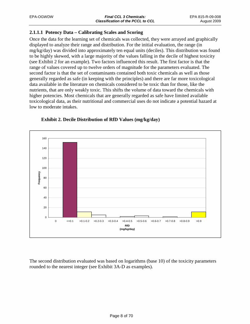
Exhibit 2. Decile Distribution of RfD Values (mg/kg/day)
160
140
120
100
80
60
40
20
0
Freq
uenc
y
0 <=0.1 >0.1-0.2 >0.2-0.3 >0.3-0.4 >0.4-0.5 >0.5-0.6 >0.6-0.7 >0.7-0.8 >0.8-0.9 >0.9
RfD (mg/kg/day)
2.1.1.1 Potency Data – Calibrating Scales and Scoring Once the data for the learning set of chemicals was collected, they were arrayed and graphically displayed to analyze their range and distribution. For the initial evaluation, the range (in mg/kg/day) was divided into approximately ten equal units (deciles). This distribution was found to be highly skewed, with a large majority of the values falling in the decile of highest toxicity (see Exhibit 2 for an example). Two factors influenced this result. The first factor is that the range of values covered up to twelve orders of magnitude for the parameters evaluated. The second factor is that the set of contaminants contained both toxic chemicals as well as those generally regarded as safe (in keeping with the principles) and there are far more toxicological data available in the literature on chemicals considered to be toxic than for those, like the nutrients, that are only weakly toxic. This shifts the volume of data toward the chemicals with higher potencies. Most chemicals that are generally regarded as safe have limited available toxicological data, as their nutritional and commercial uses do not indicate a potential hazard at low to moderate intakes.
The second distribution evaluated was based on logarithms (base 10) of the toxicity parameters rounded to the nearest integer (see Exhibit 3A-D as examples).

EPA-OGWDW Final CCL 3 Chemicals: EPA 815-R-09-008
Classification of the PCCL to CCL August 2009
Page 9 of 70
Exhibit 3A. Logarithmic Distribution of RfD Values
80
70
60
50
<= -6 -5 -4 -3 -2 -1 0 1 2 3 4 More
Round(Log10(RfD))
Freq
uenc
y
40
30
20
10
0
Exhibit 3B. Logarithmic Distribution of NOAEL Values
0
5
10
15
20
25
30
35
40
45
-5 -4 -3 -2 -1 0 1 2 3 4 5 More
Round(Log10(NOAEL))
Freq
uenc
y

EPA-OGWDW Final CCL 3 Chemicals: EPA 815-R-09-008
Classification of the PCCL to CCL August 2009
Page 10 of 70
Exhibit 3C. Logarithmic Distribution of LOAEL Values
0
5
10
15
20
25
30
35
40
45
<= -5 -4 -3 -2 -1 0 1 2 3 4 5 More
Round(Log10(LOAEL))
Freq
uenc
y
Exhibit 3D. Logarithmic Distribution of LD50 Values
0
10
20
30
40
50
60
70
80
-2 -1 0 1 2 3 4 5 6 7 8 More Round(Log10(LD50))
Freq
uenc
y
EPA-OGWDW Final CCL 3 Chemicals: EPA 815-R-09-008
Classification of the PCCL to CCL August 2009
Page 11 of 70
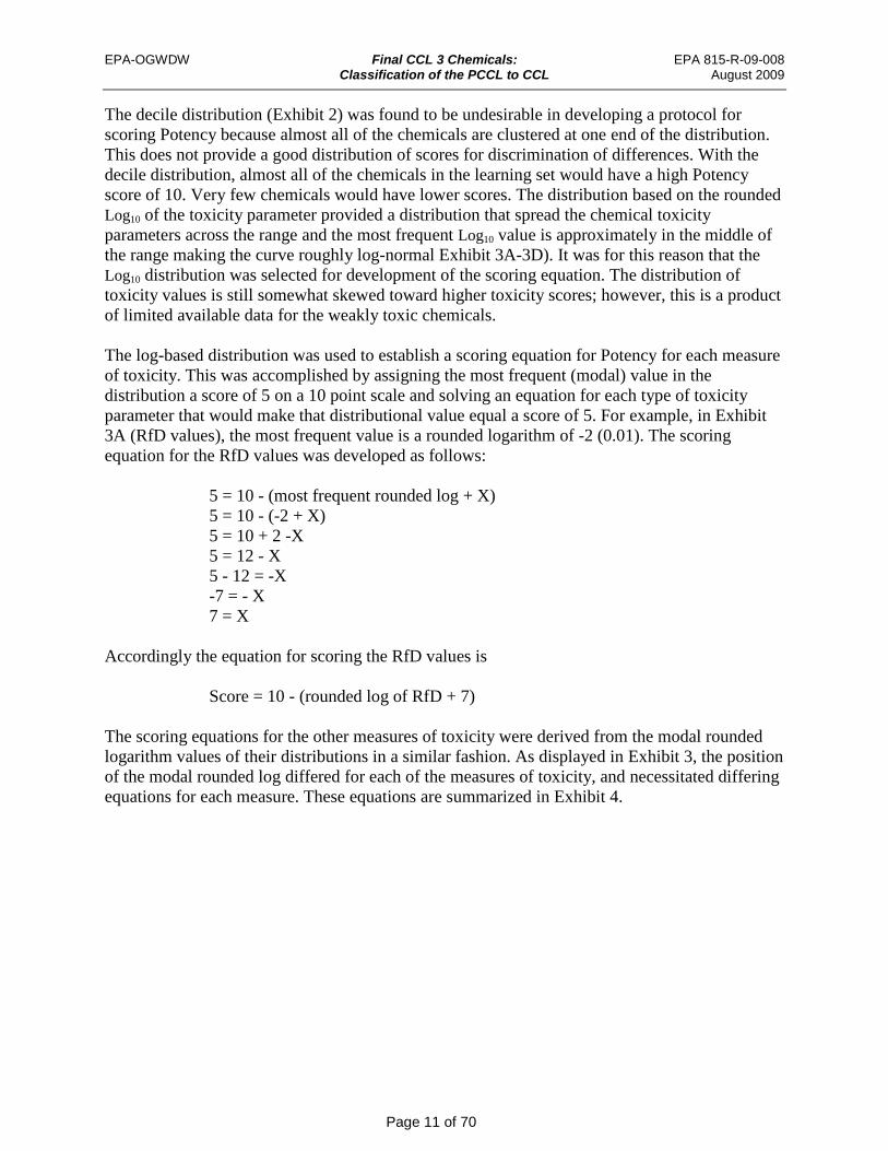
The decile distribution (Exhibit 2) was found to be undesirable in developing a protocol for scoring Potency because almost all of the chemicals are clustered at one end of the distribution. This does not provide a good distribution of scores for discrimination of differences. With the decile distribution, almost all of the chemicals in the learning set would have a high Potency score of 10. Very few chemicals would have lower scores. The distribution based on the rounded Log10 of the toxicity parameter provided a distribution that spread the chemical toxicity parameters across the range and the most frequent Log10 value is approximately in the middle of the range making the curve roughly log-normal Exhibit 3A-3D). It was for this reason that the Log10 distribution was selected for development of the scoring equation. The distribution of toxicity values is still somewhat skewed toward higher toxicity scores; however, this is a product of limited available data for the weakly toxic chemicals.
The log-based distribution was used to establish a scoring equation for Potency for each measure of toxicity. This was accomplished by assigning the most frequent (modal) value in the distribution a score of 5 on a 10 point scale and solving an equation for each type of toxicity parameter that would make that distributional value equal a score of 5. For example, in Exhibit 3A (RfD values), the most frequent value is a rounded logarithm of -2 (0.01). The scoring equation for the RfD values was developed as follows:
5 = 10 - (most frequent rounded log + X) 5 = 10 - (-2 + X) 5 = 10 + 2 -X 5 = 12 - X 5 - 12 = -X -7 = - X 7 = X
Accordingly the equation for scoring the RfD values is
Score = 10 - (rounded log of RfD + 7)
The scoring equations for the other measures of toxicity were derived from the modal rounded logarithm values of their distributions in a similar fashion. As displayed in Exhibit 3, the position of the modal rounded log differed for each of the measures of toxicity, and necessitated differing equations for each measure. These equations are summarized in Exhibit 4.
EPA-OGWDW Final CCL 3 Chemicals: EPA 815-R-09-008
Classification of the PCCL to CCL August 2009
Page 12 of 70
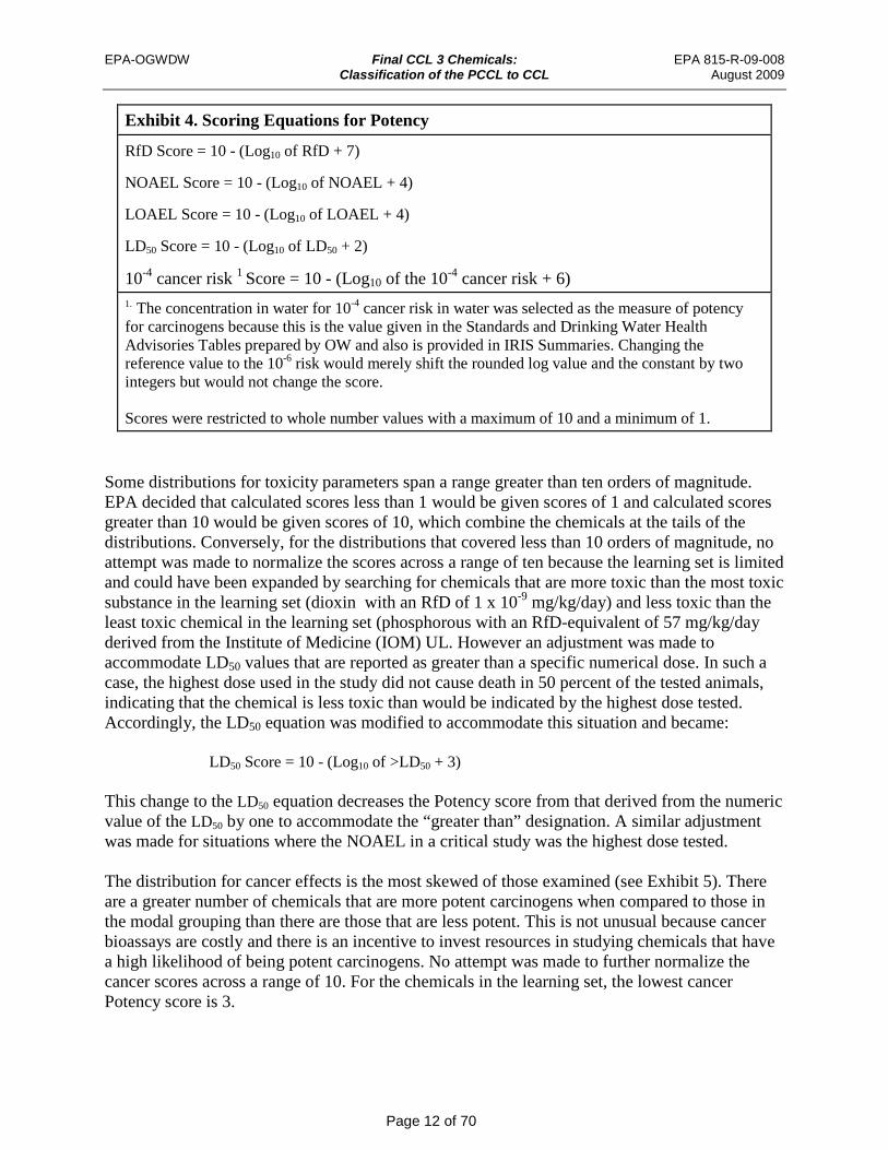
Exhibit 4. Scoring Equations for Potency
RfD Score = 10 - (Log10 of RfD + 7)
NOAEL Score = 10 - (Log10 of NOAEL + 4)
LOAEL Score = 10 - (Log10 of LOAEL + 4)
LD50 Score = 10 - (Log10 of LD50 + 2)
10-4 cancer risk 1 Score = 10 - (Log10 of the 10-4 cancer risk + 6) 1. The concentration in water for 10-4 cancer risk in water was selected as the measure of potency for carcinogens because this is the value given in the Standards and Drinking Water Health Advisories Tables prepared by OW and also is provided in IRIS Summaries. Changing the reference value to the 10-6 risk would merely shift the rounded log value and the constant by two integers but would not change the score.
Scores were restricted to whole number values with a maximum of 10 and a minimum of 1.
Some distributions for toxicity parameters span a range greater than ten orders of magnitude. EPA decided that calculated scores less than 1 would be given scores of 1 and calculated scores greater than 10 would be given scores of 10, which combine the chemicals at the tails of the distributions. Conversely, for the distributions that covered less than 10 orders of magnitude, no attempt was made to normalize the scores across a range of ten because the learning set is limited and could have been expanded by searching for chemicals that are more toxic than the most toxic substance in the learning set (dioxin with an RfD of 1 x 10⁻⁹ mg/kg/day) and less toxic than the least toxic chemical in the learning set (phosphorous with an RfD-equivalent of 57 mg/kg/day derived from the Institute of Medicine (IOM) UL. However an adjustment was made to accommodate LD50 values that are reported as greater than a specific numerical dose. In such a case, the highest dose used in the study did not cause death in 50 percent of the tested animals, indicating that the chemical is less toxic than would be indicated by the highest dose tested. Accordingly, the LD50 equation was modified to accommodate this situation and became:
LD50 Score = 10 - (Log10 of >LD50 + 3)
This change to the LD50 equation decreases the Potency score from that derived from the numeric value of the LD50 by one to accommodate the “greater than” designation. A similar adjustment was made for situations where the NOAEL in a critical study was the highest dose tested.
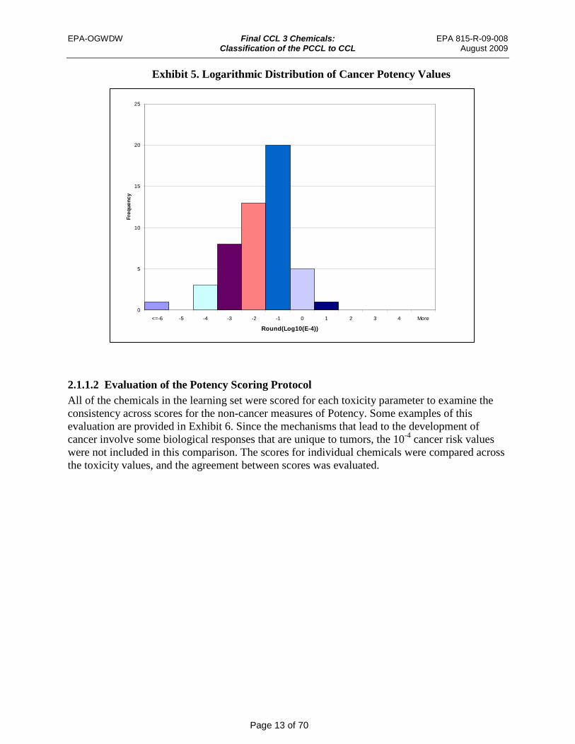
The distribution for cancer effects is the most skewed of those examined (see Exhibit 5). There are a greater number of chemicals that are more potent carcinogens when compared to those in the modal grouping than there are those that are less potent. This is not unusual because cancer bioassays are costly and there is an incentive to invest resources in studying chemicals that have a high likelihood of being potent carcinogens. No attempt was made to further normalize the cancer scores across a range of 10. For the chemicals in the learning set, the lowest cancer Potency score is 3.
EPA-OGWDW Final CCL 3 Chemicals: EPA 815-R-09-008
Classification of the PCCL to CCL August 2009
Page 13 of 70
Exhibit 5. Logarithmic Distribution of Cancer Potency Values
0
5
10
15
20
25
<=-6 -5 -4 -3 -2 -1 0 1 2 3 4 More
Round(Log10(E-4))
Freq
uenc
y
2.1.1.2 Evaluation of the Potency Scoring Protocol All of the chemicals in the learning set were scored for each toxicity parameter to examine the consistency across scores for the non-cancer measures of Potency. Some examples of this evaluation are provided in Exhibit 6. Since the mechanisms that lead to the development of cancer involve some biological responses that are unique to tumors, the 10-4 cancer risk values were not included in this comparison. The scores for individual chemicals were compared across the toxicity values, and the agreement between scores was evaluated.

EPA-OGWDW Final CCL 3 Chemicals: EPA 815-R-09-008
Classification of the PCCL to CCL August 2009
Page 14 of 70
Exhibit 6. Potency Scores for Chemicals in the Learning Set
Chemical RfD NOAEL LOAEL LD50
Calcium (Calcium chloride for LD50) 1 ND 4 5
Cyanazine 6 6 6 6
Dioxin (2,3,7,8-TCDD) 10 ND 10 4
Hexazinone 4 5 4 5
Iodine (Sodium iodide for LD50) 5 8 8 4
Methyl ethyl ketone 3 3 3 5
Methyl parathion 7 8 7 7
Naphthalene 5 4 4 5
Phenol 4 4 4 5
Vitamin D 6 9 9 ND
ND = No data
In addition, the scoring equations were applied to selected chemicals that were not in the learning set using data available in the Agency of Toxic Substances and Disease Registry (ATSDR) Toxicological Profiles. Those results are summarized in Exhibit 7. The scores were evaluated for consistency across parameters.
Exhibit 7. Potency Scores for Chemicals Not in the Learning Set
Chemical/ Potency Scores
RfD-equivalent (mg/kg/day)
NOAEL (mg/kg/day)
LOAEL (mg/kg/day)
LD50 (mg/kg)
Acrylonitrile 4 5 5 6 Ethion 6 7 6 6 Malathion 5 6 5 5 Endosulfan 6 7 ND 5 ND = No Data
The agreement of non-cancer scores across the RfD, NOAEL, LOAEL and LD50 inputs was evaluated. There were 216 chemicals in the learning set; 13.5 percent of those with multiple non-cancer scores had identical scores across all parameters (see cyanazine in Exhibit 6). For 54.6 percent, the scores deviated by 1 integer (see hexazinone in Exhibit 6); 20.5 percent deviated by 2 integers (see methyl ethyl ketone in Exhibit 6). There was a 3-integer deviation for only 9.7 percent, and the majority of those were inorganic compounds (see iodine [sodium iodide] in Exhibit 6). Only 1.6 percent deviated by more than 3 integers (see dioxin in Exhibit 6). Scores deviated by two integers or less for 88.6 percent of the chemicals. The difference between scores

EPA-OGWDW Final CCL 3 Chemicals: EPA 815-R-09-008
Classification of the PCCL to CCL August 2009
Page 15 of 70
for a given compound was greatest for the relatively non-toxic chemicals. In almost all cases the NOAEL and LOAEL scores were higher than the RfD score, effectively negating the concerns that the inclusion of uncertainty factors in the calculation of the RfD would inflate the Potency score. For those chemicals with low uncertainty factors the NOAEL or LOAEL scores were often 3 or more integers higher than the RfD scores (see calcium chloride and vitamin D in Exhibit 6). Since most chemicals with RfD values are also likely to have NOAEL, LOAEL, and/or LD50 values, a policy decision was needed with regard to how one should select the parameter used to score for a non-cancer endpoint. Since there is a general consistency among scores, EPA determined that a hierarchy of RfD> NOAEL> LOAEL> LD50 would be used. In cases where a NOAEL is higher than the lowest LOAEL, the LOAEL would be used in its place. This hierarchy gives preference to the Potency value with the richest supporting da ta set (the RfD or equivalent values) and the lowest ranking to the LD50 because it is a measure of acute rather than chronic toxicity. When comparing cancer and non-cancer scores, it was determined that the end point (cancer or non-cancer) that provided the highest measure of Potency would be used to score the candidate. Similar to the screening pr otocols, EPA applied the potency scoring protocol for LOAELs to contaminants with MRDDs. The Agency did conduct additional searches to identify the best available information to characterize the potency and severity for chemicals on the PCCL, including pharmaceuticals. If additional information was not found, the Agency relied on the data used in the screening step. These evaluations were used to develop the scales and hierarchy of data used in the Potency Scoring Protocol, which is presented in Appendix A . 2.1.2 Severity Severity refers to the relative impact of an adverse physiological change caused by a xenobiotic chemical in humans or animals on the ability of the human or animal to function and survive in the environment. The sixteenth century physician, Paracelsus, provided the underlying principle for the toxicological sciences with the axiom “the dose makes the poison.” Just as toxicity increases with dose, so too does the Severity of the observed effect, in most cases. A low dose effect could be a simple increase in liver weight while the same chemical at a higher dose could cause cirrhosis of the liver. For that reason, the measure of Severity that will be used for scoring in the CCL process is the effect or effects seen at the LOAEL. Restricting Severity scores to the effects occurring at the LOAEL ties them to the data used to derive the Potency score – the type of data likely to be available for CCL candidates. This approach is consistent with the advice provided by the NRC and NDWAC (NRC 2001, NDWAC 2004). The Severity measures that will be used for CCL scoring differ from those used for Potency, Prevalence, and Magnitude because they are descriptive rather than quantitative. Accordingly, they are less amenable to automation and often require more scientific judgment in their application. The sections that follow describe the approach that was used to derive the scoring protocol for Severity and to evaluate its performance.

EPA-OGWDW Final CCL 3 Chemicals: EPA 815-R-09-008
Classification of the PCCL to CCL August 2009
Page 16 of 70
Exhibit 8. NRC Severity Scoring Proposal Score Description 0 No effect 1 Changes in organ weights with minimal clinical significance 2 Biochemical changes with minimal clinical significance 3 Pathology of minimum clinical importance (e.g., fluorosis, warts, common cold) 4 Cellular changes that could lead to disease; minimum functional change 5 Significant functional changes that are reversible (e.g., diarrhea) 6 Irreversible changes; treatable disease 7 Single organ system pathology and function loss 8 Multiple organ system pathology and function loss 9 Disease likely leading to death 10 Death
2.1.2.1 Severity – Scales and Scoring In developing the protocol for scoring Severity, EPA began with the system used by the NRC (2001) for their case study on methods for selecting a CCL from a PCCL. The NRC Severity scoring protocol was based on the anticipated clinical impact of the most sensitive endpoint in affected individuals. The NRC prototype for scoring Severity is provided in Exhibit 8.
In trying to apply the NRC Severity prototype using the critical effects from EPA IRIS Health Risk Assessments, EPA toxicologists encountered difficulty because of the clinical components of the prototype. It was difficult to determine clinical outcomes such as function loss, treatability, or potential for mortality from the critical effects identified in IRIS. In addition, some of the features of a clinical progression could be influenced by the availability and affordability of treatment. EPA decided that it would not be appropriate to use a scoring scheme that had economic and environmental justice implications. The critical effect data for PCCL contaminants will, in most cases, be expressed using terminology very similar to the terminology found in the IRIS database. Accordingly, critical effects of 100 IRIS chemicals were compiled and grouped into categories by EPA toxicologists. These categories were, in turn, used to build a scoring scale that applied some of the rationale reflected in the NRC prototype, but utilized the critical effects information most likely to be available from databases such as IRIS, which eliminated outcome judgments that would confound the scoring process. In this exercise, some difficulties were encountered in scoring Severity, particularly with assigning the middle score categories (3, 4, 5, and 6) and with classifying different types of cancer. Accordingly, the scoring protocol was modified again to try to provide better discrimination between the effects associated with the middle scores and remove the medical treatment considerations. Two new scoring options were developed. One was a nine-point scheme and the other a five-point scheme.

EPA-OGWDW Final CCL 3 Chemicals: EPA 815-R-09-008
Classification of the PCCL to CCL August 2009
Page 17 of 70
Testing of the two new scoring schemes was conducted by EPA toxicologists in the Health and Ecological Criteria Division of the Office of Water. Each toxicologist was presented with all the critical effects given in IRIS with no knowledge of the chemical or chemicals to which they were attached and the revised scoring protocols. They were asked to independently score the large group of critical effect descriptions. The toxicologists met as a group to compare scores and reach consensus on the score and category that is best suited for each critical effect. The five-point scale was compared to the nine-point scale. After completion of this exercise, the nine-point scale displayed in Exhibit 9 was selected based on its ease of use, more transparent clustering of effects within scoring categories, and consistency across the individual scores assigned by toxicologists.
Exhibit 9. Final Nine-Point Scoring Protocol for Severity
Score Critical Effect Interpretation
1 No adverse effect --------
2 Cosmetic effects Considers those effects that alter the appearance of the body without affecting structure or functions
3 Reversible effects; differences in organ weights, body weights or changes in biochemical parameters with minimal clinical significance
Transient, adaptive effects
4 Cellular/physiological changes that could lead to disorders (risk factors or precursor effects)
Considers cellular/physiological changes in the body that are used as indicators of possible adverse systemic damage
5 Significant functional changes that are reversible or permanent changes of minimal toxicological significance.
Considers those disorders in which the removal of chemical exposure will restore health back to prior condition
6 Significant, irreversible, non-lethal conditions or disorders
Considers those disorders that persist for over a long period of time but do not lead to death
7 Developmental or reproductive effects leading to major dysfunction
Considers those chemicals that cause developmental effects or that impact the ability of a population to reproduce
8 Tumors or disorders likely leading to death
Considers chemical exposures that result in a fatal disorder and all types of tumors
9 Death

EPA-OGWDW Final CCL 3 Chemicals: EPA 815-R-09-008
Classification of the PCCL to CCL August 2009
Page 18 of 70
The consensus judgment of the EPA toxicologists was used to construct a compendium of nearly 250 critical effect descriptions grouped by their severity scores (e.g., “Chronic irritation without histopathology changes” equals a score of 3). The final Severity protocol and compendium of critical effects are provided in Appendix A. The ordering of the nine-point scale, which clusters developmental and reproductive effects at a score of 7, and assigns tumors or disorders likely leading to death a score of 8 became a point of discussion. Some reviewers of the protocol felt that a separation of developmental and reproductive effects by the seriousness of the outcome was better than the clustered approach. This option was discussed during internal review of model outcomes (Chapter 4) by an internal EPA reviewer panel. The Agency reviewers decided that the benefits of the proposed scale outweighed potential drawbacks. The ability to clearly identify PCCL chemicals with even a slight developmental reproductive or tumorigenic effect through their Severity score is a benefit of the Exhibit 9 scoring system.
The scoring scale’s “uneven steps” were also noted as a point of concern. A detailed exploration of alternative options, which included the collapse or reordering of the categories, resulted in a consensus judgment to retain the current scale. The current Severity scale works well in providing a meaningful categorization of the array of critical effects. Given the range of critical effects that result from a given exposure, it is not possible to have a consistent difference in the Severity of the outcome between each step on the scale. 2.1.2.2 Evaluation of the Severity Scoring Protocol The Severity scoring protocol was evaluated using the group of chemicals that were included in the training data set discussed in Chapter 3 of this report. Evaluation criteria included:
• Ease of scoring using the protocol and critical effect compendium • Correlation of the list or not list decisions made by workgroup members using the written
narrative descriptions of the critical effects with those made with the numeric scores. • Outcomes from the algorithm list/no-list decisions (discussed in Chapter 4) using the
scored data as compared with workgroup’s decisions based on the descriptive data.
During the initial evaluation process several issues were identified. The most challenging issue related to Severity scores derived from LD50 Potency data. According to the scoring protocol, the Severity score for an LD50 Potency value would be based on the outcome of death in the test population and result in a Severity score of 9. The same score of 9 would be given to a LOAEL or RfD from a more chronic study where the critical effect was described as decreased survival or longevity. When the evaluator’s decisions based on descriptive information for both the Potency and Severity were compared to the decisions based on scores, it was apparent that the evaluators looked at the two effects differently. A decrease in survival from a standard chronic study was regarded as a more serious concern than death in a LD50 study where death is the targeted outcome. Several options were considered for solving this problem. The simplest option was to have no Severity score for an LD50 based Potency value. Another option was to retrieve the study that was the basis of the LD50 value and use the critical effect and dose for systemic effects observed rather than death. The last option was to look for a Potency value and critical effect from a toxicity study other than an LD50 study.

EPA-OGWDW Final CCL 3 Chemicals: EPA 815-R-09-008
Classification of the PCCL to CCL August 2009
Page 19 of 70
Experimentation with the three options for Severity based on LD50 values demonstrated that a combination of the second and third options provided a feasible alternative to scoring Severity on the basis of death when the Potency value was an LD50. The option of eliminating the Severity score for an LD50 value was determined to be a poor choice since it fails to make full use of the available data. It was decided that only when attempts failed to identify an alternate study and/or pre-mortality effects in the LD50 study, that an LD50 based score of 9 would be assigned.
A problem was encountered with critical effect information for LOAELs from the RTECS database. This database summarized all effects without specifying which one was the critical effect. In cases where the original data source was available in the supplemental data, it was consulted to identify which effect was critical. When the supplemental data identified a NOAEL for the critical study it replaced the RTECS LOAEL. If the original source could not be accessed, an alternative NOAEL or LOAEL and its critical effect(s) were identified from the supplemental data and replaced the RTECS LOAEL. Two guidelines were applied when choosing the replacement option. In most cases a replacement was made only if the new LOAEL was lower than the RTECS value. However, in some cases the alternate value, although greater than the RTECS LOAEL was chosen because it was from a study that was higher in quality, more accessible and more recent than the RTECS citation. In any case where the RTECS remained the only source for the data, the score for Severity was based on the most serious of the cluster of effects presented.
Some problems with scoring were encountered in cases where critical effects were not included in the critical effect compendium. The compendium of critical effects descriptors was developed to allow people who were not toxicologists to score chemicals based on Severity. In cases where the scorers could not determine a Severity score, the data were submitted to EPA toxicologists. A minimum of three toxicologists scored the critical effect. The consensus score was determined and the critical effect descriptor and its score were added to the critical effect compendium.
One Severity scoring factor that may have had an effect on the correlation between the classification algorithm-based list/no-list decisions (See Chapter 4) and EPA decisions for the Training Data Set was the numeric Severity score of 8 for carcinogens. The only critical effect to score 8 was carcinogenicity. Workgroup members could easily identify carcinogens by their Severity score and possibly placed more emphasis on this result than the other numeric scores. The classification algorithm was less able to do so, particularly for carcinogens with low Potency values. For example, in some cases, the algorithm made a “no-list” decision when the Severity Score was 8 and the expert evaluators made a “list” decision primarily because of the Severity score’s linkage to cancer. This was particularly true in a couple of cases where all the other scored values were identical or close to identical but Severity was a 7 compared to an 8 (cancer). The decisions for the algorithm and EPA matched more closely when Severity was a 7 than when it was an 8 with EPA more likely to choose a list decision for the 8 Severity score than the algorithm.
In most cases, the combination of Potency and Severity scores performed well in EPA exercises used in developing the PCCL to CCL process and the algorithm trials that followed (Chapter 4). Alternative approaches were adopted for dealing with LD50 based Potency values, and critical effect terms that were not initially in the critical effects compendium were added. Finding an alternative to an LD50 Severity score of 9 and consulting supplemental sources for critical effect information increased the effort required to obtain the Severity data, but appeared to function

EPA-OGWDW Final CCL 3 Chemicals: EPA 815-R-09-008
Classification of the PCCL to CCL August 2009
Page 20 of 70
well. These changes are reflected in the Severity Scoring Protocol and Compendium of Critical Effects in Appendix A. 2.2 Occurrence Attributes The attributes selected to define actual or potential occurrence of contaminants in drinking water are Prevalence and Magnitude. Magnitude is related to the quantity (e.g., concentration) of a contaminant that may be in the environment. Prevalence provides a measure of how widespread the occurrence of the contaminant is in the environment. When direct occurrence data are not available, Persistence and Mobility data are used as surrogate indicators of potential occurrence of a contaminant. Persistence-Mobility is defined by chemical properties that measure or estimate environmental fate characteristics of a contaminant and affect their likelihood to occur in the water environment.
Similar to the health effects attributes, the occurrence attributes are interrelated. The data sources and the learning sets used to define and scale Magnitude, Prevalence, and Persistence-Mobility, as well as more details about the individual attributes are described in the following sections. Unlike the health effects attributes, the data elements used to characterize occurrence are not solely based on a disciplined progressive study of the contaminants. The availability of data from surveys of contaminants in ambient and drinking water, the detection limits of analytical methods, limitations in reporting requirements, as well as indirect measures of potential occurrence needed to be considered and evaluated. Data sources that could provide occurrence data ranged from direct measures of concentrations in water to annual measures of environmental release or production.
The most relevant data for characterizing demonstrated occurrence are monitoring studies or surveys designed to assess national occurrence in drinking water. Finished drinking water occurrence data sources that have been compiled include the Unregulated Contaminant Monitoring Regulations (UCMR), t he National Drinking Water Contaminant Occurrence Database (NCOD) (Round 1 and Round 2 unregulated contaminant data), and the National Inorganic and Radionuclide Survey (NIRS).
Finished water occurrence data are often not available for many chemicals; therefore, other types of data that provide the measures of potential occurrence in Public water systems (PWSs) need to be considered. EPA identified national monitoring studies of occurrence in ambient waters, which may be the eventual source waters for drinking water supplies. Two US Geological Survey (USGS) data sources provide information on source water occurrence for CCL: the National Water Quality Assessment Program (NAWQA) and studies related to the National Reconnaissance of Emerging Contaminants. These sources provide direct measures of occurrence in potential source water and indicate possible occurrence in PWSs.
Many of the chemicals evaluated through the CCL process will not have direct water measurements (finished or ambient). Other available sources that provide data about the potential for drinking water occurrence include:
• the EPA Toxics Release Inventory (TRI), that reports annual volumes of chemicals released from industrial applications and the number of states in which those releases occur;

EPA-OGWDW Final CCL 3 Chemicals: EPA 815-R-09-008
Classification of the PCCL to CCL August 2009
Page 21 of 70
• the National Center for Food and Agricultural Policy’s National Pesticide Use Database that provides estimates of the amount of pesticide applied and the number of states in which it is applied; and
• EPA’s Chemical Update System/Inventory Update Rule (CUS/IUR), a source for annual production volume data under the Toxic Substances Control Act. Note the CUS/IUR data are categorical (i.e., chemicals are in categories with a range of production values, such as 500,000 to 1,000,000 pounds).
2.2.1 Prevalence and Magnitude Data Elements A learning data set of 207 chemicals was compiled and used to develop and calibrate scales for scoring the Magnitude and Prevalence attributes. Due to the linkage of the data used, the scaling and scoring evaluations were performed concurrently. The linkage between Magnitude and Prevalence measures is shown in Exhibit 10. The Magnitude measure indicates the median concentration of detections in water or the total pounds of the chemical released into the environment. The median was selected over mean because it typically is a more stable estimate of central tendency in environmental occurrence data. Outliers have strong i nfluence on means, often to the extent that the mean is greater than all but the maximum value (particularly when only detections are used in the calculation). The median of detections was selected over the median of all measurements in water because all measurements would include non-detections. Non-detections either signify that the chemical is not occurring or the analytical method is unable to measure the chemical below the detection limit. The inclusion of non-detections reduces the median value and, for the majority of environmental chemicals, t he median would be a less than value (i.e., < the reporting or a “non-detect” value). This would provide little information and limited discrimination among the chemicals. Prevalence uses the same data source as Magnitude. The linked Prevalence measure provides an indicator of how widely the contaminant may be present; in general Prevalence shows the proportion of monitoring sites or states with detections or releases.
Exhibit 10. Relationship of Data Elements Used to Score Magnitude and Prevalence.
Magnitude Data Prevalence Data
Median concentration of detections from finished water systems.
Percent of finished water systems nationally with detections of a contaminant.
Median concentration of detections from ambient water sites.
Percent of ambient water sites nationally with detections of a contaminant.
Amount of total releases nationally in TRI; annual, in pounds.
Number of states reporting releases of the chemical in the Toxics Release Inventory.
Sections 2.2.2 and 2.2.3 discuss the approach used to develop and calibrate the scales for scoring Prevalence, and Section 2.2.4 through 2.2.7 discusses the approach for Magnitude including the use of Persistence and Mobility Scores as a surrogate for Magnitude when Production volume is used for Prevalence.

EPA-OGWDW Final CCL 3 Chemicals: EPA 815-R-09-008
Classification of the PCCL to CCL August 2009
Page 22 of 70
2.2.2 Prevalence - Calibrating Scales and Scoring Prevalence is a measure of a contaminant’s occurrence across the United States. It uses measures such as:
• Contaminant detections from Drinking Water Monitoring Programs • Contaminant detections from Ambient Water Monitoring • States where pesticides are applied • States reporting releases of a given chemical to the environment • Production of commodity chemicals in pounds per year
These Prevalence measures have finite ranges such as zero to 100 percent of PWSs or 1 to 50 states depending on the reporting r equirements of the available data source. Accordingly, transformations to log-based distributions are not necessary. The scaling analyses for Prevalence focused on establishing gr oupings of the chemicals across the scoring scale.
The analyses began with equal bin distributions. Both 100 percent of sites with detections and 50 states with releases divide equally into ten bins based on deciles. In the case of Prevalence, the bins provided a fairly good fit to the distribution. However, they still required some adjustment because the equal bins had a tendency to segregate contaminants by type. Contaminants with the highest percent detections scoring a 9 or 10 were naturally occurring inorganic contaminants. For example, in the National Inorganic and Radionuclide Survey for ground water, ions such as sodium, calcium, and iron were all detected in ≥ 90% of the groundwater systems sampled. Contaminants with the highest releases were mostly the high-use pesticides applied in nearly all the agricultural states or high-use commodity chemicals with reported discharges from manufacturing or distribution sites in a large number of states such as the Benzene, ethyl benzene, toluene, and xylene impurities in petroleum products.
Creating ten equal bins from the number of states with environmental releases resulted in a scale where a Prevalence score of 10 meant that releases had to be reported from 45 or more States. EPA revised the scale for release data so that if more than half the states (25) reported releases the chemical would receive a Prevalence score of 10 and indicate that the contaminants potential for occurrence was relatively high. The percent of detections in finished and ambient water (i.e. percent of systems/sites) were also adjusted to ensure that the most widely detected organic chemicals received more representative scores when compared to the naturally occurring inorganic compounds (IOCs). Among occurrence data elements, the linkage between the Prevalence measures and Magnitude measures works well for the water measurements and environmental release measures. It does not work well in the cases when only annual Production data are available. The Production data provide a measure of pounds of a chemical product produced annually in the United States but these data do not provide a linked measure such as the number of states in which it is produced or used. This production rate represents the commercial importance of the chemical to some extent. Since high production tonnage suggests wide use of a commodity chemical, EPA decided that production data would be used as a measure for likely Prevalence across the country. For example, a chemical produced at a billion pounds per year is more likely to be used and released more widely than a compound produced at only 10,000 pounds per year. Experimentation to examine the correlation of Prevalence scores based on measures of detections in water and the
EPA-OGWDW Final CCL 3 Chemicals: EPA 815-R-09-008
Classification of the PCCL to CCL August 2009
Page 23 of 70
number of states receiving environmental releases, based on production, supported this hypothesis. Correlations were only fair to good bu t justified the use of production data as a measure of Prevalence when other data on the spatial spread of a contaminant across the United States are not available.
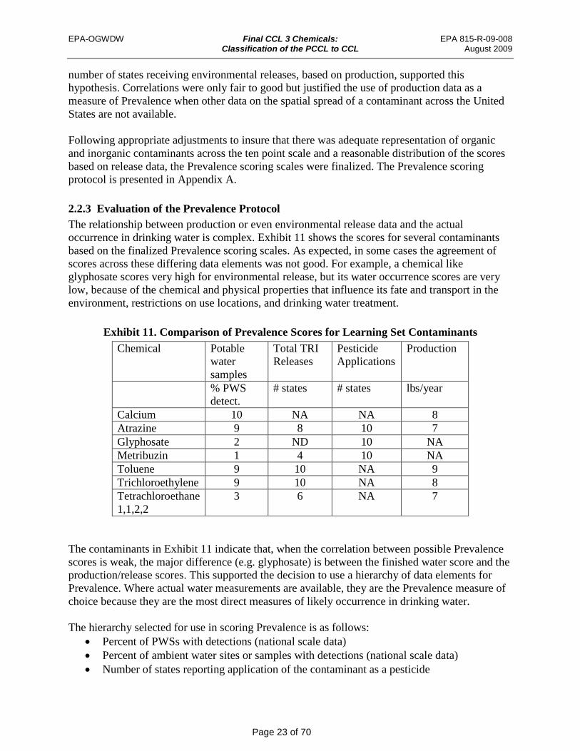
Following a ppropriate adjustments to insure that there was adequate representation of organic and inorganic contaminants across the ten point scale and a reasonable distribution of the scores based on release data, the Prevalence scoring scales were finalized. The Prevalence scoring protocol is presented in Appendix A. 2.2.3 Evaluation of the Prevalence Protocol The relationship between production or even environmental release data and the actual occurrence in drinking water is complex. Exhibit 11 shows the scores for several contaminants based on the finalized Prevalence scoring scales. As expected, in some cases the agreement of scores across these differing data elements was not good. For example, a chemical like glyphosate scores very high for environmental release, but its water occurrence scores are very low, because of the chemical and physical properties that influence its fate and transport in the environment, restrictions on use locations, a nd drinking water treatment.
Exhibit 11. Comparison of Prevalence Scores for Learning Set Contaminants Chemical Potable Total TRI Pesticide Production
water Releases Applications samples
% PWS
# states # states lbs/year detect.
Calcium 10 Atrazine 9
Glyphosate 2 Metribuzin 1
Toluene 9 Trichloroethylene 9
Tetrachloroethane 3
NA 8 ND
4 10 10 6
NA 10 10 10 NA NA NA
8 7 NA NA
9 8 7
1,1,2,2
The contaminants in Exhibit 11 indicate that, when the correlation between possible Prevalence scores is weak, the major difference (e.g. glyphosate) is between the finished water score and the production/release scores. This supported the decision to use a hierarchy of data elements for Prevalence. Where actual water measurements are available, they are the Prevalence measure of choice because they are the most direct measures of likely occurrence in drinking water. The hierarchy selected for use in scoring Prevalence is as follows:
• Percent of PWSs with detections (national scale data) • Percent of ambient water sites or samples with detections (national scale data) • Number of states reporting application of the contaminant as a pesticide

EPA-OGWDW Final CCL 3 Chemicals: EPA 815-R-09-008
Classification of the PCCL to CCL August 2009
Page 24 of 70
• Number of states reporting releases (total) of the chemical • Production volume in pounds per year
2.2.4 Magnitude - Calibrating Scales and Scoring To scale the Magnitude attribute, an evaluation to identify possible correlations among data elements was conducted. First, a comprehensive universe of finished water quality data was compiled, including the national occurrence database of regulated contaminants (compiled for the first 6-Year Regulatory Review), the historic data from various unregulated contaminant monitoring programs (noted as NCOD Rounds 1 and 2, above), and the data from NIRS. This provided a comprehensive array of data covering the expected distribution range of Magnitude for any new contaminant, ranging f rom high median concentrations for some naturally occurring inorganic ions or elements to non-detect values for some trace organic chemicals.
The NRC (2001) had initially recommended that Magnitude be scored based on its relationship to Potency. In their pilot study they proposed that the magnitude score be the square root of the median concentration, (based on its position in a decile distribution) times the potency score. A median concentration that fell within the lowest decile of the distribution would receive a 1 and that in the highest decile a 10 for the calculation. EPA evaluated the NRC approach to scoring Magnitude and found that it was not feasible for the following r easons:
• The NRC equation cannot be applied when the Magnitude data are based on environmental release or chemical/physical properties.
• A decile distribution for the median concentration values results in low scores for almost all organic chemicals because of the high concentration of geochemical inorganic contaminants present in water (see Exhibit 12)
• Application of the NRC equation did not provide a good measure of relative Magnitude (see aldrin and sodium in Exhibit 12). A high concentration, low Potency combination can receive the same score as a low concentration, high Potency combination.
To examine the efficacy of the NRC approach, EPA applied it to six of the chemicals from CCL 1 for which regulatory determinations had been made and t he magnitude scores, thus, had the necessary Potency and occurrence data. The results of that evaluation are summarized in Exhibit 12.

EPA-OGWDW Final CCL 3 Chemicals: EPA 815-R-09-008
Classification of the PCCL to CCL August 2009
Page 25 of 70
Exhibit 12. Comparison of the NRC Magnitude Score with the Ratio of the Health Advisory Guideline to the Concentration in Finished Water Contaminant Potency Benchmark Median
Concentration Magnitude Potency
Benchmark: Concentration Ratio1
mg/L Score mg/L Score NRC score
Aldrin 0.000002 10 0.0006 1 3.2 0.003 Hexachlorobutadiene
0.0009 7 0.001 1 2.6 0.9
Manganese 0.3 4 0.01 1 2 30 Metribuzin 0.07 5 0.001 1 2.2 70 Naphthalene 0.1 5 0.001 1 2.2 100 Sodium 120 1 16.4 10 3.2 7.3 1The Potency Benchmark is the Health Advisory guideline (cancer or non-cancer) for a lifetime exposure for all chemicals except sodium. The guideline for sodium is derived from the recommended dietary intake for sodium in adults, 2.4 g/day ÷ 2L/day using a Relative Source Contribution of 10%. The Potency Scores were derived from the RfD-equivalent or 10-4 cancer risk values. The concentration scores were obtained by using sodium as the upper level for the range and dividing the range into deciles as recommended by NRC.
As indicated in Exhibit 12, the NRC score does not display a consistent relationship to the ratio of the potency-based drinking water guideline to the median finished water concentration. Aldrin, the contaminant from Exhibit 12 that is present in drinking water at the levels of greatest concern has the same magnitude score as sodium ion that is only weakly toxic and not present at a concentration of concern for other than those on very low sodium diets. In addition, as mentioned above, the decile distribution of concentrations resulted in a score of 1 for any contaminant present in water at concentrations lower than 1.6 mg/L (one tenth of the sodium concentration). Given this distribution, only inorganic contaminants are likely to receive intermediate scores on the concentration scale. Because of the observed limitations in the NRC proposed approach EPA determined that it was not appropriate for scoring Magnitude.
The second approach that was investigated employed the use of the Health Reference Level (HRL) to establish the scores for Magnitude. For example, the largest dose that received a Potency score of 10 was converted to a mg/L equivalent using the HRL methodology. Anything less than that concentration received a 1 on the Magnitude scale. Each log-based Potency value was paired with a log-based concentration. A Potency score of 10, when paired with any Magnitude score, would be suggestive of concern because the concentration was greater than the Potency. However a Potency score of 8 would only give rise to concern if the Magnitude score was 3 or greater (see Exhibit 13).

EPA-OGWDW Final CCL 3 Chemicals: EPA 815-R-09-008
Classification of the PCCL to CCL August 2009
Page 26 of 70
Exhibit 13. Magnitude Concentrations and Scores Derived from Potency Doses Potency Score
Potency Range mg/kg/day
Concentration equivalent mg/L
Magnitude Score
10 0 to 3.16 x 10⁻⁷ 0 to 2.2 x 10⁻⁶ 1 9 3.17 x 10⁻⁷ to 3.16 x 10⁻⁶ >2.2 x 10⁻⁶ to 2.2 x 10⁻⁵ 2 8 3.17 x 10⁻⁶ to 3.16 x 10⁻⁵ >2.2 x 10⁻⁵ to 2.2 x 10⁻⁴ 3
This second approach to relating Potency and Magnitude proved to be unwieldy because the two scales are inversely related. It was also problematic because it could not be used for Potency values based on NOAELs, LOAELS, and LD50s, or Magnitudes that were not expressed in concentrations terms. It also did not take into account the differences in the HRL determination process for carcinogens versus non-carcinogens.
EPA next explored a variety of potential scales that could be applied to the finished water concentration data without consideration of Potency. EPA converted the finished water data to a standard unit of measure (μg/L) and evaluated several ranges of concentrations to correspond to magnitude scores. Exhibits 14A through 14C illustrate the comparisons of three of the approaches evaluated for the organic and inorganic contaminants. Exhibit 15 shows the differentiation in scores across the three experimental approaches.
The first approach was to develop scales that utilized the array of compiled Magnitude data and 10 bins with approximately equal numbers of contaminants in each bin, referred to as the equal number bins scale in Exhibit 14A. Equal bins did not provide a good dispersion of scores. Accordingly, various log-scale options were explored. The Magnitude data do not range across as many orders of magnitude as the Potency RfD data, so various semi-logarithmic scales were evaluated to better represent the distribution of values across the scale.
In evaluating and developing the calibration scale, the water occurrence data presented a particular challenge because the IOCs tended to skew the results. Many IOCs result from various anthropogenic processes, but most are of geologic origin as well, and they have relatively high measures for both Prevalence and Magnitude compared to most organic chemicals. Hence, for some of the semi-logarithmic Magnitude scales (e.g., Half-Log Option A), the only chemicals that could score high (e.g., a 10 or 9) would be IOCs. Such a scale would depress the score for organic chemicals that are of equally high concern because of their expectedly lower concentrations. One approach that EPA evaluated was using different scales for IOCs and organic chemicals; however, having two scales would make the scoring process overly complex. To keep the process straightforward and transparent it was decided to use one scale for all water data. Accordingly, the scores were distributed across the range of values so that organic contaminants could receive high scores as well as the IOCs. Comparisons and adjustments were made until the current protocols, using a semi-logarithmic scale (Half-Log Option B shown in Exhibit 14C), were selected.

EPA-OGWDW Final CCL 3 Chemicals: EPA 815-R-09-008
Classification of the PCCL to CCL August 2009
Page 27 of 70
50
40
Cou
nt o
f Con
tam
inan
ts
< 0.2
1
0.20-<0.50
2
0.50-<0.51
3
0.51-<0.75
4
0.75-<1.0
5
1.0-<1.01
6
1.01-<1.25
7
1.25-<1.60
8
1.60-<2.50
9
> 2.50
10
30
20
10
0
Category and Break Points µg/L
Organics Count Inorganics Count
Exhibit 14A. Equal Bins Drinking Water Magnitude Scale (ug/L)
Exhibit 14B. Half Log Option A Drinking Water Magnitude Scale (ug/L)
75
60
45
30
15
0 < 0.10 0.10-<0.3 0.3-<1 1-<3 3-<10 10-<30 30-<100 100-<300 300-<1000 > 1,000.0
1 2 3 4 5 6 7 8 9 10
Category and Break Points
Cou
nt o
f Con
tam
inan
ts
Organics Count Inorganics Count

EPA-OGWDW Final CCL 3 Chemicals: EPA 815-R-09-008
Classification of the PCCL to CCL August 2009
Page 28 of 70
Exhibit 14C. Half Log Option B Drinking Water Magnitude Scale (ug/L)
0
15
30
45
60
75
< 0.003 0.003<0.01
0.01-<0.03 0.03-<0.1 0.1-<0.3 0.3-<1.0 1.0-<3.0 3.0-<10.0 10.0-<30.0 > 30.0
1 2 3 4 5 6 7 8 9 10
Cou
nt o
f Con
tam
inan
ts
Category and Break Points
Organics Count Inorganics Count
Exhibit 15. Magnitude Attribute Scores: Example Contaminants Scored by their Median of Detections Using the Various Approaches in Exhibit 14.
Half-Log Half-Log “Bins” Chemical Option A Option B Score Score Score
Hexachlorobutadiene 2 2 5
1,1,2,2-Tetrachloroethane 3 3 6
Boron 10 6 10
Sulfate 10 10 10
Antimony 9 4 7
Ethylbenzene 6 4 6
Endothall 10 6 9
Methyl ethyl ketone 5 3 6
When developing the calibration scales for the release data, the ranges of data were similarly arrayed using a scale based on half-log units with a distribution of scores that reflected the distribution of the data in the learning set.

EPA-OGWDW Final CCL 3 Chemicals: EPA 815-R-09-008
Classification of the PCCL to CCL August 2009
Page 29 of 70
2.2.5 Persistence-Mobility as a Surrogate Measure for Magnitude In cases where production data are the only measure of occurrence, scoring for Prevalence and Magnitude becomes difficult. The NRC discussed Persistence and Mobility as a fifth attribute and had suggested it could be used to predict possible occurrence if other direct measures were not available. In its review, NDWAC suggested that Persistence and Mobility could provide a surrogate measure of Prevalence with production used as a measure of Magnitude. To examine the NDWAC proposal, EPA carried out a series of exercises in which scores for Magnitude derived from concentrations in drinking water and environmental releases were examined to see if they correlated with production scores and with Persistence-Mobility scores calculated using the scoring equation developed by NDWAC. In no case was the correlation as good as one might desire, but it was apparent that the Persistence-Mobility approach showed a better correlation with the Magnitude scores, based on the preferred data elements (concentration/release), than the production information. Accordingly, EPA chose to use Persistence-Mobility as a surrogate measure for Magnitude. Persistence and Mobility are environmental fate parameters. They are considered in combination as a measure of potential occurrence because both transport (i.e. Mobility) and fate (i.e. Persistence) are important when predicting whether a contaminant is likely to be found in water at a specific location, in situations where there is an environmental source for the contaminant. The length of time a chemical remains in the environment before it is degraded (Persistence) affects its importance as a potential drinking water contaminant. Persistence is generally expressed as rate of degradation or half-life (t1/2) indicating, in this case, the length of time required for the chemical to degrade to half its original concentration in the medium of interest (e.g. water). Similarly, the Mobility of a chemical, or its ability to be transported to and in water, affects its potential to reach and dissolve in the source waters for a PWS.
There are a number of data elements that measure the fate of a chemical in the environment. The physical/chemical parameters that are most relevant to the fate in drinking water are summarized in Exhibit 16. The first 4 measures of mobility represent the equilibrium ratio for the partitioning of the contaminant from one medium to another: Koc (sediment: water), Kow (octanol: water), Kd (soil: water) and Henry’s Law Coefficient (air: water). Koc, Kow and Kd are sometimes expressed as logs of the original measurements. The measures of persistence each reflect the time the chemical will remain unchanged in the environment.
Exhibit 16. Mobility and Persistence Data Elements MOBILITY PERSISTENCE
Organic Carbon Partition Coefficient (Koc) Half-Life
Octanol/Water Partition Coefficient (Kow) Measured Degradation Rate
Soil/Water Distribution Coefficient (Kd) Modeled Degradation Rate
Henry's Law Coefficient (KH)
Solubility

EPA-OGWDW Final CCL 3 Chemicals: EPA 815-R-09-008
Classification of the PCCL to CCL August 2009
Page 30 of 70
The data elements listed in the table above are arranged in hierarchical order, with the most desirable at the top (i.e., the first data to be used if available). Organic Carbon Partitioning Coefficient (Koc) is one of the most common indicators of the mobility of a chemical in water. A high Koc increases the probability that, once a chemical reaches a receiving water body, it will remain bound to sediments or adjacent soils, and thus, slowly partition from the sediment to the water column. A high Koc favors the presence of the contaminant in water for a long time but at low concentrations since the Koc will favor the sediment over the water. A high solubility favors rapid dissolution in the water body from a nearby source and potentially high concentrations if the water source is confined and the environmental release substantial. 2.2.6 Persistence-Mobility Data – Calibrating Scales and Scoring Many of the measurements of environmental fate properties vary depending on the actual field or laboratory conditions. Some are reported in standard data sources only as ranges, or categorical descriptions. Scoring was further complicated by the fact that two separate environmental fate parameters were used in the scoring of the one attribute. Accordingly, EPA selected the approach proposed by NRC and supported by the NDWAC for using the Persistence-Mobility information after experimenting with several other approaches. The Persistence and Mobility data were arrayed, or partitioned into relatively simple lowmedium-high categories as suggested by NRC. Published definitions for the categories were used, such as the categories for Koc from Fetter, 1994 and the classifications for the octanol water partition coefficient (Kow) from Lyman, et al, 1990. The categories are given values of 1, 2, or 3 based on the ranking of the measurement from low to high. The persistence value is averaged with the mobility value and a multiplier (10/3) is used to translate the score to a 10 point scale (see the Persistence-Mobility Protocol in Appendix A, for details). Since the persistence and mobility data are being used as a measure of Magnitude, a low ranking (1) for a parameter is one that will minimize the concentration in water and a high ranking (3) is one that will maximize the concentration. For example, a high Koc means that the distribution between the water column and sediment favors the sediment and is ranked a low, while a lower Koc means that the ratio of a contaminant in sediment to that in the water allows a larger portion of the total to be in the water and is ranked as high. As mentioned above, EPA undertook a series of evaluations to compare the Persistence-Mobility scores for selected contaminants to the Magnitude scores derived from the preferred data elements (concentrations in water or environmental releases). Often, data were not available for a half-life or a measured degradation rate for the Persistence value. In these cases, EPA’s PBT Profiler was tested and added to the Persistence protocol to ensure both Mobility and Persistence data were used to calculate the attribute score (www.pbtprofile.net).
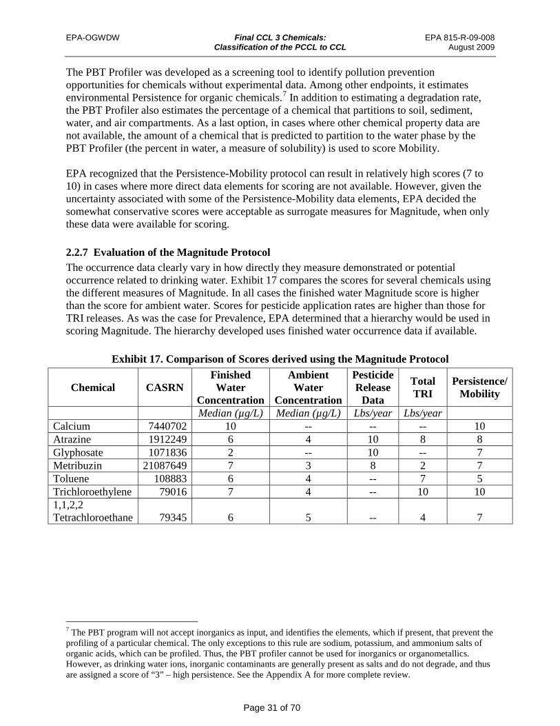
EPA-OGWDW Final CCL 3 Chemicals: EPA 815-R-09-008
Classification of the PCCL to CCL August 2009
Page 31 of 70
The PBT Profiler was developed as a screening tool to identify pollution prevention opportunities for chemicals without experimental data. Among other endpoints, it estimates environmental Persistence for organic chemicals.7 In addition to estimating a degradation rate, the PBT Profiler also estimates the percentage of a chemical that partitions to soil, sediment, water, and air compartments. As a last option, in cases where other chemical property data are not available, the amount of a chemical that is predicted to partition to the water phase by the PBT Profiler (the percent in water, a measure of solubility) is used to score Mobility. EPA recognized that the Persistence-Mobility protocol can result in relatively high scores (7 to 10) in cases where more direct data elements for scoring are not available. However, given the uncertainty associated with some of the Persistence-Mobility data elements, EPA decided the somewhat conservative scores were acceptable as surrogate measures for Magnitude, when only these data were available for scoring.
2.2.7 Evaluation of the Magnitude Protocol The occurrence data clearly vary in how directly they measure demonstrated or potential occurrence related to drinking water. Exhibit 17 compares the scores for several chemicals using the different measures of Magnitude. In all cases the finished water Magnitude score is higher than the score for ambient water. Scores for pesticide application rates are higher than those for TRI releases. As was the case for Prevalence, EPA determined that a hierarchy would be used in scoring Magnitude. The hierarchy developed uses finished water occurrence data if available.
Exhibit 17. Comparison of Scores derived using the Magnitude Protocol Finished Ambient Pesticide Total Persistence/ Chemical CASRN Water Water Release TRI Mobility Concentration Concentration Data
Median (µg/L) Median (µg/L) Lbs/year Lbs/year Calcium 7440702 10 - - - 10 Atrazine 1912249 6 4 10 8 8 Glyphosate 1071836 2 - 10 - 7 Metribuzin 21087649 7 3 8 2 7 Toluene 108883 6 4 - 7 5 Trichloroethylene 79016 7 4 - 10 10 1,1,2,2 Tetrachloroethane 79345 6 5 - 4 7
7 The PBT program will not accept inorganics as input, and identifies the elements, which if present, that prevent the profiling of a particular chemical. The only exceptions to this rule are sodium, potassium, and ammonium salts of organic acids, which can be profiled. Thus, the PBT profiler cannot be used for inorganics or organometallics. However, as drinking water ions, inorganic contaminants are generally present as salts and do not degrade, and thus are assigned a score of “3” – high persistence. See the Appendix A for more complete review.

EPA-OGWDW Final CCL 3 Chemicals: EPA 815-R-09-008
Classification of the PCCL to CCL August 2009
Page 32 of 70
The hierarchy suggested for Magnitude draws on the following data sets: • Median concentration of detections from finished water systems • Median concentration of detections from ambient water sites or samples • Amount of pesticide applied • Amount of total releases • Persistence-Mobility data
2.3 Fine Tuning the Protocols As discussed in the previous sections, EPA developed and fine-tuned the Attribute Scoring Protocols through a step-wise process of data selection, data analysis, calibration of scales, and evaluation of the functionality of the scores in PCCL to CCL decision-making. The decision-making component of the process examined the ability of the scored attributes to adequately represent the level of concern about contaminants. The testing also evaluated whether or not the scores provide a consistent input to the decision making portion of the CCL listing process that is relatively independent of the type of input data that provides the basis for the score.
Quality assurance measures utilized comparisons of list - not list determinations by a panel of EPA subject matter experts based on descriptive and quantitative measures of health effects and occurrence (raw data) compared with determinations based on the scored attributes. Differences in decisions were identified. The panel discussed those differences and the rationale they had used to reach decisions based on the raw data versus the scored data. Minor adjustments were made to the scoring protocols based on those discussions.
Using a training data set of contaminants (Chapter 3), blinded test-case decisions made with raw data versus scored results, or decisions based on one data element in a hierarchy versus another, were compared. The results provided a high level of confidence that the scores, while not capturing all information experts used in making de cisions based on raw data, adequately captured the critical relationships that informed “list” versus “don’t list” determinations made by the EPA panel.
3.0 DEFINITIONS AND OVERVIEW OF THE TRAINING DATA SET This chapter describes the process used to identify a set of chemicals to train (or calibrate) the classification models discussed in the next chapter. The raw data, attribute scores, and protocols discussed in chapter 2 were applied to these contaminants and that information is carried forward in the evaluation of classification models discussed in Chapter 4. The training data set (TDS) for chemicals is the set of data used to train (or teach) the classification models to mimic expert list-not list decisions. The TDS used to train the models for CCL 3 w as comprised of 202 discrete sets of attribute scores for contaminants and consensus list-not list decisions made by a team of EPA subject matter experts. Classification models are algorithms that use statistical approaches for pattern recognition and derive mathematical relationships among input variables (measurements or descriptive data) and output from a TDS. For the CCL, the classification models are used to develop a relationship

EPA-OGWDW Final CCL 3 Chemicals: EPA 815-R-09-008
Classification of the PCCL to CCL August 2009
Page 33 of 70
between the contaminant attribute scores (input variables) and the classification of these contaminants into list-not list categories (output). The mathematical relationship between attribute scores and list-not list decisions is determined based on the classification decisions on TDS chemicals and their associated data. Once the TDS is used to train the classification model, the model is then applied to a larger list of contaminants to predict their classifications, list or not list. The process for developing the TDS utilized EPA subject matter experts familiar with the technical aspects of the attribute data and the selection of drinking water contaminants for listing and regulation. The subject matter experts represented drinking water, toxicology, public health, engineering, and statistics disciplines. 3.1 Key Considerations EPA considered the following key factors in developing the training data set:
• Selection of contaminants representing a range of outcomes and decisions likely to be encountered in developing a CCL;
• A variety of input data ensuring adequate coverage of possible attribute scores and combinations of scores;
• Chemicals that, when present in drinking water, would present a meaningful opportunity for public health improvement if regulated; and
• Contaminants that would likely be selected for the PCCL.
3.2 Developing Key Components of the Training Data Set 3.2.1 Attribute Scores Attribute scores are a critical component of the TDS, as mentioned in Chapter 2. The TDS used for training the classification models consisted of attribute scores for 202 contaminants. A set of known chemicals was chosen to develop the TDS and supplemented with a range of attribute scores that represented hypothetical or artificial contaminants. These artificial contaminants were developed to fill voids in the space of possible attribute scores and improve classification model results. 3.2.2 Attribute scores for real contaminants Initially, EPA selected “data rich” contaminants from among regulated contaminants and previous CCLs because they had a range of readily available occurrence and health effects information. EPA drinking water subject matter experts and stakeholders (as part of the NDWAC process) reviewed the initial list of contaminants and identified candidates for the TDS. Based upon an NRC and NDWAC recommendation, EPA also added chemicals “generally regarded as safe” by the U.S. Food and Drug Administration to provide adequate coverage of possible attribute inputs and a range of list-not list decisions. This initial selection process identified 51 chemical contaminants for the TDS. Subsequently, EPA chose 50 additional contaminants from the CCL 3 U niverse. These 50 contaminants were randomly selected from those with high health effects toxicity levels that had

EPA-OGWDW Final CCL 3 Chemicals: EPA 815-R-09-008
Classification of the PCCL to CCL August 2009
Page 34 of 70
occurrence data because they represented contaminants likely to make it to the PCCL. The addition of these 50 contaminants resulted in 101 contaminants with data to score attributes. To aid in the review and evaluation, data summary sheets were prepared for each contaminant that included available health effects, occurrence, and environmental fate data. All the available health effects and occurrence, use, and fate data that could be used to develop the attribute scores for Potency, Severity, Magnitude and Prevalence were included on the individual summary sheets. The data summary sheets are presented in Appendix B. While contaminant names were included in the initial evaluations, EPA subject matter experts found that knowledge of the contaminant name introduced bias into the decision-making process. Subsequently, EPA “blinded” contaminant names or identifiers in contaminant evaluations to increase objectivity and force decisions to be made solely on the available data and associated attribute scores. The names of contaminants were revealed after the “blinded” evaluations. The attribute scores were developed according to the Attribute Scoring Protocols discussed in Chapter 2 and presented in Appendix A. 3.2.3 Attribute scores for hypothetical contaminants The performance of the classification models using the initial TDS gave an indication of gaps in the possible attribute space that the set of 101 TDS contaminants did not adequately cover. This led EPA to add a set of 101 hypothetical contaminants to the TDS. These contaminants had specific combinations of attribute scores designed to fill gaps in the space defined by all possible attribute scores and to improve the performance of the models. EPA identified 16 general ranges of scores using all four attributes and permutations of high or low scores. The majority of these possible scores were selected using L atin hypercube sampling from the set of all possible attribute score combinations, as seen in Exhibit 18 (NIST, 2006) . Five contaminants were selected at random from each of the 16 “cubes” represented by the combinations of high (6-10) and low (1-5) scores for the four attributes. This selection resulted in 80 hypothetical contaminants. Twenty one additional contaminants were deliberately selected to fill in some obvious voids in the 4-attribute space, resulting in 101 artificial contaminants.

EPA-OGWDW Final CCL 3 Chemicals: EPA 815-R-09-008
Classification of the PCCL to CCL August 2009
Page 35 of 70
Exhibit 18. Combinations of low and high attribute scores 1 for the four attributes using Latin Hypercube Sampling.
Potency Severity Prevalence Magnitude Low Low Low Low Low Low Low High Low Low High Low Low Low High High Low High Low Low Low High Low High Low High High Low Low High High High High Low Low Low High Low Low High High Low High Low High Low High High High High Low Low High High Low High High High High Low High High High High
1 Low scores are randomly sampled from the range 1-5. High scores are randomly sampled from the range 6-10.
Exhibit 19 displays the attribute space coverage of the 101 contaminants compared to the attribute space coverage of the TDS of 202 contaminants. The combination of real and artificial contaminants resulted in 202 scored candidates that became the TDS. The total attribute space for a model that includes four attributes with scores from 1 to 10 is 10,000 combinations of possible attribute scores. Each point plotted in Exhibit 19 represents one chemical in the TDS and one of the 10,000 possible combinations of attribute scores.

Exhibit 19. Attribute Space for the 101 TDS compared to that for the 202 TDSColor of square indicates its classification decision. List = red; List? = beige; Not List? = light blue; and Not List = dark blue (also see Exhibit 29).
EPA-OGWDW Final CCL 3 Chemicals: EPA 815-R-09-008 Classification of the PCCL to CCL August 2009
Page 36 of 70

EPA-OGWDW Final CCL 3 Chemicals: EPA 815-R-09-008
Classification of the PCCL to CCL August 2009
Page 37 of 70
This graphical analysis shows five elements of the model results, the four attributes evaluated and the categorical decision (L, L?, NL?, and NL) in a single graph. Note in Exhibit 19 that the vertical and horizontal axes show two attributes on each axis. The attribute scores for Potency are the large squares across the horizontal axis. The corresponding score for Severity is a separate scale within each larger square. That is, each Potency square has a range of Severity scores. Similarly the Prevalence and Magnitude scores are plotted on the vertical axis, Prevalence as the large squares along the vertical axis and Magnitude as a separate square within each larger square. The decision category assigned each potential attribute is color coded (NL decisions are denoted by dark blue, NL? by lighter blue, L? by beige, and L decisions by red). 3.3 Making List-Not list Decisions List-not list decisions are the second key component of the TDS, as mentioned in Chapter 3. The EPA subject matter experts made list-not list decisions on an individual basis and as a group, based on attribute scores and based on data that had not been converted to attribute scores (actual or raw data). The development of the list-not list decisions was an iterative process that incorporated revisions to the attribute scoring protocols, and the final list-not list decisions, as experience was gained by the EPA experts. Differences between the decisions based on the scored attributes and the raw data were resolved by revising the scoring protocols to improve the correlation of scores to the raw data. After evaluating the health effects and occurrence data for each contaminant, each individual subject matter expert made decisions about how to classify the contaminant, and then met as a group to discuss their decisions. Early in the process the subject matter experts recognized that clear list or not list classification decisions could easily be made for some contaminants, but not for other contaminants. The chemicals in the later group were placed into categories of List? (L?) or Not list? (NL?), in which L? signifies that the decision is leaning towards listing but with some uncertainty, and NL? signifies that the decision is leaning towards not listing, but with some uncertainty. These additional two categories were incorporated into the evaluation process. As part of the iterative process, the subject matter experts discussed their classification results and made adjustments to the process, accordingly. When adjustments changed attribute scoring protocols, TDS contaminants were rescored and reevaluated. Individual decisions were made separately based upon either the raw data or attribute scores. Decisions based upon raw data utilized health effects and occurrence data elements, as well as supporting information on fate and uses. For decisions based on attribute scores, only the numeric individual scores were used. The scores were developed from the raw data using the protocols, for Potency, Severity, Prevalence, and Magnitude. In both cases, this evaluation was conducted “blinded,” meaning contaminant names were not shown. Appendix C summarizes decisions based upon raw data and attribute scores. For each contaminant, comparisons were made between the list – not list decisions based upon raw data and those based on scores. Subject matter experts discussed the similarities and differences on an individual contaminant basis, and revised the attribute protocols to reflect decisions made on the actual data (see Chapter 2). Once list or not list classification decisions were made based on the attribute scores using the revised protocols, consensus among the EPA subject matter experts was used as the final decision for each contaminant. This consensus decision was used to train the models and is further discussed in Chapter 4. Consensus decisions were made by averaging the numerical decisions of individual reviewers (L = 4, L? = 3, NL? = 2, and NL=1) and rounding to the
EPA-OGWDW Final CCL 3 Chemicals: EPA 815-R-09-008
Classification of the PCCL to CCL August 2009
Page 38 of 70
nearest integer. The rounded averages became the consensus values used to train and evaluate the models (Chapter 4). Appendix C also provides the consensus decisions for each TDS contaminant.
4.0 PROTOTYPE CLASSIFICATION MODELS AND THE CCL PROCESS The NRC recommended EPA use prototype classification models for CCL selection, citing the limitations of expert processes and other rule-based models. NDWAC agreed that EPA should use a prototype model, also noting that this should improve the reproducibility and transparency in the process. This kind of approach does not eliminate subjectivity but rather, makes the judgments more explicit. Prototype classification models are often described as pattern recognition models. These models develop statistical relationships (to recognize the patterns) among input variables (attributes, discussed in Chapter 2) of drinking water contaminants to predict their classification (“List,” “List?,” “Not List?,” and “Not List”). The model determines the relationship or rule that links the input to the output based on the decisions made on the TDS (Chapter 3) and then uses that relationship to classify PCCL contaminants based on their attribute scores. In its study, the NRC experimented with a linear discriminant model and an artificial neural network (ANN) model to demonstrate the use of classification approaches. EPA, working with NDWAC, identified the following classes of models for evaluation ( NDWAC 2004):
• Artificial Neural Networks, • Classification Decision Trees (with univariate and multivariate splitting rules), • Linear Models, and • Multivariate Adaptive Regression Splines (MARS).
The model evaluation was a two-step process. First was the evaluation and selection of the most appropriate (“best-fit”) model from within each of the model classes. The second step was the evaluation of the performance of the best models selected from each class. Following these evaluations, two of the models were rejected and three were maintained to inform the final expert review process. Artificial Neural Networks (ANNs) - ANNs are information processing models conceptually based on the human nervous system and its learning processes. ANNs apply flexible and often very complex parameterization. Their value is that they use flexible, non-linear functions that can capture almost any kind of underlying relationship between input and output data. For classification purposes, ANNs apply weighting in non-linear functions and do not specify a strict functional form (such as quadratic or cubic equations) as do many statistical models. Classification Decision Trees - The decision tree classifies the sample by devising a series of tests (or rules, from the TDS) that are mutually exclusive in outcome. The graphical tree is derived with a test at a node in the tree with outcomes from the test branching from each node. Hence, in moving through the tree a contaminant encounters the test at a node, and is sent down one branch or another based on how its attribute(s) meets the test criterion, usually a simple inequality, such as is Magnitude < 3.5 (true or false). Eventually the contaminant reaches a

EPA-OGWDW Final CCL 3 Chemicals: EPA 815-R-09-008
Classification of the PCCL to CCL August 2009
terminal node (the last node, that no longer branches) that assigns the classification (e.g., category 2 = NL?). Two types of decision tree models were explored, Classification and Regression Tree (CART) which utilized univariate (one attribute at a time) tests at nodes, and the Quick, Unbiased, Efficient Statistical Tree (QUEST) model, which utilized multivariate (weighted sum of all attributes) tests at all nodes of the tree. Linear Models – General Linear Models - Two types of linear models were tried. A Logistic regression model was applied to deal with CCL’s categorical data. The Logistic model was only attempted using two categories (List and Not List). EPA found that the binary approach was not satisfactory, and moved to a four category approach. Recognizing that the ANN models often employ logistic regression, to avoid duplication, the Logistic model was dropped from the final evaluations. Consequently, the data were adapted for use with a regular Linear Regression model. This model estimates EPA’s average classification (on a scale of 1 to 4; 1 = Not List, 2 = Not List?, etc.) for each contaminant as a linear combination of the contaminant’s four attribute scores. Multivariate Adaptive Regression Splines (MARS) - MARS is a non-parametric classification model sometimes referred to as a statistical neural network model. MARS has become widely used in data mining and exploratory analysis because it doesn’t assume or impose any particular class of relationship (such as linear or logistic) on all the predictor variables and the outcomes. It can develop different regression relationships for different input variables. 4.1 Model Training and Development Some software packages are designed to build, fit, and test models internally, while others require an expert user to develop the model. Generally, models are evaluated based on:
• the number of attributes that the model is able to consider, • the types of relationships or mathematical functions that the model utilizes, and • the model’s ability to predict classification of the TDS.
For example, training a model can involve estimating the values of rule coefficients (such as β0 and β1 in the simple linear regression model Y = β0 + β1X + ε), or determining some other aspect of model structure (such as the number of splits in a regression tree model) to improve how well the model classifies the existing data. Ideally, this training process minimizes the model’s predictive error, thereby reducing incorrect model predictions. “Over-fitting” is a concern when selecting a model. Any of the model classes can be made to fit a particular data set very well by making the model more complex (this usually means estimating more model parameters). However, the addition of model complexity can come at the cost of a loss of general applicability; the added complexity may capture the idiosyncrasies of the specific data set, but may not be representative of the broader processes that generate the data, and hence, may not perform well when applied to an unknown sample. Several methods were used as guidance to avoid over-fitting, depending on the specific type of model being tested. Software designed specifically for CART, ANN, and MARS were used for those methods. Appendix D lists the specific software sources that were used. These programs provide the user with a number of options to control the model building process. For example, QUEST software,
Page 39 of 70

EPA-OGWDW Final CCL 3 Chemicals: EPA 815-R-09-008
Classification of the PCCL to CCL August 2009
Page 40 of 70
used to produce a classification decision tree model with linear discriminant nodes, allows the user to specify the following:
• Minimal node size of the tree • Splitting method (linear or univariate discriminants) • Splitting criterion (likelihood ration, Pearson chi-square, etc.) • Pruning method (by coefficient of variation or by test sample) • Number of fold for cross-validation
After the user selects the control options, the software does its best to fit the training data set. In general, the user is not able to view precisely how the software does its job, but is shown the final model, some statistics regarding its performance, and an indication of other alternatives that were considered. For example, the QUEST software outputs a list of decision trees and their summary statistics (numbers of nodes, error rates). QUEST also identifies the optimal tree and provides the tree’s decision rule. In addition, QUEST reports the results of cross-validation tests, in which subsets of the training data are held back. The algorithm produces a rule to best fit the remaining data and this rule is then applied to the data that were held back. This gives a slightly greater error rate because (a) fewer data are used to estimate the model parameters and (b) data used for checking are independent of those used to estimate the parameters. Exhibits 20a and 20b compare QUEST Classifications based on the full training data set (Exhibit 20a) and 5-fold cross-validation (Exhibit 20b).
Exhibit 20a. QUEST Classifications Based on the Full Training Data Set (shaded cells are exact match with Expert Decisions)
Consensus Blinded Model Decisions
Decisions 4 (L) 3 (L?) 2 (NL?) 1 (NL)
4 (L) 42 0 0 0 3 (L?) 13 41 2 0
2 (NL?) 0 8 54 3 1 (NL) 0 0 2 37
Exhibit 20b. QUEST Classifications Based on 5-Fold Cross-Validation
(shaded cells are exact match with Expert Decisions) Consensus Blinded Model Decisions
Decisions 4 (L) 3 (L?) 2 (NL?) 1 (NL)
4 (L) 41 1 0 0 3 (L?) 14 37 5 0
2 (NL?) 0 10 50 5 1 (NL) 0 0 8 31

EPA-OGWDW Final CCL 3 Chemicals: EPA 815-R-09-008
Classification of the PCCL to CCL August 2009
Page 41 of 70
Unlike other models, the simple linear model did not depend on special software. Under this model, the average classification of the subject matter experts for a contaminant was estimated as a linear combination of attribute scores. Letting Y[i] be the subject matter expert’s average classification for training set contaminant i, the model equation is:
Y[i] = b0 + bPot * Pot[i] + bSev * Sev[i] + bPrev * Prev[i] + bMag * Mag[i] + ε An intercept term (b0) and coefficients for the four attributes (bPot, bSev, bPrev, and bMag) were selected to maximize the likelihood of the TDS average classifications, given normal error structure (ε is an error term that is normally distributed with mean zero). A residuals plot revealed that unanimous List and unanimous Not List contaminants were often predicted to have extreme errors, suggesting that perhaps the subject matter experts would have assigned some of these to more extreme categories, had they been available. Without censoring, the unanimous Lists were treated as observations of exactly 4.0 and the unanimous Not Lists were treated as observations of exactly 1.0. Recognizing that these may be censored values, they are treated as > 4.0 and < 1.0, and the likelihood function is adjusted to include these as probability masses (probability of at least 4.0 and probability of at most 1.0) rather than probability densities (probability of exactly 4.0 and exactly 1.0). Maximum likelihood parameters appear to fit the data very well, and predict most TDS average decisions to within 0.25 units. 4.2 Model Sensitivity Analyses Some analyses that were performed in the development process may be considered sensitivity analyses. These included the following:
• Training the models on subsets of the TDS. This included the partial TDS (as it was being developed) and cross-validation exercises, wherein randomly-selected contaminants were held back from training to provide independent error checks.
• Training after selected “outliers” are removed from the TDS. Those selected outliers found to have strong influence on the overall performance were investigated further to see if there were valid reasons for excluding them from the TDS.
• Graphical and statistical analyses. These analyses were used to identify significant differences in attribute “weights” or influence on model performance. If any attribute had been found to be insignificant, it could have been ignored, perhaps saving some data development resources. (Though attributes were found to have different weights, none was found to be insignificant.)
Rather than detail all of the sensitivity analyses conducted for all classes of models, the remainder of this chapter illustrates the analyses described above using selected applications. 4.2.1 Training with subsets of the TDS Cross validation for QUEST is described under 4.1, above. Training with early subsets of the TDS (50 and 102 contaminants) produced mixed results for the five model classes. QUEST and linear models exhibited no logical inconsistencies, but ANN, MARS, and CART showed some problems. Most dramatic was MARS, which placed contaminants with the very lowest health effects and occurrence scores in the List category. Clearly, additional training data was needed to overcome these difficulties. No class of model was eliminated on the basis of these findings.

EPA-OGWDW Final CCL 3 Chemicals: EPA 815-R-09-008
Classification of the PCCL to CCL August 2009
Page 42 of 70
The final TDS (size 202) allowed all of the classes to improve their performance. ANN was found to have no logical inconsistencies. Although MARS and CART improved significantly, both had some areas of non-monotonicity. This means that there were some cases where an increasing attribute score could lead to a decreasing classification for a contaminant. (This inconsistency is discussed and displayed graphically in Section 4.4.2.) 4.2.2 Training after Selected “Outliers” Are Removed From the TDS The linear model was most sensitive to selected TDS contaminants. Fortunately, this model provided a number of tools for identifying outliers. While other models had the objective of minimizing the count of classification errors (or in the case of QUEST, a weighted sum of classification errors), the linear model attempted to minimize the deviance between its prediction and the average classifications for TDS contaminants. When the other models encountered an outlier (for example, a contaminant with very high attribute scores, but a classification of NL), they did not attempt to make the correct classification for the outlier because that would have meant making other errors for nearby contaminants. Including or not including such an outlier had no effect on the outcome. The linear model, in essence, attempted to minimize the squared estimation error, so outliers tended to have some influence on the linear model parameters. Residuals plots such as Exhibit 21 revealed potentially important outliers for the linear model. Exhibit 21 shows the model-estimated versus team classification of one important outlier: a contaminant with scores (4, 8, 10, and 10) with a team-average classification of 3.17 (L?) and model-estimated value of 3.88 (L). Another contaminant has as large a residual (model = 1.53 and team = 2.33, both NL?). However, when the model was run first with one and then the other contaminant removed, only the first outlier was found to have a marked influence on the overall error rate (number of misclassifications and weighted sum of misclassifications). When EPA’s subject matter experts were asked about these two contaminants, they agreed that their classification for the first contaminant was influenced by their belief that it was a ubiquitous inorganic that should probably not be listed. When asked how the model should treat PCCL contaminants with such high Severity and occurrence levels, the team agreed that the correct decision would probably be to List the contaminant, but that the two tens for occurrence suggested that the contaminant was inorganic biasing them towards the lower decision category. It was decided to drop this contaminant from training the linear model. Because it had negligible influence on the other models, it was included for them.
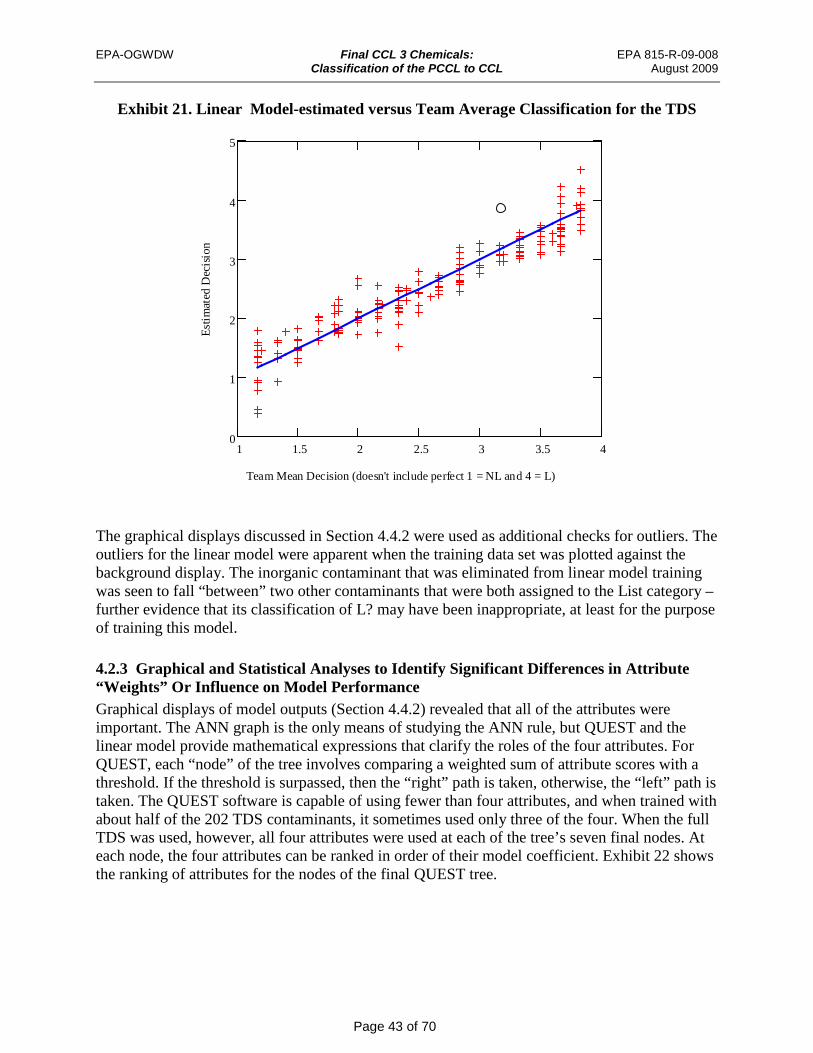
EPA-OGWDW Final CCL 3 Chemicals: EPA 815-R-09-008
Classification of the PCCL to CCL August 2009
Page 43 of 70
Exhibit 21. Linear Model-estimated versus Team Average Classification for the TDS
1 1.5 2 2.5 3 3.5 4 0
1
2
3
4
5
Estim
ated
Dec
isio
n
Team Mean Decision (doesn't include perfect 1 = NL and 4 = L)
The graphical displays discussed in Section 4.4.2 were used as additional checks for outliers. The outliers for the linear model were apparent when the training data set was plotted against the background display. The inorganic contaminant that was eliminated from linear model training was seen to fall “between” two other contaminants that were both assigned to the List category – further evidence that its classification of L? may have been inappropriate, at least for the purpose of training this model. 4.2.3 Graphical and Statistical Analyses to Identify Significant Differences in Attribute “Weights” Or Influence on Model Performance Graphical displays of model outputs (Section 4.4.2) revealed that all of the attributes were important. The ANN graph is the only means of studying the ANN rule, but QUEST and the linear model provide mathematical expressions that clarify the roles of the four attributes. For QUEST, each “node” of the tree involves comparing a weighted sum of attribute scores with a threshold. If the threshold is surpassed, then the “right” path is taken, otherwise, the “left” path is taken. The QUEST software is capable of using fewer than four attributes, and when trained with about half of the 202 TDS contaminants, it sometimes used only three of the four. When the full TDS was used, however, all four attributes were used at each of the tree’s seven final nodes. At each node, the four attributes can be ranked in order of their model coefficient. Exhibit 22 shows the ranking of attributes for the nodes of the final QUEST tree.

EPA-OGWDW Final CCL 3 Chemicals: EPA 815-R-09-008
Classification of the PCCL to CCL August 2009
Page 44 of 70
Exhibit 22. Relative Weights of Attributes at QUEST Nodes (1 = greatest weight, 4 = least weight)
Node # 1 Potency Severity Prevalence Magnitude N 2 1 1 2 4 3 202 2 1 2 4 3 141 3 2 1 3 4 61 4 1 3 4 2 52 5 1 2 4 3 89 7 1 3 4 2 18 28 2 1 3 4 23
1 Numbers as assigned by QUEST. 2 N = Number of TDS contaminants that are evaluated at the node. All 202 are evaluated at the first node. Of
these, 141 proceed to node 2, while the remaining 6 1 pass to node 3 (see Appendix E for additional details).
Overall, it appears that Potency carries the most weight, followed by Severity, Magnitude and, Prevalence.
The linear model assigns a weight to each attribute and the greatest of these is that of Potency, followed by Severity, Prevalence, and Magnitude (see also Appendix E). The order of Prevalence and Magnitude is the reverse of that found for QUEST. The linear model also provides a means of testing the statistical significance of the intercept and four coefficients. Because the model accounts for possible censoring, this testing is not as simple as in a least-squares regression. Two methods were used to approximate the covariance matrix for this model. The first is based on the Fisher information (J(model parameters θ)), derived using the likelihood function, L(data|θ):
J(θ) = - E [d2 ln(L(data|θ)) / dθ2 | θ]
The second used a Bayesian posterior sample of parameter values. This sample produced a covariance matrix that was nearly identical to that derived from the Fisher information, suggesting that the likelihood and posterior are very nearly multivariate normal. Hypothesis tests could therefore be conducted using the Markov Chain Monte Carlo (MCMC) sample (10,000 sets of parameter values). Exhibit 23 below shows means, medians, and 95% credible intervals for the model parameters. b1 through b4 are the parameters for the four attributes (Potency, Severity, Prevalence, and Magnitude, respectively), b0 is an intercept term, and Phi is the precision (inverse of the error variance). The 95% intervals reveal that all of the attribute parameters are statistically significantly greater than zero.

EPA-OGWDW Final CCL 3 Chemicals: EPA 815-R-09-008
Classification of the PCCL to CCL August 2009
Page 45 of 70
Exhibit 23. Summary Statistics from MCMC Sample Parameter Mean 2.5% Median 97.5%
b0 -1.674 -1.865 -1.673 -1.488 b1 0.2410 0.3343 0.241 0.2591 b2 0.2170 0.2002 0.2169 0.2342 b3 0.1157 0.1033 0.1157 0.1284 b4 0.1699 0.1539 0.1699 0.1858 Phi 14.25 11.44 14.22 17.41
Based on the MCMC sample, pair wise comparisons of attribute parameters were all found to be statistically significant. Separate weights are needed for the two health effects attributes and for the two occurrence attributes. 4.3 Model Performance Testing The TDS, Attribute Scoring Protocols, and prototype model test results were linked together in an iterative process. Testing of the models in the early stages was impacted by changes and refinements in attribute scales, resulting changes in the scores, and changes in the composition of the TDS. These changes required iterative reevaluation of the models and resulted in many improvements that are part of this final analysis. Refinements in scoring are discussed further in Chapter 2 and development of the TDS in Chapter 3. EPA also evaluated the impact of the attributes used by the models and the effects of missing data on the performance of the models during the various stages of development. During e arly stages of the model testing, the models were run with various sized TDSs. The CART and MARS models did not always use all four attributes with some of the smaller TDSs. However, all models used all four attributes when trained with the final TDS, consisting of 202 contaminants. Exploratory analysis of the results revealed some additional problems with the CART and MARS models. When two contaminants have identical attribute scores for all but one attribute, the contaminant with the higher score for that attribute should logically be classified at least as high as the contaminant with the lower score. For example, if a contaminant with scores (4, 4, 4, 4) is assigned to the L? Category, then a contaminant with scores (4, 4, 4, 5) should not be assigned lower, to category NL? or NL. Both CART and MARS rules had this type of misclassification. Both models did not consistently classify contaminants. Another problem with the CART and MARS models was their errors across two categories. Both models did not consistently separate the NL? from the L contaminants or separate the L? from the NL contaminants. Because of these problems, and because of poor performance with respect to the training set decisions, EPA decided not to use these two models to inform PCCL to CCL decisions. Three models, ANN, QUEST and Linear Regression consistently demonstrated the best performance when using the final TDS. Exhibit 24 lists the features of these three models.

EPA-OGWDW Final CCL 3 Chemicals: EPA 815-R-09-008
Classification of the PCCL to CCL August 2009
Page 46 of 70
Exhibit 24. Features of the Three Preferred Models Based on TDS Test Results
Features
Classification Models
Artificial Neural Network
Classification Tree with Linear Nodes
(QUEST) Linear Regression
Objective Function Minimize count of Minimize count of Maximize (to be minimized training set errors training set error likelihood or or maximized) loss OR minimize
error loss minimize error loss
Prediction Rounded average subject matter
expert classification
Rounded average subject matter
expert classification
Average subject matter expert
classification (not rounded)
Ranking Rank by Probability Rank by Rank by prediction Capability (Probability of List) classification and
distance from discriminant
(requires postprocessing)
Transparency of Optimization Method
Not transparent Not transparent Simple and transparent
Classification Rule Not clear, but classifications
available for all attribute score
combinations.
Clear. Complex classification tree
with linear inequalities for
intermediate nodes
Clear. Simple linear function of attribute
scores.
Computation < 1 Second < 1 Second (but < 1 Second Speed process for deriving
distances for ranking is not part
of software) Software Cost Version used is
Freeware. Freeware No special software
4.4 Evaluating Classification Differences This section describes how the classification models were assessed and compared with respect to:
• The number of correct and incorrect classifications for the 202 contaminants in the final TDS
• The number of “large” misclassifications (off by more than one category) • The weighted sum of TDS classification errors • Ability to identify intermediate classifications • Consistent behavior (e.g., no decreasing classification as attribute scores increase)
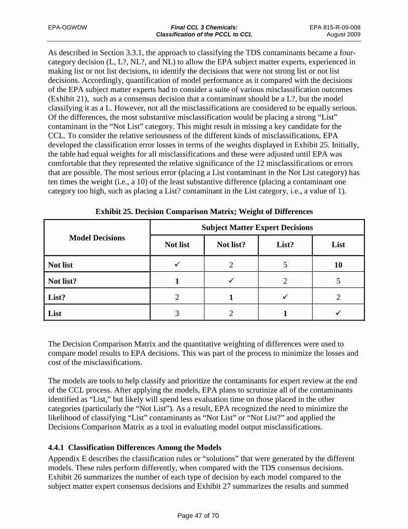
EPA-OGWDW Final CCL 3 Chemicals: EPA 815-R-09-008
Classification of the PCCL to CCL August 2009
Page 47 of 70
As described in Section 3.3.1, the approach to classifying the TDS contaminants became a four-category decision (L, L?, NL?, and NL) to allow the EPA subject matter experts, experienced in making list or not list decisions, to identify the decisions that were not strong list or not list decisions. Accordingly, quantification of model performance as it compared with the decisions of the EPA subject matter experts had to consider a suite of various misclassification outcomes (Exhibit 21), such as a consensus decision that a contaminant should be a L?, but the model classifying it as a L. However, not all the misclassifications are considered to be equally serious. Of the differences, the most substantive misclassification would be placing a strong “ List” contaminant in the “Not List” category. This might result in missing a key candidate for the CCL. To consider the relative seriousness of the different kinds of misclassifications, EPA developed t he classification error losses in terms of the weights displayed in Exhibit 25. Initially, the table had equal weights for all misclassifications and these were adjusted until EPA was comfortable that they represented the relative significance of the 12 misclassifications or errors that are possible. The most serious error (placing a List contaminant in the Not List category) has ten times the weight (i.e., a 10) of the least substantive difference (placing a contaminant one category too high, such as placing a List? contaminant in the List category, i.e., a value of 1).
Exhibit 25. Decision Comparison Matrix; Weight of Differences
Model Decisions Subject Matter Expert Decisions
Not list Not list? List? List
Not list
2
5
10
Not list?
1
2
5
List?
2
1
2
List
3
2
1
The Decision Comparison Matrix and the quantitative weighting of differences were used to compare model results to EPA decisions. This was part of the process to minimize the losses and cost of the misclassifications. The models are tools to help classify and prioritize the contaminants for expert review at the end of the CCL process. After applying the models, EPA plans to scrutinize all of the contaminants identified as “List,” but likely will spend less evaluation time on those placed in the other categories (particularly the “Not List”). As a result, EPA recognized the need to minimize the likelihood of classifying “List” contaminants as “Not List” or “Not List?” and applied the Decisions Comparison Matrix as a tool in evaluating model output misclassifications. 4.4.1 Classification Differences Among the Models Appendix E describes the classification rules or “solutions” that were generated by the different models. These rules perform differently, when compared with the TDS consensus decisions. Exhibit 26 summarizes the number of each type of decision by each model compared to the subject matter expert consensus decisions and Exhibit 27 summarizes the results and s ummed

EPA-OGWDW Final CCL 3 Chemicals: EPA 815-R-09-008
Classification of the PCCL to CCL August 2009
Page 48 of 70
products from the Weighted Loss Value (Exhibit 25). The model input (and output) for ANN, CART, MARS, and QUEST were the integers representing the classes (i.e., 4=L, through 1=NL) while the Linear model estimated the average classification. When a majority of subject matter experts favored one classification for a contaminant, that class was assigned. When the subject matter experts were evenly split (for example, if three assigned a contaminant to 1 (NL) and three assigned it to 2 (NL?)), an agreement was reached to assign the contaminant to the higher of the two categories (2 (NL?) in the case of even split between scenario 1 and 2). In contrast, the Linear model predicted the average classification and was trained using average classifications for the TDS. For example, if three decision makers assigned a contaminant to 1 and three assigned it to 2, the average classification was 1.5.
Exhibit 26. Summary of Quaternary Model Decisions
Decision Category
Number of Decisions in Category by Model Expert
Workgroup Blinded Decision
ANN CART Linear MARS QUEST
4 (L) 42 42 27 27 47 55 3 (L?) 56 55 68 69 38 49
2 (NL?) 65 65 73 69 81 58 1 (NL) 39 40 34 37 36 40 Total 202 202 202 202 202 202
Exhibit 27. Results of 202 Model Classifications and Weighted Misclassifications
Number of Classification Weighted Loss matching Value
TDS ANN 168 52
CART 156 84 Linear 160 72
MARS 160 67 QUEST 174 33
While there are important differences, all the models were able to process the TDS and produce classification rules. All five models produced from 79 percent to 86 percent exact matches with the consensus decisions. Exhibit 28 provides further details on the predicted classifications for each model. Perhaps most important, no model classed any consensus L(4) or L?(3) decision as a NL (1). Only CART classed any L(4) candidates (2%) as NL?(2).
The best performance, by these metrics, was that from the QUEST model, while the lowest performance was by CART. The objective of the QUEST model was to minimize the value loss of the misclassifications, while the other methods minimized errors with no regard for the
EPA-OGWDW Final CCL 3 Chemicals: EPA 815-R-09-008
Classification of the PCCL to CCL August 2009
Page 49 of 70
weights shown in Exhibit 25. As a result, QUEST has the lowest loss, and the highest exact match rate. Note on Exhibit 28, that QUEST’s misclassifications are all shifted to the “left;” i.e., QUEST only predicted 2 of consensus L? decisions would be NL?; and 8 of consensus NL? were predicted to be L?. EPA believes this is a more acceptable and conservative difference. ANN attempts to maximize the likelihood of correct predictions and simply minimize the number of misclassifications (not their weighted value). Its misclassifications are rather equally distributed around the exact match categories. The performance of MARS and the Linear model look similar, but MARS had the highest value of any model for consensus L? decisions that were predicted as NL? (16), a less acceptable difference. 4.4.2 Logical Evaluation of the Models – G raphical Analysis As introduced in Section 3.2.1, the testing of the models included evaluation of the total potential “attribute space.” The total “attribute space” for a model that includes four attributes with scores from 1 to 10, is 10,000 combinations of possible attribute scores. The graphical analysis of model performance looked at how the models generated decisions on the category to which it assigned contaminants (L or NL). When applied across the entire attribute space, the discriminate surfaces that bound the model’s decisions on the category to which it assigned any possible score became apparent. These category boundaries or discriminant surfaces were reviewed for consistency through the graphical analysis. Five models (ANN, QUEST, MARS, CART, and Linear Regression) developed with the 202 TDS produced classification rules that were applied to the 10,000 scores and plotted to evaluate their performance (Exhibits 29 through 32). Exhibit 29 is another example of the graphic tool introduced in Chapter 3, Exhibit 19, to help visualize the multi-dimensional space of the CCL classifications. The graphical analysis shows five elements of the model results, the four attributes evaluated and the categorical decision (L, L?, NL?, and NL) in a single graph. Note in Exhibit 29 that the vertical and horizontal axes show two attributes on each axis. The attribute scores for Potency are the large squares across the horizontal axis. The corresponding score for Severity for each Potency score is a separate scale within each larger square. That is, each Potency square has a range of Severity scores. Similarly the Prevalence and Magnitude scores are plotted on the vertical axis with Prevalence along the primary axis and Magnitude along the axis imbedded in each Prevalence square. The categorical decision assigned to each potential attribute score combination is color coded. Red represents a L decision, beige, a L?; light blue represents a NL? and dark blue represents a NL decision.

EPA-OGWDW Final CCL 3 Chemicals: EPA 815-R-09-008
Classification of the PCCL to CCL August 2009
Page 50 of 70
Exhibit 28. Summary of Individual Quaternary Model Classifications (shaded cells are exact match with Expert Decisions)
Consensus Blinded Model Decisions
Decisions ANN 4 (L) 3 (L?) 2 (NL?) 1 (NL)
4 (L) 37 5 0 0 3 (L?) 5 44 7 0
2 (NL?) 0 6 53 6 1 (NL) 0 0 5 34 CART 4 (L) 3 (L?) 2 (NL?) 1 (NL)
4 (L) 26 12 4 0 3 (L?) 1 47 8 0
2 (NL?) 0 9 53 3 1 (NL) 0 0 8 31 Linear 4 (L) 3 (L?) 2 (NL?) 1 (NL)
4 (L) 26 16 0 0 3 (L?) 1 47 8 0
2 (NL?) 0 6 54 5 1 (NL) 0 0 7 32 MARS 4 (L) 3 (L?) 2 (NL?) 1 (NL)
4 (L) 37 5 0 0 3 (L?) 10 30 16 0
2 (NL?) 0 3 59 3 1 (NL) 0 0 6 33 QUEST 4 (L) 3 (L?) 2 (NL?) 1 (NL)
4 (L) 42 0 0 0 3 (L?) 13 41 2 0
2 (NL?) 0 8 54 3 1 (NL) 0 0 2 37

Exhibit 29. ANN Model Predictions for the Four Attribute Space(10,000 possible score combinations)
EPA-OGWDW Final CCL 3 Chemicals: EPA 815-R-09-008 Classification of the PCCL to CCL August 2009
Page 51 of 70
The colors represent the classification decision: List = red; List? = beige; Not List? = light blue, and Not List = dark blue. One TDS
contaminant (Potency = 4, Severity = 8, Prevalence = 5, and Magnitude = 10) is shown in black, though EPA’s decision for that contaminant is List (red). This particular contaminant is always shown in contrasting color to help the viewer orient to the details of the
graph and check the scaling and axes. ____________________
1 Expressed in R GB format, dark blue is (5 113 176), light blue is (146 197 222), beige is (244 165 130), and red is (202 0 32). These colors were selected using ColorBrewer, by Cynthia A. Brewer of Penn State University. ColorBrewer can be found online at
www.ColorBrewer.org.

EPA-OGWDW Final CCL 3 Chemicals: EPA 815-R-09-008
Classification of the PCCL to CCL August 2009
Page 52 of 70
Exhibit 29 plots the results of the ANN models classifications for the 10,000 combinations of attribute scores. The patterns clearly show a logical progression from the lower left to upper right, progressing from Not list predictions (dark blue) for low attribute scores, through NL? and L?, to List classifications for the highest scores, both within each square and across the entire matrix. The graphical analysis helped to understand and visualize the logic of the discriminant approach of models and to visualize the performance with the TDS. The QUEST model produces a very similar graphic result to the ANN model. In contrast to Exhibit 29, Exhibit 30 shows the MARS results. The figure shows areas where red (L) directly touches light blue (NL?) and where dark blue (NL) touches beige (L?). Both are indications that the model was unable to define the intermediary categories. Another problem can be seen in the lower right box of the figure, where Potency is 10 and Prevalence is 1. Within that box, when magnitude is 1(along the bottom edge of the box), as Severity increases, the decision can be seen to go directly from NL? to NL (light blue to dark blue). This unacceptable result also occurs for several other combinations of high Potency and low Prevalence. EPA found that these results were illogical and unacceptable. Exhibit 31 shows that the univariate CART model exhibited similar problems. The adapted Linear Regression model, shown in Exhibit 32, presents an interesting variant. As noted, the Linear model predicts average classification of contaminants. In other words in contrast to ANN or QUEST which predict a classification as an integer of 3 (or L?), the Linear model predicts the value from the regression model, such as 3.312 (rounded to 3 = L?), so the colors can be displayed more as a continuous variable. The Linear model again displays a very logical function across the total attribute space. As discussed above, the CART and MARS models exhibited inconsistent categorization of contaminants and poor performance in the decision matrix comparisons, while the other three models (ANN, Linear, and QUEST) performed very well with respect to TDS error loss, number of training set errors, and the logic of the classification model. The linear model was generally able to predict EPA average within approximately 0.3 (less than half a category). Hence, evaluating ways to apply the model results focused on procedures for utilizing the results from the ANN, Linear, and QUEST models.

Exhibit 30. MARS Model Predictions for the Four Attribute Space(10,000 possible score combinations).
See Exhibit 29 for the key and text for discussion.
EPA-OGWDW Final CCL 3 Chemicals: EPA 815-R-09-008 Classification of the PCCL to CCL August 2009
Page 53 of 70

EPA-OGWDW Final CCL 3 Chemicals: EPA 815-R-09-008
Classification of the PCCL to CCL August 2009
Page 54 of 70
Exhibit 31. Univariate CART Model Predictions for the Four Attribute Space (10,000 possible score combinations)
See Exhibit 29 for the key and text for discussion.

Exhibit 32. Linear Model Predictions for the Four Attribute Space(10,000 possible score combinations)
See Exhibit 29 for the key and text for discussion.
EPA-OGWDW Final CCL 3 Chemicals: EPA 815-R-09-008 Classification of the PCCL to CCL August 2009
Page 55 of 70

EPA-OGWDW Final CCL 3 Chemicals: EPA 815-R-09-008
Classification of the PCCL to CCL August 2009
Page 56 of 70
4.5 Applying Model Results From the inception of the development of the CCL classification process, EPA intended to use classification models as decision support tools. It was envisioned that, after testing and evaluation, a model(s) might be used to process complex data in a consistent, objective, and reproducible manner and provide a prioritized listing of candidate contaminants for the last stage of the CCL process, an expert review and evaluation. This also would help to focus resources for the review and evaluation of potential contaminants. The use of classification models as a tool in the CCL process is a new application of such tools. Several factors have been considered in assessing how to utilize the model results. After testing, EPA determined that three models performed well: the ANN, Linear, and QUEST models. These are three different classes of models, with three di fferent mathematical approaches, but all provided similar results and logical determinations. Yet the results of each are unique (e.g., Exhibits 29 and 32). Therefore, EPA explored ways to combine the results of all three models, to capture both agreement among models and unique results. Two straight forward approaches looked most useful and were applied: a simple additive approach, and a collective rank-order approach. 4.5.1 Additive Model Results The first step in combining the results of the three models was to simply add the results of their classifications for each contaminant. A tabulation of all contaminants (in the TDS) was prepared with their predicted classification from the models. Recall, the model output is as a class (number), with 4 equaling L through 1 equaling NL. The Linear model output was rounded to its integer class for this approach). Then the 3 results were simply added. This resulted in 10 “bins” or classes, ranging from 3 (all three models classed the contaminant as a 1) to 12 (all three models classed the contaminant as a 4). Hence, a contaminant with an additive score of 11, had two models class it as 4 and one model class it as a 3, totaling 11. A comparison of the sum of the three models to the TDS workgroup Decisions is shown i n Exhibit 33. Exhibit 33, shows some important features of the additive process. For 142 of the 202 contaminants, the three models were unanimous and in agreement with the TDS. When reviewing these analyses EPA noted that every contaminant subject matter experts classed as List (by consensus) was predicted as a List by at least one model. The models do move some NL? into a strong L ? position, but only 2 of the L? contaminants were placed into the NL? category. The areas where the models differ in outcome can provide a place to focus some review during the development of future CCLs. 4.5.2 Additive Rank Order Results EPA also tested a different approach from the 10 additive classes. A simple method to provide a more continuous rank-order for each model was also developed. The output for each model was used to produce a rank-ordering f or that model; ordering f rom highest (an L candidate) as number one, to lowest (a NL) as number 202 for the TDS. Once the ranks for a model were ordered, the contaminants were simply assigned a number from 1 to 202 (high to low). After this was done for all three models, the rank numbers were added (resulting in a range from 3 to 606) divided by 3 (just to stay on the 202 scale), and then reordered by their composite ranks.
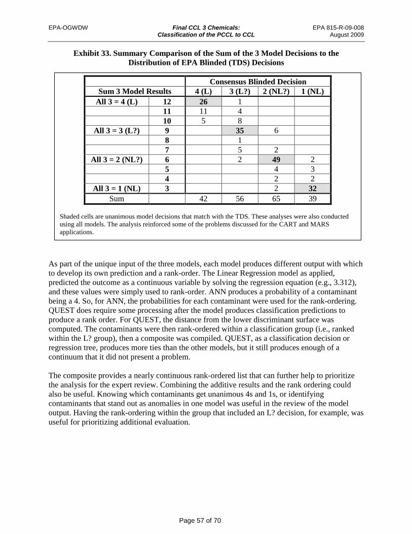
EPA-OGWDW Final CCL 3 Chemicals: EPA 815-R-09-008
Classification of the PCCL to CCL August 2009
Page 57 of 70
Exhibit 33. Summary Compari Distribution of
Sum 3 Model Results
All 3 = 4 (L) 12 11 10
All 3 = 3 (L?) 9 8 7
All 3 = 2 (NL?) 6 5 4
All 3 = 1 (NL) 3 Sum
son of the Sum of the 3 Model Decisions to the EPA Blinded (TDS) Decisions
Consensus Blinded Decision 4 (L) 3 (L?) 2 (NL?) 1 (NL)
26 1 11 4 5 8 35 6 1 5 2 2 49 2 4 3 2 2 2 32 42 56 65 39
Shaded cells are unanimous model decisions using all models. The analysis reinforced som
applications.
that match with the TDS. These analyses were also conducted e of the problems discussed for the CART and MARS
As part of the unique input of the three models, each model produces different output with which to develop its own prediction and a rank-order. The Linear Regression model as applied, predicted the outcome as a continuous variable by solving the regression equation (e.g., 3.312), and these values were simply used to rank-order. ANN produces a probability of a contaminant being a 4. So, for ANN, the probabilities for each contaminant were used for the rank-ordering. QUEST does require some processing after the model produces classification predictions to produce a rank order. For QUEST, the distance from the lower discriminant surface was computed. The contaminants were then rank-ordered within a classification group (i.e., ranked within the L? group), then a composite was compiled. QUEST, as a classification decision or regression tree, produces more ties than the other models, but it still produces enough of a continuum that it did not present a problem.
The composite provides a nearly continuous rank-ordered list that can further help to prioritize the analysis for the expert review. Combining the additive results and the rank ordering could also be useful. Knowing which contaminants get unanimous 4s and 1s, or identifying contaminants that stand out as anomalies in one model was useful in the review of the model output. Having the rank-ordering within the group that included an L? decision, for example, was useful for prioritizing additional evaluation.

EPA-OGWDW Final CCL 3 Chemicals: EPA 815-R-09-008
Classification of the PCCL to CCL August 2009
Page 58 of 70
5.0 MODEL OUTCOME AND POST MODEL EVALUATION PROCESS The preceding chapters have described the process that was developed for selecting the CCL from the PCCL. The companion document, Final CCL 3 C hemicals: Screening to a PCCL (USEPA, 2009b), describes the approach that was used for screening and selecting the PCCL from the Universe of chemicals. Once the PCCL screening was executed, the Attribute Scoring Protocols finalized, and the models trained, all of the PCCL chemicals were scored for their attributes and run through the models. This chapter describes the results from the modeling and the processes EPA used in evaluating the model output before selecting the CCL 3. EPA evaluated the model output and formulated s everal post-model refinements that were added to the CCL selection process, including a n approach for considering the certainty reflected in the differing data elements. The post-model analyses are also described in this Chapter. 5.1 PCCL Characterization and Model Results The screening process, described in “Final CCL 3 Chemicals: Screening to a PCCL” (USEPA, 2009b), selected the chemicals for the PCCL. The attributes for these chemicals were scored using the procedures presented in Chapter 2 and evaluated by the three models described in Chapter 4. Exhibit 34 illustrates the results of the model output for the PCCL contaminants developed for the Draft CCL 3. These results show the distribution of the different types of data and information EPA used to evaluate occurrence and potential occurrence8. The PCCL consisted of chemicals with variable health effects data, ranging from RfDs to LD50, and occurrence data, ranging from measured water concentration data from PWSs to production volume data.
Exhibit 34. Model Results for the PCCL Chemicals
3 Models
Decision
% of PCCL
Total #
PCCL
Finished or
Ambient Water
Release Production
L 9% 44 3 24 17 L-L? 12% 58 9 29 20 L? 33% 163 26 64 73 NL?-L? 6% 30 6 11 13 NL? 28% 139 29 28 82 NL?-NL 4% 20 7 9 4 NL 9% 46 21 7 18 N(all) 100% 500 101 172 227
As described in Chapter 4, three models (ANN, Quest, and Linear) were used in classifying the PCCL contaminants. EPA used an additive process to combine the results of all three models.
8 The screening of the CCL 3 Universe, including processing with supplemental data during the nominations process, resulted in 532 chemical contaminants for the PCCL. These chemicals were scrutinized as part of the classification and modeling process. Some of the PCCL chemicals had limited data available for scoring and could not be run through the models process. The 32 contaminants that had limited data remain on the PCCL. They are identified in Appendix G. Exhibit 34 recaps the model output for the 500 chemicals that were scored and processed.

EPA-OGWDW Final CCL 3 Chemicals: EPA 815-R-09-008
Classification of the PCCL to CCL August 2009
Page 59 of 70
The bolded decision category (i.e. L, L?, NL?, NL) in Exhibit 34 signifies that all of the models were in 100% agreement with that listing decision. The other categories (e.g., NL?-NL) represent varied agreement where one or two of the models choose one listing option and one or two models chose a different option. None of the models categorized a contaminant in a category more than one category higher or lower than the other models. That is, no contaminants were categorized as an “L” by one model and as an “NL?” by another model, or vice versa. The models categorized approximately ½ of the chemicals on the PCCL as L? or above. When analyzed by data type, the majority of chemicals in the List category had LD50 data for health effects. This was a concern and became an important issue for consideration in the post-model evaluation process. 5.2 Evaluation of the Modeling Output As part of the last stage in the CCL classification process, the model output was reviewed by internal EPA experts. This step involved:
• a more detailed review of the data used, • a review of supplemental data, and • deliberations on how the model data should be used to produce a draft proposal for a
CCL. Specifically, the function of the team was to critically compare the results from the model to the information collected for the individual chemicals, and identify any concerns with the model output. This exercise was conducted for a cross section of the model outcomes and their associated contaminants. An Evaluation Team was comprised of internal EPA experts representing scientists, engineers, toxicologists, and environmental protection specialists from the OW, Office of Research and Development, Office of Children’s Health, and Office of Pesticide Programs. The Evaluation Team met on a weekly basis for approximately 8 weeks to discuss the evaluation of modeling results. 5.2.1 Procedure Prior to the initiation of the evaluation effort, all Evaluation Team members received background descriptions of the CCL process for chemicals (Chapters 1-4 of this document), Attribute Scoring Protocols, and evaluation work sheets. A spread sheet with the attribute scores, the data that supported the scores, and the model output for each of the chemicals selected for the first review session was also included in the package. An initiation meeting was held to familiarize the participants with the contents of their evaluation package and discuss the approach that would be followed in evaluating the model output for individual contaminants. Participants on the Evaluation Team received a set of contaminants and supplemental data dossiers for evaluation. The completed evaluation sheets were submitted so that the results could be compiled for discussion. The evaluation sheets allowed the participants to:

EPA-OGWDW Final CCL 3 Chemicals: EPA 815-R-09-008
Classification of the PCCL to CCL August 2009
• Comment on the model input data for each attribute, • Provide a statement on their level of confidence in the data underlying each attribute
score, • Express agreement or disagreement with the model output, • Indicate their degree of confidence in the model decision, and • Provide an explanation for their agreement of lack of agreement with the model decision.
Following submission of the evaluation results for each set of contaminants, the Evaluation Team discussed the outcome of the evaluation, concentrating first on those contaminants with the greatest differences among the reviewers. These discussions identified the issues and steps described in the following sections of this chapter. The Evaluation team reviewed a subset of 129 chemicals from the PCCL. The contaminants were divided into groups as follows: • Contaminants with finished and/or ambient water data, • Contaminants with release data (pesticide applications and/or TRI), and • Contaminants with production data. The team evaluated all contaminants with finished and/or ambient water data and a randomly chosen subset of the contaminants with release or production data. The identities of the contaminants were blinded for the review. This was done so that the team would focus their review on the data for a contaminant and not its name. The identity of all contaminants was revealed when the team discussed the evaluation results. 5.2.2 Evaluation Results Discussion of the model results raised issues that are important to the selection process for CCL 3 a nd subsequent CCLs. The evaluators represented a variety of disciplines and contributed important perspectives reflecting their field of specialization. Below are some of the important issues that were raised by evaluators:
• The ratio between the health reference value and the concentrations observed in finished
and/or ambient water is an important relationship that is not entirely captured by the four attribute scores. When finished and/or ambient water data were available, this ratio was most often the reason for not agreeing with the model output. For example, the model may have classified a chemical as an L?, but when the health value and concentration data were directly compared, the outcome indicated that occurrence was one or more orders of magnitude below the health-based benchmark. In this situation, the evaluators usually disagreed with the models decision.
• Confidence in the data elements used for attribute scoring varied widely among the
PCCL contaminants. Evaluators noted that there was a considerable difference in the weight-of-evidence for the differing types of data used to score PCCL contaminants. Although the scores used a hierarchy in selecting the data elements that best represented health effects and occurrence, the most highly ranked data element was not equivalent for every chemical. Individual chemicals used different combinations of data as input for the models. The type of data elements used to represent the occurrence and health effects
Page 60 of 70

EPA-OGWDW Final CCL 3 Chemicals: EPA 815-R-09-008
Classification of the PCCL to CCL August 2009
Page 61 of 70
became a subject of discussion for the Evaluation Team. Some contaminants had recent UCMR monitoring data combined with an Office of Pesticide Programs (OPP) RfD and others had TRI release data combined with an LD50. For some chemicals, the only available data came from an LD50 combined with the number of pounds produced per year and environmental fate properties. The evaluators were more comfortable with the model decisions based on strong supporting data (i.e., RfD and finished water occurrence) than on those based on weak data sets (i.e., LD50 and production data).
• Reviewers believed it was important that the occurrence and health values represent the
same form of the chemical. This is particularly important for nonmetals where the common inorganic form of the element is a complex ion (i.e. phosphate) and not the element (i.e. phosphorous). This is also important for metals (i.e vanadium) where the occurrence data represent ions in solution that may have been paired with a toxicity value for the free metal.
• Toxicity data from National Cancer Institute/National Toxicity Program bioassays were
incorporated into the Universe for a number of contaminants that were positive for tumors, and were tested by way of the inhalation route of exposure. Some of these contaminants were screened to the PCCL on the basis of their qualitative cancer findings. They were scored for Potency and Severity based on slope factors that had been derived for the oral route of exposure, but based on the inhalation data without the use of Physiologically Based Pharmacokinetic (PBPK) modeling. Some of these very volatile contaminants received L or L? model designations. Reviewers questioned whether toxicity data from inhalation studies should be used for scoring cancer Potency. Therefore, only cancer slope factors that were derived using PBPK modeling for cross route extrapolation were used to score chemicals. Inhalation data were not used for non-cancer endpoints.
• Due to the risk assessment policy differences between agencies, the hierarchy for scoring
Potency and Severity considered the agency that established the value (described in Chapter 2 and listed in Appendix A). However, some reviewers questioned whether the date of the assessment rather than the Agency conducting the assessment should be the basis for the hierarchy.
• Prevalence and Magnitude were given the lowest possible scores (“1”) when a
contaminant had been monitored but there were no detections. Since the detection level for a few chemicals was above the health-based value, some reviewers questioned whether this was appropriate. They suggested that it might be better to use the detection limit as the basis of the Magnitude a ttribute score.
• UCMR 1 screening studies monitored a small number of statistically selected sites (300).
There were cases where there were no finished water detections in the screening surveys, but the same contaminant had been detected in ambient water by USGS. Reviewers questioned the placement of finished water above ambient water in the hierarchy in these cases.
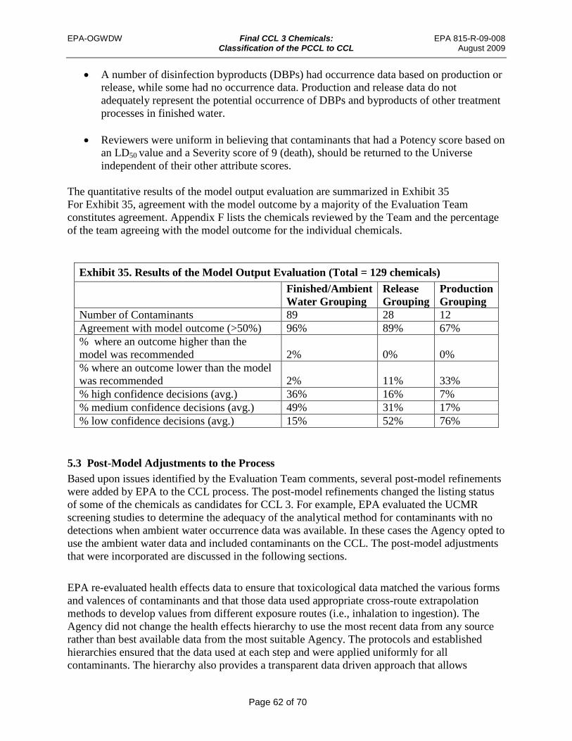
EPA-OGWDW Final CCL 3 Chemicals: EPA 815-R-09-008
Classification of the PCCL to CCL August 2009
Page 62 of 70
Exhibit 35. Results of the Model Output Evaluation (Total = 129 chemicals)
Finished/Ambient Water Grouping
Release Grouping
Production Grouping
Number of Contaminants 89 28 12 Agreement with model outcome (>50%) 96% 89% 67%
% where an outcome higher than the model was recommended
2%
0%
0%
% where an outcome lower than the model was recommended 2% 11% 33% % high confidence decisions (avg.) 36% 16% 7% % medium confidence decisions (avg.) 49% 31% 17% % low confidence decisions (avg.) 15% 52% 76%
• A number of disinfection byproducts (DBPs) had occurrence data based on production or release, while some had no occurrence data. Production and release data do not adequately represent the potential occurrence of DBPs and byproducts of other treatment processes in finished water.
• Reviewers were uniform in believing that contaminants that had a Potency score based on
an LD50 value and a Severity score of 9 (death), should be returned to the Universe independent of their other attribute scores.
The quantitative results of the model output evaluation are summarized in Exhibit 35 For Exhibit 35, agreement with the model outcome by a majority of the Evaluation Team constitutes agreement. Appendix F lists the chemicals reviewed by the Team and the percentage of the team agreeing with the model outcome for the individual chemicals.
5.3 Post-Model Adjustments to the Process Based upon issues identified by the Evaluation Team comments, several post-model refinements were added by EPA to the CCL process. The post-model refinements changed the listing status of some of the chemicals as candidates for CCL 3. For example, EPA evaluated the UCMR screening studies to determine the adequacy of the analytical method for contaminants with no detections when ambient water occurrence data was available. In these cases the Agency opted to use the ambient water data and included contaminants on the CCL. The post-model adjustments that were incorporated are discussed in the following sections.
EPA re-evaluated health effects data to ensure that toxicological data matched the various forms and valences of contaminants and that those data used appropriate cross-route extrapolation methods to develop values from different exposure routes (i.e., inhalation to ingestion). The Agency did not change the health effects hierarchy to use the most recent data from any source rather than best available data from the most suitable Agency. The protocols and established hierarchies ensured that the data used at each step and were applied uniformly for all contaminants. The hierarchy also provides a transparent data driven approach that allows
EPA-OGWDW Final CCL 3 Chemicals: EPA 815-R-09-008
Classification of the PCCL to CCL August 2009
Page 63 of 70
stakeholders and the public to uniformly understand the assumptions and processes that were applied in the selection of data for individual contaminants.
Issues raised by the Evaluation Team may have been addressed by one of the post-model adjustments and processes. For example, several of the scoring or hierarchical issues identified were addressed by implementing the Health-Concentration Ratio. This process addressed concerns about the occurrence data hierarchy, magnitude scores based on detection rather than the method reporting limit, and using the most relevant data to make listing decisions. 5.3.1 Using Supplemental Sources to Identify the Data Most Relevant to Drinking Water One issue identified by the Evaluation Team was that scoring should be based on the data most relevant to exposure from drinking water. For example, DBPs were included in the Universe and many were brought forward to the PCCL. The data used to score these contaminants for occurrence should be based on their occurrence in drinking water at PWSs, not ancillary data that may be available such as release or production volume. There are DBP data from the Information Collection Rule monitoring and supplemental studies identified in the CCL Nominations process. These data had not originally been included in the data used for scoring Prevalence and Magnitude. As part of the post-model processing EPA retrieved the data, scored the chemicals, and ran the models using the supplemental data 5.3.2 Calculation of a Health Effect-Concentration Ratio for Contaminants with Water Data The models classified chemicals using scores for the four attributes. The Evaluation Team recognized that the relationship between Potency and Magnitude was important when deciding whether or not to list a chemical. Therefore EPA calculated the ratio between the health-based value and the 90th percentile concentration in finished or ambient water as a post-model process to select contaminants for the CCL 3. EPA also sought models to predict water concentrations for contaminants that did not have direct measurements in water sources to calculate this ratio. EPA used the health effect-concentration ratio as key criterion for listing a contaminant on the CCL 3if this value was less than or equal to 10. 5.3.2.1 Developing a Health Reference Level (HRL) To calculate the health effect-concentration ratio, the data that provided the Potency score were used to calculate the HRL benchmark using a process similar to the one the Agency has used for Regulatory Determination. For a carcinogen, the HRL is the one-in-a-million cancer risk expressed as a drinking water concentration. For non-carcinogens, the HRL is equivalent to the lifetime health advisory value. The lifetime health advisory value is obtained by multiplying the RfD times 70 kg, dividing by a water intake of 2 L/day and multiplying by a 20% relative source contribution (unless there are data to suggest that the 20% is inappropriate). Determining the HRL for chemicals where the Potency value was the NOAEL, LOAEL, or LD50 value from an individual study, required application of an uncertainty factor to adjust the toxicity value to an RfD approximation. In these cases, the uncertainty factor was based on the difference

EPA-OGWDW Final CCL 3 Chemicals: EPA 815-R-09-008
Classification of the PCCL to CCL August 2009
Page 64 of 70
in the modal values from the log-based data distributions used to develop the Potency scoring equations (see Chapter 2). The uncertainty factors applied are as follows:
• NOAEL = 1,000 • LOAEL = 3,000 • LD50 = 100,000
The NOAEL and LD50 uncertainties were derived from the difference in the constant for the non-cancer Potency scoring e quation (Exhibit 4). For a NOAEL, the difference is 3 (7 – 4 = 3) or 1,000 since the Potency equation is log based. The difference for an LD50 is 5 (7-2 = 5) or 100,000. The uncertainty factor (3,000) chosen for the LOAEL is a half log g reater than that for the NOAEL, in recognition that the LOAEL is a level that causes effects rather than no effects. Exhibit 36 shows the formulae used (including the uncertainty factors), for the CCL 3 pr ogram, to calculate HRLs from the various Potency data elements. The formulae calculate the HRL as a mg/L equivalent, in turn the HRL was converted to μg/L to compare with the CCL 3 water data.
Exhibit 36. Formulae used in the CCL 3 Process to Calculate Health Reference Levels (HRLs) from the CCL 3 Potency Data Elements. The formulae identify the uncertainty factors (UF) applied for the CCL 3. The HRLs are in mg/L. They were further converted to ug/L for comparison with CCL 3 water data. BW = body weight; RSC = relative source contribution.
Non-Cancer Equations
HRL, mg/L = RfD (mg/kg/day) x BW (70 kg ) x RSC (0.2) 2 L/day
HRL, mg/L = NOAEL (mg/kg/day) x BW (70 kg ) x RSC (0.2) 2 L/day x UF (1,000)
HRL, mg/L = LOAEL (mg/kg/day) x BW (70 kg ) x RSC (0.2) 2 L/day x UF (3,000)
HRL, mg/L = LD50 (mg/kg) ) x BW (70 kg ) x RSC (0.2) 2 L/day x UF (100,000)
Cancer Equations
HRL, mg/L = Risk (10-6) x BW (70 kg) Slope Factor x 2 L/day
HRL, mg/L = 10-4 Cancer Risk (mg/L) x 0.01

EPA-OGWDW Final CCL 3 Chemicals: EPA 815-R-09-008
Classification of the PCCL to CCL August 2009
Page 65 of 70
5.3.2.2 Developing a HRL – Concentration Ratio EPA determined that if the measured or modeled concentration of contaminants was equal to or greater than on tenth of the health reference l evel then the contaminant should be included on the CCL 3. EPA selected the 90th percentile (of detections) water concentration as the point of comparison for the ratio, rather than the mean or median. The CCL list is designed to identify contaminants that may benefit from a Health Advisory, even if they do not merit a positive regulatory determination. The 90th percentile concentration level was used as a public health protective benchmark that may identify a possible need for a health advisory for areas of the country that may have higher concentrations in drinking water than others. If a 90th percentile concentration level was not available the Agency used the maximum or the next highest percentile (i.e., 95th or 99th percentile) reported value. The ratio of the heath-value to the 90th percentile concentration detected in water (either ambient or finished) was calculated for all contaminants with water data. If the ratio was 10 or less the contaminant was selected for consideration for the CCL 3. If the ratio was greater than 10, the contaminant was eliminated from consideration for CCL 3 a nd remains on the PCCL. For chemicals that had been monitored but not detected, and for chemicals that were detected in ambient waters but not finished water, analytical method detection limits were compared to the HRL to ensure that the detection accounted for the health effects. Consideration was also given to whether the ambient water data suggested that the UCMR 1 screening might have been too limited to identify the contaminant in areas where it might pose a problem. For contaminants that had limited finished water data, but more robust ambient water monitoring da ta, the ambient water concentration was used to develop the ratio. The contaminant information sheets note which data were used to develop the ratio and are available for all PCCL contaminants in the docket at www.regulations.gov. 5.3.2.3 Developing a Ratio for Contaminants Without Concentration Data EPA used modeled data for pesticides when concentration data were not available. The modeled concentrations of pesticides in water are included in the OPP registration and re-registration evaluation documentation, but they are not readily available in a form that could be used for the Universe database. The modeled data predicts environmental concentrations in ground water and surface water using a standardized approach for pesticides. For pesticides, the modeled data from OPP were compared with the health reference level. As part of the pesticide registration process, EPA calculates an estimated environmental concentration (EEC) in water or estimated drinking water concentration (EDWC) depending on the year the last assessment was completed. Both the EEC and EDWC are derived from models that estimate the pesticide's concentration in an index reservoir used for drinking water. OPP used the PRZM-EXAMS model for surface water. Ground water concentrations are derived using the SCI-GROW regression model to represent exposures in shallow ground water. Both the EEC and the EDWC are equivalent. The modeled EEC values allowed EPA to calculate the HRL/EEC or EDWC ratio for pesticides and/or their degradates. Pesticides with HRL/EEC ratios of 10 and lower were selected for the draft CCL 3.

EPA-OGWDW Final CCL 3 Chemicals: EPA 815-R-09-008
Classification of the PCCL to CCL August 2009
Page 66 of 70
5.3.3 Grouping Contaminants based on the Certainty or Relevance of the Supporting Data Data certainty was not directly factored into the development of the attribute scoring protocols, but was indirectly factored into the protocols through the use of the hierarchies of the data used for health effects and occurrence (Chapter 2). In the evaluation of the model output, data certainty was an important factor for the Evaluation Team. In cases where the model output listed a chemical with well developed data from high in the hierarchy (e.g. IRIS RfD, UCMR/NAWQA concentration), the Evaluation Team typically agreed with the model decision. The Evaluation Team confidence ranking for model decisions based on these types of data was generally high while confidence for less developed or preliminary data from the hierarchy was generally lower (see Exhibit 35). Accordingly, as part of the post-model evaluation process, EPA tried various approaches for addressing the certainty issue. Initially, EPA attempted to develop numeric certainty scores for each data element, but decided not to use this approach because the certainty scores could not be calibrated due to the subjectivity in assigning the numeric values. For example, it would be difficult to justify that a chemical evaluated by environmental release data should be assigned a certainty score of 6, while a chemical evaluated by production volume should be assigned a certainty score of 10 versus 9. Therefore, EPA placed tags on the chemicals that characterize the certainty. The chemicals were tagged as high, medium and low certainty based on the combinations of data elements that were used to score the attributes for health effects and occurrence. The certainty tags are not calibrated measures of certainty. They were developed to express the relative certainty associated with the data elements that were used to score a chemical’s attributes. The certainty rankings assigned to the combinations of individual attribute data elements are listed below:
High Certainty: Finished Water + RfD/ CSF, NOAEL or LOAEL Ambient Water + RfD/CSF, NOAEL Medium Certainty: Ambient Water + LOAEL Release/Application + RfD, NOAEL, LOAEL Production + RfD
Low Certainty: Health effects based on LD50 Occurrence based on production values
The high certainty bin consisted of chemicals that had been scored based on the most relevant data for occurrence in water and with the richest data for health effects. Such contaminants are expected to be good candidates for regulatory determination with minimal research needs. Examples of chemicals in the high bin include chemicals with reference doses and measured water concentration data. The medium bin consists of chemicals that need further occurrence and/or health effects research. These include chemicals that may have well studied health effects data but may need additional occurrence data (e.g. chemicals with release data but, no measured water occurrence data). The low certainty bin consists of chemicals that need extensive health

EPA-OGWDW Final CCL 3 Chemicals: EPA 815-R-09-008
Classification of the PCCL to CCL August 2009
Page 67 of 70
effects and occurrence research needs that may take longer than the life cycle of a CCL. Examples include chemicals with LD50 and/or production volume data. While the CCL consists both of chemicals that may provide sufficient data to support regulatory determinations and chemicals that are of concern and need additional drinking water research EPA found that LD50 and production volume data are not sufficient data for a contaminant to be included on the CCL. EPA evaluated contaminants from each bin to determine if the best available data for that contaminant was sufficient for listing. 5.3.4 LD50 Values with Limited Documentation Following the advice from the Evaluation Team, Severity scores based on death from LD50 studies were subject to additional research to identify supplemental health effects information. If no ot her information were available the contaminants were removed from the modeled PCCL results. (This decision applies to contaminants where no critical endpoint other than death was specified in the source of the LD50 data.) These contaminants were removed from consideration for the CCL. None of the chemicals on the PCCL with LD50 derived health attributes scores had ambient or finished water data. 5.4 Selecting the Draft CCL 3 The chemicals for the draft CCL 3 were selected based on the processes previously described in this document and the other cited support documents, the Final CCL 3 Chemicals: Identifying the Universe (EPA, 2009a), and the Final CCL 3 C hemicals: Screening to a PCCL (EPA, 2009b). The Agency noted from which of the three uncertainty bins, described in Section 5.3.3, contaminants were selected. In selecting c ontaminants for the draft CCL 3, EPA used the post model criteria (described in Section 5.3) for the HRL/Concentration ratio and the certainty bins. EPA identified four groups of on the draft CCL 3.
• 36 chemicals in the high certainty bin, which have finished water data and an HRL/concentration ratio of ≤ 10.
• 24 pesticides in the medium certainty bin, which have modeled surface and/or ground water data that yielded a HRL/concentration ratio of ≤ 10
• 27 pesticides and chemicals in the medium certainty bin, which have release data that gave modeled L or L? rankings
• 8 chemicals were initially in the low certainty bin. These contaminants were nominated and evaluated with supplemental information that was submitted or evaluated by EPA.
No chemicals with only LD50 and production data were selected for the CCL. These chemicals will be considered for future CCLs. Subsequent to placement on the draft CCL 3, the list was subject to review by a panel of qualified external experts and stakeholders. Stakeholder input was considered in determining which chemicals from among a preliminary CCL 3 g rouping were retained for the Draft CCL 3. A summary of this review is available in the docket at www.regulations.gov. The draft CCL 3 was published on February 21, 2008, and included 93 chemicals or chemical groups and 11 microbiological contaminants.
EPA-OGWDW Final CCL 3 Chemicals: EPA 815-R-09-008
Classification of the PCCL to CCL August 2009
Page 68 of 70
5.5 Selecting the Final CCL3
EPA provided information on the process, the draft list, a nd sought comment on its efforts to expand and strengthen the underlying CCL listing process, the draft list, and EPA's efforts to improve the contaminant selection process for future CCLs.
EPA received comments from 177 individuals or organizations on the draft CCL 3. Commenters identified several issues on the draft CCL 3 and the process used to select contaminants for the list. Commenters also provided information and recommendations for the Agency to consider as it finalized the CCL 3. The Agency has provided responses to individual comments in the “Comment Response Document for the Third Drinking Water Contaminant Candidate List (Categorized Public Comments)” document that is available in the regulatory docket at www.regulations.gov (USEPA 2009c).
The EPA SAB and its Drinking Water Committee also reviewed the draft CCL 3 dur ing 2008, and provided an advisory to the EPA Administrator on January 29, 2009. EPA staff met with the SAB to provide an overview of the draft CCL 3, to answer questions from the Drinking Water Committee, and to clarify questions from the full SAB. The Agency also participated in teleconferences with SAB during the development of the “SAB Advisory on EPA's Draft Third Drinking Water Contaminant Candidate List (CCL 3)” (USEPA 2009e).
EPA evaluated all the data and information on chemical contaminants provided by commenters and collected by the Agency after the draft CCL 3 was published. EPA used the same process described in the draft CCL 3 not ice (73 FR 9628, USEPA 2008) and other supporting documents to evaluate contaminants for which data became available after the publication of the draft CCL 3.
The Agency added contaminants to the Universe, adjusted the contaminants that passed through to the PCCL based on new data and reevaluated the PCCL using the protocols described in this document.
The 106 c hemicals included on the final CCL 3 i ncluded:
• 38 chemicals in the high certainty bin • 23 pesticides chemicals in the medium certainty with modeled occurrence data with an
HRL/concentration ratio ≤ 10 • 26 pe sticides and chemicals in the medium bin which have application or release data and
health effects data that resulted in a L, L-L?, or L? classification. • 19 chemicals that were initially in the low or medium certainty bin which EPA or
commenters identified supplementary data that resulted in an HRL/concentration ratio or model classification to be included on the final CCL 3.
5.6 Summary The CCL 3 a nd the process EPA used to select contaminants was developed and tested by the Agency to meet the Safe Drinking Water Act requirements and address recommendations and

EPA-OGWDW Final CCL 3 Chemicals: EPA 815-R-09-008
Classification of the PCCL to CCL August 2009
Page 69 of 70
advice from the NRC (2001) and NDWAC (2004). The Agency has developed a process and final CCL 3 that:
• Considers of a broad Universe of contaminants • Relies on best available science and information to inform the process • Evaluates the known or potential health effects and occurrence in screening the
Universe to a PCCL • Uses a set of contaminant attributes and prototype classification algorithms as decision
support tools in selecting candidates for the CCL from the PCCL • Provides an opportunity for nominations and expert judgment.
The first application of the CCL 3 process accomplished many of the specific recommendations from NRC and NDWAC. During the development of CCL 3, the Agency identified areas for improvement that can be implemented in the selection of CCL 4 and later CCLs.
6.0 REFERENCES Fetter, C. W. 1994. Applied Hydrogeology, 3rd Edition, Macmillan College Publishing Co. New
York.
Lyman, W. J., Reehl, W. F., and Rosenblatt, D. H. 1990. Handbook of Chemical Property Estimation Methods, American Chemical Society, Washington, DC.
National Drinking Water Advisory Council (NDWAC). 2004. National Drinking Water Advisory Council Report on the CCL Classification Process to the U. S. Environmental Protection Agency, May 19, 2004.
National Research Council (NRC). 2001. Classifying Drinking Water Contaminants for Regulatory Consideration. National Academy Press, Washington DC.
NIST. 2006. NIST/SEMATECH e-Handbook of Statistical Methods. Available on the internet at: http://www.itl.nist.gov/div898/handbook/, (used on May 3, 2007).
USEPA. 2004. Office for Water. Drinking Water Standards and Health Advisories, EPA 822-R04-005 Washington, DC. Winter 2004.
USEPA. 2008. Drinking W ater Contaminant Candidate List 3 – Draft Notice. Federal Register. Vol. 72. No. 35. p.9628. February 21, 2008.
USEPA. 2009a. Final Contaminant Candidate List 3 Chemicals: Identifying the Universe. EPA 815-R-09-006. August 2009.
USEPA. 2009b. Final Contaminant Candidate List 3 Chemicals: Screening t o a PCCL. EPA 815R-09-007. August 2009.
USEPA. 2009c. Final Comment Response Document for the Third Drinking Water Contaminant Candidate List (Categorized Public Comments). EPA 815-R-09-010. August 2009.
USEPA. 2009d. Summary of Nominations for the Third Contaminant Candidate List. EPA-815R-09-011. August 2009.
USEPA. 2009e. SAB Advisory on EPA’s Draft Third Drinking Water Contaminant Candidate List (CCL 3). EPA-SAB-09-011. January 2009.

EPA-OGWDW Final CCL 3 Chemicals: EPA 815-R-09-008 Classification of the PCCL to CCL August 2009
Page 70 of 70
7.0 APPENDICES
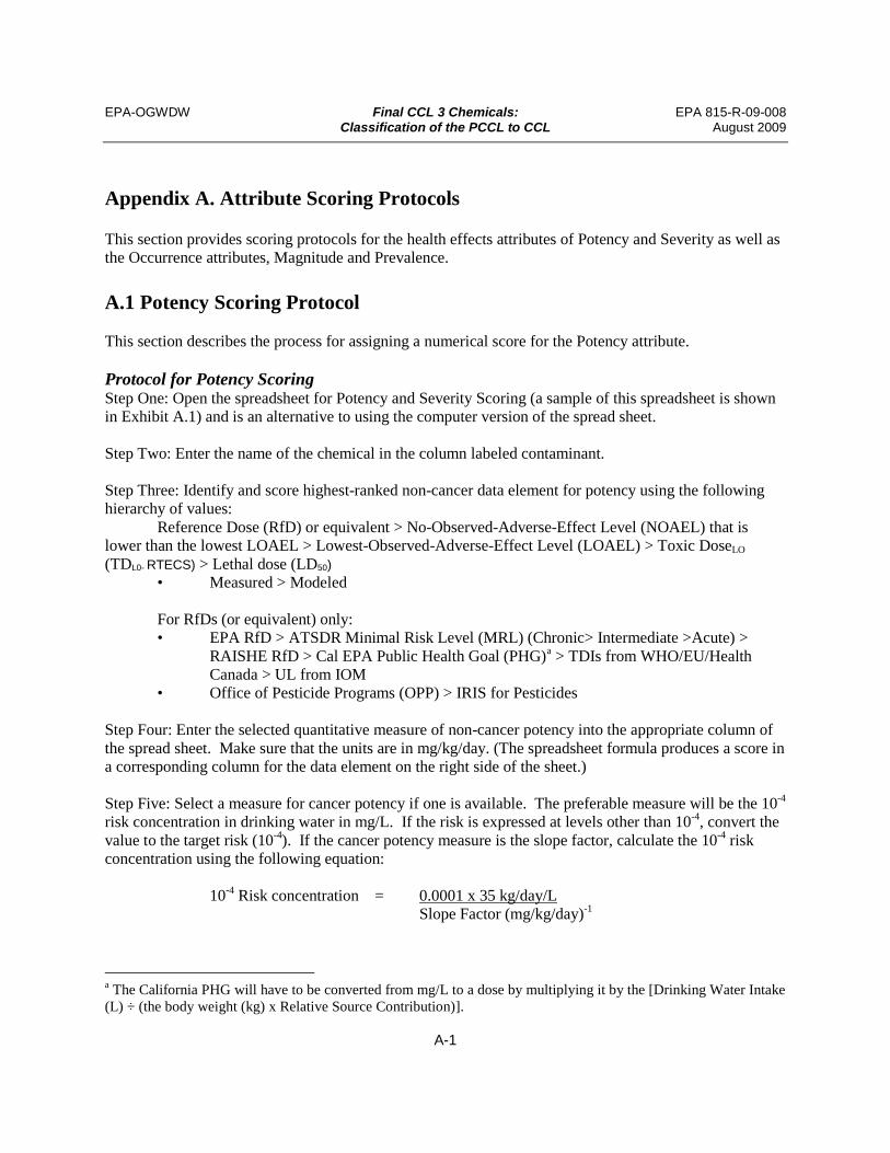
EPA-OGWDW Final CCL 3 Chemicals: EPA 815-R-09-008 Classification of the PCCL to CCL August 2009
Appendix A. Attribute Scoring Protocols This section provides scoring protocols for the health effects attributes of Potency and Severity as well as the Occurrence attributes, Magnitude and Prevalence. A.1 Potency Scoring Protocol This section describes the process for assigning a numerical score for the Potency attribute. Protocol for Potency Scoring Step One: Open the spreadsheet for Potency and Severity Scoring (a sample of this spreadsheet is shown in Exhibit A.1) and is an alternative to using the computer version of the spread sheet. Step Two: Enter the name of the chemical in the column labeled contaminant. Step Three: Identify and score highest-ranked non-cancer data element for potency using the following hierarchy of values: Reference Dose (RfD) or equivalent > No-Observed-Adverse-Effect Level (NOAEL) that is lower than the lowest LOAEL > Lowest-Observed-Adverse-Effect Level (LOAEL) > Toxic DoseLO (TDL0- RTECS) > Lethal dose (LD50)
• Measured > Modeled For RfDs (or equivalent) only:
• EPA RfD > ATSDR Minimal Risk Level (MRL) (Chronic> Intermediate >Acute) > RAISHE RfD > Cal EPA Public Health Goal (PHG)a > TDIs from WHO/EU/Health Canada > UL from IOM
• Office of Pesticide Programs (OPP) > IRIS for Pesticides Step Four: Enter the selected quantitative measure of non-cancer potency into the appropriate column of the spread sheet. Make sure that the units are in mg/kg/day. (The spreadsheet formula produces a score in a corresponding column for the data element on the right side of the sheet.) Step Five: Select a measure for cancer potency if one is available. The preferable measure will be the 10-4 risk concentration in drinking water in mg/L. If the risk is expressed at levels other than 10-4, convert the value to the target risk (10-4). If the cancer potency measure is the slope factor, calculate the 10-4 risk concentration using the following equation:
10-4 Risk concentration = 0.0001 x 35 kg/day/L
Slope Factor (mg/kg/day)-1
a The California PHG will have to be converted from mg/L to a dose by multiplying it by the [Drinking Water Intake (L) ÷ (the body weight (kg) x Relative Source Contribution)].
A-1
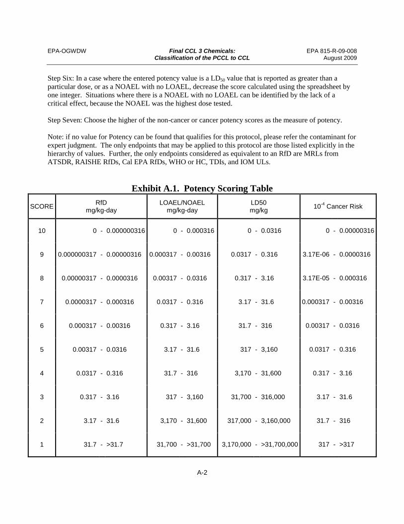
EPA-OGWDW Final CCL 3 Chemicals: EPA 815-R-09-008 Classification of the PCCL to CCL August 2009
Step Six: In a case where the entered potency value is a LD50 value that is reported as greater than a particular dose, or as a NOAEL with no LOAEL, decrease the score calculated using the spreadsheet by one integer. Situations where there is a NOAEL with no LOAEL can be identified by the lack of a critical effect, because the NOAEL was the highest dose tested.
Step Seven: Choose the higher of the non-cancer or cancer potency scores as the measure of potency.
Note: if no value for Potency can be found that qualifies for this protocol, please refer the contaminant for expert judgment. The only endpoints that may be applied to this protocol are those listed explicitly in the hierarchy of values. Further, the only endpoints considered as equivalent to an RfD are MRLs from ATSDR, RAISHE RfDs, Cal EPA RfDs, WHO or HC, TDIs, and IOM ULs.
Exhibit A.1. Potency Scoring Table
SCORE RfD mg/kg-day
LOAEL/NOAEL mg/kg-day
LD50 mg/kg 10-4 Cancer Risk
10
9
8
7
6
5
4
3
2
1
0 - 0.000000316
0.000000317 - 0.00000316
0.00000317 - 0.0000316
0.0000317 - 0.000316
0.000317 - 0.00316
0.00317 - 0.0316
0.0317 - 0.316
0.317 - 3.16
3.17 - 31.6
31.7 - >31.7
0 - 0.000316
0.000317 - 0.00316
0.00317 - 0.0316
0.0317 - 0.316
0.317 - 3.16
3.17 - 31.6
31.7 - 316
317 - 3,160
3,170 - 31,600
31,700 - >31,700
0 - 0.0316
0.0317 - 0.316
0.317 - 3.16
3.17 - 31.6
31.7 - 316
317 - 3,160
3,170 - 31,600
31,700 - 316,000
317,000 - 3,160,000
3,170,000 - >31,700,000
0 - 0.00000316
3.17E-06 - 0.0000316
3.17E-05 - 0.000316
0.000317 - 0.00316
0.00317 - 0.0316
0.0317 - 0.316
0.317 - 3.16
3.17 - 31.6
31.7 - 316
317 - >317
A-2

EPA-OGWDW Final CCL 3 Chemicals: EPA 815-R-09-008 Classification of the PCCL to CCL August 2009
A.2 Severity Scoring Protocol
The score for Severity is based upon the critical effect associated with the data element (RfD, LOAEL, etc.) used to score Potency. Potency must be scored prior to Severity.
Protocol for Severity Scoring Step One: Identify the critical effect for the contaminant, based on the data used to score the
attribute of potency, and enter it into the severity scoring worksheet (shown in Exhibit A.2). If the contaminant has more than one critical effect all of the listed effects should be included. NOTE: If the critical effect is death and the LD50 data element was used to score potency, go to Step Four. If the effects are for a LOAEL from RTECS go to Step Five.
Step Two: Locate the critical effect within the Compendium of Critical Effects Table (see Exhibit A.3) and enter the severity score associated with that critical effect in the severity scoring worksheet. If a contaminant has more than one critical effect, choose the highest of the scores. NOTE: If the critical effect is not listed in the Table, go to Step Three.
Step Three: If the critical effect is not listed in the Table, the scorer should flag that critical effect as ‘not listed.’ (Health effects experts should be consulted to score these effects.) Once the effect is scored it should be added to the compendium for future use and consistent scoring.
Step Four: If a critical effect is not available, or is “death,” use one of the following options for scoring: 1) Search sources identified as supplemental sources for CCL for additional health
effects data that could be used to score potency and severity for the contaminant. If data are found that provide a data element from the potency protocol other than LD50 to score the contaminant, then that element can be used for scoring. Sources that may be most helpful in this search include: Hazardous Substances Data Bank (HSDB), International Program on Chemical Safety (INCHEM), and the National Toxicology Program (NTP). The element that is found may be used to rescore the contaminant for potency, and subsequently severity, using the score associated with the critical effect endpoint.
2) Search for an alternative critical effect associated with the LD50 determination. Locate the LD50 study and search for information regarding the types of effects occurring prior to animal death. If a critical effect other than death is given in the study, it may be used to score the severity of the contaminant. (The potency score is still given by the value of the LD50.)
3) If no additional information can be found, recommend that the contaminant be returned to the Universe.
Step Five If the Potency score is a LOAEL from RTECS, the effects listed represent all effects and
A-3

EPA-OGWDW Final CCL 3 Chemicals: EPA 815-R-09-008 Classification of the PCCL to CCL August 2009
not just the critical effect (s). There are three available options for improving the scoring in this situation.
1. If the RTECS data source is included in the supplemental data, review the supplemental information to identify the critical effect. If the supplemental source includes a NOAEL for the critical effect, replace the LOAEL with the NOAEL and rescore potency if necessary.
2. In cases where the data source for the LOAEL is not in the supplemental data search the supplemental data for an alternative data source. If the data identified provides a NOAEL or LOAEL that is the same or lower than that in RTECS or is from a study of higher quality than the RTECS study , use that NOAEL or LOAEL and its critical effect to score both potency and severity.
3. If it is not possible to find better information in the supplemental data sources score the most serious of the effects listed in RTECS.
Exhibit A.2. Severity Scoring Table Key Study used to score Potency Critical Effect(s) for Severity Severity Score
1 2 3 4 5 6 7 8 9
10 11 12 13 14 15 16 17 18 19 20 21 22 23 24 25
A-4

EPA-OGWDW Final CCL 3 Chemicals: EPA 815-R-09-008 Classification of the PCCL to CCL August 2009
Exhibit A.3. Compendium of Critical Effects Table (from Health Advisories & IRIS) For Scoring Severity
Severity Score
Score Definition Compendium of Critical Effects
1 NO ADVERSE EFFECT No observed effect(s). No observed adverse effect(s). Absence of effects. No critical effect(s) identified. No effect(s) related to treatment. Absence of biologically significant adverse effect(s). Absence of gross light microscopic histopathological
change(s). Excedance of the Taste Threshold
2 COSMETIC EFFECT (Interpretation: Consider those effects that alter the appearance of the body without affecting structure or functions)
Dental fluorosis. Abnormal appearance. Facial flushing. Flushing. Argyria. Dermal sensitization. Skin pigmentation. Hyperpigmentation. Alopecia. Keratosis.
3 REVERSIBLE EFFECTS; DIFFERENCES IN ORGAN WEIGHTS OR SIZE, BODY WEIGHTS OR CHANGES IN BIOCHEMICAL PARAMETERS WITH MINIMAL CLINICAL SIGNIFICANCE. (Interpretation: Transient, adaptive effects)
Growth and Weight Effects Decreased body weight and or body-weight gain. Increased absolute organ weights. Increased liver weight. Increased kidney weight. Increased relative organ weight. Decreased relative organ weight. Lower ovarian weight. Decreased maternal weight gain. Increased absolute and relative (to body and/or brain)
liver weight. Increased kidney body weight ratio. Increase in spleen weight. Increase in thyroid/body weight ratio. Changes in thymus weight. Decreased body weight. Decreased growth.
Gastrointestinal Disturbances Decreased stool quantity. Osmotic diarrhea. Diarrhea. Nausea. Vomiting. GI irritation. GI disturbances.
A-5

EPA-OGWDW Final CCL 3 Chemicals: EPA 815-R-09-008 Classification of the PCCL to CCL August 2009
Exhibit A.3. Compendium of Critical Effects Table (from Health Advisories & IRIS) For Scoring Severity
Severity Score
Score Definition Compendium of Critical Effects
3 (cont.) Irritation/Irritability Chronic irritation. Maternal hyperirritability. Chronic irritation without histopathology changes.
Biochemical Changes Decreased glucose. Increased blood sugar. Increased enzymes. Increased triglycerides. Increase serum concentration of compound. Clinical serum effects. Alterations in clinical chemistry. Increased serum alkaline phosphatase. Significant elevation of serum calcium levels. Enzyme inhibition, induction, or change in blood
tissue levels Decreased ESOD activity. Decrease in erythrocyte superoxide dismutase
(ESOD) concentration. Minor alteration in clinical chemistry, e.g., decrease
in erythrocyte superoxide dismutase (ESOD). Hematological effects
Hematological effects. Abnormal pigments in blood. Decreased lymphocyte count. Decreased blood counts. Decreased white blood cells. Methemoglobinemia. Increased carboxyhemoglobin. Hemosiderosis. Anemia. Normocytic anemia. Iron deposits and elevated Heinz bodies in liver. Decreased hemoglobin and possible erythrocyte
destruction. Decreased RBC, packed cell volume, and
hemoglobin. Hematologic, hepatic, and renal toxicity as evidenced
by a statistically significant decrease in hemoglobin, hematocrit, and RBC levels.
RBC and liver effects as evidenced by increase Heinz bodies in RBC.
Sporadic decrease in hemoglobin and RBC. Decreased RBC and hematocrit.
A-6

EPA-OGWDW Final CCL 3 Chemicals: EPA 815-R-09-008 Classification of the PCCL to CCL August 2009
Exhibit A.3. Compendium of Critical Effects Table (from Health Advisories & IRIS) For Scoring Severity
Severity Score Definition Compendium of Critical Effects Score
3 (cont.) Cholinesterase Effects Reversible PChE (plasma) or RBC-ChE inhibition
without cholinergic symptoms or signs RBC ChE depression without cholinergic symptoms
or sweating. Plasma cholinesterase (ChE) inhibition without
cholinergic symptoms or sweating. Hormone Changes
Decrease in T3, T4. Dose-related decrease in T4, T3, and increase TSH. Elevated thyroid stimulating hormone (TSH)
concentration. ACTH decrease.
Cellular Vacuolization Mild to moderate vacuolization Tubular epithelial vacuolization. Brain cell vacuolization.
Additional Effects Changes in teeth and supporting structures. Sensory organ effects. Centrilobular eosinophilic liver changes. Possible vascular complication. Inhibition of the concentration of beneficial bacteria
in the gastrointestinal microflora 4 CELLULAR/PHYSIOLOGICAL Hematological Effects
CHANGES THAT COULD Jaundice. LEAD TO DISORDERS (risk Anemia factors or precursor effects). Hemolytic anemia. (Interpretation: Considers Erythrocyte destruction. cellular/physiological changes in the Hemolysis. body that are used as indicators of disease susceptibility)
Immunological Effects Decreased delayed hypersensitivity response. Decrease in cellular immune response. Decrease in humoral immune response.
Liver Effects Fatty cyst - liver and elevated liver enzymes (i.e.,
SGPT, LDH). Liver cell enlargement or alteration. Liver cell polymorphism. Proteinuria. Renal cytomegaly.
Cholinergic Effects Cholinesterase inhibition with symptoms. Cholinergic signs or symptoms.
Other Effects
A-7

EPA-OGWDW Final CCL 3 Chemicals: EPA 815-R-09-008 Classification of the PCCL to CCL August 2009
Exhibit A.3. Compendium of Critical Effects Table (from Health Advisories & IRIS) For Scoring Severity
Severity Score
Score Definition Compendium of Critical Effects
Hypothermia Mild CNS Effects
5 SIGNIFICANT FUNCTIONAL CHANGES THAT ARE REVERSIBLE OR PERMANENT CHANGES OF MINIMAL TOXICOLOGICAL SIGNIFICNACE. (Interpretation: Consider those disorders in which the removal of chemical exposure will restore health back to prior condition)
Increased cholinergic effects ChE inhibition with sweating, diarrhea, hypotention,
and/or fishy body odor.. RBC and/or plasma acetylcholinesterase (AChE)
inhibition with cholinergic symptoms or sweating. Brain acetylcholineesterase inhibition with or without
signs or symptoms Hematological Effects
GI bleeding. Coagulation defects. Extramedulary hematopoesis Tendency to hemorrhage.
Structural Effects Rachitic bone.
Renal Effects Renal cytomegaly. Renal effects/toxicity (increased uric acid levels;
increased urinary coproporphyrins). Inflammatory foci – kidneys.
Hepatic Effects Liver function tests impaired. Fatty-cyst in liver hemosiderosis.
Multiple Organ Effects Effects on the lungs, liver, kidney, thyroid and
thyroid hormones. Ocular Effects
Corneal damage. Neurological Effects
Mild neurological signs. Alteration of classic conditioning. Brain ChE inhibition. Myelin degeneration. CNS depression. Brain/ other coverings- recordings from specific
areas of CNS. Tremors. Dyspnea. Changes in motor activity. Hypoactivity. Ataxia.
A-8

EPA-OGWDW Final CCL 3 Chemicals: EPA 815-R-09-008 Classification of the PCCL to CCL August 2009
Exhibit A.3. Compendium of Critical Effects Table (from Health Advisories & IRIS) For Scoring Severity
Severity Score
Score Definition Compendium of Critical Effects
5 (cont.) Other Effects Chronic pneumonitis. Clinical selenosis. Nonneoplastic lesions - splenic capsule. Intestinal lesions. Splenomegaly
6 SIGNIFICANT, IRREVERSIBLE, NONLETHAL CONDITIONS OR DISORDERS. (Interpretation: Consider those disorders that persist for over a long period of time but do not lead to death)
Multiple Organ Effects Histopathological effects in liver, kidney, and thyroid. Minimal to moderate congestion of liver, kidney, and
lungs. Liver and kidney pathology. Kidney and spleen pathology.
Hepatic Effects Hepatic lesions/necrosis. Hepatocyte degeneration. Hepatotoxicity. Liver cell polymorphism. Liver effects/toxicity. Liver lesions.
Renal Effects Atrophy and degeneration of the renal tubules –
nephropathy (unspecified). Kidney toxicity. Mineralization of the kidneys. Renal dysfunction. Renal effects/toxicity (increased uric acid levels;
increased urinary coproporphyrins). Functional and histopathological effects in kidney. Kidney damage (unspecified). Kidney lesions (unspecified). Impaired renal clearance/function. Tubular epithelial vacuolation.
Sensory and Neurological Effects Significant decrease in brain and brain to body
weight ratio. Degenerative changes for brain/ other coverings. Peripheral neuropathy- neuropathy (unspecified). Neurotoxicity. Nerve damage (unspecified). Optic nerve degeneration/ damage. Sensory neuropathy. Minimal lens opacity and cataracts. Nasal olfactory lesions.
A-9

EPA-OGWDW Final CCL 3 Chemicals: EPA 815-R-09-008 Classification of the PCCL to CCL August 2009
Exhibit A.3. Compendium of Critical Effects Table (from Health Advisories & IRIS) For Scoring Severity
Severity Score
Score Definition Compendium of Critical Effects
6 (cont.) Hyperplasia Thyroid hyperplasia. Urothelial hyperplasia. Hyperplasia. Squamous and basal hyperplasia of the
forestomach. Epithelial hyperplasia – forestomach.
Cardiac Effects Cardiac toxicity. Cardiomyopathy, including infarction. Vascular complications. Right atrial dilation. Convulsions. Mild histological lesions.
Other Effects Gastrointestinal necrotic changes. Chronic irritation with histopathology findings. Forestomach lesions (unspecified). Organ atrophy. Thyroid effects (unspecified). Thyroid mineralization. Spleen toxicity (unspecified). Bladder toxicity (unspecified). Bone marrow toxicity (unspecified). Hormonal response to extrogenic substances in post menopausal women.
7 DEVELOPMENTAL OR REPRODUCTIVE EFFECTS LEADING TO MAJOR DYSFUNCTION. (Interpretation: Considers those chemicals that cause permanent developmental effects or that impact the ability of a population to reproduce)
Reproductive Organ Effects Testicular atrophy/damage. Testicular and uterine effects. Atrophied seminiferous epithelium. Histopathological changes in testes. Hypospadia. Lesions observed in reproductive organs. Decreased testes weight and testes to body weight
ratio, atrophied seminiferous epithelium; and decreased tubular size in testes.
Endometriosis. Decreased tubular size in testes. Decreased ovarian weight and function. Altered cellular foci.
Maternal Toxicity Maternal toxicity. Decreased maternal weight gain.
A-10

EPA-OGWDW Final CCL 3 Chemicals: EPA 815-R-09-008 Classification of the PCCL to CCL August 2009
Exhibit A.3. Compendium of Critical Effects Table (from Health Advisories & IRIS) For Scoring Severity
Severity Score
Score Definition Compendium of Critical Effects
7 (cont.) Fertility effects
Spermatogenic arrest. Reduced numbers of corpora allata. Reduced or deformed sperms. Adverse reproductive effects. Reduction in fertility. Decreased fertility index. Decrease in size of litter.
Growth inhibition Reduced offspring weight gain, total litter weight, or
litter size. Decreased pup weight Decreased lactation indices. Increased runt incidence. Decreased crown-rump length
Decreased offspring viability Excessive loss of litters Increase in number of stillbirths. Maternal and fetal toxicity. Increased intrauterine death. Decreased pup survival or viability. Increased abortion rate. Increase in number of stillbirths. Increased dead pups at birth. Decreased pup viability index. Parturition mortality. Fetal resorptions.
Developmental effects Fetal toxicity/malformations. Developmental toxicity (skeletal or visceral
abnormalities). Delayed ossification. Neurodevelopmental effects. Brain cell vacuolization in neonates. Myelin degeneration. Skeletal or visceral abnormalities (Extra ribs and
other measures of sexual maturation). Increased retinal folds in weanlings. Mixed sexual differentiation (i.e., effeminization or
emasculanization). Imbalance in sex ratio.
8 TUMORS OR DISORDERS LIKELY LEADING TO DEATH (Interpretation: Considers chemical exposures that result in a fatal disorder and all types of tumors).
Cancer. Suspected carcinogenicity (including short latency
periods and rare tumors). Any type of cancer.
A-11
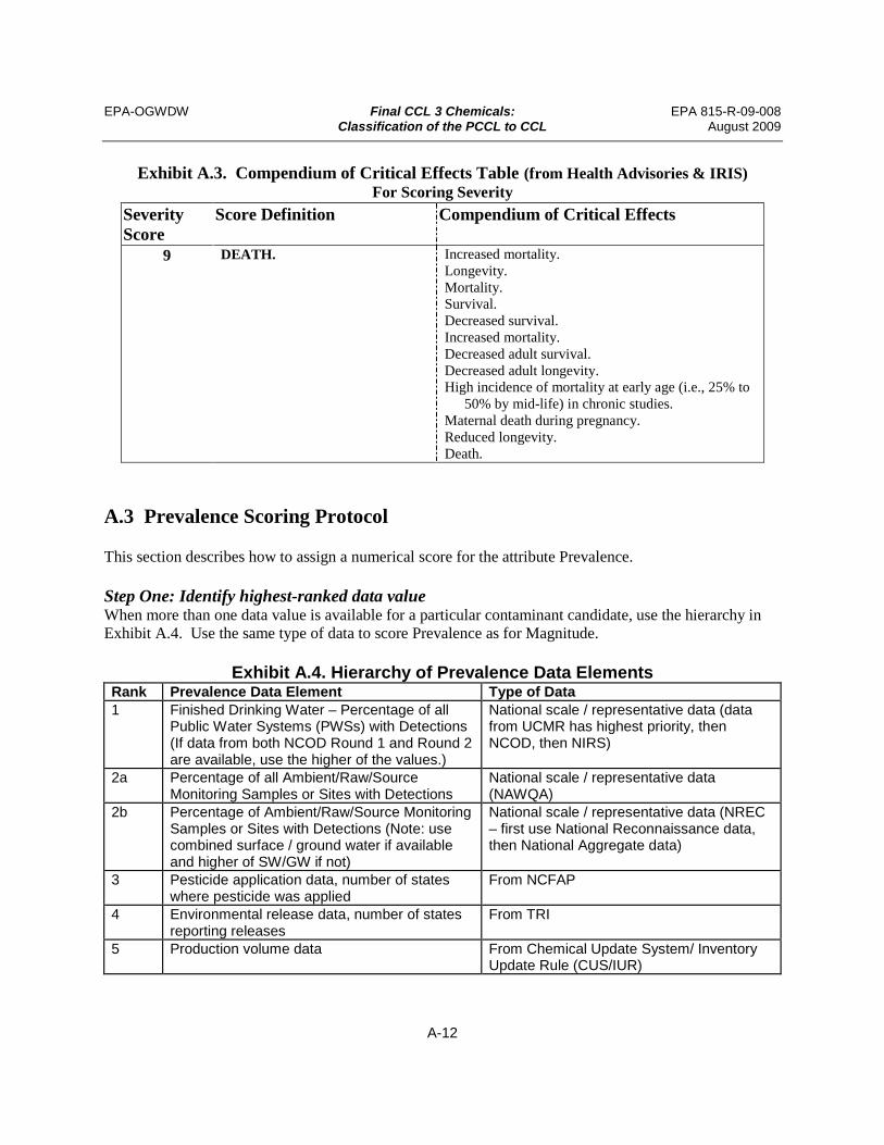
EPA-OGWDW Final CCL 3 Chemicals: EPA 815-R-09-008 Classification of the PCCL to CCL August 2009
Exhibit A.3. Compendium of Critical Effects Table (from Health Advisories & IRIS) For Scoring Severity
Severity Score
Score Definition Compendium of Critical Effects
9 DEATH. Increased mortality. Longevity. Mortality. Survival. Decreased survival. Increased mortality. Decreased adult survival. Decreased adult longevity. High incidence of mortality at early age (i.e., 25% to
50% by mid-life) in chronic studies. Maternal death during pregnancy. Reduced longevity. Death.
A.3 Prevalence Scoring Protocol
This section describes how to assign a numerical score for the attribute Prevalence.
Step One: Identify highest-ranked data value When more than one data value is available for a particular contaminant candidate, use the hierarchy in Exhibit A.4. Use the same type of data to score Prevalence as for Magnitude.
Exhibit A.4. Hierarchy of Prevalence Data Elements Rank Prevalence Data Element Type of Data 1 Finished Drinking Water – Percentage of all
Public Water Systems (PWSs) with Detections (If data from both NCOD Round 1 and Round 2 are available, use the higher of the values.)
National scale / representative data (data from UCMR has highest priority, then NCOD, then NIRS)
2a Percentage of all Ambient/Raw/Source Monitoring Samples or Sites with Detections
National scale / representative data (NAWQA)
2b Percentage of Ambient/Raw/Source Monitoring Samples or Sites with Detections (Note: use combined surface / ground water if available and higher of SW/GW if not)
National scale / representative data (NREC – first use National Reconnaissance data, then National Aggregate data)
3 Pesticide application data, number of states where pesticide was applied
From NCFAP
4 Environmental release data, number of states reporting releases
From TRI
5 Production volume data From Chemical Update System/ Inventory Update Rule (CUS/IUR)
A-12

EPA-OGWDW Final CCL 3 Chemicals: EPA 815-R-09-008 Classification of the PCCL to CCL August 2009
Step Two: Use scoring table to find attribute score for value identified in Step One. For each element there is a corresponding column in the Prevalence Scoring table (see Exhibit A.5), which contains a range of data values assigned to a numeric prevalence score between 1 and 10. Once a data value has been found for a particular element, look up the value in Exhibit A.5 to determine the prevalence score. For CUS/IUR data, use the most recent year reported. For pesticides, if the compound is a degradate and does not have its own data, use the parent to score.
Exhibit A.5. Prevalence Scoring Scales
Hierarchy
Prevalence Score
1 2 3 4 5
% Finished Water PWSs
with detections of contaminant
All PWSs
% Ambient water sites
with detections of contaminant
All sites/samples
# States Reporting Pesticide in Use # of States
Reporting TRI total releases
CUS/IUR (production data)
Number of pounds (by category)
produced
1 <=0.10 <=0.10 - 1 <500K 2 0.11-0.16 0.11-0.16 - 2 -
3 0.17-0.25 0.17-0.25
Default for any pesticide in non-
environmental use 3 >500K-1M 4 0.26-0.44 0.26-0.44 - 4 -
5 0.45-0.61 0.45-0.61
Default for any pesticide in
environmental use without data 5 >1M-10M
6 0.62-1.00 0.62-1.00 <6 6 >10M-50M 7 1.01-1.30 1.01-1.30 6-10 7-10 >50M-100M 8 1.31-2.50 1.31-2.50 11-15 11-15 >100M-500M 9 2.51-10.00 2.51-10.00 16-25 16-25 >500M-1B 10 >10.00 >10.00 >25 >25 >1B
Note: Use data in the highest category to score. For CUS/IUR data, use the most recent year reported. Not Reported means there has been no change in production volume since the last report. For pesticides, if the compound is a degradate and does not have its own data, use the parent to score.
A-13
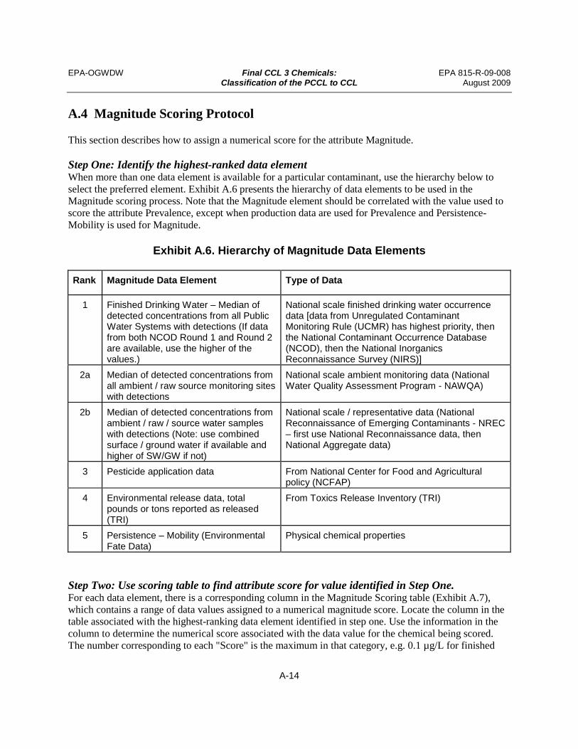
EPA-OGWDW Final CCL 3 Chemicals: EPA 815-R-09-008 Classification of the PCCL to CCL August 2009
A.4 Magnitude Scoring Protocol
This section describes how to assign a numerical score for the attribute Magnitude.
Step One: Identify the highest-ranked data element When more than one data element is available for a particular contaminant, use the hierarchy below to select the preferred element. Exhibit A.6 presents the hierarchy of data elements to be used in the Magnitude scoring process. Note that the Magnitude element should be correlated with the value used to score the attribute Prevalence, except when production data are used for Prevalence and Persistence-Mobility is used for Magnitude.
Exhibit A.6. Hierarchy of Magnitude Data Elements
Rank Magnitude Data Element Type of Data
1 Finished Drinking Water – Median of detected concentrations from all Public Water Systems with detections (If data from both NCOD Round 1 and Round 2 are available, use the higher of the values.)
National scale finished drinking water occurrence data [data from Unregulated Contaminant Monitoring Rule (UCMR) has highest priority, then the National Contaminant Occurrence Database (NCOD), then the National Inorganics Reconnaissance Survey (NIRS)]
2a Median of detected concentrations from all ambient / raw source monitoring sites with detections
National scale ambient monitoring data (National Water Quality Assessment Program - NAWQA)
2b Median of detected concentrations from ambient / raw / source water samples with detections (Note: use combined surface / ground water if available and higher of SW/GW if not)
National scale / representative data (National Reconnaissance of Emerging Contaminants - NREC – first use National Reconnaissance data, then National Aggregate data)
3 Pesticide application data From National Center for Food and Agricultural policy (NCFAP)
4 Environmental release data, total pounds or tons reported as released (TRI)
From Toxics Release Inventory (TRI)
5 Persistence – Mobility (Environmental Fate Data)
Physical chemical properties
Step Two: Use scoring table to find attribute score for value identified in Step One. For each data element, there is a corresponding column in the Magnitude Scoring table (Exhibit A.7), which contains a range of data values assigned to a numerical magnitude score. Locate the column in the table associated with the highest-ranking data element identified in step one. Use the information in the column to determine the numerical score associated with the data value for the chemical being scored. The number corresponding to each "Score" is the maximum in that category, e.g. 0.1 µg/L for finished
A-14

EPA-OGWDW Final CCL 3 Chemicals: EPA 815-R-09-008 Classification of the PCCL to CCL August 2009
water scores 4, not 5. In cases where there are no data for Scoring Magnitude in Exhibit A.7 (e.g. Prevalence is scored using Production Volume data), use the Persistence-Mobility Scoring approach to develop a Magnitude Score.
Persistence-Mobility Scoring
The approach for scoring persistence and mobility includes assigning two values, one for persistence and one for mobility, on a numeric scale of 1 through 3, representing low, medium, and high for each property as it favors the presence of the contaminant in water. Using a hierarchy of physical property data elements, each contaminant is scored for both persistence and mobility. The average of these two values is multiplied by 10/3 to obtain the persistence-mobility score. Exhibit A.8 displays the hierarchy of available properties for each data element representing either persistence or mobility.
Protocol for Persistence-Mobility Scoring
Step One: Identify and score highest-ranked data value for Persistence When more than one data element value is available for a particular contaminant candidate, use the hierarchy below to select the preferred element. Exhibit A.6 describes the hierarchy of data elements to be used in the Persistence scoring process. When several values for a physical property are available, the highest scoring value should be used, unless that value is not representative of environmental conditions in drinking water.
Step Two: Identify and score highest-ranked data value for Mobility The hierarchy of physical properties for scoring mobility is given in Exhibit A.6. Select the highest priority data element available for scoring. When several values for a particular physical property are available, the highest scoring value should be used for scoring, unless that value is not representative of environmental conditions in drinking water.
Step Three: Multiply the average of the persistence and mobility values by 10/3 for the magnitude score.
A-15

EPA-OGWDW Final CCL 3 Chemicals: EPA 815-R-09-008 Classification of the PCCL to CCL August 2009
Exhibit A.7. Magnitude Scoring Scales
Hierarchy
Magnitude Scale
1 2 3 4 5 Finished Water
Occurrence Scale
Ambient Water Occurrence
Scale
Pesticide Use Scale
TRI Total Releases Scale
Persistence/ Mobility
Data Used to Score
Median of detections - all
PWSs
Median of detections - all sites/samples
Number of pounds applied
Total number of pounds released
Units µg/L µg/L lbs lbs Used when Production
data are used to score for prevalence.
See Persistence/
Mobility protocol
(Exhibit A.8)
Score 1 <0.003 <0.003 <10,000 <300
2 0.003 - 0.01 0.003 - 0.01 - 301-1,000 3 >0.01 - 0.03 >0.01 - 0.03 10,000-30,000 1,001-3,000 4 >0.03 - 0.1 >0.03 - 0.1 30,001-100,000 3,001-10,000 5 >0.1 - 0.3 >0.1 - 0.3 100,001-300,000 10,001-30,000 6 >0.3 - 1 >0.3 – 1 300,001-1M 30,001-100,000 7 >1 - 3 >1 – 3 1M - 3M 100,001-300,000 8 >3 - 10 >3 – 10 3M - 10M 300,001-1M 9 >10 - 30 >10 – 30 10M - 30M 1M - 3M
10 >30 >30 >30M >3M
Notes: Use data in the highest category to score. The number corresponding to each "Score" is the maximum in that category, e.g. 0.1 µg/L scores 4, not 5. For pesticides, use the parent to score if the compound is a degradate and does not have its own data.
Exhibit A.8. Magnitude Scales for Environmental Fate Data Magnitude Hierarchy 5 Mobility Scale Value
Units 1 (Low) 2 (Medium) 3 (High) Organic Carbon Partitioning Coefficient (Koc) mL/g >1,000 100-1,000 <100 Log Octanol/Water Partitioning Coefficient (log Kow) dimensionless >4 1-4 <1 Soil/Water Distribution Coefficient (Kd) mL/g >10 1-10 <1 Henry's Law Coefficient (KH) atm-m3/mol >10-3 10-7-10-3 <10-7
Henry's Law Coefficient (KH) dimensionless >0.042
0.0424.2x10-6 <4.2x10⁻⁶
A-16
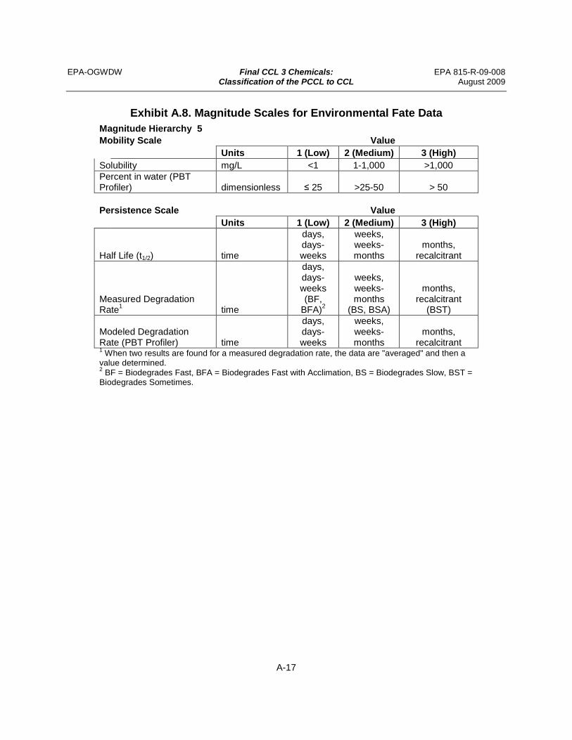
EPA-OGWDW Final CCL 3 Chemicals: EPA 815-R-09-008 Classification of the PCCL to CCL August 2009
Exhibit A.8. Magnitude Scales for Environmental Fate Data Magnitude Hierarchy 5 Mobility Scale Value
Solubility Percent in water (PBT Profiler)
Units mg/L
dimensionless
1 (Low) <1
≤ 25
2 (Medium) 1-1,000
>25-50
3 (High) >1,000
> 50
Persistence Scale Value Units 1 (Low) 2 (Medium) 3 (High)
Half Life (t1/2) time
days, days-weeks
weeks, weeks-months
months, recalcitrant
Measured Degradation Rate1 time
days, days-weeks (BF,
BFA)2
weeks, weeks-months
(BS, BSA)
months, recalcitrant
(BST)
Modeled Degradation Rate (PBT Profiler) time
days, days-weeks
weeks, weeks-months
months, recalcitrant
1 When two results are found for a measured degradation rate, the data are "averaged" and then a value determined. 2 BF = Biodegrades Fast, BFA = Biodegrades Fast with Acclimation, BS = Biodegrades Slow, BST = Biodegrades Sometimes.
A-17

EPA-OGWDW Final CCL 3 Chemicals: EPA 815-R-08-008 Classification of the PCCL to CCL August 2009
Contaminant 3
Appendix B. Example Blinded Information Sheets from the TDS Exercises
Contaminant Name:
It is a volatile organic chemical. It is used as a wetting and dispersing agent in textile processing, dye-baths, stain and printing compositions; used in cleaning and detergent preparations, adhesives, cosmetics, deodorants, fumigants, emulsions and polishing compositions. Used in lacquers, paints, varnishes, paint and varnish removers. Degreasing agent. It is on the TSCA list. The reportable released quanitity of this substance under CERCLA is 1 lb. It is also subject to RCRA waste management requirements, and is listed as a hazardous air pollutant by EPA. Several states have drinking water guidelines for this chemical (CA, FL, MA, ME, NC). Its one-day Health Advisory Level (HAL) is 4,000 µg/L, its 10-day HAL is 400 µg/L, and its 10^-4 cancer risk HAL is 300 µg/L. This is an HPV chemical. It is also on the
Background:
CCL. (HSDB, 2005; EPAHA, 2004)
HEALTH EFFECTS DATA Data Element Value Units Source Notes Reference Dose N/A
Carcinogen classification (EPA) B2 (probable human carcinogen) IRIS 9/1/1990 Slope Factor 0.011 1/(mg/kg-d) IRIS 9/1/1990
Carcinogen Classification (IARC) 2B (possible) IARC
Non EPA Derived Dose1 0.1 mg/kg-d ATSDR MRL Chronic oral Critical Effect Hepatic effects UF=100 File/Issue Date 10/1/2004
Lowest Oral Chronic LOAEL1 N/A
Lowest Oral LD501 N/A
Is contaminant on list of carcinogens? Y Y/N Cal EPA Chemicals Known to the State to Cause Cancer or Reproductive Toxicity
1/1/1988
Is the contaminant on a list of reproductive toxins? N Y/N
Cal EPA Chemicals Known to the State to Cause Cancer or Reproductive Toxicity
Risk assessment ongoing? Y Y/N
Health Reference Level (HRL)2 700 µg/L Based on MRL Health Reference Level (HRL)2 cancer 3.18 µg/L Health Reference Level (HRL) cancer 300 µg/L 10-4 cancer risk Health Advisory (EPAHA, 1987) Notes 1 Non-EPA toxicology data will be sought if no EPA Reference Dose or carcinogen information available; may require multiple entries; chronic studies will be prioritized over short term studies. 2 Health Reference Level calculated by conversion of RfD or other dose to units of µg/L, assuming 2 liters per day of water consumed by a 70 Kg adult, and a default Relative Source Contribution of 20%. For carcinogens, the concentration at the 10-6 cancer risk level will be converted to units of µg/L and will also be listed.
B-1
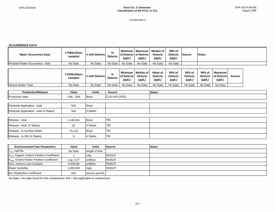
EPA-OGWDW Final CCL 3 Chemicals: EPA 815-R-08-008 Classification of the PCCL to CCL August 2009
Contaminant 3
OCCURRENCE DATA
Water Occurrence Data # PWSs/Sites sampled # with Detects %
Detects
Minimum of Detects
(µg/L)
Maximum of Detects
(µg/L)
Median of Detects (µg/L)
99% of Detects (µg/L)
Source Notes
Finished Water Occurrence - total No Data No Data No Data No Data No Data No Data No Data
# PWSs/Sites sampled # with Detects %
Detects
Minimum of Detects
(µg/L)
Median of Detects (µg/L)
Mean of Detects (µg/L)
90% of Detects (µg/L)
95% of Detects (µg/L)
99% of Detects (µg/L)
Maximum of Detects
(µg/L) Source
Source Water-Total No Data No Data No Data No Data No Data No Data No Data No Data No Data No Data
Production/Release Value Units Source Notes Production data >1M - 10M lbs/yr CUS-IUR (2002)
Pesticide Application - total N/A lbs/yr
Pesticide Application - total (# States) N/A # States
Release - total 1,146,641 lbs/yr TRI
Release - total (# States) 22 # States TRI
Release - to Surface Water 75,119 lbs/yr TRI
Release - to SW (# States) 9 # States TRI
Environmental Fate Parameters Value Units Source Notes T1/2, Half life No Data length of time KOC, Organic Carbon Partition Coefficient 1 L/kg RAISCF KOW, Octanol Water Partition Coefficient Log -0.27 unitless RAISCF HLC, Henry's Law Constant 0.000196 unitless RAISCF Water Solubility 1,000,000 mg/L RAISCF
Kd, Distribution Coefficient N/A source specific
No Data = No data found for this contaminant; N/A = Not applicable to contaminant
B-2

EPA-OGWDW Final CCL 3 Chemicals: EPA 815-R-08-008 Classification of the PCCL to CCL August 2009
Contaminant 4
Contaminant Name:
Background: This is a volatile organic chemical. It is used as a food additive, organic intermediate, solvent, and in cosmetic formulations. It is also used as a solvent or solubilizer in the paint and printing ink sector, as components in textile auxiliaries and pesticides, for hormone extraction, and in the surfactant field as foam boosters or antifrothing agents. Per the FDA, this food additive is permitted for direct addition to food for human consumption as a synthetic flavoring substance and adjuvant. (HSDB, 2005)
HEALTH EFFECTS DATA Data Element Value Units Source Notes Reference Dose N/A
Carcinogen classification (EPA) N/A Slope Factor N/A
Carcinogen Classification (IARC) N/A
Non EPA Derived Dose1 N/A
Lowest Oral Chronic LOAEL1 N/A
Lowest Oral LD501 500 mg/kg RTECS Critical effect: Ataxia, irritability, dyspnea, acute pulmonary edema
Is contaminant on list of carcinogens? N Y/N Cal EPA Chemicals Known to the State to Cause Cancer or Reproductive Toxicity
Is the contaminant on a list of reproductive toxins? N Y/N
Cal EPA Chemicals Known to the State to Cause Cancer or Reproductive Toxicity
Risk assessment ongoing? N Y/N
Health Reference Level (HRL)2 N/A µg/L Health Reference Level (HRL)2 cancer N/A µg/L Notes 1 Non-EPA toxicology data will be sought if no EPA Reference Dose or carcinogen information available; may require multiple entries; chronic studies will be prioritized over short term studies. 2 Health Reference Level calculated by conversion of RfD or other dose to units of µg/L, assuming 2 liters per day of water consumed by a 70 Kg adult, and a default Relative Source
Contribution of 20%. For carcinogens, the concentration at the 10-6 cancer risk level will be converted to units of µg/L and will also be listed.
B-3

EPA-OGWDW Final CCL 3 Chemicals: EPA 815-R-08-008 Classification of the PCCL to CCL August 2009
Contaminant 4
OCCURRENCE DATA
Water Occurrence Data # PWSs/Sites sampled # with Detects %
Detects
Minimum of Detects
(µg/L)
Maximum of Detects
(µg/L)
Median of Detects (µg/L)
99% of Detects (µg/L)
Source Notes
Finished Water Occurrence - total No Data No Data No Data No Data No Data No Data No Data
# PWSs/Sites sampled # with Detects %
Detects
Minimum of Detects
(µg/L)
Median of Detects (µg/L)
Mean of Detects (µg/L)
90% of Detects (µg/L)
95% of Detects (µg/L)
99% of Detects (µg/L)
Maximum of Detects
(µg/L) Source
Source Water-Total No Data No Data No Data No Data No Data No Data No Data No Data No Data No Data
Production/Release Value Units Source Notes Production data >500K - 1M lbs/yr CUS-IUR (2002)
Pesticide Application - total N/A lbs/yr
Pesticide Application - total (# States) N/A # States
Release - total No Data lbs/yr
Release - total (# States) No Data # States
Release - to Surface Water No Data lbs/yr
Release - to SW (# States) No Data # States
Environmental Fate Parameters Value Units Source Notes T1/2, Half life No Data length of time KOC, Organic Carbon Partition Coefficient 15 L/kg HSDB KOW, Octanol Water Partition Coefficient Log 2.62 unitless HSDB HLC, Henry's Law Constant 1.88E-05 atm-cu m/mol HSDB Water Solubility 1000 mg/L HSDB
Kd, Distribution Coefficient N/A source specific
No Data = No data found for this contaminant; N/A = Not applicable to contaminant
B-4

EPA-OGWDW Final CCL 3 Chemicals: EPA 815-R-08-008 Classification of the PCCL to CCL August 2009
Contaminant 5
Contaminant Name:
Background: This is a volatile organic chemical registered for use in the U.S. Nematicide. Seventh most commonly used pesticide in U.S. agricultural crop production. Used in organic synthesis and in manufacture of pesticides. Pre-plant soil fumigant. It is listed on FIFRA and TSCA. The reportable release quantity under CERCLA is 100 lbs. It is subject to RCRA waste management requirements. It is listed as a hazardous air pollutant and as a hazardous substance by the Federal Water Pollution Control Act and the Clean Water Act. It has a state drinking water standard in CA. It has a state drinking water guideline in several states (FL, MA, ME, MN, WI). It has a DWEL of 1,000 µg/L, and its one-day and ten-day Health Advisory Levels (HALs) are 30 µg/L. This is an HPV chemical. (HSDB, 2005; EPAHA, 2004)
HEALTH EFFECTS DATA Data Element Value Units Source Notes Reference Dose 0.03 mg/kg-d IRIS Basis = BMDL(10) 3.4 mg/kg-d Rat, UF=100, MF=1 Critical Effect Chronic irritation Confidence: Study: High; Database: High; RfD: High File/Issue Date 5/25/2000
Reference Dose 0.025 mg/kg-d OPP Basis = NOEL 2.5 mg/kg-d Rat, UF=100, MF=1
Critical Effect decrease in body weight gain and an increase in the incidence of basal cell hyperplasia of the nonglandular mucosa of the stomach
File/Issue Date 1998 Carcinogen classification (EPA) B2; inadequate in humans, sufficient in animals IRIS 5/25/2000 Slope Factor 0.1 1/(mg/kg-d) IRIS
Carcinogen Classification (IARC) 2B (possible) IARC
Non EPA Derived Dose1 N/A
Lowest Oral Chronic LOAEL1 N/A
Lowest Oral LD501 N/A
Cal EPA Chemicals Known to the Is contaminant on list of carcinogens? Y Y/N State to Cause Cancer or 1/1/1989
Reproductive Toxicity
Is the contaminant on a list of reproductive toxins? N Y/N
Cal EPA Chemicals Known to the State to Cause Cancer or Reproductive Toxicity
Risk assessment ongoing? N Y/N
Health Reference Level (HRL)2 210 µg/L Based on IRIS RfD Health Reference Level (HRL)2 cancer 0.35 µg/L Based on IRIS slope factor Health Reference Level (HRL) cancer 40 µg/L 10-4 cancer risk Health Advisory (EPAHA, 1988) Notes 1 Non-EPA toxicology data will be sought if no EPA Reference Dose or carcinogen information available; may require multiple entries; chronic studies will be prioritized over short term studies. 2 Health Reference Level calculated by conversion of RfD or other dose to units of µg/L, assuming 2 liters per day of water consumed by a 70 Kg adult, and a default Relative Source
Contribution of 20%. For carcinogens, the concentration at the 10-6 cancer risk level will be converted to units of µg/L and will also be listed.
B-5

EPA-OGWDW Final CCL 3 Chemicals: EPA 815-R-08-008 Classification of the PCCL to CCL August 2009
Contaminant 5
OCCURRENCE DATA
Water Occurrence Data # PWSs/Sites sampled # with Detects %
Detects
Minimum of Detects
(µg/L)
Maximum of Detects
(µg/L)
Median of Detects (µg/L)
99% of Detects (µg/L)
Source Notes
Finished Water Occurrence - total 9,164 15 0.16% 0.5 2 1 2 NCOD Round 1
Finished Water Occurrence - SW 898 5 0.56% 1 2 1.25 2 NCOD Round 1
Finished Water Occurrence - GW 8,303 10 0.12% 0.5 1.6 0.5 1.6 NCOD Round 1
Finished Water Occurrence - total
Finished Water Occurrence - SW
Finished Water Occurrence - GW
16,787
1,609
15,178
58 0.35% 0.2 39
10 0.62% 0.2 1.6
48 0.32% 0.2 39
0.5
0.5
0.5
39 NCOD Round 2
1.6 NCOD Round 2
39 NCOD Round 2
Source Water-Total
# PWSs/Sites sampled
No Data
# with Detects % Detects
Minimum of Detects
(µg/L)
Median of Detects (µg/L)
No Data No Data No Data No Data
Mean of Detects (µg/L)
No Data
90% of Detects (µg/L)
95% of Detects (µg/L)
No Data No Data
99% of Detects (µg/L)
Maximum of Detects
(µg/L)
No Data No Data
Source
Production/Release Value Units Source Notes Production data >1M - 10M lbs/yr CUS-IUR (2002)
Pesticide Application - total 34,717,237 lbs/yr NCFAP
Pesticide Application - total (# States) 20 # States NCFAP
Release - total 10,532 lbs/yr TRI
Release - total (# States) 8 # States TRI
Release - to Surface Water 85 lbs/yr TRI
Release - to SW (# States) 3 # States TRI
Environmental Fate Parameters Value Units Source Notes T1/2, Half life No Data length of time KOC, Organic Carbon Partition Coefficient 81 L/kg RAISCF KOW, Octanol Water Partition Coefficient Log 2.03 unitless RAISCF HLC, Henry's Law Constant 0.145 unitless RAISCF Water Solubility 2,800 mg/L RAISCF
Kd, Distribution Coefficient N/A source specific
No Data = No data found for this contaminant; N/A = Not applicable to contaminant
B-6
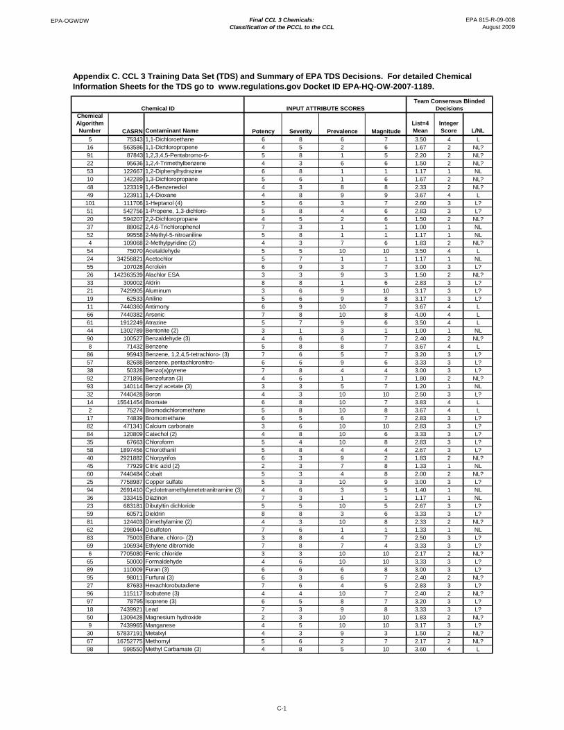
EPA-OGWDW Final CCL 3 Chemicals: EPA 815-R-09-008 Classification of the PCCL to the CCL August 2009
Appendix C. CCL 3 Training Data Set (TDS) and Summary of EPA TDS Decisions. For detailed Chemical Information Sheets for the TDS go to www.regulations.gov Docket ID EPA-HQ-OW-2007-1189.
Chemical ID INPUT ATTRIBUTE SCORES Team Consensus Blinded
Decisions Chemical Algorithm Number CASRN Contaminant Name Potency Severity Prevalence Magnitude
List=4 Mean
Integer Score L/NL
5 75343 1,1-Dichloroethane 6 8 6 7 3.50 4 L 16 563586 1,1-Dichloropropene 4 5 2 6 1.67 2 NL? 91 87843 1,2,3,4,5-Pentabromo-6- 5 8 1 5 2.20 2 NL? 22 95636 1,2,4-Trimethylbenzene 4 3 6 6 1.50 2 NL? 53 122667 1,2-Diphenylhydrazine 6 8 1 1 1.17 1 NL 10 142289 1,3-Dichloropropane 5 6 1 6 1.67 2 NL? 48 123319 1,4-Benzenediol 4 3 8 8 2.33 2 NL? 49 123911 1,4-Dioxane 4 8 9 9 3.67 4 L 101 111706 1-Heptanol (4) 5 6 3 7 2.60 3 L? 51 542756 1-Propene, 1,3-dichloro- 5 8 4 6 2.83 3 L? 20 594207 2,2-Dichloropropane 4 5 2 6 1.50 2 NL? 37 88062 2,4,6-Trichlorophenol 7 3 1 1 1.00 1 NL 52 99558 2-Methyl-5-nitroaniline 5 8 1 1 1.17 1 NL 4 109068 2-Methylpyridine (2) 4 3 7 6 1.83 2 NL?
54 75070 Acetaldehyde 5 5 10 10 3.50 4 L 24 34256821 Acetochlor 5 7 1 1 1.17 1 NL 55 107028 Acrolein 6 9 3 7 3.00 3 L? 26 142363539 Alachlor ESA 3 3 9 3 1.50 2 NL? 33 309002 Aldrin 8 8 1 6 2.83 3 L? 21 7429905 Aluminum 3 6 9 10 3.17 3 L? 19 62533 Aniline 5 6 9 8 3.17 3 L? 11 7440360 Antimony 6 9 10 7 3.67 4 L 66 7440382 Arsenic 7 8 10 8 4.00 4 L 61 1912249 Atrazine 5 7 9 6 3.50 4 L 44 1302789 Bentonite (2) 3 1 3 1 1.00 1 NL 90 100527 Benzaldehyde (3) 4 6 6 7 2.40 2 NL? 8 71432 Benzene 5 8 8 7 3.67 4 L
86 95943 Benzene, 1,2,4,5-tetrachloro- (3) 7 6 5 7 3.20 3 L? 57 82688 Benzene, pentachloronitro- 6 6 9 6 3.33 3 L? 38 50328 Benzo(a)pyrene 7 8 4 4 3.00 3 L? 92 271896 Benzofuran (3) 4 6 1 7 1.80 2 NL? 93 140114 Benzyl acetate (3) 3 3 5 7 1.20 1 NL 32 7440428 Boron 4 3 10 10 2.50 3 L? 14 15541454 Bromate 6 8 10 7 3.83 4 L 2 75274 Bromodichloromethane 5 8 10 8 3.67 4 L
17 74839 Bromomethane 6 5 6 7 2.83 3 L? 82 471341 Calcium carbonate 3 6 10 10 2.83 3 L? 84 120809 Catechol (2) 4 8 10 6 3.33 3 L? 35 67663 Chloroform 5 4 10 8 2.83 3 L? 58 1897456 Chlorothanil 5 8 4 4 2.67 3 L? 40 2921882 Chlorpyrifos 6 3 9 2 1.83 2 NL? 45 77929 Citric acid (2) 2 3 7 8 1.33 1 NL 60 7440484 Cobalt 5 3 4 8 2.00 2 NL? 25 7758987 Copper sulfate 5 3 10 9 3.00 3 L? 94 2691410 Cyclotetramethylenetetranitramine (3) 4 6 3 5 1.40 1 NL 36 333415 Diazinon 7 3 1 1 1.17 1 NL 23 683181 Dibutyltin dichloride 5 5 10 5 2.67 3 L? 59 60571 Dieldrin 8 8 3 6 3.33 3 L? 81 124403 Dimethylamine (2) 4 3 10 8 2.33 2 NL? 62 298044 Disulfoton 7 6 1 1 1.33 1 NL 83 75003 Ethane, chloro- (2) 3 8 4 7 2.50 3 L? 69 106934 Ethylene dibromide 7 8 7 4 3.33 3 L? 6 7705080 Ferric chloride 3 3 10 10 2.17 2 NL?
65 50000 Formaldehyde 4 6 10 10 3.33 3 L? 89 110009 Furan (3) 6 6 6 8 3.00 3 L? 95 98011 Furfural (3) 6 3 6 7 2.40 2 NL? 27 87683 Hexachlorobutadiene 7 6 4 5 2.83 3 L? 96 115117 Isobutene (3) 4 4 10 7 2.40 2 NL? 97 78795 Isoprene (3) 6 5 8 7 3.20 3 L? 18 7439921 Lead 7 3 9 8 3.33 3 L? 50 1309428 Magnesium hydroxide 2 3 10 10 1.83 2 NL? 9 7439965 Manganese 4 5 10 10 3.17 3 L?
30 57837191 Metalxyl 4 3 9 3 1.50 2 NL? 67 16752775 Methomyl 5 6 2 7 2.17 2 NL? 98 598550 Methyl Carbamate (3) 4 8 5 10 3.60 4 L
C-1

EPA-OGWDW Final CCL 3 Chemicals: EPA 815-R-09-008 Classification of the PCCL to the CCL August 2009
Chemical ID INPUT ATTRIBUTE SCORES Team Consensus Blinded
Decisions Chemical Algorithm Number CASRN Contaminant Name Potency Severity Prevalence Magnitude
List=4 Mean
Integer Score L/NL
99 12108133 Methylcyclopentadienylmanganese 7 9 5 8 3.80 4 L tricarbonyl(MMT) (3)
85 98851 Methylphenyl carbinol (3) 3 3 10 8 1.80 2 NL? 79 51218452 Metolachlor 4 3 6 7 1.83 2 NL? 41 21087649 Metribuzin 5 3 1 6 1.50 2 NL? 29 1634044 MTBE 4 5 5 8 2.33 2 NL? 42 91203 Naphthalene 5 3 7 6 2.00 2 NL? 56 14797558 Nitrate 3 3 10 10 2.00 2 NL? 28 14797650 Nitrite 4 3 10 9 2.50 3 L? 31 98953 Nitrobenzene 6 5 1 10 2.00 2 NL? 46 1836755 Nitrofen 5 8 1 5 2.17 2 NL? 68 100754 N-Nitrosopiperidine 7 8 1 1 1.67 2 NL? 1 109319 Nonanedioic acid, dihexyl ester (2) 2 7 1 1 1.00 1 NL
70 95487 o-cresol 4 6 1 1 1.00 1 NL 71 1910425 Paraquat 5 5 1 1 1.00 1 NL 78 56382 Parathion 5 3 2 3 1.17 1 NL 15 14797730 Perchlorate 8 7 9 8 4.00 4 L 100 77098 Phenolphthalein (3) 3 8 1 7 1.80 2 NL? 13 584087 Potassium carbonate 3 3 10 10 2.00 2 NL? 3 1610180 Prometon 5 7 1 1 1.17 1 NL
72 96184 Propane, 1,2,3-trichloro- 7 8 3 6 3.33 3 L? 88 106490 p-Toluidine (3) 6 8 5 8 3.60 4 L 73 91225 Quinoline 8 8 7 6 3.83 4 L 43 7440235 Sodium 4 4 10 10 2.83 3 L? 7 144558 Sodium bicarbonate 4 9 10 10 3.17 3 L?
74 96093 Styrene oxide 6 8 1 1 1.17 1 NL 39 14808798 Sulfate 4 3 10 10 2.50 3 L? 75 75650 tert-Butanol 3 3 10 8 1.83 2 NL? 34 127184 Tetrachloroethylene 5 8 9 7 3.67 4 L 76 78002 Tetraethyl lead 10 6 9 8 4.00 4 L 77 62566 Thiourea 4 7 7 5 2.67 3 L? 64 108883 Toluene 4 3 9 7 2.33 2 NL? 87 78422 Tri(ethylhexyl) phosphate (3) 4 6 3 5 1.80 2 NL? 102 102716 Triethanolamine (5) 4 8 8 7 3.00 3 L? 80 76879 Triphenyltin hydroxide 7 3 10 6 2.83 3 L? 47 1330207 Xylenes 4 3 9 7 2.17 2 NL? 12 7646857 Zinc chloride 4 3 10 9 2.50 3 L? 63 Synthetic 4 1 7 7 1.50 2 NL?
149 Synthetic 3 2 2 2 1.00 1 NL 150 Synthetic 5 3 1 2 1.00 1 NL 151 Synthetic 6 1 2 1 1.00 1 NL 152 Synthetic 2 8 1 1 1.00 1 NL 153 Synthetic 6 9 1 4 2.33 2 NL? 154 Synthetic 8 8 8 2 3.50 4 L 155 Synthetic 2 2 10 9 2.00 2 NL? 156 Synthetic 4 1 8 1 1.00 1 NL 157 Synthetic 7 3 8 3 2.00 2 NL? 158 Synthetic 4 8 8 1 2.33 2 NL? 159 Synthetic 10 8 8 1 3.50 4 L 160 Synthetic 1 3 5 9 1.33 1 NL 161 Synthetic 9 1 1 7 1.67 2 NL? 162 Synthetic 1 1 1 1 1.00 1 NL 163 Synthetic 2 6 1 9 1.83 2 NL? 164 Synthetic 7 8 4 7 3.67 4 L 165 Synthetic 4 5 10 9 3.17 3 L? 166 Synthetic 7 3 10 10 3.67 4 L 167 Synthetic 2 6 7 7 2.17 2 NL? 168 Synthetic 6 6 7 5 2.67 3 L? 169 Synthetic 10 9 10 7 4.00 4 L 170 Synthetic 5 1 5 3 1.00 1 NL 171 Synthetic 9 3 3 3 2.00 2 NL? 172 Synthetic 3 6 1 3 1.00 1 NL 173 Synthetic 8 7 1 2 2.33 2 NL? 174 Synthetic 10 5 1 1 2.00 2 NL? 175 Synthetic 8 8 8 8 4.00 4 L 176 Synthetic 1 5 10 3 1.33 1 NL 177 Synthetic 10 4 8 5 3.33 3 L? 178 Synthetic 3 8 10 1 1.83 2 NL? 179 Synthetic 10 8 9 4 3.83 4 L
C-2

EPA-OGWDW Final CCL 3 Chemicals: EPA 815-R-09-008 Classification of the PCCL to the CCL August 2009
Chemical ID INPUT ATTRIBUTE SCORES Team Consensus Blinded
Decisions Chemical Algorithm Number CASRN Contaminant Name Potency Severity Prevalence Magnitude
List=4 Mean
Integer Score L/NL
180 Synthetic 5 4 3 8 2.50 3 L? 181 Synthetic 2 2 10 7 1.17 1 NL 182 Synthetic 8 5 3 8 3.33 3 L? 183 Synthetic 1 8 5 10 2.83 3 L? 184 Synthetic 6 8 2 6 3.00 3 L? 185 Synthetic 1 2 9 8 1.33 1 NL 186 Synthetic 6 5 6 6 2.83 3 L? 187 Synthetic 8 8 8 6 3.83 4 L 188 Synthetic 1 8 7 7 2.17 2 NL? 189 Synthetic 9 8 7 10 4.00 4 L 190 Synthetic 5 4 3 3 1.17 1 NL 191 Synthetic 10 4 5 3 2.67 3 L? 192 Synthetic 5 6 3 5 2.17 2 NL? 193 Synthetic 9 8 9 9 4.00 4 L 194 Synthetic 6 6 1 1 1.17 1 NL 195 Synthetic 2 1 8 3 1.17 1 NL 196 Synthetic 6 2 8 2 1.50 2 NL? 197 Synthetic 3 7 6 3 2.17 2 NL? 198 Synthetic 6 8 8 1 2.83 3 L? 199 Synthetic 9 8 2 3 3.17 3 L? 200 Synthetic 3 1 1 6 1.17 1 NL 201 Synthetic 8 2 2 7 2.33 2 NL? 202 Synthetic 4 9 5 7 3.33 3 L? 203 Synthetic 8 8 1 7 3.50 4 L 204 Synthetic 3 5 6 8 2.33 2 NL? 205 Synthetic 9 8 9 4 3.67 4 L 206 Synthetic 10 2 1 1 1.50 2 NL? 207 Synthetic 8 4 6 9 3.33 3 L? 208 Synthetic 4 8 8 7 3.67 4 L 209 Synthetic 7 6 9 8 3.83 4 L 210 Synthetic 4 4 1 4 1.00 1 NL 211 Synthetic 9 3 4 3 2.33 2 NL? 212 Synthetic 7 7 7 7 3.50 4 L 213 Synthetic 4 7 3 5 2.17 2 NL? 214 Synthetic 7 8 1 4 2.67 3 L? 215 Synthetic 1 4 10 2 1.33 1 NL 216 Synthetic 6 3 10 5 2.50 3 L? 217 Synthetic 2 8 9 3 2.17 2 NL? 218 Synthetic 2 3 10 5 1.17 1 NL 219 Synthetic 8 8 6 5 3.67 4 L 220 Synthetic 5 3 3 10 2.50 3 L? 221 Synthetic 10 3 2 6 2.83 3 L? 222 Synthetic 5 8 2 6 2.67 3 L? 223 Synthetic 8 7 2 7 3.33 3 L? 224 Synthetic 7 7 9 4 3.67 4 L 225 Synthetic 2 4 6 9 2.33 2 NL? 226 Synthetic 8 3 10 6 3.50 4 L 227 Synthetic 1 8 7 8 2.33 2 NL? 228 Synthetic 10 8 6 8 3.83 4 L 229 Synthetic 4 4 4 2 1.00 1 NL 230 Synthetic 10 8 2 9 3.67 4 L 231 Synthetic 6 4 5 3 2.00 2 NL? 232 Synthetic 1 6 5 1 1.00 1 NL 233 Synthetic 7 6 4 2 2.00 2 NL? 234 Synthetic 2 3 10 4 1.00 1 NL 235 Synthetic 8 2 7 2 1.50 2 NL? 236 Synthetic 6 9 6 6 3.67 4 L 237 Synthetic 2 8 7 4 2.00 2 NL? 238 Synthetic 8 8 8 4 3.83 4 L 239 Synthetic 5 4 1 6 2.33 2 NL? 240 Synthetic 8 1 1 7 1.67 2 NL? 241 Synthetic 4 7 4 7 2.83 3 L? 242 Synthetic 10 8 10 3 3.83 4 L 243 Synthetic 9 7 4 6 3.83 4 L 244 Synthetic 4 1 8 9 2.00 2 NL? 245 Synthetic 7 2 10 6 2.67 3 L? 246 Synthetic 3 8 10 9 3.67 4 L 247 Synthetic 9 8 7 8 4.00 4 L 248 Synthetic 1 1 10 5 1.17 1 NL
C-3

EPA-OGWDW Final CCL 3 Chemicals: EPA 815-R-09-008 Classification of the PCCL to CCL August 2009
APPENDIX D. SOFTWARE SOURCES
Artificial Neural Networks – ANN methods packaged in R software libraries “MASS” and “nnet” are available at no charge from the website http://www.r-project.org, under the Free Software Foundation’s GNU General Public License.
Univariate Decision Tree – CART – methods packaged in the R software library “rpart” are available at no charge from the website http://www.r-project.org, under the Free Software Foundation’s GNU General Public License.
Multivariate Decision Tree – QUEST software is available at no charge from the website http://www.stat.wisc.edu/~loh/quest.html
Linear Modeling - Likelihood function was maximized using MathCAD’s built-in Maximize function (www.mathsoft.com).
Multivariate Adaptive Regression Splines – MARS methods packaged in the R software library “polspline” are available at no charge from the website http://www.r-project.org, under the Free Software Foundation’s GNU General Public License.
D - 1

EPA-OGWDW Final CCL 3 Chemicals: EPA 815-R-09-008 Classification of the PCCL to CCL August 2009
APPENDIX E. SOLUTIONS TO THE CLASSIFICATION MODELS USED IN THE CCL PROCESS
Artificial Neural Network – The software used does not reveal its decision rule. Instead, it provides classifications for contaminants that have been scored for the four attributes. When given a complete set of all possible combinations of integer attribute scores, the software provides classifications. Although not expressed mathematically, this complete description of the decision rule can be seen in Exhibit 4-4.
Example: Contaminant with scores (3, 4, 5, 6). Exhibit 29 shows this as a dark blue point. Not List.
Simple Linear Model – The maximum likelihood linear model is shown below. Y[i] is the estimated team-average classification and Pot[i], Sev[i], Prev[i], Mag[i] are the attribute scores for contaminant i. If Y[i] is less than 1.5, then the classification is Not List. Similarly, if Y[i] is at least 3.5, then the classification is List.
Y[i] = -1.671 + 0.241 * Pot[i] + 0.217 * Sev[i] + 0.116 * Prev[i] + 0.170 * Mag[i]
Example: Contaminant with scores (3, 4, 5, 6). Y = -1.671 + 0.241 * 3 + 0.217 * 4 + 0.116 * 5 + 0.170 * 6 = 1.520 Not List
Multivariate Tree (QUEST) – The solution involves a number of intermediate nodes and terminal nodes arranged as shown in Exhibit 4.1.1. When a contaminant encounters an intermediate node, a weighted sum of attribute scores is compared to a threshold value. The direction the contaminant moves from the node depends on whether the threshold is exceeded. Below, vector notation is used below to simplify the description. Letting X[i] be a column vector of attribute scores, (Pot[i], Sev[i], Prev[i], Mag[i]), then B1T*X[i] is the vector product of B1 (a column vector of weights) and X[i], which, in turn, is compared with the threshold. When the contaminant encounters a terminal node (Node 6, 10, 11, 16, 17, 29, 30, or 31), a classification is assigned.
Node 1: If B1*X[i] < 0.3023, then Node 2, otherwise Node 3. Node 2: If B2*X[i] < 0.3844, then Node 4, otherwise Node 5.
Node 4: If B4*X[i] < 0.6460, then Node 6, otherwise Node 7. Node 6: Not List Node 7: If B7*X[i] < 3.336, then Node 10, otherwise Node 11.
Node 10: Not List Node 11: Not List?
Node 5: If B5*X[i] < 1.213, then Node 16, otherwise Node 17. Node 16: Not List? Node 17: List?
Node 3: If B3*X[i] < 1.181, then Node 28, otherwise Node 29 Node 28: If B28*X[i] < 6.460, then Node 30, otherwise Node 31.
Node 30: List? Node 31: List
E-1

EPA-OGWDW Final CCL 3 Chemicals: EPA 815-R-09-008 Classification of the PCCL to CCL August 2009
Node 29: List
Exhibit A.1 – Tree Produced by QUEST (heavy arrows show path of contaminant with attribute scores 3, 4, 5, 6)
Exhibit A.2 - The column vectors of weights: B1 B2 B3 B4 B5 B7 B28
0.01631 0.01315 0.007523 0.01034
0.03008 0.02075 0.01214 0.02043
0.05223 0.06855 0.03516 0.01807
0.06890 0.01756 0.01753 0.05501
0.07779 0.06447 0.03300 0.04850
0.3531 0.1136 0.07560 0.2144
0.2966 0.3174 0.1995 0.1952
Example: Contaminant with scores X = (3, 4, 5, 6)
Node 1: B1 T*X = 0.01631*3 + 0.01315*4 + 0.007523*5 + 0.01034*6 = 0.2012 This is less than 0.3023, so go to Node 2.
Node 2: B2 T*X = 0.03008*3 + 0.02075*4 + 0.01214*5 + 0.02043*6 = 0.3565 This is less than 0.3844, so go to Node 4.
E-2
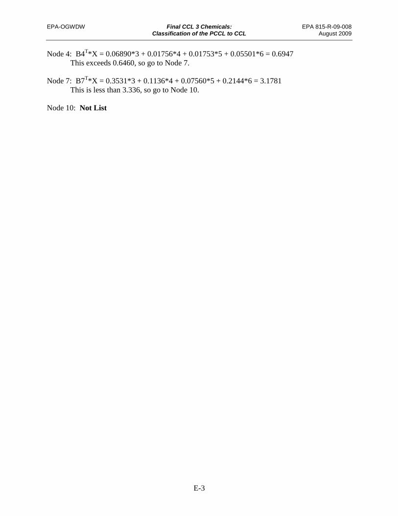
EPA-OGWDW Final CCL 3 Chemicals: EPA 815-R-09-008 Classification of the PCCL to CCL August 2009
Node 4: B4T*X = 0.06890*3 + 0.01756*4 + 0.01753*5 + 0.05501*6 = 0.6947 This exceeds 0.6460, so go to Node 7.
Node 7: B7T*X = 0.3531*3 + 0.1136*4 + 0.07560*5 + 0.2144*6 = 3.1781 This is less than 3.336, so go to Node 10.
Node 10: Not List
E-3

EPA-OGWDW Final CCL 3 Chemicals: EPA 815-R-09-008 Classification of the PCCL to CCL August 2009
Appendix F. Chemicals Reviewed by the EPA Evaluation Team: Summary of Results Set 1 Summary Direction - disagree Overall Confidence POTENCY Data Element PREVALENCE Data Element
CASRN Common Name Model Decision
# Evaluators
% agreement
+/- (+ toward
L)
Value (L=4; NL=1)
Category H% M% L% Value H=3; L=1)
Element (L4G) Source
Type (NCAR /
CAR) Element (L4G) Source
51285 2,4-Dinitrophenol NL 18 100 +/-0 1.00 NL 65% 35% 0% 2.647 Reference Dose (RfD)
IRIS NCAR Percentage of PWSs (Detects), All Water, Finished
UCMR
60571 Dieldrin L? - L 18 83 +7 3.66 L 41% 47% 12% 2.294 Lifetime Cancer Risk (10^-4)
IRIS CAR Percentage of PWSs (Detects), All Water, Finished
NCODR1 2
62737 Dichlorvos NL - NL? 16 88 -1 1.63 NL? 33% 53% 13% 2.200 Lifetime Cancer Risk (10^-4)
IRIS CAR Percentage of Samples (Detects), Surface Water, Ambient
NREC
63252 Carbaryl NL? 16 69 +/-0 2.00 NL? 33% 47% 20% 2.133 Reference Dose (RfD)
OPP NCAR Percentage of PWSs (Detects), All Water, Finished
NCODR1 2
67641 Acetone L? 18 78 -2 2.75 L? 40% 60% 0% 2.400 Reference Dose (RfD)
IRIS NCAR Percentage of Sites (Detects), All Water, Ambient
NAWQA
67721 Hexachloroethane NL 17 100 +1 1.06 NL 44% 56% 0% 2.438 Reference Dose (RfD)
IRIS NCAR Percentage of Sites (Detects), All Water, Ambient
NAWQA
72559 p,p'-DDE NL - NL? 16 88 +1 1.61 NL? 40% 53% 7% 2.333 Lifetime Cancer Risk (10^-4)
IRIS CAR Percentage of PWSs (Detects), All Water, Finished
UCMR
74839 Methyl bromide Bromomethane
L? 17 82 +3 3.11 L? 47% 47% 7% 2.400 Reference Dose (RfD)
IRIS NCAR Percentage of PWSs (Detects), All Water, Finished
NCODR1 2
74873 Chloromethane (Methyl chloride)
L? 16 81 +/-0 2.88 L? 50% 50% 0% 2.500 Reference Dose (RfD)
EPAHA NCAR Percentage of PWSs (Detects), All Water, Finished
NCODR1 2
74953 Dibromomethane NL? 14 71 -1 1.92 NL? 36% 57% 7% 2.286 Reference Dose (RfD)
RAISH E
NCAR Percentage of PWSs (Detects), All Water, Finished
NCODR1 2
74975 Halon 1011 (bromochloromethan e)
NL? 13 62 -2 1.83 NL? 40% 60% 0% 2.400 Reference Dose (RfD)
EPAHA NCAR Percentage of PWSs (Detects), All Water, Finished
NCODR1 2
75150 Carbon disulfide NL? - L? 15 53 -2 2.21 NL? 29% 64% 7% 2.214 Reference Dose (RfD)
IRIS NCAR Percentage of Sites (Detects), All Water, Ambient
NAWQA
75343 1,1-Dichloroethane L? 12 67 +1 3.00 L? 18% 64% 18% 2.000 Slope Factor (Oral)
OEHHA CAR Percentage of PWSs (Detects), All Water, Finished
NCODR1 2
75694 CFC-11. Trichlorofluoromethan e
L? - L 13 69 +1 3.38 L? 42% 50% 8% 2.333 Reference Dose (RfD)
IRIS NCAR Percentage of PWSs (Detects), All Water, Finished
NCODR1 2
75718 CFC-12. Dichlorofluoromethan e
NL? 13 77 -4 1.71 NL? 50% 42% 8% 2.417 Reference Dose (RfD)
IRIS NCAR Percentage of PWSs (Detects), All Water, Finished
NCODR1 2
F-1

EPA-OGWDW Final CCL 3 Chemicals: EPA 815-R-09-008 Classification of the PCCL to CCL August 2009
Appendix F. Chemicals Reviewed by the EPA Evaluation Team: Summary of Results Set 1 Summary Direction - disagree Overall Confidence POTENCY Data Element PREVALENCE Data Element
CASRN Common Name Model Decision
# Evaluators
% agreement
+/- (+ toward
L)
Value (L=4; NL=1)
Category H% M% L% Value H=3; L=1)
Element (L4G) Source
Type (NCAR /
CAR) Element (L4G) Source
79345 1,1,2,2-Tetrachloroethane
NL? 14 64 +1 2.04 NL? 36% 55% 9% 2.273 Reference Dose (RfD)
EPAHA NCAR Percentage of PWSs (Detects), All Water, Finished
NCODR1 2
80626 Methyl methacrylate NL 13 100 +/-0 1.00 NL 58% 42% 0% 2.583 Reference Dose (RfD)
IRIS NCAR Percentage of Sites (Detects), All Water, Ambient
NAWQA
86500 Azinphos-methyl NL? 12 100 +1 2.15 NL? 27% 64% 9% 2.182 Reference Dose (RfD)
OPP NCAR Percentage of Sites (Detects), All Water, Ambient
NAWQA
87616 1,2,3-Trichlorobenzene
NL - NL? 13 77 -3 1.47 NL 42% 42% 17% 2.250 Lowest Observed Adverse Effect Level (LOAEL)
RTECS NCAR Percentage of PWSs (Detects), All Water, Finished
NCODR1 2
87683 Hexachlorobutadiene L? 13 77 -2 2.75 L? 46% 46% 8% 2.385 Reference Dose (RfD)
EPAHA NCAR Percentage of PWSs (Detects), All Water, Finished
NCODR1 2
88062 2,4,6-Trichlorophenol NL 13 92 +1 1.08 NL 42% 50% 8% 2.333 Reference Dose (RfD)
EPAHA NCAR Percentage of PWSs (Detects), All Water, Finished
UCMR
91203 Naphthalene NL? 13 85 -1 1.93 NL? 67% 33% 0% 2.667 Reference Dose (RfD)
IRIS NCAR Percentage of PWSs (Detects), All Water, Finished
NCODR1 2
94746 MCPA NL? - L? 14 71 -1 2.38 NL? 33% 42% 25% 2.083 Reference Dose (RfD)
OPP NCAR Percentage of Sites (Detects), All Water, Ambient
NAWQA
95498 o-Chlorotoluene NL? 13 77 -4 1.71 NL? 58% 42% 0% 2.583 Reference Dose (RfD)
IRIS NCAR Percentage of PWSs (Detects), All Water, Finished
NCODR1 2
95636 1,2,4-Trimethylbenzene
NL? 13 69 -1 1.92 NL? 33% 33% 33% 2.000 Reference Dose (RfD)
RAISH E
NCAR Percentage of PWSs (Detects), All Water, Finished
NCODR1 2
F-2

EPA-OGWDW Final CCL 3 Chemicals: EPA 815-R-09-008 Classification of the PCCL to CCL August 2009
Appendix F. Chemicals Reviewed by the EPA Evaluation Team: Summary of Results
Set 2 Summary Direction - disagree Overall Confidence POTENCY Data Element PREVALENCE Data Element
CASRN Common Name Model Decision
# Evaluator
s
% agreement
+/- (+ toward
L)
Value (L=4; NL=1)
Categor y H% M% L% Value
H=3; L=1) Element
(L4G) Source Type
(NCAR / CAR)
Element (L4G) Source
2212671 Molinate L? 19 84 -1 3 L? 32% 58% 11% 2.211 Reference Dose (RfD)
IRIS NCAR Percentage of PWSs (Detects), All Water, Finished
UCMR
2312358 Propargite L? 18 72 -5 3 L? 24% 59% 18% 2.059 Reference Dose (RfD)
OPP NCAR Percentage of Sites (Detects), All Water, Ambient
NAWQA
5989275 (D)-Limonene NL? 17 82 -4 2 NL? 24% 59% 18% 2.059 No Observed Effect Level (NOEL)
NTP NCAR Percentage of Samples (Detects), Surface Water, Ambient
NREC
7439987 Molybdenum L? - L 18 78 +/-0 3 L? 50% 39% 11% 2.389 UL IOM NCAR Percentage of Samples (Detects), All Water, Finished
NIRS
7440020 Nickel L? 18 89 -2 3 L? 28% 67% 6% 2.222 Reference Dose (RfD)
IRIS NCAR Percentage of Samples (Detects), All Water, Finished
NIRS
7440097 Potassium L? 18 44 -9 2 NL? 24% 24% 53% 1.706 Lowest Observed Adverse Effect Level (LOAEL)
NAS NCAR Percentage of Samples (Detects), All Water, Finished
NIRS
7440213 Silicon L 18 61 -4 3 L? 17% 33% 50% 1.667 Lethal Dose 50 (LD50)
RTECS NCAR Percentage of Samples (Detects), All Water, Finished
NIRS
7440235 Sodium L? 19 68 -3 3 L? 26% 37% 37% 1.895 Lowest Observed Adverse Effect Level (LOAEL)
RTECS NCAR Percentage of Samples (Detects), All Water, Finished
NIRS
7440246 Strontium L? 19 74 +/-0 3 L? 26% 47% 26% 2.000 Reference Dose (RfD)
IRIS NCAR Percentage of Samples (Detects), All Water, Finished
NIRS
7440428 Boron L? 18 61 +3 3 L? 24% 53% 24% 2.000 Reference Dose (RfD)
IRIS NCAR Percentage of Samples (Detects), All Water, Finished
NIRS
7440484 Cobalt NL? - L? 17 71 -1 2 NL? 24% 53% 24% 2.000 MRL-Int ATSDR NCAR Percentage of Samples (Detects), All Water, Finished
NIRS
7440564 Germanium L? 18 61 -2 3 L? 18% 24% 59% 1.588 Lowest Observed Adverse Effect Level (LOAEL)
RTECS NCAR Percentage of Samples (Detects), All Water, Finished
NIRS
F-3

EPA-OGWDW Final CCL 3 Chemicals: EPA 815-R-09-008 Classification of the PCCL to CCL August 2009
Appendix F. Chemicals Reviewed by the EPA Evaluation Team: Summary of Results
Set 2 Summary Direction - disagree Overall Confidence POTENCY Data Element PREVALENCE Data Element
CASRN Common Name Model Decision
# Evaluator
s
% agreement
+/- (+ toward
L)
Value (L=4; NL=1)
Categor y H% M% L% Value
H=3; L=1) Element
(L4G) Source Type
(NCAR / CAR)
Element (L4G) Source
7440622 Vanadium L? - L 18 78 -4 3 L? 18% 59% 24% 1.941 MRL-Int ATSDR NCAR Percentage of Samples (Detects), All Water, Finished
NIRS
7664417 Ammonia NL? 17 82 -4 2 NL? 24% 65% 12% 2.118 Reference Dose (RfD)
RAISHE NCAR Percentage of Sites (Detects), All Water, Ambient
NAWQA
7723140 White Phosphorus L 19 100 -1 4 L 63% 32% 5% 2.579 Reference Dose (RfD)
IRIS NCAR Percentage of Samples (Detects), All Water, Finished
NIRS
13071799 Terbufos NL 17 82 +3 1 NL 63% 31% 6% 2.563 Reference Dose (RfD)
OPP NCAR Percentage of PWSs (Detects), All Water, Finished
UCMR
13194484 Ethoprop NL? 16 81 +2 2 NL? 33% 39% 28% 2.056 Reference Dose (RfD)
OPP NCAR Percentage of Sites (Detects), All Water, Ambient
NAWQA
13494809 Tellurium NL? - L? 16 56 +2 2 NL? 18% 18% 65% 1.529 NOAEL Journal NCAR Percentage of Samples (Detects), All Water, Finished
NIRS
14797730 Perchlorate NL? - L? 16 50 +6 3 L? 33% 47% 20% 2.133 Reference Dose (RfD)
IRIS NCAR Percentage of PWSs (Detects), All Water, Finished
UCMR
16655826 3-Hydroxycarbofuran L? 18 83 +2 3 L? 29% 53% 18% 2.118 RfD OPP NCAR Percentage of PWSs (Detects), All Water, Finished
NCODR12
16752775 Methomyl NL? 16 56 -1 2 NL? 27% 67% 7% 2.200 Reference Dose (RfD)
OPP NCAR Percentage of PWSs (Detects), All Water, Finished
NCODR12
21087649 Metribuzin NL - NL? 16 69 +/-0 2 NL? 50% 31% 19% 2.313 Reference Dose (RfD)
OPP NCAR Percentage of PWSs (Detects), All Water, Finished
NCODR12
21725462 Cyanazine NL? 17 65 +/-0 2 NL? 31% 63% 6% 2.250 Reference Dose (RfD)
EPAHA NCAR Percentage of Sites (Detects), All Water, Ambient
NAWQA
25013165 Butylated hydroxyanisole NL? 15 73 +/-0 2 NL? 13% 40% 47% 1.667 Lowest Observed Adverse Effect Level (LOAEL)
RTECS NCAR Percentage of Samples (Detects), Surface Water, Ambient
NREC
25057890 Bentazon NL? 15 53 +1 2 NL? 36% 57% 7% 2.286 Reference Dose (RfD)
IRIS NCAR Percentage of Sites (Detects), All Water, Ambient
NAWQA
27314132 Norflurazon NL? 14 79 +2 2 NL? 31% 46% 23% 2.077 Reference Dose (RfD)
OPP NCAR Percentage of Sites (Detects), All Water, Ambient
NAWQA
F-4

EPA-OGWDW Final CCL 3 Chemicals: EPA 815-R-09-008 Classification of the PCCL to CCL August 2009
Appendix F. Chemicals Reviewed by the EPA Evaluation Team: Summary of Results
Set 2 Summary Direction - disagree Overall Confidence POTENCY Data Element PREVALENCE Data Element
CASRN Common Name Model Decision
# Evaluator
s
% agreement
+/- (+ toward
L)
Value (L=4; NL=1)
Categor y H% M% L% Value
H=3; L=1) Element
(L4G) Source Type
(NCAR / CAR)
Element (L4G) Source
34014181 Tebuthiuron NL - NL? 15 73 -4 1 NL 53% 33% 13% 2.400 Reference Dose (RfD)
OPP NCAR Percentage of Sites (Detects), All Water, Ambient
NAWQA
34256821 Acetochlor NL 16 69 +4 1 NL 67% 20% 13% 2.533 Reference Dose (RfD)
IRIS NCAR Percentage of PWSs (Detects), All Water, Finished
UCMR
51218452 Metolachlor NL? 13 69 -3 2 NL? 38% 54% 8% 2.308 Reference Dose (RfD)
OPP NCAR Percentage of PWSs (Detects), All Water, Finished
NCODR12
F-5

EPA-OGWDW Final CCL 3 Chemicals: EPA 815-R-09-008 Classification of the PCCL to CCL August 2009
Appendix F. Chemicals Reviewed by the EPA Evaluation Team: Summary of Results Set 3 Summary Direction - disagree Overall Confidence
POTENCY Data Element PREVALENCE Data Element
CASRN Common Name Model Decision
# Evaluators
% agreement
+/- (+ toward L)
Value (L=4; NL=1)
Category H% M% L% Value H=3; L=1)
Element (L4G) Source
Type (NCAR /
CAR) Element (L4G) Source
96184 1,2,3-Trichloropropane NL? 16 75 +1 2.12 NL? 44% 31% 25% 2.188 Reference Dose (RfD)
IRIS NCAR Percentage of PWSs (Detects), All Water, Finished
NCODR12
96333 Methyl acrylate NL 15 93 +1 1.07 NL 40% 53% 7% 2.333 Reference Dose (RfD)
RAISHE NCAR Percentage of Sites (Detects), All Water, Ambient
NAWQA
98066 tert-Butylbenzene NL? 16 75 -1 1.97 NL? 19% 69% 13% 2.063 Lowest Observed Adverse Effect Level (LOAEL)
RTECS NCAR Percentage of PWSs (Detects), All Water, Finished
NCODR12
98953 Nitrobenzene NL?-L? 16 44 +5 2.75 L? 31% 38% 31% 2.000 Reference Dose (RfD)
IRIS NCAR Percentage of PWSs (Detects), All Water, Finished
UCMR
103651 n-Propylbenzene NL? 16 94 +1 2.03 NL? 31% 50% 19% 2.125 Lowest Observed Adverse Effect Level (LOAEL)
RTECS NCAR Percentage of PWSs (Detects), All Water, Finished
NCODR12
106434 p-Chlorotoluene NL? 15 87 -1 1.94 NL? 31% 56% 13% 2.188 Reference Dose (RfD)
EPAHA / IRIS
NCAR Percentage of PWSs (Detects), All Water, Finished
NCODR12
107028 Acrolein L?-L 16 69 +1 3.53 L 25% 63% 13% 2.125 Reference Dose (RfD)
RAISHE NCAR Percentage of Sites (Detects), All Water, Ambient
NAWQA
107131 Acrylonitrile NL?-NL 15 73 +3 1.78 NL? 20% 73% 7% 2.133 Lifetime Cancer Risk (10^-4)
EPAHA CAR Percentage of Sites (Detects), All Water, Ambient
NAWQA
108054 Vinyl acetate NL 15 100 +/- 0 1.00 NL 40% 47% 13% 2.267 Reference Dose (RfD)
RAISHE NCAR Percentage of Sites (Detects), All Water, Ambient
NAWQA
108861 Bromobenzene NL? 16 69 +3 2.09 NL? 27% 53% 20% 2.067 Reference Dose (RfD)
RAISHE NCAR Percentage of PWSs (Detects), All Water, Finished
NCODR12
109999 Tetrahydrofuran L? 16 75 -1 2.93 L? 13% 47% 40% 1.733 No Observed Effect Level (NOEL)
Journal NCAR Percentage of Sites (Detects), All Water, Ambient
NAWQA
115968 Trichlorethyl phosphate NL?-L? 14 50 -3 2.39 NL? 7% 60% 33% 1.733 Reference Dose (RfD)
RAISHE NCAR Percentage of Samples (Detects), Surface Water, Ambient
NREC
121142 2,4-Dinitrotoluene L?-L 15 60 +1 3.53 L 38% 54% 8% 2.308 Lifetime Cancer Risk (10^-4)
EPAHA CAR Percentage of PWSs (Detects), All Water, Finished
UCMR
F-6
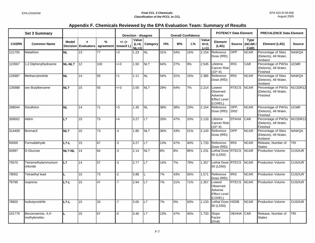
EPA-OGWDW Final CCL 3 Chemicals: EPA 815-R-09-008 Classification of the PCCL to CCL August 2009
Appendix F. Chemicals Reviewed by the EPA Evaluation Team: Summary of Results Set 3 Summary Direction - disagree Overall Confidence
POTENCY Data Element PREVALENCE Data Element
CASRN Common Name Model Decision
# Evaluators
% agreement
+/- (+ toward L)
Value (L=4; NL=1)
Category H% M% L% Value H=3; L=1)
Element (L4G) Source
Type (NCAR /
CAR) Element (L4G) Source
121755 Malathion NL 13 77 +3 1.23 NL 31% 54% 15% 2.154 Reference Dose (RfD)
OPP NCAR Percentage of Sites (Detects), All Water, Ambient
NAWQA
122667 1,2-Diphenylhydrazine NL-NL? 12 100 +/-0 1.50 NL? 64% 27% 9% 2.545 Lifetime Cancer Risk (10^-4)
IRIS CAR Percentage of PWSs (Detects), All Water, Finished
UCMR
126987 Methacrylonitrile NL 14 93 +1 1.11 NL 54% 31% 15% 2.385 Reference Dose (RfD)
IRIS NCAR Percentage of Sites (Detects), All Water, Ambient
NAWQA
135988 sec-Butylbenzene NL? 15 93 +/-0 2.00 NL? 29% 64% 7% 2.214 Lowest Observed Adverse Effect Level (LOAEL)
RTECS NCAR Percentage of PWSs (Detects), All Water, Finished
NCODR12
298044 Disulfoton NL 14 71 +3 1.35 NL 38% 38% 23% 2.154 Reference Dose (RfD)
OPP, 2002
NCAR Percentage of PWSs (Detects), All Water, Finished
UCMR
309002 Aldrin L? 15 73 +4 3.27 L? 33% 47% 20% 2.133 Lifetime Cancer Risk (10^-4)
EPAHA CAR Percentage of PWSs (Detects), All Water, Finished
NCODR12
314409 Bromacil NL? 15 73 -4 1.80 NL? 36% 43% 21% 2.143 Reference Dose (RfD)
OPP NCAR Percentage of Sites (Detects), All Water, Ambient
NAWQA
50000 Formaldehyde L?-L 15 67 -3 3.27 L? 13% 47% 40% 1.733 Reference Dose (RfD)
IRIS NCAR Release, Number of States
TRI
50997 D-Glucose NL?-NL 14 64 -3 2.14 NL? 8% 8% 85% 1.231 Lethal Dose 50 (LD50)
RTECS NCAR Production Volume CUS/IUR
75570 Tetramethylammonium chloride
L? 14 57 -3 2.77 L? 14% 7% 79% 1.357 Lethal Dose 50 (LD50)
RTECS NCAR Production Volume CUS/IUR
78002 Tetraethyl lead L 15 73 -2 3.88 L 7% 43% 50% 1.571 Reference Dose (RfD)
IRIS NCAR Production Volume CUS/IUR
78795 Isoprene L?-L 15 47 -7 2.94 L? 7% 21% 71% 1.357 Lowest Observed Adverse Effect Level (LOAEL)
RTECS NCAR Production Volume CUS/IUR
78820 Isobutyronitrile L?-L 15 33 -7 3.00 L? 7% 0% 93% 1.133 Lethal Dose 50 (LD50)
HSDB NCAR Production Volume CUS/IUR
101779 Benzenamine, 4,4'-methylenebis-
L 15 67 -5 3.40 L? 13% 47% 40% 1.733 Slope Factor (Oral)
OEHHA CAR Release, Number of States
TRI
F-7

EPA-OGWDW Final CCL 3 Chemicals: EPA 815-R-09-008 Classification of the PCCL to CCL August 2009
Appendix F. Chemicals Reviewed by the EPA Evaluation Team: Summary of Results Set 3 Summary Direction - disagree Overall Confidence
POTENCY Data Element PREVALENCE Data Element
CASRN Common Name Model Decision
# Evaluators
% agreement
+/- (+ toward L)
Value (L=4; NL=1)
Category H% M% L% Value H=3; L=1)
Element (L4G) Source
Type (NCAR /
CAR) Element (L4G) Source
108930 Cyclohexanol L?-L 14 64 -6 2.83 L? 7% 21% 71% 1.357 Lethal Dose 50 (LD50)
RTECS NCAR Release, Number of States
TRI
302012 Hydrazine L 15 87 -1 3.79 L 13% 53% 33% 1.800 Lifetime Cancer Risk (10^-4)
IRIS CAR Release, Number of States
TRI
625558 Isopropyl formate L 13 54 -5 3.46 L? 0% 7% 93% 1.071 Lethal Dose 50 (LD50)
RTECS NCAR Production Volume CUS/IUR
1111780 Ammonium carbamate L? 13 77 -2 2.75 L? 14% 7% 79% 1.357 Lethal Dose 50 (LD50)
RTECS NCAR Production Volume CUS/IUR
1335326 Lead acetate L 14 50 -6 3.35 L? 8% 17% 75% 1.333 Slope Factor (Oral)
OEHHA CAR Production Volume CUS/IUR
3268493 Methional L? 13 69 -2 2.86 L? 0% 31% 69% 1.308 Lethal Dose 50 (LD50)
RTECS NCAR Production Volume CUS/IUR
4719044 Hexahydro-1,3,5-tris(2-hydroxyethyl)-s-triazine
L 13 38 -6 3.41 L? 7% 7% 86% 1.214 Lethal Dose 50 (LD50)
RTECS NCAR Production Volume CUS/IUR
5216251 4-Chlorobenzotrichloride L?-L 14 86 -2 3.21 L? 14% 36% 50% 1.643 NOAEL OPPT NCAR Production Volume CUS/IUR 6610293 Methylthiosemicarbazide L? 14 71 -2 2.75 L? 0% 15% 85% 1.154 Lethal Dose
50 (LD50) RTECS NCAR Production Volume CUS/IUR
13463406 Iron pentacarbonyl L?-L 13 62 -6 2.81 L? 0% 31% 69% 1.308 Lethal Dose 50 (LD50)
HSDB NCAR Release, Number of States
TRI
23422539 Methanimidamide, N,N-dimethyl-N'-[3-[[(methylamino)carbonyl]o xy]phenyl]-, monohydrochloride
L?-L 14 57 -3 3.27 L? 17% 42% 42% 1.750 Reference Dose (RfD)
OPP NCAR Release, Number of States
NCFAP
71751412 Avermectin B1 L?-L 13 69 -1 3.39 L? 14% 29% 57% 1.571 ADI JMPR 1997
NCAR Release, Number of States
NCFAP
91465086 Cyclopropanecarboxylic acid, 3-2-chloro-3,3,3-trifluoro-1-propenyl)-2,2-dimethyl- cyano(3-phenoxyphenyl)methyl ester, 1.alpha.(S*),3.alpha.(Z)-(.+ -.)-
L?-L 14 71 -4 3.11 L? 14% 36% 50% 1.643 Reference Dose (RfD)
IRIS NCAR Release, Number of States
NCFAP
F-8

EPA-OGWDW Final CCL 3 Chemicals: EPA 815-R-09-008 Classification of the PCCL to CCL August 2009
Appendix F. Chemicals Reviewed by the EPA Evaluation Team: Summary of Results Set 4 Summary Direction - disagree Overall Confidence POTENCY Data Element PREVALENCE Data
Element
CASRN Common Name Model Decision
# Evaluators
% agreement
+/- (+ toward L)
Value (L=4; NL=1)
Category H% M% L% Value H=3; L=1)
Element (L4G) Source Type
(NCAR / CAR)
Element (L4G) Source
Cobalt compounds L 8 75 -2 3.81 L 22% 22% 56% 1.667 Lowest Observed Adverse Effect Level (LOAEL)
Journal NCAR Release, Number of States
TRI
51796 Urethane L 8 63 -2 3.79 L 22% 0% 78% 1.444 No Observed Effect Level (NOEL)
Journal NCAR Release, Number of States
TRI
55630 Nitroglycerin L? - L 9 78 +/- 0 3.50 L 9% 18% 73% 1.364 Lowest Observed Adverse Effect Level (LOAEL)
RTECS NCAR Release, Number of States
TRI
60355 Acetamide L 9 67 -2 3.56 L 20% 20% 60% 1.600 Slope Factor (Oral)
OEHHA CAR Release, Number of States
TRI
62533 Aniline L? - L 10 70 +2 3.61 L 20% 30% 50% 1.700 Reference Dose (RfD)
RAISHE NCAR Release, Number of States
TRI
67561 Methanol L? - L 10 60 +1 3.45 L? 17% 50% 33% 1.833 Reference Dose (RfD)
IRIS NCAR Release, Number of States
TRI
71363 1-Butanol L? - L 11 55 -1 3.33 L? 17% 33% 50% 1.667 Reference Dose (RfD)
IRIS NCAR Release, Number of States
TRI
75218 Ethylene oxide L 9 78 -2 3.78 L 36% 18% 45% 1.909 Slope Factor (Oral)
OEHHA CAR Release, Number of States
TRI
75569 Propylene oxide L 9 89 -1 3.78 L 36% 18% 45% 1.909 Slope Factor (Oral)
OPP CAR Release, Number of States
TRI
76879 Triphenyltin hydroxide L 10 80 -2 3.90 L 22% 44% 33% 1.889 Slope Factor (Oral)
OPP CAR Release, Number of States
NCFAP
80159 Cumene hydroperoxide L 10 60 -3 3.61 L 18% 9% 73% 1.455 Lowest Observed Adverse Effect Level (LOAEL)
RTECS NCAR Release, Number of States
TRI
106990 1,3-Butadiene L 11 73 -2 3.80 L 27% 9% 64% 1.636 Slope Factor (Oral)
OEHHA CAR Release, Number of States
TRI
107211 Ethylene glycol L 10 80 -2 3.70 L 27% 36% 36% 1.909 Reference Dose (RfD)
IRIS NCAR Release, Number of States
TRI
109864 2-Methoxyethanol L 9 78 -3 3.65 L 30% 10% 60% 1.700 Reference Dose (RfD)
RAISHE NCAR Release, Number of States
TRI
121448 Triethylamine L 7 43 -4 3.36 L? 0% 29% 71% 1.286 Lowest Observed Adverse Effect Level (LOAEL)
RTECS NCAR Release, Number of States
TRI
F-9

EPA-OGWDW Final CCL 3 Chemicals: EPA 815-R-09-008 Classification of the PCCL to CCL August 2009
Appendix F. Chemicals Reviewed by the EPA Evaluation Team: Summary of Results Set 4 Summary Direction - disagree Overall Confidence POTENCY Data Element PREVALENCE Data
Element
CASRN Common Name Model Decision
# Evaluators
% agreement
+/- (+ toward L)
Value (L=4; NL=1)
Category H% M% L% Value H=3; L=1)
Element (L4G) Source Type
(NCAR / CAR)
Element (L4G) Source
123911 1,4-Dioxane L 9 100 +/-0 4.00 L 30% 30% 40% 1.900 Lifetime Cancer Risk (10^-4)
EPAHA CAR Release, Number of States
TRI
133062 Captan L 10 70 -2 3.72 L 33% 22% 44% 1.889 Slope Factor (Oral)
OPP CAR Release, Number of States
NCFAP
137304 Ziram L 8 88 -1 3.75 L 13% 25% 63% 1.500 Slope Factor (Oral)
OPP CAR Release, Number of States
NCFAP
319846 .alpha.-Hexachlorocyclohexane
L? 12 67 +1 3.00 L? 18% 64% 18% 2.000 Lifetime Cancer Risk (10^-4)
IRIS CAR Percentage of Sites (Detects), All Water, Ambient
NAWQA
330541 Diuron NL? 13 77 +3 2.19 NL? 18% 64% 18% 2.000 Reference Dose (RfD)
OPP NCAR Percentage of PWSs (Detects), All Water, Finished
UCMR
330552 Linuron NL 12 92 +/-0 1.00 NL 50% 40% 10% 2.400 Reference Dose (RfD)
OPP NCAR Percentage of PWSs (Detects), All Water, Finished
UCMR
333415 Diazinon NL 11 91 +1 1.09 NL 45% 36% 18% 2.273 Reference Dose (RfD)
OPP NCAR Percentage of PWSs (Detects), All Water, Finished
UCMR
541731 m-Dichlorobenzene NL? 13 77 +1 2.00 NL? 45% 45% 9% 2.364 Reference Dose (RfD)
EPAHA NCAR Percentage of PWSs (Detects), All Water, Finished
NCODR12
542756 Telone L? 13 62 +3 3.23 L? 25% 50% 25% 2.000 Slope Factor (Oral)
OPP CAR Percentage of PWSs (Detects), All Water, Finished
NCODR12
630206 1,1,1,2-Tetrachloroethane L? 13 77 -1 2.88 L? 27% 64% 9% 2.182 Lifetime Cancer Risk (10^-4)
EPAHA CAR Percentage of PWSs (Detects), All Water, Finished
NCODR12
F-10

EPA-OGWDW Final CCL 3 Chemicals: EPA 815-R-09-008 Classification of the PCCL to CCL August 2009
Appendix F. Chemicals Reviewed by the EPA Evaluation Team: Summary of Results Set 4 Summary Direction - disagree Overall Confidence POTENCY Data Element PREVALENCE Data
Element
CASRN Common Name Model Decision
# Evaluators
% agreement
+/- (+ toward L)
Value (L=4; NL=1)
Category H% M% L% Value H=3; L=1)
Element (L4G) Source Type
(NCAR / CAR)
Element (L4G) Source
759944 S-Ethyl dipropylthiocarbamate
NL 12 75 +3 1.38 NL 55% 45% 0% 2.545 Reference Dose (RfD)
IRIS NCAR Percentage of PWSs (Detects), All Water, Finished
UCMR
944229 Fonofos NL 12 83 +/-0 1.00 NL 60% 40% 0% 2.600 Reference Dose (RfD)
IRIS NCAR Percentage of PWSs (Detects), All Water, Finished
UCMR
1313275 Molybdenum oxide (MoO3)
L 11 45 -3 3.38 L? 0% 25% 75% 1.250 RfD (UL) DRI NCAR Release, Number of States
TRI
1582098 Trifluralin NL - NL? 11 82 +2 1.59 NL? 56% 44% 0% 2.556 Reference Dose (RfD)
OPP NCAR Percentage of Sites (Detects), All Water, Ambient
NAWQA
1610180 Prometon NL 12 100 +/-0 1.00 NL 40% 40% 20% 2.200 Reference Dose (RfD)
IRIS NCAR Percentage of PWSs (Detects), All Water, Finished
UCMR
1634044 Methyl tert-butyl ether L? 12 58 +5 3.42 L? 10% 70% 20% 1.900 Slope Factor (Oral)
OEHHA CAR Percentage of PWSs (Detects), All Water, Finished
UCMR
1861321 Chlorthal-dimethyl (Dacthal)
NL? 12 67 +4 2.25 NL? 33% 56% 11% 2.222 Reference Dose (RfD)
OPP NCAR Percentage of Sites (Detects), All Water, Ambient
NAWQA
1897456 Chlorothalonil NL? 12 75 +3 2.17 NL? 20% 60% 20% 2.000 Reference Dose (RfD)
OPP NCAR Percentage of Sites (Detects), All Water, Ambient
NAWQA
2164172 Fluometuron NL 11 91 +/-0 1.00 NL 20% 70% 10% 2.100 Reference Dose (RfD)
IRIS NCAR Percentage of Sites (Detects), All Water, Ambient
NAWQA
F-11

EPA-OGWDW Final CCL 3 Chemicals: EPA 815-R-09-008 Classification of the PCCL to CCL August 2009
Appendix F. Chemicals Reviewed by the EPA Evaluation Team: Summary of Results Set 4 Summary Direction - disagree Overall Confidence POTENCY Data Element PREVALENCE Data
Element
CASRN Common Name Model Decision
# Evaluators
% agreement
+/- (+ toward L)
Value (L=4; NL=1)
Category H% M% L% Value H=3; L=1)
Element (L4G) Source Type
(NCAR / CAR)
Element (L4G) Source
26471625 Toluene diisocyanate L 10 80 -1 3.89 L 25% 25% 50% 1.750 Slope Factor (Oral)
OEHHA CAR Release, Number of States
TRI
F-12

EPA-OGWDW Final CCL 3 Chemicals: EPA 815-R-09-008 Classification of the PCCL to CCL August 2009
Appendix G. PCCL Contaminants with Incomplete Data for Scoring or that had Parent Compounds Scored in Developing the Draft CCL 3
ASRN Substance Name Common Name
30552 Pyrrolidine, 1-nitroso- N-nitrosopyrrolidine (NPYR) 595956 Ethanamine, N-methyl-N-nitroso- N-Nitrosomethylethylamine (NMEA) 83181 Stannane, dibutyldichloro- Dibutyltin dichloride 53731 Stannane, dichlorodimethyl- Dimethyltin dichloride 18086 Stannane, dibutyloxo- Dibutyltin oxide
60021 Benzenesulfonic acid, 5-chloro-2-[(2-hydroxy-1-naphthalenyl)azo]-4-methyl-, barium salt (2:1) C.I. Pigment Red 53, barium salt (2:1)
47418 Lithium chloride (LiCl) Lithium chloride 82992 Sulfurous acid Sulfurous acid 83064 Hydrogen sulfide (H2S) Hydrogen sulfide 83188 Thiosulfuric acid (H2S2O3), diammonium salt Ammonium thiosulfate
108133 Manganese, tricarbonyl[(1,2,3,4,5-.eta.)-1-methyl-2,4-cyclopentadien-1-yl]- Methylcyclopentadienyl manganese tricarbonyl
808607 Quartz (SiO2) Quartz (SiO2) 5003 Ethane, chloro- Chloroethane 5025 Ethene, fluoro- Vinyl fluoride 5887 Ethane, 2-chloro-1,1,1-trifluoro- HCFC-133a
02716 Ethanol, 2,2',2''-nitrilotris- Triethanolamine 06876 7-Oxabicyclo[4.1.0]heptane, 3-oxiranyl- 1,2-Epoxy-4-(epoxyethyl)cyclohexane15117 1-Propene, 2-methyl- Isobutene 16143 Ethene, tetrafluoro- Tetrafluoroethene27060 2-Propanone, oxime 2-Propanone oxime 40291 Thorium Thorium-232 028156 Ozone Ozone 018527 2-Propanol, 1-(1,1-dimethylethoxy)- Propylene glycol mono-t-butyl ether 07289 1,3,5-Triazine-2,4-diamine, 6-chloro-N-ethyl- Desisopropylatrazine 13275 Molybdenum oxide (MoO3) Molybdenum trioxide 90654 1,3,5-Triazine-2,4-diamine, 6-chloro-N-(1-methylethyl)- Desethylatrazine 81529 Hypochlorous acid, sodium salt Sodium hypochlorite
277671 2-Thiophenecarboxylic acid, 3-[[[[(4-methoxy-6-methyl-1,3,5-triazin-2-yl)amino]carbonyl]amino]sulfonyl]- Thifensulfuron
578126 Quizalofop Quizalofop 070156 Terbufos-O-analogue sulfone Terbufos-O-analogue sulfone
Diazinon oxygen analog Diazinon oxygen analog DCPA mono/di-acid degradate Dacthal mono/di-acid degradate
G-1
C
910678
51
74777777
12
14777
11 11 1
74105710136176
79
7656


