Final Report Submitted by Ruth Harris to SCEC March 20, 2014

Report on A Collaborative Project: Rupture Dynamics, Validation of the Numerical Simulation Method

1

Final Report

Submitted by Ruth Harris to SCEC March 20, 2014

A Collaborative Project: Rupture Dynamics, Validation of the Numerical Simulation Method

(SCEC Project 13061)

Coordinating Principal Investigator: *Ruth Harris (USGS)

Co-Principal Investigators: Jean-Paul Ampuero (Caltech)

Michael Barall (Invisible Software) Benchun Duan (Texas A&M)

Jeremy Kozdon (Naval Postgraduate School) Nadia Lapusta (Caltech)

Shuo Ma (San Diego State University) *Brad Aagaard (USGS, USA)

*Ralph Archuleta (UC Santa Barbara, USA) *Victor Cruz-Atienza (UNAM, Mexico)

*Luis Dalguer (ETH, Switzerland) *Eric Dunham (Stanford University, USA)

*Steven Day (San Diego State University, USA) *Alice Gabriel (LMU, Germany)

*Yoshihiro Kaneko (GNS, New Zealand) *Yuko Kase (Geological Survey of Japan)

*David Oglesby (UC Riverside, USA) *Kim Olsen (San Diego State University, USA)

*Christian Pelties (LMU, Germany) *Daniel Roten (ETH, Switzerland)

*=free co-PI (did not receive 2013 SCEC funds for this project)


2

INTRODUCTION

This is the final report for the 2013 collaborative multi-investigator SCEC project 13061. The project was completed on March 14, 2014. The related 2013-funded, March 14, 2014 Harris and Archuleta SCEC workshop, project 13009, has its own final report that has been submitted separately to SCEC.

This multi-co-PI collaborative project (13061) included SCEC investigators (senior PI's, postdocs, and students) from multiple countries who participated in the 2013-2014 spontaneous rupture code benchmark comparisons and scientific discussions. These code comparisons are conducted so as to test the spontaneous rupture computer codes used by SCEC and USGS scientists to computationally simulate dynamic earthquake rupture. Unlike some other methods that might be implemented to examine or simulate large earthquakes, spontaneous earthquake rupture computer codes are quite complex, and there are no mathematical solutions that can easily be used to test if the codes are working as expected. To remedy this problem, we compare the results produced by each code with the results produced by other codes. If when using the same assumptions about fault-friction, initial stress conditions, fault geometry, and material properties, the codes all produce the same results, such as rupture-front patterns and synthetic seismograms, then we are more confident that the codes are operating as intended. Please see Harris (2004) for more explanation about what spontaneous rupture codes do, and both Harris et al. (2009, 2011) and our group’s website http://www.scecdata.edu/cvws for more information about our collaborative scientific project.

2013-2014 RESULTS - BENCHMARKS

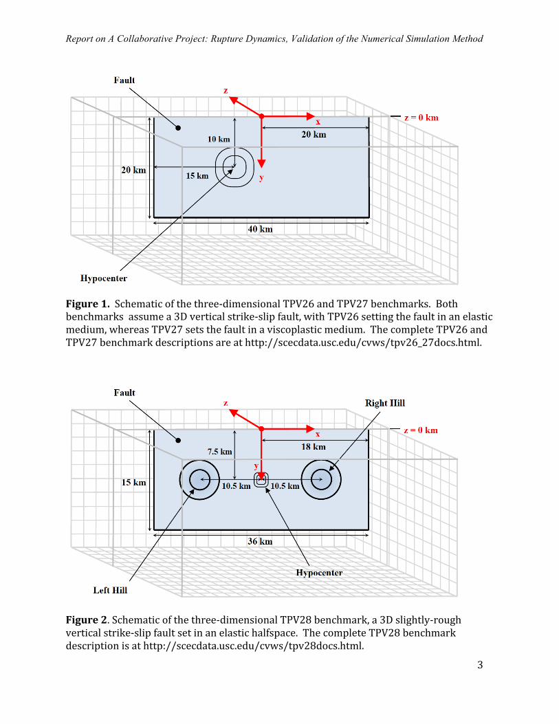
In late 2013 to early 2014, our group designed then tackled the 3D elastic and viscoplastic planar vertical strike-slip fault benchmarks, The Problem Versions 26 and 27 (Figure 1), and the case of a slightly-rough single vertical strike-slip fault set in an elastic medium, The Problem Version 28 (Figure 2). All three benchmarks, TPV26, TPV27, and TPV28, assume slip-weakening friction. Please see the Benchmark Descriptions page of our website, http://scecdata.usc.edu/cvws for more details about these (and our other) benchmarks, and our papers (Harris et al., SRL, 2009 and Harris et al., SRL, 2011) for more general information about our group's science goals.

The TPV26 and TPV27 (Figure 1) 2013-2014 benchmarks examine what happens if one implements elastic versus viscoplastic assumptions for the response of the rocks surrounding a vertical strike-slip fault. This case has an indirect application to source and ground motion simulations of large strike-slip earthquakes in southern California and elsewhere. As shown by co-PI Michael Barall in his March 14, 2014 SCEC workshop presentation (http://scecdata.usc.edu/cvws/download/mar14_2014/Barall_TPV26_TPV27_Results_v07.pdf), some viscoplastic parameter choices may lead to big changes in earthquake source behavior, including a spontaneously propagating rupture not even making it all of the way up to the earth’s surface, whereas the companion case of the same source set in an elastic medium produces surface rupture (Figure 3a).


3

Figure 1. Schematic of the three-‐dimensional TPV26 and TPV27 benchmarks. Both benchmarks assume a 3D vertical strike-‐slip fault, with TPV26 setting the fault in an elastic medium, whereas TPV27 sets the fault in a viscoplastic medium. The complete TPV26 and TPV27 benchmark descriptions are at http://scecdata.usc.edu/cvws/tpv26_27docs.html.

Figure 2. Schematic of the three-‐dimensional TPV28 benchmark, a 3D slightly-‐rough vertical strike-‐slip fault set in an elastic halfspace. The complete TPV28 benchmark description is at http://scecdata.usc.edu/cvws/tpv28docs.html.


4

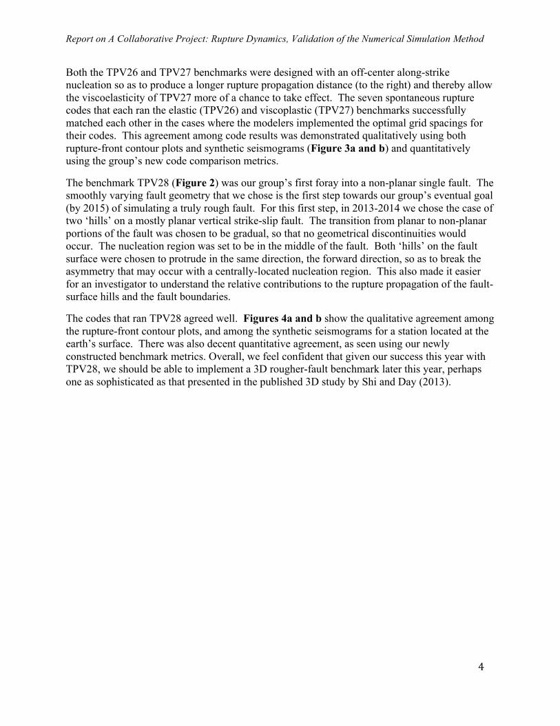
Both the TPV26 and TPV27 benchmarks were designed with an off-center along-strike nucleation so as to produce a longer rupture propagation distance (to the right) and thereby allow the viscoelasticity of TPV27 more of a chance to take effect. The seven spontaneous rupture codes that each ran the elastic (TPV26) and viscoplastic (TPV27) benchmarks successfully matched each other in the cases where the modelers implemented the optimal grid spacings for their codes. This agreement among code results was demonstrated qualitatively using both rupture-front contour plots and synthetic seismograms (Figure 3a and b) and quantitatively using the group’s new code comparison metrics.

The benchmark TPV28 (Figure 2) was our group’s first foray into a non-planar single fault. The smoothly varying fault geometry that we chose is the first step towards our group’s eventual goal (by 2015) of simulating a truly rough fault. For this first step, in 2013-2014 we chose the case of two ‘hills’ on a mostly planar vertical strike-slip fault. The transition from planar to non-planar portions of the fault was chosen to be gradual, so that no geometrical discontinuities would occur. The nucleation region was set to be in the middle of the fault. Both ‘hills’ on the fault surface were chosen to protrude in the same direction, the forward direction, so as to break the asymmetry that may occur with a centrally-located nucleation region. This also made it easier for an investigator to understand the relative contributions to the rupture propagation of the fault-surface hills and the fault boundaries.

The codes that ran TPV28 agreed well. Figures 4a and b show the qualitative agreement among the rupture-front contour plots, and among the synthetic seismograms for a station located at the earth’s surface. There was also decent quantitative agreement, as seen using our newly constructed benchmark metrics. Overall, we feel confident that given our success this year with TPV28, we should be able to implement a 3D rougher-fault benchmark later this year, perhaps one as sophisticated as that presented in the published 3D study by Shi and Day (2013).


5

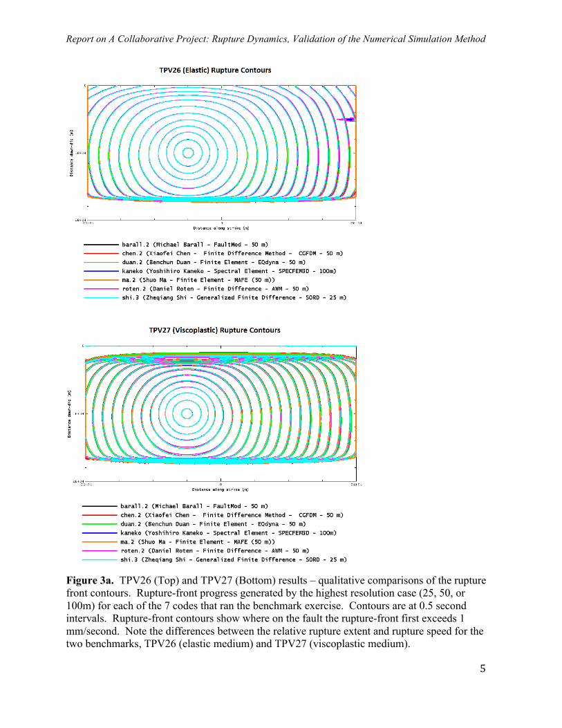
Figure 3a. TPV26 (Top) and TPV27 (Bottom) results – qualitative comparisons of the rupture front contours. Rupture-front progress generated by the highest resolution case (25, 50, or 100m) for each of the 7 codes that ran the benchmark exercise. Contours are at 0.5 second intervals. Rupture-front contours show where on the fault the rupture-front first exceeds 1 mm/second. Note the differences between the relative rupture extent and rupture speed for the two benchmarks, TPV26 (elastic medium) and TPV27 (viscoplastic medium).


6

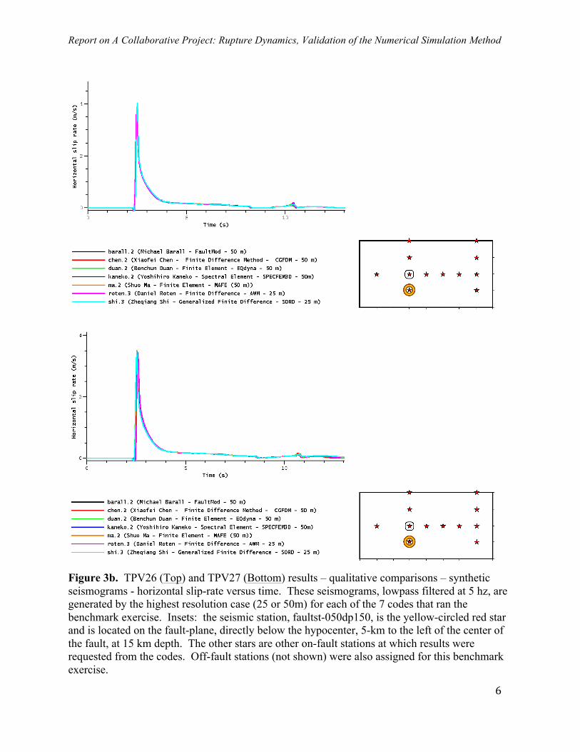
Figure 3b. TPV26 (Top) and TPV27 (Bottom) results – qualitative comparisons – synthetic seismograms - horizontal slip-rate versus time. These seismograms, lowpass filtered at 5 hz, are generated by the highest resolution case (25 or 50m) for each of the 7 codes that ran the benchmark exercise. Insets: the seismic station, faultst-050dp150, is the yellow-circled red star and is located on the fault-plane, directly below the hypocenter, 5-km to the left of the center of the fault, at 15 km depth. The other stars are other on-fault stations at which results were requested from the codes. Off-fault stations (not shown) were also assigned for this benchmark exercise.


7

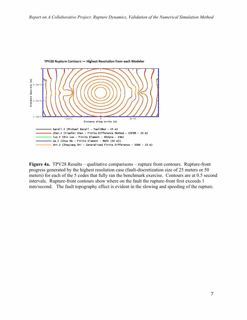
Figure 4a. TPV28 Results – qualitative comparisons – rupture front contours. Rupture-front progress generated by the highest resolution case (fault-discretization size of 25 meters or 50 meters) for each of the 5 codes that fully ran the benchmark exercise. Contours are at 0.5 second intervals. Rupture-front contours show where on the fault the rupture-front first exceeds 1 mm/second. The fault topography effect is evident in the slowing and speeding of the rupture.


8

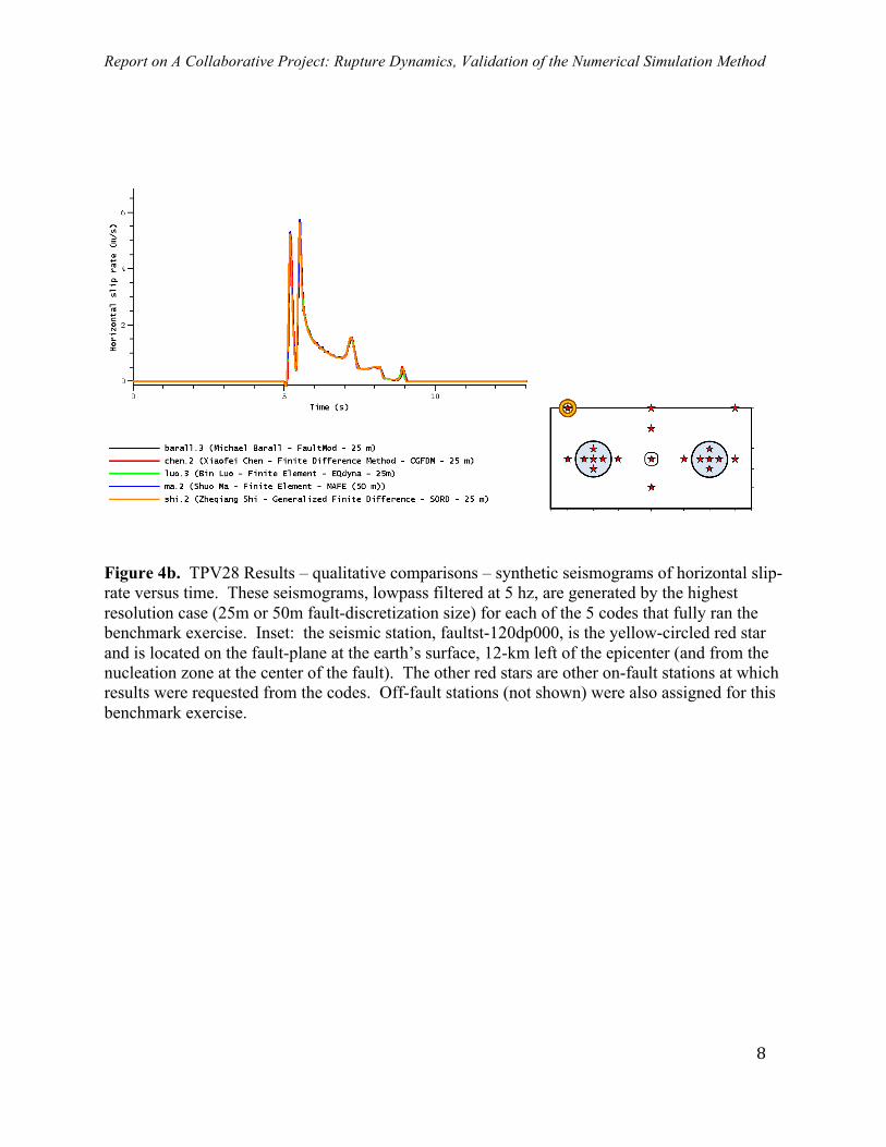
Figure 4b. TPV28 Results – qualitative comparisons – synthetic seismograms of horizontal slip-rate versus time. These seismograms, lowpass filtered at 5 hz, are generated by the highest resolution case (25m or 50m fault-discretization size) for each of the 5 codes that fully ran the benchmark exercise. Inset: the seismic station, faultst-120dp000, is the yellow-circled red star and is located on the fault-plane at the earth’s surface, 12-km left of the epicenter (and from the nucleation zone at the center of the fault). The other red stars are other on-fault stations at which results were requested from the codes. Off-fault stations (not shown) were also assigned for this benchmark exercise.


9

2013-2014 RESULTS – QUANTITATIVE METRICS

An exciting new development this year is quantitative metrics. Although we had discussed the creation and implementation of quantitative metrics during previous years, and a few ideas had been presented at a previous year’s workshop, we were still only qualitatively comparing our spontaneous rupture earthquake simulation results because we did not yet have a rigorous quantitative metric to apply to our vast collection of modeling ‘data’. While qualitative comparisons have their benefits – the human eye is gifted at discerning differences – we have long been curious about how the comparisons would fare quantitatively.

This year we have now advanced from this operative-mode of qualitative-only comparisons, to our quantitative-comparisons goal, with some finishing touches likely occurring for future metrics implementation. This accomplishment of the development and implementation of quantitative metrics is based on the hard work and vision of co-PI Michael Barall. Michael Barall presented his new metrics work at our March 14, 2014 SCEC workshop, and welcomed group discussion about all aspects of it. His new approach, which received voices of approval at the workshop, is available for viewing at http://scecdata.usc.edu/cvws/download/mar14_2014/Barall_metrics_v05.pdf. Community comments are also welcome.

Challenges for our project’s comparison metrics include the vast quantity of spontaneous rupture code modeling results that we have generated as of early-March 2014 (8.6 GB), the impressive number of benchmarks that we have performed to date (39), the number of participating modelers and codes (36), the number of modeler-uploaded files (100,000), and the number of requested results per benchmark (14 on average). This has led to more than 560,000 pairs of modeling results to compare. In the next two sections we discuss and present our new quantitative metrics for time-series modeling ‘data’ and for rupture-front contour plots, the latter of which tracks the progress of the simulated earthquake on the fault surface(s).

TIME-SERIES QUANTITATIVE METRICS

The spontaneous-rupture modeling results from our code comparison exercise are numerous in both type and quantity. For each of the benchmark exercises conducted by each of the participating codes, on-fault time series for slip, slip-rate, shear stress, and normal stress, all as a function of time, have been computed by each code at a set of pre-assigned on-fault seismic stations. Each code has also provided, for each benchmark, and for each pre-assigned off-fault seismic station, the computed results of displacement and velocity as a function of time. Each benchmark exercise has had on average 10 on-fault and 8 off-fault stations, leading to a considerable collection of synthetic time-series data. Figures 3b and 4b, which depict horizontal slip-rate versus time for just one of the on-fault stations in each of the three benchmarks TPV26, TPV27, and TPV28, are showing just a miniscule subset of the total amount of time-series information collected from our spontaneous rupture simulation codes for all of the benchmark exercises.

After the modelers use their codes to provide time-series results for each on-fault and off-fault station in a benchmark exercise, there still needs to be some post-processing to make these results useable for a quantitative comparison. These processing steps include a uniform filtering of the data, e.g., a low-pass 5-hz filter is applied to slip-rate, shear stress, normal stress, and


10

velocity modeling results. It is also reasonable that the time-series information generated by the codes for different spatial directions at each seismic station be combined into vector-valued time-series. For each on-fault station’s time-series results, this is achieved by combining the two-directional components of data to produce 2D slip, 2D slip-rate, and 2D shear-stress time-series. For each off-fault station’s time-series results this is achieved by combining each directional component to produce 3D displacement and 3D velocity time-series. Time-series metrics also allow for quantifications of time-differences, the time-shift that may enable two sets of time-series to match each other better.

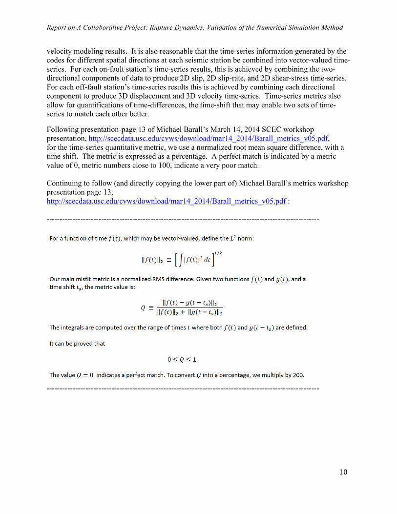
Following presentation-page 13 of Michael Barall’s March 14, 2014 SCEC workshop presentation, http://scecdata.usc.edu/cvws/download/mar14_2014/Barall_metrics_v05.pdf, for the time-series quantitative metric, we use a normalized root mean square difference, with a time shift. The metric is expressed as a percentage. A perfect match is indicated by a metric value of 0, metric numbers close to 100, indicate a very poor match. Continuing to follow (and directly copying the lower part of) Michael Barall’s metrics workshop presentation page 13, http://scecdata.usc.edu/cvws/download/mar14_2014/Barall_metrics_v05.pdf : ---------------------------------------------------------------------------------------------------------

---------------------------------------------------------------------------------------------------------


11

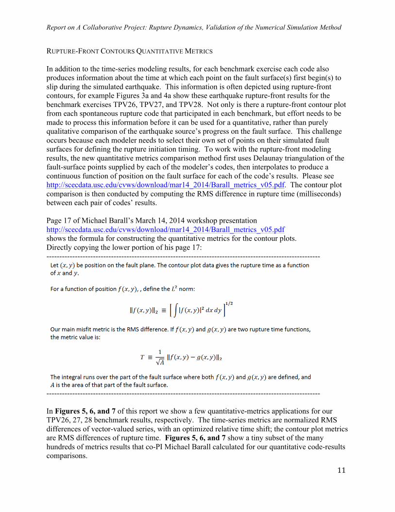
RUPTURE-FRONT CONTOURS QUANTITATIVE METRICS In addition to the time-series modeling results, for each benchmark exercise each code also produces information about the time at which each point on the fault surface(s) first begin(s) to slip during the simulated earthquake. This information is often depicted using rupture-front contours, for example Figures 3a and 4a show these earthquake rupture-front results for the benchmark exercises TPV26, TPV27, and TPV28. Not only is there a rupture-front contour plot from each spontaneous rupture code that participated in each benchmark, but effort needs to be made to process this information before it can be used for a quantitative, rather than purely qualitative comparison of the earthquake source’s progress on the fault surface. This challenge occurs because each modeler needs to select their own set of points on their simulated fault surfaces for defining the rupture initiation timing. To work with the rupture-front modeling results, the new quantitative metrics comparison method first uses Delaunay triangulation of the fault-surface points supplied by each of the modeler’s codes, then interpolates to produce a continuous function of position on the fault surface for each of the code’s results. Please see http://scecdata.usc.edu/cvws/download/mar14_2014/Barall_metrics_v05.pdf. The contour plot comparison is then conducted by computing the RMS difference in rupture time (milliseconds) between each pair of codes’ results. Page 17 of Michael Barall’s March 14, 2014 workshop presentation http://scecdata.usc.edu/cvws/download/mar14_2014/Barall_metrics_v05.pdf shows the formula for constructing the quantitative metrics for the contour plots. Directly copying the lower portion of his page 17: ----------------------------------------------------------------------------------------------------------

---------------------------------------------------------------------------------------------------------- In Figures 5, 6, and 7 of this report we show a few quantitative-metrics applications for our TPV26, 27, 28 benchmark results, respectively. The time-series metrics are normalized RMS differences of vector-valued series, with an optimized relative time shift; the contour plot metrics are RMS differences of rupture time. Figures 5, 6, and 7 show a tiny subset of the many hundreds of metrics results that co-PI Michael Barall calculated for our quantitative code-results comparisons.


12

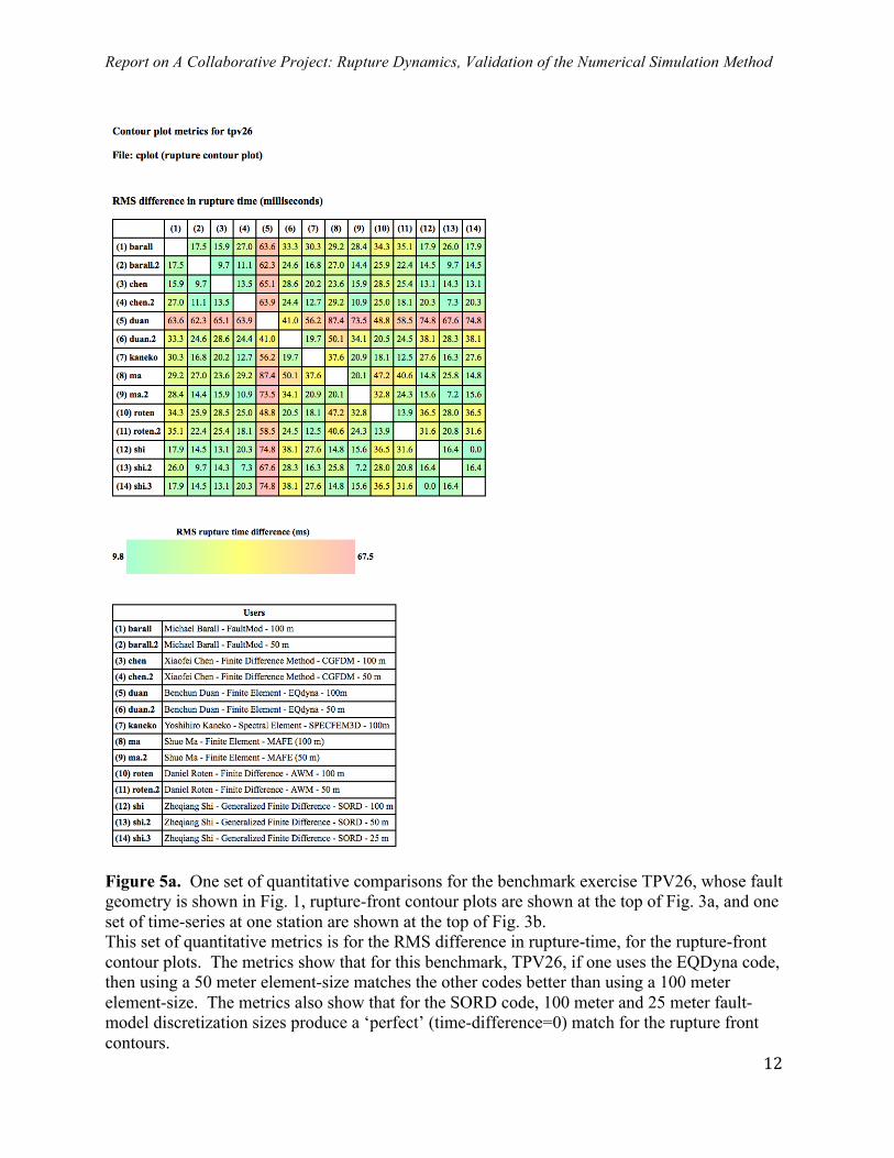
Figure 5a. One set of quantitative comparisons for the benchmark exercise TPV26, whose fault geometry is shown in Fig. 1, rupture-front contour plots are shown at the top of Fig. 3a, and one set of time-series at one station are shown at the top of Fig. 3b. This set of quantitative metrics is for the RMS difference in rupture-time, for the rupture-front contour plots. The metrics show that for this benchmark, TPV26, if one uses the EQDyna code, then using a 50 meter element-size matches the other codes better than using a 100 meter element-size. The metrics also show that for the SORD code, 100 meter and 25 meter fault-model discretization sizes produce a ‘perfect’ (time-difference=0) match for the rupture front contours.


13

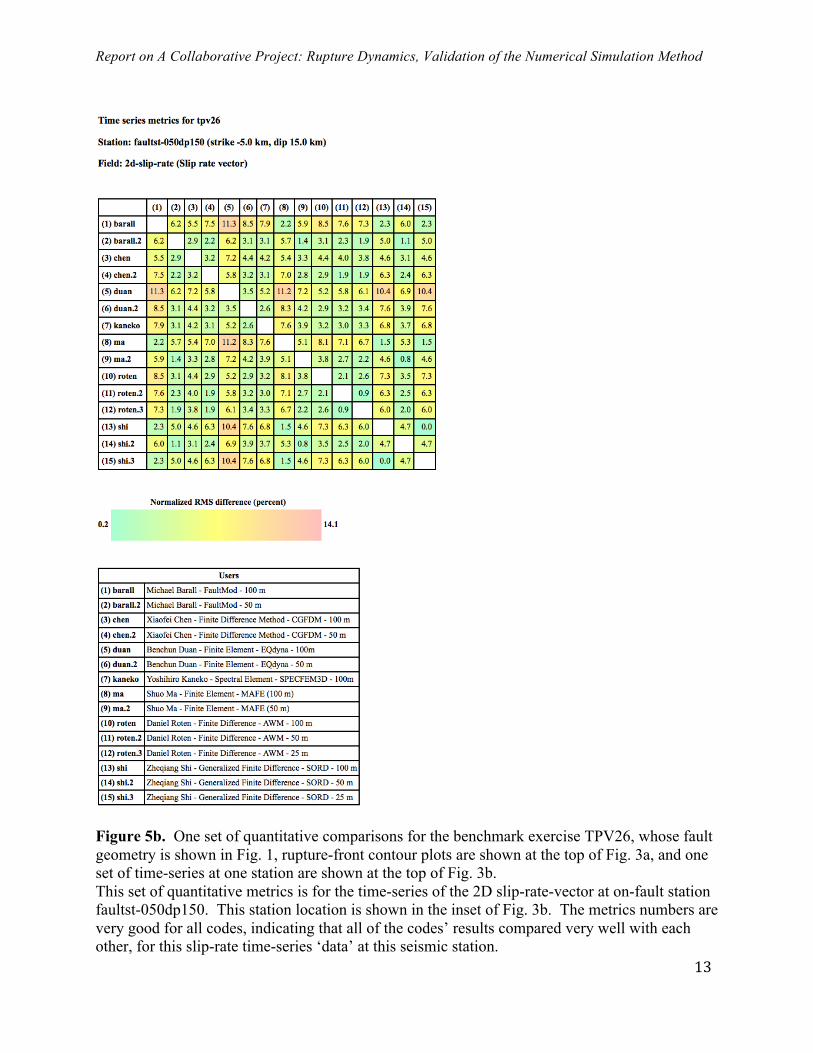
Figure 5b. One set of quantitative comparisons for the benchmark exercise TPV26, whose fault geometry is shown in Fig. 1, rupture-front contour plots are shown at the top of Fig. 3a, and one set of time-series at one station are shown at the top of Fig. 3b. This set of quantitative metrics is for the time-series of the 2D slip-rate-vector at on-fault station faultst-050dp150. This station location is shown in the inset of Fig. 3b. The metrics numbers are very good for all codes, indicating that all of the codes’ results compared very well with each other, for this slip-rate time-series ‘data’ at this seismic station.


14

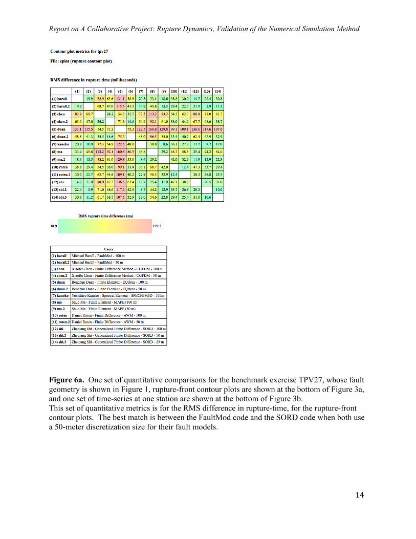
Figure 6a. One set of quantitative comparisons for the benchmark exercise TPV27, whose fault geometry is shown in Figure 1, rupture-front contour plots are shown at the bottom of Figure 3a, and one set of time-series at one station are shown at the bottom of Figure 3b. This set of quantitative metrics is for the RMS difference in rupture-time, for the rupture-front contour plots. The best match is between the FaultMod code and the SORD code when both use a 50-meter discretization size for their fault models.


15

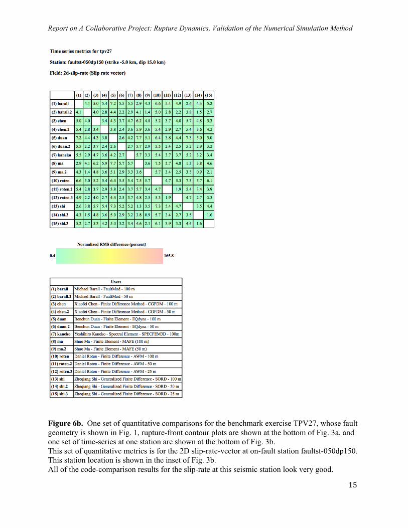
Figure 6b. One set of quantitative comparisons for the benchmark exercise TPV27, whose fault geometry is shown in Fig. 1, rupture-front contour plots are shown at the bottom of Fig. 3a, and one set of time-series at one station are shown at the bottom of Fig. 3b. This set of quantitative metrics is for the 2D slip-rate-vector at on-fault station faultst-050dp150. This station location is shown in the inset of Fig. 3b. All of the code-comparison results for the slip-rate at this seismic station look very good.


16

Figure 7a. One set of quantitative comparisons for the benchmark exercise TPV28, whose fault geometry is shown in Fig. 2, rupture-front contour plots are shown in Fig. 4a, and one set of time-series at one station are shown in Fig. 4b. This set of quantitative metrics is for the RMS difference in rupture-time, for the rupture-front contour plots. In this set of metrics, it appears that the FaultMod code matches the timing of most of the other codes better when using a 50-meter rather than a 100-meter element size for the fault model.


17

Figure 7b. One set of quantitative comparisons for the benchmark exercise TPV28, whose fault geometry is shown in Fig. 2, rupture-front contour plots are shown in Fig. 4a, and one set of time-series at one station are shown in Fig. 4b. This station location is shown in the inset of Fig. 4b. These quantitative metrics are for the 2D slip-rate-vector at on-fault station faultst-120dp000. The best matches are between the MAFE and SORD codes when both use a 50-meter discretization size for their fault models.


18

FUTURE PLANS: In mid- to late-2014, using 2014 funds, we have proposed (in our hopefully-funded SCEC 2014 proposal) to continue our investigations of non-planar fault geometry, and to also separately consider the case of a 1D material-velocity structure. Both of these topics, non-planarity, and inhomogeneous velocity structure are issues of high-interest in the earthquake science and ground motion applications communities.

FUNDING:

These benchmark exercises were funded through the SCEC 2013 research proposal review process. Some of the SCEC funding for this project is from a gift by PG&E to SCEC/USC.

REFERENCES:

Harris, R.A., Numerical simulations of large earthquakes: dynamic rupture propagation on heterogeneous faults, Pure and Applied Geophysics, vol. 161, no. 11/12, pp. 2171-2181, DOI: 10.1007/s00024-004-2556-8, 2004.

Harris, R.A., M. Barall, R. Archuleta, E. Dunham, B. Aagaard, J.P. Ampuero, H. Bhat, V. Cruz-Atienza, L. Dalguer, P. Dawson, S. Day, B. Duan, G. Ely, Y. Kaneko, Y. Kase, N. Lapusta, Y. Liu, S. Ma, D. Oglesby, K. Olsen, A. Pitarka, S. Song, E. Templeton, The SCEC/USGS Dynamic Earthquake Rupture Code Verification Exercise, Seism. Res. Lett., vol. 80, no. 1, p. 119-126, doi: 10.1785/gssrl.80.1.119, 2009.

Harris, R.A., M. Barall, D.J. Andrews, B. Duan, E.M. Dunham, S. Ma, A.-A. Gabriel, Y. Kaneko, Y. Kase, B. Aagaard, D. Oglesby, J.-P. Ampuero, T.C. Hanks, N. Abrahamson, Verifying a computational method for predicting extreme ground motion, Seism. Res. Lett., vol. 82, no. 5, p. 638-644, doi: 10.1785/gssrl.82.5.638, 2011.

Shi, Z., and S.M. Day, Rupture dynamics and ground motion from 3-D rough-fault simulations, J. Geophys. Res., vol. 118, 1122-1141, doi: doi:10.1002/jgrb.50094, 2013.


19

Thank you to our 2013-2014

GOLD-STAR DYNAMIC RUPTURE MODELERS

(who simulated one or more of the 2013-2014 benchmark exercises)

Michael Barall

Xiaofei Chen

Ben Duan

Alice Gabriel

Yoshi Kaneko

Bin Luo

Shuo Ma

Daniel Roten

Zheqiang Shi

Zhenguo Zhang

Date post:	21-Mar-2022
Category:	Documents
Upload:	others
View:	3 times
Download:	0 times

Final Report Submitted by Ruth Harris to SCEC March 20, 2014

Documents