S65

Bulletin of the Seismological Society of America, 90, 6B, pp. S65–S76, December 2000

The SCEC Southern California Reference Three-Dimensional Seismic

Velocity Model Version 2

by Harold Magistrale, Steven Day, Robert W. Clayton, and Robert Graves

Abstract We describe Version 2 of the three-dimensional (3D) seismic velocitymodel of southern California developed by the Southern California Earthquake Cen-ter and designed to serve as a reference model for multidisciplinary research activitiesin the area. The model consists of detailed, rule-based representations of the majorsouthern California basins (Los Angeles basin, Ventura basin, San Gabriel Valley,San Fernando Valley, Chino basin, San Bernardino Valley, and the Salton Trough),embedded in a 3D crust over a variable depth Moho. Outside of the basins, the modelcrust is based on regional tomographic results. The model Moho is represented by asurface with the depths determined by the receiver function technique. Shallow basinsediment velocities are constrained by geotechnical data. The model is implementedin a computer code that generates any specified 3D mesh of seismic velocity anddensity values. This parameterization is convenient to store, transfer, and update asnew information and verification results become available.

Introduction

The dense population and active tectonics of southernCalifornia necessitate extensive seismic hazard evaluationsthat include precise earthquake location determinations, pathand site effect studies, and strong ground motion simula-tions. These studies require a realistic three-dimensional(3D) seismic velocity model defined on spatial scales appro-priate for each application. Here we describe a 3D seismicvelocity model for southern California assembled from geo-logical and geophysical data and designed to serve as a ref-erence model for multidisciplinary research activities in thearea.

A velocity model, to be widely useful, must integratedata from multiple disciplines, including seismic imaging,geologic mapping, and geotechnical investigations, in orderto capture the wide range of spatial scales that are importantfor both basic research and earthquake hazard applications.Consider, for example, the problem of deterministic 3Dmodeling of long period (�1 sec) strong ground motion insouthern California. Regional seismic tomography provides3D seismic velocity information with resolution on the orderof tens of kilometers (Magistrale et al., 1992; Zhou, 1994;Hauksson, 2000). This resolution is useful for modeling thepropagation of long-period seismic waves in crystallinebasement rocks outside of the sedimentary basins, wherewavelengths are long and velocity variations are relativelysmall. In the basins, however, much higher spatial resolutionis required: basin depths are typically less than 10 km, andseismic velocities vary dramatically. In the low-velocity ba-sin sediments, 1-sec S waves have wavelengths ranging from

a few kilometers in the deep basins, down to only a fewhundred meters in the shallow basin layers. Also, importantamplification and interference effects are likely to be local-ized near the basin edges, which therefore need to be wellresolved. Geologic mapping, geotechnical investigations,and borehole velocity logs can provide the necessary highspatial resolution.

The Southern California Earthquake Center (SCEC) hassupported an effort to develop a standard 3D referencemodel for southern California. The designation “referencemodel” is meant to emphasize the following characteristics.(1) The model incorporates contributions from multipletypes of data. (2) It represents a standard agreed to amonga large number of researchers working in southern Califor-nia, against which anomalies (in, e.g., seismic travel times,waveforms, and amplitudes; gravity; and borehole data) canbe identified, quantified, and compared. (3) The model de-scription is reviewed and maintained by SCEC and madewidely available, and its periodic revisions are documentedand tracked by version number. (4) By integrating a large,diverse body of both seismic and nonseismic data, the ref-erence model provides a starting model for application ofperturbative approaches to the 3D inversion of seismic traveltime and waveform data. A prototype reference model (Mag-istrale et al., 1996; we will refer to it as Version 0) has beenwidely used for simulating ground motions from past earth-quakes (e.g., Wald and Graves, 1998) as well as for esti-mating basin effects from potential future earthquakes (e.g.,Olsen et al., 1996). The need for a single standard reference

S66 H. Magistrale, S. Day, R. W. Clayton and R. Graves

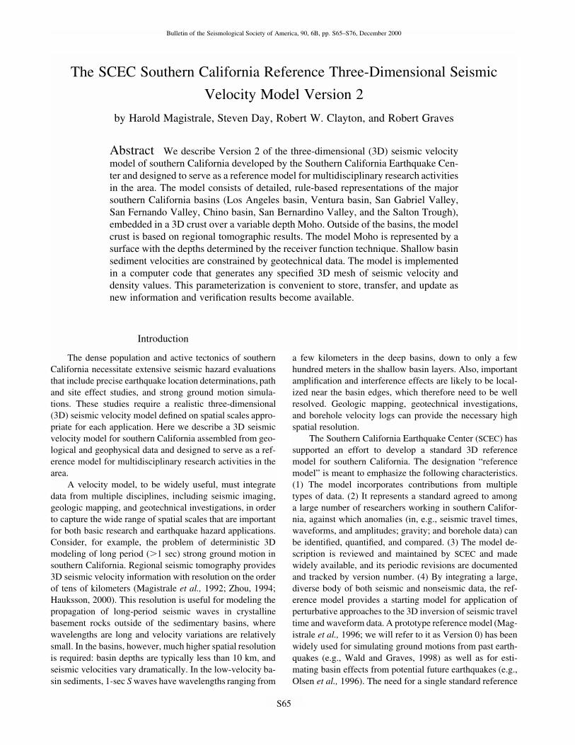
Figure 1. Location map of southern California showing the extent of the basin mod-els (heavy black lines) and basin names. Light black lines are faults. Inset shows lo-cation of figure area; western North America is shaded.

model motivated the much more comprehensive model de-velopment reported here.

Version 2 of the SCEC reference model consists of de-tailed, rule-based representations of the major southern Cali-fornia basins (Fig. 1) embedded in a 3D crust over a variabledepth Moho. The model includes the populated Los Angelesarea basins (Los Angeles basin, Ventura basin, San GabrielValley, San Fernando Valley, Chino basin, and San Bernar-dino Valley), and the Salton Trough. The basins are param-eterized as a set of objects (constructed from geological, geo-physical, and geotechnical data) and rules implemented in acomputer code that generates any specified 3D mesh of seis-mic velocity and density values. This parameterization isconvenient to store, transfer, and update as new informationand verification results become available. It allows any dis-tribution of velocities; for example, fast-over-slow velocitiesare easily modeled. A fine spatial resolution is achieved bythe use of geologic information to constrain the locationsand ages of structural and stratigraphic boundaries. Outsideof the basins, the model crust is based on regional tomo-graphic results. The model Moho is represented by a surfacewith the depths determined by the receiver function tech-nique.

Several studies in this special volume (Field, 2000; Leeand Anderson, 2000; Olsen, 2000; Steidl, 2000) use Version1 of the SCEC reference model (Magistrale et al., 1998).Version 1 contains the Los Angeles area basins in a 1D crustover a constant depth Moho. The Version 1 model improvedthe Version 0 model of Magistrale et al. (1996) by addingthe Ventura basin, Chino basin, and San Bernardino Valley,and revising the San Fernando Valley. Version 2 is an ad-

vance over Version 1 in that it includes the Salton Trough,a 3D distribution of crustal velocities outside of the basins,a 3D Moho, and detailed shallow basin velocities from geo-technical logs. The ground-motion simulations reported inthis volume (Olsen, 2000) focused on the Los Angeles areabasins and imposed a VS lower bound of 1 km/sec (due tocomputational limitations), so the conclusions based onthose simulations would be little affected by the Version 2modifications. Basin depth effects on ground motion re-ported in this volume (Field, 2000; Lee and Anderson, 2000;Steidl, 2000) use the depth to the 2.5 km/sec VS isovelocitysurface to define basin depth. In the Los Angeles area basinsthat isovelocity surface is the same in the Version 1 andVersion 2 models.

Model Construction

Reference Surfaces and Rule Definition

In the model sedimentary basins, VP is determined bythe application of empirical rules to interpolate propertiesfrom the model objects, and density and VS are derived fromVP. Outside and below the basins, VP and VS are assignedby interpolation from the regional tomographic results ofHauksson (2000). Within the basins, VP and VS in the top300 m are constrained by geotechnical borehole seismic ve-locity data. Where VP and VS are independently specified,the density is derived from VP.

There exists a great deal of information about the ageand depth of the sediments in the Los Angeles area basinsfrom oil and water exploration activities and other geologic

The SCEC Southern California Reference Three-Dimensional Seismic Velocity Model Version 2 S67

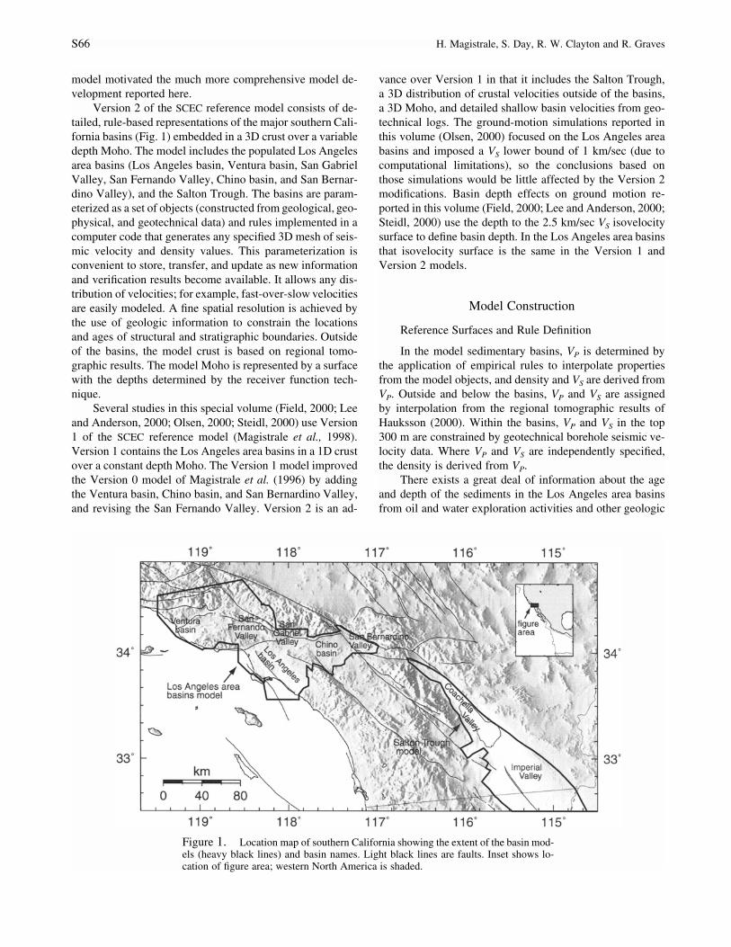
Figure 2. Sources of the information used to con-struct the basin model reference surfaces for the LosAngeles area (top panel) and Salton Trough (lowerpanel).

studies (Fig. 2). From this information, we define referencesurfaces (objects) of known depth and age in the detailedportion of the model representing the sedimentary basins.We examine structural cross sections and maps to definewidespread, well-defined reference surfaces representing stra-tigraphic horizons, sediment-basement contacts, and faults(many of the surfaces are in multiple pieces). The maps andcross sections are digitized, and the reference surfaces arecarefully interpolated and resampled on regular grids with aspacing of 100 to 300 meters. Uplift of each reference sur-face is estimated, or sometimes has been explicitly mapped(e.g., Wright, 1991).

Faust (1951) examined well surveys from North Amer-ica and determined an empirical relation between sedimentage, depth, and P-wave seismic velocity:

1/6V � k(da) (1)P

where VP is P-wave velocity, d is the maximum depth ofburial of the sediments, a is the sediment age, and k is aconstant. The one-sixth power reflects the tendency of sed-iments to compact as they are buried and to indurate as theyage (Dobrin, 1976). Age at any point in a basin can be in-terpolated from the reference surfaces. The constant k is cal-ibrated for each reference surface by comparison to oil wellsonic logs and seismic refraction surveys. At each point ofinterest within a basin (defined by a latitude, longitude, anddepth) for which the velocity is desired: (1) The age and kof the point are interpolated by comparing the point depthto the depths, ages, and k values of the reference surfaces atthe same latitude and longitude. (2) The maximum depth ofburial is found by correcting the current depth by any knownamount of uplift. (3) VP is determined from the Faust equa-tion. (4) Other physical parameters are derived: density isfound from VP using the relation of Nafe and Drake (1960);density is used to find Poisson’s ratio with the relation ofLudwig et al. (1970); VS is calculated from the P-wave ve-locity and Poisson’s ratio.

The seismic velocity structure of the Salton Trough hasbeen characterized by several seismic refraction studies(Fuis et al., 1982, 1984; Mooney and McMechan, 1982; Par-sons and McCarthy, 1996). Thus, instead of constructingreference surfaces from sediment stratigraphy information,the Salton Trough is modeled by digitizing VP cross sectionsderived from the seismic refraction lines (Fig. 2) and con-verting the cross sections into isovelocity surfaces. At a pointof interest, VP is interpolated from the isovelocity surfaces,and the other properties are derived from VP as in step 4mentioned previously.

Los Angeles Basin and San Gabriel Valley

Wright (1991), in an extensive summary, presents struc-ture-contour maps of two widespread sedimentary strati-graphic horizons: the base of the Repetto Formation, about4.5 Ma; and the base of the Mohnian Stage, about 14 Ma.Age control of the stratigraphic horizons is from microfossils

(e.g., Blake, 1991). Wright (1991) also presents a contourmap of the amount of uplift during the Pasadenan defor-mation (3.5 Ma to present); we use this information to cor-rect current sediment depths to depth of maximum burial.McCulloh (1960) and Yerkes et al. (1965) show a structure-contour map of the top of crystalline basement rocks inferredmainly from gravity data. The age we use for this horizonis not the rock age, but rather an early Miocene age (20 Ma)that just predates the development of major basement reliefand so dates the base of the sediment fill. The age and dis-tribution of material at the ground surface is indicated onCalifornia Division of Mines and Geology (CDMG) geologicmaps (Jennings, 1962; Rogers, 1965, 1967; Jennings andStrand, 1969).

The Santa Monica area within the Los Angeles basin isof particular interest to strong-motion modelers because ofthe unexpectedly high damage to the area from the North-ridge earthquake (e.g., Gao et al., 1997). Wright (1991)shows four detailed cross sections that we use to refine theMohnian, Repetto, and basement surfaces in that area.

We calibrate the model by adjusting the constant k inthe Faust relation (equation 1) to match seven oil well sonic

S68 H. Magistrale, S. Day, R. W. Clayton and R. Graves

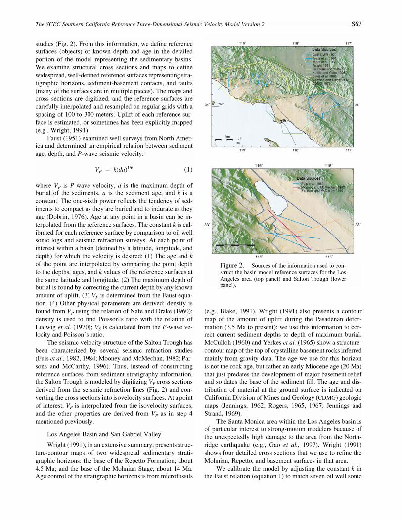
Figure 3. Oil well sonic logs (red) from Brocheret al. (1998) in the Los Angeles basin, San GabrielValley, and San Fernando Valley used to calibrate themodel (blue). Yellow triangles indicate oil well lo-cations.

logs (Fig. 3) in the Los Angeles basin and the San GabrielValley (Brocher et al., 1998). In the Los Angeles basin, k� 197; in the San Gabriel Valley, k � 218. The sonic logsindicate a VP inversion within the sediments of the San Ga-briel Valley. The inversion starts at a constant fraction (0.6)of the depth to the Mohnian reference surface and reaches aconstant �1250 m/sec about 400 m deeper. The inversionis modeled by subtracting the 1250 m/sec from the calcu-lated velocities, tapering the subtraction over the top 400 mof the inversion.

This version of the Los Angeles basin and the San Ga-briel Valley differs from Version 0 in the different values ofk calibrated from the oil well sonic logs, the San GabrielValley velocity inversion, and the Santa Monica area details.The current Los Angeles basin and San Gabriel Valley inVersion 2 are the same as in Version 1, except for the geo-technical constraints described subsequently.

San Fernando Valley and Ventura Basin

The San Fernando Valley and the Ventura basin sharesimilar stratigraphy and so are considered together. Yeats etal. (1988, 1994), Namson and Davis (1992), Huftile andYeats (1996), Davis et al. (1996), and Tsutsumi and Yeats(1999) present structural cross sections of the San FernandoValley and the Ventura basin from which we define a totalof 12 reference surfaces in 57 pieces. The lateral extent ofthe reference surfaces at the Earth’s surface is from a CDMGgeologic map (Jennings and Strand, 1969).

The 11 reference surfaces in the Ventura basin haveages of 0.5, 0.975, 1.5, 2.3, 5.0, 24, 37, 47, 67, 75, and 100Ma; lacking independent calibration, we set k � 180 for allthose surfaces to produce model velocities in the deepestsediments approaching the velocities of the surroundingbasement rock. In the San Fernando Valley, the seven ref-erences surfaces have ages of 2.0, 2.3, 5.0, 37, 67, 75, and100 Ma. Four oil well sonic logs (Fig. 3) are available in theSan Fernando Valley (Brocher et al., 1998); from these wedetermine a different k for each reference surface (k � 189,189, 160, 180, 123, 180, 180, respectively). We correct cur-rent sediment depth to maximum depth of burial by calcu-lating the average depth of each reference surface and, be-cause the strata are deformed largely by relatively recent (�1Ma, e.g., Huftile and Yeats, 1995) activity, assume any depthabove the average depth was formerly at least as deep as theaverage. If the current depth is below the average depth, thecurrent depth is used as the maximum depth of burial.

This version of the San Fernando Valley supplants theVersion 0 model. It uses entirely new reference surfaces, andnew k values calibrated to oil well sonic logs in the valley.The Version 0 model did not include the Ventura basin. TheVersion 2 San Fernando Valley and Ventura basin are thesame as in Version 1, except for the geotechnical constraintsdescribed subsequently.

San Bernardino and Chino Basins

The Chino and San Bernardino basins are shallow (gen-erally � 1 km deep) basins filled mostly with terrestrial sed-

iments. We use structural cross sections and maps of thedepth to the base of water-bearing strata from Departmentof Water Resources (1970) and Fife et al. (1976) to definethree reference surfaces: a 14.5 Ma Mohnian and a 6.0 MaMiocene (both limited to the westernmost portion of theChino basin), and the base of the water bearing strata. Theage and distribution of material at the ground surface is fromCDMG geologic maps (Rogers, 1965; 1967).

Hadley and Combs (1974) obtained a seismic refractionprofile in San Bernardino basin. We note that the top of their2.9 km/sec VP layer corresponds to the base of the waterbearing strata, and we interpret the top of that 2.9 km/seclayer to correspond to the top of weathered crystalline base-ment rock. Below the 2.9 km/sec layer, Hadley and Combs(1974) defined a 5.3 km/sec layer that we interpret to rep-resent hard rock, and we define a hard rock reference surfaceat a constant depth below the weathered basement surfaceto mark the bottom of the basin. We compare model velocityprofiles to the seismic refraction profile and calibrate themodel by adjusting the nominal ages of the weathered andhard basement surfaces (while keeping k fixed at 180) tomatch the refraction results. The final ages are 6.0 and 16.5Ma, respectively.

Frankel (1993) combined the Hadley and Combs (1974)refraction profile and water well logs to develop a model ofthe San Bernardino basin to use in ground-motion simula-tions. That model used the base of water bearing strata inthe well logs and the top of the 5.3 km/sec refraction profilelayer to define the top of the basement, and thus is dominated

The SCEC Southern California Reference Three-Dimensional Seismic Velocity Model Version 2 S69

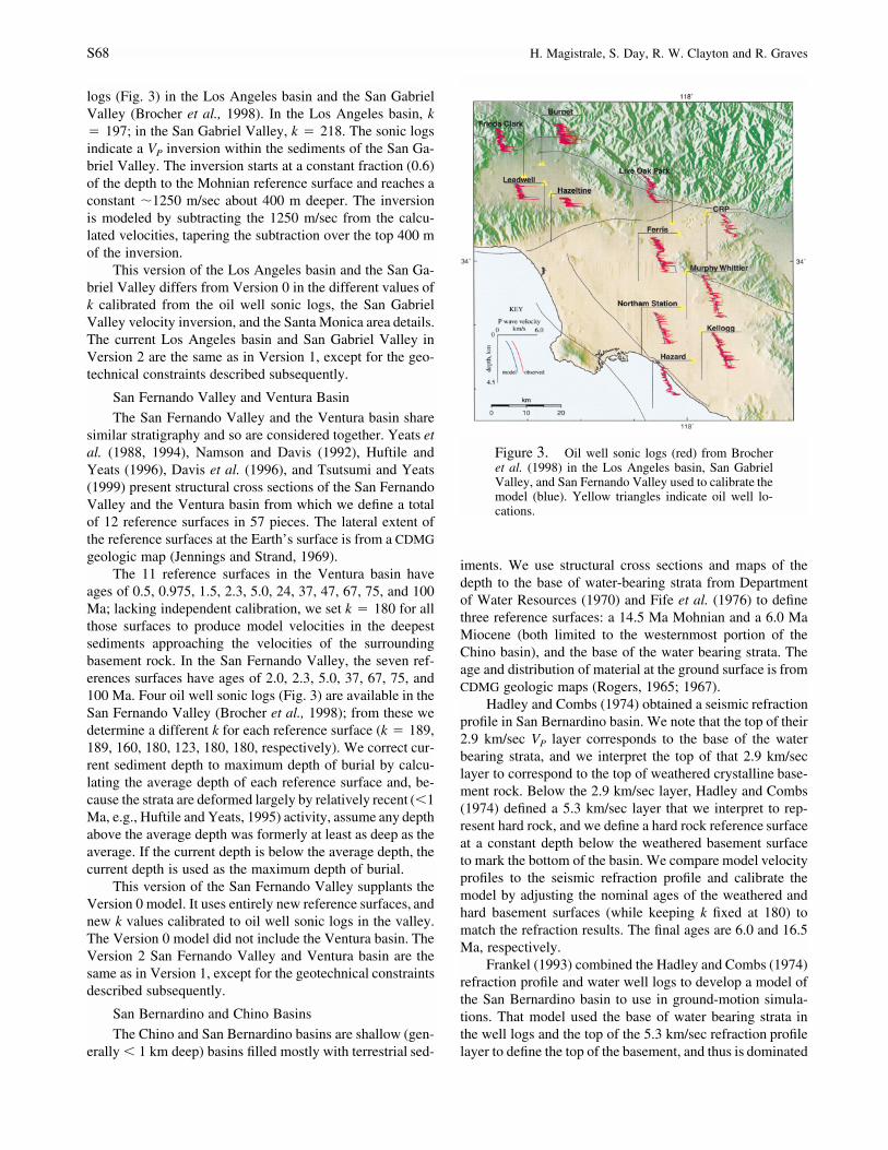
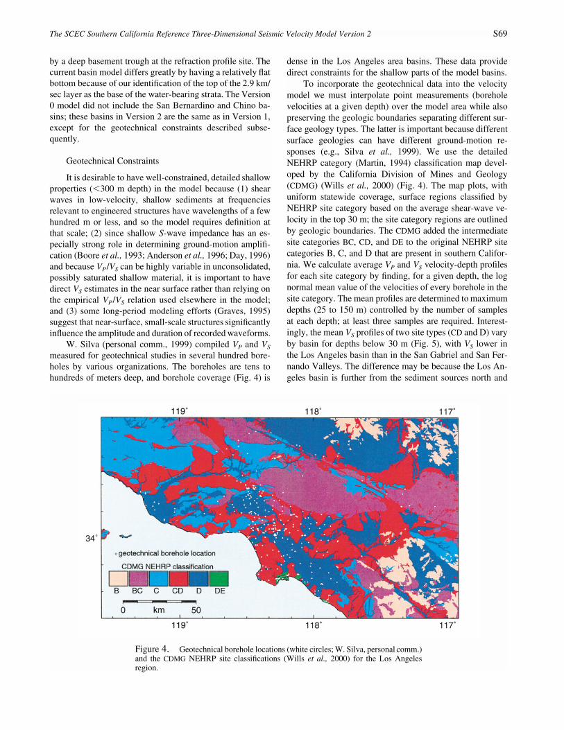
Figure 4. Geotechnical borehole locations (white circles; W. Silva, personal comm.)and the CDMG NEHRP site classifications (Wills et al., 2000) for the Los Angelesregion.

by a deep basement trough at the refraction profile site. Thecurrent basin model differs greatly by having a relatively flatbottom because of our identification of the top of the 2.9 km/sec layer as the base of the water-bearing strata. The Version0 model did not include the San Bernardino and Chino ba-sins; these basins in Version 2 are the same as in Version 1,except for the geotechnical constraints described subse-quently.

Geotechnical Constraints

It is desirable to have well-constrained, detailed shallowproperties (�300 m depth) in the model because (1) shearwaves in low-velocity, shallow sediments at frequenciesrelevant to engineered structures have wavelengths of a fewhundred m or less, and so the model requires definition atthat scale; (2) since shallow S-wave impedance has an es-pecially strong role in determining ground-motion amplifi-cation (Boore et al., 1993; Anderson et al., 1996; Day, 1996)and because VP/VS can be highly variable in unconsolidated,possibly saturated shallow material, it is important to havedirect VS estimates in the near surface rather than relying onthe empirical VP/VS relation used elsewhere in the model;and (3) some long-period modeling efforts (Graves, 1995)suggest that near-surface, small-scale structures significantlyinfluence the amplitude and duration of recorded waveforms.

W. Silva (personal comm., 1999) compiled VP and VS

measured for geotechnical studies in several hundred bore-holes by various organizations. The boreholes are tens tohundreds of meters deep, and borehole coverage (Fig. 4) is

dense in the Los Angeles area basins. These data providedirect constraints for the shallow parts of the model basins.

To incorporate the geotechnical data into the velocitymodel we must interpolate point measurements (boreholevelocities at a given depth) over the model area while alsopreserving the geologic boundaries separating different sur-face geology types. The latter is important because differentsurface geologies can have different ground-motion re-sponses (e.g., Silva et al., 1999). We use the detailedNEHRP category (Martin, 1994) classification map devel-oped by the California Division of Mines and Geology(CDMG) (Wills et al., 2000) (Fig. 4). The map plots, withuniform statewide coverage, surface regions classified byNEHRP site category based on the average shear-wave ve-locity in the top 30 m; the site category regions are outlinedby geologic boundaries. The CDMG added the intermediatesite categories BC, CD, and DE to the original NEHRP sitecategories B, C, and D that are present in southern Califor-nia. We calculate average VP and VS velocity-depth profilesfor each site category by finding, for a given depth, the lognormal mean value of the velocities of every borehole in thesite category. The mean profiles are determined to maximumdepths (25 to 150 m) controlled by the number of samplesat each depth; at least three samples are required. Interest-ingly, the mean VS profiles of two site types (CD and D) varyby basin for depths below 30 m (Fig. 5), with VS lower inthe Los Angeles basin than in the San Gabriel and San Fer-nando Valleys. The difference may be because the Los An-geles basin is further from the sediment sources north and

S70 H. Magistrale, S. Day, R. W. Clayton and R. Graves

Figure 5. Mean (unsmoothed log-normal) VS profiles (thick lines) of site categoriesCD and D for the Los Angeles basin (LAB, solid), San Fernando Valley (SFV, longdashes), and San Gabriel Valley (SGV, short dashes). Note differences below 30 mdepth. Thin lines are �1 r; the number of samples varies from 3 to 88 at differentdepths.

Figure 6. VP/VS for site categories C (shortdashes), CD (long dashes), D (solid), and DE (dots).Abbreviations as in Figure 5.

east of the basins than the two valleys, and so receives finergrained, seismically slower sediments. We use basin-specificmean profiles (defined by finding the mean velocities of theboreholes of each site type within each basin) for site typesCD and D.

Separate VP and VS mean profiles for all the site cate-gories are used; the VS profiles are smoothed by eye to re-move minor velocity inversions that result from the aver-aging process. VP/VS values derived from the (unsmoothed)mean profiles are about 1.7 to 2.5 in site category C, about1.7 to 3.5 in site categories CD and D (except for in the SanGabriel Valley, where category D VP/VS reaches about 5.5),and up to about 9.5 in category DE (Fig. 6). Site categoryBC had too few VP data to calculate VP/VS.

The velocity at a specific shallow point is found by (1)looking up the site category the point is in; (2) looking upnearby (�5 km distance) boreholes in the same site categorywith data at the same depth as the point; and (3) assigningthe velocity as a weighted combination of the appropriatemean profile and nearby boreholes. If there are no nearbyboreholes the velocity from that site type mean profile isused. This allows reasonable velocity values to be assignedto the areas where geotechnical data are sparse. If the pointis within 50 m of a borehole, the velocity from that boreholeis used, so the original borehole data can be recovered. Be-tween 50 m and 2 km (2 km and 5 km) the boreholes andgeneric profile are weighted by 2/3 and 1/3 (1/3 and 2/3),

The SCEC Southern California Reference Three-Dimensional Seismic Velocity Model Version 2 S71

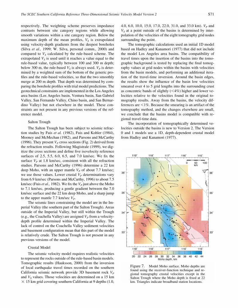
Figure 7. Model Moho surface. Moho depths arefound using the receiver-function technique and re-gional tomography crustal velocities except in theSalton Trough where the Moho depth is fixed at 22km. Triangles indicate broadband station locations.

respectively. The weighting scheme preserves impedancecontrasts between site category regions while allowingsmooth variations within a site category region. Below themaximum depth of the mean profiles, VS is extrapolatedusing velocity-depth gradients from the deepest boreholes(Silva et al., 1999; W. Silva, personal comm., 2000) andcompared to VS calculated by the rule-based scheme. Theextrapolated VS is used until it reaches a value equal to therule-based value, typically between 100 and 300 m depth;below 300 m, the rule-based VS is always used. VP is deter-mined by a weighted sum of the bottom of the generic pro-files and the rule-based velocities, so that the two smoothlymerge at 200 m depth. That depth was determined by com-paring the borehole profiles with trial model predictions. Thegeotechnical constraints are implemented in the Los Angelesarea basins (Los Angeles basin, Ventura basin, San GabrielValley, San Fernando Valley, Chino basin, and San Bernar-dino Valley) but not elsewhere in the model. These con-straints are not present in any previous versions of the ref-erence model.

Salton Trough

The Salton Trough has been subject to seismic refrac-tion studies by Fuis et al. (1982), Fuis and Kohler (1984),Mooney and McMechan (1982), and Parsons and McCarthy(1996). They present VP cross sections (Fig. 2) derived fromthe refraction results. Following Magistrale (1999), we dig-itize the cross sections and define five isovelocity referencesurfaces of 2.5, 5.5, 6.0, 6.5, and 7.0 km/sec. We fix thesurface VP at 1.8 km/sec, consistent with all the refractionstudies. Parsons and McCarthy (1996) determine a 22 kmdeep Moho, with an upper mantle VP of about 7.7 km/sec;we use those values. Lower crustal VP determinations varyfrom 6.9 km/sec (Parsons and McCarthy, 1996) to about 7.5km/sec (Fuis et al., 1982). We fix the VP just above the Mohoto 7.1 km/sec, producing a gentle gradient between the 7.0km/sec surface and the 22 km deep Moho, and a sharp jumpto the upper mantle 7.7 km/sec VP.

The seismic lines constraining the model are in the Im-perial Valley (the southern part of the Salton Trough). Areasoutside of the Imperial Valley, but still within the Trough(e.g., the Coachella Valley) are assigned VP from a velocity-depth profile determined within the Imperial Valley. Thelack of control on the Coachella Valley sediment velocitiesand basement configuration mean that this part of the modelis relatively crude. The Salton Trough is not present in anyprevious versions of the model.

Crustal Model

The seismic velocity model requires realistic velocitiesto represent the rocks outside of the rule-based basin models.Tomographic results (Hauksson, 2000) from the inversionof local earthquake travel times recorded on the southernCalifornia seismic network provide 3D basement rock VP

and VS values. Those velocities are determined on a 15 km� 15 km grid covering southern California at 9 depths (1.0,

4.0, 6.0, 10.0, 15.0, 17.0, 22.0, 31.0, and 33.0 km). VP andVS at a point outside of the basins is determined by inter-polation of the velocities of the eight tomography grid nodessurrounding the point.

The tomographic calculations used an initial 1D modelbased on Hadley and Kanamori (1977) that did not includethe model Los Angeles area basins. The compatibility oftravel times upon the insertion of the basins into the tomo-graphic background is tested by replacing the final tomog-raphy values at grid nodes within the basins with velocitiesfrom the basin models, and performing an additional itera-tion of the travel-time inversion. Around the basin edges,the results show the influence of the basin low velocitiessmeared over 4 to 5 grid lengths into the surrounding crustas concentric bands of slightly (�4%) higher and lower ve-locities relative to the velocities found in the original to-mography results. Away from the basins, the velocity dif-ferences are �1%. Because the smearing is an artifact of thetomography method, and the changes elsewhere are small,we conclude that the basins model is compatible with re-gional travel-time data.

The incorporation of tomographically determined ve-locities outside the basins is new to Version 2. The Version0 and 1 models use a 1D, depth-dependent crustal modelfrom Hadley and Kanamori (1977).

S72 H. Magistrale, S. Day, R. W. Clayton and R. Graves

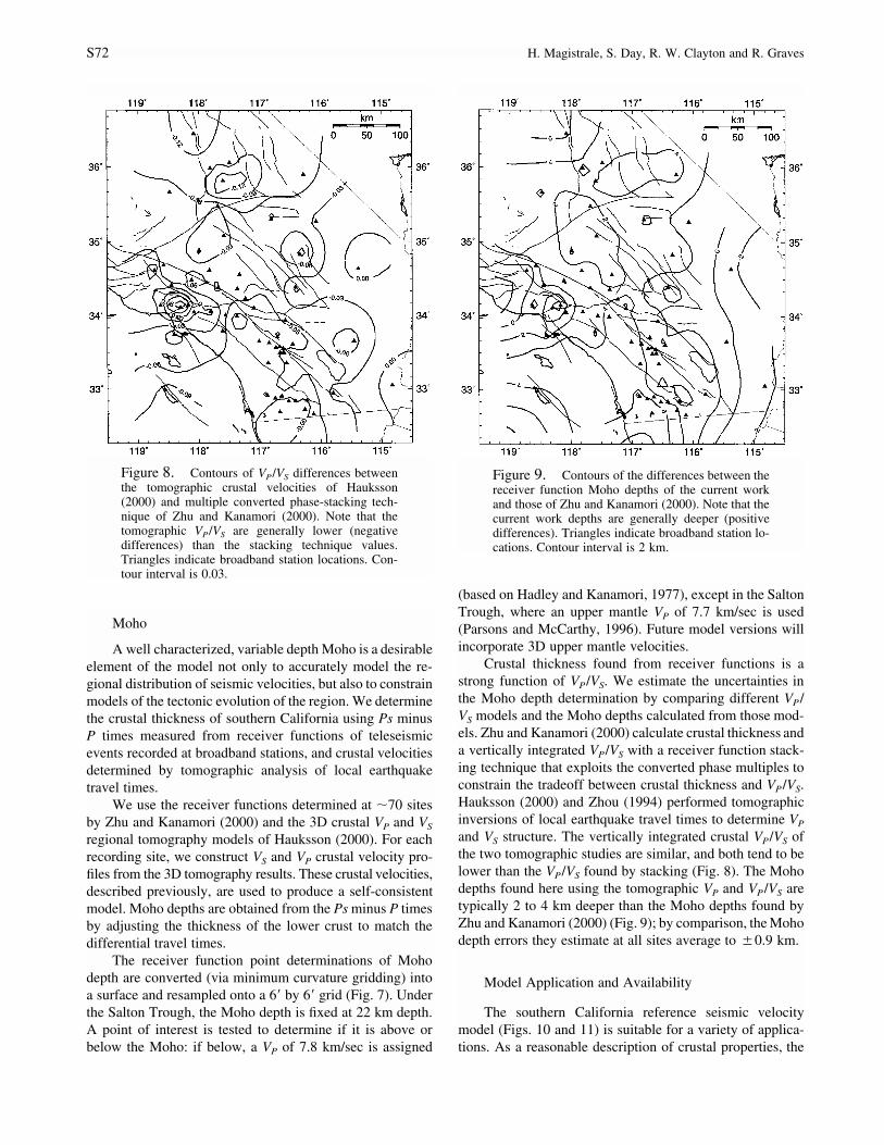
Figure 8. Contours of VP/VS differences betweenthe tomographic crustal velocities of Hauksson(2000) and multiple converted phase-stacking tech-nique of Zhu and Kanamori (2000). Note that thetomographic VP/VS are generally lower (negativedifferences) than the stacking technique values.Triangles indicate broadband station locations. Con-tour interval is 0.03.

Figure 9. Contours of the differences between thereceiver function Moho depths of the current workand those of Zhu and Kanamori (2000). Note that thecurrent work depths are generally deeper (positivedifferences). Triangles indicate broadband station lo-cations. Contour interval is 2 km.

Moho

A well characterized, variable depth Moho is a desirableelement of the model not only to accurately model the re-gional distribution of seismic velocities, but also to constrainmodels of the tectonic evolution of the region. We determinethe crustal thickness of southern California using Ps minusP times measured from receiver functions of teleseismicevents recorded at broadband stations, and crustal velocitiesdetermined by tomographic analysis of local earthquaketravel times.

We use the receiver functions determined at �70 sitesby Zhu and Kanamori (2000) and the 3D crustal VP and VS

regional tomography models of Hauksson (2000). For eachrecording site, we construct VS and VP crustal velocity pro-files from the 3D tomography results. These crustal velocities,described previously, are used to produce a self-consistentmodel. Moho depths are obtained from the Ps minus P timesby adjusting the thickness of the lower crust to match thedifferential travel times.

The receiver function point determinations of Mohodepth are converted (via minimum curvature gridding) intoa surface and resampled onto a 6� by 6� grid (Fig. 7). Underthe Salton Trough, the Moho depth is fixed at 22 km depth.A point of interest is tested to determine if it is above orbelow the Moho: if below, a VP of 7.8 km/sec is assigned

(based on Hadley and Kanamori, 1977), except in the SaltonTrough, where an upper mantle VP of 7.7 km/sec is used(Parsons and McCarthy, 1996). Future model versions willincorporate 3D upper mantle velocities.

Crustal thickness found from receiver functions is astrong function of VP/VS. We estimate the uncertainties inthe Moho depth determination by comparing different VP/VS models and the Moho depths calculated from those mod-els. Zhu and Kanamori (2000) calculate crustal thickness anda vertically integrated VP/VS with a receiver function stack-ing technique that exploits the converted phase multiples toconstrain the tradeoff between crustal thickness and VP/VS.Hauksson (2000) and Zhou (1994) performed tomographicinversions of local earthquake travel times to determine VP

and VS structure. The vertically integrated crustal VP/VS ofthe two tomographic studies are similar, and both tend to belower than the VP/VS found by stacking (Fig. 8). The Mohodepths found here using the tomographic VP and VP/VS aretypically 2 to 4 km deeper than the Moho depths found byZhu and Kanamori (2000) (Fig. 9); by comparison, the Mohodepth errors they estimate at all sites average to �0.9 km.

Model Application and Availability

The southern California reference seismic velocitymodel (Figs. 10 and 11) is suitable for a variety of applica-tions. As a reasonable description of crustal properties, the

The SCEC Southern California Reference Three-Dimensional Seismic Velocity Model Version 2 S73

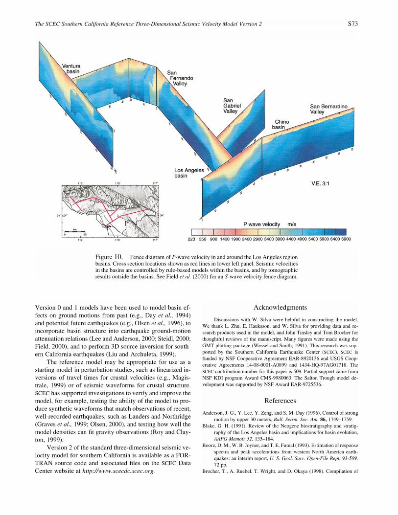
Figure 10. Fence diagram of P-wave velocity in and around the Los Angeles regionbasins. Cross section locations shown as red lines in lower left panel. Seismic velocitiesin the basins are controlled by rule-based models within the basins, and by tomographicresults outside the basins. See Field et al. (2000) for an S-wave velocity fence diagram.

Version 0 and 1 models have been used to model basin ef-fects on ground motions from past (e.g., Day et al., 1994)and potential future earthquakes (e.g., Olsen et al., 1996), toincorporate basin structure into earthquake ground-motionattenuation relations (Lee and Anderson, 2000; Steidl, 2000;Field, 2000), and to perform 3D source inversion for south-ern California earthquakes (Liu and Archuleta, 1999).

The reference model may be appropriate for use as astarting model in perturbation studies, such as linearized in-versions of travel times for crustal velocities (e.g., Magis-trale, 1999) or of seismic waveforms for crustal structure.SCEC has supported investigations to verify and improve themodel, for example, testing the ability of the model to pro-duce synthetic waveforms that match observations of recent,well-recorded earthquakes, such as Landers and Northridge(Graves et al., 1999; Olsen, 2000), and testing how well themodel densities can fit gravity observations (Roy and Clay-ton, 1999).

Version 2 of the standard three-dimensional seismic ve-locity model for southern California is available as a FOR-TRAN source code and associated files on the SCEC DataCenter website at http://www.scecdc.scec.org.

Acknowledgments

Discussions with W. Silva were helpful in constructing the model.We thank L. Zhu, E. Hauksson, and W. Silva for providing data and re-search products used in the model, and John Tinsley and Tom Brocher forthoughtful reviews of the manuscript. Many figures were made using theGMT plotting package (Wessel and Smith, 1991). This research was sup-ported by the Southern California Earthquake Center (SCEC). SCEC isfunded by NSF Cooperative Agreement EAR-8920136 and USGS Coop-erative Agreements 14-08-0001-A0899 and 1434-HQ-97AG01718. TheSCEC contribution number for this paper is 509. Partial support came fromNSF KDI program Award CMS-9980063. The Salton Trough model de-velopment was supported by NSF Award EAR-9725536.

References

Anderson, J. G., Y. Lee, Y. Zeng, and S. M. Day (1996). Control of strongmotion by upper 30 meters, Bull. Seism. Soc. Am. 86, 1749–1759.

Blake, G. H. (1991). Review of the Neogene biostratigraphy and stratig-raphy of the Los Angeles basin and implications for basin evolution,AAPG Memoir 52, 135–184.

Boore, D. M., W. B. Joynor, and T. E. Fumal (1993). Estimation of responsespectra and peak accelerations from western North America earth-quakes: an interim report, U. S. Geol. Surv. Open-File Rept. 93-509,72 pp.

Brocher, T., A. Ruebel, T. Wright, and D. Okaya (1998). Compilation of

S74 H. Magistrale, S. Day, R. W. Clayton and R. Graves

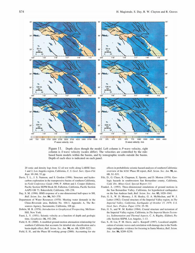
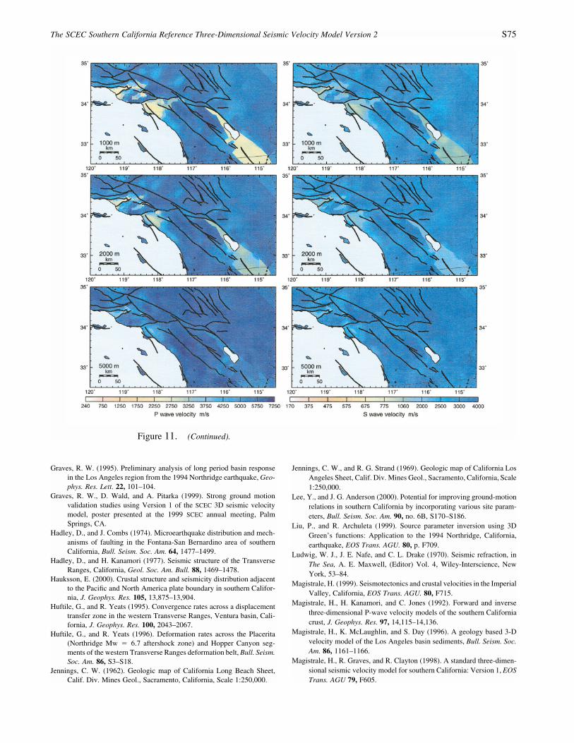
Figure 11. Depth slices though the model. Left column is P-wave velocity, rightcolumn is S-wave velocity (scales differ). The velocities are controlled by the rule-based basin models within the basins, and by tomographic results outside the basins.Depth of each slice is indicated on each panel.

20 sonic and density logs from 12 oil test wells along LARSE lines1 and 2, Los Angeles region, California, U. S. Geol. Surv. Open-FileRept. 98-366, 53 pp.

Davis, T. L., J. S. Namson, and S. Gordon (1996). Structure and hydro-carbon exploration in the transpressive basins of southern California,in Field Conference Guide 1996, P. Abbott and J. Cooper (Editors),Pacific Section SEPM Book 80, Fullerton, California, Pacific SectionAAPG GB 73, Bakersfield, California, 189–238.

Day, S. M. (1996). RMS response of a one-dimensional half-space to SH,Bull. Seism. Soc. Am. 86, 363–370.

Department of Water Resources (1970). Meeting water demands in theChino-Riverside area, Bulletin No. 104-3, Appendix A, The Re-sources Agency, Sacramento, California, 108 pp.

Dobrin, M. B. (1976). Introduction to Geophysical Prospecting, McGraw-Hill, New York.

Faust, L. Y. (1951). Seismic velocity as a function of depth and geologictime, Geophysics 16, 192–206.

Field, E. H. (2000). A modified ground-motion attenuation relationship forsouthern California that accounts for detailed site classification and abasin-depth effect, Bull. Seism. Soc. Am. 90, no. 6B, S209–S221.

Field, E. H., and the Phase III working group (2000). Accounting for site

effects in probabilistic seismic hazard analyses of southern California:overview of the SCEC Phase III report, Bull. Seism. Soc. Am. 90, no.6B, S1–S31.

Fife, D., G. Chase, R. Chapman, E. Sprotte, and D. Morton (1976). Geo-logic hazards in southwestern San Bernardino county, California,Calif. Div. Mines Geol. Special Report 113.

Frankel, A. (1993). Three-dimensional simulations of ground motions inthe San Bernardino Valley, California, for hypothetical earthquakeson the San Andreas fault, Bull. Seism. Soc. Am. 83, 1020–1041.

Fuis, G. S., W. D. Mooney, J. H. Healey, G. A. McMechan, and W. J.Lutter (1982). Crustal structure of the Imperial Valley region, in TheImperial Valley, California, Earthquake of October 15, 1979, U.S.Geol. Surv. Profess. Paper 1254, 25–50.

Fuis, G. S., and W. M. Kohler (1984). Crustal structure and tectonism ofthe Imperial Valley region, California, in The Imperial Basin-Tecton-ics, Sedimentation and Thermal Aspects, C. A. Rigsby, (Editor), Pa-cific Section SEPM, Los Angeles, 1–13.

Gao, S., H. Liu, P. M. Davis, and L. Knopoff (1997). Localized amplifi-cation of seismic waves and correlation with damage due to the North-ridge earthquake: evidence for focusing in Santa Monica, Bull. Seism.Soc. Am. 86, S209–S230.

The SCEC Southern California Reference Three-Dimensional Seismic Velocity Model Version 2 S75

Figure 11. (Continued).

Graves, R. W. (1995). Preliminary analysis of long period basin responsein the Los Angeles region from the 1994 Northridge earthquake, Geo-phys. Res. Lett. 22, 101–104.

Graves, R. W., D. Wald, and A. Pitarka (1999). Strong ground motionvalidation studies using Version 1 of the SCEC 3D seismic velocitymodel, poster presented at the 1999 SCEC annual meeting, PalmSprings, CA.

Hadley, D., and J. Combs (1974). Microearthquake distribution and mech-anisms of faulting in the Fontana-San Bernardino area of southernCalifornia, Bull. Seism. Soc. Am. 64, 1477–1499.

Hadley, D., and H. Kanamori (1977). Seismic structure of the TransverseRanges, California, Geol. Soc. Am. Bull. 88, 1469–1478.

Hauksson, E. (2000). Crustal structure and seismicity distribution adjacentto the Pacific and North America plate boundary in southern Califor-nia, J. Geophys. Res. 105, 13,875–13,904.

Huftile, G., and R. Yeats (1995). Convergence rates across a displacementtransfer zone in the western Transverse Ranges, Ventura basin, Cali-fornia, J. Geophys. Res. 100, 2043–2067.

Huftile, G., and R. Yeats (1996). Deformation rates across the Placerita(Northridge Mw � 6.7 aftershock zone) and Hopper Canyon seg-ments of the western Transverse Ranges deformation belt, Bull. Seism.Soc. Am. 86, S3–S18.

Jennings, C. W. (1962). Geologic map of California Long Beach Sheet,Calif. Div. Mines Geol., Sacramento, California, Scale 1:250,000.

Jennings, C. W., and R. G. Strand (1969). Geologic map of California LosAngeles Sheet, Calif. Div. Mines Geol., Sacramento, California, Scale1:250,000.

Lee, Y., and J. G. Anderson (2000). Potential for improving ground-motionrelations in southern California by incorporating various site param-eters, Bull. Seism. Soc. Am. 90, no. 6B, S170–S186.

Liu, P., and R. Archuleta (1999). Source parameter inversion using 3DGreen’s functions: Application to the 1994 Northridge, California,earthquake, EOS Trans. AGU. 80, p. F709.

Ludwig, W. J., J. E. Nafe, and C. L. Drake (1970). Seismic refraction, inThe Sea, A. E. Maxwell, (Editor) Vol. 4, Wiley-Interscience, NewYork, 53–84.

Magistrale, H. (1999). Seismotectonics and crustal velocities in the ImperialValley, California, EOS Trans. AGU. 80, F715.

Magistrale, H., H. Kanamori, and C. Jones (1992). Forward and inversethree-dimensional P-wave velocity models of the southern Californiacrust, J. Geophys. Res. 97, 14,115–14,136.

Magistrale, H., K. McLaughlin, and S. Day (1996). A geology based 3-Dvelocity model of the Los Angeles basin sediments, Bull. Seism. Soc.Am. 86, 1161–1166.

Magistrale, H., R. Graves, and R. Clayton (1998). A standard three-dimen-sional seismic velocity model for southern California: Version 1, EOSTrans. AGU 79, F605.

S76 H. Magistrale, S. Day, R. W. Clayton and R. Graves

Martin, G. (1994). Proceedings of the NCEER/SEAOC/BSSC Workshopon site response during earthquakes and seismic code provisions No-vember 18–20, University of Southern California Los Angeles.

McCulloh, T. H. (1960). Gravity variations and the geology of the LosAngeles basin of California, U.S. Geol. Surv. Profess. Paper 400-B,320–325.

Mooney, W. D., and G. A. McMechan (1982). Synthetic seismogram mod-eling for the laterally varying structure in the Imperial Valley, in TheImperial Valley, California, Earthquake of October 15, 1979, U.S.Geol. Surv. Profess. Paper 1254, 101–108.

Nafe, J. E., and C. L. Drake (1960). Physical properties of marine sedi-ments, in The Sea, M. N. Hill, (Editor) Vol. 3. Interscience, NewYork, 794–815.

Namson, J., and T. Davis (1992). Late Cenozoic thrust ramps of southernCalifornia, Final Report to the Southern California Earthquake Centerfor 1991 Contract, Davis & Namson Consulting Geologists, Valencia,California.

Olsen, K. B. (2000). Site amplification in the Los Angeles basin from three-dimensional modeling of ground motion, Bull. Seism. Soc. Am. 90,no. 6B, S77–S94.

Olsen, K. B., R. J. Archuleta, and J. R. Matarese (1996). Three-dimensionalsimulation of a magnitude 7.75 earthquake on the San Andreas fault,Science 270, 1628–1632.

Parsons, T., and J. McCarthy (1996). Crustal and upper mantle velocitystructure of the Salton trough, southeast California, Tectonics 15,456–471.

Rogers, T. H. (1965). Geologic map of California Santa Ana Sheet, Calif.Div. Mines Geol., Sacramento, California, Scale 1:250,000.

Rogers, T. H. (1967). Geologic map of California San Bernardino Sheet,Calif. Div. Mines Geol., Sacramento, California, Scale 1:250,000.

Roy, M., and R. Clayton (1999). Crust and mantle structure beneath theLos Angeles basin and vicinity: constraints from gravity and seismicvelocities, EOS Trans. AGU 80, F251.

Silva, W., S. Li, R. Darragh, and N. Gregor (1999). Surface geology basedstrong motion amplification factors for the San Francisco Bay andLos Angeles areas, P.G. & E. PEER Task 5.B Final Report, PacificEngineering and Analysis, El Cerrito, California, 109 pp.

Steidl, J. (2000). Site response in southern California for probabilistic seis-mic hazard analysis, Bull. Seism. Soc. Am. 90, no. 6B, S149–S169.

Tsutsumi, H., and R. Yeats (1999). Geologic setting of the 1971 San Fer-nando and 1994 Northridge earthquakes in the San Fernando Valley,California, J. Geophys. Res. (submitted).

Yeats, R., G. Huftile, and F. Grigsby (1988). Oak Ridge fault, Ventura foldbelt, and the Sisar decollement, Ventura basin, California, Geology16, 1112–1116.

Yeats, R., G. Huftile, and L. Stitt (1994). Late Cenozoic tectonics of theeast Ventura basin, Transverse Ranges, California, AAPG Bull. 78,1040–1074.

Yerkes, R. F., T. H. McCulloh, J. E. Schoellhamer, and J. G. Vedder (1965).Geology of the Los Angeles basin, California: an introduction, U.S.Geol. Surv. Profess. Paper 420-A, 1–57.

Wald, D., and R. Graves (1998). The seismic response of the Los Angelesbasin, California, Bull. Seism. Soc. Am. 88, 337–356.

Wessel, P., and W. H. K. Smith (1991). Free software helps map and displaydata, EOS 72, 445–446.

Wills, C. J., M. Petersen, W. A. Bryant, M. Reichle, G. J. Saucedo, S. Tan,G. Taylor, and J. Treiman (2000). A site-conditions map for Californiabased on geology and shear wave velocity, Bull. Seism. Soc. Am. 90,no. 6B, S187–S208.

Wright, T. L. (1991). Structural geology and tectonic evolution of the LosAngeles basin, California, AAPG Memoir 52, 35–134.

Zhou, H. (1994). Rapid three-dimensional hypocentral determination usinga master station method, J. Geophys. Res. 99, 15,439–15,456.

Zhu, L., and H. Kanamori (2000). Moho depth variation in southern Cali-fornia from teleseismic receiver functions, J. Geophys. Res. 105,2969–2980.

Department of Geological SciencesSan Diego State UniversitySan Diego, CA 92182-1020

(H. M., S. D.)

Seismological Laboratory 252-21California Institute of TechnologyPasadena, CA 91125

(R. W. C.)

URS Greiner Woodward Clyde566 El Dorado StreetPasadena, CA 91101

(R. G.)

Manuscript received 28 July 2000