Seismic dip estimation based on the

two-dimensional Hilbert transform and its

application in random noise attenuationa

aPublished in Applied Geophysics, 12, 55-63 (March 2015)

Cai Liu∗, Changle Chen∗, Dian Wang‡∗, Yang Liu∗, Shiyu Wang∗, and LiangZhang†

ABSTRACT

In seismic data processing, random noise seriously affects the seismic data qualityand subsequently the interpretation. This study aims to increase the signal-to-noise ratio by suppressing random noise and improve the accuracy of seismic datainterpretation without losing useful information. Hence, we propose a structure-oriented polynomial fitting filter. At the core of structure-oriented filtering isthe characterization of the structural trend and the realization of nonstationaryfiltering. First, we analyze the relation of the frequency response between two-dimensional (2D) derivatives and the 2D Hilbert transform (Riesz transform).Then, we derive the noniterative seismic local dip operator using the 2D Hilberttransform to obtain the structural trend. Second, we select polynomial fittingas the nonstationary filtering method and expand the application range of thenonstationary polynomial fitting. Finally, we apply variableamplitude polynomialfitting along the direction of the dip to improve the adaptive structureorientedfiltering. Model and field seismic data show that the proposed method suppressesthe seismic noise while protecting structural information.

INTRODUCTION

Random noise, which refers to any unwanted features in data, commonly contami-nates seismic data. Random noise sources in seismic exploration are roughly dividedinto three categories. First, there are external disturbances such as wind and humanactivities. Second, there is electronic instrument noise. Third, there is the irregularinterference owing to seismic explosions. Random noise attenuation is a significantstep in seismic data processing. In particular, the extent of noise suppression inpoststack data directly affects the accuracy of subsequent processing and interpreta-tion. Presently, several different random noise attenuation methods are available. Liu

∗College of Geo-exploration Science and Technology, Jilin University, Changchun 130026, China.†Qian An Oil Factory, Jilin Oilfield, CNPC, Songyuan 138000, China.‡Corresponding Author: Dian Wang (Email: dianwang@jlu.edu.cn)

Liu et al. 2 Dip estimation using Riesz transform

et al. (2006) presented a 2D multilevel median filter for random noise attenuation,whereas Liu et al. (2009b) used a 1D time-varying window median filter. Bekaraand van der Baan (2009) used the empirical mode decomposition (EMD) methodand proposed a filtering technique for random noise attenuation in seismic data. Liuet al. (2009a) proposed a high-order seislet transform for random noise attenuation.Li et al. (2012) applied morphological component analysis to suppress random noiseand Liu et al. (2012) proposed a novel method of random noise attenuation based onlocal frequency-domain singular value decomposition (SVD). Maraschini and Turton(2013) assessed the effect of nonlocal means random noise attenuator on coherency.Li et al. (2013) used time-frequency peak filtering to suppress strong noise in seis-mic data. Liu and Chen (2013) used f-x regularized nonstationary autoregression tosuppress random noise in 3D seismic data. The abovementioned random noise at-tenuation methods are limited by their lack of protection of structural information.For example, improper filtering may blur small faults, which may also make the dis-placement of larger fault continuous and consequently make layers appear continuousinstead of faulted. Obviously, this hinders fault interpretation, and makes denoisingand protecting structural information important. Fehmers and Hocker (2003) appliedstructureoriented filtering to fast structural interpretation. Hoeber et al. (2006) ap-plied nonlinear filters, such as median, trimmed mean, and adaptive Gaussian, overplanar surfaces parallel to the structural dip. Fomel and Guitton (2006) suggestedthe method of plane-wave construction by using model reparameterization. Liu et al.(2010) applied nonlinear structure-enhancing filtering by using plane-wave predictionto preserve structural information. Liu et al. (2011b) proposed a poststack randomnoise attenuation method by using weighted median filter based on local correlationand tried to balance the protection of fault information and noise attenuation.

Structure-oriented filtering includes structure prediction and filtering. Seismicdip is at the core of structure prediction; for, we can use seismic dip to determinestructural trends and achieve structure protection. Ottolini (1983) used local slantstack to formulate a local seismic dip estimation method. Fomel (2002) proposeda seismic dip estimation method based on the plane-wave destruction (PWD) filter.Schleicher et al. (2009) compared different methods of local dip computations. Theselection of filtering methods in structure-oriented filters is critical and polynomialfitting has been successfully applied to seismic data denoising. Lu and Lu (2009) usededge-preserving polynomial fitting to suppress random seismic noise. This methodachieves better results when the trajectories of seismic events are linear or the am-plitudes along the trajectories are not constant. Liu et al. (2011a) proposed a novelseismic noise attenuation method by using nonstationary polynomial fitting (Fomel,2009) and shaping regularization (Fomel, 2007) for constraining the smoothness ofthe polynomial coefficients.

In this paper, we discuss the two-dimensional (2D) Hilbert transform and use itto derive the formula for the dip in the plane wave, construct a stable algorithmfor estimating the dip, and improve the computational efficiency of Fomel’s method(Fomel, 2002) without minimizing the precision of the dip estimation. Finally, weuse synthetic model and field seismic data to demonstrate the applicability of the

Liu et al. 3 Dip estimation using Riesz transform

proposed method.

THEORY

The extraction of structural information and the selection of effective filtering meth-ods are critical to structure-oriented filters. Because of the time-space relation inseismic data, structural information must satisfy kinematics and kinetics equations.The dip of seismic events reveals structural features. This study is the first to discussa calculation method for the local seismic dip.

Noniterative local dip calculation

Following the local plane-wave equation (Fomel, 2002)

∂P (x, t)

∂x+ σ(x, t)

∂P (x, t)

∂t= 0, (1)

we define the local dip of seismic data

σ(x, t) = −∂P (x, t)

∂x/∂P (x, t)

∂t, (2)

where P (x, t) is the seismic wave field and σ(x, t) is the local seismic dip as a functionof time t and distance x. However, in actual computations, because the local dip isused to determine the direction of a seismic event, we ignore the dimensions and sam-pling interval; thus, σ only depends on the sampling data and the local dimensionlessdip is defined as

σ = −(∂P (x, t)

∂x/∂P (x, t)

∂t) · ∆x

∆t= −∂P

∂x/∂P

∂y, (3)

where ∂P/∂x and ∂P/∂y are the partial derivatives of the seismic wave field in the x−and y−direction, respectively, and ∆x and ∆t are the respective sampling intervalsin the x− and y−direction.

Using equation 3, we compute the local dip by using the specific values of thespace- and time-directional derivatives. Hence, we first discuss the derivative opera-tor.

The ideal differentiator frequency response is

FIDD(ω) = iω,−π ≤ ω ≤ π. (4)

The ideal differentiator frequency response is multiplied by a frequency-dependentlinear function in the frequency domain. The direct calculation of the derivativeof the signal in the time domain enhances the high-frequency random noise and

Liu et al. 4 Dip estimation using Riesz transform

reduces the dip accuracy. Thus, we analyze the frequency response of the derivativeoperator and the frequency response of the Hilbert transform. We derive the Hilberttransform (Appendix A) and the approximate partial derivative by using the finiteimpulse response (FIR) filter (Pei and Wang, 2001). We use a 2D Hilbert transformto approximate the partial derivatives of the wave field, which reduces the side effectof strong high-frequency random noise owing to the derivative algorithm.

The redefined noniterative local dip of the seismic data is

σ = −(∂P

∂x/∂P

∂y) = −FFT

−1[P (x)]

FFT−1[P (y)]= −

FFT−1[ 1√cxP (x)]

FFT−1[ 1√cyP (y)]

≈−FFT−1[HHT (x)]

FFT−1[HHT (y)]≈−HHTx

HHTy

,

(5)where P (x) is the frequency response function of the partial derivative in the x−directionand P (y) is the frequency response function of the partial derivative in the y−direction.The dimensions are ignored in the derivation and c does not depend on the time andspace sampling intervals; thus, we take cx = cy. HHT (x) is the frequency responsefunction of the Hilbert transform in the x−direction and HHT (y) is the frequencyresponse function of the Hilbert transform in the y−direction. HHTx and HHTy arethe components of the 2D Hilbert transform in the x− and y−direction, respectively.Using equation 5, we calculate the local seismic dip attribute by using the 2D Hilberttransform instead of the derivative operation. Because division is required in equa-tion 5 and the denominator might become zero, we add the nonzero constant ε in thedenominator

σ≈− HHTx

HHTy + ε. (6)

Fomel (2007) proposed the shaping regularization for imposing regularization con-straints in estimation problems and defined the local seismic attributes. In this paper,we use the same method to constrain the division and smooth the local dip by usingthe Gaussian smooth operator as the regularization operator.

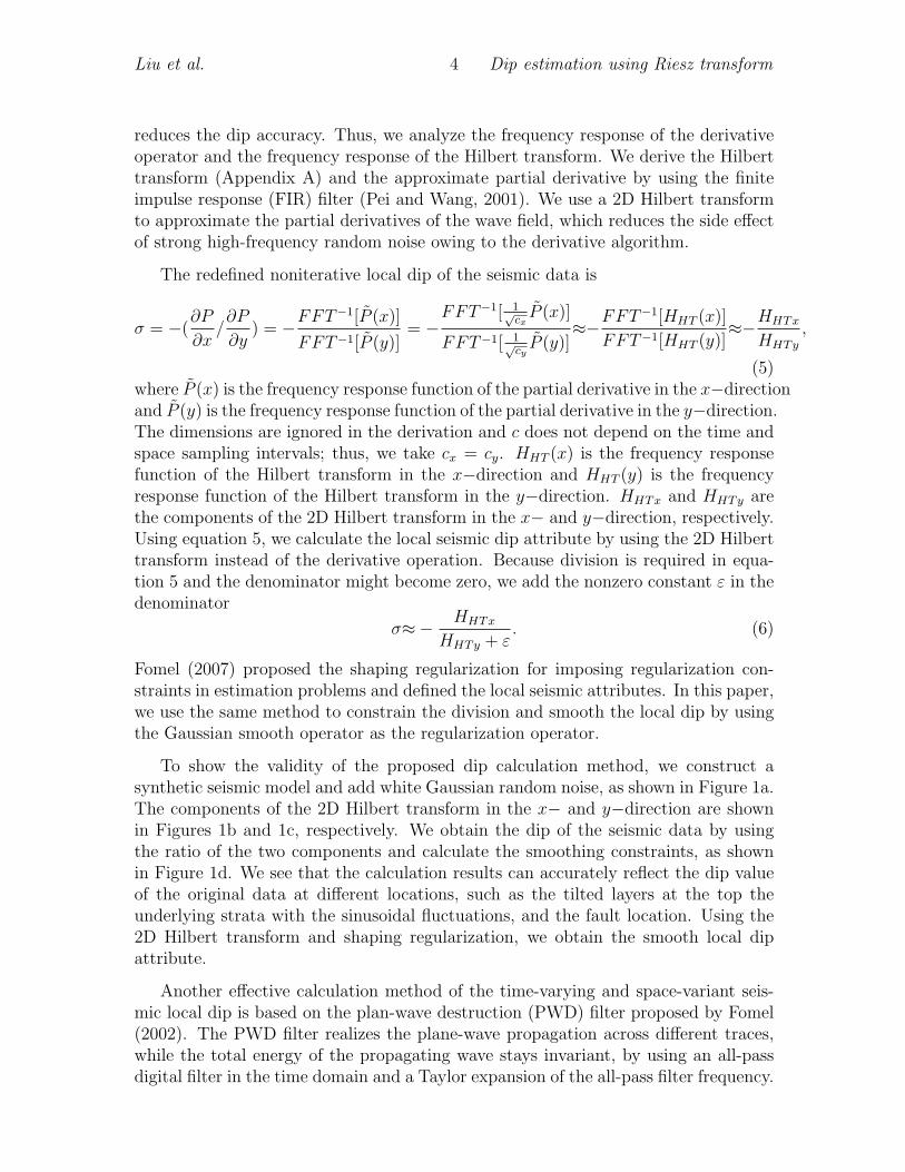
To show the validity of the proposed dip calculation method, we construct asynthetic seismic model and add white Gaussian random noise, as shown in Figure 1a.The components of the 2D Hilbert transform in the x− and y−direction are shownin Figures 1b and 1c, respectively. We obtain the dip of the seismic data by usingthe ratio of the two components and calculate the smoothing constraints, as shownin Figure 1d. We see that the calculation results can accurately reflect the dip valueof the original data at different locations, such as the tilted layers at the top theunderlying strata with the sinusoidal fluctuations, and the fault location. Using the2D Hilbert transform and shaping regularization, we obtain the smooth local dipattribute.

Another effective calculation method of the time-varying and space-variant seis-mic local dip is based on the plan-wave destruction (PWD) filter proposed by Fomel(2002). The PWD filter realizes the plane-wave propagation across different traces,while the total energy of the propagating wave stays invariant, by using an all-passdigital filter in the time domain and a Taylor expansion of the all-pass filter frequency.

Liu et al. 5 Dip estimation using Riesz transform

a b

c d

Figure 1: Local seismic dip based on the 2D Hilbert transform. Synthetic seismicdata (a), time component of the 2D Hilbert transform (b), space component of the2D Hilbert transform (c), and local seismic dip (d).

Liu et al. 6 Dip estimation using Riesz transform

We obtain the relation of the PWD and space-time-varying local seismic dip by usingthe Gauss-Newton algorithm to solve the nonlinear problem of local seismic dip. Thismethod can be essentially understood as solving an implicit finite-difference schemefor the local planewave equation. The disadvantage of the PWD-based calculationmethod is its slow computation speed, which is especially worse at higher order con-ditions. The computational cost of the proposed method is proportional to 2Nx×Nt,where Nx × Nt is the data size, whereas the computational efficiency of the PWD-based dip estimation method is proportional to Niter × Nx × Nt, where Niter is thenumber of iterations. Hence, to achieve similar accuracy, the dip estimation methodbased on the 2D Hilbert transform requires a smaller number of iterations than thePWD-based method.

The dip of seismic events controls the trend of the constructed seismic model;thus, next, we need to apply filtering along the trend. The selected filtering methodmust simultaneously suppress the seismic noise and protect structural information.

Nonstationary polynomial fitting

Traditional stationary regression is used to estimate the coefficients ai, i = 1, 2, . . . , Nby minimizing the prediction error between a “master” signal s(x) (where x representsthe coordinates of a multidimensional space) and a collection of slave signals Li(x), i =1, 2, . . . , N (Fomel, 2009)

E(x) = s(x)−N∑

i=1

aiLi(x). (7)

When x is 1D and N = 2, L1(x) = 1 and L2(x) = x , the problem of minimizingE(x) amounts to fitting a straight line a1 + a1x to the master signal. Nonstationaryregression is similar to equation 7 but allows the coefficients ai(x) to vary with x,and the error (Fomel, 2009)

E(x) = s(x)−N∑

i=1

ai(x)Li(x) (8)

is minimized to solve for the multinomial coefficients ai(x). The minimization be-comes an ill-posed problem because ai(x) rely on the independent variables x. Tosolve the ill-posed problem, we constrain the coefficients ai(x). Tikhonov’s regular-ization (Tikhonov, 1963) is a classical regularization method that amounts to theminimization of the following functional (Fomel, 2009)

F (a) = ‖E(x)‖2 + ε2

N∑i=1

‖D[ai(x)]‖2, (9)

where D is the regularization operator and ε is a scalar regularization parameter.When D is a linear operator, the least-squares estimation reduces to linear inversion

Liu et al. 7 Dip estimation using Riesz transform

(Fomel, 2009)a = A−1d, (10)

where

a = [a1(x)a2(x) · · · aN(x)]T ,

d = [L1(x)s(x)L2(x)s(x) · · ·LN(x)s(x)]T ,

and the elements of matrix A are

Aij(x) = Li(x)Lj(x) + ε2δijDT D .

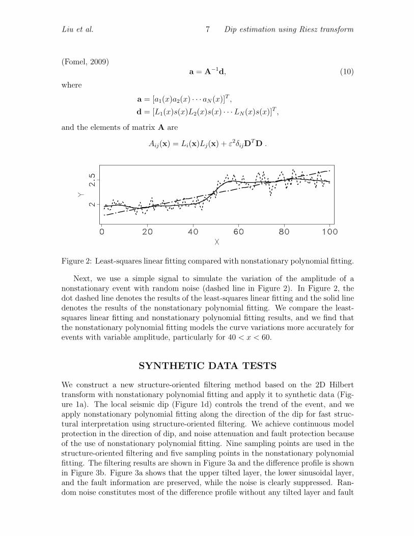
Figure 2: Least-squares linear fitting compared with nonstationary polynomial fitting.

Next, we use a simple signal to simulate the variation of the amplitude of anonstationary event with random noise (dashed line in Figure 2). In Figure 2, thedot dashed line denotes the results of the least-squares linear fitting and the solid linedenotes the results of the nonstationary polynomial fitting. We compare the least-squares linear fitting and nonstationary polynomial fitting results, and we find thatthe nonstationary polynomial fitting models the curve variations more accurately forevents with variable amplitude, particularly for 40 < x < 60.

SYNTHETIC DATA TESTS

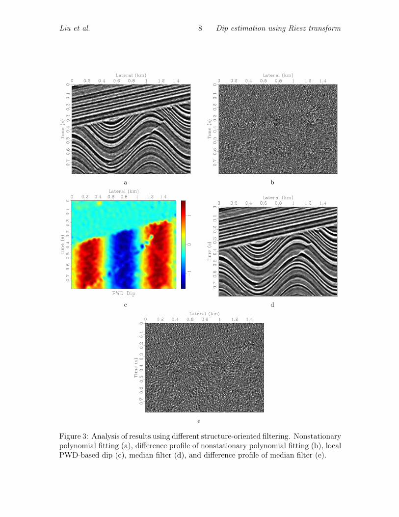
We construct a new structure-oriented filtering method based on the 2D Hilberttransform with nonstationary polynomial fitting and apply it to synthetic data (Fig-ure 1a). The local seismic dip (Figure 1d) controls the trend of the event, and weapply nonstationary polynomial fitting along the direction of the dip for fast struc-tural interpretation using structure-oriented filtering. We achieve continuous modelprotection in the direction of dip, and noise attenuation and fault protection becauseof the use of nonstationary polynomial fitting. Nine sampling points are used in thestructure-oriented filtering and five sampling points in the nonstationary polynomialfitting. The filtering results are shown in Figure 3a and the difference profile is shownin Figure 3b. Figure 3a shows that the upper tilted layer, the lower sinusoidal layer,and the fault information are preserved, while the noise is clearly suppressed. Ran-dom noise constitutes most of the difference profile without any tilted layer and fault

Liu et al. 8 Dip estimation using Riesz transform

a b

c d

e

Figure 3: Analysis of results using different structure-oriented filtering. Nonstationarypolynomial fitting (a), difference profile of nonstationary polynomial fitting (b), localPWD-based dip (c), median filter (d), and difference profile of median filter (e).

Liu et al. 9 Dip estimation using Riesz transform

information left because the local seismic dip cannot reflect the trend of the layersand owing to the attenuation of the limited effective information. To compare theproposed method with the PWD-based local dip estimation method (Figure 3c) withsimilar dip accuracy (Figure 1d), we choose the median filter and show the results inFigure 3d and the difference profile in Figure 3e. We compare the two profiles afterthe application of the median filter. We find more useful structural information thanthe method we proposed. That means the method we proposed has better effect.

FIELD DATA TESTS

a b

c d

Figure 4: Comparison of processing results. Field data (a), Local dip (b), Afterfiltering (c), Difference profile (d).

For field data processing, we chose the 2D profile of 3D poststack data (Liu andChen, 2013). The shallow structures are simple planar layers and the deep structuresare complex curved layers. First, we use the proposed method, which is based onthe 2D Hilbert transform, to compute the corresponding local seismic dip attribute(Figure 4b). From Figure 4b, we see that the dip changes smoothly and steadily in

Liu et al. 10 Dip estimation using Riesz transform

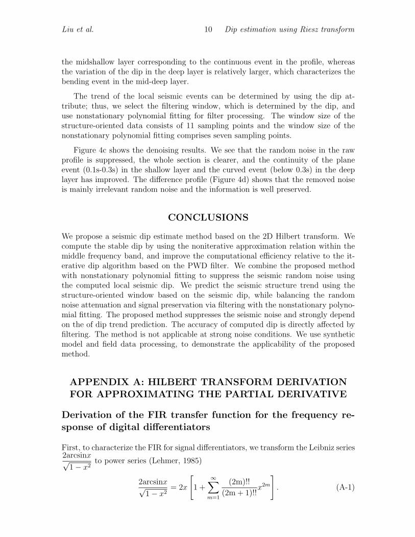
the midshallow layer corresponding to the continuous event in the profile, whereasthe variation of the dip in the deep layer is relatively larger, which characterizes thebending event in the mid-deep layer.

The trend of the local seismic events can be determined by using the dip at-tribute; thus, we select the filtering window, which is determined by the dip, anduse nonstationary polynomial fitting for filter processing. The window size of thestructure-oriented data consists of 11 sampling points and the window size of thenonstationary polynomial fitting comprises seven sampling points.

Figure 4c shows the denoising results. We see that the random noise in the rawprofile is suppressed, the whole section is clearer, and the continuity of the planeevent (0.1s-0.3s) in the shallow layer and the curved event (below 0.3s) in the deeplayer has improved. The difference profile (Figure 4d) shows that the removed noiseis mainly irrelevant random noise and the information is well preserved.

CONCLUSIONS

We propose a seismic dip estimate method based on the 2D Hilbert transform. Wecompute the stable dip by using the noniterative approximation relation within themiddle frequency band, and improve the computational efficiency relative to the it-erative dip algorithm based on the PWD filter. We combine the proposed methodwith nonstationary polynomial fitting to suppress the seismic random noise usingthe computed local seismic dip. We predict the seismic structure trend using thestructure-oriented window based on the seismic dip, while balancing the randomnoise attenuation and signal preservation via filtering with the nonstationary polyno-mial fitting. The proposed method suppresses the seismic noise and strongly dependon the of dip trend prediction. The accuracy of computed dip is directly affected byfiltering. The method is not applicable at strong noise conditions. We use syntheticmodel and field data processing, to demonstrate the applicability of the proposedmethod.

APPENDIX A: HILBERT TRANSFORM DERIVATIONFOR APPROXIMATING THE PARTIAL DERIVATIVE

Derivation of the FIR transfer function for the frequency re-sponse of digital differentiators

First, to characterize the FIR for signal differentiators, we transform the Leibniz series2arcsinx√

1− x2to power series (Lehmer, 1985)

2arcsinx√1− x2

= 2x

[1 +

∞∑m=1

(2m)!!

(2m + 1)!!x2m

]. (A-1)

Liu et al. 11 Dip estimation using Riesz transform

We substitute sin(ω

2) for x, and after rearrangement and truncation of the first M

terms, we obtain

ω√1− sin2ω

2

= 2sinω

2

[1 +

M∑m=1

(2m)!!

(2m + 1)!!

(1− cosω

2

)m

+ o((1− cosω

2)M+1)

] (A-2)

and after manipulation

ω = 2sinω

2cos

ω

2

[1 +

M∑m=1

(2m)!!

(2m + 1)!!

(1− cosω

2

)m

+ o((1− cosω

2)M+1)

]

= sinω

[1 +

M∑m=1

(2m)!!

(2m + 1)!!

(1− cosω

2

)m

+ o((1− cosω

2)M+1)

].

(A-3)

We ignore the higher order terms and we obtain the (2M + 2)th-order causal transferfunction of the derivative operator as

FDD(z) ≈ −1− z−2

2

{z−M +

M∑m=1

(2m)!!

(2m + 1)!!·z−(M−m)

[−(1− z−1)2

4

]m}. (A-4)

Derivation of the FIR transfer function for the frequency re-sponse of the Hilbert transform

The ideal frequency response of the Hilbert transform is expressed as

HIHT (ω) = −i sgnω = −i ω|ω|

=

{i, −π < ω < 0−i, 0 < ω < π

. (A-5)

From equations 4 and A-5, we obtain the difference as 1/ |ω|. For

sgnx =x√x2

= xf(x2), x 6= 0 (A-6)

and f(u) =1√u, u > 0, the Taylor series of f(u) at center c is expressed

f(u) =1√c

[1 +

∞∑m=1

(2m− 1)!!

(2m)!!

(1− u

c

)m], (A-7)

where (2m− 1)!! = 1 · 3 · 5 . . . (2m− 1), (2m)!! = 1 · 3 · 5 . . . (2m). Consequently, thesignum function sgnx is expressed

sgnx =x√c

[1 +

∞∑m=1

(2m− 1)!!

(2m)!!

(1− x2

c

)m]. (A-8)

Liu et al. 12 Dip estimation using Riesz transform

We substitute sinω for x, based on sgnω=sgn(sinω) for π < ω < π, truncate the seriesat the first M terms, and obtain the sinusoidal power series of the signum function as

sgnω =sinω√

c

[1 +

M∑m=1

(2m− 1)!!

(2m)!!

(1− sin2ω

c

)m

+ ◦((1− sin2ω

c)M+1)

](A-9)

The series in A-9 converges for −1 < 1− sinω

c< 1; that is, c has to be larger than

1/2. On the other hand, the expansion center c in the x-domain is associated to thefrequency center in the ω-domain via the relation c = sin2ωc. Therefore, c = sin2ωc

must be less than or equal to 1. Accordingly, c is constrained by 1/2 < c ≤ 1 and thecorresponding ωc is within the range [π/4, π/2]. Clearly, the ideal frequency responseis well approximated within the middle frequency band. Multiplying A-9 by −i and

substitutingz − z−1

2ifor sinω, the transfer function for the zero phase FIR of the

Hilbert transform is expressed as

HHT (z, c) ≈ −z− z−1

2√

c

{1 +

M∑m=1

(2m− 1)!!

(2m)!!

[1 +

1

c

(z− z−1

2

)2]m}

(A-10)

To obtain the causal transfer function, HHT (z, c) is multiplied by z−2M−1 and theresultant transfer function of the FIR Hilbert transform of the (2M+2)th-order is

HHT (z, c) ≈ −1− z−2

2√

c

{z−2M +

M∑m=1

(2m− 1)!!

(2m)!!z−2(M−m)

[z−2 +

1

c

(1− z−2

2

)2]m}(A-11)

For M=0, the transfer functions of equations A-4 and A-11 are approximated as

HHT (z, c) ≈ −1− z−2

2√

c(A-12)

FDD(z) ≈ −1− z−2

2(A-13)

We compare equations A-12 and A-13, and we conclude that these two transfer func-tions in middle frequency band of the frequency domain differ by the constant coef-

ficient1√c.

REFERENCES

Bekara, M., and M. van der Baan, 2009, Random and coherent noise attenuation byempirical mode decomposition: Geophysics, 74, V89–V98.

Fehmers, G. C., and C. F. W. Hocker, 2003, Fast structural interpretation withstructure-oriented filtering: Geophysics, 68, 1286–1293.

Liu et al. 13 Dip estimation using Riesz transform

Fomel, S., 2002, Applications of plane-wave destruction filters: Geophysics, 67, 1946–1960.

——–, 2007, Shaping regularization in geophysicalestimation problems: Geophysics,72, R29–R36.

——–, 2009, Adaptive multiple subtraction using regularized nonstationary regres-sion: Geophysics, 74, V25–V33.

Fomel, S., and A. Guitton, 2006, Regularizing seismic inverse problems by modelreparameterization using plane-wave construction: Geophysics, 71, A43–A47.

Hoeber, H. C., S. Brandwood, and D. N. Whitcombe, 2006, Structurally consistentfiltering: In 68th EAGE Conference Exhibition.

Lehmer, D. C., 1985, Interesting series involving the central binomial coefficient:American Mathematical Monthly.

Li, H. S., G. C. Wu, and X. Y. Yin, 2012, Application of morphological compo-nent analysis to remove of random noise in seismic data: Journal of Jilin Univer-sity(Earth Science Edition), 42, 554–561.

Li, Y., B. J. Yang, and H. B. L. et al., 2013, Suppression of strong random noise inseismic data by using timefrequency peak filtering: Science China Earth Sciences,56, 1200–1208.

Liu, C., Y. Liu, B. J. Yang, D. Wang, and J. G. Sun, 2006, A 2D multistage medianfilter to reduce random seismic noise: Geophysics, 71, 105–110.

Liu, G., and X. Chen, 2013, Noncausal f-x-y regularized nonstationary predictionfiltering for random noise attenuation on 3d seismic data: Journal of Applied Geo-physics, 93, 60–66.

Liu, G. C., X. H. Chen, J. Y. Li, and et al., 2011a, Seismic noise attenuation usingnonstationary polynomial fitting: Applied Geophysics, 8, 18(C26.

Liu, Y., S. Fomel, C. Liu, and et al., 2009a, High-order seislet transform and itsapplication of random noise attenuation: Chinese Journal of Geophysics, 52, 2142–2151.

Liu, Y., S. Fomel, and G. Liu, 2010, Nonlinear structureenhancing filtering usingplane-wave prediction: Geophysical Prospecting, 58, 415–427.

Liu, Y., C. Liu, and D. Wang, 2009b, A 1D time-varying median filter for seismicrandom, spike-like noise elimination: Geophysics, 74, 17–24.

Liu, Y., D. Wang, and C. Liu, 2011b, Weighted median filter based on local correlationand its application to poststack random noise attenuation: Chinese Journal ofGeophysics, 54, 358–367.

Liu, Z., W. Zhao, and X. Chen, 2012, Local svd for random noise suppression ofseismic data in frequency domain: Oil Geophysical Prospecting, 47, 202–206.

Lu, Y. H., and W. K. Lu, 2009, Edge-preserving polynomial fitting method to suppressrandom seismic noise: Geophysics, 74, V69–V73.

Maraschini, M., and C. G. G. N. Turton, 2013, Assessing the impact of a non-local-means random noise attenuator on coherency: SEG Technical Program ExpandedAbstracts.

Ottolini, R., 1983, Signal/noise separation in dip space: SEP Report, 37.Pei, S. C., and P. H. Wang, 2001, Closed-form design of maximally flat fir hilbert

transformers, differentiators, and fractional delayers by power series expansion:

Liu et al. 14 Dip estimation using Riesz transform

IEEE Transactions on, Circuits and Systems I: Fundamental Theory and Applica-tions, 48, 389–398.

Schleicher, J., J. C. Costa, and L. T. Santos, 2009, On the estimation of local slopes:Geophysics, 74, P25–P33.

Tikhonov, A., 1963, Solution of incorrectly formulated problems and the regulariza-tion method: In Soviet Math.Dokl.