30
Final Report: Temporal Changes of La Parguera Reefs as Detected with Remote Sensing Ketlyn A. Rodríguez González 802-00-6394 Advisor: Dr. Fernando Gilbes
| Date post: | 04-Aug-2018 |
| Category: |
Documents |
| Upload: | truonghanh |
| View: | 217 times |
| Download: | 0 times |

Final Report: Temporal Changes of La Parguera Reefs
as Detected with Remote Sensing
Ketlyn A. Rodríguez González 802-00-6394
Advisor: Dr. Fernando Gilbes

Abstract The purpose of this research is the use of Remote Sensing to determine changes through
time of the distribution of the coral reefs of La Parguera. For this, three aerial photograph (1936,
1977, 1999) and two images (CASI, IKONOS) of the area were processed using IsoData, K-
Means and Minimum Distance methods. IsoData and K-Means results were not the best. The
Minimum Distance had the best results and changes through time in the distribution of the reefs
are detected. Remote Sensing, then, can be used to detect changes of the distribution of the coral
reefs of La Parguera.
Introduction
Coral reefs are considered to be the rain forest of the oceans due to its biodiversity.
Around 25 % of the world’s marine species are located in these ecosystems (CNN, 1997). Due to
anthropogenic and natural causes, coral reefs are in jeopardy. Human activities such as fishing,
sailing, costal development, agriculture, deforestation, among others, are responsible for most of
the coral reefs degradation (CoRIS, 2004).
Fishermen exploit coral reefs because of the diversity found in them. This over fishing
causes the overgrowth of sea grass. Since there is no sufficient fish to eat it, coral reefs get
covered with algae and can not receive enough sunlight needed for photosynthesis of the
Zooxanthellae that live in them and provide color and additional food for the corals (Ocean
World, 2004). Boats that pass by these ecosystems can affect them by breaking them apart and
by spilling their fuels, polluting the area. Construction of hotels and tourist’s developments
causes runoffs, sedimentation and sewage spills. Eventually these end in the ocean bringing high
amounts of nutrients and turbidity, decreasing the sun light that gets into water and causing
eutrophication (overgrowth of algae in water due to the excess of nutrients causing the go away
of the Zooxanthellae from the coral because they do not receive sufficient light for their
photosynthesis). Corals then bleach and can die (CoRIS, 2004).
Agriculture and deforestation have more or less the same effects on them. The chemicals
needed for maximum cultivation go to the coasts when it rains and eutrophicate the areas. When
there is a clear up of green areas, the land that used to be covered with grass, trees, plants, etc., is
no more protected or stable. Rain falls and the unprotected terrain mixes with the water carrying
sediments and nutrients to the coast.
Natural causes such as hurricanes, greenhouse gases, low tide, etc., also affect negatively
the coral reefs. The drastic rains, involving hurricanes, bring huge quantities of sediments that
end in the oceans and powerful waves, which can break corals apart. The greenhouse gases effect
warms the water. Zooxanthellae can not live in such temperature conditions and they leave the
corals. Then corals suffer from bleaching. Lowering in the tide rise can also cause bleaching.
Coral reefs are exposed receiving direct rays of light that expel the Zooxanthellae (CoRIS, 2004).
Corals reefs around the world are affected by these stresses and Puerto Rico’s coral reefs
are no exception. In this research the area of study is La Parguera in Lajas. The coral reefs in this
location are considered to be the healthiest of coastal Puerto Rico, because of their high
abundance of living coral. This is caused by some factors (Bruckner, A., Carlo, M., Morelock, J.,
Ramírez, W., 2001).
Mangroves are natural barriers that prevent sediments from being carried by the run offs
directly to reefs. There are no close rivers that could cause eutrophication and/or a lowering of
the sunrays into the water column due to sediments. These help to maintain certain healthy status
in the coral reefs. Anyhow, they are being affected by the rapid urbanization that increases the
sedimentation in rainy seasons, bringing nutrients from the terrain and the sewage systems,
increasing the growth of sea grass. Hurricanes also have been contributing to their degradation
due to the excess of sediments and their destructive waves (Bruckner, A., Carlo, M., Morelock,
J., Ramírez, W., 2001). Having all these factors in mind it is possible to come up with some ideas
for a research that could help to determine changes in the reefs of La Parguera.
Remote sensing can not determine which are exactly the reasons for the changes of the
reefs, but it is possible to infer what may have cause it by establishing the relation of the urban
development with the reefs changes. The sensors can detect construction and development of the
area (land use and land cover changes); and we could find out if these are being increasing by
comparing the images and photos. The urban development can cause run offs with sediments and
nutrients eutrophicating the reefs. This eutrophication may cause changes in the distribution
ecosystem.
Objectives
This research is concentrated in the study of the coral reefs of La Parguera from 1930’s to
present. Images of these reefs taken by IKONOS, CASI (Compact Airborne Spectrographic
Imager), and three aerial photos (1936, 1977 and 1999) were analyzed to see if there are visible
and spectral changes in the reefs. It tries to determine changes through time of the distribution of
the communities that compose the ecosystem. The research will find out if several remote
sensors can easily capture these changes and which is the best sensor for it. This will help to
select the right tool for future studies. Also, it pretends to determine whether or not there are

noticeable distribution differences in the spectral response in the reefs between the images and
photos, and which of the unsupervised (IsoData and K-Means) methods used to detect the
changes are similar to the supervised method. Therefore, the hypothesis of my work is that
remote sensing techniques can be used to detect the distribution changes of coral reef’s
communities through time.
Methodology
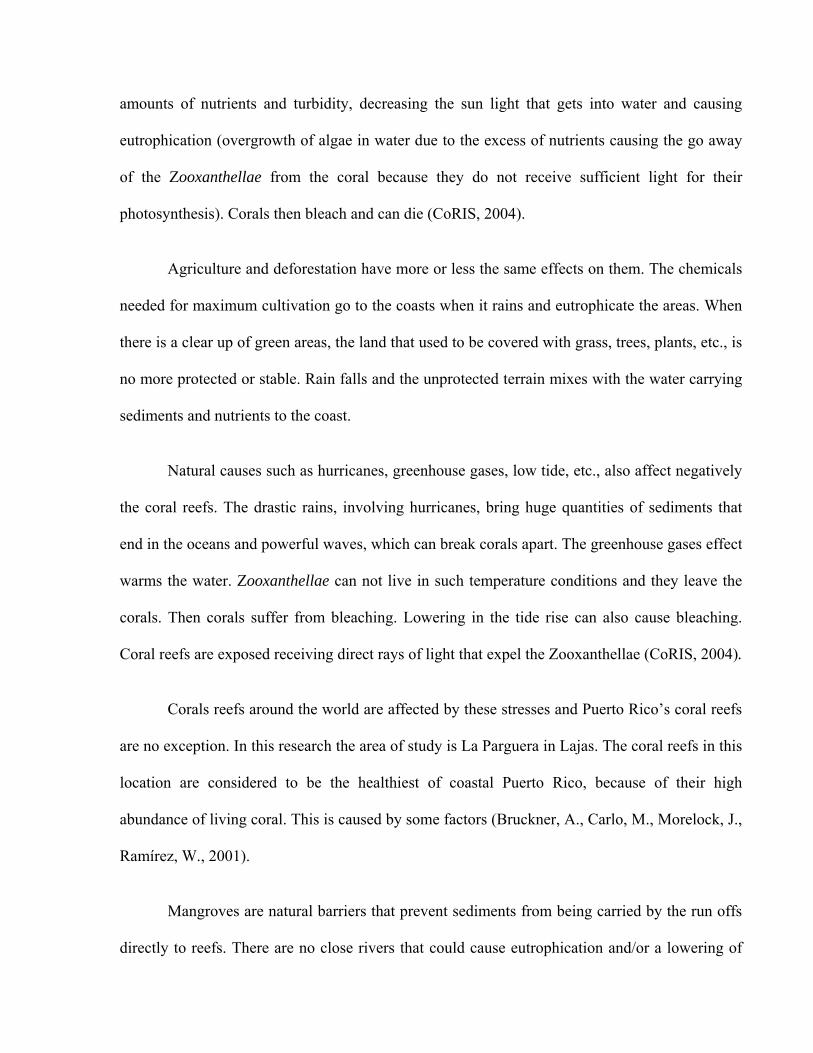
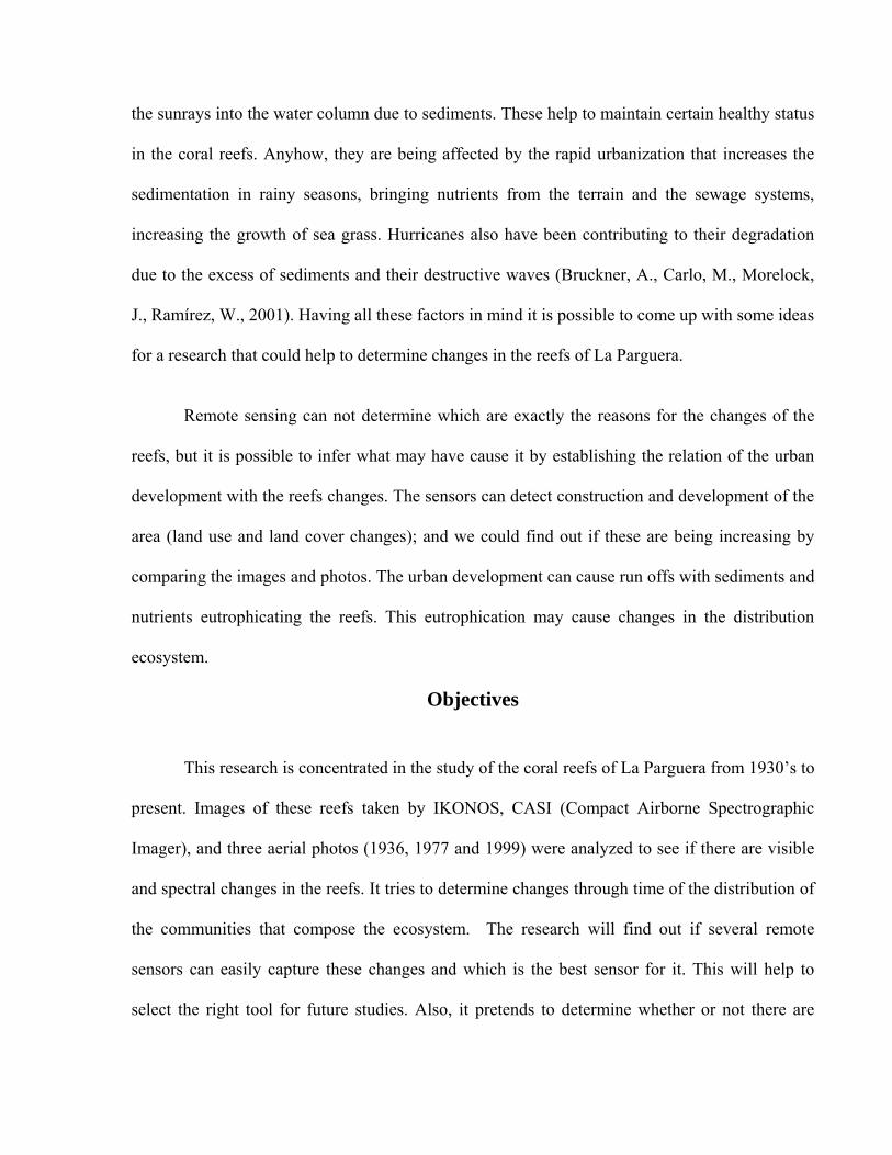
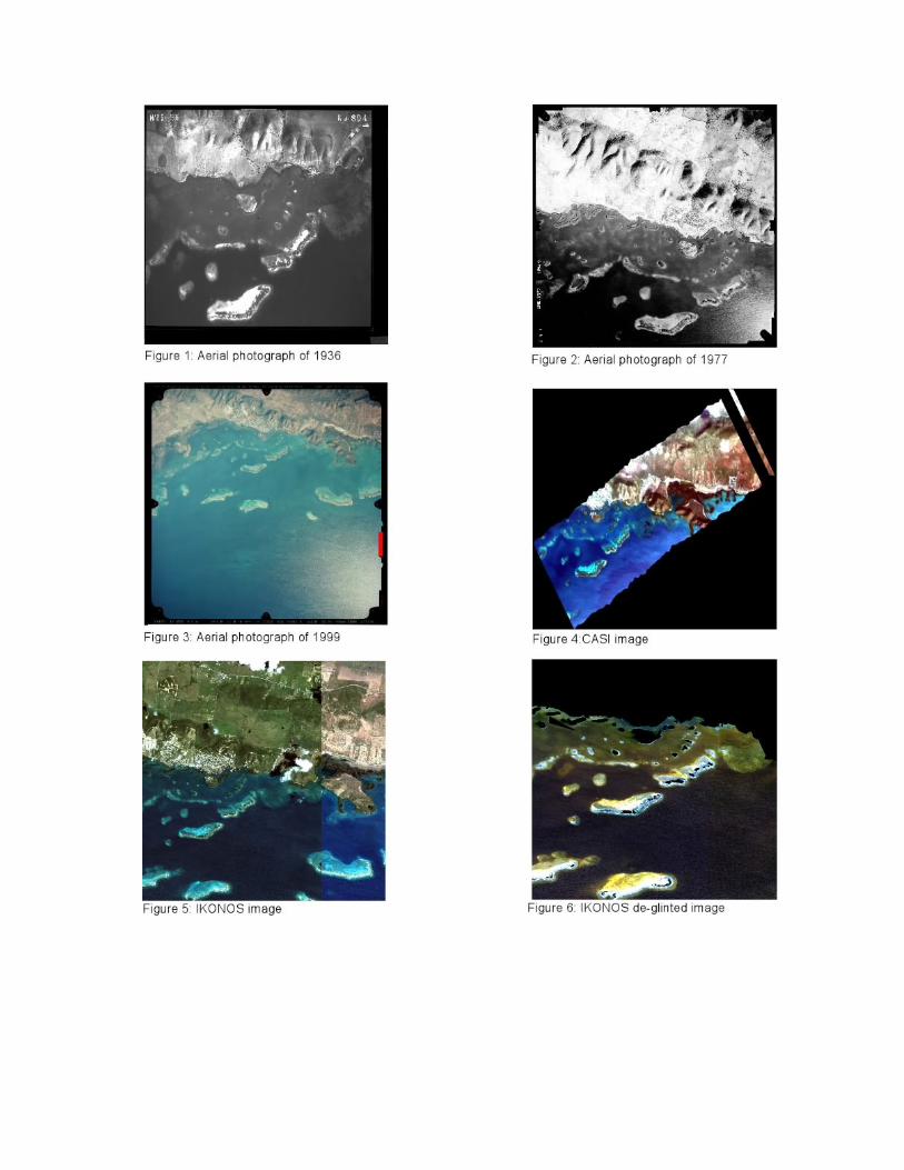
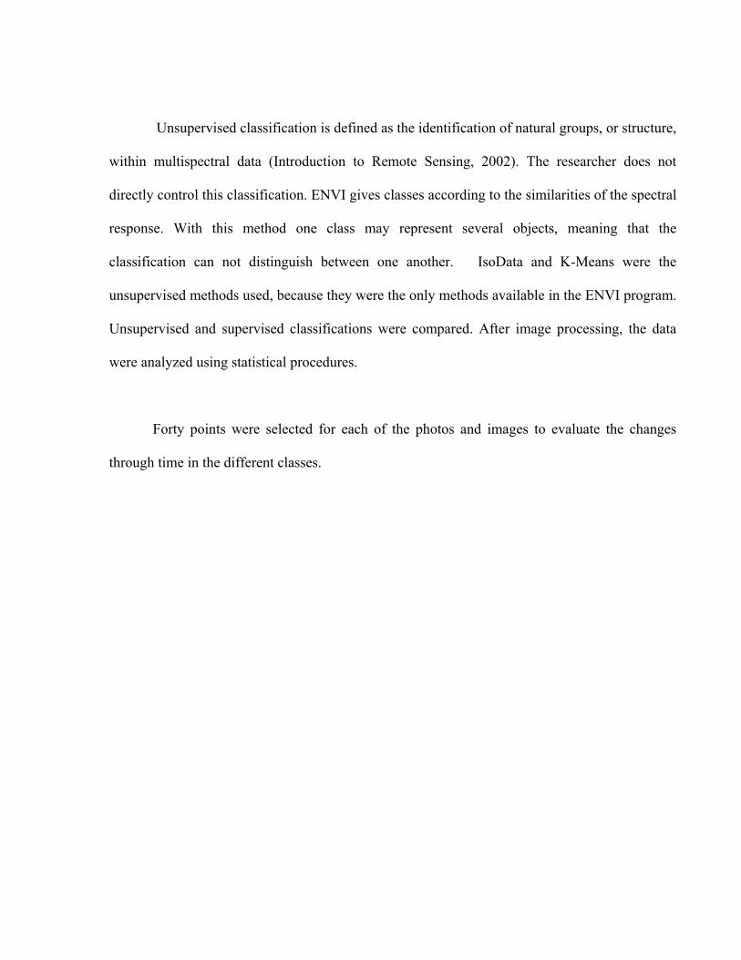
Three images of La Parguera, one from IKONOS without being pre-processed (Figure 5),
the other one a de-glinted IKONOS (figure 6), CASI (Figure 4) and aerial photograph from 1999
(figure 3) were facilitated by the GERS (Geological and Environmental Remote Sensing
Laboratory). Aerial photographs from 1936 (figure 1) and 1977 (figure 2) were provided by ¨La
División de Fotogrametría de la Autoridad de Carreteras¨. ENVI (Environmental of Visualization
Images) was the program used for the processing of the images and photos.
Table 1:IKONOS and CASI sensor descriptions Sensor Orbit Resolution Bands
IKONOS Sun synchronous, every 98 minutes
High spatial resolution (1m, 4m)
Panchromatic, multispectral
CASI Airborne combines the best of aerial photography and satellite imagery.
High spatial resolution (5m)
Hyperspectral 288 channels (400- 915
nm)

For the purpose of the investigation, IKONOS and CASI images with three aerial photos
of La Parguera reefs were processed using ENVI. There was a need to use a de-glinted IKONOS
image (figure 5) because the original one had sun glint problems that affected the outcome result
of the unsupervised images, not letting to identify the real classification in the water. The aerial
photos of different years (1936, 1977, and 1999) were compared in between and with the images
(image interpretation) to determine visible changes of the reefs. Georeferencing and atmospheric
corrections were performed. This is needed to have a better quality of the images and photos
classification. The CASI image (figure 10) and the aerial photos (figure 7, 8 & 9) were
georeferenced based on coordinates of the IKONOS image (figure 1), because it has the highest
spatial resolution. The de-glinted image was not georeferenced, because it was already.
Georeferencing consist in removing geometric errors and rectified to a real-world coordinate
system (Decision Support, 2003). After the georeferenciation, they were re-sized using the subset
application to have the same study area in all of them (figures: 11, 12, 13, 14,15 & 16).
Atmospheric corrections were done to correct atmospheric attenuation and some
scattering effects to obtain a close estimate of a surface spectral radiance (CIS, 2004). For these
atmospheric corrections the dark subtract method was applied to each of the images and aerial
photos, except for the de-glinted IKONOS that already was pre-processed with the de-glinted
method. Then, they were classified using supervised and unsupervised methods. Supervised
classification is defined as the processes using sample of known identity to classify pixels of
unknown data. The analysts have control of the data and they select the regions of interest
(ROIs), which are the areas that are going to be classified to distinguish one object from the
other. Minimum distance was the method used for this classification. It classifies using the ROI’s
closest pixels.
Unsupervised classification is defined as the identification of natural groups, or structure,
within multispectral data (Introduction to Remote Sensing, 2002). The researcher does not
directly control this classification. ENVI gives classes according to the similarities of the spectral
response. With this method one class may represent several objects, meaning that the
classification can not distinguish between one another. IsoData and K-Means were the
unsupervised methods used, because they were the only methods available in the ENVI program.
Unsupervised and supervised classifications were compared. After image processing, the data
were analyzed using statistical procedures.
Forty points were selected for each of the photos and images to evaluate the changes
through time in the different classes.


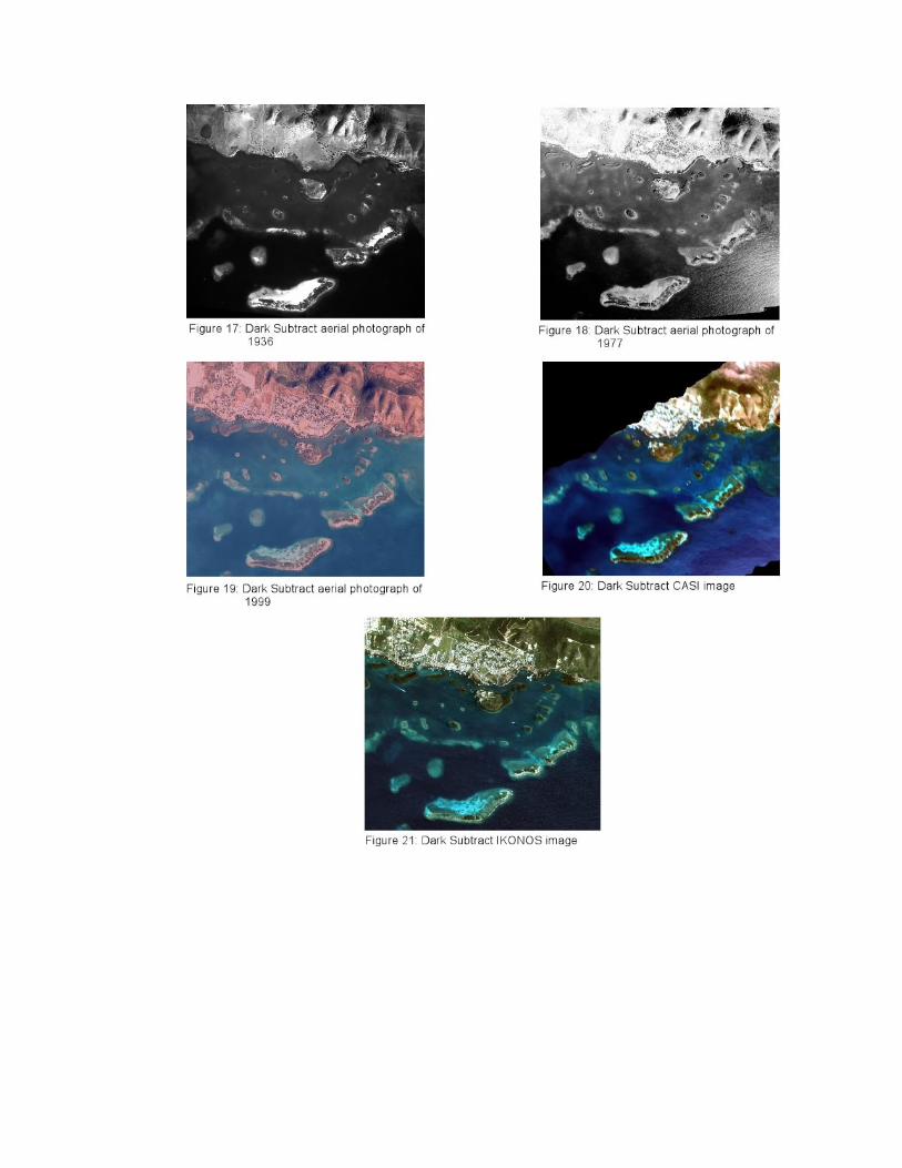
Results and Discussion I. Description for the aerial photographs and images
Dark subtract was used to remove the effect of the atmosphere that affects negatively the
outcome classification of the images and photos. Comparing these images and photos (figures:
17, 18, 19, 20 & 21) it is possible to see changes. The most noticeable change is found in the
main land. Urban development largely increased since 1936 until 1977, and from this year to
2001 (IKONOS image) such changes are less dramatic. There is no floating house in the coastal
line in 1936, but in 1977 until the present they are found. The second most noticeable change is
located in the coral reefs were the sand had been reduced and taken by the sea grass community.
In the coastline, just north of Magueyes Island there is a wetland area in 1936 that have been
reduced, specifically their water content. The amount of mangroves has increase in this area.
These wetlands have been covered with houses, buildings, and roads since 1977.
Mangroves in general are not well detected in 1936, mainly because of the quality of the
aerial photograph. This demonstrates the limitation of using black and white photos for this type
of work. Areas with sandy bottom in 1936 were covered by mangroves in 1977 and until
present.
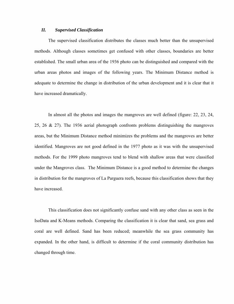
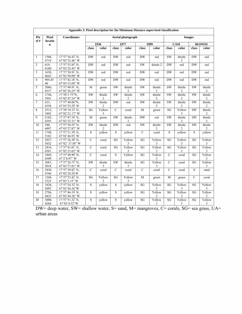
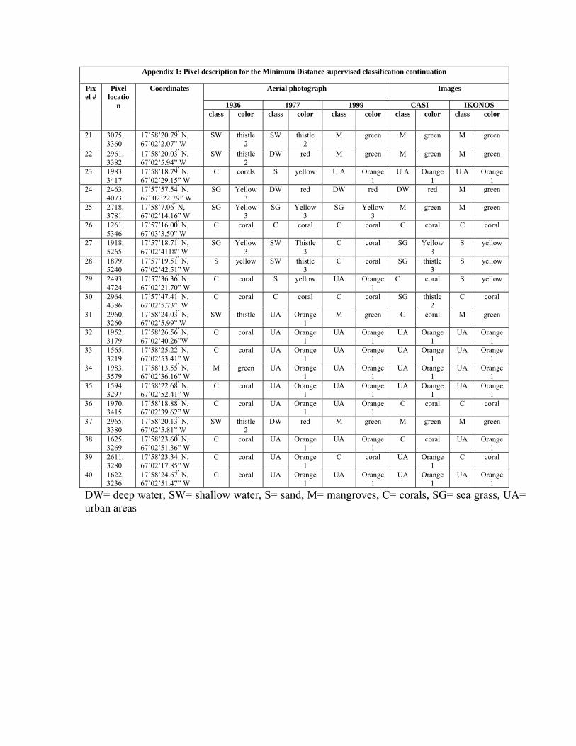
II. Supervised Classification
The supervised classification distributes the classes much better than the unsupervised
methods. Although classes sometimes get confused with other classes, boundaries are better
established. The small urban area of the 1936 photo can be distinguished and compared with the
urban areas photos and images of the following years. The Minimum Distance method is
adequate to determine the change in distribution of the urban development and it is clear that it
have increased dramatically.
In almost all the photos and images the mangroves are well defined (figure: 22, 23, 24,
25, 26 & 27). The 1936 aerial photograph confronts problems distinguishing the mangroves
areas, but the Minimum Distance method minimizes the problems and the mangroves are better
identified. Mangroves are not good defined in the 1977 photo as it was with the unsupervised
methods. For the 1999 photo mangroves tend to blend with shallow areas that were classified
under the Mangroves class. The Minimum Distance is a good method to determine the changes
in distribution for the mangroves of La Parguera reefs, because this classification shows that they
have increased.
This classification does not significantly confuse sand with any other class as seen in the
IsoData and K-Means methods. Comparing the classification it is clear that sand, sea grass and
coral are well defined. Sand has been reduced; meanwhile the sea grass community has
expanded. In the other hand, is difficult to determine if the coral community distribution has
changed through time.
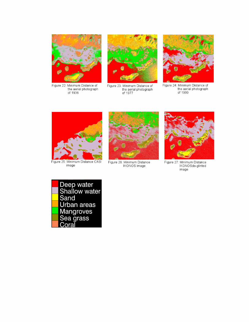
Table 2:Color interpretation for aerial photograph and images of Minimum Distance supervised classification
Class Color 1936 1977 1999 CASI IKONOS Deep water
Red Deep water Deep water, coral reefs, sea grass and mangroves
Deep water Deep water and sea grass
Deep water
Shallow water
Thistle 2 Shallow water, sea grass, coral reefs and mangroves
Shallow water, sea grass, coral reefs and mangroves
Shallow water
Shallow water
Shallow water and sea grass
Sand Yellow Sand and urban areas
Sand and coral reefs
Sand and coral reefs
Sand Sand
Sea grass
Yellow 3
Sea grass, coral reefs and shallow water
Sea grass, coral reefs and shallow water
Sea grass and shallow water
Sea grass and shallow water
Sea grass, coral reefs and shallow water
Mangroves
Green 1 Deep water and mangroves
Sea grass and mangroves
Shallow water, coral reefs and mangroves
Mangroves and coral reefs
Mangroves
Coral Coral Coral reefs, shallow water and sea grass
Coral reefs, shallow water and sea grass
Coral reefs, shallow water, mangroves and sea grass
Coral reefs, shallow water, mangroves and sea grass
Coral reefs and urban areas
Urban areas
Orange 1
Coral reef and sand
Urban areas and sand
Sea grass and shallow water
Urban areas Urban areas and sand
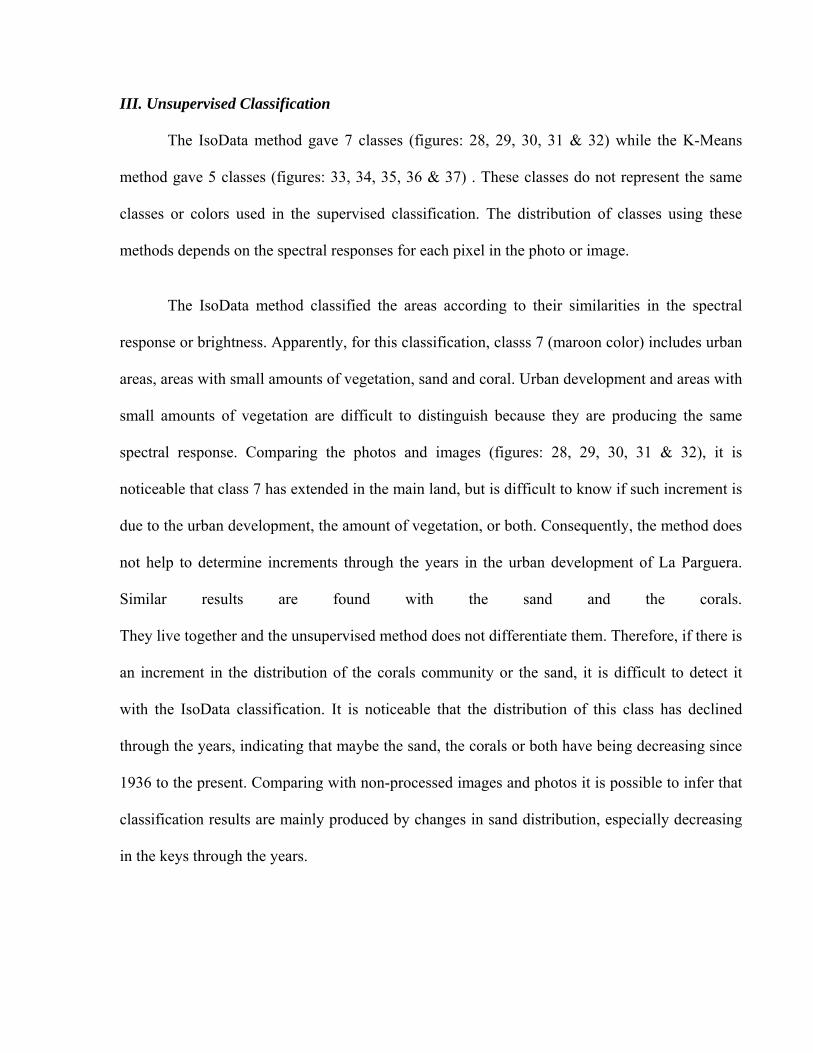
III. Unsupervised Classification
The IsoData method gave 7 classes (figures: 28, 29, 30, 31 & 32) while the K-Means
method gave 5 classes (figures: 33, 34, 35, 36 & 37) . These classes do not represent the same
classes or colors used in the supervised classification. The distribution of classes using these
methods depends on the spectral responses for each pixel in the photo or image.
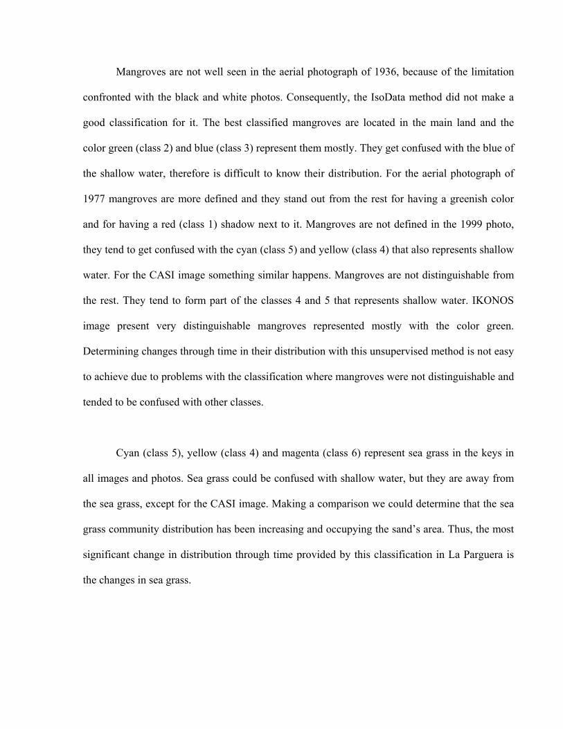
The IsoData method classified the areas according to their similarities in the spectral
response or brightness. Apparently, for this classification, classs 7 (maroon color) includes urban
areas, areas with small amounts of vegetation, sand and coral. Urban development and areas with
small amounts of vegetation are difficult to distinguish because they are producing the same
spectral response. Comparing the photos and images (figures: 28, 29, 30, 31 & 32), it is
noticeable that class 7 has extended in the main land, but is difficult to know if such increment is
due to the urban development, the amount of vegetation, or both. Consequently, the method does
not help to determine increments through the years in the urban development of La Parguera.
Similar results are found with the sand and the corals.
They live together and the unsupervised method does not differentiate them. Therefore, if there is
an increment in the distribution of the corals community or the sand, it is difficult to detect it
with the IsoData classification. It is noticeable that the distribution of this class has declined
through the years, indicating that maybe the sand, the corals or both have being decreasing since
1936 to the present. Comparing with non-processed images and photos it is possible to infer that
classification results are mainly produced by changes in sand distribution, especially decreasing
in the keys through the years.
Mangroves are not well seen in the aerial photograph of 1936, because of the limitation
confronted with the black and white photos. Consequently, the IsoData method did not make a
good classification for it. The best classified mangroves are located in the main land and the
color green (class 2) and blue (class 3) represent them mostly. They get confused with the blue of
the shallow water, therefore is difficult to know their distribution. For the aerial photograph of
1977 mangroves are more defined and they stand out from the rest for having a greenish color
and for having a red (class 1) shadow next to it. Mangroves are not defined in the 1999 photo,
they tend to get confused with the cyan (class 5) and yellow (class 4) that also represents shallow
water. For the CASI image something similar happens. Mangroves are not distinguishable from
the rest. They tend to form part of the classes 4 and 5 that represents shallow water. IKONOS
image present very distinguishable mangroves represented mostly with the color green.
Determining changes through time in their distribution with this unsupervised method is not easy
to achieve due to problems with the classification where mangroves were not distinguishable and
tended to be confused with other classes.
Cyan (class 5), yellow (class 4) and magenta (class 6) represent sea grass in the keys in
all images and photos. Sea grass could be confused with shallow water, but they are away from
the sea grass, except for the CASI image. Making a comparison we could determine that the sea
grass community distribution has been increasing and occupying the sand’s area. Thus, the most
significant change in distribution through time provided by this classification in La Parguera is
the changes in sea grass.
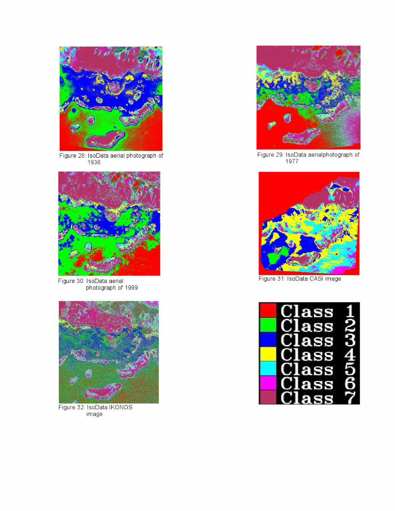

Table 3: Color interpretation for aerial photograph and images of IsoData classification Class Color 1936 1977 1999 CASI IKONOS
1 Red Deep water Deep water Deep water What is not part of the image
Mask
2 Green Deep water and mangroves
Deep water, sea grass and mangroves
Deep water Deep water and corals
Mangroves
3 Blue Shallow water and mangroves
Shallow water, mangroves and sea grass
Shallow water, sea grass and mangroves
Deep water, coral, sea grass and mangroves
Deep water and mangroves
4 Yellow Shallow water, submerged areas in coastal line and sea grass
Shallow water, sediment and sea grass
Shallow water, mangroves and sea grass
Shallow water, mangroves, coral and sea grass
Deep water, sea grass, and mangroves
5 Cyan Submerged areas in coastal line land, sea grass and shallow water
Sea grass and shallow water
shallow water sea, grass and mangroves
Shallow water, sea grass, coral and mangroves
Shallow water and sea grass
6 Magenta Submerged areas in coastal line, shallow water and sea grass
Shallow water, mangroves, coral and sea grass
Shallow water, mangroves. Coral and sea grass
Shallow water, sea grass and mangroves
Shallow water, coral and sea grass
7 Maroon Sand, coral, urban areas, submerged and little vegetation areas in main land
Sand, coral, urban areas and areas with little or without vegetation
Sand, coral, urban areas and areas with little or no vegetation
Sand and urban areas
Sand, urban areas, coral areas little or no vegetation
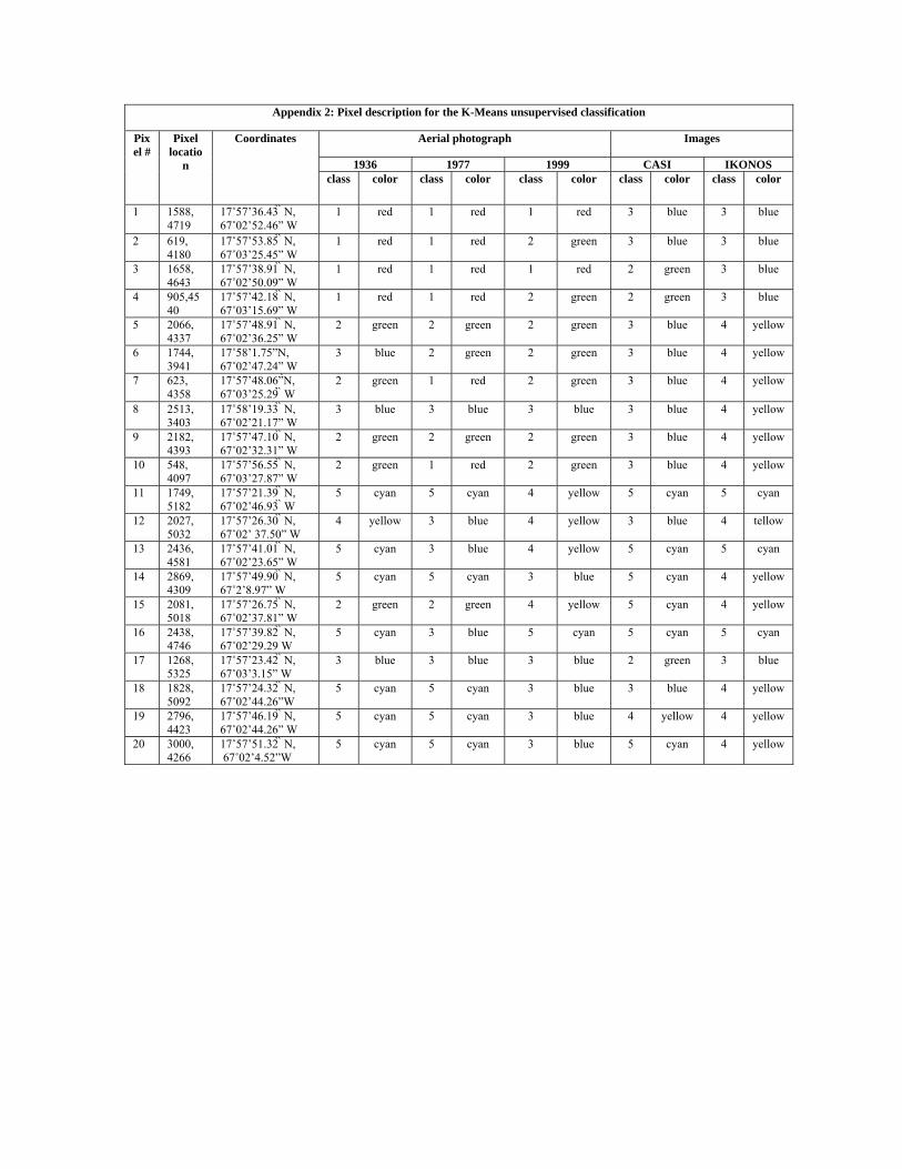
K-Means classification shows a pattern similar to the one found in the urban areas, in the
areas covered with sand and corals of the IsoData classification. It confuses the urban areas, the
sandy regions and the corals and gives them the same class (class 5, blue). It is not a good
method to determine increments in the urban areas. This must be, due to the quality (spatial
resolution) of the photos and images, because if all the photos and images had a high spatial
resolution the classification must had an outcome such as the one for the IKONOS image. In this
image the urban areas are well seen and distinguished.

Sand and corals are not differentiated and since they are next to the other is difficult to
determine which of them had changed their distribution through the years. There has been a
decrease in their distribution as the years have passed, but which of them had been reduced is not
determined with this method.
Mangroves were not well classified in the 1936 due to the same reason for which the
IsoData method did not classify it well. It is for the limitation of the black and white photos.
Only in the 1977 photo and the IKONOS image provide a clear distribution of the mangroves
represented by the class 2 (green), but if it has increased or decreased through the year can not be
determined, because of the lack of well classified photos or images of other years.
Sea grass are represented by the classes 4 (yellow) and 3 (blue) and its distribution change
can be determined because it does not get confused with any other mentioned above. The only
problem notable is the confusion presented in the CASI image where the sea grass blends with
shallow water represented by the class 1. According with this classification the sea grass
distribution has been increasing through the years. This method is adequate to determine changes
through years in the distribution of the sea grass of La Parguera reefs.


Table 4: Color interpretation for aerial photograph and images of K-Means classification Class Color 1936 1977 1999 CASI IKONOS
1 Red Deep water Deep water, mangroves and sea grass
Deep water What is not part of the photo
Mangroves and mask
2 Green Shallow water, sea grass and mangroves
Shallow water, sea grass and mangroves
Shallow water
Deep water, sea grass, coral reefs and mangroves
Mangroves
3 Blue Shallow water, sea grass, mangroves and submerged coastal line
Shallow water, sea grass and mangroves
Shallow water, sea grass and mangroves
Shallow water, sea grass, coral reefs and mangroves
Deep water, sea grass and mangroves
4 Yellow Submerged coastal line and shallow water
Shallow water, coral reefs sea grass and mangroves
Shallow water, coral reefs sea grass and mangroves
Shallow water, coral reefs, sea grass and mangroves
Shallow water, sea grass coral reefs and mangroves
5 Cyan Urban areas, sand, coral reefs, sea grass and submerged coastal line
Urban areas, coral reefs and sand
Urban areas, coral reefs and sand
Urban areas, coral reefs and sand
Urban areas, shallow water, coral reefs, areas with little or no vegetation and sand

Conclusion Changes in time in the distribution or spectral response of the ecosystems of La
Paraguera coral reefs can be dectected using Remote Sensing. These changes are detected using
the Minimum Distance unsupervised classification. From the three classification used, this one
detected more changes in distribution of the coral reefs of La Parguera. It detected urban areas
increment, expansion in the sea grass communities and mangroves, and sand reduction. Though
corals were distinguished, for this supervised method is difficult to detect changes through time
in their distribution. The IsoData and K-Means only detected expansion in the sea grass
communities. Therefore, none of these unsupervised methods are similar to the Minimum
Distance method.
The best sensor for this work was the IKONOS because of its high spatial resolution.
This make easier to differentiate from one class to the other. Camera sensor can also be used,
but details are lost due to its low spatial resolution. Black and white photos are not the best
option for this kind of work because of their limitation of color that confuses and loses
information. CASI is not the best sensor from them all, because frequently, due to its low spatial
resolution, details of the area were hard to see.
Although, processing the images with the classifications already mentioned, can detect
changes through time in the distribution in La Pargueras coral reefs, the truth is that these
changes are easily detected without the processing. Thus, classifying the images can help to
determine the changes, but these changes can be detected comparing the original aerial
photographs and images.

Bibligraphy: Andrefouet, S., Broca, J., Garza, R., Hatcher, B., Hochberg, E., Joyce, K., Kramer, P.,
Muller, F., Mumby, P., Nasser, A., Phinn, S., Reigl, B., Torres, D., White, W., Yamano, H., Zubia, M. 2002. Multi-site evaluation of IKONOS data for classification of tropical coral Reef environments. Remote Sensing of Environment. pp 1-14.
Bruckner, A., Carlo, M., Morelock, J. and Ramírez, W. 2001. Status of Coral Reefs, Southwest Puerto Rico. University of Puerto Rico, Mayagüez Campus (UPRM) website. http://www.uprm.edu/biology/cjs/reefstatus.htm.
Center of Imaging Science (CIS) .2004. Atmospheric correction. CIS website. http://www.cis.rit.edu/research/dirs/research/atmos_corr.html Coral Reef Information System (CoRIS). 2004. About Coral Reefs- Hazards to coral reefs.
CoRIS website. http://www.coris.noaa.gov/about/hazards/hazards.html. CNN Earth story page. 1997. Earth's coral reefs in decline, researchers say. CNN website. http://www.cnn.com/EARTH/9712/30/year.of.reef/. Decision Support. 2003.Georefencing. Columbus website. http://www.dsigeotim.net/imageprocessing.html Gilbes, F. 2004. Image Classification. http://cacique.uprm.edu/geol4048/classification.pdf. Campbell, J. 2002. Introduction to Remote Sensing. Third Edition. New York. The Gilford Press. ITRES. 2003. When was CASI first developed? ITRES website. http://www.itres.com/docs/faq.html. Ocean World. 2004.Coral reefs destruction and conservation. Ocean World website. http://oceanworld.tamu.edu/students/coral/coral5.htm Space Imaging. 2004. IKONOS sensor overview. Space Imaging website.
http://www.spaceimaging.com/products/ikonos/index_2.htm. Space Images News Release. 2000. NOAA using commercial satellite to study coral reefs. Space Flight Now website. http://spaceflightnow.com/news/n0011/20ikonosnoaa/.

Appendix
Appendix 1: Pixel description for the IsoData unsupervised classification
Aerial photograph Images
1936 1977 1999 CASI IKONOS
Pixel #
Pixel locatio
n
Coordinates
class color class color class color class color class color
1
1588, 4719
17˚57’36.43̀ ̀ N, 67˚02’52.46” W
2 green 1 red 2 green 3 blue 4 yellow
2 619, 4180
17˚57’53.85̀ ̀ N, 67˚03’25.45” W
1 red 1 red 2 green 3 blue 4 yellow
3 1658, 4643
17˚57’38.91̀ ̀ N, 67˚02’50.09” W
2 green 1 red 2 green 3 blue 4 yellow
4 905,4540
17˚57’42.18̀ ̀ N, 67˚03’15.69” W
2 green 1 red 2 green 3 blue 4 yellow
5 2066, 4337
17˚57’48.91̀ ̀ N, 67˚02’36.25” W
2 green 3 green 2 green 5 cyan 5 cyan
6 1744, 3941
17˚58’1.75”N, 67˚02’47.24” W
3 blue 2 green 3 blue 5 cyan 3 blue
7 623, 4358
17˚57’48.06” ̀N, 67˚03’25.29̀̀ ̀ W
3 blue 1 red 3 blue 4 yellow 3 blue
8 2513, 3403
17˚58’19.33̀ ̀ N, 67˚02’21.17” W
4 yellow 5 cyan 4 yellow 5 cyan 5 cyan
9 2182, 4393
17˚57’47.10̀ ̀ N, 67˚02’32.31” W
3 blue 2 green 2 green 5 cyan 4 yellow
10 548, 4097
17˚57’56.55̀ ̀ N, 67˚03’27.87” W
3 blue 1 red 2 green 4 yellow 5 Cyan
11 1749, 5182
17˚57’21.39̀ ̀ N, 67˚02’46.93̀ ̀ W
7 maroon 7 maroon 6 magenta
7 maroon 7 maroon
12 2027, 5032
17˚57’26.30̀ ̀ N, 67˚02’ 37.50” W
5 cyan 4 yellow 5 cyan 4 yellow 6 magenta
13 2436, 4581
17˚57’41.01̀ ̀ N, 67˚02’23.65” W
7 maroon 4 yellow 5 cyan 6 magenta
7 maroon
14 2869, 4309
17˚57’49.90̀ ̀ N, 67˚2’8.97” W
7 maroon 7 maroon 4 yellow 7 maroon 6 magenta
15 2081, 5018
17˚57’26.75̀ ̀ N, 67˚02’37.81” W
7 maroon 5 cyan 5 cyan 4 yellow 5 cyan
16 2438, 4746
17˚57’39.82̀ ̀ N, 67˚02’29.29 W
4 yellow 6 magenta
5 cyan 5 cyan 5 cyan
17 1268, 5325
17˚57’23.42̀ ̀ N, 67˚03’3.15” W
7 maroon 7 maroon 7 maroon 7 maroon 7 maroon
18 1828, 5092
17˚57’24.32̀ ̀ N, 67˚02’44.26”W
7 maroon 7 maroon 5 cyan 5 cyan 6 magenta
19 2796, 4423
17˚57’46.19̀ ̀ N, 67˚02’44.26” W
7 maroon 7 maroon 4 yellow 6 magenta
5 cyan
20 3000, 4266
17˚57’51.32̀ ̀ N, 67˚02’4.52”W
7 maroon 7 maroon 4 yellow 7 maroon 6 magenta
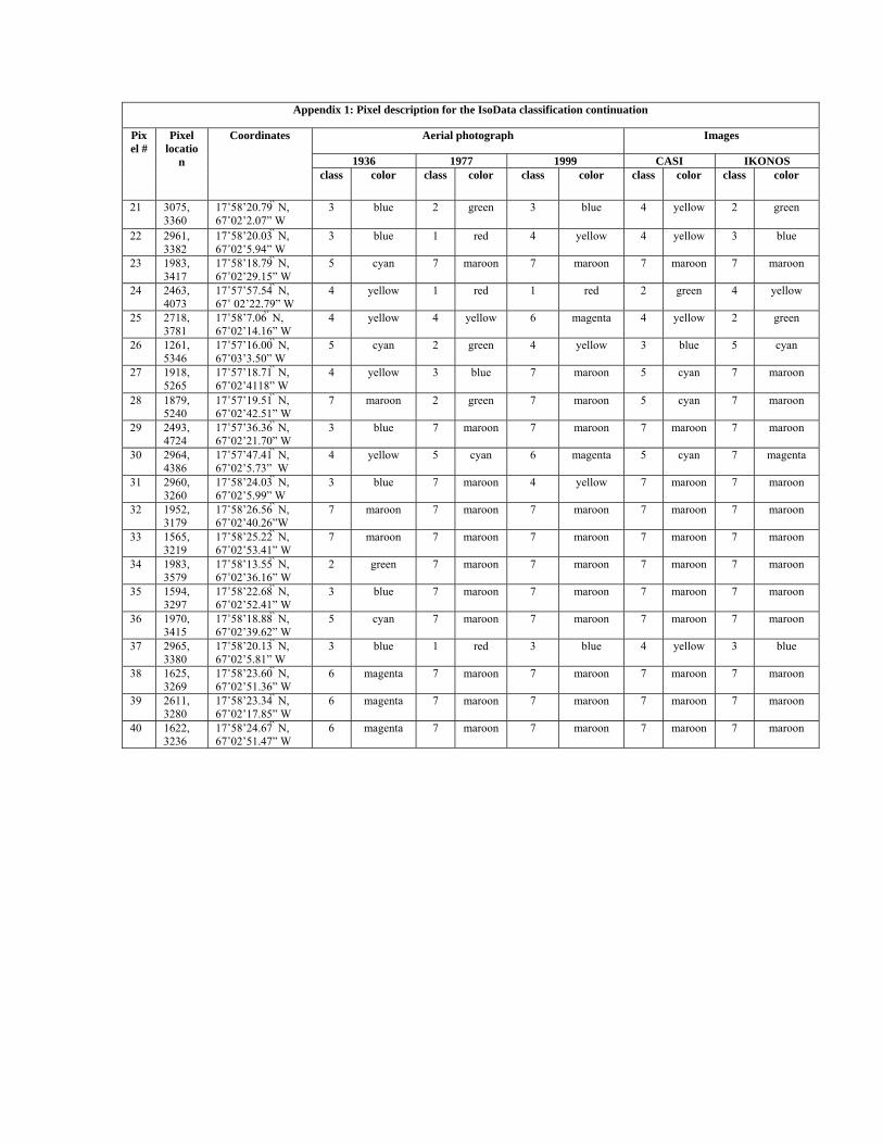
Appendix 1: Pixel description for the IsoData classification continuation
Aerial photograph Images
1936 1977 1999 CASI IKONOS
Pixel #
Pixel locatio
n
Coordinates
class color class color class color class color class color
21 3075, 3360
17˚58’20.79̀ ̀ N, 67˚02’2.07” W
3 blue 2 green 3 blue 4 yellow 2 green
22 2961, 3382
17˚58’20.03̀ ̀ N, 67˚02’5.94” W
3 blue 1 red 4 yellow 4 yellow 3 blue
23 1983, 3417
17˚58’18.79̀ ̀ N, 67˚02’29.15” W
5 cyan 7 maroon 7 maroon 7 maroon 7 maroon
24 2463, 4073
17˚57’57.54̀ ̀ N, 67˚ 02’22.79” W
4 yellow 1 red 1 red 2 green 4 yellow
25 2718, 3781
17˚58’7.06̀ ̀ N, 67˚02’14.16” W
4 yellow 4 yellow 6 magenta 4 yellow 2 green
26 1261, 5346
17˚57’16.00̀ ̀ N, 67˚03’3.50” W
5 cyan 2 green 4 yellow 3 blue 5 cyan
27 1918, 5265
17˚57’18.71̀ ̀ N, 67˚02’4118” W
4 yellow 3 blue 7 maroon 5 cyan 7 maroon
28 1879, 5240
17˚57’19.51̀ ̀ N, 67˚02’42.51” W
7 maroon 2 green 7 maroon 5 cyan 7 maroon
29 2493, 4724
17˚57’36.36̀ ̀ N, 67˚02’21.70” W
3 blue 7 maroon 7 maroon 7 maroon 7 maroon
30 2964, 4386
17˚57’47.41̀ ̀ N, 67˚02’5.73” W
4 yellow 5 cyan 6 magenta 5 cyan 7 magenta
31 2960, 3260
17˚58’24.03̀ ̀ N, 67˚02’5.99” W
3 blue 7 maroon 4 yellow 7 maroon 7 maroon
32 1952, 3179
17˚58’26.56̀ ̀ N, 67˚02’40.26”W
7 maroon 7 maroon 7 maroon 7 maroon 7 maroon
33 1565, 3219
17˚58’25.22̀ ̀ N, 67˚02’53.41” W
7 maroon 7 maroon 7 maroon 7 maroon 7 maroon
34 1983, 3579
17˚58’13.55̀ ̀ N, 67˚02’36.16” W
2 green 7 maroon 7 maroon 7 maroon 7 maroon
35 1594, 3297
17˚58’22.68̀ ̀ N, 67˚02’52.41” W
3 blue 7 maroon 7 maroon 7 maroon 7 maroon
36 1970, 3415
17˚58’18.88̀ ̀ N, 67˚02’39.62” W
5 cyan 7 maroon 7 maroon 7 maroon 7 maroon
37 2965, 3380
17˚58’20.13̀ ̀ N, 67˚02’5.81” W
3 blue 1 red 3 blue 4 yellow 3 blue
38 1625, 3269
17˚58’23.60̀ ̀ N, 67˚02’51.36” W
6 magenta 7 maroon 7 maroon 7 maroon 7 maroon
39 2611, 3280
17˚58’23.34̀ ̀ N, 67˚02’17.85” W
6 magenta 7 maroon 7 maroon 7 maroon 7 maroon
40 1622, 3236
17˚58’24.67̀ ̀ N, 67˚02’51.47” W
6 magenta 7 maroon 7 maroon 7 maroon 7 maroon
Appendix 2: Pixel description for the K-Means unsupervised classification
Aerial photograph Images
1936 1977 1999 CASI IKONOS
Pixel #
Pixel locatio
n
Coordinates
class color class color class color class color class color
1
1588, 4719
17˚57’36.43̀ ̀ N, 67˚02’52.46” W
1 red 1 red 1 red 3 blue 3 blue
2 619, 4180
17˚57’53.85̀ ̀ N, 67˚03’25.45” W
1 red 1 red 2 green 3 blue 3 blue
3 1658, 4643
17˚57’38.91̀ ̀ N, 67˚02’50.09” W
1 red 1 red 1 red 2 green 3 blue
4 905,4540
17˚57’42.18̀ ̀ N, 67˚03’15.69” W
1 red 1 red 2 green 2 green 3 blue
5 2066, 4337
17˚57’48.91̀ ̀ N, 67˚02’36.25” W
2 green 2 green 2 green 3 blue 4 yellow
6 1744, 3941
17˚58’1.75”N, 67˚02’47.24” W
3 blue 2 green 2 green 3 blue 4 yellow
7 623, 4358
17˚57’48.06” ̀N, 67˚03’25.29̀̀ ̀ W
2 green 1 red 2 green 3 blue 4 yellow
8 2513, 3403
17˚58’19.33̀ ̀ N, 67˚02’21.17” W
3 blue 3 blue 3 blue 3 blue 4 yellow
9 2182, 4393
17˚57’47.10̀ ̀ N, 67˚02’32.31” W
2 green 2 green 2 green 3 blue 4 yellow
10 548, 4097
17˚57’56.55̀ ̀ N, 67˚03’27.87” W
2 green 1 red 2 green 3 blue 4 yellow
11 1749, 5182
17˚57’21.39̀ ̀ N, 67˚02’46.93̀ ̀ W
5 cyan 5 cyan 4 yellow 5 cyan 5 cyan
12 2027, 5032
17˚57’26.30̀ ̀ N, 67˚02’ 37.50” W
4 yellow 3 blue 4 yellow 3 blue 4 tellow
13 2436, 4581
17˚57’41.01̀ ̀ N, 67˚02’23.65” W
5 cyan 3 blue 4 yellow 5 cyan 5 cyan
14 2869, 4309
17˚57’49.90̀ ̀ N, 67˚2’8.97” W
5 cyan 5 cyan 3 blue 5 cyan 4 yellow
15 2081, 5018
17˚57’26.75̀ ̀ N, 67˚02’37.81” W
2 green 2 green 4 yellow 5 cyan 4 yellow
16 2438, 4746
17˚57’39.82̀ ̀ N, 67˚02’29.29 W
5 cyan 3 blue 5 cyan 5 cyan 5 cyan
17 1268, 5325
17˚57’23.42̀ ̀ N, 67˚03’3.15” W
3 blue 3 blue 3 blue 2 green 3 blue
18 1828, 5092
17˚57’24.32̀ ̀ N, 67˚02’44.26”W
5 cyan 5 cyan 3 blue 3 blue 4 yellow
19 2796, 4423
17˚57’46.19̀ ̀ N, 67˚02’44.26” W
5 cyan 5 cyan 3 blue 4 yellow 4 yellow
20 3000, 4266
17˚57’51.32̀ ̀ N, 67˚02’4.52”W
5 cyan 5 cyan 3 blue 5 cyan 4 yellow

Appendix 2: Pixel description for the K-Means classification continuation
Aerial photograph Images
1936 1977 1999 CASI IKONOS
Pixel #
Pixel locatio
n
Coordinates
class color class color class color class color class color
21 3075, 3360
17˚58’20.79̀ ̀ N, 67˚02’2.07” W
2 green 2 green 3 blue 3 blue 2 green
22 2961, 3382
17˚58’20.03̀ ̀ N, 67˚02’5.94” W
3 blue 4 yellow 3 blue 4 yellow 3 blue
23 1983, 3417
17˚58’18.79̀ ̀ N, 67˚02’29.15” W
4 yellow 5 cyan 5 cyan 5 cyan 5 cyan
24 2463, 4073
17˚57’57.54̀ ̀ N, 67˚ 02’22.79” W
4 yellow 5 cyan 5 cyan 5 cyan 5 cyan
25 2718, 3781
17˚58’7.06̀ ̀ N, 67˚02’14.16” W
3 blue 3 blue 4 yellow 3 blue 2 green
26 1261, 5346
17˚57’16.00̀ ̀ N, 67˚03’3.50” W
4 yellow 5 cyan 5 cyan 5 cyan 5 cyan
27 1918, 5265
17˚57’18.71̀ ̀ N, 67˚02’4118” W
3 blue 2 green 5 cyan 4 yellow 5 cyan
28 1879, 5240
17˚57’19.51̀ ̀ N, 67˚02’42.51” W
1 red 1 red 1 red 2 green 3 blue
29 2493, 4724
17˚57’36.36̀ ̀ N, 67˚02’21.70” W
3 blue 5 cyan 5 cyan 5 cyan 5 cyan
30 2964, 4386
17˚57’47.41̀ ̀ N, 67˚02’5.73” W
3 blue 4 yellow 5 cyan 3 blue 5 cyan
31 2960, 3260
17˚58’24.03̀ ̀ N, 67˚02’5.99” W
3 blue 5 cyan 3 blue 5 cyan 5 cyan
32 1952, 3179
17˚58’26.56̀ ̀ N, 67˚02’40.26”W
5 cyan 5 cyan 5 cyan 5 cyan 5 cyan
33 1565, 3219
17˚58’25.22̀ ̀ N, 67˚02’53.41” W
5 cyan 5 cyan 5 cyan 5 cyan 5 cyan
34 1983, 3579
17˚58’13.55̀ ̀ N, 67˚02’36.16” W
3 blue 4 yellow 5 cyan 5 cyan 5 cyan
35 1594, 3297
17˚58’22.68̀ ̀ N, 67˚02’52.41” W
2 green 5 cyan 5 cyan 5 cyan 5 cyan
36 1970, 3415
17˚58’18.88̀ ̀ N, 67˚02’39.62” W
3 blue 5 cyan 5 cyan 5 cyan 5 cyan
37 2965, 3380
17˚58’20.13̀ ̀ N, 67˚02’5.81” W
3 blue 1 red 3 blue 3 blue 2 green
38 1625, 3269
17˚58’23.60̀ ̀ N, 67˚02’51.36” W
4 yellow 5 cyan 5 cyan 5 cyan 5 cyan
39 2611, 3280
17˚58’23.34̀ ̀ N, 67˚02’17.85” W
4 yellow 5 cyan 5 cyan 5 cyan 5 cyan
40 1622, 3236
17˚58’24.67̀ ̀ N, 67˚02’51.47” W
4 yellow 5 cyan 5 cyan 5 cyan 5 cyan
Appendix 3: Pixel description for the Minimum Distance supervised classification
Aerial photograph Images
1936 1977 1999 CASI IKONOS
Pixel #
Pixel locatio
n
Coordinates
class color class color class color class color class color
1
1588, 4719
17˚57’36.43̀ ̀ N, 67˚02’52.46” W
DW red DW red DW red SW thistle 2
DW red
2 619, 4180
17˚57’53.85̀ ̀ N, 67˚03’25.45” W
DW red DW red SW thistle 2 DW red DW red
3 1658, 4643
17˚57’38.91̀ ̀ N, 67˚02’50.09” W
DW red DW red DW red DW red DW red
4 905,4540
17˚57’42.18̀ ̀ N, 67˚03’15.69” W
DW red DW red DW red DW red DW red
5 2066, 4337
17˚57’48.91̀ ̀ N, 67˚02’36.25” W
M green SW thistle 2
SW thistle 2
SW thistle 2
SW thistle 2
6 1744, 3941
17˚58’1.75”N, 67˚02’47.24” W
SW thistle 2
SW thistle 2
SW thistle 2
SW thistle 2
SW thistle 2
7 623, 4358
17˚57’48.06” ̀N, 67˚03’25.29̀̀ ̀ W
SW thistle 2
DW red SW thistle 2
SW thistle 2
SW thistle 2
8 2513, 3403
17˚58’19.33̀ ̀ N, 67˚02’21.17” W
SG Yellow 3
C coral M green SG Yellow3
SW thistle 2
9 2182, 4393
17˚57’47.10̀ ̀ N, 67˚02’32.31” W
M green SW thistle 2
DW red SW thistle 2
SW thistle 2
10 548, 4097
17˚57’56.55̀ ̀ N, 67˚03’27.87” W
SW thistle 2
DW red SW thistle 2
SW thistle 2
SW thistle 2
11 1749, 5182
17˚57’21.39̀ ̀ N, 67˚02’46.93̀ ̀ W
S yellow S yellow C coral S yellow S yellow
12 2027, 5032
17˚57’26.30̀ ̀ N, 67˚02’ 37.50” W
C coral SG Yellow 3
SG Yellow 3
SG Yellow 3
SG Yellow 3
13 2436, 4581
17˚57’41.01̀ ̀ N, 67˚02’23.65” W
C coral SG Yellow 3
SG Yellow 3
SG Yellow 3
SG Yellow 3
14 2869, 4309
17˚57’49.90̀ ̀ N, 67˚2’8.97” W
C coral S Yellow SG Yellow 3
C coral SG Yellow 3
15 2081, 5018
17˚57’26.75̀ ̀ N, 67˚02’37.81” W
SW thistle 3
SW thistle 3
SG Yellow 3
C coral SG Yellow 3
16 2438, 4746
17˚57’39.82̀ ̀ N, 67˚02’29.29 W
C coral C coral C coral C coral S sand
17 1268, 5325
17˚57’23.42̀ ̀ N, 67˚03’3.15” W
SG Yellow 3
SG Yellow 3
M green M green C coral
18 1828, 5092
17˚57’24.32̀ ̀ N, 67˚02’44.26”W
S yellow S yellow SG Yellow 3
SG Yellow 3
SG Yellow 3
19 2796, 4423
17˚57’46.19̀ ̀ N, 67˚02’44.26” W
S yellow S yellow SG Yellow 3
SG Yellow 3
SG Yellow 3
20 3000, 4266
17˚57’51.32̀ ̀ N, 67˚02’4.52”W
S yellow S yellow SG Yellow 3
SG Yellow 3
SG Yellow 3
DW= deep water, SW= shallow water, S= sand, M= mangroves, C= corals, SG= sea grass, UA= urban areas
Appendix 1: Pixel description for the Minimum Distance supervised classification continuation
Aerial photograph Images
1936 1977 1999 CASI IKONOS
Pixel #
Pixel locatio
n
Coordinates
class color class color class color class color class color
21 3075, 3360
17˚58’20.79̀ ̀ N, 67˚02’2.07” W
SW thistle 2
SW thistle 2
M green M green M green
22 2961, 3382
17˚58’20.03̀ ̀ N, 67˚02’5.94” W
SW thistle 2
DW red M green M green M green
23 1983, 3417
17˚58’18.79̀ ̀ N, 67˚02’29.15” W
C corals S yellow U A Orange 1
U A Orange 1
U A Orange 1
24 2463, 4073
17˚57’57.54̀ ̀ N, 67˚ 02’22.79” W
SG Yellow 3
DW red DW red DW red M green
25 2718, 3781
17˚58’7.06̀ ̀ N, 67˚02’14.16” W
SG Yellow 3
SG Yellow 3
SG Yellow 3
M green M green
26 1261, 5346
17˚57’16.00̀ ̀ N, 67˚03’3.50” W
C coral C coral C coral C coral C coral
27 1918, 5265
17˚57’18.71̀ ̀ N, 67˚02’4118” W
SG Yellow 3
SW Thistle 3
C coral SG Yellow 3
S yellow
28 1879, 5240
17˚57’19.51̀ ̀ N, 67˚02’42.51” W
S yellow SW thistle 3
C coral SG thistle 3
S yellow
29 2493, 4724
17˚57’36.36̀ ̀ N, 67˚02’21.70” W
C coral S yellow UA Orange 1
C coral S yellow
30 2964, 4386
17˚57’47.41̀ ̀ N, 67˚02’5.73” W
C coral C coral C coral SG thistle 2
C coral
31 2960, 3260
17˚58’24.03̀ ̀ N, 67˚02’5.99” W
SW thistle UA Orange 1
M green C coral M green
32 1952, 3179
17˚58’26.56̀ ̀ N, 67˚02’40.26”W
C coral UA Orange 1
UA Orange 1
UA Orange 1
UA Orange 1
33 1565, 3219
17˚58’25.22̀ ̀ N, 67˚02’53.41” W
C coral UA Orange 1
UA Orange 1
UA Orange 1
UA Orange 1
34 1983, 3579
17˚58’13.55̀ ̀ N, 67˚02’36.16” W
M green UA Orange 1
UA Orange 1
UA Orange 1
UA Orange 1
35 1594, 3297
17˚58’22.68̀ ̀ N, 67˚02’52.41” W
C coral UA Orange 1
UA Orange 1
UA Orange 1
UA Orange 1
36 1970, 3415
17˚58’18.88̀ ̀ N, 67˚02’39.62” W
C coral UA Orange 1
UA Orange 1
C coral C coral
37 2965, 3380
17˚58’20.13̀ ̀ N, 67˚02’5.81” W
SW thistle 2
DW red M green M green M green
38 1625, 3269
17˚58’23.60̀ ̀ N, 67˚02’51.36” W
C coral UA Orange 1
UA Orange 1
C coral UA Orange 1
39 2611, 3280
17˚58’23.34̀ ̀ N, 67˚02’17.85” W
C coral UA Orange 1
C coral UA Orange 1
C coral
40 1622, 3236
17˚58’24.67̀ ̀ N, 67˚02’51.47” W
C coral UA Orange 1
UA Orange 1
UA Orange 1
UA Orange 1
DW= deep water, SW= shallow water, S= sand, M= mangroves, C= corals, SG= sea grass, UA= urban areas


