Finding Mr. Schumpeter: An Empirical Study of Competition and Technology Adoption * Jeffrey Macher † Georgetown University Nathan H. Miller ‡ Georgetown University Matthew Osborne § University of Toronto February 27, 2017 Abstract We estimate the effect of competition on the adoption of a cost-reducing technology in the cement industry, using data that span 1953-2013. The new technology, the precalciner kiln, reduces fuel usage and hence fuel costs. We find adoption is more likely if the fuel cost savings are large, and less likely if there are many nearby competitors. We also find that competition damps the positive effect of cost savings. The results are consistent with a dynamic theoretical model in which competition can deprive firms of the scale necessary to recoup sunk adoption costs. Keywords: technology, innovation, competition, portland cement JEL classification: L1, L5, L6 * We thank Philippe Aghion, Jacob Cosman, Alberto Galasso, Richard Gilbert, Arik Levinsohn, Devesh Raval, John Rust, Rich Sweeney, Mihkel Tombak, Francis Vella, and seminar participants at Georgetown University, Harvard Business School, Harvard University, and the University of Toronto for helpful comments. We have benefited from conversations with Hendrick van Oss of the USGS and other industry participants. Conor Ryan provided research assistance. † Georgetown University, McDonough School of Business, 37th and O Streets NW, Washington DC 20057. Email: jeff[email protected]. ‡ Georgetown University, McDonough School of Business, 37th and O Streets NW, Washington DC 20057. Email: [email protected]. § University of Toronto, Rotman School of Management, 105 St. George Street, Toronto, ON, Canada M5S 3E6. Email: [email protected].
Transcript
Finding Mr. Schumpeter: An Empirical Study ofCompetition and Technology Adoption∗
Jeffrey Macher†
Georgetown UniversityNathan H. Miller‡
Georgetown University
Matthew Osborne§
University of Toronto
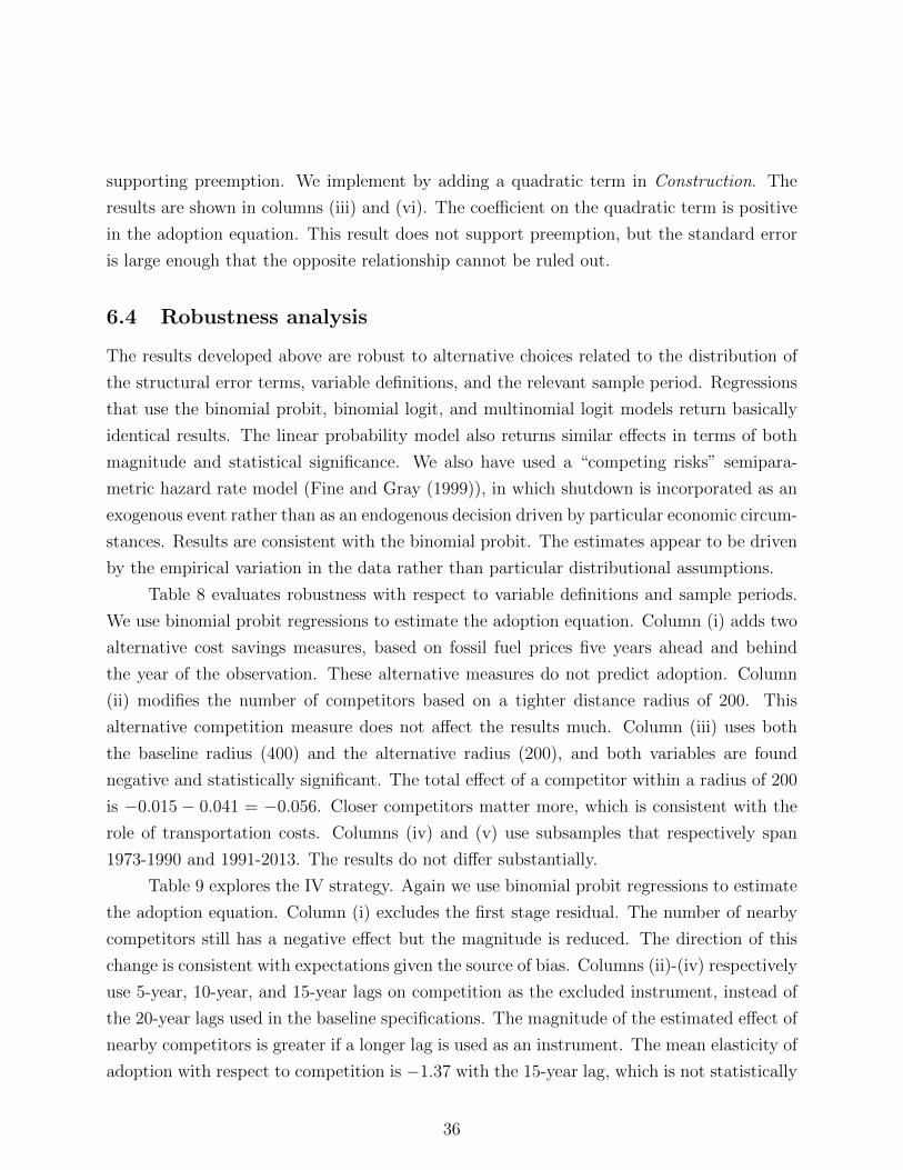
February 27, 2017
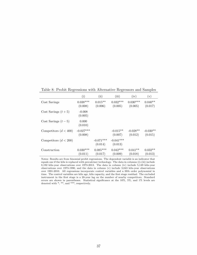
Abstract
We estimate the effect of competition on the adoption of a cost-reducing technologyin the cement industry, using data that span 1953-2013. The new technology, theprecalciner kiln, reduces fuel usage and hence fuel costs. We find adoption is more likelyif the fuel cost savings are large, and less likely if there are many nearby competitors.We also find that competition damps the positive effect of cost savings. The results areconsistent with a dynamic theoretical model in which competition can deprive firms ofthe scale necessary to recoup sunk adoption costs.
∗We thank Philippe Aghion, Jacob Cosman, Alberto Galasso, Richard Gilbert, Arik Levinsohn, DeveshRaval, John Rust, Rich Sweeney, Mihkel Tombak, Francis Vella, and seminar participants at GeorgetownUniversity, Harvard Business School, Harvard University, and the University of Toronto for helpful comments.We have benefited from conversations with Hendrick van Oss of the USGS and other industry participants.Conor Ryan provided research assistance.†Georgetown University, McDonough School of Business, 37th and O Streets NW, Washington DC 20057.
Email: [email protected].‡Georgetown University, McDonough School of Business, 37th and O Streets NW, Washington DC 20057.
Email: [email protected].§University of Toronto, Rotman School of Management, 105 St. George Street, Toronto, ON, Canada
Joseph Schumpeter (1934, 1942) famously argues that large firms in concentrated markets
invest more intensely in innovation. Empirical research on this hypothesis is challenging
because innovation is difficult to measure and because the explanatory variables—market
concentration and firm size—are endogenous economic outcomes. Further, the substantial
reduced-form literature often relies on cross-industry comparisons that are difficult to inter-
pret because the theoretical mechanisms that dominate in one industry may be unimportant
in others.1 Interest in the subject remains strong, however, and recent research makes
progress by using dynamic structural models to simulate the effect of competition in specific
settings (e.g., Goettler and Gordon (2011); Igami (2015); Igami and Uetake (2016)).
We contribute to this literature with a study of technology adoption in the portland
cement industry. We first develop a dynamic model of technology adoption to understand
the economic mechanisms at play. We then estimate the determinants of adoption with-
out imposing (much) structure on the model, which allows us to reach conclusions about
technology adoption that rely on the underlying empirical variation to the greatest extent
possible. This approach is made possible by the data at our disposal, which span the period
1953-2013 and include hundreds of older kilns that could be replaced with fuel efficient pre-
calciner kilns. The first precalciner kiln is installed in 1974, and precalciner kilns account
for 74 percent of industry capacity by the end of the sample. Most older kilns that are not
replaced are shut down instead. The analysis makes use of time-series variation in fossil fuel
prices, as well as time-series and cross-sectional variation in competition and demand.
The theoretical objective of the paper is to understand adoption for a particular class
of cost-reducing technologies. This class includes technologies for which adoption is (i) non-
drastic because equilibrium prices remain above the marginal cost of old technology; (ii)
non-divisible because adoption costs do not scale with capacity; and (iii) non-exclusive be-
cause adoption by one firm does not preclude others from adopting. This technology class
is most common in process-intensive industries (e.g., Abernathy and Utterback (1978)), and
arguably captures the most salient characteristics of precalciner adoption. We analyze a
simplified version of the dynamic oligopoly models that are used in theoretical and compu-
tational research to understand investment, entry, and exit decisions under uncertainty (e.g.,
Ericson and Pakes (1995); Doraszelski and Satterthwaite (2010)). We show that competi-
1Aghion and Tirole (1994) refer to the Schumpeterian hypothesis as the second most tested relationshipin industrial organization, following only the price-concentration relationship. Even the literature reviewsare daunting (e.g., Kamien and Schwartz (1982); Baldwin and Scott (1987); Cohen and Levin (1989); Cohen(1995); Gilbert (2006); Cohen (2010)).
1
tion limits long run adoption at least weakly. The mechanism is simple: competition denies
firms the scale necessary to recoup adoption costs. The presence of many competitors does
create preemption incentives and, in some parameterizations, competition speeds short-term
adoption even as it limits long run adoption.
The empirical analysis centers on multinomial probit regressions that characterize kiln
adoption and shutdown. The regressions can be interpreted as implementing the first step
in the standard two-step estimator for dynamic games (e.g., Bajari, Benkard and Levin
(2007); Ryan (2012)). We focus exclusively on the first step because we seek to understand
firm policies rather than conduct counterfactual simulations. The institutional details of the
industry—market power is localized due to high transportation costs—allow us to measure
competition based on the number of nearby competing plants. The main challenge for iden-
tification is that this competition measure could be positively correlated with the unobserved
error term, such that estimation risks understating the extent to which competition deters
adoption. We proceed using the control function approach of Rivers and Vuong (1988).
The excluded instrument is a 20-year lag on the competition variable. This lag has power
because kilns are long-lived, and it is valid provided that autocorrelation in the unobserved
error terms is not too great. We find that using a 15-year lag instead produces similar results,
which supports that the persistence of the error term dies out over longer time horizons.
The regression results indicate that plants facing greater competition are less likely
to adopt precalciner technology and more likely to shutter their older kilns. These effects
are statistically significant and robust across a number of alternative modeling assumptions.
The mean elasticity of the adoption probability with respect to competition ranges between
−1.45 and −2.16 in the baseline specifications. Interpreted through the lens of the theoretical
model, the empirical analysis supports that Schumpeterian scale effects dominate preemption
effects in the data. Supplementary checks do not find evidence of strong preemption effects:
for example, whether a plant is nearby early adopters has little additional explanatory power
on precalciner adoption and kiln shutdown. The other comparative statics of the theoretical
model find robust support in the data: the regressions indicate that adoption increases
with the fuel costs savings provided by precalciners (which depend on fossil fuel prices), the
amount of nearby construction activity, and the average fuel costs of nearby competitors.
These results reinforce the connections between the model and the data.
Our research has bearing on whether carbon taxes induce firms to adopt green technol-
ogy. Recent empirical articles on the so-called “induced innovation” hypothesis typically find
some margin of adjustment but do not address competition (e.g., Newell, Jaffe and Stavins
(1999); Popp (2002); Linn (2008); Aghion et al (2012); Hanlon (2014)). Our theoretical
2
model indicates that firms are more responsive to carbon taxes if competition is weaker.
While we do not observe carbon taxes in the data, fossil fuel prices vary considerably over
1973-2013 and can proxy for carbon taxes. Our regression results imply that monopolists are
nearly five times more likely than the average firm to install a precalciner kiln in response to
higher fuel costs.2 Thus, our theoretical and empirical results again are consistent. The pol-
icy insight is that innovation subsidies could be an important complement to market-based
regulation in competitive markets; a similar result is obtained from the endogenous growth
model of Acemoglu, Akcigit, Hanley and Kerr (2016).
Our research also is relevant to merger review. Allegations that mergers damp innova-
tion incentives appear with some frequency in the Complaints of the DOJ and FTC (Gilbert
(2006)). It is often difficult for outside economists to evaluate the merits of these allegations,
however, because the court documents typically do not elaborate on the theoretical mecha-
nism by which market structure affects innovation incentives. Our results suggest a specific
setting in which mergers could have pro-competitive effects on innovation by allowing firms
to achieve the scale required to profitably recoup the fixed costs of investment. Such mergers
enhance firms’ abilities to appropriate the returns to innovation; in this sense, our research
relates to the large literature on appropriability reviewed in Cohen (2010).
Our empirical results should extend to the specific class of technologies defined above
in markets that are at least reasonably competitive. External validity outside this class is
better evaluated based on the large theoretical literature on competition and innovation.
For example, while market power can facilitate innovation due to Schumpeterian effects
(e.g., Dasgupta and Stiglitz (1980)), the opposite result obtains if innovation cannibalizes
monopoly profit (Arrow (1962)), deters entry (Gilbert and Newbery (1982)), or allows firms
to escape competitive pressure (Aghion et al (2005)).3 Even within the class of non-drastic,
non-divisible, and non-exclusive technologies, our theoretical results indicate competition
can speed short-term adoption. The lack of support for preemption in the data may be due
to the large number of competitors that the average cement plant faces. This characteristic
distinguishes cement from the monopolies and oligopolies for which there is empirical support
Ellison and Ellison (2011); Gil, Houde and Takahashi (2015); Fang (2016)).
2Plants with many nearby competitors are more likely to shut down their older kilns in response tohigher fuel costs. This suggests a complicated industry adjustment process that we do not seek to model.The dynamic game would incorporate a “war of attrition” as studied by Ghemaway and Nalebuff (1985),Fudenberg and Tirole (1986), and Takahashi (2015).
3The literature on competition and innovation is incredibly deep. We refer readers to the complementaryliterature reviews of Aghion and Griffith (2005) and Gilbert (2006).
3
Our research builds on the substantial literature on technology adoption. The earli-
est contributions study competitive environments (e.g., Griliches (1957)) and thus do not
address the research questions examined here. Empirical support for the Schumpeterian pre-
diction that firm size encourages technology adoption has been found in a number of settings,
including various technologies in banking (Hannan and McDowell (1984); Akhavein, Frame
and White (2005); Fuentes, Hernandez-Murillo and Llobet (2010)); coal-fired steam-electric
generating technologies among electric utilities (Rose and Joskow (1990)); machine tools
in engineering (Karshenas and Stoneman (1993)); and MRIs in hospitals (Schmidt-Dengler
(2006)). The most notable counter-example is the basic oxygen furnace in the steel industry
(e.g., Oster (1982)). Our empirical results do not provide direct evidence regarding firm
size and technology adoption. However, indirect evidence is provided because the empiri-
cal results align tightly with the comparative statics of a theoretical model in which scale
determines whether firms can recoup adoption costs.
Finally, the portland cement industry is well-studied in the literature due in part to the
wealth of publicly available data. Most relevant is Fowlie, Reguant and Ryan (2016), which
estimates a dynamic structural model and simulates the effects of carbon taxes. The model
allows plants to make capacity and exit decisions, but does not incorporate cost-reducing
technology adoption. Stage-game payoffs are determined by Nash-Cournot competition. The
simulations indicate that carbon taxes induce exit and capacity reductions. Our empirical
results support that higher fuel prices increase the propensity for older kilns to shut down,
and show that technology adoption also is an important margin of adjustment. Chicu (2012)
estimates a dynamic structural model based on data from 1949-1969. Simulations on plants
in Arizona—a duopoly state—suggest that preemption spurs capacity investments.
The paper proceeds as follows. Section 2 develops the theoretical model. Section 3
provides institutional details on precalciner kilns and the portland cement industry. Section
4 details the econometric methodology and identification strategy. Section 5 defines the
variables used in the empirical analysis and provides summary statistics. Section 6 describes
the results of the regression analysis, and Section 7 concludes.
2 Theoretical Model
2.1 Framework, policies, and equilibrium
We develop and analyze a dynamic model of cost-reducing technology adoption, building on
the methodologies of Ericson and Pakes (1995) and Doraszelski and Satterthwaite (2010).
4
Marginal costs equal c1 and c0 with and without the technology, respectively, with c1 < c0.
Adoption is irreversible. We consider markets with i = 1, . . . , N firms. The number of firms
is exogenously determined and serves to scale the degree of competition. It is possible to
endogenize N by incorporating entry and exit, but we present the simpler model because
the comparative statics are similar (though preemption matters somewhat more with exit).
In each period, each firm i that has not adopted the technology receives a private draw on
adoption costs, ki, which is drawn from a continuous distribution F (·) with support [k, k].4
These firms then decide whether to adopt. Lastly, all firms compete in a stage game that
determines static profit. There is a single state variable, Lt = 0, . . . , N − 1, that governs
adoption decisions: the number of competitors that already have adopted.
The equilibrium concept in the stage game is Nash-Cournot.5 Indexing the action of
“adopt” as x = 1 and the action of “not adopt” as x = 0, static profit is given by π(cx, Lt;N)
for x ∈ 0, 1. Prices are determined according to a linear demand schedule, and we restrict
attention to areas of the parameter space in which equilibrium quantities are positive for
every firm. This setup conveys a number of desirable properties:
(i) Adoption is non-drastic: π(c0, Lt;N) > 0 for all Lt.
(ii) Adoption increases stage game profit: π(c1, Lt;N) > π(c0, Lt;N) for all Lt.
(iii) Adoption reduces the stage game profit of competitors: π(cx, Lt;N) > π(cx, Lt + 1;N)
for all Lt and x ∈ 0, 1.
(iv) The increase in stage game profit due to adoption decreases with the number of
adopters: π(c1, Lt;N)− π(c0, Lt;N) > π(c1, Lt + 1;N)− π(c0, Lt + 1;N) for all Lt.
These properties create an incentive for preemption. Consider that if firm i adopts the
technology then the benefit of adoption is reduced for firm i’s competitors (property (iv)),
and this can increase the profit of firm i (property (iii)).
4The support of the adoption cost distribution can be bounded or unbounded, i.e., it can be the case thatk = −∞ or k =∞. A bounded distribution is theoretically attractive because if k ≥ 0 it rules out negativeadoption costs. The empirical model uses an unbounded support, in the context of Probit regressions, whichensures that all observations can be rationalized.
5It follows that most direct antecedent to our theoretical model is Dasgupta and Stiglitz (1980), whichstudies cost-reducing technologies in Nash-Cournot equilibrium. The models share the mechanism thatcompetition can deprive firms of the scale necessary to recoup adoption costs. The main difference isthat the Dasgupta and Stiglitz model is a static game in which firms choose their level of cost-reducinginvestment, whereas our model considers a discrete cost reduction and incorporates dynamic elements suchas preemption and the option value of deferring adoption. Adding dynamics produces a richer relationshipbetween competition and technology adoption. Iskhakov, Rust and Schjerning (2015) study the dynamicsof cost-reducing technology in Nash-Bertrand equilibrium.
5
We characterize firm behavior in a symmetric Markov-perfect equilibrium in pure
strategies. The following assumption is standard (e.g., Doraszelski and Satterthwaite (2010))
and helps ensure the existence of equilibrium:
Assumption A1: (i) The number of firms is finite, N < ∞. (ii) Stage game profits are
bounded, ie, |π| <∞ for c ∈ c0, c1, all values of Lt < N , all N <∞. (iii) The distribution
of adoption costs, F (·), has positive density over a connected support, and an expectation
that exists. (iv) Firms discount future payoffs, that is, δ ∈ [0, 1). (v) Profit functions are
symmetric, i.e., π(cx, Lt;N) is the same for all firms i.
Denote the value function heading into period t (i.e., before the cost draws are received)
without adoption as V0(Lt;N) and with adoption as V1(Lt;N). Once the cost draws are
received, each firm adopts the technology if and only if v1(Lt;N, k) > v0(Lt;N), where vx(·)denotes the expected discounted profit for action x ∈ 0, 1. Evaluating this inequality
requires that each firm integrate out over the actions of its competitors because the cost
draws are privately observed. Given symmetry, the adoption probability of any single firm
can be written as P (Lt;N). Let the probabilities with which the state space transitions from
Lt to Lt+1 = 0, 1, . . . , N−1 be collected in the vector P 0(Lt;N). The first Lt−1 elements of
this vector equal zero because adoption is irreversible.6 It is helpful to write the profit and
value functions in vector form. Let π(cx, N) = (π(cx, 0;N), π(cx, 1;N), · · · , π(cx, N−1;N))′
and V x(N) = (Vx(0;N), Vx(1;N), · · · , Vx(N − 1;N))′.
With this notation in hand, the expected discounted profit for each action has the
Not Adopt: v0(Lt;N) = P 0(Lt;N)′ (π(c0, N) + δV 0(N))
The optimal policy takes the form of a cutoff rule: firm i adopts if k < k∗(Lt;N), where
k∗(Lt;N) is the value of k such that v0(Lt;N) = v1(Lt;N, k). In turn, this implies that the
adoption probabilities are P (Lt;N) = F (k∗(Lt;N)).
The value function associated with adoption, V1(Lt;N), has an explicit solution because
6If Lt = 0 and N = 2 then P 0(0; 2) = (1− P (0; 2), P (0; 2)). If instead Lt = 1 then P 0(1; 2) = (0, 1).
6
adoption is irreversible. Define the upper triangular matrix Π0 as follows:
Π0 =
P 0(0;N)′
P 0(1;N)′
...
P 0(N − 1;N)
. (2)
This (N × N) matrix fully characterizes the state-space transition probabilities for any
firm that does not adopt the technology. Once a firm adopts, however, it changes the
adoption probabilities of its competitors in subsequent periods. Let the (N × N) matrix
Π1 characterize the post-adoption transitions of competitors.7 Then the value functions
associated with adoption are given by the vector:
V 1(N) = Π0
(I + δ(I − δΠ1)−1
)π(c1, N). (3)
The value function associated with not adopting is given by the following equation:
V0(Lt;N) =
∫ k
k
maxv0(Lt;N), v1(Lt;N, k)dF (k). (4)
Assumption A2: Define an industry state transition matrix, Π, that characterizes the
probabilistic changes in the total number of firms that have adopted the technology, Lt. The
industry state transition matrix is continuous in each firm’s adoption strategy, and the in-
dustry state Lt.
Under A1 and A2, Propositions 2 and 5 of Doraszelski and Satterthwaite (2010) guar-
antees the existence of a symmetric pure strategy Nash equilibrium. This result helps mo-
tivate our empirical model, which assumes that firms take identical actions given identical
observables and unobservables. The dynamic game is simpler than that of Doraszelski and
Satterthwaite because investment is discrete and exit is prohibited. These changes do not
materially affect the proofs; it is possible to apply standard dynamic programming methods
and Brouwer’s fixed point theorem following the same arguments.8
7The matrix Π1 is composed of stacked vectors of post-adoption transition probabilities P 1(Lt;N).Because an adoption changes all subsequent adoption probabilities, P 1(Lt;N) is different than P 0(Lt;N)For example, if N = 2 then P 1(0;N) = (1− P (1), P (1)), but P 1(1;N) = (0, 1).
8The key component is the assumption of continuous private shocks, which implies that a firm adoptsif it receives a draw below k < k∗(Lt;N). Without this, the existence of an equilibrium is not guaranteedwithout admitting mixed strategies. The issue that can arise is similar to that of Ericson and Pakes (1995)
7
2.2 Preemption and the benefits of adoption
In this section, we derive the value to a firm of adopting the new technology, in order to
understand the different forces that drive that decision. Define the benefit of adoption as
b(Lt;N, k) = v1(Lt;N, k) − v0(Lt;N). Stacking across states yields the vector b(N, k) =
(b(0;N, k), b(1;N, k), . . . , b(N − 1;N, k))′. Based on the value functions shown in equation
(3) and (4), it is possible to construct a set of intermediary matrices such that:
The vector κ gives the expected adoption costs; the Lth element of that vector equals E(k|k <k∗(L−1)). The matrixD summarizes adoption probabilities; it is diagonal and has F (k∗(L))
as the (L + 1)st diagonal element. The matrices A(Π0,Π1) and B(Π0) serve to discount
future profit streams and are provided in Appendix B.1.
The first term in equation (5) is the expected increase in static profit due to adoption
that would be realized in the subsequent stage-game, less the observed adoption cost. The
second term is the expected discounted stream of future profit associated with adoption.
It incorporates the post-adoption transition matrix Π1, which captures how competitors
respond to adoption. This is how preemption affects decisions: adoption reduces the proba-
bility that competitors adopt, and thereby increases the profit flows that arise with adoption.
The third term is the expected discounted stream of future profit associated with not adopt-
ing. It incorporates only the explicit profit, i.e., the profit earned before the firm adopts in
some future period. The fourth term captures the option value of waiting to adopt: if a firm
does not adopt today, it might find it appropriate to do so in the future.
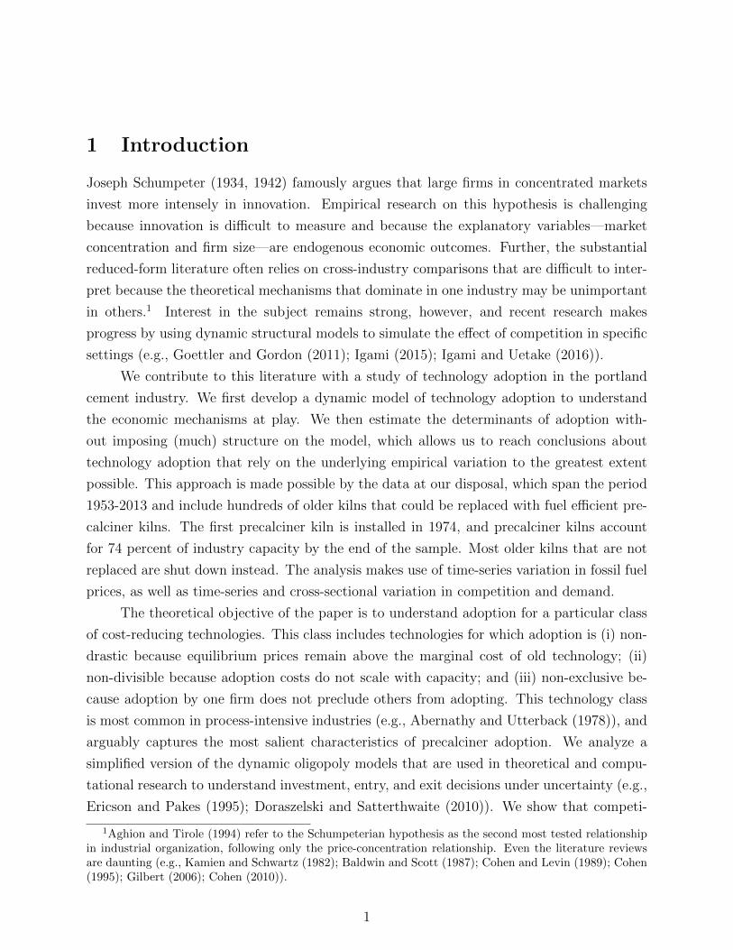
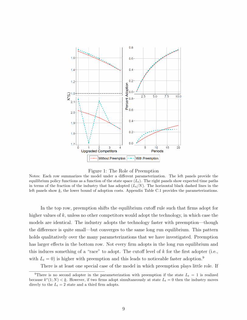
Figure 1 considers two simple numerical examples to illustrate the role of preemption.
The left column shows the optimal policy functions and the right column shows the expected
time path of adoption. The top and bottow rows correspond to the two different param-
eterizations. Each panel features results from the full model (“with preemption”) and an
alternative model that eliminates the preemption incentive (“without preemption”). The
latter model is solved by substituting Π0 for Π1 in the value functions, so that firms do not
consider that adoption changes the subsequent adoption probabilities of competitors.
in the context of entry or exit, because adoption also is a discrete action. Allowing for private shocks meansthat an individual firm essentially treats its rivals as mixing over upgrading and not upgrading.
8
Figure 1: The Role of PreemptionNotes: Each row summarizes the model under a different parameterization. The left panels provide theequilibrium policy functions as a function of the state space (Lt). The right panels show expected time pathsin terms of the fraction of the industry that has adopted (Lt/N). The horizontal black dashed lines in theleft panels show k, the lower bound of adoption costs. Appendix Table C.1 provides the parameterizations.
In the top row, preemption shifts the equilibrium cutoff rule such that firms adopt for
higher values of k, unless no other competitors would adopt the technology, in which case the
models are identical. The industry adopts the technology faster with preemption—though
the difference is quite small—but converges to the same long run equilibrium. This pattern
holds qualitatively over the many parameterizations that we have investigated. Preemption
has larger effects in the bottom row. Not every firm adopts in the long run equilibrium and
this induces something of a “race” to adopt. The cutoff level of k for the first adopter (i.e.,
with Lt = 0) is higher with preemption and this leads to noticeable faster adoption.9
There is at least one special case of the model in which preemption plays little role. If
9There is no second adopter in the parameterization with preemption if the state Lt = 1 is realizedbecause k∗(1;N) < k. However, if two firms adopt simultaneously at state Lt = 0 then the industry movesdirecly to the Lt = 2 state and a third firm adopts.
9
adoption probabilities are small then the benefits of adoption can be approximated as:
b(N) ≈ 1
1− δ(π1 − π0)− k, (6)
Both the preemption and option value terms in equation (5) become small because future
adoption is unlikely, and the equilibrium cutoff rule simplifies to a comparison of stage game
profit with and without adoption. This special case helps motivate the next subsection,
in which we explore the comparative statics of the Nash-Cournot model and develop that
firm scale is a fundamental determinant of technology adoption. It also has bearing on the
empirical exercise because the unconditional probability of precalciner adoption is less than
two percent in a given year.
2.3 Comparative statics and firm size
In this section we focus on the adoption decision of a firm in a situation in which its competi-
tors are unlikely to adopt. We model this decision using a “focal firm” setting, which means
that the focal firm does not integrate out the upgrade probabilities of its rivals. Letting
the inverse demand curve be given by P (Q) = a − Q where Q =∑N
j=1 qj, the equilibrium
markups and quantities of the focal firm facing the adoption decision are given by:
q∗(cx, L;N) = P ∗x (L;N)− cx =a− cx +N(c− cx)
(N + 1)(7)
where again x ∈ 0, 1 denotes the action of the focal firm, and c captures the average
cost of all firms (i.e., c = 1N
[Lc1 + (N − L − 1)c0 + cx]). The profit of the focal firm is
π(cx, L;N) = (q∗(cx, L;N))2 due to the equality of equilibrium markups and quantities.10
Following equation (6), with low adoption probabilities the benefit of adoption can be
approximated as:
b(L;N) ≈ 1
1− δ(π(c1, L;N)− π(c0, L;N)
)− k
=1
1− δ2N
(N + 1)q∗(c, L;N)∆c− k (8)
We refer to the second line as the “static benefit” of adoption because it does not incorporate
10We refer readers to Shapiro (1989) for a more general discussion of the Nash-Cournot model, includingconditions for the existence and uniqueness of equilibrium with nonlinear demand. We employ a unit slopenormalization. This is without loss of generality and all results are robust to demand curve rotations.
10
preemption or the option value. It can be derived in a few lines of algebra starting with
equilibrium markups and quantities, and includes both the magnitude of the cost savings
(∆c = c0 − c1) and the midpoint cost level (c = 12(c0 + c1)). The following comparative
statics are then straight-forward:
Result 1: The static benefit of adoption (i) increases in the cost savings, ∆c; (ii) decreases
in the initial cost level, c0; (iii) increases with industry average costs, c; and (iv) increases
with the inverse demand intercept, a. Further, profit decreases with costs and the number of
firms, but increases with the industry average costs and the inverse demand intercept.
The effect of competitors (i.e., N) on the static benefit is difficult to sign with a
tractable expression because adding a competitor j with costs cj ∈ c0, c1 changes industry
average costs. Consider instead the effect of competitors that have marginal costs cj = c.
(Such competitors do not exist in the full model, but this approach nonetheless conveys
useful intuition.) An additional competitor decreases the benefit that the focal firm receives
from adoption if the following condition holds:(c− cc
)<
(a− cc
)[(N + 1)3 −N(N + 2)2
N2(N + 2)2 − (N + 1)4
](9)
We sketch the derivation in Appendix B. The term in brackets equals 0.29 if N = 2 and
converges to 0.50 as N grows large. The condition holds trivially if L > N/2 because then
the LHS is negative and is exceeded by the RHS (which is positive). In earlier stages of
industry adoption, the condition holds provided that the cost reduction of the technology is
not too great relative to the total surplus created by the industry, which seems plausible in
many settings.11 This leads to a second set of comparative statics:
Result 2: Under condition (9), increasing the number of competitors (i) decreases the static
benefit of adoption; and (ii) decreases the (positive) effect of ∆c on the static benefit.
We pause here to consider that the cost savings of the technology increase the static
benefit of adoption, but that this effect diminishes with the number of firms. This is relevant
for the induced innovation hypothesis because it suggests that competition can mitigate the
11The condition almost surely holds in our empirical application. Because precalciner technology reducesfuel costs by about 30 percent, the maximum value the LHS could take in our application is around (1 −0.85)/0.85 = 0.176. The empirical results of Ganapati, Shapiro and Walker (2016) can be manipulated toobtain (p − c)/c = 1.50 for the cement industry. This provides a lower bound to (a − c)/c. The Ganapati,Shapiro and Walker results use data from the Census of Manufacturers. See Table 2 of the May 2016 draft,which indicates prices of 0.05 and costs of 0.02 (in thousands of 1987 dollars per cubic yard).
11
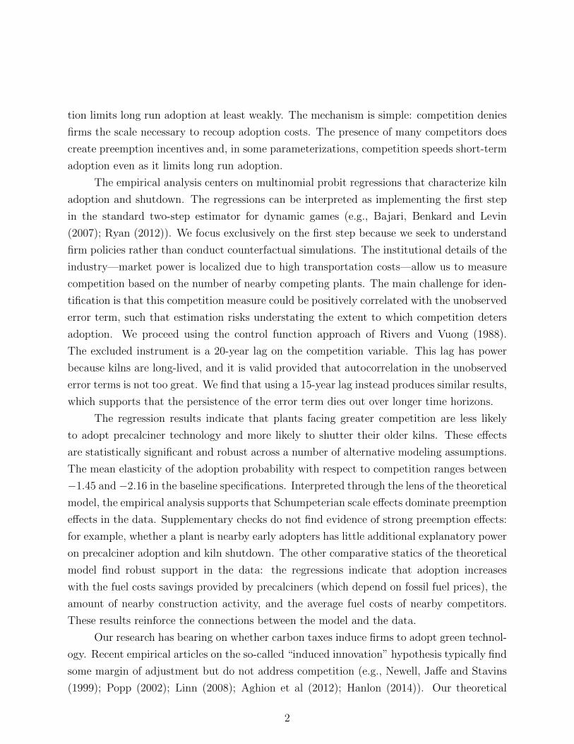
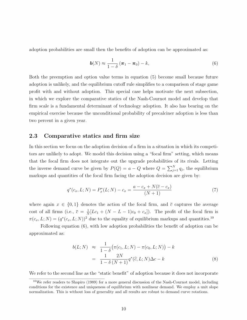
Figure 2: Induced Innovation in the Theoretical ModelNotes: The vertical axis is the adoption probability given Lt = 0 (i.e., F (k∗(0;N))). The horizontal axis is∆c, the magnitude of the cost savings. The different lines show the relationship for N = 1, . . . , 5. AppendixTable C.1 provides the parameterization.
responsiveness of firms to some innovation stimulus. One policy-relevant example is carbon
taxes, which affect adoption incentives by growing the cost difference between “green” and
“dirty” technologies. Figure 2 shows that the comparative static holds in the fully dynamic
version of the model, in which we do not restrict firms to believe its rivals do not upgrade. The
vertical axis is the probability of adoption given Lt = 0. The horizontal axis show different
levels of ∆c. The relationship between adoption and ∆c is provided for N = 1, . . . , 5.
Adoption probabilities increase for larger ∆c, consistent with part (i) of Result 1, but the
increase is less pronounced with large N , consistent with part (ii) of Result 2.
To develop the mechanisms underlying the comparative statics, we reconsider the static
adoption benefits of equation (8) using a first order Taylor Series expansion:
π(c1, L;N)− π(c0, L;N) ≈ − ∂π(c, L;N)
∂c
∣∣∣∣c=c
∆c (10)
where again ∆c = c0 − c1 and c = 12(c0 + c1). This expansion holds with equality if demand
is linear but only differentiability is necessary for a more general analysis. An application of
12
the envelope theorem yields the derivative of the profit function:
−∂π(c, Lt;N)
∂c= q∗i (c, L;N)︸ ︷︷ ︸
Scale Effect
− q∗i (c, L;N)∑k 6=i
∂P ∗
∂qk
∂qk∂qi
∂q∗i∂c︸ ︷︷ ︸
Strategic Effect
(11)
where we use i to index the focal firm. The scale effect captures the standard intuition that
reductions in marginal cost are more profitable if scaled over many units of output (Arrow
(1962)). The magnitude of the scale effect decreases with the number of competitors, and
this creates Schumpeterian dynamics in the full model: competition can deny firms the scale
necessary to recoup adoption costs. By contrast, equilibrium output increases with demand
and industry average costs, and this allows firms to more easily recoup adoption costs. The
strategic effect captures that adoption induces competitors to produce less. Its magnitude
can increase with the number of competitors. With linear demand, the strategic effect
simplifies to(N−1N+1
)q∗(c, L;N), and condition (9) determines the net effect of competition on
the profit derivative.
2.4 Competition and adoption in the dynamic game
Figure 3 provides graphical intuition about the relationship between competition and tech-
nology adoption in the fully dynamic model which allows for preemption. The rows cor-
responds to different parameterizations. The left column provides the equilibrium policy
functions as a function of the state space (Lt). The horizontal black dashed lines show k,
the lower bound of the adoption costs. The right column shows the expected time path of
Lt/N , the fraction of the industry that adopts.
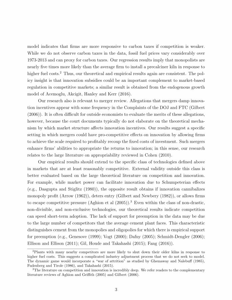
The graph of the policy function in the top row exhibits several notable features. First,
every firm adopts eventually because the equilibrium cutoff levels exceed the lower bound
of the adoption costs (i.e., k∗(Lt) > k for all Lt and N). Second, the policy functions slope
down, for a given N , which indicates that adoption is more likely if fewer competitors have
already adopted. This result happens because with large Lt preemption incentives are weaker
and the stage game benefits are smaller. Third, adding competitors to the model shifts the
policy functions down so that adoption is less likely at any level of Lt. The graph of the time
path shows how these features play out. Adoption happens faster if there are fewer firms,
but regardless an absorbing state is eventually reached in which all firms adopt.
The second row differs because the equilibrium cutoff levels do not always exceed the
lower bound of the adoption cost distribution. Specifically, only three firms adopt if N = 4
13
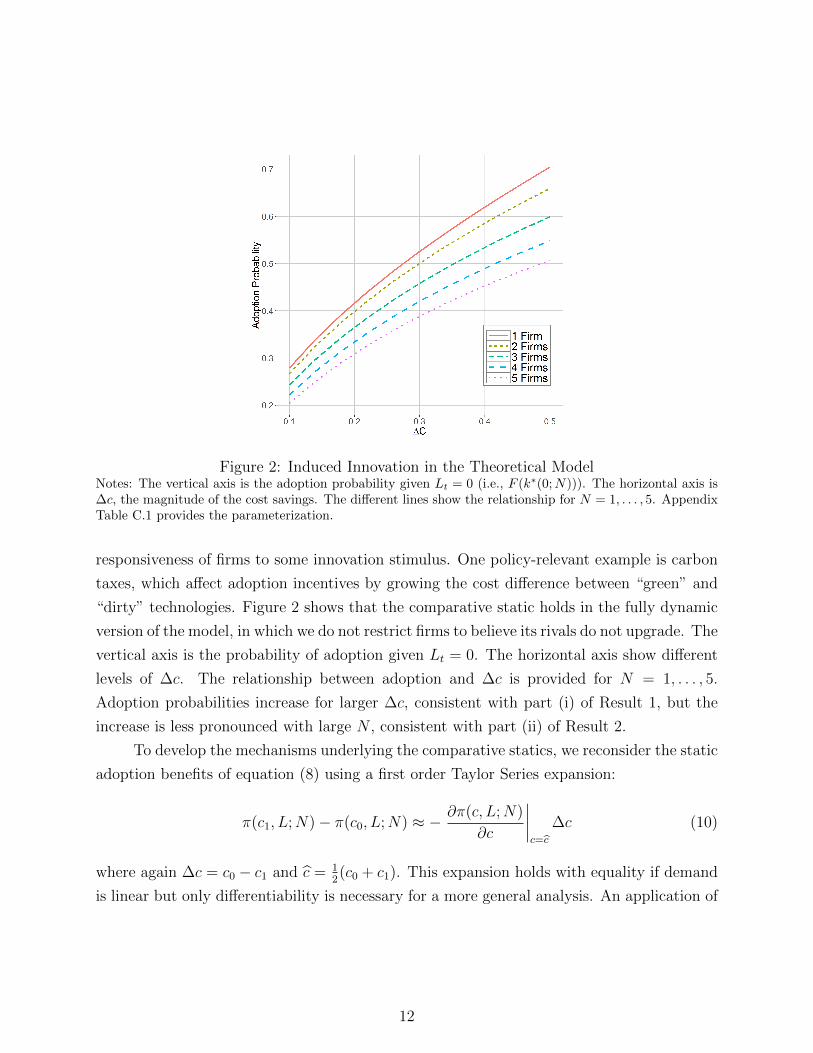
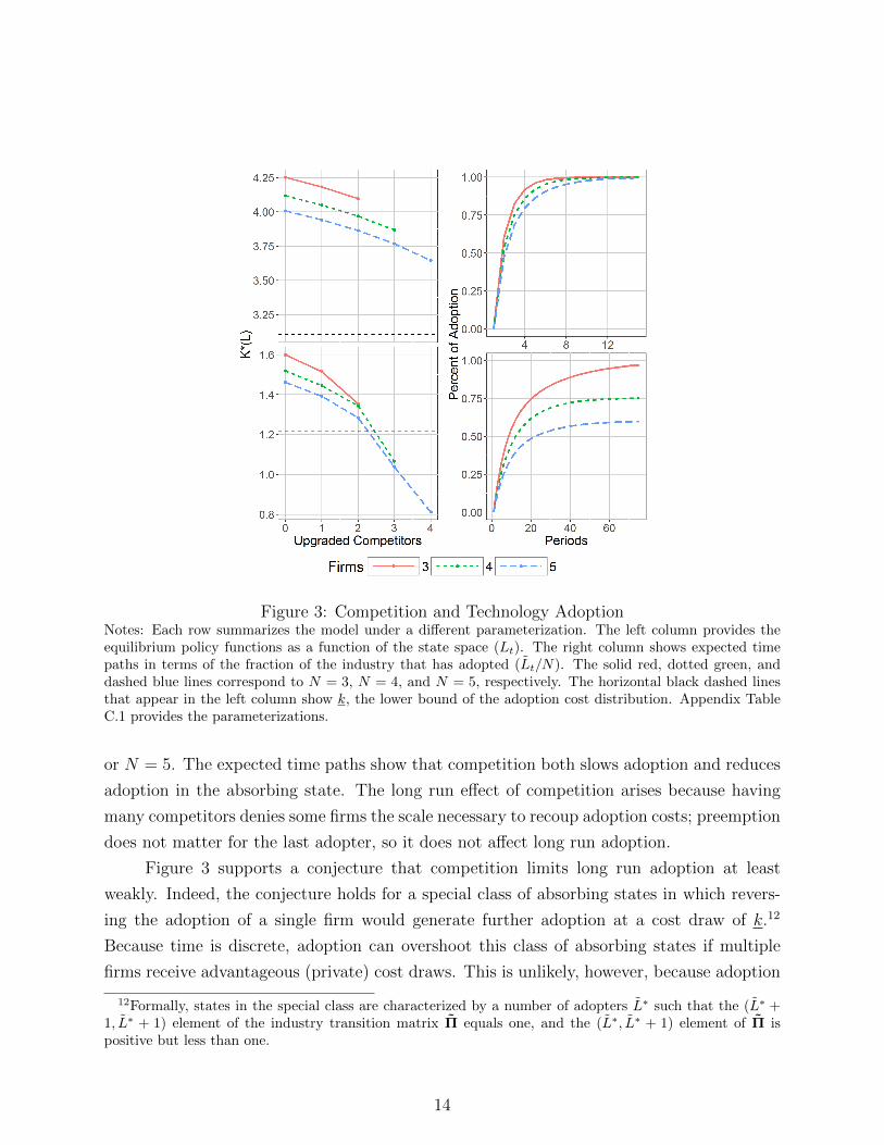
Figure 3: Competition and Technology AdoptionNotes: Each row summarizes the model under a different parameterization. The left column provides theequilibrium policy functions as a function of the state space (Lt). The right column shows expected timepaths in terms of the fraction of the industry that has adopted (Lt/N). The solid red, dotted green, anddashed blue lines correspond to N = 3, N = 4, and N = 5, respectively. The horizontal black dashed linesthat appear in the left column show k, the lower bound of the adoption cost distribution. Appendix TableC.1 provides the parameterizations.
or N = 5. The expected time paths show that competition both slows adoption and reduces
adoption in the absorbing state. The long run effect of competition arises because having
many competitors denies some firms the scale necessary to recoup adoption costs; preemption
does not matter for the last adopter, so it does not affect long run adoption.
Figure 3 supports a conjecture that competition limits long run adoption at least
weakly. Indeed, the conjecture holds for a special class of absorbing states in which revers-
ing the adoption of a single firm would generate further adoption at a cost draw of k.12
Because time is discrete, adoption can overshoot this class of absorbing states if multiple
firms receive advantageous (private) cost draws. This is unlikely, however, because adoption
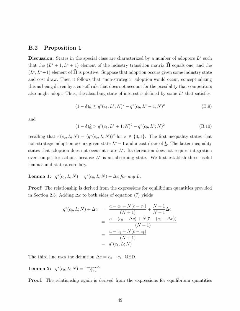
12Formally, states in the special class are characterized by a number of adopters L∗ such that the (L∗ +1, L∗ + 1) element of the industry transition matrix Π equals one, and the (L∗, L∗ + 1) element of Π ispositive but less than one.
14
0
.2
.4
.6
.8
1
Frac
tion
Adop
ting
0
1
2
3
4
5
Num
ber o
f Ado
pter
s
0 3 6 9 12Number of Firms
Number of Adopters Fraction Adopting
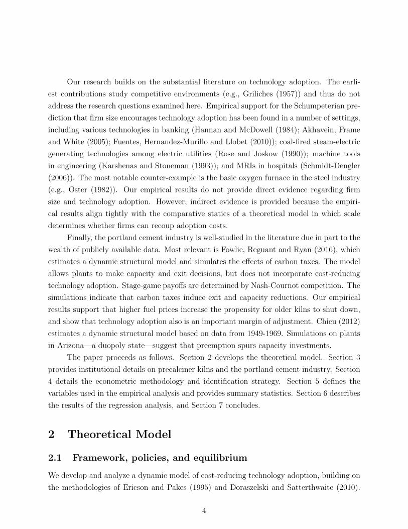
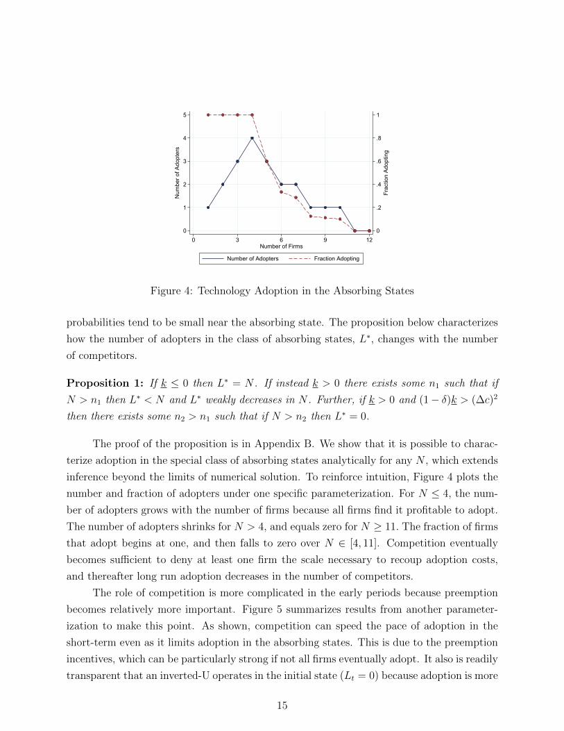
Figure 4: Technology Adoption in the Absorbing States
probabilities tend to be small near the absorbing state. The proposition below characterizes
how the number of adopters in the class of absorbing states, L∗, changes with the number
of competitors.
Proposition 1: If k ≤ 0 then L∗ = N . If instead k > 0 there exists some n1 such that if
N > n1 then L∗ < N and L∗ weakly decreases in N . Further, if k > 0 and (1− δ)k > (∆c)2
then there exists some n2 > n1 such that if N > n2 then L∗ = 0.
The proof of the proposition is in Appendix B. We show that it is possible to charac-
terize adoption in the special class of absorbing states analytically for any N , which extends
inference beyond the limits of numerical solution. To reinforce intuition, Figure 4 plots the
number and fraction of adopters under one specific parameterization. For N ≤ 4, the num-
ber of adopters grows with the number of firms because all firms find it profitable to adopt.
The number of adopters shrinks for N > 4, and equals zero for N ≥ 11. The fraction of firms
that adopt begins at one, and then falls to zero over N ∈ [4, 11]. Competition eventually
becomes sufficient to deny at least one firm the scale necessary to recoup adoption costs,
and thereafter long run adoption decreases in the number of competitors.
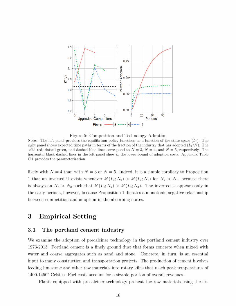
The role of competition is more complicated in the early periods because preemption
becomes relatively more important. Figure 5 summarizes results from another parameter-
ization to make this point. As shown, competition can speed the pace of adoption in the
short-term even as it limits adoption in the absorbing states. This is due to the preemption
incentives, which can be particularly strong if not all firms eventually adopt. It also is readily
transparent that an inverted-U operates in the initial state (Lt = 0) because adoption is more
15
Figure 5: Competition and Technology AdoptionNotes: The left panel provides the equilibrium policy functions as a function of the state space (Lt). Theright panel shows expected time paths in terms of the fraction of the industry that has adopted (Lt/N). Thesolid red, dotted green, and dashed blue lines correspond to N = 3, N = 4, and N = 5, respectively. Thehorizontal black dashed lines in the left panel show k, the lower bound of adoption costs. Appendix TableC.1 provides the parameterization.
likely with N = 4 than with N = 3 or N = 5. Indeed, it is a simple corollary to Proposition
1 that an inverted-U exists whenever k∗(Lt;N2) > k∗(Lt;N1) for N2 > N1, because there
is always an N3 > N2 such that k∗(Lt;N2) > k∗(Lt;N3). The inverted-U appears only in
the early periods, however, because Proposition 1 dictates a monotonic negative relationship
between competition and adoption in the absorbing states.
3 Empirical Setting
3.1 The portland cement industry
We examine the adoption of precalciner technology in the portland cement industry over
1973-2013. Portland cement is a finely ground dust that forms concrete when mixed with
water and coarse aggregates such as sand and stone. Concrete, in turn, is an essential
input to many construction and transportation projects. The production of cement involves
feeding limestone and other raw materials into rotary kilns that reach peak temperatures of
1400-1450 Celsius. Fuel costs account for a sizable portion of overall revenues.
Plants equipped with precalciner technology preheat the raw materials using the ex-
16
haust gases of the kiln combined with heat from a supplementary combustion chamber,
which reduces production energy requirements by 25-35 percent by allowing an important
chemical reaction (calcination) to begin before raw materials enter the kiln. This reduces the
requisite kiln length and requires a complete plant retrofit. Cement producers outsource kiln
design to one of several industrial architecture firms with expertise in cement. The physical
component is not especially demanding—many industrial construction firms can manage the
steel plates, refractory linings, and duct work—but total design and installation costs are
large. To provide an order of magnitude, publicly-available estimates place the total cost of
building a modern cement plant around $800 million.13
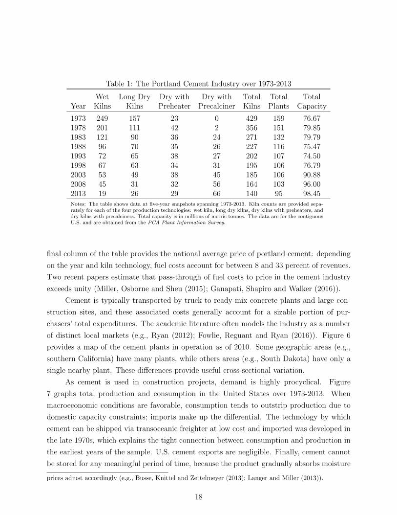
Table 1 tracks precalciner kiln adoption over time. In 1973, nearly all plants used inef-
ficient wet and long dry kilns. A small number of plants utilized preheater technology, which
recycles exhaust gases without a supplementary combustion chamber, but no plant used
precalciner technology. Over the ensuing four decades, the number of wet kilns decreased
from 249 to 19 and the number of long dry kilns decreased from 157 to 26. Shuttered kilns
typically remain on site because they are costly to relocate, but most of the supporting equip-
ment can be repurposed profitably. By the final year of data 2013, there are 66 precalciner
kilns in operation and these account for 74 percent of industry capacity.
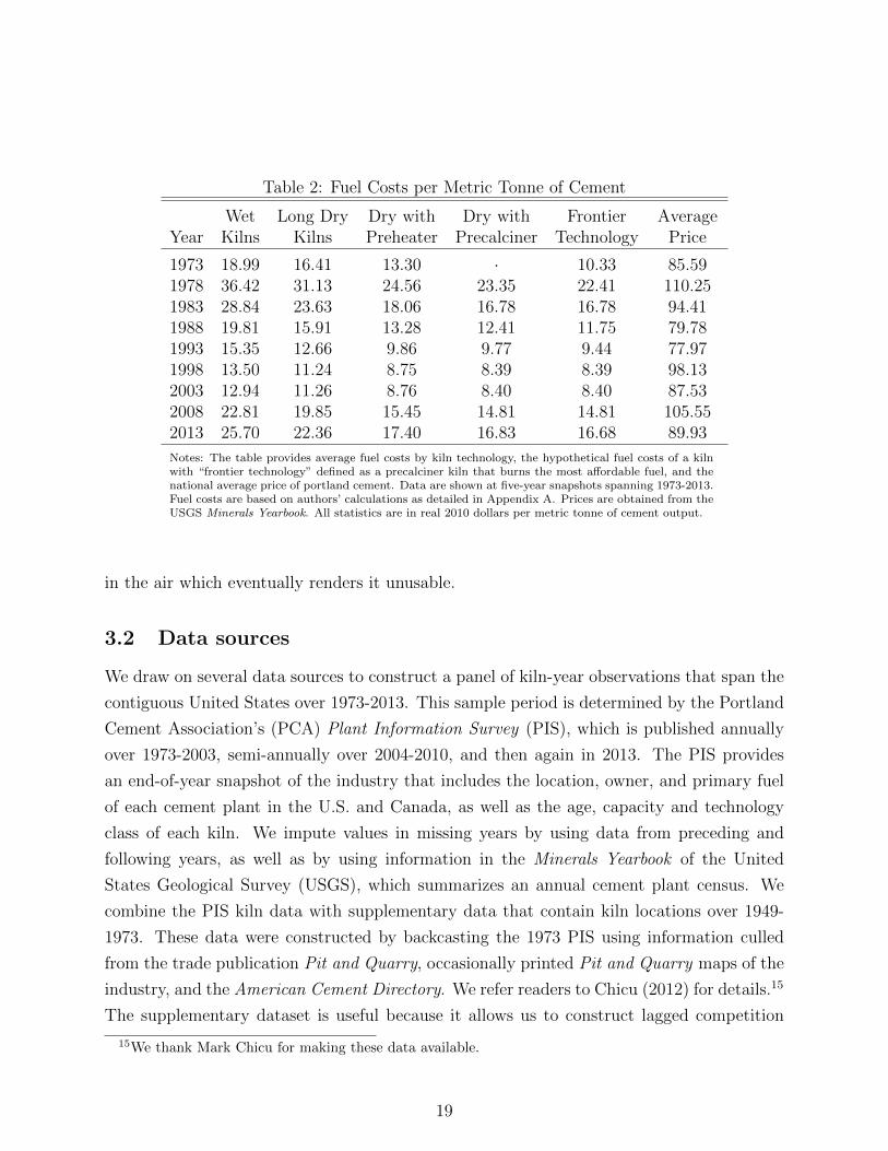
Table 2 provides the average fuel costs among kilns in each technology class, again at
five-year intervals over the sample period. These costs are obtained based on kiln efficiency
and the price/mBtu of the primary fossil fuel used. The changes within kiln technology
classes over time are driven primarily by exogenous fluctuations in natural gas and coal
prices, which provides a key source of variation that we exploit in the estimation. This
feature of the data can be interpreted further as providing a natural experiment as to how
firms would respond to carbon taxes, which change the price of fossil fuels.
Table 2 also provides the fuel costs of the “frontier technology,” which we define as
a precalciner kiln that burns the most affordable fuel. The difference between a kiln’s fuel
cost and that of the frontier technology – a measure of the fuel cost savings available from
precalciner adoption – is an empirical analog to the ∆c term in the motivating theory. Fuel
cost savings tend to be large when fossil fuel prices (and thus fuel costs) are high.14 The
13CEMBUREAU, the European cement association, places construction costs for a one million metrictonne plant at around three years of revenue, and estimates annual total costs of around $200 million.A study by The Carbon War Room (2011), an environmental action group, places profit margins at 33percent given a per-tonne price of $100. Putting these facts together, our $800 million number is calculatedas $200 × 1.33 × 3 = $798 ≈ $800. For the CEMBUREAU estimate, see http://www.cembureau.be/
about-cement/cement-industry-main-characteristics14There is a well known analogy in the automobile industry: the driving cost of vehicles with low miles-
per-gallon (MPG) is more sensitive to the gasoline price than that of high MPG vehicles, and automobile
17
Table 1: The Portland Cement Industry over 1973-2013
Wet Long Dry Dry with Dry with Total Total TotalYear Kilns Kilns Preheater Precalciner Kilns Plants Capacity
1973 249 157 23 0 429 159 76.671978 201 111 42 2 356 151 79.851983 121 90 36 24 271 132 79.791988 96 70 35 26 227 116 75.471993 72 65 38 27 202 107 74.501998 67 63 34 31 195 106 76.792003 53 49 38 45 185 106 90.882008 45 31 32 56 164 103 96.002013 19 26 29 66 140 95 98.45Notes: The table shows data at five-year snapshots spanning 1973-2013. Kiln counts are provided sepa-rately for each of the four production technologies: wet kiln, long dry kilns, dry kilns with preheaters, anddry kilns with precalciners. Total capacity is in millions of metric tonnes. The data are for the contiguousU.S. and are obtained from the PCA Plant Information Survey.
final column of the table provides the national average price of portland cement: depending
on the year and kiln technology, fuel costs account for between 8 and 33 percent of revenues.
Two recent papers estimate that pass-through of fuel costs to price in the cement industry
exceeds unity (Miller, Osborne and Sheu (2015); Ganapati, Shapiro and Walker (2016)).
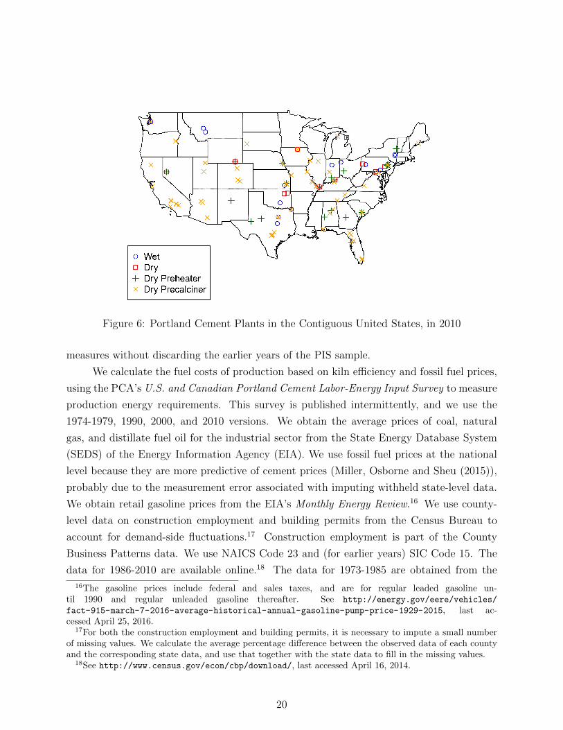
Cement is typically transported by truck to ready-mix concrete plants and large con-
struction sites, and these associated costs generally account for a sizable portion of pur-
chasers’ total expenditures. The academic literature often models the industry as a number
of distinct local markets (e.g., Ryan (2012); Fowlie, Reguant and Ryan (2016)). Figure 6
provides a map of the cement plants in operation as of 2010. Some geographic areas (e.g.,
southern California) have many plants, while others areas (e.g., South Dakota) have only a
single nearby plant. These differences provide useful cross-sectional variation.
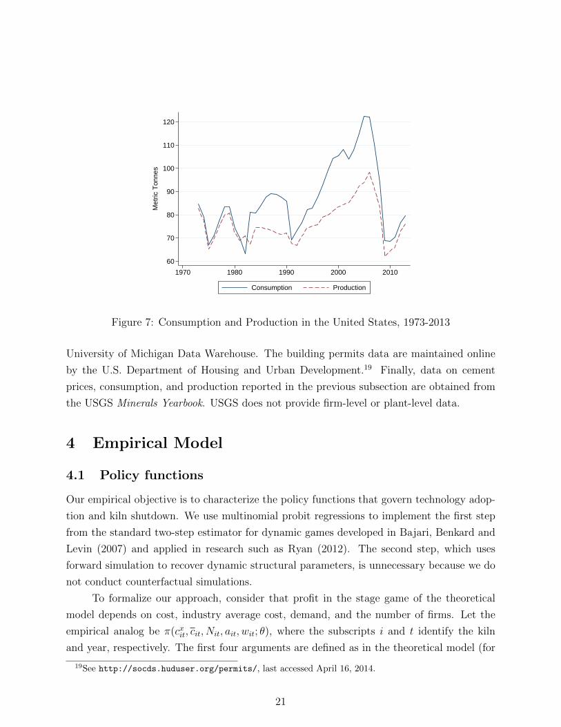
As cement is used in construction projects, demand is highly procyclical. Figure
7 graphs total production and consumption in the United States over 1973-2013. When
macroeconomic conditions are favorable, consumption tends to outstrip production due to
domestic capacity constraints; imports make up the differential. The technology by which
cement can be shipped via transoceanic freighter at low cost and imported was developed in
the late 1970s, which explains the tight connection between consumption and production in
the earliest years of the sample. U.S. cement exports are negligible. Finally, cement cannot
be stored for any meaningful period of time, because the product gradually absorbs moisture
prices adjust accordingly (e.g., Busse, Knittel and Zettelmeyer (2013); Langer and Miller (2013)).
18
Table 2: Fuel Costs per Metric Tonne of Cement
Wet Long Dry Dry with Dry with Frontier AverageYear Kilns Kilns Preheater Precalciner Technology Price
Notes: The table provides average fuel costs by kiln technology, the hypothetical fuel costs of a kilnwith “frontier technology” defined as a precalciner kiln that burns the most affordable fuel, and thenational average price of portland cement. Data are shown at five-year snapshots spanning 1973-2013.Fuel costs are based on authors’ calculations as detailed in Appendix A. Prices are obtained from theUSGS Minerals Yearbook. All statistics are in real 2010 dollars per metric tonne of cement output.
in the air which eventually renders it unusable.
3.2 Data sources
We draw on several data sources to construct a panel of kiln-year observations that span the
contiguous United States over 1973-2013. This sample period is determined by the Portland
Cement Association’s (PCA) Plant Information Survey (PIS), which is published annually
over 1973-2003, semi-annually over 2004-2010, and then again in 2013. The PIS provides
an end-of-year snapshot of the industry that includes the location, owner, and primary fuel
of each cement plant in the U.S. and Canada, as well as the age, capacity and technology
class of each kiln. We impute values in missing years by using data from preceding and
following years, as well as by using information in the Minerals Yearbook of the United
States Geological Survey (USGS), which summarizes an annual cement plant census. We
combine the PIS kiln data with supplementary data that contain kiln locations over 1949-
1973. These data were constructed by backcasting the 1973 PIS using information culled
from the trade publication Pit and Quarry, occasionally printed Pit and Quarry maps of the
industry, and the American Cement Directory. We refer readers to Chicu (2012) for details.15
The supplementary dataset is useful because it allows us to construct lagged competition
15We thank Mark Chicu for making these data available.
19
Figure 6: Portland Cement Plants in the Contiguous United States, in 2010
measures without discarding the earlier years of the PIS sample.
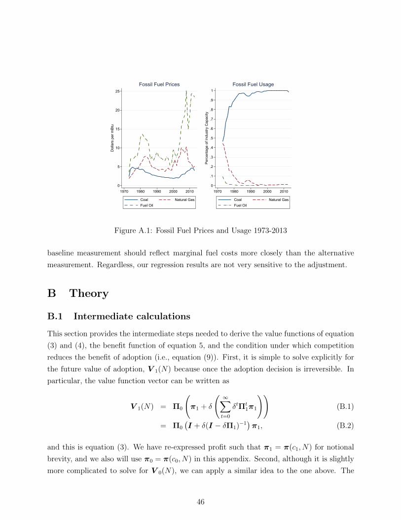
We calculate the fuel costs of production based on kiln efficiency and fossil fuel prices,
using the PCA’s U.S. and Canadian Portland Cement Labor-Energy Input Survey to measure
production energy requirements. This survey is published intermittently, and we use the
1974-1979, 1990, 2000, and 2010 versions. We obtain the average prices of coal, natural
gas, and distillate fuel oil for the industrial sector from the State Energy Database System
(SEDS) of the Energy Information Agency (EIA). We use fossil fuel prices at the national
level because they are more predictive of cement prices (Miller, Osborne and Sheu (2015)),
probably due to the measurement error associated with imputing withheld state-level data.
We obtain retail gasoline prices from the EIA’s Monthly Energy Review.16 We use county-
level data on construction employment and building permits from the Census Bureau to
account for demand-side fluctuations.17 Construction employment is part of the County
Business Patterns data. We use NAICS Code 23 and (for earlier years) SIC Code 15. The
data for 1986-2010 are available online.18 The data for 1973-1985 are obtained from the
16The gasoline prices include federal and sales taxes, and are for regular leaded gasoline un-til 1990 and regular unleaded gasoline thereafter. See http://energy.gov/eere/vehicles/
fact-915-march-7-2016-average-historical-annual-gasoline-pump-price-1929-2015, last ac-cessed April 25, 2016.
17For both the construction employment and building permits, it is necessary to impute a small numberof missing values. We calculate the average percentage difference between the observed data of each countyand the corresponding state data, and use that together with the state data to fill in the missing values.
18See http://www.census.gov/econ/cbp/download/, last accessed April 16, 2014.
20
60
70
80
90
100
110
120
Met
ric T
onne
s
1970 1980 1990 2000 2010
Consumption Production
Figure 7: Consumption and Production in the United States, 1973-2013
University of Michigan Data Warehouse. The building permits data are maintained online
by the U.S. Department of Housing and Urban Development.19 Finally, data on cement
prices, consumption, and production reported in the previous subsection are obtained from
the USGS Minerals Yearbook. USGS does not provide firm-level or plant-level data.
4 Empirical Model
4.1 Policy functions
Our empirical objective is to characterize the policy functions that govern technology adop-
tion and kiln shutdown. We use multinomial probit regressions to implement the first step
from the standard two-step estimator for dynamic games developed in Bajari, Benkard and
Levin (2007) and applied in research such as Ryan (2012). The second step, which uses
forward simulation to recover dynamic structural parameters, is unnecessary because we do
not conduct counterfactual simulations.
To formalize our approach, consider that profit in the stage game of the theoretical
model depends on cost, industry average cost, demand, and the number of firms. Let the
empirical analog be π(cxit, cit, Nit, ait, wit; θ), where the subscripts i and t identify the kiln
and year, respectively. The first four arguments are defined as in the theoretical model (for
19See http://socds.huduser.org/permits/, last accessed April 16, 2014.
21
x = 0, 1), wit is a vector of controls, and θ is a vector of parameters. Define the empirical
“benefit of adoption” for a producer with an old kiln as:
where zit is an instrument that is excluded from the producers’ maximization problem,
φNt is specified the same way as φA
t and φSt , and vit is a reduced-form error term. For
notational convenience, we collect the exogenous variables in the vector Xit. We assume that
(Xit, uAit, u
Sit, vit) is i.i.d. Further, let (uAit, u
Sit, vit) have a mean-zero joint normal distribution,
conditional on Xit, with the finite positive definite covariance matrix:
Ω ≡
σAuu σAS
uu σAvu
σASuu σS
uu σSvu
σAvu σS
vu σvv
(16)
Endogeneity is present if the reduced-form error term is correlated with the stochastic
shocks (specifically, if σAvu 6= 0 or σS
vu 6= 0). Using the joint normality assumption, the
stochastic shocks can be rewritten as ukit = vitλk + ηkit for k ∈ A, S, where λk = σk
vu/σvv
and ηkit = ukit − vitλk. If a suitable control function is used as a proxy for the reduced-form
error, vit, then the measure of competition is orthogonal to the remaining error terms (Rivers
and Vuong (1988)). Estimation proceeds in two stages:
1. OLS estimation of Nit on the exogenous regressors. This obtains an estimate of the
reduced-form error term that we denote vit.
2. Maximum likelihood estimation of the multinomial probit equations using vit as a
control function. Differences between vit and vit are normally distributed and thus
compatible with the distributional assumptions of the multinomial probit model.
The second-stage standard errors can be adjusted to account for the presence of the esti-
mation of the control function using a multi-step procedure based on the minimum distance
estimator of Amemiya (1978) and Newey (1987). This adjustment has virtually no effect in
our application, however, so we report simpler standard errors that are clustered at the kiln
level to correct for autocorrelation.
4.3 Identification and instrument
The theoretical model indicates that technology adoption is more likely under favorable
profit conditions, and greater profit generally supports more competitors. It follows that any
correlation between uAit and vit is likely positive, and this allows the bias to be signed: the
basic probit estimator is likely to understate the extent that competition deters technology
23
adoption. Similar logic applies to kiln shutdown, although our regression results indicate
that bias in that equation is empirically less important.
Finding an instrument to correct endogeneity bias is not straightforward. Our set-
ting differs from more standard industrial organization applications that involve demand or
supply estimation, and for which cost or demand shocks respectively are valid instruments.
Because both demand and cost enter the profit function, neither provides the requisite ex-
ogenous variation. We proceed instead under an identifying assumption that competitive
conditions exhibit greater autocorrelation than the unobserved profit shocks:
limT→∞
Cov(uAit, uAi,t−T )
Cov(Nit, Ni,t−T )= 0 (17)
That Nit exhibits a high degree of persistence is clear from the data: a regression of Nit on
Ni,t−1 and all of the exogenous variables of equation (13) yields a coefficient on the lag of
0.70 (p-value of 0.000). This persistence is due to the longevity of kilns, which are on average
40 years old upon retirement. The degree of persistence in the unobserved profit shock is
impossible to evaluate independently, but the frequent changes in observed cost and demand
conditions (e.g., see Table 2 and Figure 7) provide some support for this assumption.
Under equation (17), if a lagged version of the competition measure is used as an
instrument then bias converges to zero with the length of the lag. We use a lag of 20 years,
which exploits the decades of pre-adoption data collected in Chicu (2012). The instrument
has power and generates F -statistics between 2,700 and 3,800 in our baseline regressions.
Some bias remains if Cov(uAit, uAi,t−20) 6= 0. This possibility motivates robustness checks in
which we use alternative instruments based on respective lags of 15, 10, and 5 years. The
results support that the persistence of the error term dies out over longer time horizons.
Other sources of endogeneity seem unlikely. Exogeneity of the demand controls is likely
to be reasonable. Technology decisions within a market are not likely to drive demand,
because cement represents a small fraction of total construction costs. Endogeneity in fossil
fuel prices could arise if increases in fuel demand from cement plants led to price increases
in the fuel market. However, any such feedback should be small because cement accounts
for a fraction of the fossil fuels used in the United States. Consistent with this argument,
bituminous coal prices do not exhibit the same pro-cyclical variation as cement demand.
Industry costs (i.e., cit) incorporate previous technology decisions and thus could be related
to the unobserved profit shocks. However, we obtain similar results if we instrument for
industry costs using a 20-year lag on the count of nearby precalciners, and the main results
also are robust to the exclusion of industry costs as an independent variable.
24
5 Variables and summary statistics
5.1 Variables
We calculate the fuel costs of each kiln based on its energy requirements and the price of
the primary fuel:
Fuel Costjt = Primary Fuel Pricejt × Energy Requirementsjt
where the fuel price is in dollars per mBtu and the energy requirements are in mBtu per
metric tonne of clinker. We obtain the energy requirements from the PCA labor-energy
input surveys. Details on this calculation are provided in Appendix A. The cost savings
that would be realized by adopting precalciner technology are the difference between the fuel
costs of the kiln and those of the technology frontier, which we define based on the energy
requirements of a precalciner kiln using the most affordable fuel. This difference provides
the empirical proxy for the ∆c term that appears in the theoretical model.
We measure competition based on plant locations and gasoline prices. We first define a
distance metric as the multiplicative product of miles and a gasoline price index that equals
one in the year 2000. We then calculate the number of competing plants within a distance
radius of 400 to obtain an empirical proxy for Nit. This radius is motivated by prior findings
that 80-90 percent of portland cement is trucked less than 200 miles (Census Bureau (1977);
Miller and Osborne (2014)), so that plants separated by a distance of more than 400 are
unlikely to compete for customers.20 We exclude plants owned by the same firm from the
competition measure, though few such plants exist within the specified radius. We also use
the distance radius to calculate the industry costs for each plant (i.e., cit), defined as the
average costs of all other plants with the radius. The competition and industry cost variables
use the location of plants as of the prior year.
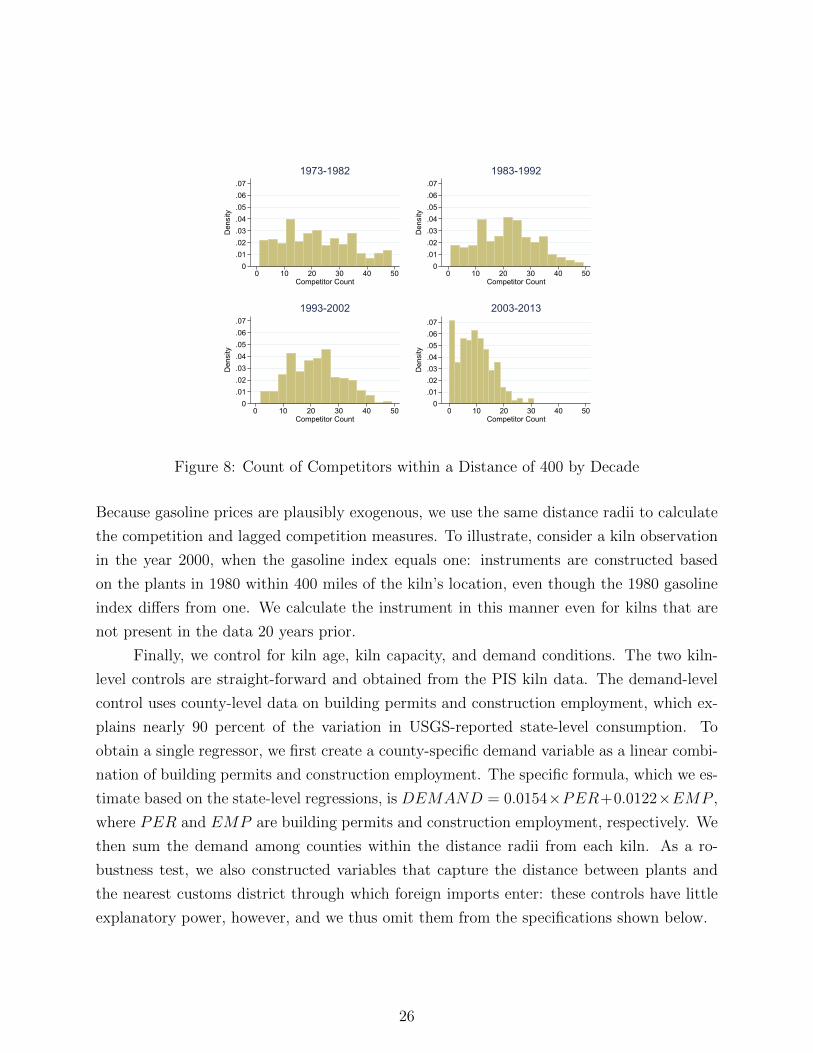
Figure 8 provides separate decadal histograms for the count of nearby competitors.
Cross-sectional variation is due to plant location dispersion, while inter-temporal variation
arises due to gasoline price fluctuations, plant closures, and (infrequent) plant entry. We use
instruments based on the locations of plants 20 years prior to the observation in question.
20Our treatment of distance reflects the predominant role of trucking in cement distribution. A fractionof cement is shipped to terminals by train (6 percent in 2010) or barge (11 percent in 2010), and only thenis trucked to customers. Some plants may therefore be closer than our metric indicates if, for example,both are located on the same river system. Straight-line miles are highly correlated with both driving milesand driving time and, consistent with this, previously published empirical results on the industry are notsensitive to which of these measures is employed (e.g., Miller and Osborne (2014)).
25
0.01.02.03.04.05.06.07
Den
sity
0 10 20 30 40 50Competitor Count
1973-1982
0.01.02.03.04.05.06.07
Den
sity
0 10 20 30 40 50Competitor Count
1983-1992
0.01.02.03.04.05.06.07
Den
sity
0 10 20 30 40 50Competitor Count
1993-2002
0.01.02.03.04.05.06.07
Den
sity
0 10 20 30 40 50Competitor Count
2003-2013
Figure 8: Count of Competitors within a Distance of 400 by Decade
Because gasoline prices are plausibly exogenous, we use the same distance radii to calculate
the competition and lagged competition measures. To illustrate, consider a kiln observation
in the year 2000, when the gasoline index equals one: instruments are constructed based
on the plants in 1980 within 400 miles of the kiln’s location, even though the 1980 gasoline
index differs from one. We calculate the instrument in this manner even for kilns that are
not present in the data 20 years prior.
Finally, we control for kiln age, kiln capacity, and demand conditions. The two kiln-
level controls are straight-forward and obtained from the PIS kiln data. The demand-level
control uses county-level data on building permits and construction employment, which ex-
plains nearly 90 percent of the variation in USGS-reported state-level consumption. To
obtain a single regressor, we first create a county-specific demand variable as a linear combi-
nation of building permits and construction employment. The specific formula, which we es-
timate based on the state-level regressions, is DEMAND = 0.0154×PER+0.0122×EMP ,
where PER and EMP are building permits and construction employment, respectively. We
then sum the demand among counties within the distance radii from each kiln. As a ro-
bustness test, we also constructed variables that capture the distance between plants and
the nearest customs district through which foreign imports enter: these controls have little
explanatory power, however, and we thus omit them from the specifications shown below.
26
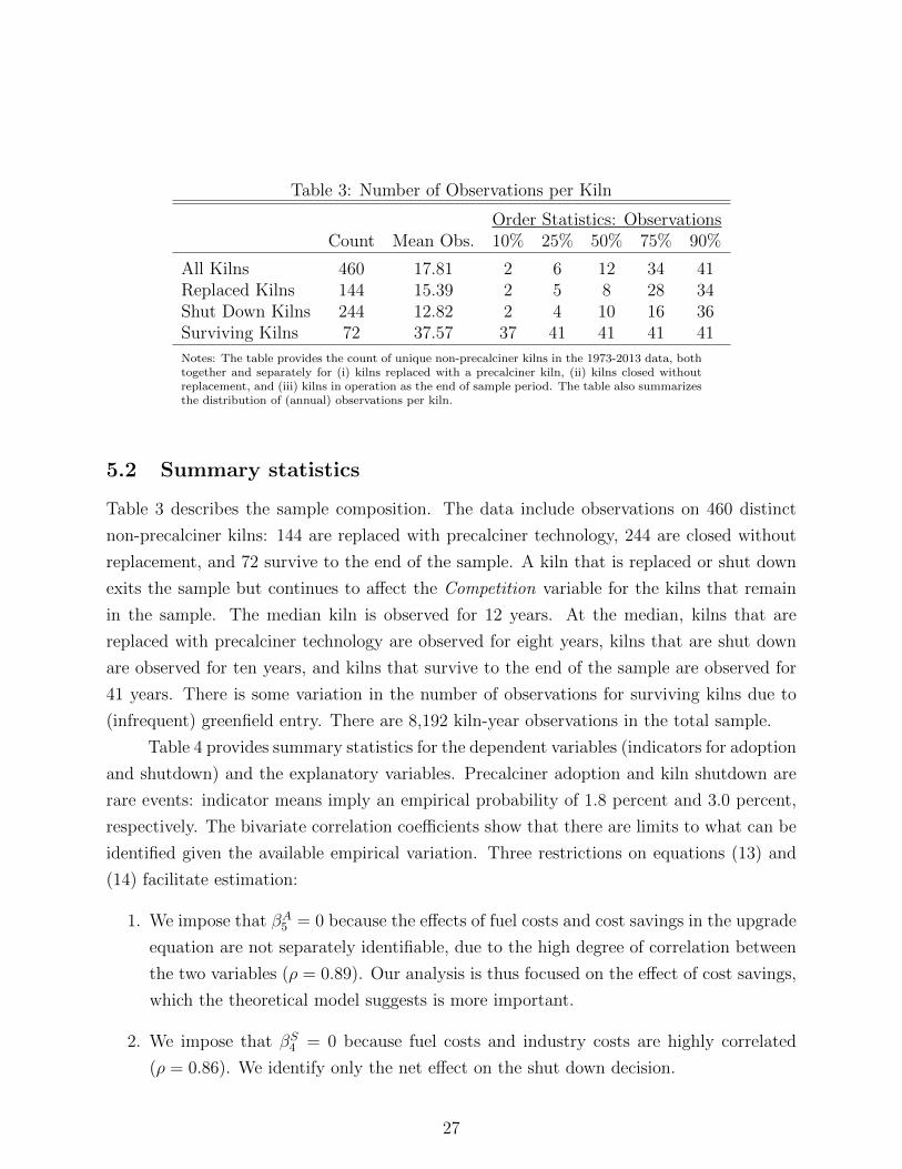
Table 3: Number of Observations per Kiln
Order Statistics: ObservationsCount Mean Obs. 10% 25% 50% 75% 90%
Notes: The table provides the count of unique non-precalciner kilns in the 1973-2013 data, bothtogether and separately for (i) kilns replaced with a precalciner kiln, (ii) kilns closed withoutreplacement, and (iii) kilns in operation as the end of sample period. The table also summarizesthe distribution of (annual) observations per kiln.
5.2 Summary statistics
Table 3 describes the sample composition. The data include observations on 460 distinct
non-precalciner kilns: 144 are replaced with precalciner technology, 244 are closed without
replacement, and 72 survive to the end of the sample. A kiln that is replaced or shut down
exits the sample but continues to affect the Competition variable for the kilns that remain
in the sample. The median kiln is observed for 12 years. At the median, kilns that are
replaced with precalciner technology are observed for eight years, kilns that are shut down
are observed for ten years, and kilns that survive to the end of the sample are observed for
41 years. There is some variation in the number of observations for surviving kilns due to
(infrequent) greenfield entry. There are 8,192 kiln-year observations in the total sample.
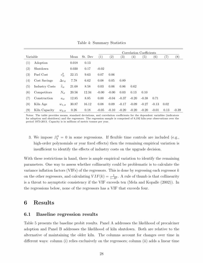
Table 4 provides summary statistics for the dependent variables (indicators for adoption
and shutdown) and the explanatory variables. Precalciner adoption and kiln shutdown are
rare events: indicator means imply an empirical probability of 1.8 percent and 3.0 percent,
respectively. The bivariate correlation coefficients show that there are limits to what can be
identified given the available empirical variation. Three restrictions on equations (13) and
(14) facilitate estimation:
1. We impose that βA5 = 0 because the effects of fuel costs and cost savings in the upgrade
equation are not separately identifiable, due to the high degree of correlation between
the two variables (ρ = 0.89). Our analysis is thus focused on the effect of cost savings,
which the theoretical model suggests is more important.
2. We impose that βS4 = 0 because fuel costs and industry costs are highly correlated
(ρ = 0.86). We identify only the net effect on the shut down decision.
27
Table 4: Summary Statistics
Correlation CoefficientsVariable Mean St. Dev (1) (2) (3) (4) (5) (6) (7) (8)
(1) Adoption 0.018 0.13
(2) Shutdown 0.030 0.17 -0.02
(3) Fuel Cost c0it 22.15 9.63 0.07 0.06
(4) Cost Savings ∆cit 7.78 6.62 0.08 0.05 0.89
(5) Industry Costs cit 21.68 8.58 0.03 0.06 0.86 0.62
Notes: The table provides means, standard deviations, and correlation coefficients for the dependent variables (indicatorsfor adoption and shutdown) and the regressors. The regression sample is comprised of 8,192 kiln-year observations over theperiod 1973-2013. Capacity is in millions of metric tonnes per year.
3. We impose βA4 = 0 in some regressions. If flexible time controls are included (e.g.,
high-order polynomials or year fixed effects) then the remaining empirical variation is
insufficient to identify the effects of industry costs on the upgrade decision.
With these restrictions in hand, there is ample empirical variation to identify the remaining
parameters. One way to assess whether collinearity could be problematic is to calculate the
variance inflation factors (VIFs) of the regressors. This is done by regressing each regressor k
on the other regressors, and calculating V IF (k) = 11−R2 . A rule of thumb is that collinearity
is a threat to asymptotic consistency if the VIF exceeds ten (Mela and Kopalle (2002)). In
the regressions below, none of the regressors has a VIF that exceeds four.
6 Results
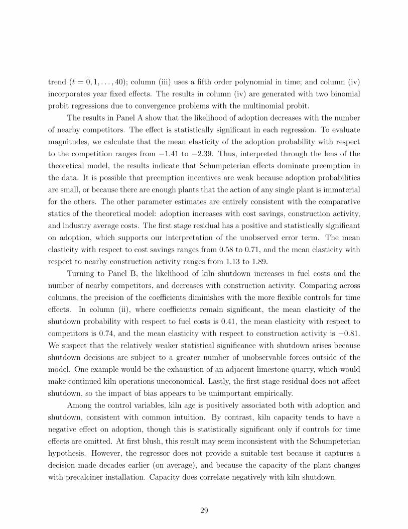
6.1 Baseline regression results
Table 5 presents the baseline probit results. Panel A addresses the likelihood of precalciner
adoption and Panel B addresses the likelihood of kiln shutdown. Both are relative to the
alternative of maintaining the older kiln. The columns account for changes over time in
different ways: column (i) relies exclusively on the regressors; column (ii) adds a linear time
28
trend (t = 0, 1, . . . , 40); column (iii) uses a fifth order polynomial in time; and column (iv)
incorporates year fixed effects. The results in column (iv) are generated with two binomial
probit regressions due to convergence problems with the multinomial probit.
The results in Panel A show that the likelihood of adoption decreases with the number
of nearby competitors. The effect is statistically significant in each regression. To evaluate
magnitudes, we calculate that the mean elasticity of the adoption probability with respect
to the competition ranges from −1.41 to −2.39. Thus, interpreted through the lens of the
theoretical model, the results indicate that Schumpeterian effects dominate preemption in
the data. It is possible that preemption incentives are weak because adoption probabilities
are small, or because there are enough plants that the action of any single plant is immaterial
for the others. The other parameter estimates are entirely consistent with the comparative
statics of the theoretical model: adoption increases with cost savings, construction activity,
and industry average costs. The first stage residual has a positive and statistically significant
on adoption, which supports our interpretation of the unobserved error term. The mean
elasticity with respect to cost savings ranges from 0.58 to 0.71, and the mean elasticity with
respect to nearby construction activity ranges from 1.13 to 1.89.
Turning to Panel B, the likelihood of kiln shutdown increases in fuel costs and the
number of nearby competitors, and decreases with construction activity. Comparing across
columns, the precision of the coefficients diminishes with the more flexible controls for time
effects. In column (ii), where coefficients remain significant, the mean elasticity of the
shutdown probability with respect to fuel costs is 0.41, the mean elasticity with respect to
competitors is 0.74, and the mean elasticity with respect to construction activity is −0.81.
We suspect that the relatively weaker statistical significance with shutdown arises because
shutdown decisions are subject to a greater number of unobservable forces outside of the
model. One example would be the exhaustion of an adjacent limestone quarry, which would
make continued kiln operations uneconomical. Lastly, the first stage residual does not affect
shutdown, so the impact of bias appears to be unimportant empirically.
Among the control variables, kiln age is positively associated both with adoption and
shutdown, consistent with common intuition. By contrast, kiln capacity tends to have a
negative effect on adoption, though this is statistically significant only if controls for time
effects are omitted. At first blush, this result may seem inconsistent with the Schumpeterian
hypothesis. However, the regressor does not provide a suitable test because it captures a
decision made decades earlier (on average), and because the capacity of the plant changes
with precalciner installation. Capacity does correlate negatively with kiln shutdown.
29
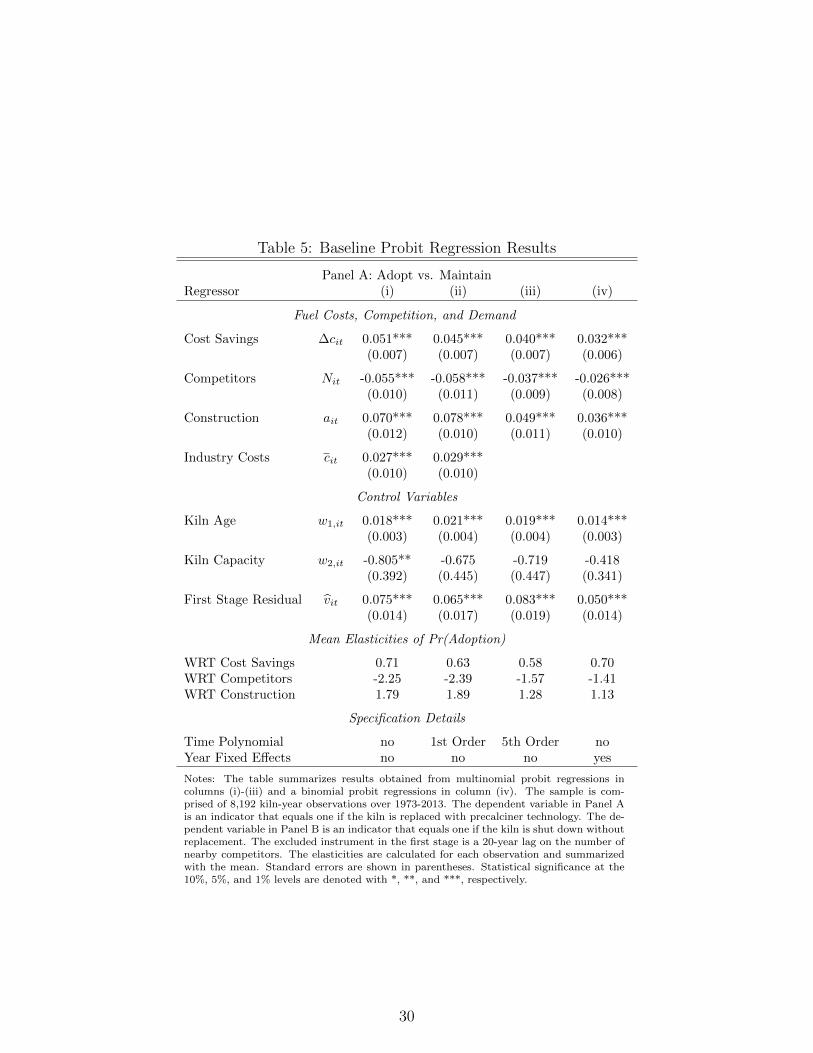
Table 5: Baseline Probit Regression Results
Panel A: Adopt vs. MaintainRegressor (i) (ii) (iii) (iv)
Time Polynomial no 1st Order 5th Order noYear Fixed Effects no no no yes
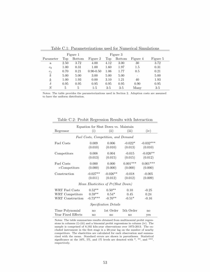
Notes: The table summarizes results obtained from multinomial probit regressions incolumns (i)-(iii) and a binomial probit regressions in column (iv). The sample is com-prised of 8,192 kiln-year observations over 1973-2013. The dependent variable in Panel Ais an indicator that equals one if the kiln is replaced with precalciner technology. The de-pendent variable in Panel B is an indicator that equals one if the kiln is shut down withoutreplacement. The excluded instrument in the first stage is a 20-year lag on the number ofnearby competitors. The elasticities are calculated for each observation and summarizedwith the mean. Standard errors are shown in parentheses. Statistical significance at the10%, 5%, and 1% levels are denoted with *, **, and ***, respectively.
Time Polynomial no 1st Order 5th Order noYear Fixed Effects no no no yes
Notes: The table summarizes results obtained from multinomial probit regressions incolumns (i)-(iii) and a binomial probit regressions in column (iv). The sample is com-prised of 8,192 kiln-year observations over 1973-2013. The dependent variable in Panel Ais an indicator that equals one if the kiln is replaced with precalciner technology. The de-pendent variable in Panel B is an indicator that equals one if the kiln is shut down withoutreplacement. The excluded instrument in the first stage is a 20-year lag on the number ofnearby competitors. The elasticities are calculated for each observation and summarizedwith the mean. Standard errors are shown in parentheses. Statistical significance at the10%, 5%, and 1% levels are denoted with *, **, and ***, respectively.
31
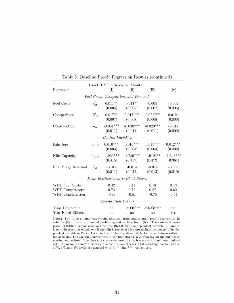
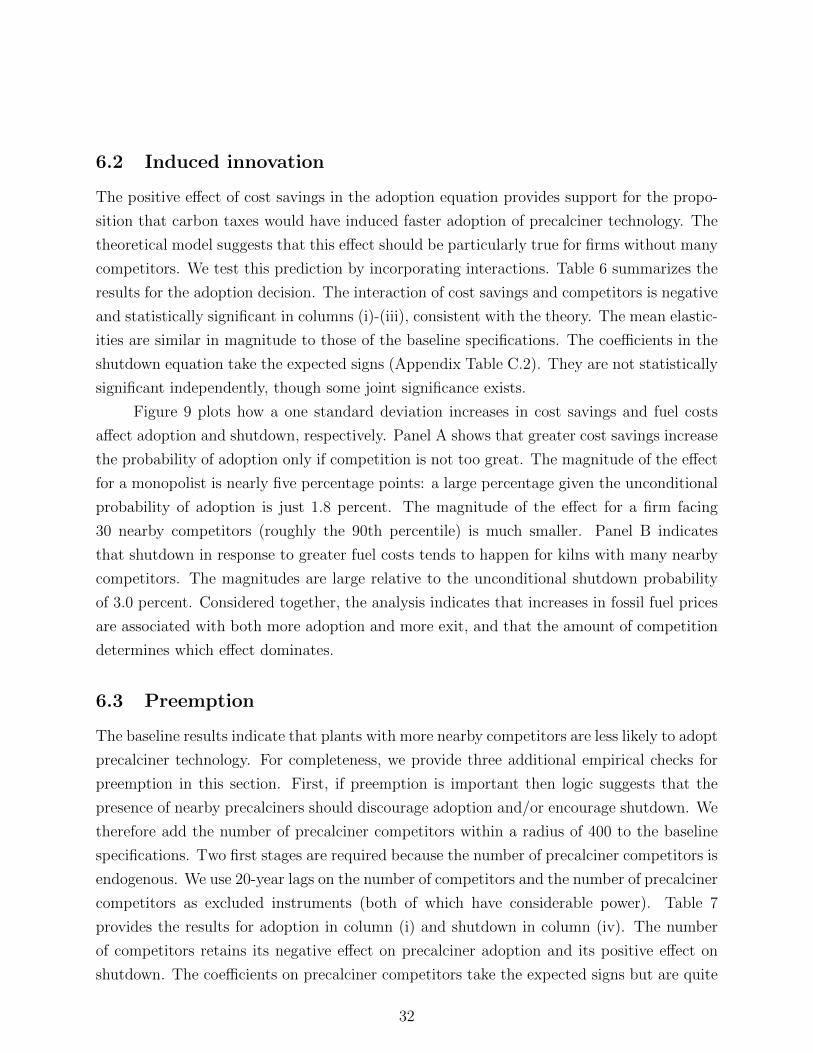
6.2 Induced innovation
The positive effect of cost savings in the adoption equation provides support for the propo-
sition that carbon taxes would have induced faster adoption of precalciner technology. The
theoretical model suggests that this effect should be particularly true for firms without many
competitors. We test this prediction by incorporating interactions. Table 6 summarizes the
results for the adoption decision. The interaction of cost savings and competitors is negative
and statistically significant in columns (i)-(iii), consistent with the theory. The mean elastic-
ities are similar in magnitude to those of the baseline specifications. The coefficients in the
shutdown equation take the expected signs (Appendix Table C.2). They are not statistically
significant independently, though some joint significance exists.
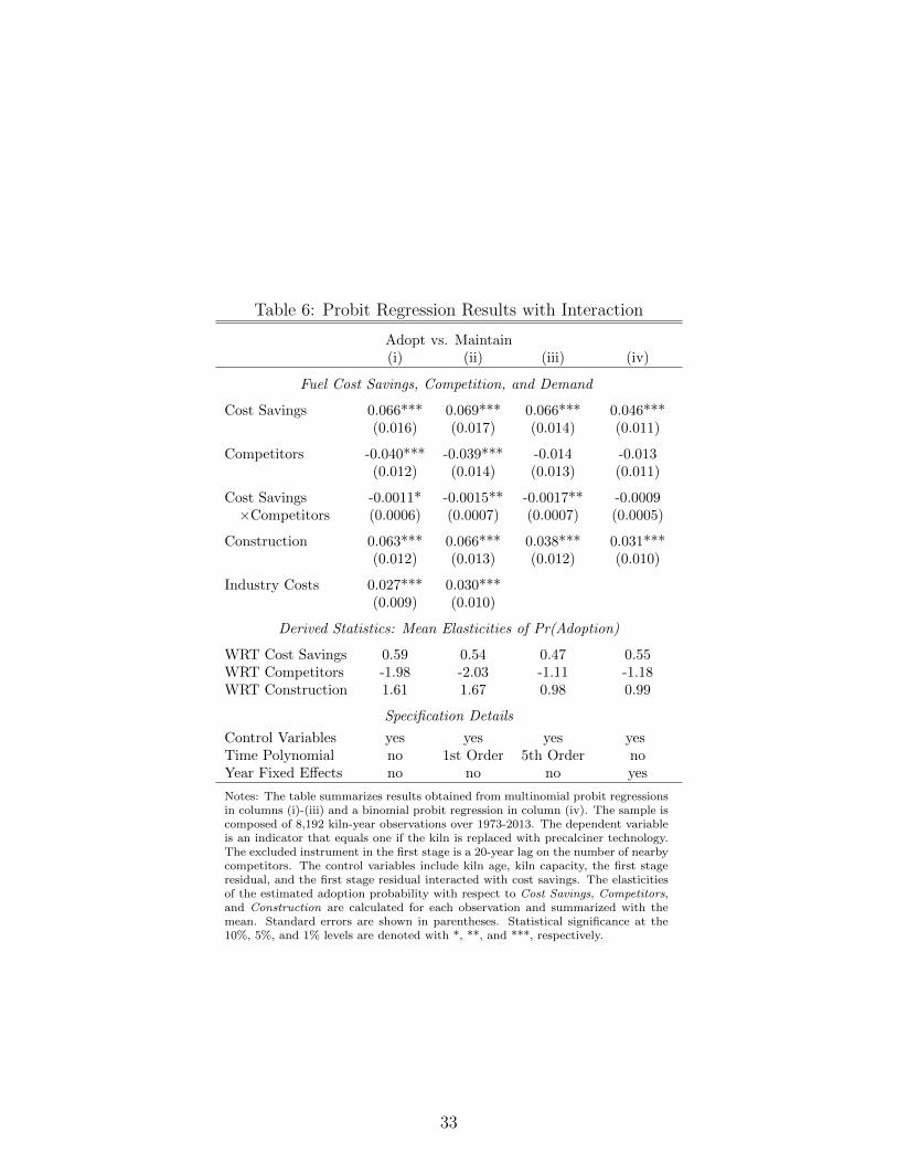
Figure 9 plots how a one standard deviation increases in cost savings and fuel costs
affect adoption and shutdown, respectively. Panel A shows that greater cost savings increase
the probability of adoption only if competition is not too great. The magnitude of the effect
for a monopolist is nearly five percentage points: a large percentage given the unconditional
probability of adoption is just 1.8 percent. The magnitude of the effect for a firm facing
30 nearby competitors (roughly the 90th percentile) is much smaller. Panel B indicates
that shutdown in response to greater fuel costs tends to happen for kilns with many nearby
competitors. The magnitudes are large relative to the unconditional shutdown probability
of 3.0 percent. Considered together, the analysis indicates that increases in fossil fuel prices
are associated with both more adoption and more exit, and that the amount of competition
determines which effect dominates.
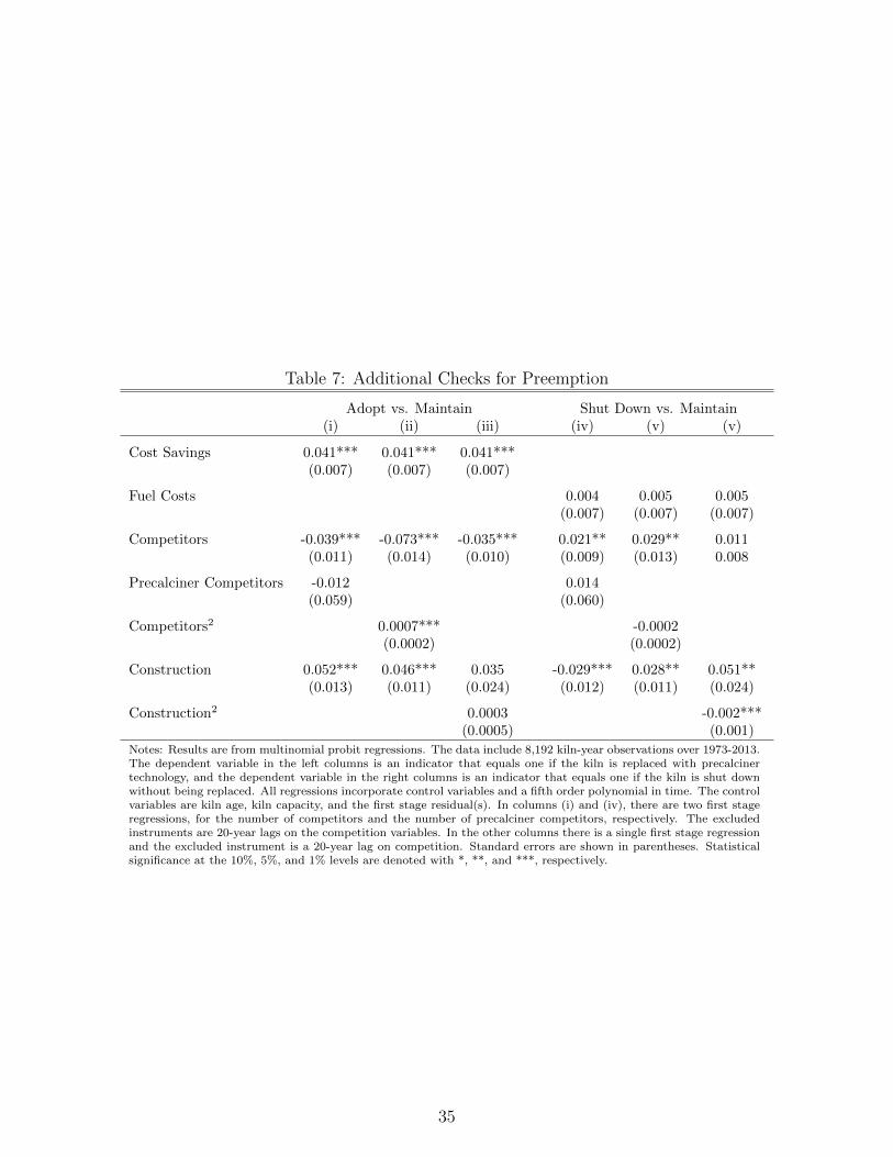
6.3 Preemption
The baseline results indicate that plants with more nearby competitors are less likely to adopt
precalciner technology. For completeness, we provide three additional empirical checks for
preemption in this section. First, if preemption is important then logic suggests that the
presence of nearby precalciners should discourage adoption and/or encourage shutdown. We
therefore add the number of precalciner competitors within a radius of 400 to the baseline
specifications. Two first stages are required because the number of precalciner competitors is
endogenous. We use 20-year lags on the number of competitors and the number of precalciner
competitors as excluded instruments (both of which have considerable power). Table 7
provides the results for adoption in column (i) and shutdown in column (iv). The number
of competitors retains its negative effect on precalciner adoption and its positive effect on
shutdown. The coefficients on precalciner competitors take the expected signs but are quite
32
Table 6: Probit Regression Results with Interaction
Control Variables yes yes yes yesTime Polynomial no 1st Order 5th Order noYear Fixed Effects no no no yes
Notes: The table summarizes results obtained from multinomial probit regressionsin columns (i)-(iii) and a binomial probit regression in column (iv). The sample iscomposed of 8,192 kiln-year observations over 1973-2013. The dependent variableis an indicator that equals one if the kiln is replaced with precalciner technology.The excluded instrument in the first stage is a 20-year lag on the number of nearbycompetitors. The control variables include kiln age, kiln capacity, the first stageresidual, and the first stage residual interacted with cost savings. The elasticitiesof the estimated adoption probability with respect to Cost Savings, Competitors,and Construction are calculated for each observation and summarized with themean. Standard errors are shown in parentheses. Statistical significance at the10%, 5%, and 1% levels are denoted with *, **, and ***, respectively.
33
0
.01
.02
.03
.04
.05
.06
.07
.08
Cha
nge
in P
roba
bilit
y
0 5 10 15 20 25 30 35 40 45 50Competitors
Panel A: Effect of Cost Savings on Adoption
0
.01
.02
.03
.04
0 5 10 15 20 25 30 35 40 45 50Competitors
Panel B: Effect of Fuel Cost on Shutdown
Figure 9: Changes in the Probabilities of Adoption and ShutdownNotes: Panel A plots changes in precalciner adoption probabilities due to a one standard deviation increasein cost savings (which is 6.62). Panel B plots changes in kiln shutdown probabilities due to a one standarddeviation increase in fuel costs (which is 9.63). Both effects are evaluated over the number of nearbycompetitors. Results are based on specification (ii) in Table 6. Other explanatory variables are held at theirrespective means. The shaded regions provide 95% confidence intervals.
imprecisely estimated. Thus, the regression does not provide compelling empirical support
for the hypothesis that early adoption preempts competitors or encourages shutdown.
Second, the theoretical model indicates that if preemption incentives are strong enough
then an inverted-U relationship between competition and adoption arises in the early periods
of industry adoption. If the inverted-U is present, however, it is a short-term phenomenon
because the theoretical model is unambiguous that competition weakly decreases long run
adoption. We test for an inverted-U relationship by allowing the benefits of adoption to have
a quadratic relationship with the competition measure. In estimation, we also incorporate
a quadratic in the estimated first-stage residual. The results are provided in columns (ii)
and (v). The quadratic term is positive in the adoption equation, exactly the opposite of
what would be arise with an inverted-U relationship. We emphasize that the net effect of
the competition regressors is negative in the range of the data, so the results should not be
misinterpreted as implying that a sufficiently high degree of competition increases adoption.
A third approach to testing for preemption is to see whether adoption is most likely for
moderate levels of demand (e.g., Dafny (2005) Ellison and Ellison (2011)). The logic is that
competitors definitely would not adopt with low enough demand and definitely would adopt
with high enough demand, which isolates intermediate ranges of demand as candidates for
34
Table 7: Additional Checks for Preemption
Adopt vs. Maintain Shut Down vs. Maintain(i) (ii) (iii) (iv) (v) (v)
Notes: Results are from multinomial probit regressions. The data include 8,192 kiln-year observations over 1973-2013.The dependent variable in the left columns is an indicator that equals one if the kiln is replaced with precalcinertechnology, and the dependent variable in the right columns is an indicator that equals one if the kiln is shut downwithout being replaced. All regressions incorporate control variables and a fifth order polynomial in time. The controlvariables are kiln age, kiln capacity, and the first stage residual(s). In columns (i) and (iv), there are two first stageregressions, for the number of competitors and the number of precalciner competitors, respectively. The excludedinstruments are 20-year lags on the competition variables. In the other columns there is a single first stage regressionand the excluded instrument is a 20-year lag on competition. Standard errors are shown in parentheses. Statisticalsignificance at the 10%, 5%, and 1% levels are denoted with *, **, and ***, respectively.
35
supporting preemption. We implement by adding a quadratic term in Construction. The
results are shown in columns (iii) and (vi). The coefficient on the quadratic term is positive
in the adoption equation. This result does not support preemption, but the standard error
is large enough that the opposite relationship cannot be ruled out.
6.4 Robustness analysis
The results developed above are robust to alternative choices related to the distribution of
the structural error terms, variable definitions, and the relevant sample period. Regressions
that use the binomial probit, binomial logit, and multinomial logit models return basically
identical results. The linear probability model also returns similar effects in terms of both
magnitude and statistical significance. We also have used a “competing risks” semipara-
metric hazard rate model (Fine and Gray (1999)), in which shutdown is incorporated as an
exogenous event rather than as an endogenous decision driven by particular economic circum-
stances. Results are consistent with the binomial probit. The estimates appear to be driven
by the empirical variation in the data rather than particular distributional assumptions.
Table 8 evaluates robustness with respect to variable definitions and sample periods.
We use binomial probit regressions to estimate the adoption equation. Column (i) adds two
alternative cost savings measures, based on fossil fuel prices five years ahead and behind
the year of the observation. These alternative measures do not predict adoption. Column
(ii) modifies the number of competitors based on a tighter distance radius of 200. This
alternative competition measure does not affect the results much. Column (iii) uses both
the baseline radius (400) and the alternative radius (200), and both variables are found
negative and statistically significant. The total effect of a competitor within a radius of 200
is −0.015 − 0.041 = −0.056. Closer competitors matter more, which is consistent with the
role of transportation costs. Columns (iv) and (v) use subsamples that respectively span
1973-1990 and 1991-2013. The results do not differ substantially.
Table 9 explores the IV strategy. Again we use binomial probit regressions to estimate
the adoption equation. Column (i) excludes the first stage residual. The number of nearby
competitors still has a negative effect but the magnitude is reduced. The direction of this
change is consistent with expectations given the source of bias. Columns (ii)-(iv) respectively
use 5-year, 10-year, and 15-year lags on competition as the excluded instrument, instead of
the 20-year lags used in the baseline specifications. The magnitude of the estimated effect of
nearby competitors is greater if a longer lag is used as an instrument. The mean elasticity of
adoption with respect to competition is −1.37 with the 15-year lag, which is not statistically
36
Table 8: Probit Regressions with Alternative Regressors and Samples
Construction 0.030*** 0.085*** 0.042*** 0.041** 0.032**(0.011) (0.017) (0.009) (0.018) (0.013)
Notes: Results are from binomial probit regressions. The dependent variable is an indicator thatequals one if the kiln is replaced with precalciner technology. The data in columns (i)-(iii) include8,192 kiln-year observations over 1973-2013. The data in column (iv) include 5,149 kiln-yearobservations over 1973-1990, and the data in column (v) include 3,043 kiln-year observationsover 1991-2010. All regressions incorporate control variables and a fifth order polynomial intime. The control variables are kiln age, kiln capacity, and the first stage residual. The excludedinstrument in the first stage is a 20-year lag on the number of nearby competitors. Standarderrors are shown in parentheses. Statistical significance at the 10%, 5%, and 1% levels aredenoted with *, **, and ***, respectively.
37
Table 9: Probit Regression Results with Alternative IVs
Notes: Results are from binomial probit regressions. The dependent variable is anindicator that equals one if the kiln is replaced with precalciner technology. Thedata include 8,192 kiln-year observations over 1973-2013. All regressions incorpo-rate control variables and a fifth order polynomial in time. The control variablesare kiln age, kiln capacity, and the first stage residual. The excluded instrumentin the first stage is a lag on the number of nearby competitors, as described withinthe columns. The elasticities of the estimated adoption probability with respectto Cost Savings, Competitors, and Construction are calculated for each observa-tion and summarized with the mean. Standard errors are shown in parentheses.Statistical significance at the 10%, 5%, and 1% levels are denoted with *, **, and***, respectively.
different from the −1.57 mean elasticity obtained with the comparable baseline specification.
Thus, while the results suggest even longer lags might be required to fully eliminate bias,
the effects of persistence in the error term appear to mostly die out within 15-20 years.
7 Conclusion
Our research explores precalciner adoption in the portland cement industry. The precalciner
kiln reasonably can be characterized as belonging to a broad class of non-drastic, non-
exclusive, and non-divisible cost-reducing technologies. A theoretical analysis of this setting
shows that adoption incentives exhibit a Schumpeterian flair: competition can deprive firms
of the scale necessary to recoup fixed adoption costs. The empirical analysis of firm policy
functions comports with comparative statics of the theoretical model and indicates that
plants with fewer nearby competitions are more likely to adopt precalciner technology.
38
The fundamental argument of Schumpeter (1942) is that market power in capitalist
economies creates conditions under which “the perennial gale of creative destruction” facil-
itates innovation and growth. Thus, it may seem ironic that support for the Schumpeterian
hypothesis is found in the staid industry of portland cement, which has used broadly similar
production technologies for more than a century. On the other hand, three generations of
Schumpeter’s ancestors ran a successful textiles company, at one point installing the first
steam engine in Triesch in modern-day Czech Republic; at least one biographer speculates
this family history contributed to Schumpeter’s interests in entrepreneurship and innovation
McCraw (2007, p. 11). Furthermore, it is precisely the stability of the portland cement indus-
try that makes it amenable to careful empirical analysis. In this sense, our research is similar
to other studies that have found support for Schumpeterian hypotheses in the diffusion of
process innovations (e.g., Hannan and McDowell (1984); Rose and Joskow (1990); Karshenas
and Stoneman (1993); Akhavein, Frame and White (2005); Schmidt-Dengler (2006)).
We conclude with a brief discussion of possible extensions. Our current research focuses
on how and why competition affects firm policies regarding technology adoption. We have
not (yet) examined welfare effects. It also is possible to incorporate entry and exit into the
model. Our early efforts on this front indicate that preemption effects become somewhat
stronger with exit, but that otherwise the comparative statics are unchanged. We have opted
to present the simpler model here. The main advantage to the richer model is that it is more
suitable for structural analyses of industry adjustment paths. Such an undertaking would
require simplifying restrictions on the state space, but if these can be made without too
much loss of realism then useful results could be obtained on a number of subjects, including
the welfare consequences of market-based regulation.
39
References
Abernathy, William J. and James M. Utterback, “Patterns of Industrial Innovation,”
Technology Review, June/July 1978, pp. 41–47.
Acemoglu, Daron, Ufuk Akcigit, Douglas Hanley, and William Kerr, “Transition
to Clean Technology,” Journal of Political Economy, 2016, 124 (1), 52–104.
Aghion, Philippe and Jean Tirole, “The Management of Innovation,” Quarterly Journal
of Economics, 1994, 109, 1185–1209.
and Rachel Griffith, Competition and Growth: Reconciling Theory and Evidence,
The MIT Press, 2005.
, Antoine Dechezlepretre, David Hemous, Ralf Martin, and John Van
Reenen, “Carbon Taxes, Path Dependency and Directed Technical Change: Evidence
from the Auto Industry,” 2012. NBER Working Paper 18596.
, Nicholas Bloom, Richard Blundell, Rachel Griffith, and Peter Howitt,
“Competition and Innovation: An Inverted U-Relationship,” Quarterly Journal of Eco-
nomics, 2005, 120, 701728.
Akhavein, Jalal, W. Scott Frame, and Lawrence J. White, “The Diffusion of Finan-
cial Innovations: An Examination of the Adoption of Small Business Credit Scoring in
Large Banking Organizations,” Journal of Business, 2005, 78 (2), 577–596.
Amemiya, Takesh, “The Estimation of a Simultaneous Equation Generalized Probit
Model,” Econometrica, 1978, 46, 1193–1205.
Arrow, Kenneth J., “Economic Welfare and the Allocation of Resouces for Invention,”
1962. In The Rate and Direction of Inventive Activity: Economic and Social Factors,
ed. J. Neyman, 507-532. Berkeley: University of California Press.
Bajari, P., L. Benkard, and J. Levin, “Estimating Dynamic Models of Imperfect Com-
petition,” Econometrica, 2007, pp. 1331–1370.
Baldwin, William L. and John T. Scott, “Market Structure and Technological Change,”
1987. In Lesourne and Sonnenschein (Eds.), Fundamentals of Pure and Applied Eco-
nomics. Chur, Switzerland, and London: Harwook Academic Publishers.
40
Busse, Meghan R., Christopher R. Knittel, and Florian Zettelmeyer, “Are Con-
sumers Myopic? Evidence from New and Used Car Purchases,” American Economic
Review, 2013, 103 (1), 220–256.
Carbon War Room, “Gigatron Analysis of the Cement Industry,” 2011.
Chicu, Mark, “Dynamic Investment and Deterrence in the U.S. Cement Industry,” 2012.
Job Market Paper, Northwestern University.
Cohen, Wesley M., “Empirical Studies of Innovative Activity,” 1995. In Stoneman, P.
(Ed.), Handbook of the Economics of Innovation and Technical Change. Oxford: Basil
Blackwell.
, “Fifty Years of Empirical Studies of Innovative Activity and Performance,” 2010. In
Arrow, K.J. and Intriligator, M.D. (eds), Handbook of the Economics of Innovation,
Volume 01. Elsevier.
and Richard C. Levin, “Empirical Studies of Innovation and Market Structure,”
1989. In Schmalensee, R. and Willig, R. (Eds.), Handbook of Industrial Organization.
Amsterdam: North-Holland.
Dafny, Leemore, “Games that Hospitals Play: Entry Deterrence in Hospital Procedure
Time Polynomial no 1st Order 5th Order noYear Fixed Effects no no no yes
Notes: The table summarizes results obtained from multinomial probit regres-sions in columns (i)-(iii) and a binomial probit regressions in column (iv). Thesample is comprised of 8,192 kiln-year observations over 1973-2013. The ex-cluded instrument in the first stage is a 20-year lag on the number of nearbycompetitors. The elasticities are calculated for each observation and summa-rized with the mean. Standard errors are shown in parentheses. Statisticalsignificance at the 10%, 5%, and 1% levels are denoted with *, **, and ***,respectively.