Slide 1

Finish SearchJim Little

UBC CS 322 – Search 7September 24, 2014

Textbook §3.6

Slide 2

Lecture Overview• Finish MBA*• Pruning Cycles and Repeated

states Examples• Dynamic Programming• Search Recap

Slide 3

Heuristic value by look ahead

Slide 4

Memory-bounded A*

• Iterative deepening A* and B & B use a tiny amount of memory

• what if we've got more memory to use?• keep as much of the fringe in memory as we can• if we have to delete something:

• delete the worst paths ( )• ``back them up'' to a common ancestor

p

pnp1

highest f

Slide 5

MBA*: Compute New h(p)

Slide 6

Lecture Overview• Finish MBA*• Interlude: State Space/Search

Graphs• Pruning Cycles and Repeated

states Examples• Dynamic Programming• Search Recap

Clarification: state space graph vs search tree

7

k c

b z

h

akb kc

kbz

d

fkbza kbzd

kch

k

State space graph.

If there are no cycles, the two look the same

Search tree.Nodes in this tree correspond to paths in the state space graph

kchfy

4 5

6 7 8

Clarification: state space graph vs search tree

8

k c

b z

h

akb kc

kbz

d

fkbza kbzd

kch

k

State space graph.

Search tree.

kchf

4 5

6 7 8

8

The numbers in the search tree’s nodes mean?Node’s name

Order in which a search algo. (here: BFS) expands nodes

Clarification: state space graph vs search tree

9

k c

b z

h

akb kc

kbk kbz

d

fkbkb kbkc

kbza kbzd

kch

kchf

kckb

kckc

kck

k

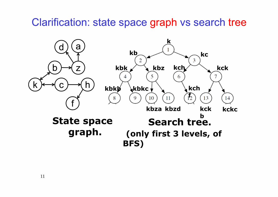
State space graph.

Search tree. (only first 3 levels, of

BFS)• If there are cycles, the two look very different

Clarification: state space graph vs search tree

10

k c

b z

h

akb kc

kbk kbz

d

fkbkb kbkc

kbza kbzd

kch

kchf

kckb

kckc

kck

k

State space graph.

Search tree. (only first 3 levels, of

BFS)

Clarification: state space graph vs search tree

11

k c

b z

h

akb kc

kbk kbz

d

fkbkb kbkc

kbza kbzd

kch

kchf

kckb

kckc

kck

k

State space graph.

Search tree. (only first 3 levels, of

BFS)

Clarification: state space graph vs search tree

12

k c

b z

h

akb kc

kbk kbz

d

zkbkb kbkc

kbza kbzd

kch

kchz

kckb

kckc

kck

k

State space graph.

May contain cycles!

Search tree.Nodes in this tree correspond to paths in the state space graph

(if multiple start nodes: forest)

Cannot contain cycles!

Clarification: state space graph vs search tree

13

k c

b z

h

akb kc

kbk kbz

d

zkbkb kbkc

kbza kbzd

kch

kchz

kckb

kckc

kck

k

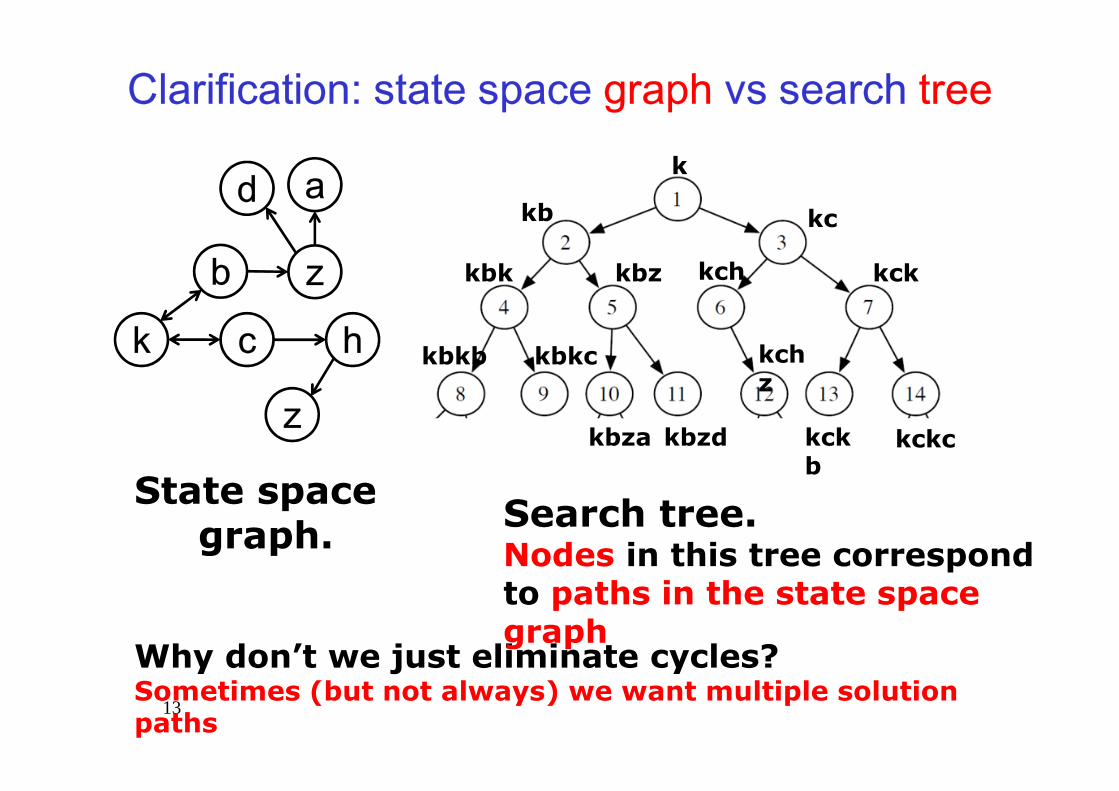
State space graph.

Why don’t we just eliminate cycles?Sometimes (but not always) we want multiple solution paths

Search tree.Nodes in this tree correspond to paths in the state space graph

Slide 14

Lecture Overview• Finish MBA*• Pruning Cycles and Repeated

states Examples• Dynamic Programming• Search Recap

Slide 15

Multiple-Path Pruning & Optimal Solutions

Problem: what if a subsequent path to n is shorter than the first path to n ?

• You can remove all paths from the frontier that use the longer path. (as these can’t be optimal)

Slide 16

Multiple-Path Pruning & Optimal Solutions

Problem: what if a subsequent path to n is shorter than the first path to n ?

• You can change the initial segment of the paths on the frontier to use the shorter path.

Pruning Cycles

Slide 17

Repeated States

Example

Slide 18

Lecture Overview• Finish MBA*• Pruning Cycles and Repeated

states Examples• Dynamic Programming• Search Recap

Dynamic Programming• Idea: for statically stored graphs, build a table of dist(n):

• The actual distance of the shortest path from node n to a goal g

• This is the perfect

• dist(g) = 0• dist(z) = 1• dist(c) = 3• dist(b) = 4• dist(k) = ?

• dist(h) = ?

• How could we implement that?

k c

b h

g

z

2

3

1

2

4

1

7 ∞6

7 ∞6

heuristiccostf function

Slide 19

Slide 20

This can be built backwards from the goal:

Dynamic Programming

( )

+=∈ otherwisemdistmn

ngoalisifndist

Amn )(),(costmin

),(_0)(

,

a

b

cg

2

31

3

g

b

c

a

2d

1

2

����(�)

= �� 2 + 0 = 2

= �� 3 + 0 = 3

= �� 3 + 3 , (1 + 2) = 3

0m

Slide 21

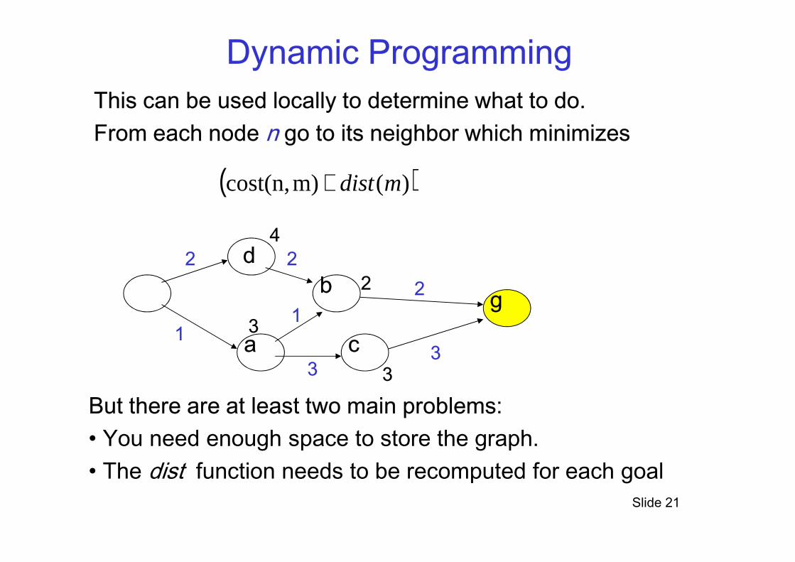
But there are at least two main problems:• You need enough space to store the graph.• The dist function needs to be recomputed for each goal

Dynamic ProgrammingThis can be used locally to determine what to do.From each node n go to its neighbor which minimizes

a

b

c

g2

3

4

3

d

3

21

3

( ))(m)cost(n, mdist+

2

1

2

Slide 22

Lecture Overview• Finish MBA*• Pruning Cycles and Repeated

states Examples• Dynamic Programming• Search Recap

Slide 23

Recap SearchSelection Complete Optimal Time Space

DFS LIFO N N O(bm) O(mb)BFS FIFO Y Y O(bm) O(bm)

IDS(C) LIFO Y Y O(bm) O(mb)

LCFS min cost Y Y O(bm) O(bm)

BFS min h N N O(bm) O(bm)A* min f Y Y O(bm) O(bm)

B&B LIFO + pruning

N Y O(bm) O(mb)

IDA* LIFO Y Y O(bm) O(mb)

MBA* min f N Y O(bm) O(bm)

Slide 24

Recap Search (some qualifications)Complete Optimal Time Space

DFS N N O(bm) O(mb)BFS Y Y O(bm) O(bm)

IDS(C) Y Y O(bm) O(mb)

LCFS Y Y ? O(bm) O(bm)

BFS N N O(bm) O(bm)A* Y Y ? O(bm) O(bm)

B&B N Y ? O(bm) O(mb)

IDA* Y Y O(bm) O(mb)

MBA* N Y O(bm) O(bm)

C>0

h admiss.

no inf path

Slide 25

Search in PracticeComplete Optimal Time Space

DFS N N O(bm) O(mb)BFS Y Y O(bm) O(bm)

IDS(C) Y Y O(bm) O(mb)

LCFS Y Y O(bm) O(bm)

BFS N N O(bm) O(bm)A* Y Y O(bm) O(bm)

B&B N Y O(bm) O(mb)

IDA* Y Y O(bm) O(mb)

MBA* N Y O(bm) O(bm)

BDS Y Y O(bm/2) O(bm/2)

Slide 26

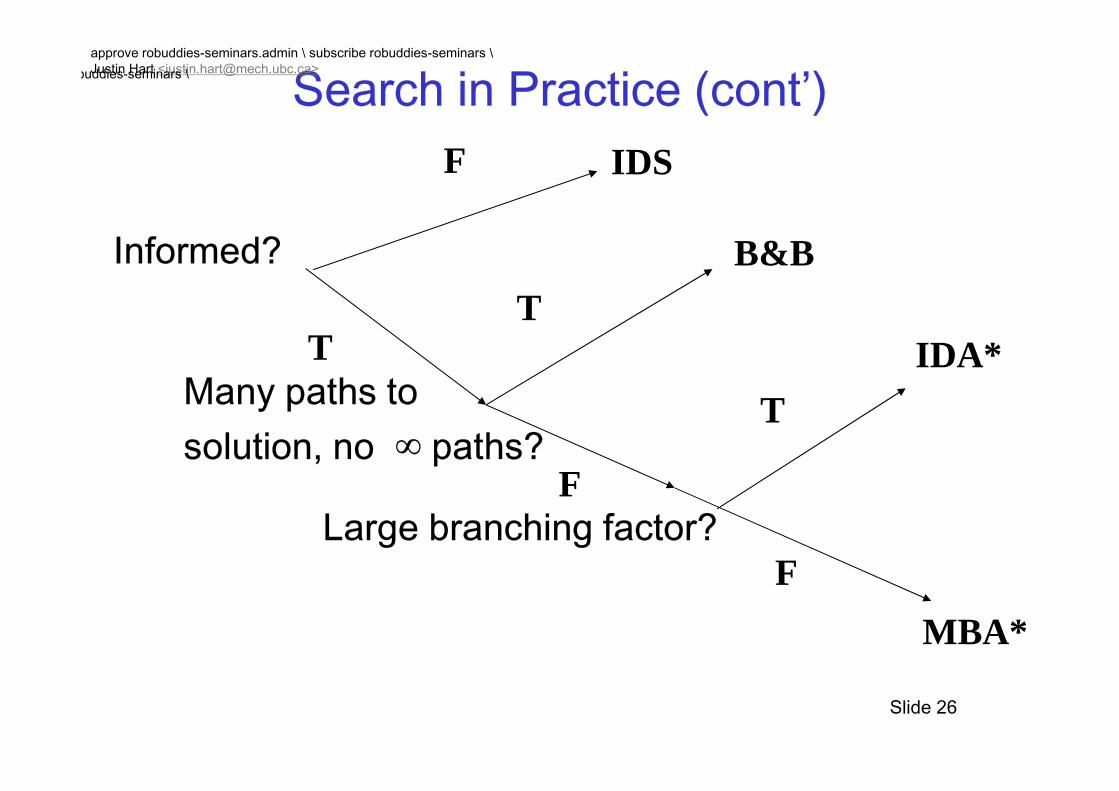
Search in Practice (cont’)

Many paths to solution, no ∞ paths?

Informed?

Large branching factor?

F

T

approve robuddies-seminars.admin \ subscribe robuddies-seminars \Justin Hart <justin.hart@mech.ubc.ca>

T

subscribe robuddies-seminars \

T

F

F

IDS

B&B

MBA*

IDA*

Slide 27

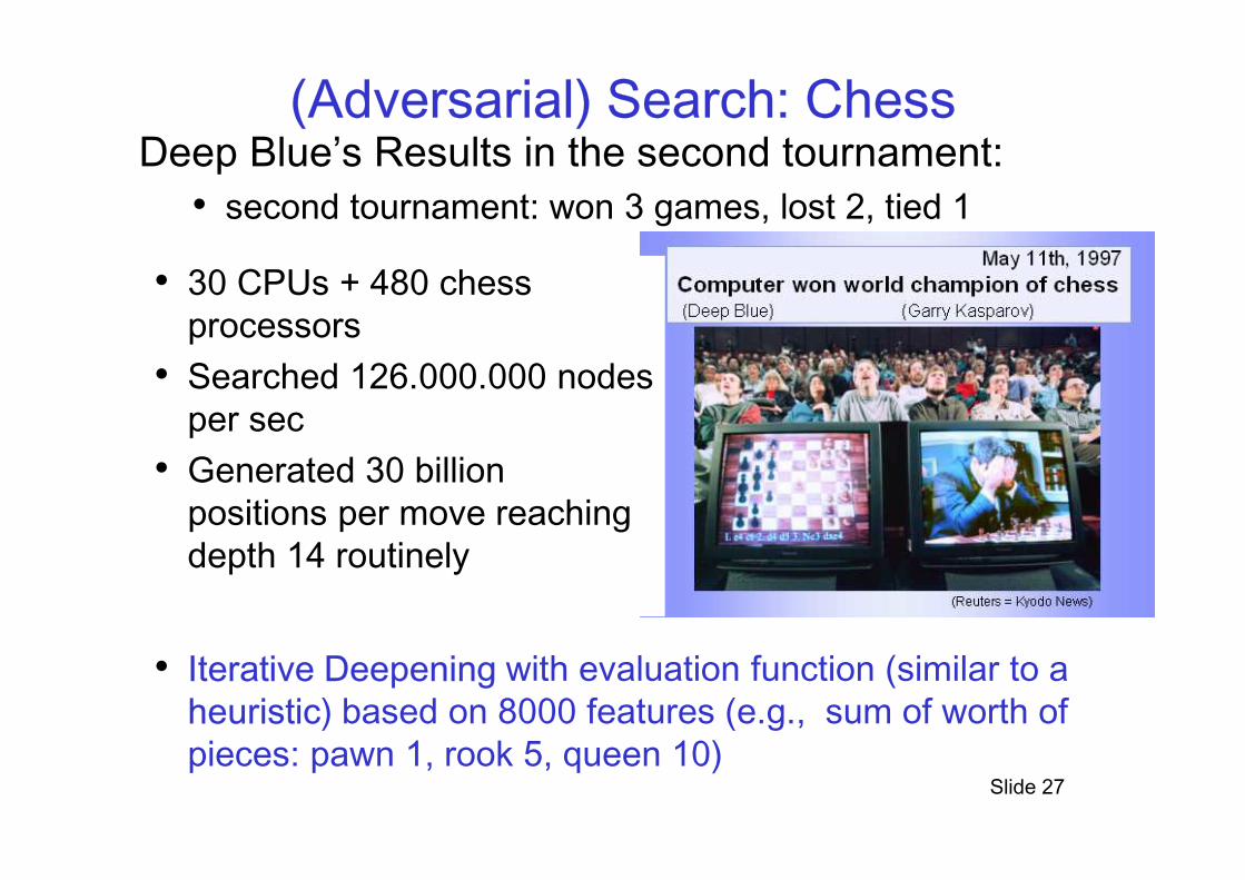
(Adversarial) Search: ChessDeep Blue’s Results in the second tournament:

• second tournament: won 3 games, lost 2, tied 1

• 30 CPUs + 480 chess processors

• Searched 126.000.000 nodes per sec

• Generated 30 billion positions per move reaching depth 14 routinely

• Iterative Deepening with evaluation function (similar to a heuristic) based on 8000 features (e.g., sum of worth of pieces: pawn 1, rook 5, queen 10)

Slide 28

Modules we'll cover in this course: R&RsysEnvironment

Problem

Query

Planning

Deterministic Stochastic

Search

Arc Consistency

Search

SearchValue Iteration

Var. Elimination

Constraint Satisfaction

Logics

STRIPS

Belief Nets

Vars + Constraints

Decision Nets

Markov ProcessesVar. Elimination

Static

Sequential

RepresentationReasoningTechnique

Slide 29

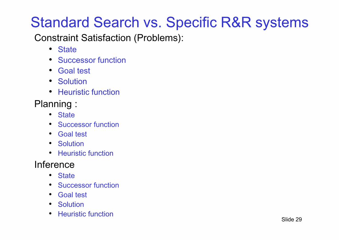
Standard Search vs. Specific R&R systemsConstraint Satisfaction (Problems):

• State• Successor function• Goal test• Solution• Heuristic function

Planning : • State• Successor function• Goal test• Solution• Heuristic function

Inference• State• Successor function• Goal test• Solution• Heuristic function

Slide 30

Next class

Start Constraint Satisfaction Problems (CSPs)Textbook 4.1-4.3