125
Finite Difference Methods for Ordinary and Partial Differential Equations OT98_LevequeFM2.qxp 6/4/2007 10:20 AM Page 1
Finite Difference Methodsfor Ordinary and PartialDifferential Equations
OT98_LevequeFM2.qxp 6/4/2007 10:20 AM Page 1

OT98_LevequeFM2.qxp 6/4/2007 10:20 AM Page 2
Finite Difference Methodsfor Ordinary and PartialDifferential EquationsSteady-State and Time-Dependent Problems
Randall J. LeVequeUniversity of WashingtonSeattle, Washington
Society for Industrial and Applied Mathematics • Philadelphia
OT98_LevequeFM2.qxp 6/4/2007 10:20 AM Page 3

Copyright © 2007 by the Society for Industrial and Applied Mathematics.
10 9 8 7 6 5 4 3 2 1
All rights reserved. Printed in the United States of America. No part of this book may bereproduced, stored, or transmitted in any manner without the written permission of the publisher. For information, write to the Society for Industrial and Applied Mathematics, 3600University City Science Center, Philadelphia, PA 19104-2688.
Trademarked names may be used in this book without the inclusion of a trademark symbol.These names are used in an editorial context only; no infringement of trademark is intended.
MATLAB is a registered trademark of The MathWorks, Inc. For MATLAB product information,please contact The MathWorks, Inc., 3 Apple Hill Drive, Natick, MA 01760-2098 USA, 508-647-7000, Fax: 508-647-7101, [email protected], www.mathworks.com.
Library of Congress Cataloging-in-Publication Data
LeVeque, Randall J., 1955-Finite difference methods for ordinary and partial differential equations : steady-state and time-dependent problems / Randall J. LeVeque.
p.cm.Includes bibliographical references and index.ISBN 978-0-898716-29-0 (alk. paper)
1. Finite differences. 2. Differential equations. I. Title.
QA431.L548 2007515’.35—dc22 2007061732
Partial royalties from the sale of this book are placed in a fund to help studentsattend SIAM meetings and other SIAM-related activities. This fund is administeredby SIAM, and qualified individuals are encouraged to write directly to SIAM for guidelines.
is a registered trademark.
OT98_LevequeFM2.qxp 6/4/2007 10:20 AM Page 4

To my family,Loyce, Ben, Bill, and Ann
OT98_LevequeFM2.qxp 6/4/2007 10:20 AM Page 5

“rjlfdm”2007/6/1page vii✐
✐✐
✐
✐✐
✐✐
Contents
Preface xiii
I Boundary Value Problems and Iterative Methods 1
1 Finite Difference Approximations 31.1 Truncation errors . . . . . . . . . . . . . . . . . . . . . . . . . . . . . 51.2 Deriving finite difference approximations . . . . . . . . . . . . . . . . 71.3 Second order derivatives . . . . . . . . . . . . . . . . . . . . . . . . . 81.4 Higher order derivatives . . . . . . . . . . . . . . . . . . . . . . . . . 91.5 A general approach to deriving the coefficients . . . . . . . . . . . . . 10
2 Steady States and Boundary Value Problems 132.1 The heat equation . . . . . . . . . . . . . . . . . . . . . . . . . . . . 132.2 Boundary conditions . . . . . . . . . . . . . . . . . . . . . . . . . . . 142.3 The steady-state problem . . . . . . . . . . . . . . . . . . . . . . . . 142.4 A simple finite difference method . . . . . . . . . . . . . . . . . . . . 152.5 Local truncation error . . . . . . . . . . . . . . . . . . . . . . . . . . 172.6 Global error . . . . . . . . . . . . . . . . . . . . . . . . . . . . . . . 182.7 Stability . . . . . . . . . . . . . . . . . . . . . . . . . . . . . . . . . 182.8 Consistency . . . . . . . . . . . . . . . . . . . . . . . . . . . . . . . 192.9 Convergence . . . . . . . . . . . . . . . . . . . . . . . . . . . . . . . 192.10 Stability in the 2-norm . . . . . . . . . . . . . . . . . . . . . . . . . . 202.11 Green’s functions and max-norm stability . . . . . . . . . . . . . . . . 222.12 Neumann boundary conditions . . . . . . . . . . . . . . . . . . . . . 292.13 Existence and uniqueness . . . . . . . . . . . . . . . . . . . . . . . . 322.14 Ordering the unknowns and equations . . . . . . . . . . . . . . . . . . 342.15 A general linear second order equation . . . . . . . . . . . . . . . . . 352.16 Nonlinear equations . . . . . . . . . . . . . . . . . . . . . . . . . . . 37
2.16.1 Discretization of the nonlinear boundary value problem . 382.16.2 Nonuniqueness . . . . . . . . . . . . . . . . . . . . . . . 402.16.3 Accuracy on nonlinear equations . . . . . . . . . . . . . 41
2.17 Singular perturbations and boundary layers . . . . . . . . . . . . . . . 432.17.1 Interior layers . . . . . . . . . . . . . . . . . . . . . . . 46
vii

“rjlfdm”2007/6/1page viii✐
✐✐
✐
✐✐
✐✐
viii Contents
2.18 Nonuniform grids . . . . . . . . . . . . . . . . . . . . . . . . . . . . 492.18.1 Adaptive mesh selection . . . . . . . . . . . . . . . . . . 51
2.19 Continuation methods . . . . . . . . . . . . . . . . . . . . . . . . . . 522.20 Higher order methods . . . . . . . . . . . . . . . . . . . . . . . . . . 52
2.20.1 Fourth order differencing . . . . . . . . . . . . . . . . . 522.20.2 Extrapolation methods . . . . . . . . . . . . . . . . . . . 532.20.3 Deferred corrections . . . . . . . . . . . . . . . . . . . . 54
2.21 Spectral methods . . . . . . . . . . . . . . . . . . . . . . . . . . . . . 55
3 Elliptic Equations 593.1 Steady-state heat conduction . . . . . . . . . . . . . . . . . . . . . . 593.2 The 5-point stencil for the Laplacian . . . . . . . . . . . . . . . . . . 603.3 Ordering the unknowns and equations . . . . . . . . . . . . . . . . . . 613.4 Accuracy and stability . . . . . . . . . . . . . . . . . . . . . . . . . . 633.5 The 9-point Laplacian . . . . . . . . . . . . . . . . . . . . . . . . . . 643.6 Other elliptic equations . . . . . . . . . . . . . . . . . . . . . . . . . 663.7 Solving the linear system . . . . . . . . . . . . . . . . . . . . . . . . 66
3.7.1 Sparse storage in MATLAB . . . . . . . . . . . . . . . . 68
4 Iterative Methods for Sparse Linear Systems 694.1 Jacobi and Gauss–Seidel . . . . . . . . . . . . . . . . . . . . . . . . . 694.2 Analysis of matrix splitting methods . . . . . . . . . . . . . . . . . . 71
4.2.1 Rate of convergence . . . . . . . . . . . . . . . . . . . . 744.2.2 Successive overrelaxation . . . . . . . . . . . . . . . . . 76
4.3 Descent methods and conjugate gradients . . . . . . . . . . . . . . . . 784.3.1 The method of steepest descent . . . . . . . . . . . . . . 794.3.2 The A-conjugate search direction . . . . . . . . . . . . . 834.3.3 The conjugate-gradient algorithm . . . . . . . . . . . . . 864.3.4 Convergence of conjugate gradient . . . . . . . . . . . . 884.3.5 Preconditioners . . . . . . . . . . . . . . . . . . . . . . 934.3.6 Incomplete Cholesky and ILU preconditioners . . . . . . 96
4.4 The Arnoldi process and GMRES algorithm . . . . . . . . . . . . . . 964.4.1 Krylov methods based on three term recurrences . . . . . 994.4.2 Other applications of Arnoldi . . . . . . . . . . . . . . . 100
4.5 Newton–Krylov methods for nonlinear problems . . . . . . . . . . . . 1014.6 Multigrid methods . . . . . . . . . . . . . . . . . . . . . . . . . . . . 103
4.6.1 Slow convergence of Jacobi . . . . . . . . . . . . . . . . 1034.6.2 The multigrid approach . . . . . . . . . . . . . . . . . . 106
II Initial Value Problems 111
5 The Initial Value Problem for Ordinary Differential Equations 1135.1 Linear ordinary differential equations . . . . . . . . . . . . . . . . . . 114
5.1.1 Duhamel’s principle . . . . . . . . . . . . . . . . . . . . 1155.2 Lipschitz continuity . . . . . . . . . . . . . . . . . . . . . . . . . . . 116
“rjlfdm”2007/6/1page ix✐
✐✐
✐
✐✐
✐✐
Contents ix
5.2.1 Existence and uniqueness of solutions . . . . . . . . . . . 1165.2.2 Systems of equations . . . . . . . . . . . . . . . . . . . 1175.2.3 Significance of the Lipschitz constant . . . . . . . . . . . 1185.2.4 Limitations . . . . . . . . . . . . . . . . . . . . . . . . . 119
5.3 Some basic numerical methods . . . . . . . . . . . . . . . . . . . . . 1205.4 Truncation errors . . . . . . . . . . . . . . . . . . . . . . . . . . . . . 1215.5 One-step errors . . . . . . . . . . . . . . . . . . . . . . . . . . . . . . 1225.6 Taylor series methods . . . . . . . . . . . . . . . . . . . . . . . . . . 1235.7 Runge–Kutta methods . . . . . . . . . . . . . . . . . . . . . . . . . . 124
5.7.1 Embedded methods and error estimation . . . . . . . . . 1285.8 One-step versus multistep methods . . . . . . . . . . . . . . . . . . . 1305.9 Linear multistep methods . . . . . . . . . . . . . . . . . . . . . . . . 131
5.9.1 Local truncation error . . . . . . . . . . . . . . . . . . . 1325.9.2 Characteristic polynomials . . . . . . . . . . . . . . . . . 1335.9.3 Starting values . . . . . . . . . . . . . . . . . . . . . . . 1345.9.4 Predictor-corrector methods . . . . . . . . . . . . . . . . 135
6 Zero-Stability and Convergence for Initial Value Problems 1376.1 Convergence . . . . . . . . . . . . . . . . . . . . . . . . . . . . . . . 1376.2 The test problem . . . . . . . . . . . . . . . . . . . . . . . . . . . . . 1386.3 One-step methods . . . . . . . . . . . . . . . . . . . . . . . . . . . . 138
6.3.1 Euler’s method on linear problems . . . . . . . . . . . . 1386.3.2 Relation to stability for boundary value problems . . . . . 1406.3.3 Euler’s method on nonlinear problems . . . . . . . . . . 1416.3.4 General one-step methods . . . . . . . . . . . . . . . . . 142
6.4 Zero-stability of linear multistep methods . . . . . . . . . . . . . . . . 1436.4.1 Solving linear difference equations . . . . . . . . . . . . 144
7 Absolute Stability for Ordinary Differential Equations 1497.1 Unstable computations with a zero-stable method . . . . . . . . . . . 1497.2 Absolute stability . . . . . . . . . . . . . . . . . . . . . . . . . . . . 1517.3 Stability regions for linear multistep methods . . . . . . . . . . . . . . 1537.4 Systems of ordinary differential equations . . . . . . . . . . . . . . . 156
7.4.1 Chemical kinetics . . . . . . . . . . . . . . . . . . . . . 1577.4.2 Linear systems . . . . . . . . . . . . . . . . . . . . . . . 1587.4.3 Nonlinear systems . . . . . . . . . . . . . . . . . . . . . 160
7.5 Practical choice of step size . . . . . . . . . . . . . . . . . . . . . . . 1617.6 Plotting stability regions . . . . . . . . . . . . . . . . . . . . . . . . . 162
7.6.1 The boundary locus method for linear multistep methods . 1627.6.2 Plotting stability regions of one-step methods . . . . . . . 163
7.7 Relative stability regions and order stars . . . . . . . . . . . . . . . . 164
8 Stiff Ordinary Differential Equations 1678.1 Numerical difficulties . . . . . . . . . . . . . . . . . . . . . . . . . . 1688.2 Characterizations of stiffness . . . . . . . . . . . . . . . . . . . . . . 1698.3 Numerical methods for stiff problems . . . . . . . . . . . . . . . . . . 170

“rjlfdm”2007/6/1page x✐
✐✐
✐
✐✐
✐✐
x Contents
8.3.1 A-stability and A(˛)-stability . . . . . . . . . . . . . . . 1718.3.2 L-stability . . . . . . . . . . . . . . . . . . . . . . . . . 171
8.4 BDF methods . . . . . . . . . . . . . . . . . . . . . . . . . . . . . . 1738.5 The TR-BDF2 method . . . . . . . . . . . . . . . . . . . . . . . . . . 1758.6 Runge–Kutta–Chebyshev explicit methods . . . . . . . . . . . . . . . 175
9 Diffusion Equations and Parabolic Problems 1819.1 Local truncation errors and order of accuracy . . . . . . . . . . . . . . 1839.2 Method of lines discretizations . . . . . . . . . . . . . . . . . . . . . 1849.3 Stability theory . . . . . . . . . . . . . . . . . . . . . . . . . . . . . . 1869.4 Stiffness of the heat equation . . . . . . . . . . . . . . . . . . . . . . 1869.5 Convergence . . . . . . . . . . . . . . . . . . . . . . . . . . . . . . . 189
9.5.1 PDE versus ODE stability theory . . . . . . . . . . . . . 1919.6 Von Neumann analysis . . . . . . . . . . . . . . . . . . . . . . . . . 1929.7 Multidimensional problems . . . . . . . . . . . . . . . . . . . . . . . 1959.8 The locally one-dimensional method . . . . . . . . . . . . . . . . . . 197
9.8.1 Boundary conditions . . . . . . . . . . . . . . . . . . . . 1989.8.2 The alternating direction implicit method . . . . . . . . . 199
9.9 Other discretizations . . . . . . . . . . . . . . . . . . . . . . . . . . . 200
10 Advection Equations and Hyperbolic Systems 20110.1 Advection . . . . . . . . . . . . . . . . . . . . . . . . . . . . . . . . 20110.2 Method of lines discretization . . . . . . . . . . . . . . . . . . . . . . 203
10.2.1 Forward Euler time discretization . . . . . . . . . . . . . 20410.2.2 Leapfrog . . . . . . . . . . . . . . . . . . . . . . . . . . 20510.2.3 Lax–Friedrichs . . . . . . . . . . . . . . . . . . . . . . . 206
10.3 The Lax–Wendroff method . . . . . . . . . . . . . . . . . . . . . . . 20710.3.1 Stability analysis . . . . . . . . . . . . . . . . . . . . . . 209
10.4 Upwind methods . . . . . . . . . . . . . . . . . . . . . . . . . . . . . 21010.4.1 Stability analysis . . . . . . . . . . . . . . . . . . . . . . 21110.4.2 The Beam–Warming method . . . . . . . . . . . . . . . 212
10.5 Von Neumann analysis . . . . . . . . . . . . . . . . . . . . . . . . . 21210.6 Characteristic tracing and interpolation . . . . . . . . . . . . . . . . . 21410.7 The Courant–Friedrichs–Lewy condition . . . . . . . . . . . . . . . . 21510.8 Some numerical results . . . . . . . . . . . . . . . . . . . . . . . . . 21810.9 Modified equations . . . . . . . . . . . . . . . . . . . . . . . . . . . 21810.10 Hyperbolic systems . . . . . . . . . . . . . . . . . . . . . . . . . . . 224
10.10.1 Characteristic variables . . . . . . . . . . . . . . . . . . 22410.11 Numerical methods for hyperbolic systems . . . . . . . . . . . . . . . 22510.12 Initial boundary value problems . . . . . . . . . . . . . . . . . . . . . 226
10.12.1 Analysis of upwind on the initial boundary value problem 22610.12.2 Outflow boundary conditions . . . . . . . . . . . . . . . 228
10.13 Other discretizations . . . . . . . . . . . . . . . . . . . . . . . . . . . 230
11 Mixed Equations 23311.1 Some examples . . . . . . . . . . . . . . . . . . . . . . . . . . . . . 233
“rjlfdm”2007/6/1page xi✐
✐✐
✐
✐✐
✐✐
Contents xi
11.2 Fully coupled method of lines . . . . . . . . . . . . . . . . . . . . . . 23511.3 Fully coupled Taylor series methods . . . . . . . . . . . . . . . . . . 23611.4 Fractional step methods . . . . . . . . . . . . . . . . . . . . . . . . . 23711.5 Implicit-explicit methods . . . . . . . . . . . . . . . . . . . . . . . . 23911.6 Exponential time differencing methods . . . . . . . . . . . . . . . . . 240
11.6.1 Implementing exponential time differencing methods . . 241
III Appendices 243
A Measuring Errors 245A.1 Errors in a scalar value . . . . . . . . . . . . . . . . . . . . . . . . . . 245
A.1.1 Absolute error . . . . . . . . . . . . . . . . . . . . . . . 245A.1.2 Relative error . . . . . . . . . . . . . . . . . . . . . . . . 246
A.2 “Big-oh” and “little-oh” notation . . . . . . . . . . . . . . . . . . . . 247A.3 Errors in vectors . . . . . . . . . . . . . . . . . . . . . . . . . . . . . 248
A.3.1 Norm equivalence . . . . . . . . . . . . . . . . . . . . . 249A.3.2 Matrix norms . . . . . . . . . . . . . . . . . . . . . . . . 250
A.4 Errors in functions . . . . . . . . . . . . . . . . . . . . . . . . . . . . 250A.5 Errors in grid functions . . . . . . . . . . . . . . . . . . . . . . . . . 251
A.5.1 Norm equivalence . . . . . . . . . . . . . . . . . . . . . 252A.6 Estimating errors in numerical solutions . . . . . . . . . . . . . . . . 254
A.6.1 Estimates from the true solution . . . . . . . . . . . . . . 255A.6.2 Estimates from a fine-grid solution . . . . . . . . . . . . 256A.6.3 Estimates from coarser solutions . . . . . . . . . . . . . 256
B Polynomial Interpolation and Orthogonal Polynomials 259B.1 The general interpolation problem . . . . . . . . . . . . . . . . . . . . 259B.2 Polynomial interpolation . . . . . . . . . . . . . . . . . . . . . . . . 260
B.2.1 Monomial basis . . . . . . . . . . . . . . . . . . . . . . 260B.2.2 Lagrange basis . . . . . . . . . . . . . . . . . . . . . . . 260B.2.3 Newton form . . . . . . . . . . . . . . . . . . . . . . . . 260B.2.4 Error in polynomial interpolation . . . . . . . . . . . . . 262
B.3 Orthogonal polynomials . . . . . . . . . . . . . . . . . . . . . . . . . 262B.3.1 Legendre polynomials . . . . . . . . . . . . . . . . . . . 264B.3.2 Chebyshev polynomials . . . . . . . . . . . . . . . . . . 265
C Eigenvalues and Inner-Product Norms 269C.1 Similarity transformations . . . . . . . . . . . . . . . . . . . . . . . . 270C.2 Diagonalizable matrices . . . . . . . . . . . . . . . . . . . . . . . . . 271C.3 The Jordan canonical form . . . . . . . . . . . . . . . . . . . . . . . 271C.4 Symmetric and Hermitian matrices . . . . . . . . . . . . . . . . . . . 273C.5 Skew-symmetric and skew-Hermitian matrices . . . . . . . . . . . . . 274C.6 Normal matrices . . . . . . . . . . . . . . . . . . . . . . . . . . . . . 274C.7 Toeplitz and circulant matrices . . . . . . . . . . . . . . . . . . . . . 275C.8 The Gershgorin theorem . . . . . . . . . . . . . . . . . . . . . . . . . 277
“rjlfdm”2007/6/1page xii✐
✐✐
✐
✐✐
✐✐
xii Contents
C.9 Inner-product norms . . . . . . . . . . . . . . . . . . . . . . . . . . . 279C.10 Other inner-product norms . . . . . . . . . . . . . . . . . . . . . . . 281
D Matrix Powers and Exponentials 285D.1 The resolvent . . . . . . . . . . . . . . . . . . . . . . . . . . . . . . 286D.2 Powers of matrices . . . . . . . . . . . . . . . . . . . . . . . . . . . . 286
D.2.1 Solving linear difference equations . . . . . . . . . . . . 290D.2.2 Resolvent estimates . . . . . . . . . . . . . . . . . . . . 291
D.3 Matrix exponentials . . . . . . . . . . . . . . . . . . . . . . . . . . . 293D.3.1 Solving linear differential equations . . . . . . . . . . . . 296
D.4 Nonnormal matrices . . . . . . . . . . . . . . . . . . . . . . . . . . . 296D.4.1 Matrix powers . . . . . . . . . . . . . . . . . . . . . . . 297D.4.2 Matrix exponentials . . . . . . . . . . . . . . . . . . . . 299
D.5 Pseudospectra . . . . . . . . . . . . . . . . . . . . . . . . . . . . . . 302D.5.1 Nonnormality of a Jordan block . . . . . . . . . . . . . . 304
D.6 Stable families of matrices and the Kreiss matrix theorem . . . . . . . 304D.7 Variable coefficient problems . . . . . . . . . . . . . . . . . . . . . . 307
E Partial Differential Equations 311E.1 Classification of differential equations . . . . . . . . . . . . . . . . . 311
E.1.1 Second order equations . . . . . . . . . . . . . . . . . . 311E.1.2 Elliptic equations . . . . . . . . . . . . . . . . . . . . . 312E.1.3 Parabolic equations . . . . . . . . . . . . . . . . . . . . 313E.1.4 Hyperbolic equations . . . . . . . . . . . . . . . . . . . 313
E.2 Derivation of partial differential equations from conservation principles 314E.2.1 Advection . . . . . . . . . . . . . . . . . . . . . . . . . 315E.2.2 Diffusion . . . . . . . . . . . . . . . . . . . . . . . . . . 316E.2.3 Source terms . . . . . . . . . . . . . . . . . . . . . . . . 317E.2.4 Reaction-diffusion equations . . . . . . . . . . . . . . . 317
E.3 Fourier analysis of linear partial differential equations . . . . . . . . . 317E.3.1 Fourier transforms . . . . . . . . . . . . . . . . . . . . . 318E.3.2 The advection equation . . . . . . . . . . . . . . . . . . 318E.3.3 The heat equation . . . . . . . . . . . . . . . . . . . . . 320E.3.4 The backward heat equation . . . . . . . . . . . . . . . . 322E.3.5 More general parabolic equations . . . . . . . . . . . . . 322E.3.6 Dispersive waves . . . . . . . . . . . . . . . . . . . . . . 323E.3.7 Even- versus odd-order derivatives . . . . . . . . . . . . 324E.3.8 The Schrodinger equation . . . . . . . . . . . . . . . . . 324E.3.9 The dispersion relation . . . . . . . . . . . . . . . . . . . 325E.3.10 Wave packets . . . . . . . . . . . . . . . . . . . . . . . . 327
Bibliography 329
Index 337
“rjlfdm”2007/6/1page xiii✐
✐✐
✐
✐✐
✐✐
Preface
This book evolved from lecture notes developed over the past 20+ years of teach-ing this material, mostly in Applied Mathematics 585–6 at the University of Washington.The course is taken by first-year graduate students in our department, along with graduatestudents from mathematics and a variety of science and engineering departments.
Exercises and student projects are an important aspect of any such course and manyhave been developed in conjunction with this book. Rather than lengthening the text, theyare available on the book’s Web page:
www.siam.org/books/OT98
Along with exercises that provide practice and further exploration of the topics in eachchapter, some of the exercises introduce methods, techniques, or more advanced topics notfound in the book.
The Web page also contains MATLAB! m-files that illustrate how to implementfinite difference methods, and that may serve as a starting point for further study of themethods in exercises and projects. A number of the exercises require programming on thepart of the student, or require changes to the MATLAB programs provided. Some of theseexercises are fairly simple, designed to enable students to observe first hand the behaviorof numerical methods described in the text. Others are more open-ended and could formthe basis for a course project.
The exercises are available as PDF files. The LATEX source is also provided, alongwith some hints on using LATEX for the type of mathematics used in this field. Each ex-ercise is in a separate file so that instuctors can easily construct customized homeworkassignments if desired. Students can also incorporate the source into their solutions if theyuse LATEX to typeset their homework. Personally I encourage this when teaching the class,since this is a good opportunity for them to learn a valuable skill (and also makes gradinghomework considerably more pleasurable).
Organization of the Book
The book is organized into two main parts and a set of appendices. Part I deals withsteady-state boundary value problems, starting with two-point boundary value problems inone dimension and then elliptic equations in two and three dimensions. Part I concludeswith a chapter on iterative methods for large sparse linear systems, with an emphasis onsystems arising from finite difference approximations.
xiii
“rjlfdm”2007/6/1page xiv✐
✐✐
✐
✐✐
✐✐
xiv Preface
Part II concerns time-dependent problems, starting with the initial value problemfor ODEs and moving on to initial-boundary value problems for parabolic and hyperbolicPDEs. This part concludes with a chapter on mixed equations combining features of ordi-nary differential equations (ODEs) and parabolic and hyperbolic equations.
Part III consists of a set of appendices covering background material that is needed atvarious points in the main text. This material is collected at the end to avoid interrupting theflow of the main text and because many concepts are repeatedly used in different contextsin Parts I and II.
The organization of this book is somewhat different from the way courses are struc-tured at many universities, where a course on ODEs (including both two-point boundaryvalue problems and the initial value problem) is followed by a course on partial differentialequations (PDEs) (including both elliptic boundary value problems and time-dependenthyperbolic and parabolic equations). Existing textbooks are well suited to this latter ap-proach, since many books cover numerical methods for ODEs or for PDEs, but often notboth. However, I have found over the years that the reorganization into boundary valueproblems followed by initial value problems works very well. The mathematical tech-niques are often similar for ODEs and PDEs and depend more on the steady-state versustime-dependent nature of the problem than on the number of dimensions involved. Con-cepts developed for each type of ODE are naturally extended to PDEs and the interplaybetween these theories is more clearly elucidated when they are covered together.
At the University of Washington, Parts I and II of this book are used for the secondand third quarters of a year-long graduate course. Lectures are supplemented by materialfrom the appendices as needed. The first quarter of the sequence covers direct methods forlinear systems, eigenvalue problems, singular values, and so on. This course is currentlytaught out of Trefethen and Bau [91], which also serves as a useful reference text for thematerial in this book on linear algebra and iterative methods.
It should also be possible to use this book for a more traditional set of courses, teach-ing Chapters 1, 5, 6, 7, and 8 in an ODE course followed by Chapters 2, 3, 9, 10, and 11 ina PDE-oriented course.
Emphasis of the Book
The emphasis is on building an understanding of the essential ideas that underliethe development, analysis, and practical use of finite difference methods. Stability theorynecessarily plays a large role, and I have attempted to explain several key concepts, theirrelation to one another, and their practical implications. I include some proofs of con-vergence in order to motivate the various definitions of “stability” and to show how theyrelate to error estimates, but have not attempted to rigorously prove all results in completegenerality. I have also tried to give an indication of some of the more practical aspects ofthe algorithms without getting too far into implementation details. My goal is to form afoundation from which students can approach the vast literature on more advanced topicsand further explore the theory and/or use of finite difference methods according to theirinterests and needs.
I am indebted to several generations of students who have worked through earlierversions of this book, found errors and omissions, and forced me to constantly rethinkmy understanding of this material and the way I present it. I am also grateful to many
“rjlfdm”2007/6/1page xv✐
✐✐
✐
✐✐
✐✐
Preface xv
colleagues who have taught out of my notes and given me valuable feedback, both at theUniversity of Washington and at more than a dozen other universities where earlier versionshave been used in courses. I take full responsibility for the remaining errors.
I have also been influenced by other books covering these same topics, and manyexcellent ones exist at all levels. Advanced books go into more detail on countless subjectsonly briefly discussed here, and I give pointers to some of these in the text. There arealso a number of general introductory books that may be useful as complements to thepresentation found here, including, for example, [27], [40], [49], [72], [84], and [93].
As already mentioned, this book has evolved over the past 20 years. This is truein part for the mundane reason that I have reworked (and perhaps improved) parts of iteach time I teach the course. But it is also true for a more exciting reason—the field itselfcontinues to evolve in significant ways. While some of the theory and methods in this bookwere very well known when I was a student, many of the topics and methods that shouldnow appear in an introductory course had yet to be invented or were in their infancy. Igive at least a flavor of some of these, though many other developments have not beenmentioned. I hope that students will be inspired to further pursue the study of numericalmethods, and perhaps invent even better methods in the future.
Randall J. LeVeque

“rjlfdm”2007/6/1page xvi✐
✐✐
✐
✐✐
✐✐
“rjlfdm”2007/6/1page 1✐
✐✐
✐
✐✐
✐✐
Part I
Boundary Value Problems andIterative Methods

“rjlfdm”2007/6/1page 2✐
✐✐
✐
✐✐
✐✐

“rjlfdm”2007/6/1page 3✐
✐✐
✐
✐✐
✐✐
Chapter 1
Finite DifferenceApproximations
Our goal is to approximate solutions to differential equations, i.e., to find a function (orsome discrete approximation to this function) that satisfies a given relationship betweenvarious of its derivatives on some given region of space and/or time, along with someboundary conditions along the edges of this domain. In general this is a difficult problem,and only rarely can an analytic formula be found for the solution. A finite difference methodproceeds by replacing the derivatives in the differential equations with finite differenceapproximations. This gives a large but finite algebraic system of equations to be solved inplace of the differential equation, something that can be done on a computer.
Before tackling this problem, we first consider the more basic question of how we canapproximate the derivatives of a known function by finite difference formulas based onlyon values of the function itself at discrete points. Besides providing a basis for the laterdevelopment of finite difference methods for solving differential equations, this allows usto investigate several key concepts such as the order of accuracy of an approximation inthe simplest possible setting.
Let u.x/ represent a function of one variable that, unless otherwise stated, will alwaysbe assumed to be smooth, meaning that we can differentiate the function several times andeach derivative is a well-defined bounded function over an interval containing a particularpoint of interest Nx.
Suppose we want to approximate u0. Nx/ by a finite difference approximation basedonly on values of u at a finite number of points near Nx. One obvious choice would be touse
DCu. Nx/ ! u. Nx C h/ " u. Nx/h
(1.1)
for some small value of h. This is motivated by the standard definition of the derivative asthe limiting value of this expression as h ! 0. Note that DCu. Nx/ is the slope of the lineinterpolating u at the points Nx and Nx C h (see Figure 1.1).
The expression (1.1) is a one-sided approximation to u0 since u is evaluated only atvalues of x # Nx. Another one-sided approximation would be
D!u. Nx/ ! u. Nx/ " u. Nx " h/
h: (1.2)
3
“rjlfdm”2007/6/1page 4✐
✐✐
✐
✐✐
✐✐
4 Chapter 1. Finite Difference Approximations
Nx ! h Nx Nx C hu.x/
slope u0. Nx/
slope DCu. Nx/
slope D!u. Nx/
slope D0u. Nx/
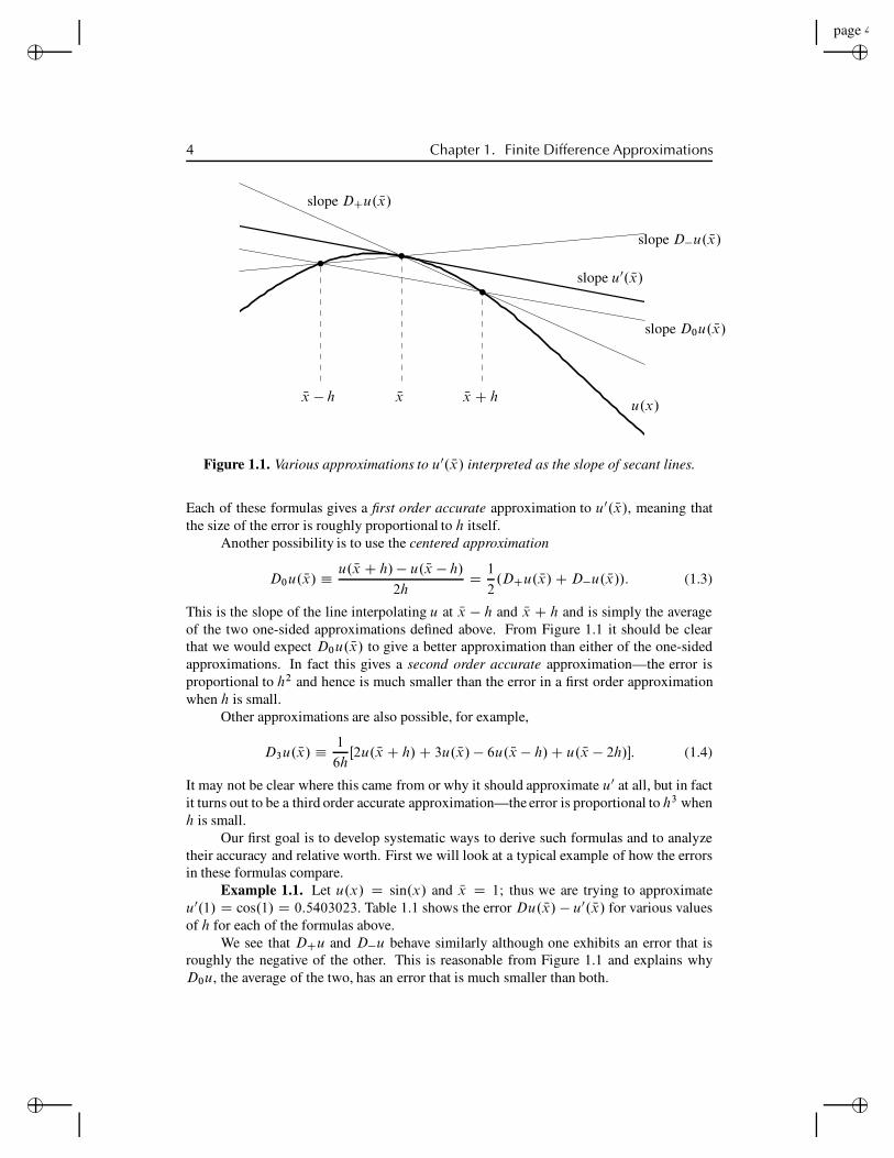
Figure 1.1. Various approximations to u0. Nx/ interpreted as the slope of secant lines.
Each of these formulas gives a first order accurate approximation to u0. Nx/, meaning thatthe size of the error is roughly proportional to h itself.
Another possibility is to use the centered approximation
D0u. Nx/ " u. Nx C h/ ! u. Nx ! h/
2hD 1
2.DCu. Nx/C D!u. Nx//: (1.3)
This is the slope of the line interpolating u at Nx ! h and Nx C h and is simply the averageof the two one-sided approximations defined above. From Figure 1.1 it should be clearthat we would expect D0u. Nx/ to give a better approximation than either of the one-sidedapproximations. In fact this gives a second order accurate approximation—the error isproportional to h2 and hence is much smaller than the error in a first order approximationwhen h is small.
Other approximations are also possible, for example,
D3u. Nx/ " 1
6hŒ2u. Nx C h/C 3u. Nx/ ! 6u. Nx ! h/C u. Nx ! 2h/!: (1.4)
It may not be clear where this came from or why it should approximate u0 at all, but in factit turns out to be a third order accurate approximation—the error is proportional to h3 whenh is small.
Our first goal is to develop systematic ways to derive such formulas and to analyzetheir accuracy and relative worth. First we will look at a typical example of how the errorsin these formulas compare.
Example 1.1. Let u.x/ D sin.x/ and Nx D 1; thus we are trying to approximateu0.1/ D cos.1/ D 0:5403023. Table 1.1 shows the error Du. Nx/ ! u0. Nx/ for various valuesof h for each of the formulas above.
We see that DCu and D!u behave similarly although one exhibits an error that isroughly the negative of the other. This is reasonable from Figure 1.1 and explains whyD0u, the average of the two, has an error that is much smaller than both.

“rjlfdm”2007/6/1page 5✐
✐✐
✐
✐✐
✐✐
1.1. Truncation errors 5
Table 1.1. Errors in various finite difference approximations to u0. Nx/.
h DCu. Nx/ D!u. Nx/ D0u. Nx/ D3u. Nx/1.0e!01 !4.2939e!02 4.1138e!02 !9.0005e!04 6.8207e!055.0e!02 !2.1257e!02 2.0807e!02 !2.2510e!04 8.6491e!061.0e!02 !4.2163e!03 4.1983e!03 !9.0050e!06 6.9941e!085.0e!03 !2.1059e!03 2.1014e!03 !2.2513e!06 8.7540e!091.0e!03 !4.2083e!04 4.2065e!04 !9.0050e!08 6.9979e!11
We see that
DCu. Nx/ ! u0. Nx/ " !0:42h;
D0u. Nx/ ! u0. Nx/ " !0:09h2;
D3u. Nx/ ! u0. Nx/ " 0:007h3;
confirming that these methods are first order, second order, and third order accurate,respectively.
Figure 1.2 shows these errors plotted against h on a log-log scale. This is a good wayto plot errors when we expect them to behave like some power of h, since if the error E.h/behaves like
E.h/ " C hp;
thenlog jE.h/j " log jC j C p log h:
So on a log-log scale the error behaves linearly with a slope that is equal to p, the order ofaccuracy.
1.1 Truncation errorsThe standard approach to analyzing the error in a finite difference approximation is toexpand each of the function values of u in a Taylor series about the point Nx, e.g.,
u. Nx C h/ D u. Nx/C hu0. Nx/C 1
2h2u00. Nx/C 1
6h3u000. Nx/C O.h4/; (1.5a)
u. Nx ! h/ D u. Nx/ ! hu0. Nx/C 1
2h2u00. Nx/ ! 1
6h3u000. Nx/C O.h4/: (1.5b)
These expansions are valid provided that u is sufficiently smooth. Readers unfamiliar withthe “big-oh” notation O.h4/ are advised to read Section A.2 of Appendix A at this pointsince this notation will be heavily used and a proper understanding of its use is critical.
Using (1.5a) allows us to compute that
DCu. Nx/ D u. Nx C h/ ! u. Nx/h
D u0. Nx/C 1
2hu00. Nx/C 1
6h2u000. Nx/C O.h3/:

“rjlfdm”2007/6/1page 6✐
✐✐
✐
✐✐
✐✐
6 Chapter 1. Finite Difference Approximations
10−3
10−2
10−1
10−10
10−8
10−6
10−4
10−2
DC
D0
D3
Figure 1.2. The errors in Du. Nx/ from Table 1.1 plotted against h on a log-log scale.
Recall that Nx is a fixed point so that u00. Nx/; u000. Nx/, etc., are fixed constants independent ofh. They depend on u of course, but the function is also fixed as we vary h.
For h sufficiently small, the error will be dominated by the first term 12hu00. Nx/ and all
the other terms will be negligible compared to this term, so we expect the error to behaveroughly like a constant times h, where the constant has the value 1
2u00. Nx/.
Note that in Example 1.1, where u.x/ D sin x, we have 12u00.1/ D !0:4207355,
which agrees with the behavior seen in Table 1.1.Similarly, from (1.5b) we can compute that the error in D!u. Nx/ is
D!u. Nx/ ! u0. Nx/ D !1
2hu00. Nx/C 1
6h2u000. Nx/C O.h3/;
which also agrees with our expectations.Combining (1.5a) and (1.5b) shows that
u. Nx C h/ ! u. Nx ! h/ D 2hu0. Nx/C 1
3h3u000. Nx/C O.h5/
so that
D0u. Nx/ ! u0. Nx/ D 1
6h2u000. Nx/C O.h4/: (1.6)
This confirms the second order accuracy of this approximation and again agrees with whatis seen in Table 1.1, since in the context of Example 1.1 we have
1
6u000. Nx/ D !1
6cos.1/ D !0:09005038:
Note that all the odd order terms drop out of the Taylor series expansion (1.6) for D0u. Nx/.This is typical with centered approximations and typically leads to a higher order approxi-mation.
“rjlfdm”2007/6/1page 7✐
✐✐
✐
✐✐
✐✐
1.2. Deriving finite difference approximations 7
To analyze D3u we need to also expand u. Nx ! 2h/ as
u. Nx ! 2h/ D u. Nx/ ! 2hu0. Nx/C 1
2.2h/2u00. Nx/ ! 1
6.2h/3u000. Nx/C O.h4/: (1.7)
Combining this with (1.5a) and (1.5b) shows that
D3u. Nx/ D u0. Nx/C 1
12h3u.4/. Nx/C O.h4/; (1.8)
where u.4/ is the fourth derivative of u.
1.2 Deriving finite difference approximationsSuppose we want to derive a finite difference approximation to u0. Nx/ based on some givenset of points. We can use Taylor series to derive an appropriate formula, using the methodof undetermined coefficients.
Example 1.2. Suppose we want a one-sided approximation to u0. Nx/ based on u. Nx/;u. Nx ! h/, and u. Nx ! 2h/ of the form
D2u. Nx/ D au. Nx/C bu. Nx ! h/C cu. Nx ! 2h/: (1.9)
We can determine the coefficients a; b, and c to give the best possible accuracy by expand-ing in Taylor series and collecting terms. Using (1.5b) and (1.7) in (1.9) gives
D2u. Nx/ D .a C b C c/u. Nx/ ! .b C 2c/hu0. Nx/C 1
2.b C 4c/h2u00. Nx/
! 1
6.b C 8c/h3u000. Nx/C " " " :
If this is going to agree with u0. Nx/ to high order, then we need
a C b C c D 0;
b C 2c D !1=h; (1.10)
b C 4c D 0:
We might like to require that higher order coefficients be zero as well, but since there areonly three unknowns a; b; and c, we cannot in general hope to satisfy more than three suchconditions. Solving the linear system (1.10) gives
a D 3=2h; b D !2=h; c D 1=2h
so that the formula is
D2u. Nx/ D 1
2hŒ3u. Nx/ ! 4u. Nx ! h/C u. Nx ! 2h/!: (1.11)
This approximation is used, for example, in the system of equations (2.57) for a 2-pointboundary value problem with a Neumann boundary condition at the left boundary.
“rjlfdm”2007/6/1page 8✐
✐✐
✐
✐✐
✐✐
8 Chapter 1. Finite Difference Approximations
The error in this approximation is
D2u. Nx/ ! u0. Nx/ D !1
6.b C 8c/h3u000. Nx/C " " "
D 1
12h2u000. Nx/C O.h3/:
(1.12)
There are other ways to derive the same finite difference approximations. One wayis to approximate the function u.x/ by some polynomial p.x/ and then use p0. Nx/ as an ap-proximation to u0. Nx/. If we determine the polynomial by interpolating u at an appropriateset of points, then we obtain the same finite difference methods as above.
Example 1.3. To derive the method of Example 1.2 in this way, let p.x/ be thequadratic polynomial that interpolates u at Nx, Nx ! h and Nx ! 2h, and then compute p0. Nx/.The result is exactly (1.11).
1.3 Second order derivativesApproximations to the second derivative u00.x/ can be obtained in an analogous manner.The standard second order centered approximation is given by
D2u. Nx/ D 1
h2Œu. Nx ! h/ ! 2u. Nx/C u. Nx C h/!
D u00. Nx/C 1
12h2u0000. Nx/C O.h4/:
(1.13)
Again, since this is a symmetric centered approximation, all the odd order terms drop out.This approximation can also be obtained by the method of undetermined coefficients, oralternatively by computing the second derivative of the quadratic polynomial interpolatingu.x/ at Nx ! h; Nx, and Nx C h, as is done in Example 1.4 below for the more general case ofunequally spaced points.
Another way to derive approximations to higher order derivatives is by repeatedlyapplying first order differences. Just as the second derivative is the derivative of u0, we canview D2u. Nx/ as being a difference of first differences. In fact,
D2u. Nx/ D DCD!u. Nx/since
DC.D!u. Nx// D 1
hŒD!u. Nx C h/ ! D!u. Nx/!
D 1
h
!"u. Nx C h/ ! u. Nx/
h
#!"
u. Nx/ ! u. Nx ! h/
h
#$
D D2u. Nx/:Alternatively, D2. Nx/ D D!DCu. Nx/, or we can also view it as a centered difference ofcentered differences, if we use a step size h=2 in each centered approximation to the firstderivative. If we define
OD0u.x/ D 1
h
"u
"x C h
2
#! u
"x ! h
2
##;
“rjlfdm”2007/6/1page 9✐
✐✐
✐
✐✐
✐✐
1.4. Higher order derivatives 9
then we find that
OD0. OD0u. Nx// D 1
h
!!u. Nx C h/ ! u. Nx/
h
"!!
u. Nx/ ! u. Nx ! h/
h
""D D2u. Nx/:
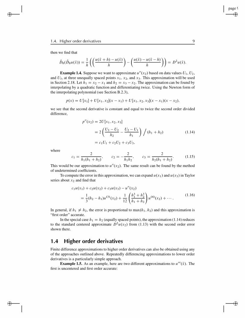
Example 1.4. Suppose we want to approximate u00.x2/ based on data values U1, U2,and U3, at three unequally spaced points x1; x2, and x3. This approximation will be usedin Section 2.18. Let h1 D x2 ! x1 and h2 D x3 ! x2. The approximation can be found byinterpolating by a quadratic function and differentiating twice. Using the Newton form ofthe interpolating polynomial (see Section B.2.3),
p.x/ D U Œx1! C U Œx1;x2!.x ! x1/C U Œx1;x2;x3!.x ! x1/.x ! x2/;
we see that the second derivative is constant and equal to twice the second order divideddifference,
p00.x2/ D 2U Œx1;x2;x3!
D 2
!U3 ! U2
h2! U2 ! U1
h1
" ..h1 C h2/
D c1U1 C c2U2 C c3U3;
(1.14)
where
c1 D 2
h1.h1 C h2/; c2 D ! 2
h1h2; c3 D 2
h2.h1 C h2/: (1.15)
This would be our approximation to u00.x2/. The same result can be found by the methodof undetermined coefficients.
To compute the error in this approximation, we can expand u.x1/ and u.x3/ in Taylorseries about x2 and find that
c1u.x1/C c2u.x2/C c3u.x3/ ! u00.x2/
D 1
3.h2 ! h1/u
.3/.x2/C 1
12
h3
1 C h32
h1 C h2
!u.4/.x2/C " " " :
(1.16)
In general, if h1 ¤ h2, the error is proportional to max.h1; h2/ and this approximation is“first order” accurate.
In the special case h1 D h2 (equally spaced points), the approximation (1.14) reducesto the standard centered approximate D2u.x2/ from (1.13) with the second order errorshown there.
1.4 Higher order derivativesFinite difference approximations to higher order derivatives can also be obtained using anyof the approaches outlined above. Repeatedly differencing approximations to lower orderderivatives is a particularly simple approach.
Example 1.5. As an example, here are two different approximations to u000. Nx/. Thefirst is uncentered and first order accurate:

“rjlfdm”2007/6/1page 10✐
✐✐
✐
✐✐
✐✐
10 Chapter 1. Finite Difference Approximations
DCD2u. Nx/ D 1
h3.u. Nx C 2h/ ! 3u. Nx C h/C 3u. Nx/ ! u. Nx ! h//
D u000. Nx/C 1
2hu0000. Nx/C O.h2/:
The next approximation is centered and second order accurate:
D0DCD!u. Nx/ D 1
2h3.u. Nx C 2h/ ! 2u. Nx C h/C 2u. Nx ! h/ ! u. Nx ! 2h//
D u000. Nx/C 1
4h2u00000. Nx/C O.h4/:
Another way to derive finite difference approximations to higher order derivativesis by interpolating with a sufficiently high order polynomial based on function values atthe desired stencil points and then computing the appropriate derivative of this polynomial.This is generally a cumbersome way to do it. A simpler approach that lends itself well toautomation is to use the method of undetermined coefficients, as illustrated in Section 1.2for an approximation to the first order derivative and explained more generally in the nextsection.
1.5 A general approach to deriving the coefficientsThe method illustrated in Section 1.2 can be extended to compute the finite difference co-efficients for computing an approximation to u.k/. Nx/, the kth derivative of u.x/ evaluatedat Nx, based on an arbitrary stencil of n " k C 1 points x1; : : : ; xn. Usually Nx is one of thestencil points, but not necessarily.
We assume u.x/ is sufficiently smooth, namely, at least n C 1 times continuouslydifferentiable in the interval containing Nx and all the stencil points, so that the Taylor seriesexpansions below are valid. Taylor series expansions of u at each point xi in the stencilabout u. Nx/ yield
u.xi/ D u. Nx/C .xi ! Nx/u0. Nx/C # # # C 1
k!.xi ! Nx/k u.k/. Nx/C # # # (1.17)
for i D 1; : : : ; n. We want to find a linear combination of these values that agrees withu.k/. Nx/ as well as possible. So we want
c1u.x1/C c2u.x2/C # # # C cnu.xn/ D u.k/. Nx/C O.hp /; (1.18)
where p is as large as possible. (Here h is some measure of the width of the stencil. Ifwe are deriving approximations on stencils with equally spaced points, then h is the meshwidth, but more generally it is some “average mesh width,” so that max1"i"n jxi! Nxj $ C hfor some small constant C .)
Following the approach of Section 1.2, we choose the coefficients cj so that
1
.i ! 1/!
nX
jD1
cj .xj ! Nx/.i!1/ D!
1 if i ! 1 D k;0 otherwise (1.19)
for i D 1; : : : ; n. Provided the points xj are distinct, this n % n Vandermonde system isnonsingular and has a unique solution. If n $ k (too few points in the stencil), then the
“rjlfdm”2007/6/1page 11✐
✐✐
✐
✐✐
✐✐
1.5. A general approach to deriving the coefficients 11
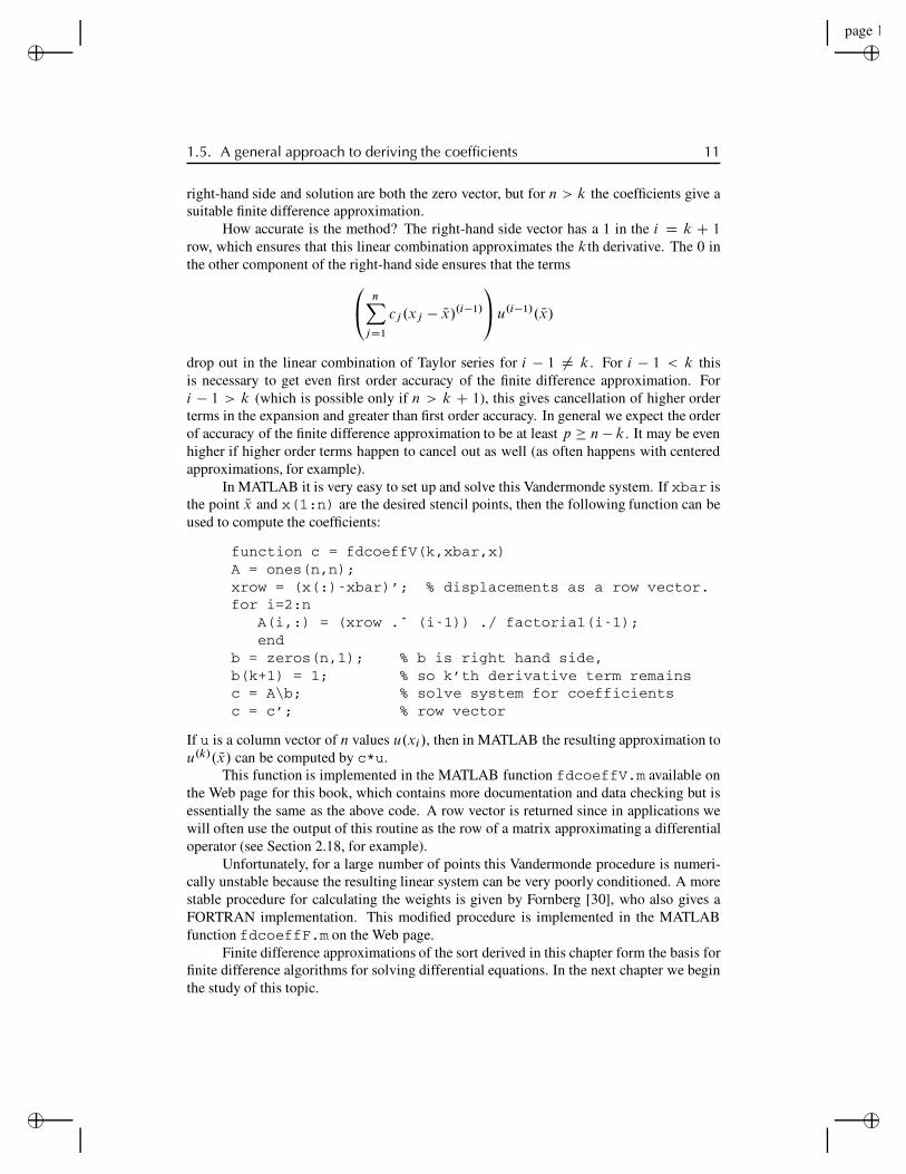
right-hand side and solution are both the zero vector, but for n > k the coefficients give asuitable finite difference approximation.
How accurate is the method? The right-hand side vector has a 1 in the i D k C 1row, which ensures that this linear combination approximates the kth derivative. The 0 inthe other component of the right-hand side ensures that the terms
0
@nX
jD1
cj .xj ! Nx/.i!1/
1
Au.i!1/. Nx/
drop out in the linear combination of Taylor series for i ! 1 ¤ k . For i ! 1 < k thisis necessary to get even first order accuracy of the finite difference approximation. Fori ! 1 > k (which is possible only if n > k C 1), this gives cancellation of higher orderterms in the expansion and greater than first order accuracy. In general we expect the orderof accuracy of the finite difference approximation to be at least p " n ! k . It may be evenhigher if higher order terms happen to cancel out as well (as often happens with centeredapproximations, for example).
In MATLAB it is very easy to set up and solve this Vandermonde system. If xbar isthe point Nx and x(1:n) are the desired stencil points, then the following function can beused to compute the coefficients:
function c = fdcoeffV(k,xbar,x)A = ones(n,n);xrow = (x(:)-xbar)’; % displacements as a row vector.for i=2:n
A(i,:) = (xrow .ˆ (i-1)) ./ factorial(i-1);end
b = zeros(n,1); % b is right hand side,b(k+1) = 1; % so k’th derivative term remainsc = A\b; % solve system for coefficientsc = c’; % row vector
If u is a column vector of n values u.xi/, then in MATLAB the resulting approximation tou.k/. Nx/ can be computed by c*u.
This function is implemented in the MATLAB function fdcoeffV.m available onthe Web page for this book, which contains more documentation and data checking but isessentially the same as the above code. A row vector is returned since in applications wewill often use the output of this routine as the row of a matrix approximating a differentialoperator (see Section 2.18, for example).
Unfortunately, for a large number of points this Vandermonde procedure is numeri-cally unstable because the resulting linear system can be very poorly conditioned. A morestable procedure for calculating the weights is given by Fornberg [30], who also gives aFORTRAN implementation. This modified procedure is implemented in the MATLABfunction fdcoeffF.m on the Web page.
Finite difference approximations of the sort derived in this chapter form the basis forfinite difference algorithms for solving differential equations. In the next chapter we beginthe study of this topic.

“rjlfdm”2007/6/1page 12✐
✐✐
✐
✐✐
✐✐

“rjlfdm”2007/6/1page 13✐
✐✐
✐
✐✐
✐✐
Chapter 2
Steady States and BoundaryValue Problems
We will first consider ordinary differential equations (ODEs) that are posed on some in-terval a < x < b, together with some boundary conditions at each end of the interval.In the next chapter we will extend this to more than one space dimension and will studyelliptic partial differential equations (ODEs) that are posed in some region of the plane orthree-dimensional space and are solved subject to some boundary conditions specifying thesolution and/or its derivatives around the boundary of the region. The problems consideredin these two chapters are generally steady-state problems in which the solution varies onlywith the spatial coordinates but not with time. (But see Section 2.16 for a case where Œa; b!is a time interval rather than an interval in space.)
Steady-state problems are often associated with some time-dependent problem thatdescribes the dynamic behavior, and the 2-point boundary value problem (BVP) or ellipticequation results from considering the special case where the solution is steady in time, andhence the time-derivative terms are equal to zero, simplifying the equations.
2.1 The heat equationAs a specific example, consider the flow of heat in a rod made out of some heat-conductingmaterial, subject to some external heat source along its length and some boundary condi-tions at each end. If we assume that the material properties, the initial temperature distri-bution, and the source vary only with x, the distance along the length, and not across anycross section, then we expect the temperature distribution at any time to vary only withx and we can model this with a differential equation in one space dimension. Since thesolution might vary with time, we let u.x; t/ denote the temperature at point x at time t ,where a < x < b along some finite length of the rod. The solution is then governed by theheat equation
ut .x; t/ D .".x/ux .x; t//x C .x; t/; (2.1)
where ".x/ is the coefficient of heat conduction, which may vary with x, and .x; t/ isthe heat source (or sink, if < 0). See Appendix E for more discussion and a derivation.Equation (2.1) is often called the diffusion equation since it models diffusion processesmore generally, and the diffusion of heat is just one example. It is assumed that the basic
13

“rjlfdm”2007/6/1page 14✐
✐✐
✐
✐✐
✐✐
14 Chapter 2. Steady States and Boundary Value Problems
theory of this equation is familiar to the reader. See standard PDE books such as [55]for a derivation and more introduction. In general it is extremely valuable to understandwhere the equation one is attempting to solve comes from, since a good understanding ofthe physics (or biology, etc.) is generally essential in understanding the development andbehavior of numerical methods for solving the equation.
2.2 Boundary conditionsIf the material is homogeneous, then !.x/ ! ! is independent of x and the heat equation(2.1) reduces to
ut.x; t/ D !uxx.x; t/C .x; t/: (2.2)
Along with the equation, we need initial conditions,
u.x; 0/ D u0.x/;
and boundary conditions, for example, the temperature might be specified at each end,
u.a; t/ D ˛.t/; u.b; t/ D ˇ.t/: (2.3)
Such boundary conditions, where the value of the solution itself is specified, are calledDirichlet boundary conditions. Alternatively one end, or both ends, might be insulated, inwhich case there is zero heat flux at that end, and so ux D 0 at that point. This boundarycondition, which is a condition on the derivative of u rather than on u itself, is called aNeumann boundary condition. To begin, we will consider the Dirichlet problem for (2.2)with boundary conditions (2.3).
2.3 The steady-state problemIn general we expect the temperature distribution to change with time. However, if .x; t/,˛.t/, and ˇ.t/ are all time independent, then we might expect the solution to eventuallyreach a steady-state solution u.x/, which then remains essentially unchanged at later times.Typically there will be an initial transient time, as the initial data u0.x/ approach u.x/(unless u0.x/ ! u.x/), but if we are interested only in computing the steady-state solutionitself, then we can set ut D 0 in (2.2) and obtain an ODE in x to solve for u.x/:
u00.x/ D f .x/; (2.4)
where we introduce f .x/ D " .x/=! to avoid minus signs below. This is a second orderODE, and from basic theory we expect to need two boundary conditions to specify a uniquesolution. In our case we have the boundary conditions
u.a/ D ˛; u.b/ D ˇ: (2.5)
Remark: Having two boundary conditions does not necessarily guarantee that thereexists a unique solution for a general second order equation—see Section 2.13.
The problem (2.4), (2.5) is called a 2-point (BVP), since one condition is specified ateach of the two endpoints of the interval where the solution is desired. If instead two data
“rjlfdm”2007/6/1page 15✐
✐✐
✐
✐✐
✐✐
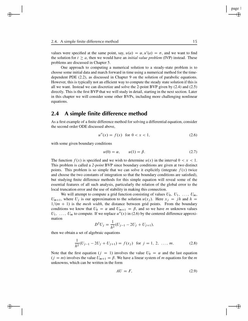
2.4. A simple finite difference method 15
values were specified at the same point, say, u.a/ D ˛;u0.a/ D ! , and we want to findthe solution for t ! a, then we would have an initial value problem (IVP) instead. Theseproblems are discussed in Chapter 5.
One approach to computing a numerical solution to a steady-state problem is tochoose some initial data and march forward in time using a numerical method for the time-dependent PDE (2.2), as discussed in Chapter 9 on the solution of parabolic equations.However, this is typically not an efficient way to compute the steady state solution if this isall we want. Instead we can discretize and solve the 2-point BVP given by (2.4) and (2.5)directly. This is the first BVP that we will study in detail, starting in the next section. Laterin this chapter we will consider some other BVPs, including more challenging nonlinearequations.
2.4 A simple finite difference methodAs a first example of a finite difference method for solving a differential equation, considerthe second order ODE discussed above,
u00.x/ D f .x/ for 0 < x < 1; (2.6)
with some given boundary conditions
u.0/ D ˛; u.1/ D ˇ: (2.7)
The function f .x/ is specified and we wish to determine u.x/ in the interval 0 < x < 1.This problem is called a 2-point BVP since boundary conditions are given at two distinctpoints. This problem is so simple that we can solve it explicitly (integrate f .x/ twiceand choose the two constants of integration so that the boundary conditions are satisfied),but studying finite difference methods for this simple equation will reveal some of theessential features of all such analysis, particularly the relation of the global error to thelocal truncation error and the use of stability in making this connection.
We will attempt to compute a grid function consisting of values U0; U1; : : : ; Um,UmC1, where Uj is our approximation to the solution u.xj /. Here xj D j h and h D1=.m C 1/ is the mesh width, the distance between grid points. From the boundaryconditions we know that U0 D ˛ and UmC1 D ˇ, and so we have m unknown valuesU1; : : : ; Um to compute. If we replace u00.x/ in (2.6) by the centered difference approxi-mation
D2Uj D 1
h2.Uj!1 " 2Uj C UjC1/;
then we obtain a set of algebraic equations
1
h2.Uj!1 " 2Uj C UjC1/ D f .xj / for j D 1; 2; : : : ; m: (2.8)
Note that the first equation .j D 1/ involves the value U0 D ˛ and the last equation.j D m/ involves the value UmC1 D ˇ. We have a linear system of m equations for the munknowns, which can be written in the form
AU D F; (2.9)
“rjlfdm”2007/6/1page 16✐
✐✐
✐
✐✐
✐✐
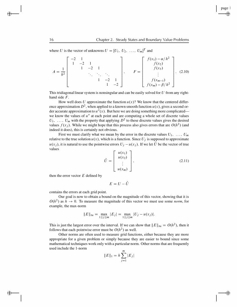
16 Chapter 2. Steady States and Boundary Value Problems
where U is the vector of unknowns U D ŒU1; U2; : : : ; Um!T and
A D 1
h2
2
66666664
!2 11 !2 1
1 !2 1: : :
: : :: : :
1 !2 11 !2
3
77777775
; F D
2
66666664
f .x1/ ! ˛=h2
f .x2/f .x3/:::
f .xm!1/
f .xm/ ! ˇ=h2
3
77777775
: (2.10)
This tridiagonal linear system is nonsingular and can be easily solved for U from any right-hand side F .
How well does U approximate the function u.x/? We know that the centered differ-ence approximation D2, when applied to a known smooth function u.x/, gives a second or-der accurate approximation to u00.x/. But here we are doing something more complicated—we know the values of u00 at each point and are computing a whole set of discrete valuesU1; : : : ; Um with the property that applying D2 to these discrete values gives the desiredvalues f .xj /. While we might hope that this process also gives errors that are O.h2/ (andindeed it does), this is certainly not obvious.
First we must clarify what we mean by the error in the discrete values U1; : : : ; Um
relative to the true solution u.x/, which is a function. Since Uj is supposed to approximateu.xj /, it is natural to use the pointwise errors Uj !u.xj /. If we let OU be the vector of truevalues
OU D
2
6664
u.x1/u.x2/:::
u.xm/
3
7775; (2.11)
then the error vector E defined by
E D U ! OU
contains the errors at each grid point.Our goal is now to obtain a bound on the magnitude of this vector, showing that it is
O.h2/ as h ! 0. To measure the magnitude of this vector we must use some norm, forexample, the max-norm
kEk1 D max1"j"m
jEj j D max1"j"m
jUj ! u.xj /j:
This is just the largest error over the interval. If we can show that kEk1 D O.h2/, then itfollows that each pointwise error must be O.h2/ as well.
Other norms are often used to measure grid functions, either because they are moreappropriate for a given problem or simply because they are easier to bound since somemathematical techniques work only with a particular norm. Other norms that are frequentlyused include the 1-norm
kEk1 D h
mX
jD1
jEj j

“rjlfdm”2007/6/1page 17✐
✐✐
✐
✐✐
✐✐
2.5. Local truncation error 17
and the 2-norm
kEk2 D
0
@h
mX
jD1
jEj j21
A1=2
:
Note the factor of h that appears in these definitions. See Appendix A for a more thoroughdiscussion of grid function norms and how they relate to standard vector norms.
Now let’s return to the problem of estimating the error in our finite difference solutionto BVP obtained by solving the system (2.9). The technique we will use is absolutely basicto the analysis of finite difference methods in general. It involves two key steps. We firstcompute the local truncation error (LTE) of the method and then use some form of stabilityto show that the global error can be bounded in terms of the LTE.
The global error simply refers to the error U ! OU that we are attempting to bound.The LTE refers to the error in our finite difference approximation of derivatives and henceis something that can be easily estimated using Taylor series expansions, as we have seen inChapter 1. Stability is the magic ingredient that allows us to go from these easily computedbounds on the local error to the estimates we really want for the global error. Let’s look ateach of these in turn.
2.5 Local truncation errorThe LTE is defined by replacing Uj with the true solution u.xj / in the finite differenceformula (2.8). In general the true solution u.xj / won’t satisfy this equation exactly and thediscrepancy is the LTE, which we denote by !j :
!j D 1
h2.u.xj!1/ ! 2u.xj /C u.xjC1// ! f .xj / (2.12)
for j D 1; 2; : : : ; m. Of course in practice we don’t know what the true solution u.x/ is,but if we assume it is smooth, then by the Taylor series expansions (1.5a) we know that
!j D!u00.xj /C 1
12h2u0000.xj /C O.h4/
"! f .xj /: (2.13)
Using our original differential equation (2.6) this becomes
!j D 1
12h2u0000.xj /C O.h4/:
Although u0000 is in general unknown, it is some fixed function independent of h, and so!j D O.h2/ as h ! 0.
If we define ! to be the vector with components !j , then
! D A OU ! F;
where OU is the vector of true solution values (2.11), and so
A OU D F C !: (2.14)
“rjlfdm”2007/6/1page 18✐
✐✐
✐
✐✐
✐✐
18 Chapter 2. Steady States and Boundary Value Problems
2.6 Global errorTo obtain a relation between the local error ! and the global error E D U ! OU , we subtract(2.14) from (2.9) that defines U , obtaining
AE D !!: (2.15)
This is simply the matrix form of the system of equations
1
h2.Ej!1 ! 2Ej C EjC1/ D !!.xj / for j D 1; 2; : : : ; m
with the boundary conditionsE0 D EmC1 D 0
since we are using the exact boundary data U0 D ˛ and UmC1 D ˇ. We see that theglobal error satisfies a set of finite difference equations that has exactly the same form asour original difference equations for U except that the right-hand side is given by !! ratherthan F .
From this it should be clear why we expect the global error to be roughly the samemagnitude as the local error ! . We can interpret the system (2.15) as a discretization of theODE
e00.x/ D !!.x/ for 0 < x < 1 (2.16)
with boundary conditionse.0/ D 0; e.1/ D 0:
Since !.x/ " 112
h2u0000.x/, integrating twice shows that the global error should be roughly
e.x/ " ! 1
12h2u00.x/C 1
12h2!u00.0/C x.u00.1/ ! u00.0//
"
and hence the error should be O.h2/.
2.7 StabilityThe above argument is not completely convincing because we are relying on the assump-tion that solving the difference equations gives a decent approximation to the solution ofthe underlying differential equations (actually the converse now, that the solution to the dif-ferential equation (2.16) gives a good indication of the solution to the difference equations(2.15)). Since it is exactly this assumption we are trying to prove, the reasoning is rathercircular.
Instead, let’s look directly at the discrete system (2.15), which we will rewrite in theform
AhEh D !!h; (2.17)
where the superscript h indicates that we are on a grid with mesh spacing h. This serves asa reminder that these quantities change as we refine the grid. In particular, the matrix Ah isan m # m matrix with h D 1=.m C 1/ so that its dimension is growing as h ! 0.
“rjlfdm”2007/6/1page 19✐
✐✐
✐
✐✐
✐✐
2.9. Convergence 19
Let .Ah/!1 be the inverse of this matrix. Then solving the system (2.17) gives
Eh D !.Ah/!1!h
and taking norms gives
kEhk D k.Ah/!1!hk" k.Ah/!1k k!hk:
We know that k!hk D O.h2/ and we are hoping the same will be true of kEhk. It isclear what we need for this to be true: we need k.Ah/!1k to be bounded by some constantindependent of h as h ! 0:
k.Ah/!1k " C for all h sufficiently small:
Then we will havekEhk " C k!hk (2.18)
and so kEhk goes to zero at least as fast as k!hk. This motivates the following definitionof stability for linear BVPs.
Definition 2.1. Suppose a finite difference method for a linear BVP gives a sequence ofmatrix equations of the form AhU h D F h, where h is the mesh width. We say that themethod is stable if .Ah/!1 exists for all h sufficiently small (for h < h0, say) and if there isa constant C , independent of h, such that
k.Ah/!1k " C for all h < h0: (2.19)
2.8 ConsistencyWe say that a method is consistent with the differential equation and boundary conditionsif
k!hk ! 0 as h ! 0: (2.20)
This simply says that we have a sensible discretization of the problem. Typically k!hk DO.hp / for some integer p > 0, and then the method is certainly consistent.
2.9 ConvergenceA method is said to be convergent if kEhk ! 0 as h ! 0. Combining the ideas introducedabove we arrive at the conclusion that
consistency C stability H) convergence: (2.21)
This is easily proved by using (2.19) and (2.20) to obtain the bound
kEhk " k.Ah/!1k k!hk " C k!hk ! 0 as h ! 0:
“rjlfdm”2007/6/1page 20✐
✐✐
✐
✐✐
✐✐
20 Chapter 2. Steady States and Boundary Value Problems
Although this has been demonstrated only for the linear BVP, in fact most analyses of finitedifference methods for differential equations follow this same two-tier approach, and thestatement (2.21) is sometimes called the fundamental theorem of finite difference methods.In fact, as our above analysis indicates, this can generally be strengthened to say that
O.hp/ local truncation error C stability H) O.hp / global error. (2.22)
Consistency (and the order of accuracy) is usually the easy part to check. Verifying sta-bility is the hard part. Even for the linear BVP just discussed it is not at all clear how tocheck the condition (2.19) since these matrices become larger as h ! 0. For other prob-lems it may not even be clear how to define stability in an appropriate way. As we will see,there are many definitions of “stability” for different types of problems. The challenge inanalyzing finite difference methods for new classes of problems often is to find an appro-priate definition of “stability” that allows one to prove convergence using (2.21) while atthe same time being sufficiently manageable that we can verify it holds for specific finitedifference methods. For nonlinear PDEs this frequently must be tuned to each particularclass of problems and relies on existing mathematical theory and techniques of analysis forthis class of problems.
Whether or not one has a formal proof of convergence for a given method, it is alwaysgood practice to check that the computer program is giving convergent behavior, at the rateexpected. Appendix A contains a discussion of how the error in computed results can beestimated.
2.10 Stability in the 2-normReturning to the BVP at the start of the chapter, let’s see how we can verify stability andhence second order accuracy. The technique used depends on what norm we wish to con-sider. Here we will consider the 2-norm and see that we can show stability by explicitlycomputing the eigenvectors and eigenvalues of the matrix A. In Section 2.11 we showstability in the max-norm by different techniques.
Since the matrix A from (2.10) is symmetric, the 2-norm of A is equal to its spectralradius (see Section A.3.2 and Section C.9):
kAk2 D !.A/ D max1!p!m
j"pj:
(Note that "p refers to the pth eigenvalue of the matrix. Superscripts are used to index theeigenvalues and eigenvectors, while subscripts on the eigenvector below refer to compo-nents of the vector.)
The matrix A"1 is also symmetric, and the eigenvalues of A"1 are simply the inversesof the eigenvalues of A, so
kA"1k2 D !.A"1/ D max1!p!m
j."p/"1j D
!min
1!p!mj"pj
""1
:
So all we need to do is compute the eigenvalues of A and show that they are boundedaway from zero as h ! 0. Of course we have an infinite set of matrices Ah to consider,

“rjlfdm”2007/6/1page 21✐
✐✐
✐
✐✐
✐✐
2.10. Stability in the 2-norm 21
as h varies, but since the structure of these matrices is so simple, we can obtain a generalexpression for the eigenvalues of each Ah. For more complicated problems we mightnot be able to do this, but it is worth going through in detail for this problem becauseone often considers model problems for which such an analysis is possible. We will alsoneed to know these eigenvalues for other purposes when we discuss parabolic equationsin Chapter 9. (See also Section C.7 for more general expressions for the eigenvalues ofrelated matrices.)
We will now focus on one particular value of h D 1=.mC1/ and drop the superscripth to simplify the notation. Then the m eigenvalues of A are given by
!p D 2
h2.cos.p"h/ ! 1/ for p D 1; 2; : : : ; m: (2.23)
The eigenvector up corresponding to !p has components upj for j D 1; 2; : : : ; m
given byu
pj D sin.p"j h/: (2.24)
This can be verified by checking that Aup D !pup . The j th component of the vectorAup is
.Aup /j D 1
h2
!u
pj!1 ! 2u
pj C u
pjC1
"
D 1
h2.sin.p".j ! 1/h/ ! 2 sin.p"j h/C sin.p".j C 1/h//
D 1
h2.sin.p"j h/ cos.p"h/ ! 2 sin.p"j h/C sin.p"j h/ cos.p"h//
D !pupj :
Note that for j D 1 and j D m the j th component of Aup looks slightly different (theup
j!1 or upjC1 term is missing) but that the above form and trigonometric manipulations are
still valid provided that we define
up0 D u
pmC1 D 0;
as is consistent with (2.24). From (2.23) we see that the smallest eigenvalue of A (inmagnitude) is
!1 D 2
h2.cos."h/ ! 1/
D 2
h2
#!1
2"2h2 C 1
24"4h4 C O.h6/
$
D !"2 C O.h2/:
This is clearly bounded away from zero as h ! 0, and so we see that the method is stablein the 2-norm. Moreover we get an error bound from this:
kEhk2 " k.Ah/!1k2k#hk2 #1
"2k#hk2:
“rjlfdm”2007/6/1page 22✐
✐✐
✐
✐✐
✐✐
22 Chapter 2. Steady States and Boundary Value Problems
Since !hj ! 1
12 h2u0000.xj /, we expect k!hk2 ! 112 h2ku0000k2 D 1
12 h2kf 00k2. The 2-norm ofthe function f 00 here means the grid-function norm of this function evaluated at the discretepoints xj , although this is approximately equal to the function space norm of f 00 definedusing (A.14).
Note that the eigenvector (2.24) is closely related to the eigenfunction of the corre-sponding differential operator @2
@x2 . The functions
up.x/ D sin.p"x/; p D 1; 2; 3; : : : ;
satisfy the relation@2
@x2up.x/ D #pup.x/
with eigenvalue #p D "p2"2. These functions also satisfy up.0/ D up.1/ D 0, andhence they are eigenfunctions of @2
@x2 on Œ0; 1$ with homogeneous boundary conditions.The discrete approximation to this operator given by the matrix A has only m eigenvaluesinstead of an infinite number, and the corresponding eigenvectors (2.24) are simply the firstm eigenfunctions of @2
@x2 evaluated at the grid points. The eigenvalue %p is not exactly thesame as #p , but at least for small values of p it is very nearly the same, since Taylor seriesexpansion of the cosine in (2.23) gives
%p D 2
h2
!"1
2p2"2h2 C 1
24p4"4h4 C # # #
"
D "p2"2 C O.h2/ as h ! 0 for p fixed.
This relationship will be illustrated further when we study numerical methods for the heatequation (2.1).
2.11 Green’s functions and max-norm stabilityIn Section 2.10 we demonstrated that A from (2.10) is stable in the 2-norm, and hence thatkEk2 D O.h2/. Suppose, however, that we want a bound on the maximum error over theinterval, i.e., a bound on kEk1 D max jEj j. We can obtain one such bound directly fromthe bound we have for the 2-norm. From (A.19) we know that
kEk1 $ 1ph
kEk2 D O.h3=2/ as h ! 0:
However, this does not show the second order accuracy that we hope to have. To showthat kEk1 D O.h2/ we will explicitly calculate the inverse of A and then show thatkA!1k1 D O.1/, and hence
kEk1 $ kA!1k1k!k1 D O.h2/
since k!k1 D O.h2/. As in the computation of the eigenvalues in the last section, wecan do this only because our model problem (2.6) is so simple. In general it would beimpossible to obtain closed form expressions for the inverse of the matrices Ah as h varies.

“rjlfdm”2007/6/1page 23✐
✐✐
✐
✐✐
✐✐
2.11. Green’s functions and max-norm stability 23
But again it is worth working out the details for this simple case because it gives a greatdeal of insight into the nature of the inverse matrix and what it represents more generally.
Each column of the inverse matrix can be interpreted as the solution of a particularBVP. The columns are discrete approximations to the Green’s functions that are commonlyintroduced in the study of the differential equation. An understanding of this is valuablein developing an intuition for what happens if we introduce relatively large errors at a fewpoints within the interval. Such difficulties arise frequently in practice, typically at theboundary or at an internal interface where there are discontinuities in the data or solution.
We begin by reviewing the Green’s function solution to the BVP
u00.x/ D f .x/ for 0 < x < 1 (2.25)
with Dirichlet boundary conditions
u.0/ D ˛; u.1/ D ˇ: (2.26)
To keep the expressions simple below we assume we are on the unit interval, but everythingcan be shifted to an arbitrary interval Œa; b!.
For any fixed point Nx 2 Œ0; 1!, the Green’s function G.xI Nx/ is the function of x thatsolves the particular BVP of the above form with f .x/ D ı.x ! Nx/ and ˛ D ˇ D 0.Here ı.x ! Nx/ is the “delta function” centered at Nx. The delta function, ı.x/, is not anordinary function but rather the mathematical idealization of a sharply peaked function thatis nonzero only on an interval .!"; "/ near the origin and has the property that
Z 1
!1#!.x/ dx D
Z !
!!
#!.x/ dx D 1: (2.27)
For example, we might take
#!.x/ D
8<
:
." C x/=" if ! " " x " 0;
." ! x/=" if 0 " x " ";0 otherwise:
(2.28)
This piecewise linear function is the “hat function” with width " and height 1=". Theexact shape of #! is not important, but note that it must attain a height that is O.1="/ inorder for the integral to have the value 1. We can think of the delta function as being asort of limiting case of such functions as " ! 0. Delta functions naturally arise when wedifferentiate functions that are discontinuous. For example, consider the Heaviside function(or step function) H .x/ that is defined by
H .x/ D!
0 x < 0;1 x # 0:
(2.29)
What is the derivative of this function? For x ¤ 0 the function is constant and so H 0.x/ D0. At x D 0 the derivative is not defined in the classical sense. But if we smooth outthe function a little bit, making it continuous and differentiable by changing H .x/ only onthe interval .!"; "/, then the new function H!.x/ is differentiable everywhere and has a
“rjlfdm”2007/6/1page 24✐
✐✐
✐
✐✐
✐✐
24 Chapter 2. Steady States and Boundary Value Problems
derivative H 0!.x/ that looks something like !!.x/. The exact shape of H 0
!.x/ depends onhow we choose H!.x/, but note that regardless of its shape, its integral must be 1, since
Z 1
!1H 0
!.x/ dx DZ !
!!
H 0!.x/ dx
D H!."/ ! H!.!"/D 1 ! 0 D 1:
This explains the normalization (2.27). By letting " ! 0, we are led to define
H 0.x/ D ı.x/:
This expression makes no sense in terms of the classical definition of derivatives, but it canbe made rigorous mathematically through the use of “distribution theory”; see, for example,[31]. For our purposes it suffices to think of the delta function as being a very sharplypeaked function that is nonzero only on a very narrow interval but with total integral 1.
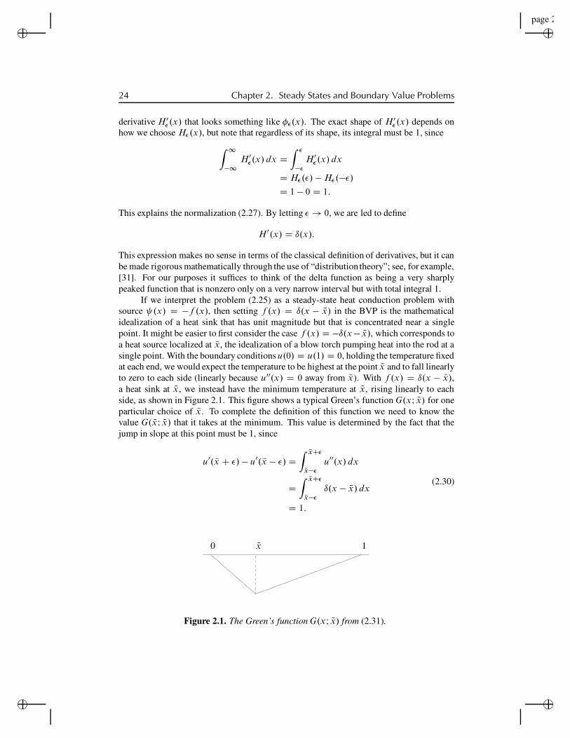
If we interpret the problem (2.25) as a steady-state heat conduction problem withsource .x/ D !f .x/, then setting f .x/ D ı.x ! Nx/ in the BVP is the mathematicalidealization of a heat sink that has unit magnitude but that is concentrated near a singlepoint. It might be easier to first consider the case f .x/ D !ı.x! Nx/, which corresponds toa heat source localized at Nx, the idealization of a blow torch pumping heat into the rod at asingle point. With the boundary conditions u.0/ D u.1/ D 0, holding the temperature fixedat each end, we would expect the temperature to be highest at the point Nx and to fall linearlyto zero to each side (linearly because u00.x/ D 0 away from Nx). With f .x/ D ı.x ! Nx/,a heat sink at Nx, we instead have the minimum temperature at Nx, rising linearly to eachside, as shown in Figure 2.1. This figure shows a typical Green’s function G.xI Nx/ for oneparticular choice of Nx. To complete the definition of this function we need to know thevalue G. NxI Nx/ that it takes at the minimum. This value is determined by the fact that thejump in slope at this point must be 1, since
u0. Nx C "/ ! u0. Nx ! "/ DZ NxC!
Nx!!
u00.x/ dx
DZ NxC!
Nx!!
ı.x ! Nx/ dx
D 1:
(2.30)
0 1Nx
Figure 2.1. The Green’s function G.xI Nx/ from (2.31).
“rjlfdm”2007/6/1page 25✐
✐✐
✐
✐✐
✐✐
2.11. Green’s functions and max-norm stability 25
A little algebra shows that the piecewise linear function G.xI Nx/ is given by
G.xI Nx/ D!. Nx ! 1/x for 0 " x " Nx;Nx.x ! 1/ for Nx " x " 1:
(2.31)
Note that by linearity, if we replaced f .x/ with cı.x ! Nx/ for any constant c, the solutionto the BVP would be cG.xI Nx/. Moreover, any linear combination of Green’s functions atdifferent points Nx is a solution to the BVP with the corresponding linear combination ofdelta functions on the right-hand side. So if we want to solve
u00.x/ D 3ı.x ! 0:3/ ! 5ı.x ! 0:7/; (2.32)
for example (with u.0/ D u.1/ D 0), the solution is simply
u.x/ D 3G.xI 0:3/! 5G.xI 0:7/: (2.33)
This is a piecewise linear function with jumps in slope of magnitude 3 at x D 0:3 and !5at x D 0:7. More generally, if the right-hand side is a sum of weighted delta functions atany number of points,
f .x/ DnX
kD1
ckı.x ! xk/; (2.34)
then the solution to the BVP is
u.x/ DnX
kD1
ckG.xI xk/: (2.35)
Now consider a general source f .x/ that is not a discrete sum of delta functions.We can view this as a continuous distribution of point sources, with f . Nx/ being a densityfunction for the weight assigned to the delta function at Nx, i.e.,
f .x/ DZ 1
0
f . Nx/ı.x ! Nx/ d Nx: (2.36)
(Note that if we smear out ı to !! , then the right-hand side becomes a weighted average ofvalues of f very close to x.) This suggests that the solution to u00.x/ D f .x/ (still withu.0/ D u.1/ D 0) is
u.x/ DZ 1
0
f . Nx/G.xI Nx/ d Nx; (2.37)
and indeed it is.Now let’s consider more general boundary conditions. Since each Green’s function
G.xI Nx/ satisfies the homogeneous boundary conditions u.0/ D u.1/ D 0, any linearcombination does as well. To incorporate the effect of nonzero boundary conditions, weintroduce two new functions G0.x/ and G1.x/ defined by the BVPs
G000.x/ D 0; G0.0/ D 1; G0.1/ D 0 (2.38)

“rjlfdm”2007/6/1page 26✐
✐✐
✐
✐✐
✐✐
26 Chapter 2. Steady States and Boundary Value Problems
and
G001 .x/ D 0; G1.0/ D 0; G1.1/ D 1: (2.39)
The solutions are
G0.x/ D 1 ! x;
G1.x/ D x:(2.40)
These functions give the temperature distribution for the heat conduction problem withthe temperature held at 1 at one boundary and 0 at the other with no internal heat source.Adding a scalar multiple of G0.x/ to the solution u.x/ of (2.37) will change the valueof u.0/ without affecting u00.x/ or u.1/, so adding ˛G0.x/ will allow us to satisfy theboundary condition at x D 0, and similarly adding ˇG1.x/ will give the desired boundaryvalue at x D 1. The full solution to (2.25) with boundary conditions (2.26) is thus
u.x/ D ˛G0.x/C ˇG1.x/CZ 1
0
f . Nx/G.xI Nx/ d Nx: (2.41)
Note that using the formula (2.31), we can rewrite this as
u.x/ D!˛ !
Z x
0
Nxf . Nx/ d Nx".1 ! x/C
ˇ C
Z 1
x
. Nx ! 1/f . Nx/ d Nx!
x: (2.42)
Of course this simple BVP can also be solved simply by integrating the function f twice,and the solution (2.42) can be put in this same form using integration by parts. But forour current purposes it is the form (2.41) that is of interest, since it shows clearly how theeffect of each boundary condition and the local source at each point feeds into the globalsolution. The values ˛; ˇ, and f .x/ are the data for this linear differential equation and(2.41) writes the solution as a linear operator applied to this data, analogous to writing thesolution to the linear system AU D F as U D A!1F .
We are finally ready to return to the study of the max-norm stability of the finitedifference method, which will be based on explicitly determining the inverse matrix for thematrix arising in this discretization. We will work with a slightly different formulation ofthe linear algebra problem in which we view U0 and UmC1 as additional “unknowns” inthe problem and introduce two new equations in the system that simply state that U0 D ˛and umC1 D ˇ. The modified system has the form AU D F , where now
A D 1
h2
2
6666666664
h2 01 !2 1
1 !2 1: : :
: : :: : :
1 !2 11 !2 1
0 h2
3
7777777775
; U D
2
6666666664
U0
U1
U2:::
Um!1
Um
UmC1
3
7777777775
; F D
2
6666666664
˛f .x1/f .x2/:::
f .xm!1/f .xm/ˇ
3
7777777775
:
(2.43)
While we could work directly with the matrix A from (2.10), this reformulation has twoadvantages:

“rjlfdm”2007/6/1page 27✐
✐✐
✐
✐✐
✐✐
2.11. Green’s functions and max-norm stability 27
1. It separates the algebraic equations corresponding to the boundary conditions fromthe algebraic equations corresponding to the ODE u00.x/ D f .x/. In the system(2.10), the first and last equations contain a mixture of ODE and boundary conditions.Separating these terms will make it clearer how the inverse of A relates to the Green’sfunction representation of the true solution found above.
2. In the next section we will consider Neumann boundary conditions u0.0/ D ! inplace of u.0/ D ˛. In this case the value U0 really is unknown and our new formula-tion is easily extended to this case by replacing the first row of A with a discretizationof this boundary condition.
Let B denote the .m C 2/ ! .m C 2/ inverse of A from (2.43), B D A!1. We willindex the elements of B by B00 through BmC1;mC1 in the obvious manner. Let Bj denotethe j th column of B for j D 0; 1; : : : ; m C 1. Then
ABj D ej ;
where ej is the j th column of the identity matrix. We can view this as a linear system tobe solved for Bj . Note that this linear system is simply the discretization of the BVP fora special choice of right-hand side F in which only one element of this vector is nonzero.This is exactly analogous to the manner in which the Green’s function for the ODE isdefined. The column B0 corresponds to the problem with ˛ D 1, f .x/ D 0, and ˇ D 0,and so we expect B0 to be a discrete approximation of the function G0.x/. In fact, the first(i.e., j D 0) column of B has elements obtained by simply evaluating G0 at the grid points,
Bi0 D G0.xi/ D 1 " xi : (2.44)
Since this is a linear function, the second difference operator applied at any point yieldszero. Similarly, the last (j D m C 1) column of B has elements
Bi;mC1 D G1.xi/ D xi: (2.45)
The interior columns (1 # j # m) correspond to the Green’s function for zero boundaryconditions and the source concentrated at a single point, since Fj D 1 and Fi D 0 fori ¤ j . Note that this is a discrete version of hı.x " xj / since as a grid function F isnonzero over an interval of length h but has value 1 there, and hence total mass h. Thuswe expect that the column Bj will be a discrete approximation to the function hG.xI xj/.In fact, it is easy to check that
Bij D hG.xi I xj / D!
h.xj " 1/xi ; i D 1; 2; : : : ; j ;h.xi " 1/xj ; i D j ; j C 1; : : : ; m:
(2.46)
An arbitrary right-hand side F for the linear system can be written as
F D ˛e0 C ˇemC1 CmX
jD1
fj ej ; (2.47)
and the solution U D BF is
U D ˛B0 C ˇBmC1 CmX
jD1
fj Bj (2.48)
“rjlfdm”2007/6/1page 28✐
✐✐
✐
✐✐
✐✐
28 Chapter 2. Steady States and Boundary Value Problems
with elements
Ui D ˛.1 ! xi/C ˇxi C h
mX
jD1
fj G.xi I xj /: (2.49)
This is the discrete analogue of (2.41).In fact, something more is true: suppose we define a function v.x/ by
v.x/ D ˛.1! x/C ˇx C h
mX
jD1
fj G.xI xj/: (2.50)
Then Ui D v.xi/ and v.x/ is the piecewise linear function that interpolates the numericalsolution. This function v.x/ is the exact solution to the BVP
v00.x/ D h
mX
jD1
f .xj /ı.x ! xj /; v.0/ D ˛; v.1/ D ˇ: (2.51)
Thus we can interpret the discrete solution as the exact solution to a modified problem inwhich the right-hand side f .x/ has been replaced by a finite sum of delta functions at thegrid points xj , with weights hf .xj / "
R xjC1=2
xj!1=2f .x/ dx.
To verify max-norm stability of the numerical method, we must show that kBk1 isuniformly bounded as h ! 0. The infinity norm of the matrix is given by
kBk1 D max0!j!mC1
mC1X
jD0
jBij j;
the maximum row sum of elements in the matrix. Note that the first row of B has B00 D 1and B0j D 0 for j > 0, and hence row sum 1. Similarly the last row contains all zerosexcept for BmC1;mC1 D 1. The intermediate rows are dense and the first and last elements(from columns B0 and BmC1) are bounded by 1. The other m elements of each of theserows are all bounded by h from (2.46), and hence
mC1X
jD0
jBij j # 1 C 1 C mh < 3
since h D 1=.m C 1/. Every row sum is bounded by 3 at most, and so kA"1k1 < 3 for allh, and stability is proved.
While it may seem like we’ve gone to a lot of trouble to prove stability, the explicitrepresentation of the inverse matrix in terms of the Green’s functions is a useful thing tohave, and if it gives additional insight into the solution process. Note, however, that itwould not be a good idea to use the explicit expressions for the elements of B D A"1 tosolve the linear system by computing U D BF . Since B is a dense matrix, doing thismatrix-vector multiplication requires O.m2/ operations. We are much better off solvingthe original system AU D F by Gaussian elimination. Since A is tridiagonal, this requiresonly O.m/ operations.

“rjlfdm”2007/6/1page 29✐
✐✐
✐
✐✐
✐✐
2.12. Neumann boundary conditions 29
The Green’s function representation also clearly shows the effect that each local trun-cation error has on the global error. Recall that the global error E is related to the localtruncation error by AE D !! . This continues to hold for our reformulation of the problem,where we now define !0 and !mC1 as the errors in the imposed boundary conditions, whichare typically zero for the Dirichlet problem. Solving this system gives E D !B! . If wedid make an error in one of the boundary conditions, setting F0 to ˛ C !0, the effect onthe global error would be !0B0. The effect of this error is thus nonzero across the entireinterval, decreasing linearly from the boundary where the error is made at the other end.Each truncation error !i for 1 " i " m in the difference approximation to u00.xi/ D f .xi /likewise has an effect on the global error everywhere, although the effect is largest at thegrid point xi , where it is hG.xi I xi/!i , and decays linearly toward each end. Note that since!i D O.h2/, the contribution of this error to the global error at each point is only O.h3/.However, since all m local errors contribute to the global error at each point, the total effectis O.mh3/ D O.h2/.
As a final note on this topic, observe that we have also worked out the inverse of theoriginal matrix A defined in (2.10). Because the first row of B consists of zeros beyondthe first element, and the last row consists of zeros, except for the last element, it is easyto check that the inverse of the m # m matrix from (2.10) is the m # m central block of Bconsisting of B11 through Bmm. The max-norm of this matrix is bounded by 1 for all h, soour original formulation is stable as well.
2.12 Neumann boundary conditionsNow suppose that we have one or more Neumann boundary conditions instead of Dirichletboundary conditions, meaning that a boundary condition on the derivative u0 is given ratherthan a condition on the value of u itself. For example, in our heat conduction example wemight have one end of the rod insulated so that there is no heat flux through this end, andhence u0 D 0 there. More generally we might have heat flux at a specified rate givingu0 D " at this boundary.
We will see in the next section that imposing Neumann boundary conditions at bothends gives an ill-posed problem that has either no solution or infinitely many solutions. Inthis section we consider (2.25) with one Neumann condition, say,
u0.0/ D "; u.1/ D ˇ: (2.52)
Figure 2.2 shows the solution to this problem with f .x/ D ex, " D 0, and ˇ D 0 as oneexample.
To solve this problem numerically, we need to determine U0 as one of the unknowns.If we use the formulation of (2.43), then the first row of the matrix A must be modified tomodel the boundary condition (2.52).
First approach. As a first try, we might use a one-sided expression for u0.0/,such as
U1 ! U0
hD ": (2.53)
If we use this equation in place of the first line of the system (2.43), we obtain the followingsystem of equations for the unknowns U0; U1; : : : ;Um; UmC1:

“rjlfdm”2007/6/1page 30✐
✐✐
✐
✐✐
✐✐
30 Chapter 2. Steady States and Boundary Value Problems
(a) 0 0.2 0.4 0.6 0.8 12.2
2.3
2.4
2.5
2.6
2.7
2.8
2.9
3
3.1
3.2
(b) 10−2
10−1
10−4
10−3
10−2
10−1
100
Figure 2.2. (a) Sample solution to the steady-state heat equation with a Neumannboundary condition at the left boundary and Dirichlet at the right. The solid line is the truesolution. The plus sign shows a solution on a grid with 20 points using (2.53). The circleshows the solution on the same grid using (2.55). (b) A log-log plot of the max-norm erroras the grid is refined is also shown for each case.
1
h2
2
666666666664
!h h1 !2 1
1 !2 11 !2 1
: : :: : :
: : :
1 !2 11 !2 1
0 h2
3
777777777775
2
666666666664
U0
U1
U2
U3:::
Um!1
Um
UmC1
3
777777777775
D
2
666666666664
!f .x1/f .x2/f .x3/:::
f .xm!1/f .xm/ˇ
3
777777777775
: (2.54)
Solving this system of equations does give an approximation to the true solution (see Fig-ure 2.2), but checking the errors shows that this is only first order accurate. Figure 2.2 alsoshows a log-log plot of the max-norm errors as we refine the grid. The problem is that thelocal truncation error of the approximation (2.53) is O.h/, since
!0 D 1
h2.hu.x1/ ! hu.x0// ! "
D u0.x0/C 1
2hu00.x0/C O.h2/ ! "
D 1
2hu00.x0/C O.h2/:
This translates into a global error that is only O.h/ as well.Remark: It is sometimes possible to achieve second order accuracy even if the local
truncation error is O.h/ at a single point, as long as it is O.h2/ everywhere else. This istrue here if we made an O.h/ truncation error at a single interior point, since the effect onthe global error would be this !j Bj , where Bj is the j th column of the appropriate inversematrix. As in the Dirichlet case, this column is given by the corresponding Green’s functionscaled by h, and so the O.h/ local error would make an O.h2/ contribution to the globalerror at each point. However, introducing an O.h/ error in !0 gives a contribution of !0B0
“rjlfdm”2007/6/1page 31✐
✐✐
✐
✐✐
✐✐
2.12. Neumann boundary conditions 31
to the global error, and as in the Dirichlet case this first column of B contains elements thatare O.1/, resulting in an O.h/ contribution to the global error at every point.
Second approach. To obtain a second order accurate method, we can use a centeredapproximation to u0.0/ D ! instead of the one-sided approximation (2.53). We might in-troduce another unknown U!1 and, instead of the single equation (2.53), use the followingtwo equations:
1
h2.U!1 ! 2U0 C U1/ D f .x0/;
1
2h.U1 ! U!1/ D !:
(2.55)
This results in a system of m C 3 equations.Introducing the unknown U!1 outside the interval Œ0; 1" where the original problem
is posed may seem unsatisfactory. We can avoid this by eliminating the unknown U!1 fromthe two equations (2.55), resulting in a single equation that can be written as
1
h.!U0 C U1/ D ! C h
2f .x0/: (2.56)
We have now reduced the system to one with only m C 2 equations for the unknownsU0; U1; : : : ; UmC1. The matrix is exactly the same as the matrix in (2.54), which camefrom the one-sided approximation. The only difference in the linear system is that the firstelement in the right-hand side of (2.54) is now changed from ! to ! C h
2f .x0/. We can
interpret this as using the one-sided approximation to u0.0/, but with a modified value forthis Neumann boundary condition that adjusts for the fact that the approximation has anO.h/ error by introducing the same error in the data ! .
Alternatively, we can view the left-hand side of (2.56) as a centered approximationto u0.x0 C h=2/ and the right-hand side as the first two terms in the Taylor series expansionof this value,
u0!
x0 C h
2
"D u0.x0/C h
2u00.x0/C " " " D ! C h
2f .x0/C " " " :
Third approach. Rather than using a second order accurate centered approximationto the Neumann boundary condition, we could instead use a second order accurate one-sided approximation based on the three unknowns U0; U1, and U2. An approximation ofthis form was derived in Example 1.2, and using this as the boundary condition gives theequation
1
h
!3
2U0 ! 2U1 C 1
2U2
"D !:
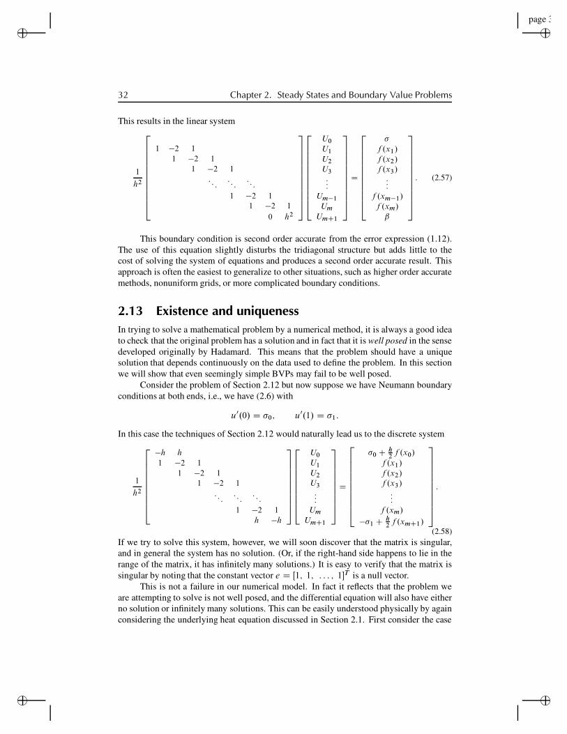
“rjlfdm”2007/6/1page 32✐
✐✐
✐
✐✐
✐✐
32 Chapter 2. Steady States and Boundary Value Problems
This results in the linear system
1
h2
2
666666666664
1 !2 11 !2 1
1 !2 1: : :
: : :: : :
1 !2 11 !2 1
0 h2
3
777777777775
2
666666666664
U0
U1
U2
U3:::
Um!1
Um
UmC1
3
777777777775
D
2
666666666664
!f .x1/f .x2/f .x3/:::
f .xm!1/f .xm/ˇ
3
777777777775
: (2.57)
This boundary condition is second order accurate from the error expression (1.12).The use of this equation slightly disturbs the tridiagonal structure but adds little to thecost of solving the system of equations and produces a second order accurate result. Thisapproach is often the easiest to generalize to other situations, such as higher order accuratemethods, nonuniform grids, or more complicated boundary conditions.
2.13 Existence and uniquenessIn trying to solve a mathematical problem by a numerical method, it is always a good ideato check that the original problem has a solution and in fact that it is well posed in the sensedeveloped originally by Hadamard. This means that the problem should have a uniquesolution that depends continuously on the data used to define the problem. In this sectionwe will show that even seemingly simple BVPs may fail to be well posed.
Consider the problem of Section 2.12 but now suppose we have Neumann boundaryconditions at both ends, i.e., we have (2.6) with
u0.0/ D !0; u0.1/ D !1:
In this case the techniques of Section 2.12 would naturally lead us to the discrete system
1
h2
2
6666666664
!h h1 !2 1
1 !2 11 !2 1
: : :: : :
: : :
1 !2 1h !h
3
7777777775
2
6666666664
U0
U1
U2
U3:::
Um
UmC1
3
7777777775
D
2
66666666664
!0 C h2f .x0/
f .x1/f .x2/f .x3/:::
f .xm/
!!1 C h2f .xmC1/
3
77777777775
:
(2.58)If we try to solve this system, however, we will soon discover that the matrix is singular,and in general the system has no solution. (Or, if the right-hand side happens to lie in therange of the matrix, it has infinitely many solutions.) It is easy to verify that the matrix issingular by noting that the constant vector e D Œ1; 1; : : : ; 1"T is a null vector.
This is not a failure in our numerical model. In fact it reflects that the problem weare attempting to solve is not well posed, and the differential equation will also have eitherno solution or infinitely many solutions. This can be easily understood physically by againconsidering the underlying heat equation discussed in Section 2.1. First consider the case
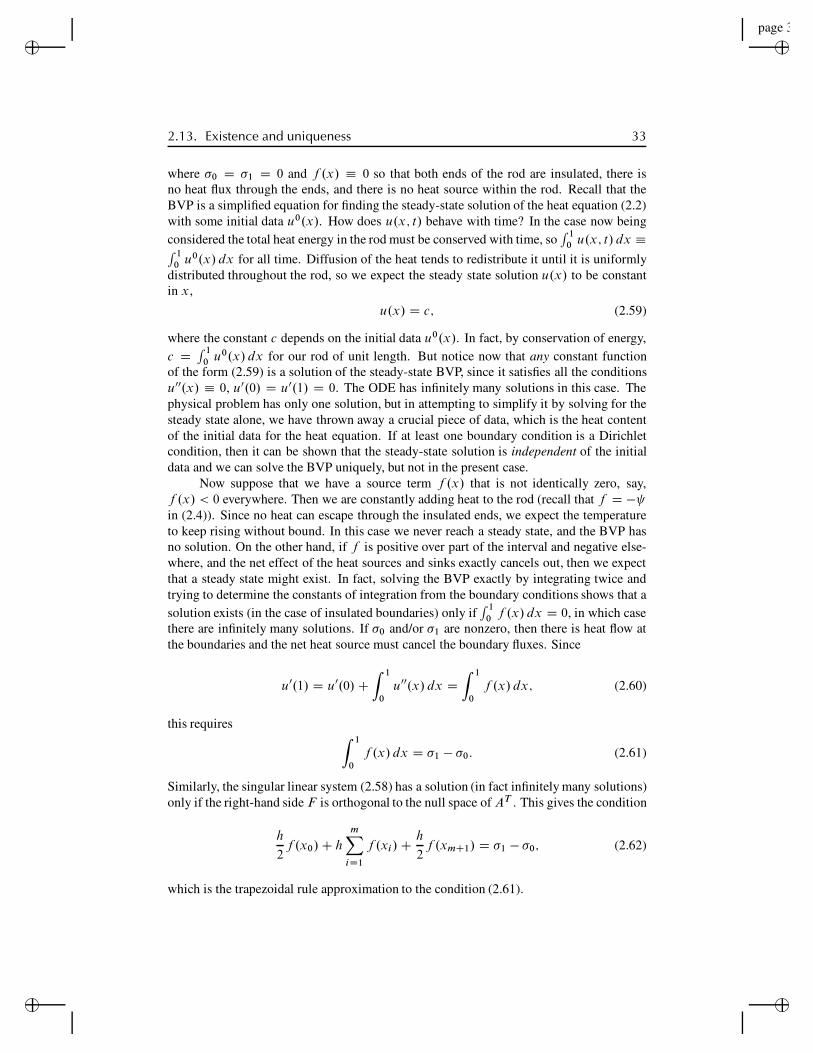
“rjlfdm”2007/6/1page 33✐
✐✐
✐
✐✐
✐✐
2.13. Existence and uniqueness 33
where !0 D !1 D 0 and f .x/ ! 0 so that both ends of the rod are insulated, there isno heat flux through the ends, and there is no heat source within the rod. Recall that theBVP is a simplified equation for finding the steady-state solution of the heat equation (2.2)with some initial data u0.x/. How does u.x; t/ behave with time? In the case now beingconsidered the total heat energy in the rod must be conserved with time, so
R 10 u.x; t/ dx !R 1
0 u0.x/ dx for all time. Diffusion of the heat tends to redistribute it until it is uniformlydistributed throughout the rod, so we expect the steady state solution u.x/ to be constantin x,
u.x/ D c; (2.59)
where the constant c depends on the initial data u0.x/. In fact, by conservation of energy,c D
R 1
0 u0.x/ dx for our rod of unit length. But notice now that any constant functionof the form (2.59) is a solution of the steady-state BVP, since it satisfies all the conditionsu00.x/ ! 0, u0.0/ D u0.1/ D 0. The ODE has infinitely many solutions in this case. Thephysical problem has only one solution, but in attempting to simplify it by solving for thesteady state alone, we have thrown away a crucial piece of data, which is the heat contentof the initial data for the heat equation. If at least one boundary condition is a Dirichletcondition, then it can be shown that the steady-state solution is independent of the initialdata and we can solve the BVP uniquely, but not in the present case.
Now suppose that we have a source term f .x/ that is not identically zero, say,f .x/ < 0 everywhere. Then we are constantly adding heat to the rod (recall that f D " in (2.4)). Since no heat can escape through the insulated ends, we expect the temperatureto keep rising without bound. In this case we never reach a steady state, and the BVP hasno solution. On the other hand, if f is positive over part of the interval and negative else-where, and the net effect of the heat sources and sinks exactly cancels out, then we expectthat a steady state might exist. In fact, solving the BVP exactly by integrating twice andtrying to determine the constants of integration from the boundary conditions shows that asolution exists (in the case of insulated boundaries) only if
R 1
0 f .x/ dx D 0, in which casethere are infinitely many solutions. If !0 and/or !1 are nonzero, then there is heat flow atthe boundaries and the net heat source must cancel the boundary fluxes. Since
u0.1/ D u0.0/CZ 1
0
u00.x/ dx DZ 1
0
f .x/ dx; (2.60)
this requiresZ 1
0
f .x/ dx D !1 " !0: (2.61)
Similarly, the singular linear system (2.58) has a solution (in fact infinitely many solutions)only if the right-hand side F is orthogonal to the null space of AT . This gives the condition
h
2f .x0/C h
mX
iD1
f .xi/C h
2f .xmC1/ D !1 " !0; (2.62)
which is the trapezoidal rule approximation to the condition (2.61).
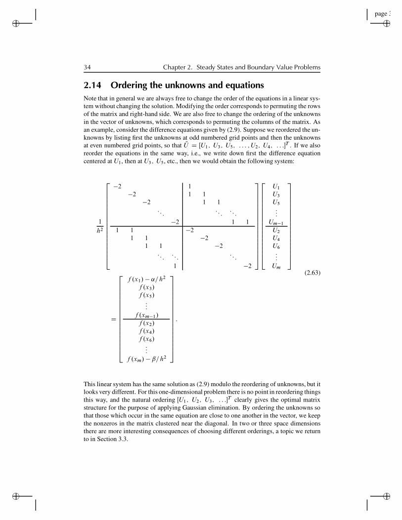
“rjlfdm”2007/6/1page 34✐
✐✐
✐
✐✐
✐✐
34 Chapter 2. Steady States and Boundary Value Problems
2.14 Ordering the unknowns and equationsNote that in general we are always free to change the order of the equations in a linear sys-tem without changing the solution. Modifying the order corresponds to permuting the rowsof the matrix and right-hand side. We are also free to change the ordering of the unknownsin the vector of unknowns, which corresponds to permuting the columns of the matrix. Asan example, consider the difference equations given by (2.9). Suppose we reordered the un-knowns by listing first the unknowns at odd numbered grid points and then the unknownsat even numbered grid points, so that QU D ŒU1; U3; U5; : : : ;U2; U4; : : :!
T . If we alsoreorder the equations in the same way, i.e., we write down first the difference equationcentered at U1, then at U3; U5, etc., then we would obtain the following system:
1
h2
2
66666666666666664
!2 1!2 1 1
!2 1 1: : :
: : :: : :
!2 1 1
1 1 !21 1 !2
1 1 !2: : :
: : :: : :
1 !2
3
77777777777777775
2
66666666666666664
U1
U3
U5
:::Um!1
U2
U4
U6
:::Um
3
77777777777777775
D
2
66666666666666664
f .x1/ ! ˛=h2
f .x3/f .x5/:::
f .xm!1/f .x2/f .x4/f .x6/:::
f .xm/ ! ˇ=h2
3
77777777777777775
:
(2.63)
This linear system has the same solution as (2.9) modulo the reordering of unknowns, but itlooks very different. For this one-dimensional problem there is no point in reordering thingsthis way, and the natural ordering ŒU1; U2; U3; : : :!
T clearly gives the optimal matrixstructure for the purpose of applying Gaussian elimination. By ordering the unknowns sothat those which occur in the same equation are close to one another in the vector, we keepthe nonzeros in the matrix clustered near the diagonal. In two or three space dimensionsthere are more interesting consequences of choosing different orderings, a topic we returnto in Section 3.3.
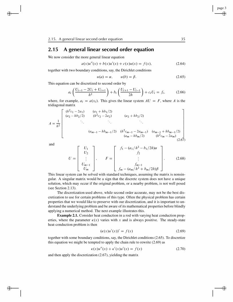
“rjlfdm”2007/6/1page 35✐
✐✐
✐
✐✐
✐✐
2.15. A general linear second order equation 35
2.15 A general linear second order equationWe now consider the more general linear equation
a.x/u00.x/C b.x/u0.x/C c.x/u.x/ D f .x/; (2.64)
together with two boundary conditions, say, the Dirichlet conditions
u.a/ D ˛; u.b/ D ˇ: (2.65)
This equation can be discretized to second order by
ai
!Ui!1 ! 2Ui C UiC1
h2
"C bi
!UiC1 ! Ui!1
2h
"C ciUi D fi ; (2.66)
where, for example, ai D a.xi/. This gives the linear system AU D F , where A is thetridiagonal matrix
A D 1
h2
2
666666664
.h2c1 ! 2a1/ .a1 C hb1=2/
.a2 ! hb2=2/ .h2c2 ! 2a2/ .a2 C hb2=2/
: : :: : :
: : :
.am!1 ! hbm!1=2/ .h2cm!1 ! 2am!1/ .am!1 C hbm!1=2/
.am ! hbm=2/ .h2cm ! 2am/
3
777777775
(2.67)and
U D
2
666664
U1
U2
:::Um!1
Um
3
777775; F D
2
666664
f1 ! .a1=h2 ! b1=2h/˛f2
:::fm!1
fm ! .am=h2 C bm=2h/ˇ
3
777775: (2.68)
This linear system can be solved with standard techniques, assuming the matrix is nonsin-gular. A singular matrix would be a sign that the discrete system does not have a uniquesolution, which may occur if the original problem, or a nearby problem, is not well posed(see Section 2.13).
The discretization used above, while second order accurate, may not be the best dis-cretization to use for certain problems of this type. Often the physical problem has certainproperties that we would like to preserve with our discretization, and it is important to un-derstand the underlying problem and be aware of its mathematical properties before blindlyapplying a numerical method. The next example illustrates this.
Example 2.1. Consider heat conduction in a rod with varying heat conduction prop-erties, where the parameter !.x/ varies with x and is always positive. The steady-stateheat-conduction problem is then
.!.x/u0.x//0 D f .x/ (2.69)
together with some boundary conditions, say, the Dirichlet conditions (2.65). To discretizethis equation we might be tempted to apply the chain rule to rewrite (2.69) as
!.x/u00.x/C !0.x/u0.x/ D f .x/ (2.70)
and then apply the discretization (2.67), yielding the matrix

“rjlfdm”2007/6/1page 36✐
✐✐
✐
✐✐
✐✐
36 Chapter 2. Steady States and Boundary Value Problems
A D 1
h2
2
66666664
!2!1 .!1 C h!01=2/
.!2 ! h!02=2/ !2!2 .!2 C h!0
2=2/
: : :: : :
: : :
.!m!1 ! h!0m!1
=2/ !2!m!1 .!m!1 C h!0m!1
=2/
.!m ! h!0m=2/ !2!m
3
77777775
:
(2.71)However, this is not the best approach. It is better to discretize the physical problem (2.69)directly. This can be done by first approximating !.x/u0.x/ at points halfway between thegrid points, using a centered approximation
!.xiC1=2/u0.xiC1=2/ D !iC1=2
!UiC1 ! Ui
h
"
and the analogous approximation at xi!1=2. Differencing these then gives a centered ap-proximation to .!u0/0 at the grid point xi:
.!u0/0.xi/ "1
h
#!iC1=2
!UiC1 ! Ui
h
"! !i!1=2
!Ui ! Ui!1
h
"$
D 1
h2Œ!i!1=2Ui!1 ! .!i!1=2 C !iC1=2/Ui C !iC1=2UiC1":
(2.72)
This leads to the matrix
A D 1
h2
2
66666664
!.!1=2 C !3=2/ !3=2
!3=2 !.!3=2 C !5=2/ !5=2
: : :: : :
: : :
!m!3=2 !.!m!3=2 C !m!1=2/ !m!1=2
!m!1=2 !.!m!1=2 C !mC1=2/
3
77777775
:
(2.73)Comparing (2.71) to (2.73), we see that they agree to O.h2/, noting, for example, that
!.xiC1=2/ D !.xi /C 1
2h!0.xi/C O.h2/ D !.xiC1/ !
1
2h!0.xiC1/C O.h2/:
However, the matrix (2.73) has the advantage of being symmetric, as we would hope, sincethe original differential equation is self-adjoint. Moreover, since ! > 0, the matrix can beshown to be nonsingular and negative definite. This means that all the eigenvalues are neg-ative, a property also shared by the differential operator @
@x!.x/@
@x (see Section C.8). It isgenerally desirable to have important properties such as these modeled by the discrete ap-proximation to the differential equation. One can then show, for example, that the solutionto the difference equations satisfies a maximum principle of the same type as the solutionto the differential equation: for the homogeneous equation with f .x/ # 0, the values ofu.x/ lie between the values of the boundary values ˛ and ˇ everywhere, so the maximumand minimum values of u arise on the boundaries. For the heat conduction problem this isphysically obvious: the steady-state temperature in the rod won’t exceed what’s imposedat the boundaries if there is no heat source.

“rjlfdm”2007/6/1page 37✐
✐✐
✐
✐✐
✐✐
2.16. Nonlinear equations 37
When solving the resulting linear system by iterative methods (see Chapters 3 and 4)it is also often desirable that the matrix have properties such as negative definiteness, sincesome iterative methods (e.g., the conjugate-gradient (CG) method in Section 4.3) dependon such properties.
2.16 Nonlinear equationsWe next consider a nonlinear BVP to illustrate the new complications that arise in thiscase. We will consider a specific example that has a simple physical interpretation whichmakes it easy to understand and interpret solutions. This example also illustrates that notall 2-point BVPs are steady-state problems.
Consider the motion of a pendulum with mass m at the end of a rigid (but massless)bar of length L, and let !.t/ be the angle of the pendulum from vertical at time t , as illus-trated in Figure 2.3. Ignoring the mass of the bar and forces of friction and air resistance,we see that the differential equation for the pendulum motion can be well approximated by
! 00.t/ D !.g=L/ sin.!.t//; (2.74)
where g is the gravitational constant. Taking g=L D 1 for simplicity we have
! 00.t/ D ! sin.!.t// (2.75)
as our model problem.For small amplitudes of the angle ! it is possible to approximate sin.!/ " ! and
obtain the approximate linear differential equation
! 00.t/ D !!.t/ (2.76)
(a)
!
0 1 2 3 4 5 6 7 8 9 10−2
−1
0
1
2
0 1 2 3 4 5 6 7 8 9 10−2
−1
0
1
2
(b)
(c)
Figure 2.3. (a) Pendulum. (b) Solutions to the linear equation (2.76) for variousinitial ! and zero initial velocity. (c) Solutions to the nonlinear equation (2.75) for variousinitial ! and zero initial velocity.

“rjlfdm”2007/6/1page 38✐
✐✐
✐
✐✐
✐✐
38 Chapter 2. Steady States and Boundary Value Problems
with general solutions of the form A cos.t/ C B sin.t/. The motion of a pendulum that isoscillating only a small amount about the equilibrium at ! D 0 can be well approximatedby this sinusoidal motion, which has period 2" independent of the amplitude. For larger-amplitude motions, however, solving (2.76) does not give good approximations to the truebehavior. Figures 2.3(b) and (c) show some sample solutions to the two equations.
To fully describe the problem we also need to specify two auxiliary conditions inaddition to the second order differential equation (2.75). For the pendulum problem theIVP is most natural—we set the pendulum swinging from some initial position !.0/ withsome initial angular velocity ! 0.0/, which gives two initial conditions that are enough todetermine a unique solution at all later times.
To obtain instead a BVP, consider the situation in which we wish to set the pendulumswinging from some initial given location !.0/ D ˛ with some unknown angular velocity! 0.0/ in such a way that the pendulum will be at the desired location !.T / D ˇ at somespecified later time T . Then we have a 2-point BVP
! 00.t/ D ! sin.!.t// for 0 < t < T;
!.0/ D ˛; !.T / D ˇ:(2.77)
Similar BVPs do arise in more practical situations, for example, trying to shoot a missilein such a way that it hits a desired target. In fact, this latter example gives rise to the nameshooting method for another approach to solving 2-point BVPs that is discussed in [4] and[54], for example.
2.16.1 Discretization of the nonlinear boundary value problemWe can discretize the nonlinear problem (2.75) in the obvious manner, following our ap-proach for linear problems, to obtain the system of equations
1
h2.!i!1 ! 2!i C !iC1/C sin.!i / D 0 (2.78)
for i D 1; 2; : : : ; m, where h D T=.m C 1/ and we set !0 D ˛ and !mC1 D ˇ. As inthe linear case, we have a system of m equations for m unknowns. However, this is now anonlinear system of equations of the form
G.!/ D 0; (2.79)
where G W Rm ! Rm. This cannot be solved as easily as the tridiagonal linear systemsencountered so far. Instead of a direct method we must generally use some iterative method,such as Newton’s method. If ! Œk! is our approximation to ! in step k , then Newton’s methodis derived via the Taylor series expansion
G.! ŒkC1!/ D G.! Œk!/C G0.! Œk!/.! ŒkC1! ! ! Œk!/C " " " :
Setting G.! ŒkC1!/ D 0 as desired, and dropping the higher order terms, results in
0 D G.! Œk!/C G0.! Œk!/.! ŒkC1! ! ! Œk!/:
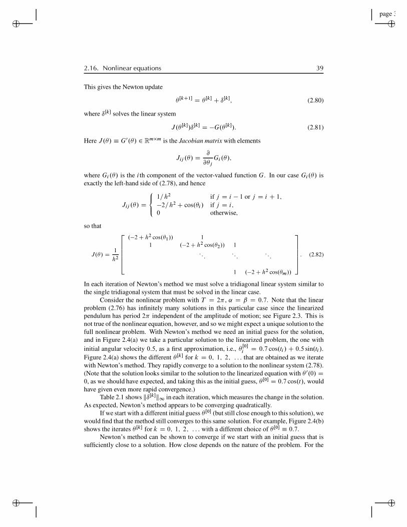
“rjlfdm”2007/6/1page 39✐
✐✐
✐
✐✐
✐✐
2.16. Nonlinear equations 39
This gives the Newton update
! ŒkC1! D ! Œk! C ıŒk!; (2.80)
where ıŒk! solves the linear system
J.! Œk!/ıŒk! D !G.! Œk!/: (2.81)
Here J.!/ " G0.!/ 2 Rm!m is the Jacobian matrix with elements
Jij .!/ D @
@!jGi .!/;
where Gi .!/ is the i th component of the vector-valued function G. In our case Gi.!/ isexactly the left-hand side of (2.78), and hence
Jij .!/ D
8<
:
1=h2 if j D i ! 1 or j D i C 1;
!2=h2 C cos.!i / if j D i;0 otherwise;
so that
J.!/ D 1
h2
2
666664
.!2 C h2 cos.!1// 1
1 .!2 C h2 cos.!2// 1
: : :: : :
: : :
1 .!2 C h2 cos.!m//
3
777775: (2.82)
In each iteration of Newton’s method we must solve a tridiagonal linear system similar tothe single tridiagonal system that must be solved in the linear case.
Consider the nonlinear problem with T D 2" , ˛ D ˇ D 0:7. Note that the linearproblem (2.76) has infinitely many solutions in this particular case since the linearizedpendulum has period 2" independent of the amplitude of motion; see Figure 2.3. This isnot true of the nonlinear equation, however, and so we might expect a unique solution to thefull nonlinear problem. With Newton’s method we need an initial guess for the solution,and in Figure 2.4(a) we take a particular solution to the linearized problem, the one withinitial angular velocity 0:5, as a first approximation, i.e., ! Œ0!
i D 0:7 cos.ti / C 0:5 sin.ti /.Figure 2.4(a) shows the different ! Œk! for k D 0; 1; 2; : : : that are obtained as we iteratewith Newton’s method. They rapidly converge to a solution to the nonlinear system (2.78).(Note that the solution looks similar to the solution to the linearized equation with ! 0.0/ D0, as we should have expected, and taking this as the initial guess, ! Œ0! D 0:7 cos.t/, wouldhave given even more rapid convergence.)
Table 2.1 shows kıŒk!k1 in each iteration, which measures the change in the solution.As expected, Newton’s method appears to be converging quadratically.
If we start with a different initial guess ! Œ0! (but still close enough to this solution), wewould find that the method still converges to this same solution. For example, Figure 2.4(b)shows the iterates ! Œk! for k D 0; 1; 2; : : : with a different choice of ! Œ0! " 0:7.
Newton’s method can be shown to converge if we start with an initial guess that issufficiently close to a solution. How close depends on the nature of the problem. For the

“rjlfdm”2007/6/1page 40✐
✐✐
✐
✐✐
✐✐
40 Chapter 2. Steady States and Boundary Value Problems
(a) 0 1 2 3 4 5 6 7
−1
−0.8
−0.6
−0.4
−0.2
0
0.2
0.4
0.6
0.8
1
0
1
23,4
(b) 0 1 2 3 4 5 6 7
−1
−0.8
−0.6
−0.4
−0.2
0
0.2
0.4
0.6
0.8
1
0
1
2
3,4
Figure 2.4. Convergence of Newton iterates toward a solution of the pendulumproblem. The iterates ! Œk! for k D 1; 2; : : : are denoted by the number k in the plots. (a)Starting from !
Œ0!i D 0:7 cos.ti /C 0:5 sin.ti /. (b) Starting from !
Œ0!i D 0:7.
Table 2.1. Change kıŒk!k1 in solution in each iteration of Newton’s method.
k Figure 2.4(a) Figure 2.5
0 3.2841e!01 4.2047e+001 1.7518e!01 5.3899e+002 3.1045e!02 8.1993e+003 2.3739e!04 7.7111e!014 1.5287e!08 3.8154e!025 5.8197e!15 2.2490e!046 1.5856e!15 9.1667e!097 1.3395e!15
problem considered above one need not start very close to the solution to converge, as seenin the examples, but for more sensitive problems one might have to start extremely close.In such cases it may be necessary to use a technique such as continuation to find suitableinitial data; see Section 2.19.
2.16.2 NonuniquenessThe nonlinear problem does not have an infinite family of solutions the way the linearequation does on the interval Œ0; 2"#, and the solution found above is an isolated solution inthe sense that there are no other solutions very nearby (it is also said to be locally unique).However, it does not follow that this is the unique solution to the BVP (2.77). In fact phys-ically we should expect other solutions. The solution we found corresponds to releasingthe pendulum with nearly zero initial velocity. It swings through nearly one complete cycleand returns to the initial position at time T .
Another possibility would be to propel the pendulum upward so that it rises towardthe top (an unstable equilibrium) at ! D " , before falling back down. By specifying thecorrect velocity we should be able to arrange it so that the pendulum falls back to ! D 0:7again at T D 2" . In fact it is possible to find such a solution for any T > 0.
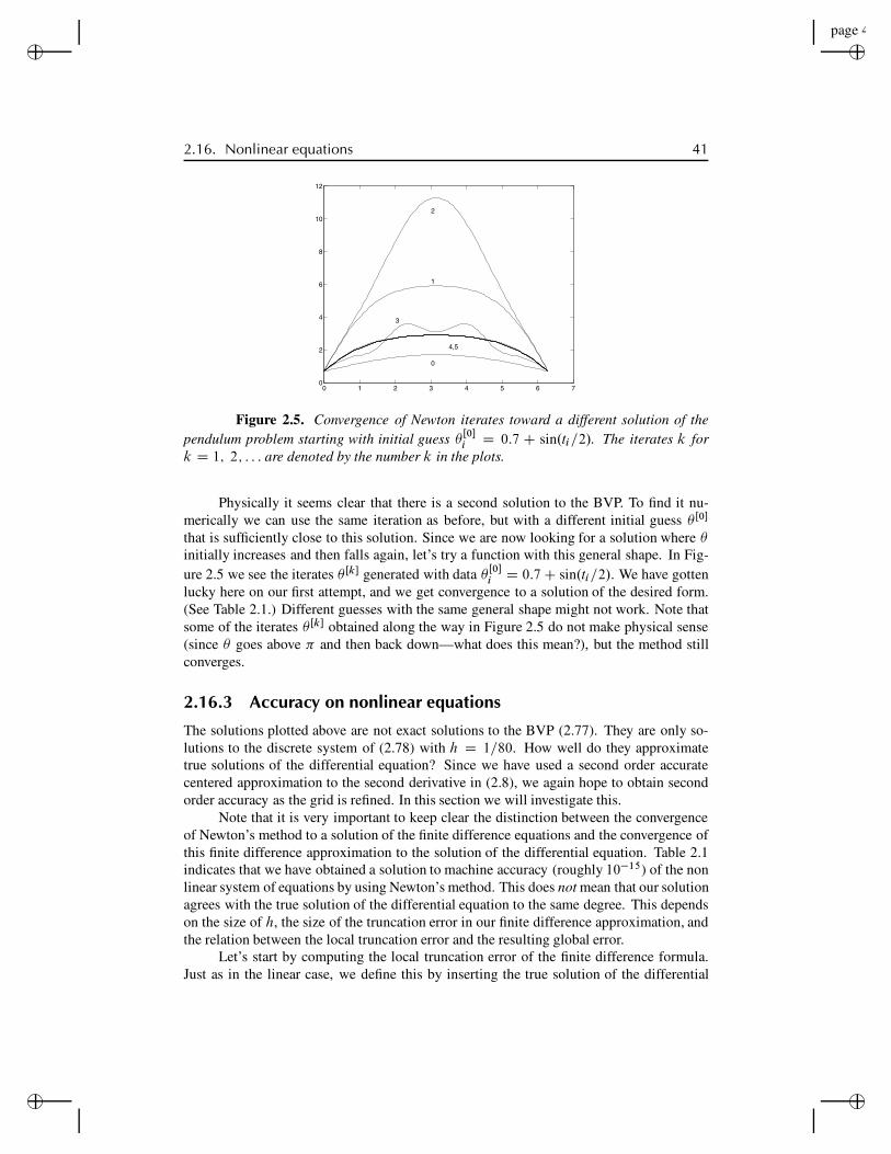
“rjlfdm”2007/6/1page 41✐
✐✐
✐
✐✐
✐✐
2.16. Nonlinear equations 41
0 1 2 3 4 5 6 70
2
4
6
8
10
12
0
1
2
3
4,5
Figure 2.5. Convergence of Newton iterates toward a different solution of thependulum problem starting with initial guess ! Œ0!
i D 0:7 C sin.ti=2/. The iterates k fork D 1; 2; : : : are denoted by the number k in the plots.
Physically it seems clear that there is a second solution to the BVP. To find it nu-merically we can use the same iteration as before, but with a different initial guess ! Œ0!
that is sufficiently close to this solution. Since we are now looking for a solution where !initially increases and then falls again, let’s try a function with this general shape. In Fig-ure 2.5 we see the iterates ! Œk! generated with data ! Œ0!
i D 0:7 C sin.ti=2/. We have gottenlucky here on our first attempt, and we get convergence to a solution of the desired form.(See Table 2.1.) Different guesses with the same general shape might not work. Note thatsome of the iterates ! Œk! obtained along the way in Figure 2.5 do not make physical sense(since ! goes above " and then back down—what does this mean?), but the method stillconverges.
2.16.3 Accuracy on nonlinear equationsThe solutions plotted above are not exact solutions to the BVP (2.77). They are only so-lutions to the discrete system of (2.78) with h D 1=80. How well do they approximatetrue solutions of the differential equation? Since we have used a second order accuratecentered approximation to the second derivative in (2.8), we again hope to obtain secondorder accuracy as the grid is refined. In this section we will investigate this.
Note that it is very important to keep clear the distinction between the convergenceof Newton’s method to a solution of the finite difference equations and the convergence ofthis finite difference approximation to the solution of the differential equation. Table 2.1indicates that we have obtained a solution to machine accuracy (roughly 10!15) of the nonlinear system of equations by using Newton’s method. This does not mean that our solutionagrees with the true solution of the differential equation to the same degree. This dependson the size of h, the size of the truncation error in our finite difference approximation, andthe relation between the local truncation error and the resulting global error.
Let’s start by computing the local truncation error of the finite difference formula.Just as in the linear case, we define this by inserting the true solution of the differential
“rjlfdm”2007/6/1page 42✐
✐✐
✐
✐✐
✐✐
42 Chapter 2. Steady States and Boundary Value Problems
equation into the finite difference equations. This will not satisfy the equations exactly, andthe residual is what we call the local truncation error (LTE):
!i D 1
h2.".ti!1/ ! 2".ti /C ".tiC1//C sin.".ti //
D ." 00.ti /C sin.".ti /// C 1
12h2" 0000.ti /C O.h4/
D 1
12h2" 0000.ti /C O.h4/:
(2.83)
Note that we have used the differential equation to set " 00.ti /C sin.".ti // D 0, which holdsexactly since ".t/ is the exact solution. The LTE is O.h2/ and has exactly the same formas in the linear case. (For a more complicated nonlinear problem it might not work out sosimply, but similar expressions result.) The vector ! with components !i is simply G. O"/,where O" is the vector made up of the true solution at each grid point. We now want toobtain an estimate on the global error E based on this local error. We can attempt to followthe path used in Section 2.6 for linear problems. We have
G."/ D 0;
G. O"/ D !;
and subtracting givesG."/ ! G. O"/ D !!: (2.84)
We would like to derive from this a relation for the global error E D "! O" . If G were linear(say, G."/ D A" ! F ), we would have G."/ ! G. O" / D A" ! A O" D A." ! O"/ D AE,giving an expression in terms of the global error E D " ! O" . This is what we used inSection 2.7.
In the nonlinear case we cannot express G."/ ! G. O" / directly in terms of " ! O" .However, we can use Taylor series expansions to write
G."/ D G. O"/C J. O"/E C O.kEk2/;
where J. O"/ is again the Jacobian matrix of the difference formulas, evaluated now at theexact solution. Combining this with (2.84) gives
J. O"/E D !! C O.kEk2/:
If we ignore the higher order terms, then we again have a linear relation between the localand global errors.
This motivates the following definition of stability. Here we let OJ h denote the Ja-cobian matrix of the difference formulas evaluated at the true solution on a grid with gridspacing h.
Definition 2.2. The nonlinear difference method G."/ D 0 is stable in some norm k"k if thematrices . OJ h/!1 are uniformly bounded in this norm as h ! 0, i.e., there exist constantsC and h0 such that
k. OJ h/!1k # C for all h < h0: (2.85)

“rjlfdm”2007/6/1page 43✐
✐✐
✐
✐✐
✐✐
2.17. Singular perturbations and boundary layers 43
It can be shown that if the method is stable in this sense, and consistent in this norm(k!hk ! 0), then the method converges and kEhk ! 0 as h ! 0. This is not obviousin the nonlinear case: we obtain a linear system for E only by dropping the O.kEk2/nonlinear terms. Since we are trying to show that E is small, we can’t necessarily assumethat these terms are negligible in the course of the proof, at least not without some care.See [54] for a proof.
It makes sense that it is uniform boundedness of the inverse Jacobian at the exactsolution that is required for stability. After all, it is essentially this Jacobian matrix that isused in solving linear systems in the course of Newton’s method, once we get very close tothe solution.
Warning: We state a final reminder that there is a difference between convergenceof the difference method as h ! 0 and convergence of Newton’s method, or some otheriterative method, to the solution of the difference equations for some particular h. Stabilityof the difference method does not imply that Newton’s method will converge from a poorinitial guess. It can be shown, however, that with a stable method, Newton’s method willconverge from a sufficiently good initial guess; see [54]. Also, the fact that Newton’smethod has converged to a solution of the nonlinear system of difference equations, with anerror of 10!15, say, does not mean that we have a good solution to the original differentialequation. The global error of the difference equations determines this.
2.17 Singular perturbations and boundary layersIn this section we consider some singular perturbation problems to illustrate the difficultiesthat can arise when numerically solving problems with boundary layers or other regionswhere the solution varies rapidly. See [55], [56] for more detailed discussions of singularperturbation problems. In particular, the example used here is very similar to one that canbe found in [55], where solution by matched asymptotic expansions is discussed.
As a simple example we consider a steady-state advection-diffusion equation. Thetime-dependent equation has the form
ut C aux D "uxx C (2.86)
in the simplest case. This models the temperature u.x; t/ of a fluid flowing through a pipewith constant velocity a, where the fluid has constant heat diffusion coefficient " and isa source term from heating through the walls of the tube.
If a > 0, then we naturally have a boundary condition at the left boundary (say,x D 0),
u.0; t/ D ˛.t/;
specifying the temperature of the incoming fluid. At the right boundary (say, x D 1) thefluid is flowing out and so it may seem that the temperature is determined only by whatis happening in the pipe, and no boundary condition is needed here. This is correct if" D 0 since the first order advection equation needs only one boundary condition and weare allowed to specify u only at the left boundary. However, if " > 0, then heat can diffuseupstream, and we need to also specify u.1; t/ D ˇ.t/ to determine a unique solution.
If ˛; ˇ, and are all independent of t , then we expect a steady-state solution, whichwe hope to find by solving the linear 2-point boundary value problem
“rjlfdm”2007/6/1page 44✐
✐✐
✐
✐✐
✐✐
44 Chapter 2. Steady States and Boundary Value Problems
au0.x/ D !u00.x/C .x/;
u.0/ D ˛; u.1/ D ˇ:(2.87)
This can be discretized using the approach of Section 2.4. If a is small relative to !, thenthis problem is easy to solve. In fact for a D 0 this is just the steady-state heat equationdiscussed in Section 2.15, and for small a the solution appears nearly identical.
But now suppose a is large relative to ! (i.e., we crank up the velocity, or we decreasethe ability of heat to diffuse with the velocity a > 0 fixed). More properly we shouldwork in terms of the nondimensional Peclet number, which measures the ratio of advectionvelocity to transport speed due to diffusion. Here we introduce a parameter " which is likethe inverse of the Peclet number, " D !=a, and rewrite (2.87) in the form
"u00.x/ ! u0.x/ D f .x/: (2.88)
Then taking a large relative to ! (large Peclet number) corresponds to the case " " 1.We should expect difficulties physically in this case where advection overwhelms
diffusion. It would be very difficult to maintain a fixed temperature at the outflow endof the tube in this situation. If we had a thermal device that was capable of doing so byinstantaneously heating the fluid to the desired temperature as it passes the right boundary,independent of the temperature of the fluid flowing toward this point, then we would expectthe temperature distribution to be essentially discontinuous at this boundary.
Mathematically we expect trouble as " ! 0 because in the limit " D 0 the equation(2.88) reduces to a first order equation (the steady advection equation)
!u0.x/ D f .x/; (2.89)
which allows only one boundary condition, rather than two. For " > 0, no matter howsmall, we have a second order equation that needs two conditions, but we expect to perhapssee strange behavior at the outflow boundary as " ! 0, since in the limit we are overspecifying the problem.
Figure 2.6(a) shows how solutions to (2.88) appear for various values of " in the case˛ D 1, ˇ D 3, and f .x/ D !1. In this case the exact solution is
u.x/ D ˛ C x C .ˇ ! ˛ ! 1/
ex=! ! 1
e1=! ! 1
!: (2.90)
Note that as " ! 0 the solution tends toward a discontinuous function that jumps to thevalue ˇ at the last possible moment. This region of rapid transition is called the boundarylayer and it can be shown that for this problem the width of this layer is O."/ as " ! 0.
The equation (2.87) with 0 < " " 1 is called a singularly perturbed equation. It isa small perturbation of (2.89), but this small perturbation completely changes the characterof the equation (from a first order to a second order equation). Typically any differen-tial equation having a small parameter multiplying the highest order derivative will give asingular perturbation problem.
By contrast, going from the pure diffusion equation !uxx D f to an advectiondiffusion equation !uxx ! aux D f for very small a is a regular perturbation. Bothof these equations are second order differential equations requiring the same number of
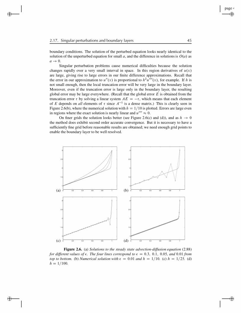
“rjlfdm”2007/6/1page 45✐
✐✐
✐
✐✐
✐✐
2.17. Singular perturbations and boundary layers 45
boundary conditions. The solution of the perturbed equation looks nearly identical to thesolution of the unperturbed equation for small a, and the difference in solutions is O.a/ asa ! 0.
Singular perturbation problems cause numerical difficulties because the solutionchanges rapidly over a very small interval in space. In this region derivatives of u.x/are large, giving rise to large errors in our finite difference approximations. Recall thatthe error in our approximation to u00.x/ is proportional to h2u0000.x/, for example. If h isnot small enough, then the local truncation error will be very large in the boundary layer.Moreover, even if the truncation error is large only in the boundary layer, the resultingglobal error may be large everywhere. (Recall that the global error E is obtained from thetruncation error ! by solving a linear system AE D !! , which means that each elementof E depends on all elements of ! since A!1 is a dense matrix.) This is clearly seen inFigure 2.6(b), where the numerical solution with h D 1=10 is plotted. Errors are large evenin regions where the exact solution is nearly linear and u0000 " 0.
On finer grids the solution looks better (see Figure 2.6(c) and (d)), and as h ! 0the method does exhibit second order accurate convergence. But it is necessary to have asufficiently fine grid before reasonable results are obtained; we need enough grid points toenable the boundary layer to be well resolved.
(a) 0 0.2 0.4 0.6 0.8 1
1
1.5
2
2.5
3
(b) 0 0.2 0.4 0.6 0.8 1
1
1.5
2
2.5
3
(c) 0 0.2 0.4 0.6 0.8 1
1
1.5
2
2.5
3
(d) 0 0.2 0.4 0.6 0.8 1
1
1.5
2
2.5
3
Figure 2.6. (a) Solutions to the steady state advection-diffusion equation (2.88)for different values of ". The four lines correspond to " D 0:3; 0:1; 0:05, and 0:01 fromtop to bottom. (b) Numerical solution with " D 0:01 and h D 1=10. (c) h D 1=25. (d)h D 1=100.
“rjlfdm”2007/6/1page 46✐
✐✐
✐
✐✐
✐✐
46 Chapter 2. Steady States and Boundary Value Problems
2.17.1 Interior layersThe above example has a boundary layer, a region of rapid transition at one boundary. Otherproblems may have interior layers instead. In this case the solution is smooth except forsome thin region interior to the interval where a rapid transition occurs. Such problems canbe even more difficult to solve since we often don’t know a priori where the interior layerwill be. Perturbation theory can often be used to analyze singular perturbation problemsand predict where the layers will occur, how wide they will be (as a function of the smallparameter !), and how the solution behaves. The use of perturbation theory to obtain goodapproximations to problems of this type is a central theme of classical applied mathematics.
These analytic techniques can often be used to good advantage along with numericalmethods, for example, to obtain a good initial guess for Newton’s method, or to choose anappropriate nonuniform grid as discussed in the next section. In some cases it is possibleto develop special numerical methods that have the correct singular behavior built into theapproximation in such a way that far better accuracy is achieved than with a naive numericalmethod.
Example 2.2. Consider the nonlinear boundary value problem
!u00 C u.u0 ! 1/ D 0 for a " x " b;
u.a/ D ˛; u.b/ D ˇ:(2.91)
For small ! this is a singular perturbation problem since ! multiplies the highest orderderivative. Setting ! D 0 gives a reduced equation
u.u0 ! 1/ D 0 (2.92)
for which we generally can enforce only one boundary condition. Solutions to (2.92) areu.x/ # 0 or u.x/ D x C C for some constant C . If the boundary condition imposed atx D a or x D b is nonzero, then the solution has the latter form and is either
u.x/ D x C ˛ ! a if u.a/ D ˛ is imposed (2.93)
oru.x/ D x C ˇ ! b if u.b/ D ˇ is imposed: (2.94)
These two solutions are shown in Figure 2.7.For 0 < ! $ 1, the full equation (2.91) has a solution that satisfies both bound-
ary conditions, and Figure 2.7 also shows such a solution. Over most of the domain thesolution is smooth and u00 is small, in which case !u00 is negligible and the solution mustnearly satisfy (2.92). Thus over most of the domain the solution follows one of the linearsolutions to the reduced equation. Both boundary conditions can be satisfied by followingone solution (2.93) near x D a and the other solution (2.94) near x D b. Connecting thesetwo smooth portions of the solution is a narrow zone (the interior solution) where u.x/ israpidly varying. In this layer u00 is very large and the !u00 term of (2.91) is not negligible,and hence u.u0 ! 1/ may be far from zero in this region.
To determine the location and width of the interior layer, and the approximate formof the solution in this layer, we can use perturbation theory. Focusing attention on this

“rjlfdm”2007/6/1page 47✐
✐✐
✐
✐✐
✐✐
2.17. Singular perturbations and boundary layers 47
0 0.2 0.4 0.6 0.8 1−1
−0.5
0
0.5
1
1.5
u.x/
x C ˛ ! a
x C ˇ ! b
Figure 2.7. Outer solutions and full solution to the singular perturbation problemwith a D 0; b D 1, ˛ D !1, and ˇ D 1:5. The solution has an interior layer centeredabout Nx D 0:25.
layer, which we now assume is centered at some location x D Nx, we can zoom in on thesolution by assuming that u.x/ has the approximate form
u.x/ D W ..x ! Nx/=!k/ (2.95)
for some power k to be determined. We are zooming in on a layer of width O.!k / asymp-totically, so determining k will tell us how wide the layer is. From (2.95) we compute
u0.x/ D !!k W 0..x ! Nx/=!k/;
u00.x/ D !!2k W 0..x ! Nx/=!k/:(2.96)
Inserting these expressions in (2.91) gives
! " !!2k W 00."/C W ."/.!!k W 0."/ ! 1/ D 0;
where " D .x ! Nx/=!k . Multiply by !2k!1 to obtain
W 00."/C W ."/.!k!1W 0."/ ! !2k!1/ D 0: (2.97)
By rescaling the independent variable by a factor !k , we have converted the singular pertur-bation problem (2.91) into a problem where the highest order derivative W 00 has coefficient1 and the small parameter appears only in the lower order term. However, the lower orderterm behaves well in the limit ! ! 0 only if we take k # 1. For smaller values of k(zooming in on too large a region asymptotically), the lower order term blows up as ! ! 0,or dividing by !k!1 shows that we still have a singular perturbation problem. This gives ussome information on k .
If we fix x at any value away from Nx, then " ! ˙1 as ! ! 0. So the boundaryvalue problem (2.97) for W ."/ has boundary conditions at ˙1,
W ."/ ! Nx C ˛ ! a as " ! !1;
W ."/ ! Nx C ˇ ! b as " ! C1:(2.98)

“rjlfdm”2007/6/1page 48✐
✐✐
✐
✐✐
✐✐
48 Chapter 2. Steady States and Boundary Value Problems
The “inner solution” W .!/ will then match up with the “outer solutions” given by (2.93)and (2.94) at the edges of the layer. We also require
W 0.!/ ! 0 as ! ! ˙1 (2.99)
since outside the layer the linear functions (2.93) and (2.94) have the desired slope.For (2.97) to give a reasonable 2-point boundary value problem with these three
boundary conditions (2.98) and (2.99), we must take k D 1. We already saw that we needk ! 1, but we also cannot take k > 1 since in this case the lower order term in (2.97)vanishes as " ! 0 and the equation reduces to W 00.!/ D 0. In this case we are zoomingin too far on the solution near x D Nx and the solution simply appears linear, as does anysufficiently smooth function if we zoom in on its behavior at a fixed point. While this doesreveal the behavior extremely close to Nx, it does not allow us to capture the full behavior inthe interior layer. We cannot satisfy all four boundary conditions on W with a solution toW 00.x/ D 0.
Taking k D 1 gives the proper interior problem, and (2.97) becomes
W 00.!/C W .!/.W 0.!/ " "/ D 0: (2.100)
Now letting " ! 0 we obtain
W 00.!/C W .!/W 0.!/ D 0: (2.101)
This equation has solutions of the form
W .!/ D w0 tanh.w0!=2/ (2.102)
for arbitrary constants w0. The boundary conditions (2.98) lead to
w0 D 1
2.a " b C ˇ " ˛/ (2.103)
and
Nx D 1
2.a C b " ˛ " ˇ/: (2.104)
To match this solution to the outer solutions, we require a < Nx < b. If the value ofNx determined by (2.104) doesn’t satisfy this condition, then the original problem has aboundary layer at x D a (if Nx # a) or at x D b (if Nx ! b) instead of an interior layer. Forthe remainder of this discussion we assume a < Nx < b.
We can combine the inner and outer solutions to obtain an approximate solution ofthe form
u.x/ $ Qu.x/ % x " Nx Cw0 tanh.w0.x " Nx/=2"/: (2.105)
Singular perturbation analysis has given us a great deal of information about the so-lution to the problem (2.91). We know that the solution has an interior layer of width O."/at x D Nx with roughly linear solution (2.93), (2.94) outside the layer. This type of infor-mation may be all we need to know about the solution for some applications. If we wantto determine a more detailed numerical approximation to the full solution, this analytical

“rjlfdm”2007/6/1page 49✐
✐✐
✐
✐✐
✐✐
2.18. Nonuniform grids 49
information can be helpful in devising an accurate and efficient numerical method, as wenow consider.
The problem (2.91) can be solved numerically on a uniform grid using the finitedifference equations
Gi.U / ! !
!Ui!1 " 2Ui C UiC1
h2
"C Ui
!UiC1 " Ui!1
2h" 1
"D 0 (2.106)
for i D 1; 2; : : : ; m with U0 D ˛ and UmC1 D ˇ (where, as usual, h D .b"a/=.mC1/).This gives a nonlinear system of equations G.U / D 0 that can be solved using Newton’smethod as described in Section 2.16.1. One way to use the singular perturbation approxi-mation is to generate a good initial guess for Newton’s method, e.g.,
Ui D Qu.xi/; (2.107)
where Qu.x/ is the approximate solution from (2.105). We then have an initial guess that isalready very accurate at nearly all grid points. Newton’s method converges rapidly fromsuch a guess. If the grid is fine enough that the interior layer is well resolved, then a goodapproximation to the full solution is easily obtained. By contrast, starting with a more naiveinitial guess such as Ui D ˛C .x " a/.ˇ " ˛/=.b " a/ leads to nonconvergence when ! issmall.
When ! is very small, highly accurate numerical results can be obtained with lesscomputation by using a nonuniform grid, with grid points clustered in the layer. To con-struct such a grid we can use the singular perturbation analysis to tell us where the pointsshould be clustered (near Nx) and how wide to make the clustering zone. The width of thelayer is O.!/ and, moreover, from (2.102) we expect that most of the transition occurs for,say, j 1
2w0"j < 2. This translates into
jx " Nxj < 4!=w0; (2.108)
where w0 is given by (2.103). The construction and use of nonuniform grids is pursuedfurther in the next section.
2.18 Nonuniform gridsFrom Figure 2.6 it is clear that we need to choose our grid to be fine enough so that severalpoints are within the boundary layer and we can obtain a reasonable solution. If we wantedhigh accuracy within the boundary layer we would have to choose a much finer grid thanshown in this figure. With a uniform grid this means using a very large number of gridpoints, the vast majority of which are in the region where the solution is very smooth andcould be represented well with far fewer points. This waste of effort may be tolerablefor simple one-dimensional problems but can easily be intolerable for more complicatedproblems, particularly in more than one dimension.
Instead it is preferable to use a nonuniform grid for such calculations, with grid pointsclustered in regions where they are most needed. This requires using formulas that aresufficiently accurate on nonuniform grids. For example, a four-point stencil can be usedto obtain second order accuracy for the second derivative operator. Using this for a linear

“rjlfdm”2007/6/1page 50✐
✐✐
✐
✐✐
✐✐
50 Chapter 2. Steady States and Boundary Value Problems
problem would give a banded matrix with four nonzero diagonals. A little extra care isneeded at the boundaries.
One way to specify nonuniform grid points is to start with a uniform grid in some“computational coordinate” z, which we will denote by zi D ih for i D 0; 1; : : : ; m C 1,where h D 1=.m C 1/, and then use some appropriate grid mapping function X.z/ todefine the “physical grid points” xi D X.zi /. This is illustrated in Figure 2.8, where z isplotted on the vertical axis and x is on the horizontal axis. The curve plotted representsa function X.z/, although with this choice of axes it is more properly the graph of theinverse function z D X !1.x/. The horizontal and vertical lines indicate how the uniformgrid points on the z axis are mapped to nonuniform points in x. If the problem is posed onthe interval Œa; b!, then the function X.z/ should be monotonically increasing and satisfyX.0/ D a and X.1/ D b.
Note that grid points are clustered in regions where the curve is steepest, which meansthat X.z/ varies slowly with z, and spread apart in regions where X.z/ varies rapidlywith z. Singular perturbation analysis of the sort done in the previous section may provideguidelines for where the grid points should be clustered.
Once a set of grid points xi is chosen, it is necessary to set up and solve an appropriatesystem of difference equations on this grid. In general a different set of finite differencecoefficients will be required at each grid point, depending on the spacing of the grid pointsnearby.
0 0.2 0.4 0.6 0.8 1
0
0.2
0.4
0.6
0.8
1
x
z
Figure 2.8. Grid mapping from a uniform grid in 0 ! z ! 1 (vertical axis)to the nonuniform grid in physical x-space shown on the horizontal axis. This particularmapping may be useful for solving the singular perturbation problem illustrated in Fig. 2.7.
“rjlfdm”2007/6/1page 51✐
✐✐
✐
✐✐
✐✐
2.18. Nonuniform grids 51
Example 2.3. As an example, again consider the simple problem u00.x/ D f .x/with the boundary conditions (2.52), u0.0/ D ! , and u.1/ D ˇ. We would like to gener-alize the matrix system (2.57) to the situation where the xi are nonuniformly distributedin the interval Œ0; 1". In MATLAB this is easily accomplished using the fdcoeffV func-tion discussed in Section 1.5, and the code fragment below shows how this matrix can becomputed. Note that in MATLAB the vector x must be indexed from 1 to m+2 rather thanfrom 0 to m+1.
A = speye(m+2); % initialize using sparse storage% first row for Neumann BC, approximates u’(x(1))A(1,1:3) = fdcoeffV(1, x(1), x(1:3));% interior rows approximate u’’(x(i))for i=2:m+1
A(i,i-1:i+1) = fdcoeffV(2, x(i), x((i-1):(i+1)));end
% last row for Dirichlet BC, approximates u(x(m+2))A(m+2,m:m+2) = fdcoeffV(0,x(m+2),x(m:m+2));
A complete program that uses this and tests the order of accuracy of this method is availableon the Web page.
Note that in this case the finite difference coefficients for the 3-point approximationsto u00.xi/ also can be explicitly calculated from the formula (1.14), but it is simpler to usefdcoeffV, and the above code also can be easily generalized to higher order methods byusing more points in the stencils.
What accuracy do we expect from this method? In general if xi!1, xi and xiC1 arenot equally spaced, then we expect an approximation to the second derivative u00.xi/ basedon these three points to be only first order accurate (n D 3 and k D 2 in the terminologyof Section 1.5, so we expect p D n ! k D 1). This is confirmed by the error expres-sion (1.16), and this is generally what we will observe if we take randomly spaced gridpoints xi .
However, in practice we normally use grids that are smoothly varying, for example,xi D X.zi /, where X.z/ is some smooth function, as discussed in Section 2.18. In thiscase it turns out that we should expect to achieve second order accuracy with the methodjust presented, and that is what is observed in practice. This can be seen from the errorexpressions (1.16): the “first order” portion of the error is proportional to
h2 ! h1 D .xiC1 ! xi/ ! .xi ! xi!1/ D X.ziC1/ ! 2X.zi /C X.zi!1/ " h2X 00.zi /;
where h D #z is the grid spacing in z. So we see that for a smoothly varying grid thedifference h2!h1 is actually O.h2/. Hence the local truncation error is O.h2/ at each gridpoint and we expect second order accuracy globally.
2.18.1 Adaptive mesh selectionIdeally a numerical method would work robustly on problems with interior or boundarylayers without requiring that the user know beforehand how the solution is behaving. Thiscan often be achieved by using methods that incorporate some form of adaptive mesh se-lection, which means that the method selects the mesh based on the behavior of the solution
“rjlfdm”2007/6/1page 52✐
✐✐
✐
✐✐
✐✐
52 Chapter 2. Steady States and Boundary Value Problems
and automatically clusters grid points in regions where they are needed. A discussion ofthis topic is beyond the scope of this book. See, for example, [4].
Readers who wish to use methods on nonuniform grids are encouraged to investigatesoftware that will automatically choose an appropriate grid for a given problem (perhapswith some initial guidance) and take care of all the details of discretizing on this grid. InMATLAB, the routine bvp4c can be used and links to other software may be found on thebook’s Web page.
2.19 Continuation methodsFor a difficult problem (e.g., a boundary layer or interior layer problem with ! ! 1),an adaptive mesh refinement program may not work well unless a reasonable initial gridis provided that already has some clustering in the appropriate layer location. Moreover,Newton’s method may not converge unless we have a good initial guess for the solution.We have seen how information about the layer location and width and the approximateform of the solution can sometimes be obtained by using singular perturbation analysis.
There is another approach that is often easier in practice, known as continuation orthe homotopy method. As an example, consider again the interior layer problem consideredin Example 2.2 and suppose we want to solve this problem for a very small value of !, say,! D 10!6. Rather than immediately tackling this problem, we could first solve the problemwith a much larger value of !, say, ! D 0:1, for which the solution is quite smooth andconvergence is easily obtained on a uniform grid with few points. This solution can thenbe used as an initial guess for the problem with a smaller value of !, say, ! D 10!2. Wecan repeat this process as many times as necessary to get to the desired value of !, perhapsalso adapting the grid as we go along to cluster points near the location of the interior layer(which is independent of ! and becomes clearly defined as we reduce !).
More generally, the idea of following the solution to a differential equation as someparameter in the equation varies arises in other contexts as well. Difficulties sometimesarise at particular parameter values, such as bifurcation points, where two paths of solutionsintersect.
2.20 Higher order methodsSo far we have considered only second order methods for solving BVPs. Several ap-proaches can be used to obtain higher order accurate methods. In this section we willlook at various approaches to achieving higher polynomial order, such as fourth order orsixth order approximations. In Section 2.21 we briefly introduce spectral methods that canachieve convergence at exponential rates under some conditions.
2.20.1 Fourth order differencingThe obvious approach is to use a better approximation to the second derivative operatorin place of the second order difference used in (2.8). For example, the finite differenceapproximation
1
12h2Œ"Uj!2 C 16Uj!1 " 30Uj C 16UjC1 " UjC2" (2.109)
“rjlfdm”2007/6/1page 53✐
✐✐
✐
✐✐
✐✐
2.20. Higher order methods 53
gives a fourth order accurate approximation to u00.xj /. Note that this formula can be easilyfound in MATLAB by fdcoeffV(2,0,-2:2).
For the BVP u00.x/ D f .x/ on a grid with m interior points, this approximation canbe used at grid points j D 2; 3; : : : ; m ! 1 but not for j D 1 or j D m. At these pointswe must use methods with only one point in the stencil to the left or right, respectively.Suitable formulas can again be found using fdcoeffV; for example,
1
12h2Œ11U0 ! 20U1 C 6U2 C 4U3 ! U4! (2.110)
is a third order accurate formula for u00.x1/ and
1
12h2Œ10U0 ! 15U1 ! 4U2 C 14U3 ! 6U4 C U5! (2.111)
is fourth order accurate. As in the case of the second order methods discussed above, wecan typically get away with one less order at one point near the boundary, but somewhatbetter accuracy is expected if (2.111) is used.
These methods are easily extended to nonuniform grids using the same approachas in Section 2.18. The matrix is essentially pentadiagonal except in the first and last tworows, and using sparse matrix storage ensures that the system is solved in O.m/ operations.Fourth order accuracy is observed as long as the grid is smoothly varying.
2.20.2 Extrapolation methodsAnother approach to obtaining fourth order accuracy is to use the second order accuratemethod on two different grids, with spacing h (the coarse grid) and h=2 (the fine grid), andthen to extrapolate in h to obtain a better approximation on the coarse grid that turns out tohave O.h4/ errors for this problem.
Denote the coarse grid solution by
Uj " u.j h/; i D 1; 2; : : : ; m;
and the fine grid solution by
Vi " u.ih=2/; i D 1; 2; : : : ; 2m C 1;
and note that both Uj and V2j approximate u.j h/. Because the method is a centeredsecond order accurate method, it can be shown that the error has the form of an even-orderexpansion in powers of h,
Uj ! u.j h/ D C2h2 C C4h4 C C6h6 C # # # ; (2.112)
provided u.x/ is sufficiently smooth. The coefficients C2; C4; : : : depend on high orderderivatives of u but are independent of h at each fixed point j h. (This follows from the factthat the local truncation error has an expansion of this form and the fact that the inversematrix has columns that are an exact discretization of the Green’s function, as shown inSection 2.11, but we omit the details of justifying this.)

“rjlfdm”2007/6/1page 54✐
✐✐
✐
✐✐
✐✐
54 Chapter 2. Steady States and Boundary Value Problems
On the fine grid we therefore have an error of the form
V2j ! u.j h/ D C2
!h
2
"2
C C4
!h
2
"4
C C6
!h
2
"6
C " " "
D 1
4C2h2 C 1
16C4h4 C 1
64C6h6 C " " " :
(2.113)
The extrapolated value is given by
NUj D 1
3.4V2j ! Uj /; (2.114)
which is chosen so that the h2 term of the errors cancels out and we obtain
NUj ! u.j h/ D 1
3
!1
4! 1
"C4h4 C O.h6/: (2.115)
The result has fourth order accuracy as h is reduced and a much smaller error than eitherUj or V2j (provided C4h2 is not larger than C2, and usually it is much smaller).
Implementing extrapolation requires solving the problem twice, once on the coarsegrid and once on the fine grid, but to obtain similar accuracy with the second order methodalone would require a far finer grid than either of these and therefore much more work.
The extrapolation method is more complicated to implement than the fourth ordermethod described in Section 2.20.1, and for this simple one-dimensional boundary valueproblem it is probably easier to use the fourth order method directly. For more complicatedproblems, particularly in more than one dimension, developing a higher order method maybe more difficult and extrapolation is often a powerful tool.
It is also possible to extrapolate further to obtain higher order accurate approxima-tions. If we also solve the problem on a grid with spacing h=4, then this solution can becombined with V to obtain a fourth order accurate approximation on the .h=2/-grid. Thiscan be combined with NU determined above to eliminate the O.h4/ error and obtain a sixthorder accurate approximation on the original grid.
2.20.3 Deferred correctionsAnother way to combine two different numerical solutions to obtain a higher order accurateapproximation, called deferred corrections, has the advantage that it solves both of theproblems on the same grid rather than refining the grid as in the extrapolation method.We first solve the system AU D F of Section 2.4 to obtain the second order accurateapproximation U . Recall that the global error E D U ! OU satisfies the difference equation(2.15),
AE D !!; (2.116)
where ! is the local truncation error. Suppose we knew the vector ! . Then we could solvethe system (2.116) to obtain the global error E and hence obtain the exact solution OU asOU D U ! E. We cannot do this exactly because the local truncation error has the form
!j D 1
12h2u0000.xj /C O.h4/
“rjlfdm”2007/6/1page 55✐
✐✐
✐
✐✐
✐✐
2.21. Spectral methods 55
and depends on the exact solution, which we do not know. However, from the approximatesolution U we can estimate ! by approximating the fourth derivative of U .
For the simple problem u00.x/ D f .x/ that we are now considering we have u0000.x/ Df 00.x/, and so the local truncation error can be estimated directly from the given functionf .x/. In fact for this simple problem we can avoid solving the problem twice by simplymodifying the right-hand side of the original problem AU D F by setting
Fj D f .xj /C 1
12h2f 00.xj / (2.117)
with boundary terms added at j D 1 and j D m. Solving AU D F then gives a fourthorder accurate solution directly. An analogue of this for the two-dimensional Poisson prob-lem is discussed in Section 3.5.
For other problems, we would typically have to use the computed solution U toestimate !j and then solve a second problem to estimate E. This general approach is calledthe method of deferred corrections. In summary, the procedure is to use the approximatesolution to estimate the local truncation error and then solve an auxiliary problem of theform (2.116) to estimate the global error. The global error estimate can then be used toimprove the approximate solution. For more details see, e.g., [54], [4].
2.21 Spectral methodsThe term spectral method generally refers to a numerical method that is capable (undersuitable smoothness conditions) of converging at a rate that is faster than polynomial in themesh width h. Originally the term was more precisely defined. In the classical spectralmethod the solution to the differential equation is approximated by a function U.x/ that isa linear combination of a finite set of orthogonal basis functions, say,
U.x/ DNX
jD1
cj"j .x/; (2.118)
and the coefficients chosen to minimize an appropriate norm of the residual function (DU 00.x/ ! f .x/ for the simple BVP (2.4)). This is sometimes called a Galerkin approach.The method we discuss in this section takes a different approach and can be viewed asexpressing U.x/ as in (2.118) but then requiring U 00.xi/ D f .xi/ at N ! 2 grid points,along with the two boundary conditions. The differential equation will be exactly satisfiedat the grid points by the function U.x/, although in between the grid points the ODEgenerally will not be satisfied. This is called collocation and the method presented belowis sometimes called a spectral collocation or pseudospectral method.
In Section 2.20.1 we observed that the second order accurate method could be ex-tended to obtain fourth order accuracy by using more points in the stencil at every gridpoint, yielding better approximations to the second derivative. We can increase the orderfurther by using even wider stencils.
Suppose we take this idea to its logical conclusion and use the data at all the gridpoints in the domain in order to approximate the derivative at each point. This is easy totry in MATLAB using a simple extension of the approach discussed in Example 2.3. For
“rjlfdm”2007/6/1page 56✐
✐✐
✐
✐✐
✐✐
56 Chapter 2. Steady States and Boundary Value Problems
the test problem considered with a Neumann boundary condition at the left boundary anda Dirichlet condition at the right, the code from Example 2.3 can be rewritten to use all thegrid values in every stencil as
A = zeros(m+2); % A is dense% first row for Neumann BC, approximates u’(x(1))A(1,:) = fdcoeffF(1, x(1), x);% interior rows approximate u’’(x(i))for i=2:m+1
A(i,:) = fdcoeffF(2, x(i), x);end
% last row for Dirichlet BC, approximates u(x(m+2))A(m+2,:) = fdcoeffF(0,x(m+2),x);
We have also switched from using fdcoeffV to the more stable fdcoeffF, as discussedin Section 1.5.
Note that the matrix will now be dense, since each finite difference stencil involvesall the grid points. Recall that x is a vector of length m C 2 containing all the grid points,so each vector returned by a call to fdcoeffF is a full row of the matrix A.
If we apply the resulting A to a vector U D ŒU1 U2 ! ! !UmC2!T , the values in
W D AU will simply be
W1 D p0.x1/;
Wi D p00.xi/ for i D 2; : : : ; m C 1;
WmC2 D p.xmC2/;
(2.119)
where we’re now using the MATLAB indexing convention as in the code and p.x/ is theunique polynomial of degree m C 1 that interpolates the m C 2 data points in U . The samehigh degree polynomial is used to approximate the derivatives at every grid point.
What sort of accuracy might we hope for? Interpolation through n points generallygives O.h.n!2// accuracy for the second derivative, or one higher order if the stencil issymmetric. We are now interpolating through m C 2 points, where m D O.1=h/, as werefine the grid, so we might hope that the approximation is O.h1=h/ accurate. Note thath1=h approaches zero faster than any fixed power of h as h ! 0. So we might expect veryrapid convergence and small errors.
However, it is not at all clear that we will really achieve the accuracy suggested bythe argument above, since increasing the number of interpolation points spread over a fixedinterval as h ! 0 is qualitatively different than interpolating at a fixed number of pointsthat are all approaching a single point as h ! 0. In particular, if we take the points xi
to be equally spaced, then we generally expect to obtain disastrous results. High orderpolynomial interpolation at equally spaced points on a fixed interval typically leads to ahighly oscillatory polynomial that does not approximate the underlying smooth functionwell at all away from the interpolation points (the Runge phenomenon), and it becomesexponentially worse as the grid is refined and the degree increases. Approximating secondderivatives by twice differentiating such a function would not be wise and would lead to anunstable method.
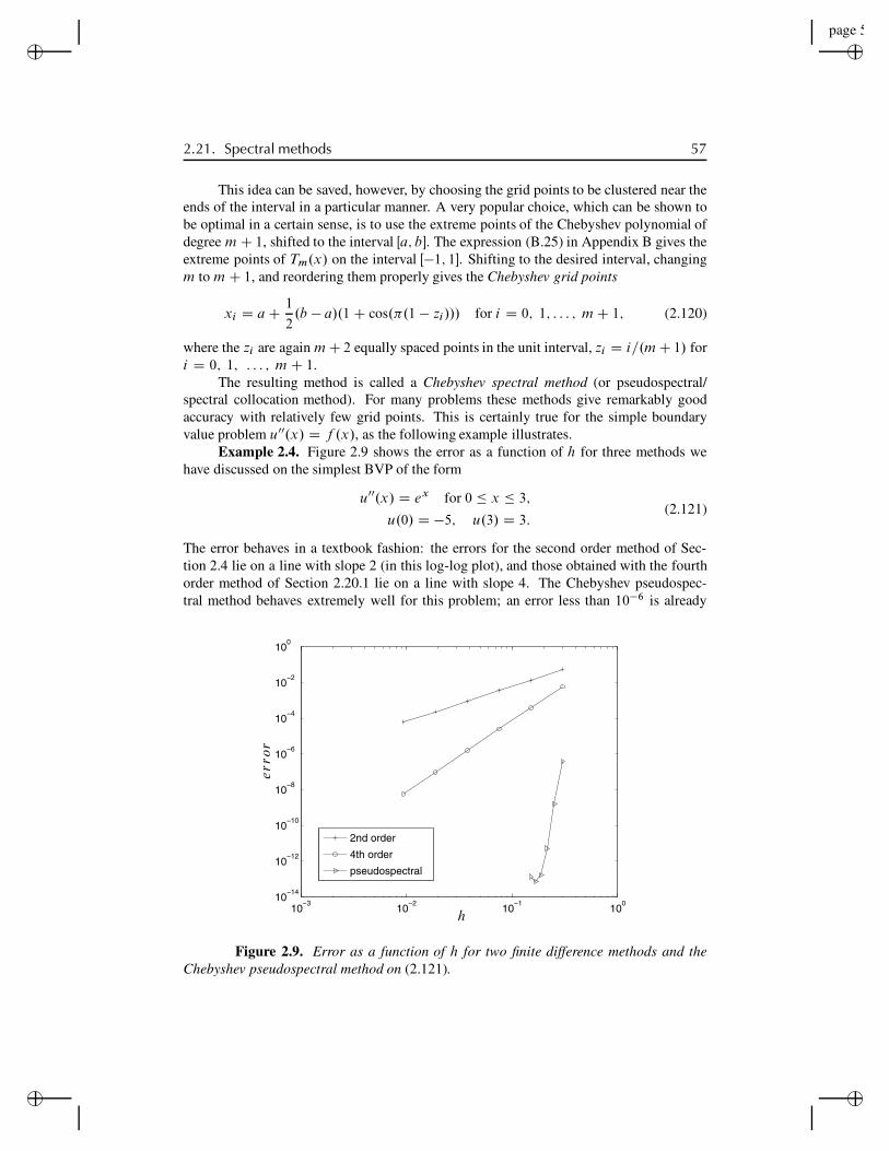
“rjlfdm”2007/6/1page 57✐
✐✐
✐
✐✐
✐✐
2.21. Spectral methods 57
This idea can be saved, however, by choosing the grid points to be clustered near theends of the interval in a particular manner. A very popular choice, which can be shown tobe optimal in a certain sense, is to use the extreme points of the Chebyshev polynomial ofdegree m C 1, shifted to the interval Œa; b!. The expression (B.25) in Appendix B gives theextreme points of Tm.x/ on the interval Œ!1; 1!. Shifting to the desired interval, changingm to m C 1, and reordering them properly gives the Chebyshev grid points
xi D a C 1
2.b ! a/.1 C cos.".1 ! zi/// for i D 0; 1; : : : ; m C 1; (2.120)
where the zi are again m C 2 equally spaced points in the unit interval, zi D i=.m C 1/ fori D 0; 1; : : : ; m C 1.
The resulting method is called a Chebyshev spectral method (or pseudospectral/spectral collocation method). For many problems these methods give remarkably goodaccuracy with relatively few grid points. This is certainly true for the simple boundaryvalue problem u00.x/ D f .x/, as the following example illustrates.
Example 2.4. Figure 2.9 shows the error as a function of h for three methods wehave discussed on the simplest BVP of the form
u00.x/ D ex for 0 " x " 3;
u.0/ D !5; u.3/ D 3:(2.121)
The error behaves in a textbook fashion: the errors for the second order method of Sec-tion 2.4 lie on a line with slope 2 (in this log-log plot), and those obtained with the fourthorder method of Section 2.20.1 lie on a line with slope 4. The Chebyshev pseudospec-tral method behaves extremely well for this problem; an error less than 10!6 is already
10−3
10−2
10−1
100
10−14
10−12
10−10
10−8
10−6
10−4
10−2
100
2nd order
4th order
pseudospectral
h
error
Figure 2.9. Error as a function of h for two finite difference methods and theChebyshev pseudospectral method on (2.121).

“rjlfdm”2007/6/1page 58✐
✐✐
✐
✐✐
✐✐
58 Chapter 2. Steady States and Boundary Value Problems
observed on the coarsest grid (with m D 10) and rounding errors become a problem bym D 20. The finest grids used for the finite difference methods in this figure had m D 320points.
For many problems, spectral or pseudospectral methods are well suited and should beseriously considered, although they can have difficulties of their own on realistic nonlinearproblems in complicated geometries, or for problems where the solution is not sufficientlysmooth. In fact the solution is required to be analytic in some region of the complex planesurrounding the interval over which the solution is being computed in order to get full“spectral accuracy.”
Note that the polynomial p.x/ in (2.119) is exactly the function U.x/ from (2.118),although in the way we have presented the method we do not explicitly compute the coef-ficients of this polynomial in terms of polynomial basis functions. One could compute thisinterpolating polynomial if desired once the grid values Uj are known. This may be usefulif one needs to approximate the solution u.x/ at many more points in the interval than wereused in solving the BVP.
For some problems it is natural to use Fourier series representations for the functionU.x/ in (2.118) rather than polynomials, in particular for problems with periodic boundaryconditions. In this case the dense matrix systems that arise can generally be solved usingfast Fourier transform (FFT) algorithms. The FFT also can be used in solving problemswith Chebyshev polynomials because of the close relation between these polynomials andtrigonometric functions, as discussed briefly in Section B.3.2. In many applications, how-ever, a spectral method uses sufficiently few grid points that using direct solvers (Gaussianelimination) is a reasonable approach.
The analysis and proper application of pseudospectral methods goes well beyond thescope of this book. See, for example, [10], [14], [29], [38], or [90] for more thoroughintroductions to spectral methods.
Note also that spectral approximation of derivatives often is applied only in spatialdimensions. For time-dependent problems, a time-stepping procedure is often based onfinite difference methods, of the sort developed in Part II of this book. For PDEs this timestepping may be coupled with a spectral approximation of the spatial derivatives, a topic webriefly touch on in Sections 9.9 and 10.13. One time-stepping procedure that has the flavorof a spectral procedure in time is the recent spectral deferred correction method presentedin [28].
“rjlfdm”2007/6/1page 59✐
✐✐
✐
✐✐
✐✐
Chapter 3
Elliptic Equations
In more than one space dimension, the steady-state equations discussed in Chapter 2 gen-eralize naturally to elliptic partial differential equations, as discussed in Section E.1.2. Intwo space dimensions a constant-coefficient elliptic equation has the form
a1uxx C a2uxy C a3uyy C a4ux C a5uy C a6u D f; (3.1)
where the coefficients a1; a2; a3 satisfy
a22 ! 4a1a3 < 0: (3.2)
This equation must be satisfied for all .x; y/ in some region of the plane !, together withsome boundary conditions on @!, the boundary of !. For example, we may have Dirichletboundary conditions in which case u.x; y/ is given at all points .x; y/ 2 @!. If the ellip-ticity condition (3.2) is satisfied, then this gives a well-posed problem. If the coefficientsvary with x and y, then the ellipticity condition must be satisfied at each point in !.
3.1 Steady-state heat conductionEquations of elliptic character often arise as steady-state equations in some region of space,associated with some time-dependent physical problem. For example, the diffusion or heatconduction equation in two space dimensions takes the form
ut D ."ux /x C ."uy/y C ; (3.3)
where ".x; y/ > 0 is a diffusion or heat conduction coefficient that may vary with x andy, and .x; y; t/ is a source term. The solution u.x; y; t/ generally will vary with timeas well as space. We also need initial conditions u.x; y; 0/ in ! and boundary conditionsat each point in time at every point on the boundary of !. If the boundary conditions andsource terms are independent of time, then we expect a steady state to exist, which we canfind by solving the elliptic equation
."ux /x C ."uy /y D f; (3.4)
59
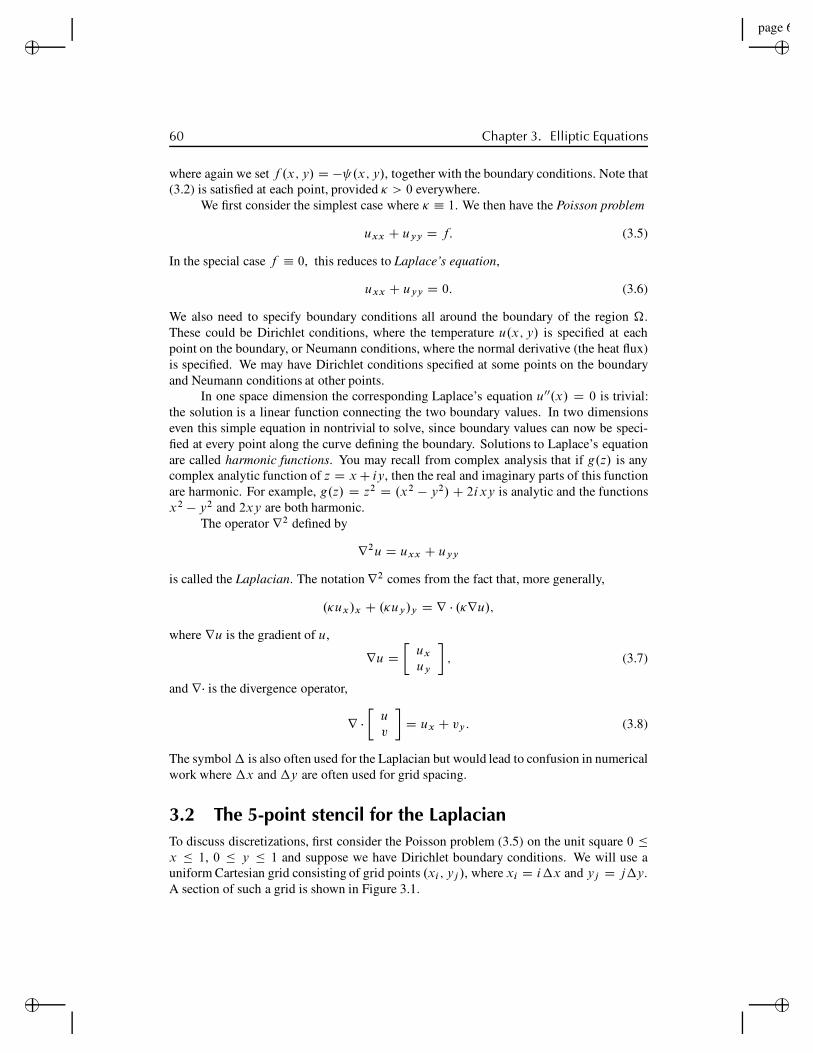
“rjlfdm”2007/6/1page 60✐
✐✐
✐
✐✐
✐✐
60 Chapter 3. Elliptic Equations
where again we set f .x; y/ D ! .x; y/, together with the boundary conditions. Note that(3.2) is satisfied at each point, provided ! > 0 everywhere.
We first consider the simplest case where ! " 1. We then have the Poisson problem
uxx C uyy D f: (3.5)
In the special case f " 0, this reduces to Laplace’s equation,
uxx C uyy D 0: (3.6)
We also need to specify boundary conditions all around the boundary of the region ".These could be Dirichlet conditions, where the temperature u.x; y/ is specified at eachpoint on the boundary, or Neumann conditions, where the normal derivative (the heat flux)is specified. We may have Dirichlet conditions specified at some points on the boundaryand Neumann conditions at other points.
In one space dimension the corresponding Laplace’s equation u00.x/ D 0 is trivial:the solution is a linear function connecting the two boundary values. In two dimensionseven this simple equation in nontrivial to solve, since boundary values can now be speci-fied at every point along the curve defining the boundary. Solutions to Laplace’s equationare called harmonic functions. You may recall from complex analysis that if g.z/ is anycomplex analytic function of z D x C iy, then the real and imaginary parts of this functionare harmonic. For example, g.z/ D z2 D .x2 ! y2/ C 2ixy is analytic and the functionsx2 ! y2 and 2xy are both harmonic.
The operator r2 defined by
r2u D uxx C uyy
is called the Laplacian. The notation r2 comes from the fact that, more generally,
.!ux/x C .!uy/y D r # .!ru/;
where ru is the gradient of u,
ru D!
ux
uy
"; (3.7)
and r# is the divergence operator,
r #!
uv
"D ux C vy : (3.8)
The symbol # is also often used for the Laplacian but would lead to confusion in numericalwork where #x and #y are often used for grid spacing.
3.2 The 5-point stencil for the LaplacianTo discuss discretizations, first consider the Poisson problem (3.5) on the unit square 0 $x $ 1, 0 $ y $ 1 and suppose we have Dirichlet boundary conditions. We will use auniform Cartesian grid consisting of grid points .xi ; yj /, where xi D i#x and yj D j#y.A section of such a grid is shown in Figure 3.1.
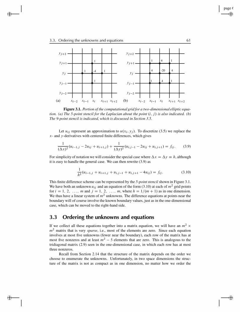
“rjlfdm”2007/6/1page 61✐
✐✐
✐
✐✐
✐✐
3.3. Ordering the unknowns and equations 61
(a)
1
1
-4 1
1
xixi!1 xiC1xi!2 xiC2
yj
yj!1
yjC1
yj!2
yjC2
(b)
-204 4
4
4 1
11
1
xixi!1 xiC1xi!2 xiC2
yj
yj!1
yjC1
yj!2
yjC2
Figure 3.1. Portion of the computationalgrid for a two-dimensionalelliptic equa-tion. (a) The 5-point stencil for the Laplacian about the point .i; j / is also indicated. (b)The 9-point stencil is indicated, which is discussed in Section 3.5.
Let uij represent an approximation to u.xi ; yj /. To discretize (3.5) we replace thex- and y-derivatives with centered finite differences, which gives
1
.!x/2.ui!1;j ! 2uij C uiC1;j /C 1
.!y/2.ui;j!1 ! 2uij C ui;jC1/ D fij : (3.9)
For simplicity of notation we will consider the special case where !x D !y " h, althoughit is easy to handle the general case. We can then rewrite (3.9) as
1
h2.ui!1;j C uiC1;j C ui;j!1 C ui;jC1 ! 4uij / D fij : (3.10)
This finite difference scheme can be represented by the 5-point stencil shown in Figure 3.1.We have both an unknown uij and an equation of the form (3.10) at each of m2 grid pointsfor i D 1; 2; : : : ; m and j D 1; 2; : : : ; m, where h D 1=.m C 1/ as in one dimension.We thus have a linear system of m2 unknowns. The difference equations at points near theboundary will of course involve the known boundary values, just as in the one-dimensionalcase, which can be moved to the right-hand side.
3.3 Ordering the unknowns and equationsIf we collect all these equations together into a matrix equation, we will have an m2 #m2 matrix that is very sparse, i.e., most of the elements are zero. Since each equationinvolves at most five unknowns (fewer near the boundary), each row of the matrix has atmost five nonzeros and at least m2 ! 5 elements that are zero. This is analogous to thetridiagonal matrix (2.9) seen in the one-dimensional case, in which each row has at mostthree nonzeros.
Recall from Section 2.14 that the structure of the matrix depends on the order wechoose to enumerate the unknowns. Unfortunately, in two space dimensions the struc-ture of the matrix is not as compact as in one dimension, no matter how we order the
“rjlfdm”2007/6/1page 62✐
✐✐
✐
✐✐
✐✐
62 Chapter 3. Elliptic Equations
unknowns, and the nonzeros cannot be as nicely clustered near the main diagonal. Oneobvious choice is the natural rowwise ordering, where we take the unknowns along thebottom row, u11; u21; u31; : : : ; um1, followed by the unknowns in the second row,u12; u22; : : : ;um2, and so on, as illustrated in Figure 3.2(a). The vector of unknownsis partitioned as
u D
2
6664
uŒ1!
uŒ2!
:::
uŒm!
3
7775 ; where uŒj ! D
2
6664
u1j
u2j
:::umj
3
7775 : (3.11)
This gives a matrix equation where A has the form
A D 1
h2
2
666664
T II T I
I T I: : :
: : :: : :
I T
3
777775; (3.12)
which is an m !m block tridiagonal matrix in which each block T or I is itself an m ! mmatrix,
T D
2
666664
"4 11 "4 1
1 "4 1: : :
: : :: : :
1 "4
3
777775;
and I is the m ! m identity matrix. While this has a nice structure, the 1 values in the Imatrices are separated from the diagonal by m"1 zeros, since these coefficients correspondto grid points lying above or below the central point in the stencil and hence are in the nextor previous row of unknowns.
Another possibility, which has some advantages in the context of certain iterativemethods, is to use the red-black ordering (or checkerboard ordering) shown in Figure 3.2.This is the two-dimensional analogue of the odd-even ordering that leads to the matrix(2.63) in one dimension. This ordering is significant because all four neighbors of a red gridpoint are black points, and vice versa, and it leads to a matrix equation with the structure
!D H
H T D
" !ured
ublack
"D!
fred
"fblack
"; (3.13)
where D D " 4h2 I is a diagonal matrix of dimension m2=2 and H is a banded matrix of
the same dimension with four nonzero diagonals.When direct methods such as Gaussian elimination are used to solve the system, one
typically wants to order the equations and unknowns so as to reduce the amount of fill-induring the elimination procedure as much as possible. This is done automatically if thebackslash operator in MATLAB is used to solve the system, provided it is set up usingsparse storage; see Section 3.7.1.

“rjlfdm”2007/6/1page 63✐
✐✐
✐
✐✐
✐✐
3.4. Accuracy and stability 63
(a)
41 2 3
5 6 7 8
9 10 11 12
13 14 15 16
(b)
15
9 2
13 14
10
65
1
11 3 12 4
16 87
Figure 3.2. (a) The natural rowwise order of unknowns and equations on a 4 ! 4grid. (b) The red-black ordering.
3.4 Accuracy and stabilityThe discretization of the two-dimensional Poisson problem can be analyzed using exactlythe same approach as we used for the one-dimensional boundary value problem. The localtruncation error !ij at the .i; j / grid point is defined in the obvious way,
!ij D 1
h2.u.xi!1; yj /Cu.xiC1; yj /Cu.xi ; yj!1/Cu.xi ; yjC1/"4u.xi ; yj //"f .xi ; yj /;
and by splitting this into the second order difference in the x- and y-directions it is clearfrom previous results that
!ij D 1
12h2.uxxxx C uyyyy/C O.h4/:
For this linear system of equations the global error Eij D uij " u.xi ; yj / then solves thelinear system
AhEh D "!h
just as in one dimension, where Ah is now the discretization matrix with mesh spacing h,e.g., the matrix (3.12) if the rowwise ordering is used. The method will be globally secondorder accurate in some norm provided that it is stable, i.e., that k.Ah/!1k is uniformlybounded as h ! 0.
In the 2-norm this is again easy to check for this simple problem, since we can explic-itly compute the spectral radius of the matrix, as we did in one dimension in Section 2.10.The eigenvalues and eigenvectors of A can now be indexed by two parameters p and kcorresponding to wave numbers in the x- and y-directions for p; k D 1; 2; : : : ; m. The.p; q/ eigenvector up;q has the m2 elements
up;qij D sin.p" ih/ sin.q"j h/: (3.14)
The corresponding eigenvalue is
#p;q D 2
h2..cos.p"h/ " 1/C .cos.q"h/ " 1// : (3.15)
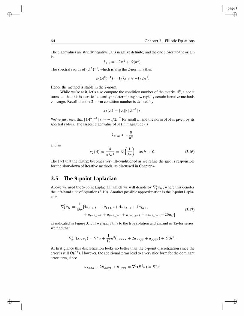
“rjlfdm”2007/6/1page 64✐
✐✐
✐
✐✐
✐✐
64 Chapter 3. Elliptic Equations
The eigenvalues are strictly negative (A is negative definite) and the one closest to the originis
!1;1 D !2"2 C O.h2/:
The spectral radius of .Ah/!1, which is also the 2-norm, is thus
#..Ah/!1/ D 1=!1;1 " !1=2"2:
Hence the method is stable in the 2-norm.While we’re at it, let’s also compute the condition number of the matrix Ah, since it
turns out that this is a critical quantity in determining how rapidly certain iterative methodsconverge. Recall that the 2-norm condition number is defined by
$2.A/ D kAk2kA!1k2:
We’ve just seen that k.Ah/!1k2 " !1=2"2 for small h, and the norm of A is given by itsspectral radius. The largest eigenvalue of A (in magnitude) is
!m;m " ! 8
h2
and so
$2.A/ "4
"2h2D O
!1
h2
"as h ! 0: (3.16)
The fact that the matrix becomes very ill-conditioned as we refine the grid is responsiblefor the slow-down of iterative methods, as discussed in Chapter 4.
3.5 The 9-point LaplacianAbove we used the 5-point Laplacian, which we will denote by r2
5 uij , where this denotesthe left-hand side of equation (3.10). Another possible approximation is the 9-point Lapla-cian
r29 uij D 1
6h2Œ4ui!1;j C 4uiC1;j C 4ui;j!1 C 4ui;jC1
C ui!1;j!1 C ui!1;jC1 C uiC1;j!1 C uiC1;jC1 ! 20uij %(3.17)
as indicated in Figure 3.1. If we apply this to the true solution and expand in Taylor series,we find that
r29 u.xi; yj / D r2u C 1
12h2.uxxxx C 2uxxyy C uyyyy/C O.h4/:
At first glance this discretization looks no better than the 5-point discretization since theerror is still O.h2/. However, the additional terms lead to a very nice form for the dominanterror term, since
uxxxx C 2uxxyy C uyyyy D r2.r2u/ # r4u:
“rjlfdm”2007/6/1page 65✐
✐✐
✐
✐✐
✐✐
3.5. The 9-point Laplacian 65
This is the Laplacian of the Laplacian of u and r4 is called the biharmonic operator. If weare solving r2u D f , then we have
uxxxx C 2uxxyy C uyyyy D r2f:
Hence we can compute the dominant term in the truncation error easily from the knownfunction f without knowing the true solution u to the problem.
In particular, if we are solving Laplace’s equation, where f D 0, or more gener-ally if f is a harmonic function, then this term in the local truncation error vanishes andthe 9-point Laplacian would give a fourth order accurate discretization of the differentialequation.
More generally, we can obtain a fourth order accurate method of the form
r29 uij D fij (3.18)
for arbitrary smooth functions f .x; y/ by defining
fij D f .xi ; yj /C h2
12r2f .xi ; yj /: (3.19)
We can view this as deliberately introducing an O.h2/ error into the right-hand side of theequation that is chosen to cancel the O.h2/ part of the local truncation error. Taylor seriesexpansion easily shows that the local truncation error of the method (3.18) is now O.h4/.This is the two-dimensional analogue of the modification (2.117) that gives fourth orderaccuracy for the boundary value problem u00.x/ D f .x/.
If we have only data f .xi ; yj / at the grid points (but we know that the underlyingfunction is sufficiently smooth), then we can still achieve fourth order accuracy by using
fij D f .xi ; yj /C h2
12r2
5f .xi ; yj /
instead of (3.19).This is a trick that often can be used in developing numerical methods—introducing
an “error” into the equations that is carefully chosen to cancel some other error.Note that the same trick wouldn’t work with the 5-point Laplacian, or at least not as
directly. The form of the truncation error in this method depends on uxxxx C uyyyy. Thereis no way to compute this directly from the original equation without knowing u. The extrapoints in the 9-point stencil convert this into the Laplacian of f , which can be computed iff is sufficiently smooth.
On the other hand, a two-pass approach could be used with the 5-point stencil, inwhich we first estimate u by solving with the standard 5-point scheme to get a second orderaccurate estimate of u. We then use this estimate of u to approximate uxxxx C uyyyy andthen solve a second time with a right-hand side that is modified to eliminate the dominantterm of the local truncation error. This would be more complicated for this particularproblem, but this idea can be used much more generally than the above trick, which dependson the special form of the Laplacian. This is the method of deferred corrections, alreadydiscussed for one dimension in Section 2.20.3.
“rjlfdm”2007/6/1page 66✐
✐✐
✐
✐✐
✐✐
66 Chapter 3. Elliptic Equations
3.6 Other elliptic equationsIn Chapter 2 we started with the simplest boundary value problem for the constant coeffi-cient problem u00.x/ D f .x/ but then introduced various, more interesting problems, suchas variable coefficients, nonlinear problems, singular perturbation problems, and boundaryor interior layers.
In the multidimensional case we have discussed only the simplest Poisson problem,which in one dimension reduces to u00.x/ D f .x/. All the further complications seen inone dimension can also arise in multidimensional problems. For example, heat conductionin a heterogeneous two-dimensional domain gives rise to the equation
.!.x; y/ux .x; y//x C .!.x; y/uy .x; y//y D f .x; y/; (3.20)
where !.x; y/ is the varying heat conduction coefficient. In any number of space dimen-sions this equation can be written as
r ! .!ru/ D f: (3.21)
These problems can be solved by generalizations of the one-dimensional methods. Theterms .!.x; y/ux .x; y//x and .!.x; y/uy .x; y//y can each be discretized as in the one-dimensional case, again resulting in a 5-point stencil in two dimensions.
Nonlinear elliptic equations also arise in multidimensions, in which case a system ofnonlinear algebraic equations will result from the discretization. A Newton method can beused as in one dimension, but now in each Newton iteration a large sparse linear system willhave to be solved. Typically the Jacobian matrix has a sparsity pattern similar to those seenabove for linear elliptic equations. See Section 4.5 for a brief discussion of Newton–Kryloviterative methods for such problems.
In multidimensional problems there is an additional potential complication that isnot seen in one dimension: the domain " where the boundary value problem is posedmay not be a simple rectangle as we have supposed in our discussion so far. When thesolution exhibits boundary or interior layers, then we would also like to cluster grid pointsor adaptively refine the grid in these regions. This often presents a significant challengethat we will not tackle in this book.
3.7 Solving the linear systemTwo fundamentally different approaches could be used for solving the large linear systemsthat arise from discretizing elliptic equations. A direct method such as Gaussian eliminationproduces an exact solution (or at least would in exact arithmetic) in a finite number ofoperations. An iterative method starts with an initial guess for the solution and attempts toimprove it through some iterative procedure, halting after a sufficiently good approximationhas been obtained.
For problems with large sparse matrices, iterative methods are often the method ofchoice, and Chapter 4 is devoted to a study of several iterative methods. Here we brieflyconsider the operation counts for Gaussian elimination to see the potential pitfalls of thisapproach.
It should be noted, however, that on current computers direct methods can be suc-cessfully used for quite large problems, provided appropriate sparse storage and efficient
“rjlfdm”2007/6/1page 67✐
✐✐
✐
✐✐
✐✐
3.7. Solving the linear system 67
elimination procedures are used. See Section 3.7.1 for some comments on setting up sparsematrices such as (3.12) in MATLAB.
It is well known (see, e.g., [35], [82], [91]) that for a general N ! N dense matrix(one with few elements equal to zero), performing Gaussian elimination requires O.N 3/operations. (There are N .N " 1/=2 D O.N 2/ elements below the diagonal to eliminate,and eliminating each one requires O.N / operations to take a linear combination of therows.)
Applying a general Gaussian elimination program blindly to the matrices we arenow dealing with would be disastrous, or at best extremely wasteful of computer resources.Suppose we are solving the three-dimensional Poisson problem on a 100!100!100 grid—a modest problem these days. Then N D m3 D 106 and N 3 D 1018. On a reasonably fastdesktop that can do on the order of 1010 floating point operations per second (10 gigaflops),this would take on the order of 108 seconds, which is more than 3 years. More sophisticatedmethods can solve this problem in seconds.
Moreover, even if speed were not an issue, memory would be. Storing the full matrixA in order to modify the elements and produce L and U would require N 2 memory loca-tions. In 8-byte arithmetic this requires 8 N 2 bytes. For the problem mentioned above, thiswould be 8!1012 bytes, or eight terabytes. One advantage of iterative methods is that theydo not store the matrix at all and at most need to store the nonzero elements.
Of course with Gaussian elimination it would be foolish to store all the elements ofa sparse matrix, since the vast majority are zero, or to apply the procedure blindly withouttaking advantage of the fact that so many elements are already zero and hence do not needto be eliminated.
As an extreme example, consider the one-dimensional case where we have a tridi-agonal matrix as in (2.9). Applying Gaussian elimination requires eliminating only thenonzeros along the subdiagonal, only N " 1 values instead of N .N " 1/=2. Moreover,when we take linear combinations of rows in the course of eliminating these values, inmost columns we will be taking linear combinations of zeros, producing zero again. If wedo not do pivoting, then only the diagonal elements are modified. Even with partial pivot-ing, at most we will introduce one extra superdiagonal of nonzeros in the upper triangularU that were not present in A. As a result, it is easy to see that applying Gaussian elimina-tion to an m ! m tridiagonal system requires only O.m/ operations, not O.m3/, and thatthe storage required is O.m/ rather than O.m2/.
Note that this is the best we could hope for in one dimension, at least in terms of theorder of magnitude. There are m unknowns and even if we had exact formulas for thesevalues, it would require O.m/ work to evaluate them and O.m/ storage to save them.
In two space dimensions we can also take advantage of the sparsity and structureof the matrix to greatly reduce the storage and work required with Gaussian elimination,although not to the minimum that one might hope to attain. On an m ! m grid there areN D m2 unknowns, so the best one could hope for is an algorithm that computes thesolution in O.N / D O.m2/ work using O.m2/ storage. Unfortunately, this cannot beachieved with a direct method.
One approach that is better than working with the full matrix is to observe that the Ais a banded matrix with bandwidth m both above and below the diagonal. Since a generalN ! N banded matrix with a nonzero bands above the diagonal and b below the diagonal
“rjlfdm”2007/6/1page 68✐
✐✐
✐
✐✐
✐✐
68 Chapter 3. Elliptic Equations
can be factored in O.Nab/ operations, this results in an operation count of O.m4/ for thetwo-dimensional Poisson problem.
A more sophisticated approach that takes more advantage of the special structure (andthe fact that there are already many zeros within the bandwidth) is the nested dissectionalgorithm [34]. This algorithm requires O.m3/ operations in two dimensions. It turns outthis is the best that can be achieved with a direct method based on Gaussian elimination.George proved (see [34]) that any elimination method for solving this problem requires atleast O.m3/ operations.
For certain special problems, very fast direct methods can be used, which are muchbetter than standard Gaussian elimination. In particular, for the Poisson problem on arectangular domain there are fast Poisson solvers based on the fast Fourier transform thatcan solve on an m!m grid in two dimensions in O.m2 log m/ operations, which is nearlyoptimal. See [87] for a review of this approach.
3.7.1 Sparse storage in MATLABIf you are going to work in MATLAB with sparse matrices arising from finite differencemethods, it is important to understand and use the sparse matrix commands that set upmatrices using sparse storage, so that only the nonzeros are stored. Type help sparseto get started.
As one example, the matrix of (3.12) can be formed in MATLAB by the commands
I = eye(m);e = ones(m,1);T = spdiags([e -4*e e],[-1 0 1],m,m);S = spdiags([e e],[-1 1],m,m);A = (kron(I,T) + kron(S,I))/hˆ2;
The spy(A) command is also useful for looking at the nonzero structure of a matrix.The backslash command in MATLAB can be used to solve systems using sparse
storage, and it implements highly efficient direct methods using sophisticated algorithmsfor dynamically ordering the equations to minimize fill-in, as described by Davis [24].

“rjlfdm”2007/6/1page 69✐
✐✐
✐
✐✐
✐✐
Chapter 4
Iterative Methods forSparse Linear Systems
This chapter contains an overview of several iterative methods for solving the large sparselinear systems that arise from discretizing elliptic equations. Large sparse linear systemsarise from many other practical problems, too, of course, and the methods discussed hereare useful in other contexts as well. Except when the matrix has very special structure andfast direct methods of the type discussed in Section 3.7 apply, iterative methods are usuallythe method of choice for large sparse linear systems.
The classical Jacobi, Gauss–Seidel, and successive overrelaxation (SOR) methodsare introduced and briefly discussed. The bulk of the chapter, however, concerns moremodern methods for solving linear systems that are typically much more effective for large-scale problems: preconditioned conjugate-gradient (CG) methods, Krylov space methodssuch as generalized minimum residual (GMRES), and multigrid methods.
4.1 Jacobi and Gauss–SeidelIn this section two classical iterative methods, Jacobi and Gauss–Seidel, are introduced toillustrate the main issues. It should be stressed at the beginning that these are poor methodsin general which converge very slowly when used as standalone methods, but they havethe virtue of being simple to explain. Moreover, these methods are sometimes used asbuilding blocks in more sophisticated methods, e.g., Jacobi may be used as a smoother forthe multigrid method, as discussed in Section 4.6.
We again consider the Poisson problem where we have the system of equations(3.10). We can rewrite this equation as
uij D 1
4.ui!1;j C uiC1;j C ui;j!1 C ui;jC1/ !
h2
4fij : (4.1)
In particular, note that for Laplace’s equation (where fij " 0), this simply states that thevalue of u at each grid point should be the average of its four neighbors. This is the discreteanalogue of the well-known fact that a harmonic function has the following property: thevalue at any point .x; y/ is equal to the average value around a closed curve containing thepoint, in the limit as the curve shrinks to the point. Physically this also makes sense if we
69
“rjlfdm”2007/6/1page 70✐
✐✐
✐
✐✐
✐✐
70 Chapter 4. Iterative Methods for Sparse Linear Systems
think of the heat equation. Unless the temperature at this point is equal to the average ofthe temperature at neighboring points, there will be a net flow of heat toward or away fromthis point.
The equation (4.1) suggests the following iterative method to produce a new estimateuŒkC1! from a current guess uŒk!:
uŒkC1!ij D 1
4
!u
Œk!i!1;j C u
Œk!iC1;j C u
Œk!i;j!1 C u
Œk!i;jC1
"! h2
4fij : (4.2)
This is the Jacobi iteration for the Poisson problem, and it can be shown that for thisparticular problem it converges from any initial guess uŒ0! (although very slowly).
Here is a short section of MATLAB code that implements the main part of this itera-tion:
for iter=0:maxiterfor j=2:(m+1)
for i=2:(m+1)unew(i,j) = 0.25*(u(i-1,j) + u(i+1,j) + ...
u(i,j-1) + u(i,j+1) - hˆ2 * f(i,j));end
endu = unew;end
Here it is assumed that u initially contains the guess uŒ0! and that boundary data are storedin u(1,:), u(m+2,:), u(:,1), and u(:,m+2). The indexing is off by 1 fromwhat might be expected since MATLAB begins arrays with index 1, not 0.
Note that one might be tempted to dispense with the variable unew and replace theabove code with
for iter=0:maxiterfor j=2:(m+1)
for i=2:(m+1)u(i,j) = 0.25*(u(i-1,j) + u(i+1,j) + ...
u(i,j-1) + u(i,j+1) - hˆ2 * f(i,j));end
endend
This would not give the same results, however. In the correct code for Jacobi wecompute new values of u based entirely on old data from the previous iteration, as requiredfrom (4.2). In the second code we have already updated u(i-1,j) and u(i,j-1)before updating u(i,j), and these new values will be used instead of the old ones. Thelatter code thus corresponds to the method
uŒkC1!ij D 1
4
!uŒkC1!
i!1;j C uŒk!iC1;j C uŒkC1!
i;j!1 C uŒk!i;jC1
"! h2
4fij : (4.3)
This is what is known as the Gauss–Seidel method, and it would be a lucky coding er-ror since this method generally converges about twice as fast as Jacobi does. The Jacobi
“rjlfdm”2007/6/1page 71✐
✐✐
✐
✐✐
✐✐
4.2. Analysis of matrix splitting methods 71
method is sometimes called the method of simultaneous displacements, while Gauss–Seidelis known as the method of successive displacements. Later we’ll see that Gauss–Seidel canbe improved by using SOR.
Note that if one actually wants to implement Jacobi in MATLAB, looping over i andj is quite slow and it is much better to write the code in vectorized form, e.g.,
I = 2:(m+1);J = 2:(m+1);for iter=0:maxiter
u(I,J) = 0.25*(u(I-1,J) + u(I+1,J) + u(I,J-1) ...+ u(I,J+1) - hˆ2 * f(I,J));
end
It is somewhat harder to implement Gauss–Seidel in vectorized form.Convergence of these methods will be discussed in Section 4.2. First we note some
important features of these iterative methods:
! The matrix A is never stored. In fact, for this simple constant coefficient problem, wedon’t even store all the 5m2 nonzeros which all have the value 1=h2 or "4=h2. Thevalues 0:25 and h2 in the code are the only values that are “stored.” (For a variablecoefficient problem where the coefficients are different at each point, we would ingeneral have to store all the nonzeros.)
! Hence the storage is optimal—essentially only the m2 solution values are stored inthe Gauss–Seidel method. The above code for Jacobi uses 2m2 since unew is storedas well as u, but one could eliminate most of this with more careful coding.
! Each iteration requires O.m2/ work. The total work required will depend on howmany iterations are required to reach the desired level of accuracy. We will see thatwith these particular methods we require O.m2 log m/ iterations to reach a level ofaccuracy consistent with the expected global error in the solution (as h ! 0 weshould require more accuracy in the solution to the linear system). Combining thiswith the work per iteration gives a total operation count of O.m4 log m/. This looksworse than Gaussian elimination with a banded solver, although since log m growsso slowly with m it is not clear which is really more expensive for a realistic-sizematrix. (And the iterative method definitely saves on storage.)
Other iterative methods also typically require O.m2/ work per iteration but mayconverge much faster and hence result in less overall work. The ideal would be to convergein a number of iterations that is independent of h so that the total work is simply O.m2/.Multigrid methods (see Section 4.6) can achieve this, not only for Poisson’s problem butalso for many other elliptic equations.
4.2 Analysis of matrix splitting methodsIn this section we study the convergence of the Jacobi and Gauss–Seidel methods. As asimple example we will consider the one-dimensional analogue of the Poisson problem,u00.x/ D f .x/ as discussed in Chapter 2. Then we have a tridiagonal system of equations

“rjlfdm”2007/6/1page 72✐
✐✐
✐
✐✐
✐✐
72 Chapter 4. Iterative Methods for Sparse Linear Systems
(2.9) to solve. In practice we would never use an iterative method for this system, sinceit can be solved directly by Gaussian elimination in O.m/ operations, but it is easier toillustrate the iterative methods in the one-dimensional case, and all the analysis done herecarries over almost unchanged to the two-dimensional and three-dimensional cases.
The Jacobi and Gauss–Seidel methods for this problem take the form
Jacobi uŒkC1!i D 1
2
!u
Œk!i!1 C u
Œk!iC1 ! h2fi
"; (4.4)
Gauss–Seidel uŒkC1!i D 1
2
!u
ŒkC1!i!1 C u
Œk!iC1 ! h2fi
": (4.5)
Both methods can be analyzed by viewing them as based on a splitting of the matrix A into
A D M ! N; (4.6)
where M and N are two m " m matrices. Then the system Au D f can be written as
M u ! N u D f H) M u D N u C f;
which suggests the iterative method
M uŒkC1! D N uŒk! C f: (4.7)
In each iteration we assume uŒk! is known and we obtain uŒkC1! by solving a linear systemwith the matrix M . The basic idea is to define the splitting so that M contains as muchof A as possible (in some sense) while keeping its structure sufficiently simple that thesystem (4.7) is much easier to solve than the original system with the full A. Since systemsinvolving diagonal, lower, or upper triangular matrices are relatively simple to solve, thereare some obvious choices for the matrix M . To discuss these in a unified framework, write
A D D ! L! U (4.8)
in general, where D is the diagonal of A, !L is the strictly lower triangular part, and !Uis the strictly upper triangular part. For example, the tridiagonal matrix (2.10) would give
D D 1
h2
2
66666664
!2 00 !2 0
0 !2 0: : :
: : :: : :
0 !2 00 !2
3
77777775
; L D ! 1
h2
2
66666664
0 01 0 0
1 0 0: : :
: : :: : :
1 0 01 0
3
77777775
with !U D !LT being the remainder of A.In the Jacobi method, we simply take M to be the diagonal part of A, M D D, so
that
M D ! 2
h2I; N D L C U D D ! A D ! 1
h2
2
66666664
0 11 0 1
1 0 1: : :
: : :: : :
1 0 11 0
3
77777775
:
“rjlfdm”2007/6/1page 73✐
✐✐
✐
✐✐
✐✐
4.2. Analysis of matrix splitting methods 73
The system (4.7) is then diagonal and extremely easy to solve:
uŒkC1! D 1
2
2
66666664
0 11 0 1
1 0 1: : :
: : :: : :
1 0 11 0
3
77777775
uŒk! ! h2
2f; (4.9)
which agrees with (4.4).In Gauss–Seidel, we take M to be the full lower triangular portion of A, so M D
D ! L and N D U . The system (4.7) is then solved using forward substitution, whichresults in (4.5).
To analyze these methods, we derive from (4.7) the update formula
uŒkC1! D M !1N uŒk! C M !1f
" GuŒk! C c;(4.10)
where G D M !1N is the iteration matrix and c D M !1f .Let u" represent the true solution to the system Au D f . Then
u" D Gu" C c: (4.11)
This shows that the true solution is a fixed point, or equilibrium, of the iteration (4.10),i.e., if uŒk! D u", then uŒkC1! D u" as well. However, it is not clear that this is a stableequilibrium, i.e., that we would converge toward u" if we start from some incorrect initialguess.
If eŒk! D uŒk! ! u" represents the error, then subtracting (4.11) from (4.10) gives
eŒkC1! D GeŒk!;
and so after k steps we haveeŒk! D Gk eŒ0!: (4.12)
From this we can see that the method will converge from any initial guess uŒ0!, providedGk ! 0 (an m # m matrix of zeros) as k ! 1. When is this true?
For simplicity, assume that G is a diagonalizable matrix, so that we can write
G D R!R!1;
where R is the matrix of right eigenvectors of G and ! is a diagonal matrix of eigenvalues"1; "2; : : : ; "m. Then
Gk D R!k R!1; (4.13)
where
!k D
2
6664
" k1
" k2
: : :
" km
3
7775:
“rjlfdm”2007/6/1page 74✐
✐✐
✐
✐✐
✐✐
74 Chapter 4. Iterative Methods for Sparse Linear Systems
Clearly the method converges if j!pj < 1 for all p D 1; 2; : : : ; m, i.e., if ".G/ < 1, where" is the spectral radius. See Appendix D for a more general discussion of the asymptoticproperties of matrix powers.
4.2.1 Rate of convergenceFrom (4.12) we can also determine how rapidly the method can be expected to converge incases where it is convergent. Using (4.13) in (4.12) and using the 2-norm, we obtain
keŒk!k2 ! k#k k2kRk2kR!1k2keŒ0!k2 D "k$2.R/keŒ0!k2; (4.14)
where " " ".G/, and $2.R/ D kRk2kR!1k2 is the condition number of the eigenvectormatrix.
If the matrix G is a normal matrix (see Section C.4), then the eigenvectors are or-thogonal and $2.R/ D 1. In this case we have
keŒk!k2 ! "kkeŒ0!k2: (4.15)
If G is nonnormal, then the spectral radius of G gives information about the asymp-totic rate of convergence as k ! 1 but may not give a good indication of the behaviorof the error for small k . See Section D.4 for more discussion of powers of nonnormal ma-trices and see Chapters 24–27 of [92] for some discussion of iterative methods on highlynonnormal problems.
Note: These methods are linearly convergent, in the sense that keŒkC1!k ! "keŒk!kand it is the first power of keŒk!k that appears on the right. Recall that Newton’s method istypically quadratically convergent, and it is the square of the previous error that appears onthe right-hand side. But Newton’s method is for a nonlinear problem and requires solvinga linear system in each iteration. Here we are looking at solving such a linear system.
Example 4.1. For the Jacobi method we have
G D D!1.D # A/ D I # D!1A:
If we apply this method to the boundary value problem u00 D f , then
G D I C h2
2A:
The eigenvectors of this matrix are the same as the eigenvectors of A, and the eigenvaluesare hence
!p D 1 C h2
2%p ;
where %p is given by (2.23). So
!p D cos.p&h/; p D 1; 2; : : : ; m;
where h D 1=.m C 1/. The spectral radius is
".G/ D j!1j D cos.&h/ $ 1 # 1
2&2h2 C O.h4/: (4.16)

“rjlfdm”2007/6/1page 75✐
✐✐
✐
✐✐
✐✐
4.2. Analysis of matrix splitting methods 75
The spectral radius is less than 1 for any h > 0 and the Jacobi method converges. Moreover,the G matrix for Jacobi is symmetric as seen in (4.9), and so (4.15) holds and the error ismonotonically decreasing at a rate given precisely by the spectral radius. Unfortunately,though, for small h this value is very close to 1, resulting in very slow convergence.
How many iterations are required to obtain a good solution? Suppose we want toreduce the error to keŒk!k ! !keŒ0!k (where typically keŒ0!k is on the order of 1).1 Then wewant "k ! ! and so
k ! log.!/= log."/: (4.17)
How small should we choose !? To get full machine precision we might choose ! to beclose to the machine round-off level. However, this typically would be very wasteful. Forone thing, we rarely need this many correct digits. More important, however, we shouldkeep in mind that even the exact solution u! of the linear system Au D f is only anapproximate solution of the differential equation we are actually solving. If we are using asecond order accurate method, as in this example, then u!
i differs from u.xi/ by somethingon the order of h2 and so we cannot achieve better accuracy than this no matter how wellwe solve the linear system. In practice we should thus take ! to be something related to theexpected global error in the solution, e.g., ! D C h2 for some fixed C .
To estimate the order of work required asymptotically as h ! 0, we see that theabove choice gives
k D .log.C /C 2 log.h//= log."/: (4.18)
For Jacobi on the boundary value problem we have " ! 1 " 12#2h2 and hence log."/ !
"12#
2h2. Since h D 1=.m C 1/, using this in (4.18) gives
k D O.m2 log m/ as m ! 1: (4.19)
Since each iteration requires O.m/ work in this one-dimensional problem, the total workrequired to solve the problem is
total work D O.m3 log m/:
Of course this tridiagonal problem can be solved exactly in O.m/ work, so we would befoolish to use an iterative method at all here!
For a Poisson problem in two or three dimensions it can be verified that (4.19) stillholds, although now the work required per iteration is O.m2/ or O.m3/, respectively, ifthere are m grid points in each direction. In two dimensions we would thus find that
total work D O.m4 log m/: (4.20)
Recall from Section 3.7 that Gaussian elimination on the banded matrix requires O.m4/operations, while other direct methods can do much better, so Jacobi is still not competitive.Luckily there are much better iterative methods.
1Assuming we are using some grid function norm, as discussed in Appendix A. Note that for the 2-norm inone dimension this requires introducing a factor of
ph in the definitions of both keŒk!k and keŒ0!k, but these
factors cancel out in choosing an appropriate !.
“rjlfdm”2007/6/1page 76✐
✐✐
✐
✐✐
✐✐
76 Chapter 4. Iterative Methods for Sparse Linear Systems
For the Gauss–Seidel method applied to the Poisson problem in any number of spacedimensions, it can be shown that
!.G/ D 1 ! "2h2 C O.h4/ as h ! 0: (4.21)
This still approaches 1 as h ! 0, but it is better than (4.16) by a factor of 2, and the numberof iterations required to reach a given tolerance typically will be half the number requiredwith Jacobi. The order of magnitude figure (4.20) still holds, however, and this methodalso is not widely used.
4.2.2 Successive overrelaxationIf we look at how iterates uŒk! behave when Gauss–Seidel is applied to a typical problem,we will often see that u
ŒkC1!i is closer to u!
i than uŒk!i was, but only by a little bit. The Gauss–
Seidel update moves ui in the right direction but is far too conservative in the amount itallows ui to move. This suggests that we use the following two-stage update, illustratedagain for the problem u00 D f :
uGSi D 1
2
!u
ŒkC1!i"1 C u
Œk!iC1 ! h2fi
";
uŒkC1!i D u
Œk!i C !
!uGS
i ! uŒk!i
";
(4.22)
where ! is some scalar parameter. If ! D 1, then uŒkC1!i D uGS
i is the Gauss–Seidelupdate. If ! > 1, then we move farther than Gauss–Seidel suggests. In this case themethod is known as successive overrelaxation (SOR).
If ! < 1, then we would be underrelaxing, rather than overrelaxing. This would beeven less effective than Gauss–Seidel as a standalone iterative method for most problems,although underrelaxation is sometimes used in connection with multigrid methods (seeSection 4.6).
The formulas in (4.22) can be combined to yield
uŒkC1!i D !
2
!u
ŒkC1!i"1 C u
Œk!iC1 ! h2fi
"C .1 ! !/uŒk!
i : (4.23)
For a general system Au D f with A D D!L!U it can be shown that SOR with forwardsweeps corresponds to a matrix splitting method of the form (4.7) with
M D 1
!.D ! !L/; N D 1
!..1 ! !/D C !U /: (4.24)
Analyzing this method is considerably trickier than with the Jacobi or Gauss–Seidelmethods because of the form of these matrices. A theorem of Ostrowski states that if Ais symmetric positive definite (SPD) and D ! !L is nonsingular, then the SOR methodconverges for all 0 < ! < 2. Young [105] showed how to find the optimal ! to obtainthe most rapid convergence for a wide class of problems (including the Poisson problem).This elegant theory can be found in many introductory texts. (For example, see [37], [42],[96], [106]. See also [67] for a different introductory treatment based on Fourier series
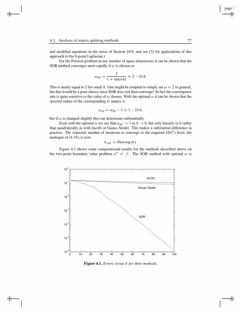
“rjlfdm”2007/6/1page 77✐
✐✐
✐
✐✐
✐✐
4.2. Analysis of matrix splitting methods 77
and modified equations in the sense of Section 10.9, and see [3] for applications of thisapproach to the 9-point Laplacian.)
For the Poisson problem in any number of space dimensions it can be shown that theSOR method converges most rapidly if ! is chosen as
!opt D 2
1 C sin.!h/! 2 " 2!h:
This is nearly equal to 2 for small h. One might be tempted to simply set ! D 2 in general,but this would be a poor choice since SOR does not then converge! In fact the convergencerate is quite sensitive to the value of ! chosen. With the optimal ! it can be shown that thespectral radius of the corresponding G matrix is
"opt D !opt " 1 ! 1 " 2!h;
but if ! is changed slightly this can deteriorate substantially.Even with the optimal ! we see that "opt ! 1 as h ! 0, but only linearly in h rather
than quadratically as with Jacobi or Gauss–Seidel. This makes a substantial difference inpractice. The expected number of iterations to converge to the required O.h2/ level, theanalogue of (4.19), is now
kopt D O.m log m/:
Figure 4.1 shows some computational results for the methods described above onthe two-point boundary value problem u00 D f . The SOR method with optimal ! is
0 10 20 30 40 50 60 70 80 90 10010
−6
10−5
10−4
10−3
10−2
10−1
100
SOR
Jacobi
Gauss−Seidel
Figure 4.1. Errors versus k for three methods.
“rjlfdm”2007/6/1page 78✐
✐✐
✐
✐✐
✐✐
78 Chapter 4. Iterative Methods for Sparse Linear Systems
far superior to Gauss–Seidel or Jacobi, at least for this simple problem with a symmetriccoefficient matrix. For more complicated problems it can be difficult to estimate the optimal!, however, and other approaches are usually preferred.
4.3 Descent methods and conjugate gradientsThe CG method is a powerful technique for solving linear systems Au D f when thematrix A is SPD, or negative definite since negating the system then gives an SPD matrix.This may seem like a severe restriction, but SPD methods arise naturally in many applica-tions, such as the discretization of elliptic equations. There are several ways to introducethe CG method and the reader may wish to consult texts such as [39], [79], [91] for otherapproaches and more analysis. Here the method is first motivated as a descent method forsolving a minimization problem.
Consider the function ! W Rm ! R defined by
!.u/ D 1
2uT Au ! uT f: (4.25)
This is a quadratic function of the variables u1; : : : ; um. For example, if m D 2, then
!.u/ D !.u1;u2/ D 1
2.a11u2
1 C 2a12u1u2 C a22u22/ ! u1f1 ! u2f2:
Note that since A is symmetric, a21 D a12. If A is positive definite, then plotting !.u/ asa function of u1 and u2 gives a parabolic bowl as shown in Figure 4.2(a). There is a uniquevalue u! that minimizes !.u/ over all choices of u. At the minimum, the partial derivativeof ! with respect to each component of u is zero, which gives the equations
@!
@u1D a11u1 C a12u2 ! f1 D 0;
@!
@u2D a21u1 C a22u2 ! f2 D 0:
(4.26)
This is exactly the linear system Au D f that we wish to solve. So finding u! that solvesthis system can equivalently be approached as finding u! to minimize !.u/. This is truemore generally when u 2 Rm and A 2 Rm"m is SPD. The function !.u/ in (4.25) has aunique minimum at the point u!, where r!.u!/ D 0, and
r!.u/ D Au ! f; (4.27)
so the minimizer solves the linear system Au D f .If A is negative definite, then !.u/ instead has a unique maximum at u!, which
again solves the linear system. If A is indefinite (neither positive nor negative definite),i.e., if the eigenvalues of A are not all of the same sign, then the function !.u/ still has astationary point with r!.u!/ D 0 at the solution to Au D f , but this is a saddle pointrather than a minimum or maximum, as illustrated in Figure 4.2(b). It is much harder tofind a saddle point than a minimum. An iterative method can find a minimum by alwaysheading downhill, but if we are looking for a saddle point, it is hard to tell if we need to
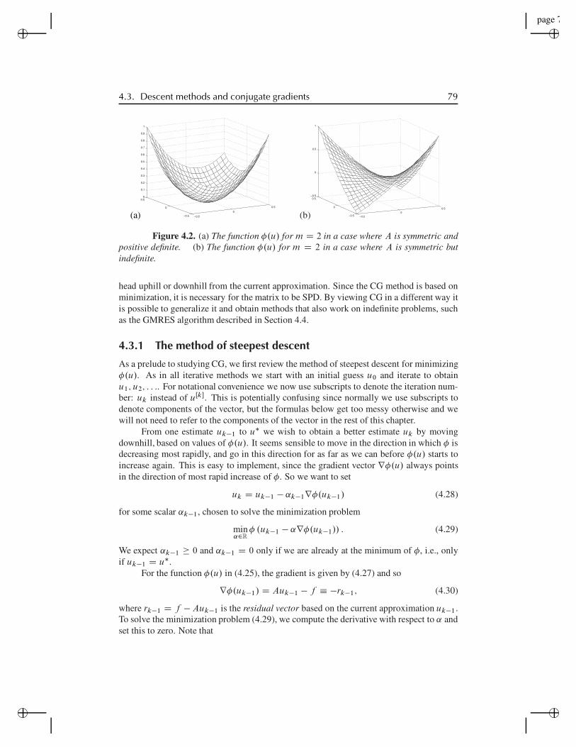
“rjlfdm”2007/6/1page 79✐
✐✐
✐
✐✐
✐✐
4.3. Descent methods and conjugate gradients 79
(a) −0.5
0
0.5
−0.5
0
0.50
0.1
0.2
0.3
0.4
0.5
0.6
0.7
0.8
0.9
1
(b) −0.50
0.5
−0.5
0
0.5−0.5
0
0.5
1
Figure 4.2. (a) The function !.u/ for m D 2 in a case where A is symmetric andpositive definite. (b) The function !.u/ for m D 2 in a case where A is symmetric butindefinite.
head uphill or downhill from the current approximation. Since the CG method is based onminimization, it is necessary for the matrix to be SPD. By viewing CG in a different way itis possible to generalize it and obtain methods that also work on indefinite problems, suchas the GMRES algorithm described in Section 4.4.
4.3.1 The method of steepest descentAs a prelude to studying CG, we first review the method of steepest descent for minimizing!.u/. As in all iterative methods we start with an initial guess u0 and iterate to obtainu1;u2; : : :. For notational convenience we now use subscripts to denote the iteration num-ber: uk instead of uŒk!. This is potentially confusing since normally we use subscripts todenote components of the vector, but the formulas below get too messy otherwise and wewill not need to refer to the components of the vector in the rest of this chapter.
From one estimate uk!1 to u" we wish to obtain a better estimate uk by movingdownhill, based on values of !.u/. It seems sensible to move in the direction in which ! isdecreasing most rapidly, and go in this direction for as far as we can before !.u/ starts toincrease again. This is easy to implement, since the gradient vector r!.u/ always pointsin the direction of most rapid increase of !. So we want to set
uk D uk!1 ! ˛k!1r!.uk!1/ (4.28)
for some scalar ˛k!1, chosen to solve the minimization problem
min˛2R
! .uk!1 ! ˛r!.uk!1// : (4.29)
We expect ˛k!1 " 0 and ˛k!1 D 0 only if we are already at the minimum of !, i.e., onlyif uk!1 D u".
For the function !.u/ in (4.25), the gradient is given by (4.27) and so
r!.uk!1/ D Auk!1 ! f # !rk!1; (4.30)
where rk!1 D f !Auk!1 is the residual vector based on the current approximation uk!1.To solve the minimization problem (4.29), we compute the derivative with respect to ˛ andset this to zero. Note that
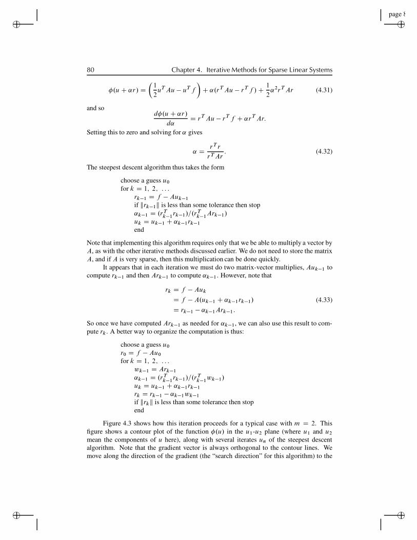
“rjlfdm”2007/6/1page 80✐
✐✐
✐
✐✐
✐✐
80 Chapter 4. Iterative Methods for Sparse Linear Systems
!.u C ˛r / D!
1
2uT Au ! uT f
"C ˛.r T Au ! r T f /C 1
2˛2r T Ar (4.31)
and sod!.u C ˛r /
d˛D r T Au ! r T f C ˛r T Ar:
Setting this to zero and solving for ˛ gives
˛ D r T r
r T Ar: (4.32)
The steepest descent algorithm thus takes the form
choose a guess u0
for k D 1; 2; : : :rk!1 D f ! Auk!1
if krk!1k is less than some tolerance then stop˛k!1 D .r T
k!1rk!1/=.r
Tk!1
Ark!1/uk D uk!1 C ˛k!1rk!1
end
Note that implementing this algorithm requires only that we be able to multiply a vector byA, as with the other iterative methods discussed earlier. We do not need to store the matrixA, and if A is very sparse, then this multiplication can be done quickly.
It appears that in each iteration we must do two matrix-vector multiplies, Auk!1 tocompute rk!1 and then Ark!1 to compute ˛k!1. However, note that
rk D f ! Auk
D f ! A.uk!1 C ˛k!1rk!1/
D rk!1 ! ˛k!1Ark!1:
(4.33)
So once we have computed Ark!1 as needed for ˛k!1, we can also use this result to com-pute rk . A better way to organize the computation is thus:
choose a guess u0
r0 D f ! Au0
for k D 1; 2; : : :wk!1 D Ark!1
˛k!1 D .r Tk!1
rk!1/=.rTk!1
wk!1/uk D uk!1 C ˛k!1rk!1
rk D rk!1 ! ˛k!1wk!1
if krkk is less than some tolerance then stopend
Figure 4.3 shows how this iteration proceeds for a typical case with m D 2. Thisfigure shows a contour plot of the function !.u/ in the u1-u2 plane (where u1 and u2
mean the components of u here), along with several iterates un of the steepest descentalgorithm. Note that the gradient vector is always orthogonal to the contour lines. Wemove along the direction of the gradient (the “search direction” for this algorithm) to the
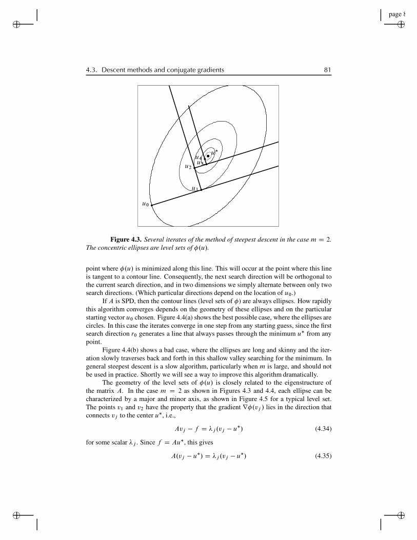
“rjlfdm”2007/6/1page 81✐
✐✐
✐
✐✐
✐✐
4.3. Descent methods and conjugate gradients 81
u!
u0
u1
u2u3
u4
Figure 4.3. Several iterates of the method of steepest descent in the case m D 2.The concentric ellipses are level sets of !.u/.
point where !.u/ is minimized along this line. This will occur at the point where this lineis tangent to a contour line. Consequently, the next search direction will be orthogonal tothe current search direction, and in two dimensions we simply alternate between only twosearch directions. (Which particular directions depend on the location of u0.)
If A is SPD, then the contour lines (level sets of !) are always ellipses. How rapidlythis algorithm converges depends on the geometry of these ellipses and on the particularstarting vector u0 chosen. Figure 4.4(a) shows the best possible case, where the ellipses arecircles. In this case the iterates converge in one step from any starting guess, since the firstsearch direction r0 generates a line that always passes through the minimum u! from anypoint.
Figure 4.4(b) shows a bad case, where the ellipses are long and skinny and the iter-ation slowly traverses back and forth in this shallow valley searching for the minimum. Ingeneral steepest descent is a slow algorithm, particularly when m is large, and should notbe used in practice. Shortly we will see a way to improve this algorithm dramatically.
The geometry of the level sets of !.u/ is closely related to the eigenstructure ofthe matrix A. In the case m D 2 as shown in Figures 4.3 and 4.4, each ellipse can becharacterized by a major and minor axis, as shown in Figure 4.5 for a typical level set.The points v1 and v2 have the property that the gradient r!.vj / lies in the direction thatconnects vj to the center u!, i.e.,
Avj ! f D "j .vj ! u!/ (4.34)
for some scalar "j . Since f D Au!, this gives
A.vj ! u!/ D "j .vj ! u!/ (4.35)
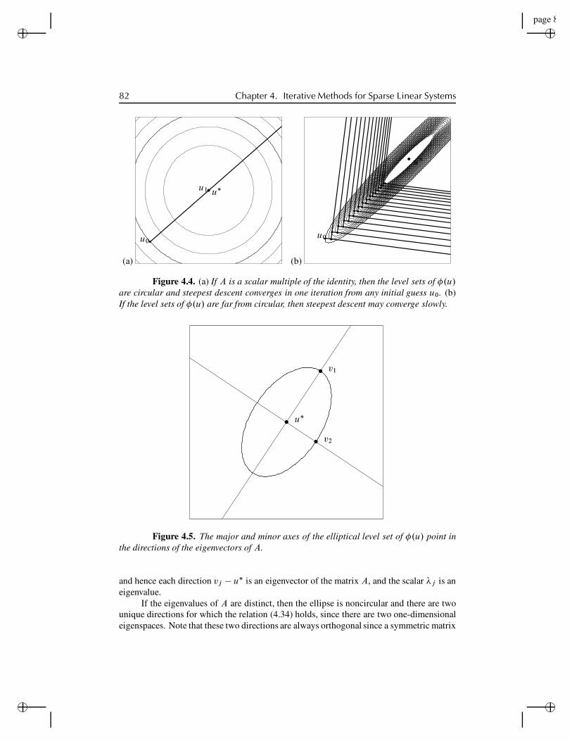
“rjlfdm”2007/6/1page 82✐
✐✐
✐
✐✐
✐✐
82 Chapter 4. Iterative Methods for Sparse Linear Systems
(a)
u!
u0
u1
(b)
u!
u0
Figure 4.4. (a) If A is a scalar multiple of the identity, then the level sets of !.u/are circular and steepest descent converges in one iteration from any initial guess u0. (b)If the level sets of !.u/ are far from circular, then steepest descent may converge slowly.
u!
v2
v1
Figure 4.5. The major and minor axes of the elliptical level set of !.u/ point inthe directions of the eigenvectors of A.
and hence each direction vj ! u! is an eigenvector of the matrix A, and the scalar "j is aneigenvalue.
If the eigenvalues of A are distinct, then the ellipse is noncircular and there are twounique directions for which the relation (4.34) holds, since there are two one-dimensionaleigenspaces. Note that these two directions are always orthogonal since a symmetric matrix
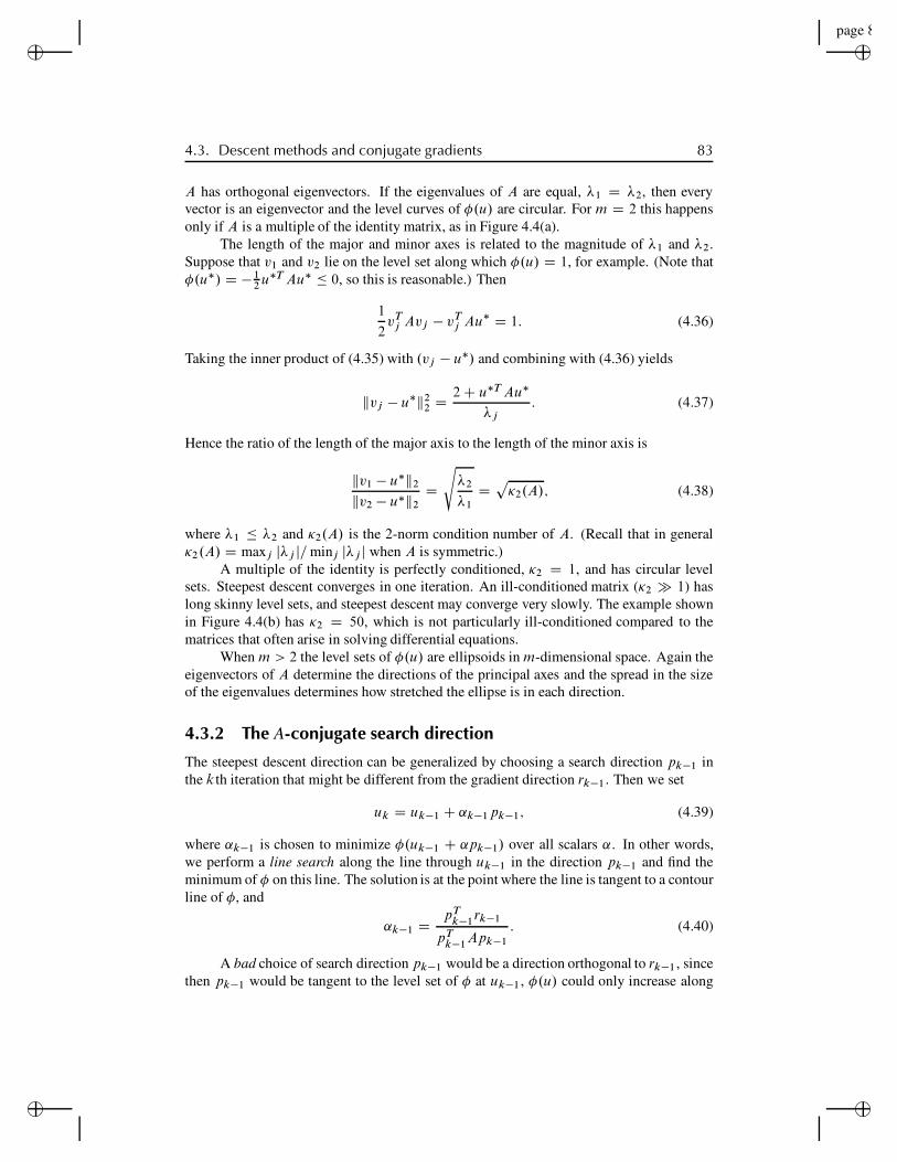
“rjlfdm”2007/6/1page 83✐
✐✐
✐
✐✐
✐✐
4.3. Descent methods and conjugate gradients 83
A has orthogonal eigenvectors. If the eigenvalues of A are equal, !1 D !2, then everyvector is an eigenvector and the level curves of ".u/ are circular. For m D 2 this happensonly if A is a multiple of the identity matrix, as in Figure 4.4(a).
The length of the major and minor axes is related to the magnitude of !1 and !2.Suppose that v1 and v2 lie on the level set along which ".u/ D 1, for example. (Note that".u!/ D !1
2 u!T Au! " 0, so this is reasonable.) Then
1
2vT
j Avj ! vTj Au! D 1: (4.36)
Taking the inner product of (4.35) with .vj ! u!/ and combining with (4.36) yields
kvj ! u!k22 D 2 C u!T Au!
!j: (4.37)
Hence the ratio of the length of the major axis to the length of the minor axis is
kv1 ! u!k2
kv2 ! u!k2Ds
!2
!1Dp#2.A/; (4.38)
where !1 " !2 and #2.A/ is the 2-norm condition number of A. (Recall that in general#2.A/ D maxj j!j j=minj j!j j when A is symmetric.)
A multiple of the identity is perfectly conditioned, #2 D 1, and has circular levelsets. Steepest descent converges in one iteration. An ill-conditioned matrix (#2 # 1) haslong skinny level sets, and steepest descent may converge very slowly. The example shownin Figure 4.4(b) has #2 D 50, which is not particularly ill-conditioned compared to thematrices that often arise in solving differential equations.
When m > 2 the level sets of ".u/ are ellipsoids in m-dimensional space. Again theeigenvectors of A determine the directions of the principal axes and the spread in the sizeof the eigenvalues determines how stretched the ellipse is in each direction.
4.3.2 The A-conjugate search directionThe steepest descent direction can be generalized by choosing a search direction pk"1 inthe kth iteration that might be different from the gradient direction rk"1. Then we set
uk D uk"1 C ˛k"1pk"1; (4.39)
where ˛k"1 is chosen to minimize ".uk"1 C ˛pk"1/ over all scalars ˛. In other words,we perform a line search along the line through uk"1 in the direction pk"1 and find theminimum of " on this line. The solution is at the point where the line is tangent to a contourline of ", and
˛k"1 DpT
k"1rk"1
pTk"1
Apk"1
: (4.40)
A bad choice of search direction pk"1 would be a direction orthogonal to rk"1, sincethen pk"1 would be tangent to the level set of " at uk"1, ".u/ could only increase along
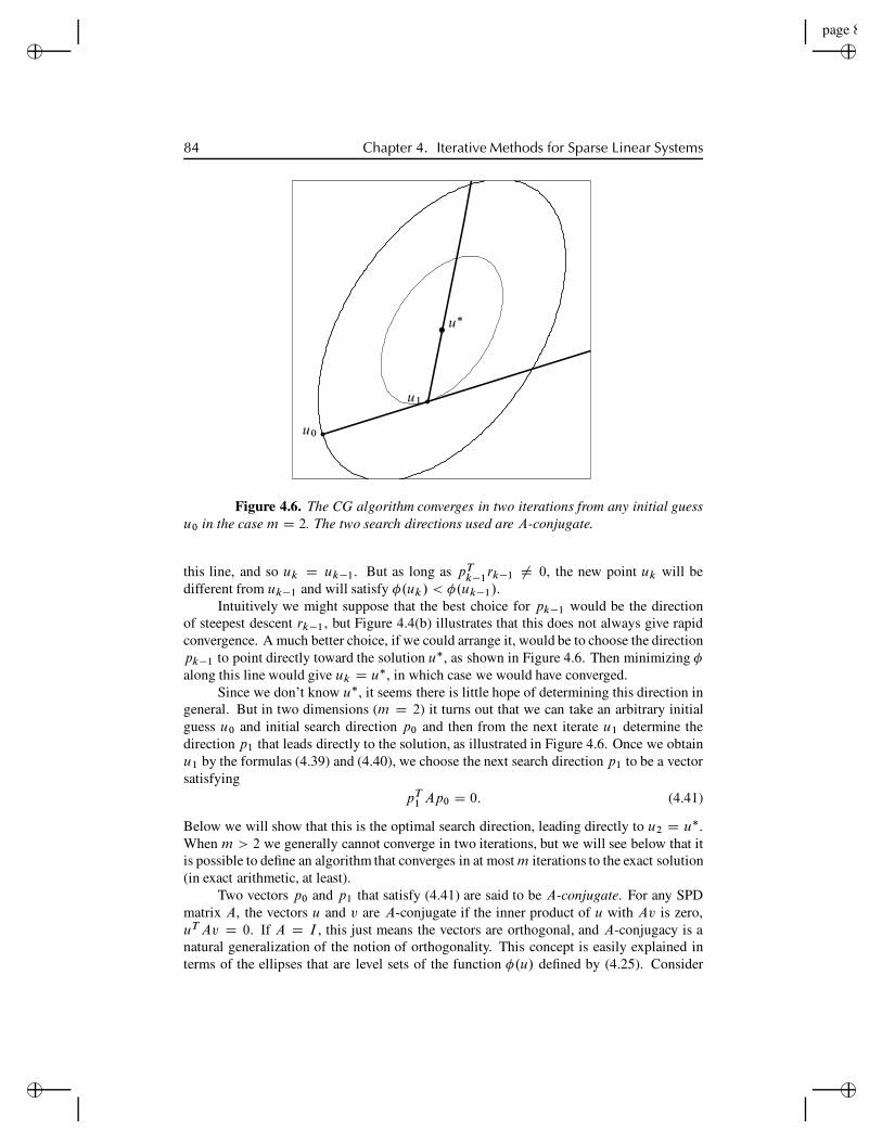
“rjlfdm”2007/6/1page 84✐
✐✐
✐
✐✐
✐✐
84 Chapter 4. Iterative Methods for Sparse Linear Systems
u0
u1
u!
Figure 4.6. The CG algorithm converges in two iterations from any initial guessu0 in the case m D 2. The two search directions used are A-conjugate.
this line, and so uk D uk"1. But as long as pTk"1
rk"1 ¤ 0, the new point uk will bedifferent from uk"1 and will satisfy !.uk / < !.uk"1/.
Intuitively we might suppose that the best choice for pk"1 would be the directionof steepest descent rk"1, but Figure 4.4(b) illustrates that this does not always give rapidconvergence. A much better choice, if we could arrange it, would be to choose the directionpk"1 to point directly toward the solution u!, as shown in Figure 4.6. Then minimizing !along this line would give uk D u!, in which case we would have converged.
Since we don’t know u!, it seems there is little hope of determining this direction ingeneral. But in two dimensions (m D 2) it turns out that we can take an arbitrary initialguess u0 and initial search direction p0 and then from the next iterate u1 determine thedirection p1 that leads directly to the solution, as illustrated in Figure 4.6. Once we obtainu1 by the formulas (4.39) and (4.40), we choose the next search direction p1 to be a vectorsatisfying
pT1 Ap0 D 0: (4.41)
Below we will show that this is the optimal search direction, leading directly to u2 D u!.When m > 2 we generally cannot converge in two iterations, but we will see below that itis possible to define an algorithm that converges in at most m iterations to the exact solution(in exact arithmetic, at least).
Two vectors p0 and p1 that satisfy (4.41) are said to be A-conjugate. For any SPDmatrix A, the vectors u and v are A-conjugate if the inner product of u with Av is zero,uT Av D 0. If A D I , this just means the vectors are orthogonal, and A-conjugacy is anatural generalization of the notion of orthogonality. This concept is easily explained interms of the ellipses that are level sets of the function !.u/ defined by (4.25). Consider
“rjlfdm”2007/6/1page 85✐
✐✐
✐
✐✐
✐✐
4.3. Descent methods and conjugate gradients 85
an arbitrary point on an ellipse. The direction tangent to the ellipse at this point and thedirection that points toward the center of the ellipse are always A-conjugate. This is thefact that allows us to determine the direction toward the center once we know a tangentdirection, which has been achieved by the line search in the first iteration. If A D I thenthe ellipses are circles and the direction toward the center is simply the radial direction,which is orthogonal to the tangent direction.
To prove that the two directions shown in Figure 4.6 are A-conjugate, note that thedirection p0 is tangent to the level set of ! at u1 and so p0 is orthogonal to the residualr1 D f ! Au1 D A.u! ! u1/, which yields
pT0 A.u! ! u1/ D 0: (4.42)
On the other hand, u! ! u1 D ˛p1 for some scalar ˛ ¤ 0 and using this in (4.42) gives(4.41).
Now consider the case m D 3, from which the essential features of the generalalgorithm will be more apparent. In this case the level sets of the function !.u/ are con-centric ellipsoids, two-dimensional surfaces in R3 for which the cross section in any two-dimensional plane is an ellipse. We start at an arbitrary point u0 and choose a searchdirection p0 (typically p0 D r0, the residual at u0). We minimize !.u/ along the one-dimensional line u0 C ˛p0, which results in the choice (4.40) for ˛0, and we set u1 Du0 C ˛0p0. We now choose the search direction p1 to be A-conjugate to p0. In the pre-vious example with m D 2 this determined a unique direction, which pointed straight tou!. With m D 3 there is a two-dimensional space of vectors p1 that are A-conjugate to p0
(the plane orthogonal to the vector Ap0). In the next section we will discuss the full CGalgorithm, where a specific choice is made that is computationally convenient, but for themoment suppose p1 is any vector that is both A-conjugate to p0 and also linearly indepen-dent from p0. We again use (4.40) to determine ˛1 so that u2 D u1 C ˛1p1 minimizes!.u/ along the line u1 C ˛p1.
We now make an observation that is crucial to understanding the CG algorithm forgeneral m. The two vectors p0 and p1 are linearly independent and so they span a planethat cuts through the ellipsoidal level sets of !.u/, giving a set of concentric ellipses thatare the contour lines of !.u/ within this plane. The fact that p0 and p1 are A-conjugatemeans that the point u2 lies at the center of these ellipses. In other words, when restrictedto this plane the algorithm so far looks exactly like the m D 2 case illustrated in Figure 4.6.
This means that u2 not only minimizes !.u/ over the one-dimensional line u1 C˛p1
but in fact minimizes !.u/ over the entire two-dimensional plane u0 C ˛p0 C ˇp1 for allchoices of ˛ and ˇ (with the minimum occurring at ˛ D ˛0 and ˇ D ˛1).
The next step of the algorithm is to choose a new search direction p2 that is A-conjugate to both p0 and p1. It is important that it be A-conjugate to both the previousdirections, not just the most recent direction. This defines a unique direction (the lineorthogonal to the plane spanned by Ap0 and Ap1). We now minimize !.u/ over the lineu2 C ˛p2 to obtain u3 D u2 C ˛2p2 (with ˛2 given by (4.40)). It turns out that thisalways gives u3 D u!, the center of the ellipsoids and the solution to our original problemAu D f .
In other words, the direction p2 always points from u2 directly through the center ofthe concentric ellipsoids. This follows from the three-dimensional version of the result weshowed above in two dimensions, that the direction tangent to an ellipse and the direction

“rjlfdm”2007/6/1page 86✐
✐✐
✐
✐✐
✐✐
86 Chapter 4. Iterative Methods for Sparse Linear Systems
toward the center are always A-conjugate. In the three-dimensional case we have a planespanned by p0 and p1 and the point u2 that minimized !.u/ over this plane. This planemust be the tangent plane to the level set of !.u/ through u2. This tangent plane is alwaysA-conjugate to the line connecting u2 to u! .
Another way to interpret this process is the following. After one step, u1 minimizes!.u/ over the one-dimensional line u0 C ˛p0. After two steps, u2 minimizes !.u/ overthe two-dimensional plane u0 C˛p0 Cˇp1. After three steps, u3 minimizes !.u/ over thethree-dimensional space u0 C ˛p0 C ˇp1 C "p2. But this is all of R3 (provided p0; p1,and p2 are linearly independent) and so u3 D u0 C ˛0p0 C ˛1p1 C ˛2p2 must be theglobal minimizer u!.
For m D 3 this procedure always converges in at most three iterations (in exactarithmetic, at least). It may converge to u! in fewer iterations. For example, if we happento choose an initial guess u0 that lies along one of the axes of the ellipsoids, then r0 willalready point directly toward u! , and so u1 D u! (although this is rather unlikely).
However, there are certain matrices A for which it will always take fewer iterationsno matter what initial guess we choose. For example, if A is a multiple of the identitymatrix, then the level sets of !.u/ are concentric circles. In this case r0 points toward u!
from any initial guess u0 and we always obtain convergence in one iteration. Note that inthis case all three eigenvalues of A are equal, #1 D #2 D #3.
In the “generic” case (i.e., a random SPD matrix A), all the eigenvalues of A aredistinct and three iterations are typically required. An intermediate case is if there are onlytwo distinct eigenvalues, e.g., #1 D #2 ¤ #3. In this case the level sets of ! appear circularwhen cut by certain planes but appear elliptical when cut at other angles. As we mightsuspect, it can be shown that the CG algorithm always converges in at most two iterationsin this case, from any initial u0.
This generalizes to the following result for the analogous algorithm in m dimensions:in exact arithmetic, an algorithm based on A-conjugate search directions as discussed aboveconverges in at most n iterations, where n is the number of distinct eigenvalues of the matrixA 2 Rm"m .n ! m/.
4.3.3 The conjugate-gradient algorithmIn the above description of algorithms based on A-conjugate search directions we requiredthat each search direction pk be A-conjugate to all previous search directions, but we didnot make a specific choice for this vector. In this section the full “conjugate gradient al-gorithm” is presented, in which a specific recipe for each pk is given that has very niceproperties both mathematically and computationally. The CG method was first proposedin 1952 by Hestenes and Stiefel [46], but it took some time for this and related methods tobe fully understood and widely used. See Golub and O’Leary [36] for some history of theearly developments.
This method has the feature mentioned at the end of the previous section: it alwaysconverges to the exact solution of Au D f in a finite number of iterations n ! m (inexact arithmetic). In this sense it is not really an iterative method mathematically. We canview it as a “direct method” like Gaussian elimination, in which a finite set of operationsproduces the exact solution. If we programmed it to always take m iterations, then inprinciple we would always obtain the solution, and with the same asymptotic work estimate
“rjlfdm”2007/6/1page 87✐
✐✐
✐
✐✐
✐✐
4.3. Descent methods and conjugate gradients 87
as for Gaussian elimination (since each iteration takes at most O.m2/ operations for matrix-vector multiplies, giving O.m3/ total work). However, there are two good reasons why CGis better viewed as an iterative method than a direct method:
! In theory it produces the exact solution in n iterations (where n is the number of dis-tinct eigenvalues) but in finite precision arithmetic un will not be the exact solution,and may not be substantially better than un!1. Hence it is not clear that the algorithmconverges at all in finite precision arithmetic, and the full analysis of this turns out tobe quite subtle [39].
! On the other hand, in practice CG frequently “converges” to a sufficiently accurateapproximation to u" in far less than n iterations. For example, consider solving aPoisson problem using the 5-point Laplacian on a 100 " 100 grid, which gives alinear system of dimension m D 10;000 and a matrix A that has n # 5000 dis-tinct eigenvalues. An approximation to u" consistent with the truncation error ofthe difference formula is obtained after approximately 150 iterations, however (afterpreconditioning the matrix appropriately).
That effective convergence often is obtained in far fewer iterations is crucial to thesuccess and popularity of CG, since the operation count of Gaussian elimination is far toolarge for most sparse problems and we wish to use an iterative method that is much quicker.To obtain this rapid convergence it is often necessary to precondition the matrix, whicheffectively moves the eigenvalues around so that they are distributed more conducively forrapid convergence. This is discussed in Section 4.3.5, but first we present the basic CGalgorithm and explore its convergence properties more fully.
The CG algorithm takes the following form:
Choose initial guess u0 (possibly the zero vector)r0 D f $ Au0
p0 D r0
for k D 1; 2; : : :wk!1 D Apk!1
˛k!1 D .r Tk!1
rk!1/=.pTk!1
wk!1/uk D uk!1 C ˛k!1pk!1
rk D rk!1 $ ˛k!1wk!1
if krkk is less than some tolerance then stopˇk!1 D .r T
krk/=.r
Tk!1
rk!1/pk D rk C ˇk!1pk!1
end
As with steepest descent, only one matrix-vector multiply is required at each iterationin computing wk!1. In addition, two inner products must be computed each iteration.(By more careful coding than above, the inner product of each residual with itself can becomputed once and reused twice.) To arrange this, we have used the fact that
pTk!1rk!1 D r T
k!1rk!1
to rewrite the expression (4.40).
“rjlfdm”2007/6/1page 88✐
✐✐
✐
✐✐
✐✐
88 Chapter 4. Iterative Methods for Sparse Linear Systems
Compare this algorithm to the steepest descent algorithm presented on page 80. Upthrough the convergence check it is essentially the same except that the A-conjugate searchdirection pk!1 is used in place of the steepest descent search direction rk!1 in severalplaces.
The final two lines in the loop determine the next search direction pk . This simplechoice gives a direction pk with the required property that pk is A-conjugate to all theprevious search directions pj for j D 0; 1; ; : : : ; k ! 1. This is part of the followingtheorem, which is similar to Theorem 38.1 of Trefethen and Bau [91], although there it isassumed that u0 D 0. See also Theorem 2.3.2 in Greenbaum [39].
Theorem 4.1. The vectors generated in the CG algorithm have the following properties,provided rk ¤ 0 (if rk D 0, then we have converged):
1. pk is A-conjugate to all the previous search directions, i.e., pTk
Apj D 0 for j D0; 1; ; : : : ; k ! 1.
2. The residual rk is orthogonal to all previous residuals, r Tk
rj D 0 for j D 0; 1; ; : : : ;k ! 1.
3. The following three subspaces of Rm are identical:
span.p0; p1; p2; : : : ; pk!1/;
span.r0; Ar0; A2r0; : : : ; Ak!1r0/;
span.Ae0; A2e0; A3e0; : : : ; Ak e0/:
(4.43)
The subspace Kk D span.r0; Ar0; A2r0; : : : ; Ak!1r0/ spanned by the vector r0
and the first k ! 1 powers of A applied to this vector is called a Krylov space of dimensionk associated with this vector.
The iterate uk is formed by adding multiples of the search directions pj to the initialguess u0 and hence must lie in the affine spaces u0 C Kk (i.e., the vector uk ! u0 is in thelinear space Kk).
We have seen that the CG algorithm can be interpreted as minimizing the function!.u/ over the space u0 C span.p0;p1; : : : ;pk!1/ in the kth iteration, and by the theoremabove this is equivalent to minimizing!.u/ over the u0CKk. Many other iterative methodsare also based on the idea of solving problems on an expanding sequence of Krylov spaces;see Section 4.4.
4.3.4 Convergence of conjugate gradientThe convergence theory for CG is related to the fact that uk minimizes !.u/ over the affinespace u0 C Kk defined in the previous section. We now show that a certain norm of theerror is also minimized over this space, which is useful in deriving estimates about the sizeof the error and rate of convergence.
Since A is assumed to be SPD, the A-norm defined by
kekA Dp
eT Ae (4.44)
“rjlfdm”2007/6/1page 89✐
✐✐
✐
✐✐
✐✐
4.3. Descent methods and conjugate gradients 89
satisfies the requirements of a vector norm in Section A.3, as discussed further in Sec-tion C.10. This is a natural norm to use because
kek2A D .u ! u!/T A.u ! u!/
D uT Au ! 2uT Au! C u!T Au!
D 2!.u/C u!T Au!:
(4.45)
Since u!T Au! is a fixed number, we see that minimizing kekA is equivalent to minimizing!.u/.
Sinceuk D u0 C ˛0p0 C ˛1p1 C " " " C ˛k"1pk"1;
we find by subtracting u! that
ek D e0 C ˛0p0 C ˛1p1 C " " "C ˛k"1pk"1:
Hence ek ! e0 is in Kk and by Theorem 4.1 lies in span.Ae0;A2e0; : : : ;A
ke0/. So ek De0 C c1Ae0 C c2A2e0 C " " "C ckAk e0 for some coefficients c1; : : : ; ck . In other words,
ek D Pk.A/e0; (4.46)
wherePk.A/ D I C c1A C c2A2 C " " "C ckAk (4.47)
is a polynomial in A. For a scalar value x we have
Pk.x/ D 1 C c1x C c2x2 C " " "C ckxk (4.48)
and Pk 2 Pk , where
Pk D fpolynomials P .x/ of degree at most k satisfying P .0/ D 1g: (4.49)
The polynomial Pk constructed implicitly by the CG algorithm solves the minimizationproblem
minP2Pk
kP .A/e0kA: (4.50)
To understand how a polynomial function of a diagonalizable matrix behaves, recall that
A D VƒV "1 H) Aj D Vƒj V "1;
where V is the matrix of right eigenvectors, and so
Pk.A/ D VPk .ƒ/V"1;
where
Pk.ƒ/ D
2
6664
Pk."1/Pk."2/
: : :
Pk."m/
3
7775:
“rjlfdm”2007/6/1page 90✐
✐✐
✐
✐✐
✐✐
90 Chapter 4. Iterative Methods for Sparse Linear Systems
Note, in particular, that if Pk.x/ has a root at each eigenvalue !1; : : : ; !m, then Pk.ƒ/is the zero matrix and so ek D Pk.A/e0 D 0. If A has only n ! m distinct eigenvalues!1; : : : ; !n, then there is a polynomial Pn 2 Pn that has these roots, and hence the CGalgorithm converges in at most n iterations, as was previously claimed.
To get an idea of how small ke0kA will be at some earlier point in the iteration, wewill show that for any polynomial P .x/ we have
kP .A/e0kA
ke0kA! max
1!j!mjP .!j /j (4.51)
and then exhibit one polynomial QPk 2 Pk for which we can use this to obtain a usefulupper bound on kekkA=ke0kk .
Since A is SPD, the eigenvectors are orthogonal and we can choose the matrix V sothat V "1 D V T and A D VƒV "1. In this case we obtain
kP .A/e0k2A D eT
0 P .A/T AP .A/e0
D eT0 VP .ƒ/V T AVP .ƒ/V T e0
D eT0 V diag.!j P .!j /
2/V T e0
! max1!j!m
P .!j /2!eT
0 VƒV T e0
":
(4.52)
Taking square roots and rearranging results in (4.51).We will now show that for a particular choice of polynomials QPk 2 Pk we can
evaluate the right-hand side of (4.51) and obtain a bound that decreases with increasing k .Since the polynomial Pk constructed by CG solves the problem (4.50), we know that
kPk.A/e0kA ! k QPk.A/e0kA;
and so this will give a bound for the convergence rate of the CG algorithm.Consider the case k D 1, after one step of CG. We choose the linear function
QP1.x/ D 1 " 2x
!m C !1; (4.53)
where we assume the eigenvalues are ordered 0 < !1 ! !2 ! # # # ! !m. A typical case isshown in Figure 4.7(a). The linear function QP1.x/ D 1Cc1x must pass through P1.0/ D 1and the slope c1 has been chosen so that
QP1.!1/ D " QP1.!m/;
which gives
1 C c1!1 D "1 " c1!m H) c1 D " 2
!m C !1:
If the slope were made any larger or smaller, then the value of j QP1.!/j would increase ateither !m or !1, respectively; see Figure 4.7(a). For this polynomial we have
max1!j!m
j QP1.!j /j D QP1.!1/ D 1 " 2!1
!m C !1D !m=!1 " 1
!m=!1 C 1
D " " 1
" C 1;
(4.54)
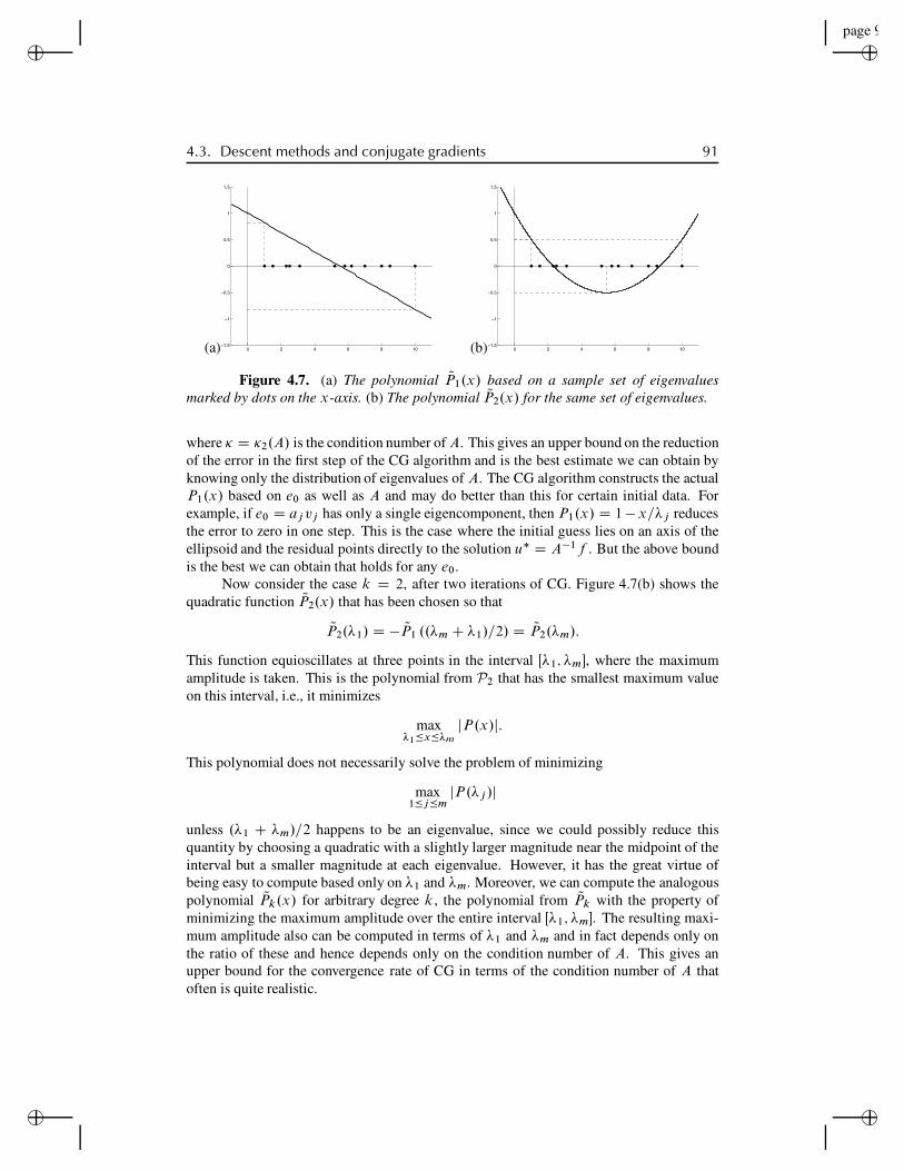
“rjlfdm”2007/6/1page 91✐
✐✐
✐
✐✐
✐✐
4.3. Descent methods and conjugate gradients 91
(a) 0 2 4 6 8 10−1.5
−1
−0.5
0
0.5
1
1.5
(b) 0 2 4 6 8 10−1.5
−1
−0.5
0
0.5
1
1.5
Figure 4.7. (a) The polynomial QP1.x/ based on a sample set of eigenvaluesmarked by dots on the x-axis. (b) The polynomial QP2.x/ for the same set of eigenvalues.
where ! D !2.A/ is the condition number of A. This gives an upper bound on the reductionof the error in the first step of the CG algorithm and is the best estimate we can obtain byknowing only the distribution of eigenvalues of A. The CG algorithm constructs the actualP1.x/ based on e0 as well as A and may do better than this for certain initial data. Forexample, if e0 D aj vj has only a single eigencomponent, then P1.x/ D 1!x="j reducesthe error to zero in one step. This is the case where the initial guess lies on an axis of theellipsoid and the residual points directly to the solution u! D A"1f . But the above boundis the best we can obtain that holds for any e0.
Now consider the case k D 2, after two iterations of CG. Figure 4.7(b) shows thequadratic function QP2.x/ that has been chosen so that
QP2."1/ D ! QP1 .."m C "1/=2/ D QP2."m/:
This function equioscillates at three points in the interval Œ"1;"m#, where the maximumamplitude is taken. This is the polynomial from P2 that has the smallest maximum valueon this interval, i.e., it minimizes
max!1#x#!m
jP .x/j:
This polynomial does not necessarily solve the problem of minimizing
max1#j#m
jP ."j /j
unless ."1 C "m/=2 happens to be an eigenvalue, since we could possibly reduce thisquantity by choosing a quadratic with a slightly larger magnitude near the midpoint of theinterval but a smaller magnitude at each eigenvalue. However, it has the great virtue ofbeing easy to compute based only on "1 and "m. Moreover, we can compute the analogouspolynomial QPk.x/ for arbitrary degree k , the polynomial from QPk with the property ofminimizing the maximum amplitude over the entire interval Œ"1;"m#. The resulting maxi-mum amplitude also can be computed in terms of "1 and "m and in fact depends only onthe ratio of these and hence depends only on the condition number of A. This gives anupper bound for the convergence rate of CG in terms of the condition number of A thatoften is quite realistic.
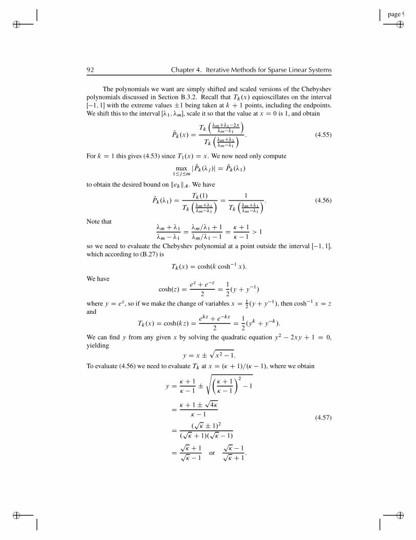
“rjlfdm”2007/6/1page 92✐
✐✐
✐
✐✐
✐✐
92 Chapter 4. Iterative Methods for Sparse Linear Systems
The polynomials we want are simply shifted and scaled versions of the Chebyshevpolynomials discussed in Section B.3.2. Recall that Tk.x/ equioscillates on the intervalŒ!1; 1! with the extreme values ˙1 being taken at k C 1 points, including the endpoints.We shift this to the interval Œ"1;"m!, scale it so that the value at x D 0 is 1, and obtain
QPk.x/ DTk
!!mC!1!2x
!m!!1
"
Tk
!!mC!1
!m!!1
" : (4.55)
For k D 1 this gives (4.53) since T1.x/ D x. We now need only compute
max1"j"m
j QPk."j /j D QPk."1/
to obtain the desired bound on kekkA. We have
QPk."1/ D Tk.1/
Tk
!!mC!1
!m!!1
" D 1
Tk
!!mC!1
!m!!1
" : (4.56)
Note that"m C "1
"m ! "1D "m="1 C 1
"m="1 ! 1D # C 1
# ! 1> 1
so we need to evaluate the Chebyshev polynomial at a point outside the interval Œ!1; 1!,which according to (B.27) is
Tk.x/ D cosh.k cosh!1 x/:
We have
cosh.z/ D ez C e!z
2D 1
2.y C y!1/
where y D ez, so if we make the change of variables x D 12.y C y!1/, then cosh!1 x D z
and
Tk.x/ D cosh.kz/ D ekz C e!kz
2D 1
2.yk C y!k /:
We can find y from any given x by solving the quadratic equation y2 ! 2xy C 1 D 0,yielding
y D x ˙p
x2 ! 1:
To evaluate (4.56) we need to evaluate Tk at x D .# C 1/=.# ! 1/, where we obtain
y D # C 1
# ! 1˙
s## C 1
# ! 1
$2
! 1
D # C 1 ˙p
4#
# ! 1
D .p# ˙ 1/2
.p# C 1/.
p# ! 1/
Dp# C 1p# ! 1
orp# ! 1p# C 1
:
(4.57)

“rjlfdm”2007/6/1page 93✐
✐✐
✐
✐✐
✐✐
4.3. Descent methods and conjugate gradients 93
Either choice of y gives the same value for
Tk
!! C 1
! ! 1
"D 1
2
"!p! C 1p! ! 1
"k
C!p
! ! 1p! C 1
"k#: (4.58)
Using this in (4.56) and combining with (4.51) gives
kP .A/e0kA
ke0kA" 2
"!p! C 1p! ! 1
"k
C!p
! ! 1p! C 1
"k#!1
" 2
!p! ! 1p! C 1
"k
: (4.59)
This gives an upper bound on the error when the CG algorithm is used. In practice theerror may be smaller, either because the initial error e0 happens to be deficient in someeigencoefficients or, more likely, because the optimal polynomial Pk.x/ is much smaller atall the eigenvalues "j than our choice QPk.x/ used to obtain the above bound. This typicallyhappens if the eigenvalues of A are clustered near fewer than m points. Then the Pk.x/constructed by CG will be smaller near these points and larger on other parts of the intervalŒ"1;"m# where no eigenvalues lie. As an iterative method it is really the number of clusters,not the number of mathematically distinct eigenvalues, that then determines how rapidlyCG converges in practical terms.
The bound (4.59) is realistic for many matrices, however, and shows that in generalthe convergence rate depends on the size of the condition number !. If ! is large, then
2
!p! ! 1p! C 1
"k
# 2
!1! 2p
!
"k
# 2e!2k=p
!; (4.60)
and we expect that the number of iterations required to reach a desired tolerance will bek D O.
p!/.
For example, the standard second order discretization of the Poisson problem ona grid with m points in each direction gives a matrix with ! D O.1=h2/, where h D1=.m C 1/. The bound (4.60) suggests that CG will require O.m/ iterations to converge,which is observed in practice. This is true in any number of space dimensions. In onedimension where there are only m unknowns this does not look very good (and of courseit’s best just to solve the tridiagonal system by elimination). In two dimensions there are m2
unknowns and m2 work per iteration is required to compute Apk!1, so CG requires O.m3/work to converge to a fixed tolerance, which is significantly better than Gauss eliminationand comparable to SOR with the optimal!. Of course for this problem a fast Poisson solvercould be used, requiring only O.m2 log m/ work. But for other problems, such as variablecoefficient elliptic equations with symmetric coefficient matrices, CG may still work verywell while SOR works well only if the optimal ! is found, which may be impossible, andfast Fourier transform (FFT) methods are inapplicable. Similar comments apply in threedimensions.
4.3.5 PreconditionersWe saw in Section 4.3.4 that the convergence rate of CG generally depends on the condi-tion number of the matrix A. Often preconditioning the system can reduce the condition
“rjlfdm”2007/6/1page 94✐
✐✐
✐
✐✐
✐✐
94 Chapter 4. Iterative Methods for Sparse Linear Systems
number of the matrix involved and speed up convergence. In fact preconditioning is abso-lutely essential for most practical problems, and there are many papers in the literature onthe development of effective preconditioners for specific applications or general classes ofproblems.
If M is any nonsingular matrix, then
Au D f () M !1Au D M !1f: (4.61)
So we could solve the system on the right instead of the system on the left. If M is someapproximation to A, then M !1A may have a much smaller condition number than A. IfM D A, then M !1A is perfectly conditioned but we’d still be faced with the problem ofcomputing M !1f D A!1f .
Of course in practice we don’t actually form the matrix M !1A. As we will seebelow, the preconditioned conjugate gradient (PCG) algorithm has the same basic formas CG, but a step is added in which a system of the form M z D r is solved, and it ishere that the preconditioner is “applied.” The idea is to choose an M for which M !1A isbetter conditioned than A but for which systems involving M are much easier to solve thansystems involving A. Often this can be done by solving some approximation to the originalphysical problem (e.g., by solving on a coarser grid and then interpolating, by solving anearby constant-coefficient problem).
A very simple preconditioner that is effective for some problems is simply to useM D diag(A), a diagonal matrix for which solving linear systems is trivial. This doesn’thelp for the Poisson problem on a rectangle, where this is just a multiple of the identitymatrix, and hence doesn’t change the condition number at all, but for other problems suchas variable coefficient elliptic equations with large variation in the coefficients, this canmake a significant difference.
Another popular approach is to use an incomplete Cholesky factorization of the ma-trix A, as discussed briefly in Section 4.3.6. Other iterative methods are sometimes usedas a preconditioner, for example, the multigrid algorithm of Section 4.6. Other precondi-tioners are discussed in many places; for example, there is a list of possible approaches inTrefethen and Bau [91].
A problem with the approach to preconditioning outlined above is that M !1A maynot be symmetric, even if M !1 and A are, in which case CG could not be applied to thesystem on the right in (4.61). Instead we can consider solving a different system, againequivalent to the original:
.C !T AC !1/.C u/ D C !T f; (4.62)
where C is a nonsingular matrix. Write this system as
QA Qu D Qf : (4.63)
Note that since AT D A, the matrix QA is also symmetric even if C is not. Moreover QA ispositive definite (provided A is) since
uT QAu D uT C !T AC !1u D .C !1u/T A.C !1u/ > 0
for any vector u ¤ 0.
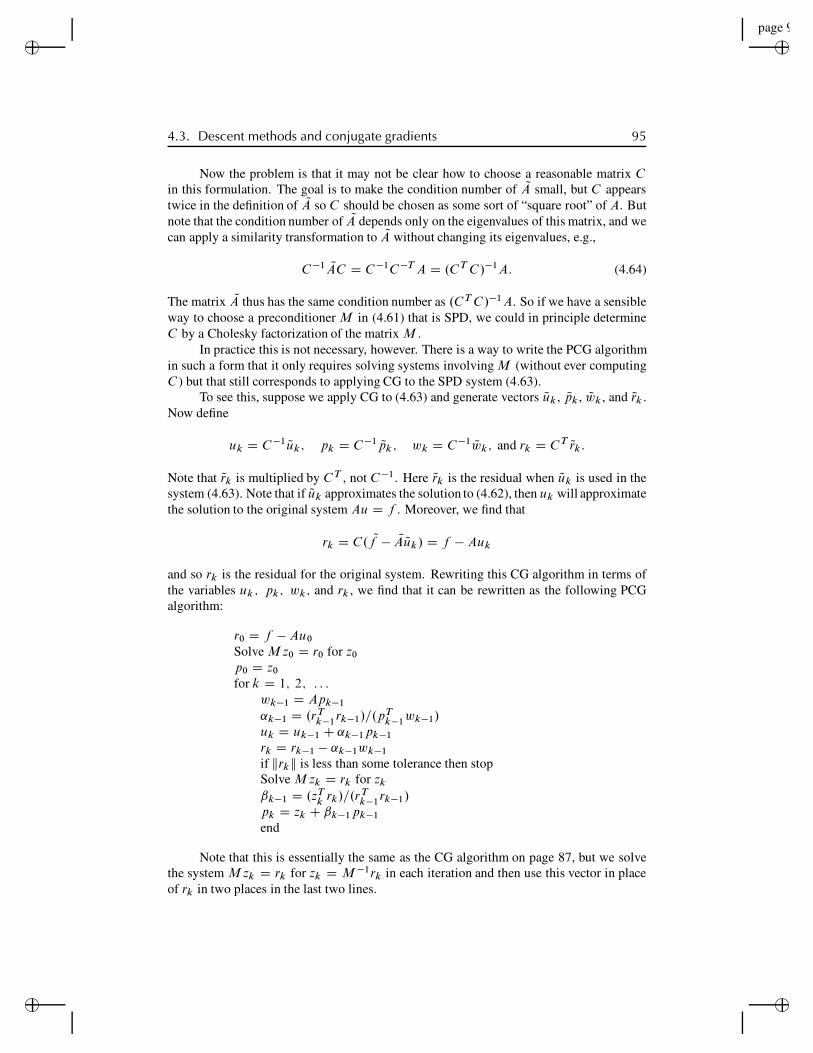
“rjlfdm”2007/6/1page 95✐
✐✐
✐
✐✐
✐✐
4.3. Descent methods and conjugate gradients 95
Now the problem is that it may not be clear how to choose a reasonable matrix Cin this formulation. The goal is to make the condition number of QA small, but C appearstwice in the definition of QA so C should be chosen as some sort of “square root” of A. Butnote that the condition number of QA depends only on the eigenvalues of this matrix, and wecan apply a similarity transformation to QA without changing its eigenvalues, e.g.,
C !1 QAC D C !1C !T A D .C T C /!1A: (4.64)
The matrix QA thus has the same condition number as .C T C /!1A. So if we have a sensibleway to choose a preconditioner M in (4.61) that is SPD, we could in principle determineC by a Cholesky factorization of the matrix M .
In practice this is not necessary, however. There is a way to write the PCG algorithmin such a form that it only requires solving systems involving M (without ever computingC ) but that still corresponds to applying CG to the SPD system (4.63).
To see this, suppose we apply CG to (4.63) and generate vectors Quk , Qpk , Qwk , and Qrk .Now define
uk D C !1 Quk ; pk D C !1 Qpk ; wk D C !1 Qwk ; and rk D C T Qrk :
Note that Qrk is multiplied by C T , not C !1. Here Qrk is the residual when Quk is used in thesystem (4.63). Note that if Quk approximates the solution to (4.62), then uk will approximatethe solution to the original system Au D f . Moreover, we find that
rk D C. Qf ! QA Quk / D f ! Auk
and so rk is the residual for the original system. Rewriting this CG algorithm in terms ofthe variables uk ; pk ; wk ; and rk , we find that it can be rewritten as the following PCGalgorithm:
r0 D f ! Au0
Solve M z0 D r0 for z0
p0 D z0
for k D 1; 2; : : :wk!1 D Apk!1
˛k!1 D .r Tk!1
rk!1/=.pTk!1
wk!1/uk D uk!1 C ˛k!1pk!1
rk D rk!1 ! ˛k!1wk!1
if krkk is less than some tolerance then stopSolve M zk D rk for zk
ˇk!1 D .zTk
rk/=.rTk!1
rk!1/pk D zk C ˇk!1pk!1
end
Note that this is essentially the same as the CG algorithm on page 87, but we solvethe system M zk D rk for zk D M !1rk in each iteration and then use this vector in placeof rk in two places in the last two lines.
“rjlfdm”2007/6/1page 96✐
✐✐
✐
✐✐
✐✐
96 Chapter 4. Iterative Methods for Sparse Linear Systems
4.3.6 Incomplete Cholesky and ILU preconditionersThere is one particular preconditioning strategy where the matrix C is in fact computed andused. Since A is SPD it has a Cholesky factorization of the form A D RT R, where R isan upper triangular matrix (this is just a special case of the LU factorization). The problemwith computing and using this factorization to solve the original system Au D f is thatthe elimination process used to compute R generates a lot of nonzeros in the R matrix, sothat it is typically much less sparse than A.
A popular preconditioner that is often very effective is to do an incomplete Choleskyfactorization of the matrix A, in which nonzeros in the factors are allowed to appear onlyin positions where the corresponding element of A is nonzero, simply throwing away theother elements as we go along. This gives an approximate factorization of the form A !C T C . This defines a preconditioner M D C T C . To solve systems of the form M z D rrequired in the PCG algorithm we use the known Cholesky factorization of M and onlyneed to do forward and back substitutions for these lower and upper triangular systems.This approach can be generalized by specifying a drop tolerance and dropping only thoseelements of R that are smaller than this tolerance. A smaller drop tolerance will give abetter approximation to A but a denser matrix C .
Methods for nonsymmetric linear systems (e.g., the GMRES algorithm in the nextsection) also generally benefit greatly from preconditioners and this idea can be extendedto incomplete LU (ILU) factorizations as a preconditioner for nonsymmetric systems.
4.4 The Arnoldi process and GMRES algorithmFor linear systems that are not SPD, many other iterative algorithms have been developed.We concentrate here on just one of these, the popular GMRES (generalized minimum resid-ual) algorithm. In the course of describing this method we will also see the Arnoldi process,which is useful in other applications.
In the kth step of GMRES a least squares problem is solved to find the best approx-imation to the solution of Au D f from the affine space u0 C Kk , where again Kk is thek-dimensional Krylov space Kk D span.r0;Ar0;A
2r0; : : : ;Ak!1r0/ based on the initial
residual r0 D f " Au0. To do this we build up a matrix of the form
Qk D Œq1 q2 # # # qk ! 2 Rm"k ;
whose columns form an orthonormal basis for the space Kk . In the kth iteration we deter-mine the vector qkC1 by starting with some vector vj that is not in Kk and orthogonalizingit to q1; q2; : : : ; qk using a Gram–Schmidt-type procedure. How should we choose vk?One obvious choice might be vk D Ak r0. This is a bad choice, however. The vectorsr0; Ar0; A2r0; : : :, although linearly independent and a natural choice from our defini-tion of the Krylov space, tend to become more and more closely aligned (nearly linearlydependent) as k grows. (In fact they converge to the eigenvector direction of the dominanteigenvalue of A since this is just the power method.) In other words the Krylov matrix
KkC1 D Œr0 Ar0 A2r0 # # # Ak r0!
has rank k C 1 but has some very small singular values. Applying the orthogonalizationprocedure using vk D Ak r0 would amount to doing a QR factorization of the matrix KkC1,
“rjlfdm”2007/6/1page 97✐
✐✐
✐
✐✐
✐✐
4.4. The Arnoldi process and GMRES algorithm 97
which is numerically unstable in this case. Moreover, it is not clear how we would usethe resulting basis to find the least square approximation to Au D f in the affine spaceu0 C Kk .
Instead we choose vk D Aqk as the starting point in the kth step. Since qk has al-ready been orthogonalized to all the previous basis vectors, this does not tend to be alignedwith an eigendirection. In addition, the resulting procedure can be viewed as building upa factorization of the matrix A itself that can be directly used to solve the desired leastsquares problem.
This procedure is called the Arnoldi process. This algorithm is important in otherapplications as well as in the solution of linear systems, as we will see below. Here isthe basic algorithm, with an indication of where a least squares problem should be solvedin each iteration to compute the GMRES approximations uk to the solution of the linearsystem:
q1 D r0=kr0k2
for k D 1; 2; : : :v D Aqk
for i D 1 W khik D qT
i vv D v ! hikqi % orthogonalize to previous vectorsend
hkC1;k D kvk2
qkC1 D v=hkC1;k % normalize% For GMRES: Check residual of least squares problem (4.75).% If it’s sufficiently small, halt and compute uk
end
Before discussing the least squares problem, we must investigate the form of thematrix factorization we are building up with this algorithm. After k iterations we have
Qk D Œq1 q2 " " " qk ! 2 Rm!k ; QkC1 D ŒQk qkC1! 2 Rm!.kC1/;
which form orthonormal bases for Kk and KkC1, respectively. Let
Hk D
2
666664
h11 h12 h13 " " " h1;k"1 h1k
h21 h22 h23 " " " h2;k"1 h2k
h32 h33 " " " h3;k"1 h3k
: : :: : :
:::hk;k"1 hkk
3
7777752 Rk!k (4.65)
be the upper Hessenberg matrix consisting of the h values computed so far. We will alsoneed the matrix QHk 2 R.kC1/!k consisting of Hk with an additional row that is all zerosexcept for the hkC1;k entry, also computed in the kth step of Arnoldi.
Now consider the matrix product
AQk D ŒAq1 Aq2 " " " Aqk !:

“rjlfdm”2007/6/1page 98✐
✐✐
✐
✐✐
✐✐
98 Chapter 4. Iterative Methods for Sparse Linear Systems
The j th column of this matrix has the form of the starting vector v used in the j th iterationof Arnoldi, and unraveling the computations done in the j th step shows that
hjC1;j qjC1 D Aqj ! h1j q1 ! h2j q2 ! " " " ! hjj qj :
This can be rearranged to give
Aqj D h1j q1 C h2j q2 C " " "C hjj qj C hjC1;j qjC1: (4.66)
The left-hand side is the j th column of AQk and the right-hand side, at least for j < k , isthe j th column of the matrix QkHk . We find that
AQk D QkHk C hkC1;k qkC1eTk : (4.67)
In the final term the vector eTk
D Œ0 0 " " " 0 1! is the vector of length k with a 1 in the lastcomponent and hkC1;k qkC1eT
kis the m # k matrix that is all zeros except the last column,
which is hkC1;k qkC1. This term corresponds to the last term in the expression (4.66) forj D k . The expression (4.67) can also be rewritten as
AQk D QkC1QHk : (4.68)
If we run the Arnoldi process to completion (i.e., up to k D m, the dimension ofA), then we will find in the final step that v D Aqm lies in the Krylov space Km (which isalready all of Rm), so orthogonalizing it to each of the qi for i D 1 W m will leave us withv D 0. So in this final step there is no hmC1;m value or qmC1 vector and setting Q D Qm
and H D Hm gives the resultAQ D QH;
which yieldsQT AQ D H or A D QHQT : (4.69)
We have reduced A to Hessenberg form by a similarity transformation.Our aim at the moment is not to reduce A all the way by running the algorithm to
k D m but rather to approximate the solution to Au D f well in a few iterations. After kiterations we have (4.67) holding. We wish to compute uk , an approximation to u D A!1ffrom the affine space u0 C Kk , by minimizing the 2-norm of the residual rk D f ! Auk
over this space. Since the columns of Qk form a basis for Kk , we must have
uk D u0 C Qk yk (4.70)
for some vector yk 2 Rk , and so the residual is
rk D f ! A.u0 C Qk yk /
D r0 ! AQk yk
D r0 ! QkC1QHk yk ;
(4.71)
where we have used (4.68). But recall that the first column of QkC1 is just q1 D r0=kr0k2
so we have r0 D QkC1", where " is the vector
" D
2
6664
kr0k2
0:::0
3
77752 RkC1: (4.72)
“rjlfdm”2007/6/1page 99✐
✐✐
✐
✐✐
✐✐
4.4. The Arnoldi process and GMRES algorithm 99
Hencerk D QkC1.! ! QHk yk /: (4.73)
Since QTkC1QkC1 D I , computing r T
k rk shows that
krkk2 D k!! QHk yk k2: (4.74)
In the kth iteration of GMRES we choose yk to solve the least squares problem
miny2Rk
k!! QHkyk2; (4.75)
and the approximation uk is then given by (4.70).Note the following (see, e.g., Greenbaum [39] for details):
" QHk 2 R.kC1/!k and ! 2 RkC1, so this is a small least squares problem when k # m.
" QHk is already nearly upper triangular, so solving the least squares problem by com-puting the QR factorization of this matrix is relatively cheap.
" Moreover, in each iteration QHk consists of QHk"1 with one additional row and columnadded. Since the QR factorization of QHk"1 has already been computed in the pre-vious iteration, the QR factorization of QHk is easily computed with little additionalwork.
" Once the QR factorization is known, it is possible to compute the residual in the leastsquares problem (4.75) without actually solving for yk (which requires solving anupper triangular system of size k using the R matrix from QR). So in practice onlythe residual is checked each iteration and the final yk and uk are actually computedonly after the convergence criterion is satisfied.
Notice, however, one drawback of GMRES, and the Arnoldi process more generally,for nonsymmetric matrices: in the kth iteration we must orthogonalize v to all k previ-ous basis vectors, so we must keep all these vectors in storage. For practical problemsarising from discretizing a multidimensional partial differential equation (PDE), each ofthese “vectors” is an approximation to the solution over the full grid, which may consistof millions of grid points. Taking more than a few iterations may consume a great deal ofstorage.
Often in GMRES the iteration is restarted periodically to save storage: the approxi-mation uk at some point is used as the initial guess for a new GMRES iteration. There’s alarge literature on this and other variations of GMRES.
4.4.1 Krylov methods based on three term recurrencesNote that if A is symmetric, then so is the Hessenberg matrix H , since
H T D .QT AQ/T D QT AT Q D QT AQ D H;
and hence H must be tridiagonal. In this case the Arnoldi iteration simplifies in a veryimportant way: hik D 0 for i D 1; 2; : : : ; .k ! 2/ and in the kth iteration of Arnoldi v
“rjlfdm”2007/6/1page 100✐
✐✐
✐
✐✐
✐✐
100 Chapter 4. Iterative Methods for Sparse Linear Systems
only needs to be orthogonalized to the previous two basis vectors. There is a three-termrecurrence relation for each new basis vector in terms of the previous two. This meansonly the two previous vectors need to be stored at any time, rather than all the previous qi
vectors, which is a dramatic improvement for systems of large dimension.The special case of Arnoldi on a symmetric matrix (or more generally a complex
Hermitian matrix) is called the Lanczos iteration and plays an important role in many nu-merical algorithms, not just for linear systems but also for eigenvalue problems and otherapplications.
There are also several iterative methods for nonsymmetric systems of equations thatare based on three-term recurrence relations using the idea of biorthogonalization—in ad-dition to building up a Krylov space based on powers of the matrix A, a second Krylovspace based on powers of the matrix AH is simultaneously determined. Basis vectors vi
and wi for the two spaces are found that are not orthogonal sets separately, but are instead“biorthogonal” in the sense that
vHi wj D 0 if i ¤ j:
It turns out that there are three-term recurrence relations for these sets of basis vectors,eliminating the need for storing long sequences of vectors. The disadvantage is that twomatrix-vector multiplies must be performed each iteration, one involving A and anotherinvolving AH . One popular method of this form is Bi-CGSTAB (bi-conjugate gradientstabilized), introduced by Van der Vorst [95]. See, e.g., [39], [91] for more discussion ofthis method and other variants.
4.4.2 Other applications of ArnoldiThe Arnoldi process has other applications besides the approximate solution of linear sys-tems. Note from (4.67) that
QTk AQk D Hk (4.76)
since QTk Qk D I and QT
k qkC1 D 0. This looks much like (4.69), but here Qk is a rectan-gular matrix (for k < m) and so this is not a similarity transformation and Hk does not havethe same eigenvalues as A (or even the same number of eigenvalues, since it has only k).However, a very useful fact is that the eigenvalues of Hk are typically good approximationsto the dominant eigenvalues of A (those with largest magnitude). In many eigenvalue appli-cations where A is a large sparse matrix, the primary interest is in determining the dominanteigenvalues (e.g., in determining stability or asymptotic growth properties of matrix iter-ations or exponentials). In this case we can run the Arnoldi process (which requires onlymatrix-vector multiplies with A) and then calculate the eigenvalues of the small matrix Hk
in the kth iteration as an approximation to the dominant eigenvalues of A. This approachis implemented in the ARPACK software [62], which is used, for example, by the eigscommand in MATLAB.
Also note that from (4.76), by multiplying on the left by Qk and on the right by QTk
we obtainQk QT
k AQkQTk D Qk HkQT
k : (4.77)
If k D m, then QkQTk
D I and this is simply (4.69). For k < m, QkQTk
is the pro-jection matrix that projects any vector z in Rm onto the k-dimensional Krylov space Kk .
“rjlfdm”2007/6/1page 101✐
✐✐
✐
✐✐
✐✐
4.5. Newton–Krylov methods for nonlinear problems 101
So the operator on the left of (4.77), when applied to any vector in z 2 Rm, has the fol-lowing effect: the vector is first projected to Kk , then A is applied, and then the resultis again projected to Kk . The operator on the right does the same thing in a differentform: QT
kz 2 Rk consists of the coefficients of the basis vectors of Qk for the projected
vector. Multiplying by Hk transforms these coefficients according to the effect of A, andHk QT
k z are then the modified coefficients used to form a linear combination of the basisvectors when this is multiplied by Qk . Hence we can view Hk as the restriction of A tothe k-dimensional Krylov space Kk . Thus it is not so surprising, for example, that theeigenvalues of Hk approximate the dominant eigenvalues of A. As commented above, thebasis vectors f; Af; A2f; : : : for Kk tend to align with the dominant eigenvectors of A,and if an eigenvector of A lies in Kk , then it is also an eigenvector of the restriction of Ato this space.
We will see another use of Krylov space methods in Section 11.6, where we considerexponential time differencing methods for time-dependent ordinary differential equations(ODEs). The matrix exponential applied to a vector, eAtv, arises in solving linear systemsof ODEs. This often can be effectively approximated by Qk eHktQT
kv for k ! m. More
generally, other functions !.z/ can be extended to matrix arguments (using the Cauchyintegral formula (D.4), for example) and their action often approximated by !.A/v "Qk!.Hk t/QT
kv.
4.5 Newton–Krylov methods for nonlinear problemsSo far in this chapter we have considered only linear problems and a variety of iterativemethods that can be used to solve sparse linear systems of the form Au D f . However,many differential equations are nonlinear and these naturally give rise to nonlinear systemsof equations after discretization. In Section 2.16 we considered a nonlinear boundary valueproblem and discussed the use of Newton’s method for its solution. Recall that Newton’smethod is an iterative method based on linearizing the problem about the current approxi-mation to the solution and then solving a linear system of equations involving the Jacobianmatrix to determine the next update to the approximation. If the nonlinear system is writtenas G.u/ D 0, then the Newton update is
uŒjC1! D uŒj ! # ıŒj !; (4.78)
where ıŒj ! is the solution to the linear system
J Œj !ıŒj ! D G.uŒj !/: (4.79)
Here J Œj ! D G0.uŒj !/ is the Jacobian matrix evaluated at the current iterate. For the one-dimensional problem of Section 2.16 the Jacobian matrix is tridiagonal and the linear sys-tem is easily solved in each iteration by a direct method.
For a nonlinear problem in more space dimensions the Jacobian matrix typically willhave the same nonzero structure as the matrices discussed in the context of linear ellipticequations in Chapter 3. (Of course for a linear problem Au D f we have G.u/ D Au# fand the matrix A is the Jacobian matrix.) Hence when solving a nonlinear elliptic equationby a Newton method we must solve, in each Newton iteration, a sparse linear system ofthe type we are tackling in this chapter. For practical problems the Jacobian matrix is often
“rjlfdm”2007/6/1page 102✐
✐✐
✐
✐✐
✐✐
102 Chapter 4. Iterative Methods for Sparse Linear Systems
nonsymmetric and Krylov space methods such as GMRES are a popular choice. This givesan obvious way to combine Newton’s method with Krylov space methods: in each iterationof Newton’s method determine all the elements of the Jacobian matrix J Œj ! and then applya Krylov space method to solve the system (4.79).
However, the term Newton–Krylov method often refers to something slightly dif-ferent, in which the calculation of the full Jacobian matrix is avoided in performing theKrylov space iteration. These methods are also called Jacobian–free Newton–Krylov meth-ods (JFNK), and a good survey of these methods and their history and applicability is givenin the review paper of Knoll and Keyes [57].
To explain the basic idea, consider a single iteration of the Newton method and dropthe superscript j for notational convenience. So we need to solve a linear system of theform
J.u/ı D G.u/; (4.80)
where u a fixed vector (the current Newton iterate uŒj !).When the GMRES algorithm (or any other iterative method requiring only matrix
vector products) is applied to the linear system (4.80), we require only the product J.u/qk
for certain vectors qk (where k is the iteration index of the linear solver). The key toJFNK is to recognize that since J.u/ is a Jacobian matrix, the vector J.u/qk is simplythe directional derivative of the nonlinear function G at this particular u in the directionqk . The Jacobian matrix contains all the information needed to compute the directionalderivative in any arbitrary direction, but there is no need to compute the full matrix if, inthe course of the Krylov iteration, we are only going to need the directional derivative inrelatively few directions. This is the case if we hope that the Krylov iteration will convergein very few iterations relative to the dimension of the system.
How do we compute the directional derivative J.u/qk without knowing J.u/? Thestandard approach is to use a simple finite difference approximation,
J.u/qk ! .G.u C !qk/ " G.u//=!; (4.81)
where ! is some small real number. This approximation is first order accurate in ! but issufficiently accurate for the needs of the Krylov space method if we take ! quite small.If ! is too small, however, then numerical cancellation can destroy the accuracy of theapproximation in finite precision arithmetic. For scalar problems the optimal trade-offtypically occurs at ! D p
!mach, the square root of the machine precision (i.e., ! ! 10!8
for 64-bit double precision calculations). See [57] for some comments on good choices.JFNK is particularly advantageous for problems where the derivatives required in the
Jacobian matrix cannot be easily computed analytically, for example, if the computation ofG.u/ involves table look-ups or requires solving some other nonlinear problem. A subrou-tine evaluating G.u/ is already needed for a Krylov space method in order to evaluate theright-hand side of (4.80), and the JFNK method simply calls this in each iteration of theKrylov method to compute G.u C !qk /.
Good preconditioners generally are required to obtain good convergence propertiesand limit the number of Krylov iterations (and hence nonlinear G evaluations) required. Aswith Newton’s method in other contexts, a good initial guess is often required to achieveconvergence of the Newton iteration, regardless of how the system (4.79) is solved in eachiteration. See [57] for more comments on these and other issues.
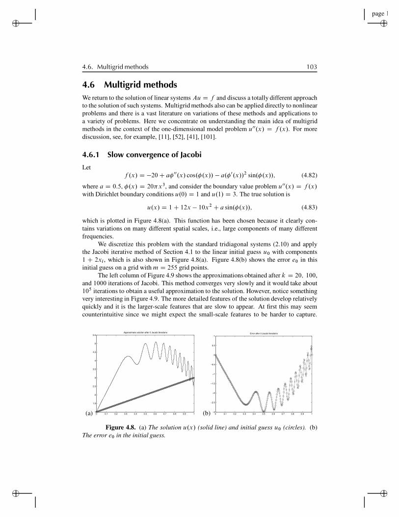
“rjlfdm”2007/6/1page 103✐
✐✐
✐
✐✐
✐✐
4.6. Multigrid methods 103
4.6 Multigrid methodsWe return to the solution of linear systems Au D f and discuss a totally different approachto the solution of such systems. Multigrid methods also can be applied directly to nonlinearproblems and there is a vast literature on variations of these methods and applications toa variety of problems. Here we concentrate on understanding the main idea of multigridmethods in the context of the one-dimensional model problem u00.x/ D f .x/. For morediscussion, see, for example, [11], [52], [41], [101].
4.6.1 Slow convergence of JacobiLet
f .x/ D !20 C a!00.x/ cos.!.x// ! a.!0.x//2 sin.!.x//; (4.82)
where a D 0:5, !.x/ D 20"x3, and consider the boundary value problem u00.x/ D f .x/with Dirichlet boundary conditions u.0/ D 1 and u.1/ D 3. The true solution is
u.x/ D 1 C 12x ! 10x2 C a sin.!.x//; (4.83)
which is plotted in Figure 4.8(a). This function has been chosen because it clearly con-tains variations on many different spatial scales, i.e., large components of many differentfrequencies.
We discretize this problem with the standard tridiagonal systems (2.10) and applythe Jacobi iterative method of Section 4.1 to the linear initial guess u0 with components1 C 2xi , which is also shown in Figure 4.8(a). Figure 4.8(b) shows the error e0 in thisinitial guess on a grid with m D 255 grid points.
The left column of Figure 4.9 shows the approximations obtained after k D 20; 100,and 1000 iterations of Jacobi. This method converges very slowly and it would take about105 iterations to obtain a useful approximation to the solution. However, notice somethingvery interesting in Figure 4.9. The more detailed features of the solution develop relativelyquickly and it is the larger-scale features that are slow to appear. At first this may seemcounterintuitive since we might expect the small-scale features to be harder to capture.
(a) 0 0.1 0.2 0.3 0.4 0.5 0.6 0.7 0.8 0.9 11
1.5
2
2.5
3
3.5
4
4.5
5
5.5Approximate solution after 0 Jacobi iterations
(b) 0 0.1 0.2 0.3 0.4 0.5 0.6 0.7 0.8 0.9 1−3
−2.5
−2
−1.5
−1
−0.5
0
0.5
1Error after 0 Jacobi iterations
Figure 4.8. (a) The solution u.x/ (solid line) and initial guess u0 (circles). (b)The error e0 in the initial guess.
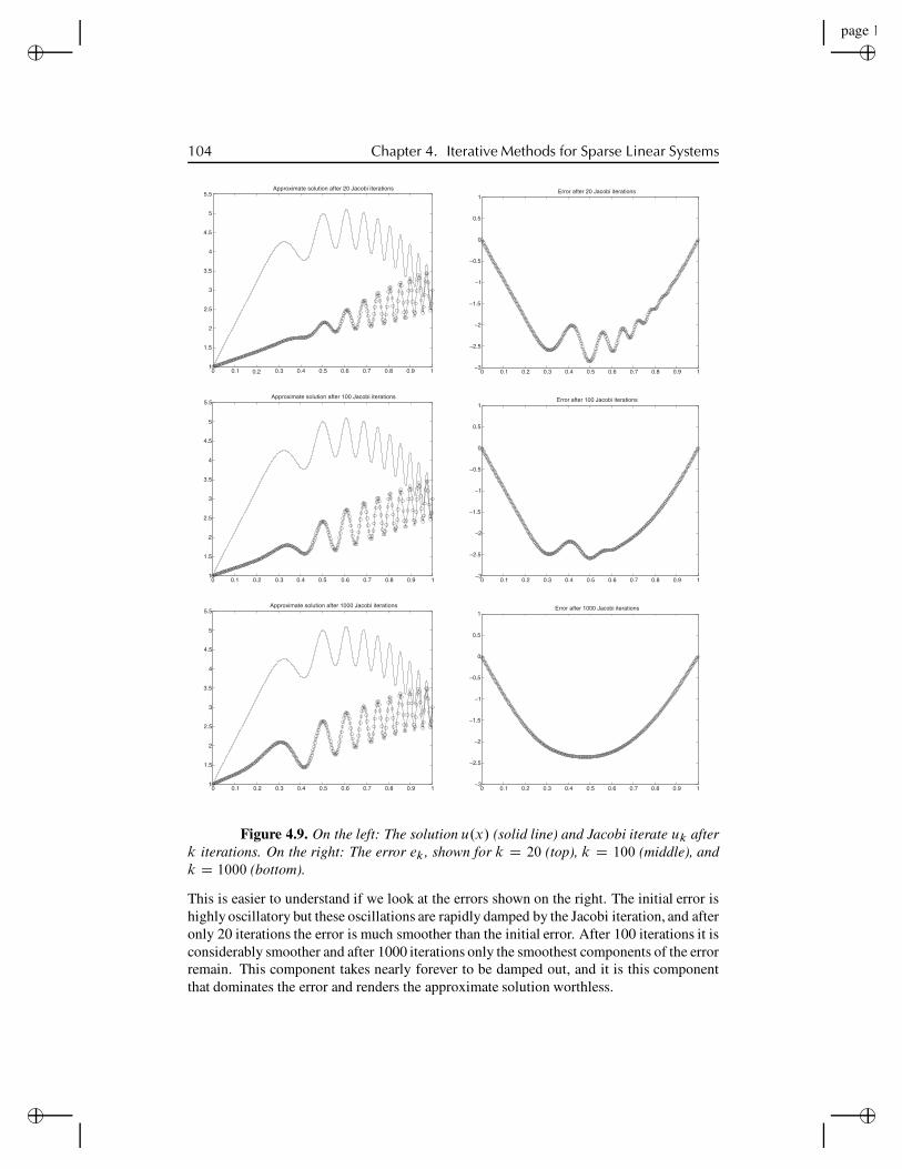
“rjlfdm”2007/6/1page 104✐
✐✐
✐
✐✐
✐✐
104 Chapter 4. Iterative Methods for Sparse Linear Systems
0 0.1 0.2 0.3 0.4 0.5 0.6 0.7 0.8 0.9 11
1.5
2
2.5
3
3.5
4
4.5
5
5.5Approximate solution after 20 Jacobi iterations
0 0.1 0.2 0.3 0.4 0.5 0.6 0.7 0.8 0.9 1−3
−2.5
−2
−1.5
−1
−0.5
0
0.5
1Error after 20 Jacobi iterations
0 0.1 0.2 0.3 0.4 0.5 0.6 0.7 0.8 0.9 11
1.5
2
2.5
3
3.5
4
4.5
5
5.5Approximate solution after 100 Jacobi iterations
0 0.1 0.2 0.3 0.4 0.5 0.6 0.7 0.8 0.9 1−3
−2.5
−2
−1.5
−1
−0.5
0
0.5
1Error after 100 Jacobi iterations
0 0.1 0.2 0.3 0.4 0.5 0.6 0.7 0.8 0.9 11
1.5
2
2.5
3
3.5
4
4.5
5
5.5Approximate solution after 1000 Jacobi iterations
0 0.1 0.2 0.3 0.4 0.5 0.6 0.7 0.8 0.9 1−3
−2.5
−2
−1.5
−1
−0.5
0
0.5
1Error after 1000 Jacobi iterations
Figure 4.9. On the left: The solution u.x/ (solid line) and Jacobi iterate uk afterk iterations. On the right: The error ek , shown for k D 20 (top), k D 100 (middle), andk D 1000 (bottom).
This is easier to understand if we look at the errors shown on the right. The initial error ishighly oscillatory but these oscillations are rapidly damped by the Jacobi iteration, and afteronly 20 iterations the error is much smoother than the initial error. After 100 iterations it isconsiderably smoother and after 1000 iterations only the smoothest components of the errorremain. This component takes nearly forever to be damped out, and it is this componentthat dominates the error and renders the approximate solution worthless.
“rjlfdm”2007/6/1page 105✐
✐✐
✐
✐✐
✐✐
4.6. Multigrid methods 105
To understand why higher frequency components of the error are damped most rapidly,recall from Section 4.2 that the error ek D uk D u! satisfies
ek D Gek"1;
where, for the tridiagonal matrix A,
G D I C h2
2A D
2
66666664
0 1=21=2 0 1=2
1=2 0 1=2: : :
: : :: : :
1=2 0 1=21=2 0
3
77777775
:
The i th element of ek is simply obtained by averaging the .i ! 1/ and .i C 1/ elements ofek"1 and this averaging damps out higher frequencies more rapidly than low frequencies.This can be quantified by recalling from Section 4.1 that the eigenvectors of G are the sameas the eigenvectors of A. The eigenvector up has components
upj D sin.!pxj / .xj D j h; j D 1; 2; : : : ; m/; (4.84)
while the corresponding eigenvalue is
"p D cos.p!h/ (4.85)
for p D 1; 2; : : : ; m. If we decompose the initial error e0 into eigencomponents,
e0 D c1u1 C c2u2 C " " "C cmum; (4.86)
then we haveek D c1"
k1 u1 C c2"
k2 u2 C " " "C cm"
kmum: (4.87)
Hence the pth eigencomponent decays at the rate " kp as k increases. For large k the error
is dominated by the components c1"k1 u1 and cm"
kmum, since these eigenvalues are closest
to 1:
"1 D !"m # 1 ! 1
2!2h2:
This determines the overall convergence rate, as discussed in Section 4.1.Other components of the error, however, decay much more rapidly. In fact, for half
the eigenvectors, those with m=4 $ p $ 3m=4, the eigenvalue "p satisfies
j"pj $ 1p2# 0:7
and j"pj20 < 10"3, so that 20 iterations are sufficient to reduce these components of theerror by a factor of 1000. Decomposing the error e0 as in (4.86) gives a Fourier sine seriesrepresentation of the error, since up in (4.84) is simply a discretized version of the sine
“rjlfdm”2007/6/1page 106✐
✐✐
✐
✐✐
✐✐
106 Chapter 4. Iterative Methods for Sparse Linear Systems
function with frequency p. Hence eigencomponents cpup for larger p represent higher-frequency components of the initial error e0, and so we see that higher-frequency compo-nents decay more rapidly.
Actually it is the middle range of frequencies, those nearest p ! m=2, that decaymost rapidly. The highest frequencies p ! m decay just as slowly as the lowest frequenciesp ! 1. The error e0 shown in Figure 4.9 has a negligible component of these highestfrequencies, however, and we are observing the rapid decay of the intermediate frequenciesin this figure.
For this reason Jacobi is not the best method to use in the context of multigrid. Abetter choice is underrelaxed Jacobi, where
ukC1 D .1 " !/uk C !Guk (4.88)
with ! D 2=3. The iteration matrix for this method is
G! D .1 " !/I C !G (4.89)
with eigenvalues!p D .1 " !/C ! cos.p"h/: (4.90)
The choice ! D 2=3 minimizes maxm=2<p!m j!pj, giving optimal smoothing of highfrequencies. With this choice of !, all frequencies above the midpoint p D m=2 havej!pj # 1=3.
As a standalone iterative method this would be even worse than Jacobi, since low-frequency components of the error decay even more slowly (!1 is now 1
3 C 23 cos."h/ !
1 " 13"
2h2), but in the context of multigrid this does not concern us. What is important isthat the upper half of the range frequencies are all damped by a factor of at least 1=3 periteration, giving a reduction by a factor of .1=3/3 ! 0:037 after only three iterations, forexample.
4.6.2 The multigrid approachWe are finally ready to introduce the multigrid algorithm. If we use underrelaxed Jacobi,then after only three iterations the high-frequency components of the error have alreadydecayed significantly, but convergence starts to slow down because of the lower-frequencycomponents. But because the error is now much smoother, we can represent the remainingpart of the problem on a coarser grid. The key idea in multigrid is to switch now to a coarsergrid to estimate the remaining error. This has two advantages. Iterating on a coarser gridtakes less work than iterating further on the original grid. This is nice but is a relativelyminor advantage. Much more important, the convergence rate for some components of theerror is greatly improved by transferring the error to a coarser grid.
For example, consider the eigencomponent p D m=4 that is not damped so much byunderrelaxed Jacobi, !m=4 ! 0:8, and after three iterations on this grid this component ofthe error is damped only by a factor .0:8/3 D 0:512. The value p D m=4 is not in theupper half of frequencies that can be represented on a grid with m points—it is right in themiddle of the lower half.
However, if we transfer this function to a grid with only half as many points, itis suddenly at the halfway point of the frequencies we can represent on the coarser grid

“rjlfdm”2007/6/1page 107✐
✐✐
✐
✐✐
✐✐
4.6. Multigrid methods 107
(p ! mc=2 now, where mc D .m " 1/=2 is the number of grid points on the coarser grid).Hence this same component of the error is damped by a factor of .1=3/3 ! 0:037 afteronly three iterations on this coarser grid. This is the essential feature of multigrid.
But how do we transfer the remaining part of the problem to a coarser grid? We don’ttry to solve the original problem on a coarser grid. Instead we solve an equation for theerror. Suppose we have taken ! iterations on the original grid and now want to estimatethe error e! D u! " u!. This is related to the residual vector r! D f " Au! by the linearsystem
Ae! D "r! : (4.91)
If we can solve this equation for e! , then we can subtract e! from u! to obtain the desiredsolution u!. The system (4.91) is the one we approximate on a coarsened grid. After takinga few iterations of Jacobi on the original problem, we know that e! is smoother than thesolution u to the original problem, and so it makes sense that we can approximate thisproblem well on a coarser grid and then interpolate back to the original grid to obtain thedesired approximation to e! . As noted above, iterating on the coarsened version of thisproblem leads to much more rapid decay of some components of the error.
The basic multigrid algorithm can be informally described as follows:
1. Take a fixed number of iterations (e.g., ! D 3) of a simple iterative method (e.g.,underrelaxed Jacobi or another choice of “smoother”) on the original m # m systemAu D f . This gives an approximation u! 2 Rm.
2. Compute the residual r! D f " Au! 2 Rm.
3. Coarsen the residual: approximate the grid function r! on a grid with mc D .m"1/=2points to obtain Qr 2 Rmc .
4. Approximately solve the system QA Qe D "Qr , where QA is the mc # mc version of A(the tridiagonal approximation to d2=dx2 on a grid with mc points).
5. The vector Qe approximates the error in u! but only at mc points on the coarse grid.Interpolate this grid function back to the original grid with m points to obtain anapproximation to e!. Subtract this from u! to get a better approximation to u!.
6. Using this as a starting guess, take a few more iterations (e.g., ! D 3) of a simpleiterative method (e.g., underrelaxed Jacobi) on the original m # m system Au D fto smooth out errors introduced by this interpolation procedure.
The real power of multigrid comes from recursively applying this idea. In step 4of the algorithm above we must approximately solve the linear system QA Qe D "Qr of sizemc . As noted, some components of the error that decayed slowly when iterating on theoriginal system will now decay quickly. However, if mc is still quite large, then there willbe other lower-frequency components of the error that still decay abysmally slowly on thiscoarsened grid. The key is to recurse. We only iterate a few times on this problem beforeresorting to a coarser grid with .mc " 1/=2 grid points to speed up the solution to thisproblem. In other words, the entire algorithm given above is applied within step 4 to solvethe linear system QA Qe D "Qr . In a recursive programming language (such as MATLAB) thisis not hard to implement and allows one to recurse back as far as possible. If m C 1 is a

“rjlfdm”2007/6/1page 108✐
✐✐
✐
✐✐
✐✐
108 Chapter 4. Iterative Methods for Sparse Linear Systems
(a) 0 0.2 0.4 0.6 0.8 11
1.5
2
2.5
3
3.5
4
4.5
5
5.5Level 7 After 1 Vcycles
(b) 0 0.2 0.4 0.6 0.8 10.12
0.1
0.08
0.06
0.04
0.02
0
0.02|| Error || = 0.11806
Figure 4.10. (a) The solution u.x/ (solid line) and approximate solution (circles)obtained after one V-cycle of the multigrid algorithm with ! D 3. (b) The error in thisapproximation. Note the change in scale from Figure 4.9(b).
power of 2, then in principle one could recurse all the way back to a coarse grid with onlya single grid point, but in practice the recursion is generally stopped once the problem issmall enough that an iterative method converges very quickly or a direct method such asGaussian elimination is easily applied.
Figure 4.10 shows the results obtained when the above algorithm is used starting withm D 28 ! 1 D 255, using ! D 3, and recursing down to a grid with three grid points, i.e.,seven levels of grids. On each level we apply three iterations of underrelaxed Jacobi, do acoarse grid correction, and then apply three more iterations of under-relaxed Jacobi. Hencea total of six Jacobi iterations are used on each grid, and this is done on grids with 2j ! 1points for j D 8; 7; 6; 5; 4; 3; 2, since the coarse grid correction at each level requiresdoing this recursively at coarser levels. A total of 42 underrelaxed Jacobi iterations areperformed, but most of these are on relatively coarse grids. The total number of grid valuesthat must be updated in the course of these iterations is
6
8X
jD2
2j " 6 # 29 D 3072;
roughly the same amount of work as 12 iterations on the original grid would require. Butthe improvement in accuracy is dramatic—compare Figure 4.10 to the results in Figure 4.9obtained by simply iterating on the original grid with Jacobi.
More generally, suppose we start on a grid with m C 1 D 2J points and recurse allthe way down, taking ! iterations of Jacobi both before and after the coarse grid correctionon each level. Then the work is proportional to the total number of grid values updated,which is
2!
JX
jD2
2j " 4!2J " 4!m D O.m/: (4.92)
Note that this is linear in the number of grid points m, although as m increases we are usingan increasing number of coarser grids. The number of grids grows at the rate of log2.m/but the work on each grid is half as much as the previous finer grid and, so the total work

“rjlfdm”2007/6/1page 109✐
✐✐
✐
✐✐
✐✐
4.6. Multigrid methods 109
is O.m/. This is the work required for one “V-cycle” of the multigrid algorithm, startingon the finest grid, recursing down to the coarsest grid and then back up as illustrated inFigure 4.11(a) and (b). Taking a single V-cycle often results in a significant reduction inthe error, as illustrated in Figure 4.10, but more than one V-cycle might be required toobtain a sufficiently accurate solution. In fact, it can be shown that for this model problemO.log.m// V-cycles would be needed to reach a given level of error, so that the total workwould grow like O.m log m/.
We might also consider taking more that one iteration of the cycle on each of thecoarser grids to solve the coarse grid problems within each cycle on the finest grid. Sup-pose, for example, that we take two cycles at each stage on each of the finer grids. Thisgives the W-cycle illustrated in Figure 4.11(c).
Even better results are typically obtained by using the “full multigrid” (FMG) algo-rithm, which consists of starting the process on the coarsest grid level instead of the finestgrid. The original problem u00.x/ D f .x/ is discretized and solved on the coarsest levelfirst, using a direct solver or a few iterations of some iterative method. This approximationto u.x/ is then interpolated to the next finer grid to obtain a good initial guess for solvingthe problem on this grid. The two-level multigrid algorithm is used on this level to solvethe problem. The result is then interpolated to the next-level grid to give good initial datathere, and so on. By the time we get to the finest grid (our original grid, where we want thesolution), we have a very good initial guess to start the multigrid process described above.This process is illustrated using the V-cycle in Figure 4.12.
This start-up phase of the computation adds relatively little work since it is mostlyiterating on coarser grids. The total work for FMG with one V-cycle is only about 50%more than for the V-cycle alone. With this initialization process it often turns out that oneV-cycle then suffices to obtain good accuracy, regardless of the number of grid points. In
h-grid
2h-grid
4h-grid
(a) (b) (c)
Figure 4.11. (a) One V-cycle with two levels. (b) One V-cycle with three levels.(c) One W-cycle with three levels.
h-grid
2h-grid
4h-grid
Figure 4.12. FMG with one V-cycle on three levels.
“rjlfdm”2007/6/1page 110✐
✐✐
✐
✐✐
✐✐
110 Chapter 4. Iterative Methods for Sparse Linear Systems
this case the total work is O.m/, which is optimal. For the example shown in Figure 4.10,switching to FMG gives an error of magnitude 6 ! 10!3 after a single V-cycle.
Of course in one dimension simply solving the tridiagonal system requires onlyO.m/ work and is easier to implement, so this is not so impressive. But the same re-sult carries over to more space dimensions. The FMG algorithm for the Poisson problemon an m ! m grid in two dimensions requires O.m2/ work, which is again optimal sincethere are this many unknowns to determine. Recall that fast Poisson solvers based on theFFT require O.m2 log m/ work, while the best possible direct method would require .m3/.Applying multigrid to more complicated problems can be more difficult, but optimal resultsof this sort have been achieved for a wide variety of problems.
The multigrid method described here is intimately linked to the finite difference gridbeing used and the natural manner in which a vector and matrix can be “coarsened” bydiscretizing the same differential operator on a coarser grid. However, the ideas of multigridcan also be applied to other sparse matrix problems arising from diverse applications whereit may not be at all clear how to coarsen the problem. This more general approach is calledalgebraic multigrid (AMG); see, for example, [76], [86].


