Published inInt. J. of Solids and Structures

161 (2019), 219–227

Finite difference model of wave motion for Structural

Health Monitoring of Single Lap Joints

Stefano Carrino, Francesco Nicassio, Gennaro Scarselli

Department of Innovation Engineering, University of Salento, Lecce, Italy

Raffaele Vitolo

Department of Mathematics and Physics “E. De Giorgi”, University of Salento, Lecce,Italy

Abstract

This study is focused on the development of a finite difference model tosimulate Lamb wave propagation through Single Lap Joints (SLJs). Themain advantage of this model is the mathematical ability to easily reproducethe presence of a damage (debonding) as a discontinuity in velocity values.This makes our model suitable for continuous and embedded StructuralHealth Monitoring (SHM) of a complex structure. Numerical simulationsand experimental campaigns are presented in order to validate the proposedmodel.

Keywords: Finite difference model, Lamb waves, structural healthmonitoring, single lap joints.

1. Introduction

Adhesive joints are used in aerospace, automotive and marine industriesfor their good mechanical properties and light weight. For several structuralapplications, they represent the only feasible method of joining componentswith advantages in terms of cost, optimal stress distribution and ease of

Email addresses: stefano.carrino@unisalento.it,

francesco.nicassio@unisalento.it, gennari.scarselli@unisalento.it (StefanoCarrino, Francesco Nicassio, Gennaro Scarselli), raffaele.vitolo@unisalento.it(Raffaele Vitolo)

manufacturing. Bonded joints distribute forces over a large area avoidingstress peaks that could arise by using fasteners like bolts, rivets or screws.

Despite these positive aspects, bonded joints are subject to fatigue degra-dation of the adhesive layer, disbonds and voids due to non-accurate man-ufacturing processes that reduce the load carrying capability, leading tofailure as studied in [11].

For the above reasons, the development of SHM systems is necessary inorder to ensure reliability and safety of adhesively bonded joints in complexstructures. SHM also contributes to a better knowledge of the mechanicalproperties of the structures [31]. Over the past decades, several studies havebeen carried out on investigating the dynamic response of the adhesive jointsand the development of efficient Non-Destructive Techniques (NDT) in or-der to detect, evaluate and localise defects or damages eventually presentin bonded areas.

Conventional NDT are of limited use because they require to put outof service the structure for a non-negligible time period in order to executepost-damage inspections. In addition to the Visual Testing (VT), which isby far the most common non-destructive examination, Ultrasonic A- andC-scan, X-ray and thermography can be employed to inspect structuralcomponents. In ultrasonic scanning, a transducer generates pulses of shearor compression waves at frequency of 1 to 20 MHz that, during the propaga-tion through the adhesion zone, is modified by the path taken and a part ofenergy is reflected by discontinuities. A- and C-scan consist in the evalua-tion of the magnitude of the reflected echoes thus obtaining a map of defectsby scanning the surface of a structure. In [27] a non-destructive testing ofthe lower and upper wing skins was performed by use of an A- and C-scantransducer obtaining information regarding the condition of composites andthe integrity of the composite-to-titanium bonded joint. A large defect wasfound in a lower wing skin outlining the boundary and the location of defectthrough the thickness.

X-ray techniques, in contrast to ultrasound and thermography, can pro-vide a 3D image of a damage. In [21] a methodology to evaluate the through-thickness distribution of damage in a [(0o/90o)2]S Carbon Fibre ReinforcedPlastic (CFRP) panels subjected to low velocity impact is developed: de-laminations were mapped by a 3D ply-by-ply damage visualisation.

An Infrared (IR) NDT of interlaminar disbonds on fibre metal lami-nate hybrid composites was proposed in [26]: a point-wise laser heat source(Flying Laser Spot Thermography) was moved along a raster scanning tra-

2

jectory over the structure surface; an IR camera was employed to acquirethe temperature field induced by the moving heat source; disbonds and de-fects were then detected by analysing the perturbations of the temperaturedistribution.

Yashiro et al. in [36] evaluated fatigue-induced disbond in CFRP double-lap joints using embedded Fibre Bragg Grating (FBG) sensors. The studyis based on a change in the spectrum shapes of FBG sensors embeddednear the bond-line. These sensors experienced a step-like strain distribu-tion due to the intact load-carrying section and the disbonded stress-freesection. The disbond area was determined from the evaluation of the re-flection spectrum of FBG sensors embedded in different lines of a joint.

In [24] adhesively bonded CFRP samples were investigated by usingElectroMechanical Impedance (EMI) technique. This is based on directand converse effects of piezoelectric sensor (PZT) attached on the inspectedstructure. The electrical response picked up on the sensor is related tomechanical characteristics of the structure and then to the modification ofadhesive bonds. Various techniques are based on nonlinear acoustics meth-ods: the Contact Acoustic Nonlinearity (CAN) ([34], [6]), vibro-acousticswave modulation, nonlinear elastic wave spectroscopy and the Local DefectResonance (LDR) ([33], [8]). LDR is based on the local rigidity decrease ofa certain mass associated with the defect area which causes the arising of aspecific frequency related to the characteristic of the defect. In [8] the useof nonlinear waves for detection of disbonds in adhesive joints was investi-gated. Subharmonics, nonlinear intermodulation of the driving frequencyand defect resonance frequencies were correlated to the interaction betweenthe used elastic waves and disbonded regions.

One of the most promising techniques that enables inspections at longdistances is based on the application of Ultrasonic Guided Waves (UGWs)[9, 19] such as acousto-ultrasonic induced Lamb waves. This techniqueconsists in exciting Lamb waves by a piezoelectric transducer attached to thestructure’s surface which can be detected by a network of multiple sensors.The presence of defects or damages in the investigated domain alters thesignal propagation, resulting in a received signal which is different from theone that was initially generated.

Non-linear ultrasonic waves are used also in [30] for assessment of debond-ing in SLJ: the presence of microbubbles in the bond due to the manufactur-ing process was investigated by interpretating the experimental behavioursand tomographic tests. In [32] the phase and the amplitude of the structural

3

SLJ response excited by an harmonic excitation was evaluated in order tocharacterise defects and damages within the adhesive region according tothe dynamic response. In [25] an experimental investigation of the use ofLamb waves for the monitoring of stiffened metallic structures was carriedout: the size and shape of defect was evaluated and visualised by a win-dowed root-mean-squared technique for quantifying of reflected, attenuatedand transmitted energy. A baseline-free technique is proposed in [28] whichis based on the detection of modes generated by disbonds. It was demon-strated that the disbond caused reflection, refraction and mode conversionof the incident S0 wave. Several sensors distributed parallel to the edge ofbonded area allow the identification of disbonds by the appearance of wavemodes.

Jankauskas and Mazeika in [13] carried out a numerical and experimentalstudy of zero-mode Lamb waves propagation through a lap joint weldedplates used in storage tank floors. It was demonstrated that the transmissionlosses of the S0 mode vary depending on the ratio between lap joint widthand wavelength providing information for the defect or damage geometrydefinition. A mode similar to S0 Lamb wave propagation was used in [7]that can be used for inspection of large welded plate so to detect defects suchas cracking or corrosion along the length of weld. Huthwaite in [12] usedguided wave tomography to produce thickness maps of corrosion damageand defects by sending guided waves through the studied region.

In [3] fundamental Lamb wave modes was characterised in terms of prop-agation parameters through Finite Element Method (FEM) in commercialsoftware in order to study the wave behaviour on a plate between two solidbodies with imperfect contact conditions. Ren and Lissenden in [29] carriedout a fully coupled multi-physics finite element analysis, which includes thedriving circuit and the piezoelectric elements, in order to study the excita-tion of circular crested waves due to PZT discs for different sensor geome-try and adhesive thickness. In [15] a semi-analytical finite element (SAFE)method wad used to model the distributed electrical excitation and scat-tering of the waves at discontinuities by using piezoelectric elements. TheLamb waves were modelled by Spectral Element Method (SEM) as in [23]and [20]. Liu et al. in [22] presented a two-layer spectral finite elementmodel to simulate PZT-induced Lamb wave propagation in beam-like andplate-like structures where the dynamic equation was derived from Hamil-ton’s principle.

A Finite Difference Method (FDM) was used in ([35], [2], [14]) to simu-

4

late multiple modes of Lamb waves in aluminium SLJ generated by using anexcitation toneburst representing the PZTs action. In [35] an explicit FiniteDifference (FD) scheme was applied to solve propagating Lamb waves. Bal-asubramanyam in [2] describes a FDM to simulate S0 and A0 in plane metalsheets obtaining the time-domain histories of displacement field. In [14] theexcitation and propagation of Lamb waves by inter-digital transducer wasmodelled analytically and then compared to experimental measure obtainedby exciting Lamb waves in an aluminium plate.

For the sake of completeness, the papers [5, 16, 17, 18] shall be men-tioned. Here, nonlinear wave equations of KdV, Boussinesq or other typeswere considered as mathematical models. It was proved, both mathemati-cally and experimentally, that solitons traveling in a delaminated materialare subject to fission, hencey they are suitable to detecting defects. Thistechnique, however, has a higher level of experimental complexity involvingthe use of laser and optical equipment, also if it might be more suitable thanthe technique presented in this paper in the case of long elastic waveguides.

Although the techniques mentioned are suitable to assess the health ofbonded areas, only UGWs allow the continuous and embedded time moni-toring of the structures.

In this work a numerical and experimental investigation of Single LapJoints (SLJs) structural health by using Lamb waves propagation is pre-sented. The aim was to monitor the state of adhesive region and estimatethe size of possible disbonds.

The paper is divided in two part: the mathematical model and its nu-merical implementation, and the experimental part.

The mathematical model stems from the Cauchy–Navier equation forelastodynamics [10]. The key feature lies in the fact that the space-dependentLame coefficients have discontinuity on the boundary with the debonded re-gion. The discretisation of this equation has to be performed by keepinginto account that the derivatives of the Lame coefficients will contribute tothe FDM.

Experiments on the propagation of S0 through the adhesive zone wereperformed by using two PZT sensors attached on the upper and lower platein pitch&catch configuration. The S0 mode was used to investigate the in-tegrity of adhesive in bonded zone. Frequencies below the cut-off value wereused in order to avoid the presence of higher symmetric and antisymmetricmodes. The received signals were transformed by Fast Fourier Transform(FFT) in order to correlate frequency spectra to the structural health of

5

adhesive. Several wave packets with different driving frequencies were usedto investigate the bonded area. Experiments revealed, in agreement withnumerical simulations, that for each disbond length there is a given drivingfrequency at which the wave packet is attenuated and presents a deformedshape of frequency spectrum.

In this way, for SLJ structure, a novel reduced-order FD model is ob-tained and it appears leaner, cleaner and more simplified than FE model.The fact that numerical simulations were carried out by a relatively simpleMatlab code with a short execution time represents one point of strengthof the proposed approach, also in view of industrial applications.

2. The model

We make use of Cauchy–Navier’s equation for elastodynamics [10]:

ρutt = µ∆u + (λ+ µ)∇(div u) + 2∇u∇µ+ (div u)∇λ+ ρf (1)

where u is the displacement vector field, λ and µ are the Lame coefficients(that in our case depend on the spatial point), ρ is the (space-dependent)density and f is the force per unit mass. We also recall that

∇u =1

2(∇u +∇uT ) (2)

We use the above equations as a model for a horizontal plate where elas-tic waves propagate in the x and z direction. The displacement of particlesoccur both in the direction of propagation and along the thickness of theplate (y-direction). If the domain of equation (1) is a plane perpendicular tothe z axis, passing through the application point of f , there is no displace-ment in the third direction z, hence our problem becomes 2-dimensional.

Let us introduce the notation u = (u(x, y), v(x, y)) for the displacementsin the x, y directions, respectively, and the notation f = (fx(x, y), fy(x, y))for the force per unit mass. Then the system (1) becomes

ρutt =µ(uxx + uyy) + (λ+ µ)(uxx + vxy)+ (3a)

(2uxµx + (uy + vx)µy) + (ux + vy)λx + ρfx (3b)

ρvtt =µ(vxx + vyy) + (λ+ µ)(uxy + vyy)+ (3c)

((uy + vx)µx + 2vyµy) + (ux + vy)λy + ρfy (3d)

6

Provided we neglect terms multiplied by ρx or ρy (they give a small contri-bution in our physical situation), we can recast the above equations in thefollowing form:(

λ+ 2µ

ρux +

λ

ρvy

)x

+

(µ

ρ(uy + vx)

)y

+ fx = utt (4a)(µ

ρ(uy + vx)

)x

+

(λ

ρux +

λ+ 2µ

ρvy

)y

+ fy = vtt (4b)

We add to the above model stress-free boundary conditions on the upperand the lower surfaces of the plate:

λ

ρux +

λ+ 2µ

ρvy = 0 (5a)

µ

ρ(uy + vx) = 0 (5b)

Usually, the above equations are expressed through the longitudinal wavespeed cL and the shear wave speed cT :

c2L =λ+ 2µ

ρ, c2T =

µ

ρ, (6)

and we have(c2Lux + (c2L − 2c2T )vy

)x

+(c2T (uy + vx)

)y

+ fx = utt (7a)(c2T (uy + vx)

)x

+((c2L − 2c2T )ux + c2Lvy

)y

+ fy = vtt (7b)

with boundary conditions

(c2L − 2c2T )ux + c2Lvy = 0 (8a)

c2T (uy + vx) = 0 (8b)

3. Finite difference method

We model the domain of the unknown functions u, v as Ix × Iy × It,where

Ix = [0, lx], Iy = [0, ly], It = [0, lt], (9)

7

with lx, ly and lt positive constants. The space and time grid of the problemis constructed by an equal increment ∆x = ∆y in the x and y directions,and a time interval ∆t. Following [1], we require that

∆t ≤ ∆x√c2L + c2T

(10)

for stability. This amounts at requiring that the signals will not propagateacross one grid rectangle in a time that is shorter than one time interval.We assume that the numbers Nx = lx/∆x and Ny = ly/∆y are integer,possibly by redefining the intervals to the nearest values lx or ly. We willindex points (xi, yj) with 1 ≤ i ≤ Nx + 2, 1 ≤ j ≤ Ny + 2, where

x1 = −∆x xNx+2 = lx + ∆x (11)

y1 = −∆y yNy+2 = ly + ∆y (12)

so that the nodes x1, y1, xNx+2, yNy+2 are indeed pseudo-nodes (they lieoutside the domain, see Figure 1). Finally, we suppose that Nt = lt/∆t isan integer.

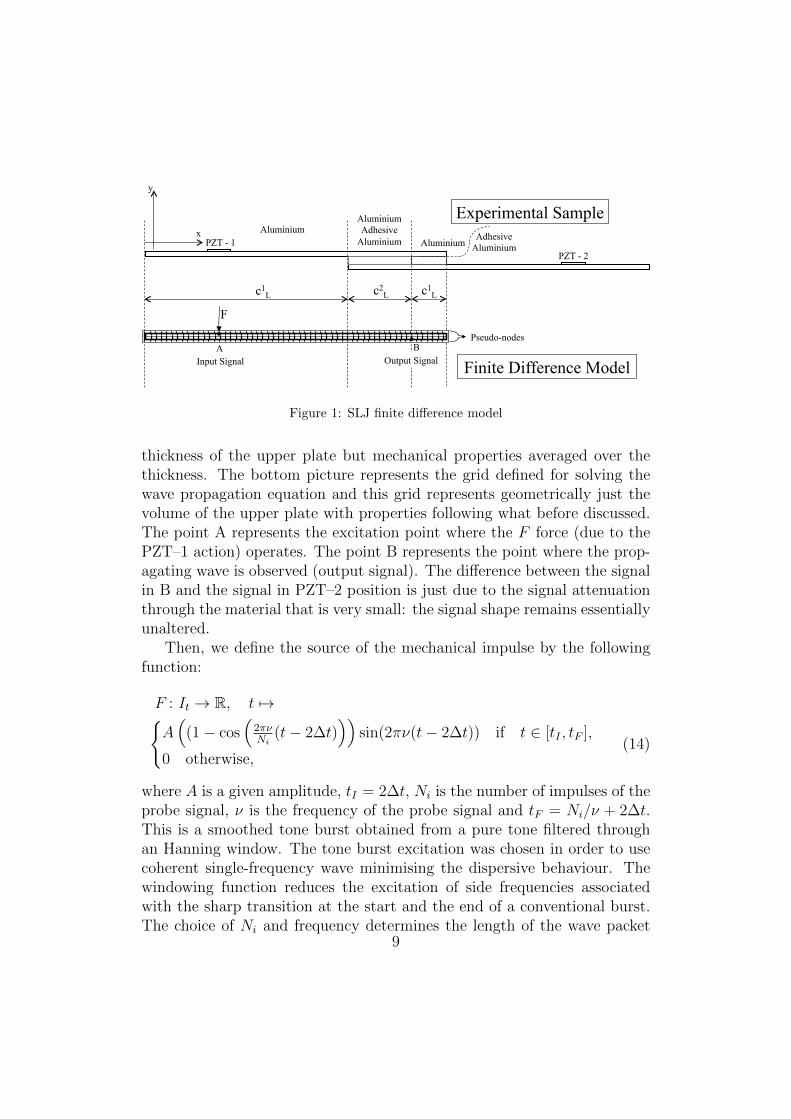
The functions cL, cT and ρ are functions of (x, y), and they are non-constant as their values change in the spatial points where the bonding isno longer homogeneous. In this work, we suppose that the non-homogeneityof the bonding holds along the x direction only. In particular, we assumethat there is an interval [xI , xF ] ⊂ Ix where the bonding is loose. We definethe function cL on the grid according with the above model as follows:

cL(i, j) =

{c1L if xi 6∈ [xI , xF ],

c2L if xi ∈ [xI , xF ],(13)

where c1L and c2L are two constants. We make a similar definition for cTand ρ. In the Figure 1 the top picture represents a geometric section of theSLJ sample used for the experiments: it is possible to identify the positionof the two sensors, PZT–1 exciting the structure and PZT–2 receiving thesignal. In addition, it is possible to identify the two zones of the upper plateforming the joint, 1 and 2, in which the wave travels at different speeds, c1Land c2L. The zone 1 is affected only by the aluminum properties and theLamb waves propagate like in a 1.2 mm thick aluminum panel. The zone 2is characterised by the influence of the aluminum–adhesive–aluminum layerand c2L depends on the global joint thickness and on the mechanical prop-erties of aluminum and adhesive. Having this in mind, the zone 2 has the

8

Aluminium Adhesive

Aluminium Adhesive Aluminium

Aluminium PZT - 1

PZT - 2

F

Output Signal Finite Difference Model

x

y

A B

Aluminium

Experimental Sample

c1L

c2L

c1L

Input Signal

Pseudo-nodes

Figure 1: SLJ finite difference model

thickness of the upper plate but mechanical properties averaged over thethickness. The bottom picture represents the grid defined for solving thewave propagation equation and this grid represents geometrically just thevolume of the upper plate with properties following what before discussed.The point A represents the excitation point where the F force (due to thePZT–1 action) operates. The point B represents the point where the prop-agating wave is observed (output signal). The difference between the signalin B and the signal in PZT–2 position is just due to the signal attenuationthrough the material that is very small: the signal shape remains essentiallyunaltered.

Then, we define the source of the mechanical impulse by the followingfunction:

F : It → R, t 7→{A(

(1− cos(

2πνNi

(t− 2∆t)))

sin(2πν(t− 2∆t)) if t ∈ [tI , tF ],

0 otherwise,(14)

where A is a given amplitude, tI = 2∆t, Ni is the number of impulses of theprobe signal, ν is the frequency of the probe signal and tF = Ni/ν + 2∆t.This is a smoothed tone burst obtained from a pure tone filtered throughan Hanning window. The tone burst excitation was chosen in order to usecoherent single-frequency wave minimising the dispersive behaviour. Thewindowing function reduces the excitation of side frequencies associatedwith the sharp transition at the start and the end of a conventional burst.The choice of Ni and frequency determines the length of the wave packet

9

that has to be not too long in order to avoid the interference with thereflection due to the boundaries. Thus, bursts with less peaks are chosenfor the lower values of frequency used.

We should define the equations for the discrete unknowns u(i, j, k) andv(i, j, k), where i denotes the point xi, j stands for yj and k stands for tk.We proceed as follows: compute x and y derivatives in the equations (7),then replace the derivatives of the given and unknown functions with thefollowing discrete quantities:

ux(i, j, k) =1

2∆x(u(i+ 1, j, k)− u(i− 1, j, k)), (15a)

uy(i, j, k) =1

2∆y(u(i, j + 1, k)− u(i, j − 1, k)), (15b)

and analogously for v, and

(cL)x(i, j) =1

2∆x(cL(i+ 1, j)− cL(i− 1, j)), (15c)

(cL)y(i, j) =1

2∆y(cL(i, j + 1)− cL(i, j − 1)), (15d)

and analogously for cT , ρ, and

uxx(i, j, k) =1

∆x2(u(i+ 1, j, k)− 2u(i, j, k) + u(i− 1, j, k)), (15e)

uyy(i, j, k) =1

∆y2(u(i, j + 1, k)− 2u(i, j, k) + u(i, j − 1, k)), (15f)

uxy(i, j, k) =1

4∆x∆y(u(i+ 1, j + 1, k)− u(i− 1, j + 1, k)

− u(i+ 1, j − 1, k) + u(i− 1, j − 1, k)), (15g)

and analogously for v.We also need the discretisation of utt (and similarly the discretisation of

vtt):

utt(i, j, k) =1

(∆t)2(u(i, j, k + 1)− 2u(i, j, k) + u(i, j, k − 1)). (16)

Finally, we define

fx(i, j, k) =F (tk), for i = 2 (to bypass the pseudo-node x1), (17a)

fx(i, j, k) =0 otherwise, (17b)

fy(i, j, k) =0, (17c)

10

as we would like to simulate the production of waves on one side of theplate. As showed in the Figure 1, i = 2 corresponds to the edge of theplate, while i = 1 and i = Nx + 2 correspond to the pseudo-nodes used tosatisfy the Lamb wave boundary conditions (stress-free surface).

The boundary conditions are implemented by the following equations atthe edges of Ix (for inner values of yj):

u(1, j, k) =C∆x

2∆y(v(2, j + 1, k)− v(2, j − 1, k)) + u(2, j, k), (18a)

v(1, j, k) =∆x

2∆y(u(2, j + 1, k)− u(2, j − 1, k)) + v(2, j, k), (18b)

where C = (cL(2, j)2 − 2cT (2, j)2)/cL(2, j)2, and

u(Nx + 2, j, k) =− C ∆x

2∆y(v(Nx + 1, j + 1, k)− v(Nx + 1, j − 1, k))

+ u(Nx + 1, j, k); (19a)

v(Nx + 2, j, k) =− ∆x

2∆y(u(Nx + 1, j + 1, k)− u(Nx + 1, j − 1, k))

+ v(Nx + 1, j, k); (19b)

where C = (cL(Nx+1, j)2−2cT (Nx+1, j)2)/cL(Nx+1, j)2 and the followingequations at the edges of Iy (for inner values of xi):

u(i, 1, k) =∆y

2∆x(v(i+ 1, 2, k)− v(i− 1, 2, k)) + u(i, 2, k), (20a)

v(i, 1, k) =C∆y

2∆x(u(i+ 1, 2, k)− u(i− 1, 2, k)) + v(i, 2, k), (20b)

where C = (cL(i, 2)2 − 2cT (i, 2)2)/cL(i, 2)2, and

u(i, Ny + 2, k) =− ∆y

2∆x(v(i+ 1, Ny + 1, k)− v(i− 1, Ny + 1, k))

+ u(i, Ny + 1, k); (21a)

v(i, Ny + 2, k) =− C ∆y

2∆x(u(i+ 1, Ny + 1, k)− u(i− 1, Ny + 1, k))

+ v(i, Ny + 1, k); (21b)

where C = (cL(i, Ny + 1)2 − 2cT (i, Ny + 1)2)/cL(i, Ny + 1)2

11

In the system of equations (7) we can replace derivatives by the aboveapproximations, and get an evolutionary system of two algebraic equations(plus the boundary conditions). The system will be of the form

u(i, j, k + 1) =Fu(u(∗, ∗, k), v(∗, ∗, k), u(∗, ∗, k − 1), v(∗, ∗, k − 1)), (22a)

v(i, j, k + 1) =Fv(u(∗, ∗, k), v(∗, ∗, k), u(∗, ∗, k − 1), v(∗, ∗, k − 1)), (22b)

where Fu and Fv are two linear functions of the arguments, and the ‘*’ standfor the suitable space grid points, which allows to find the values of u andv on the space grid points (xi, yj) at the time tk+1 given all values of u andv on the space grid points (xi, yj) at the times tk, tk−1.

4. Experimental Set-up

The specimen adopted for the experimental campaign is a SLJ made oftwo aluminium plates (630 mm × 126 mm × 1.2 mm) with an overlap of 30mm (Figure 2). Here teflon film (length Deb) is applied in order to reduce

Signal Generator Amplifier

P1 P2

Oscilloscope

PC

deb

b th

Figure 2: Experimental set-up

the adhesive zone (length l) to simulate a disbond damage: six identicalsamples are manufactured, using increasing values of debonding (3 – 5 –7.5 – 10 – 12.5 – 15 mm). The proposed method works only for complete

12

debonding along the side b, with deb not varying along the b dimension. Inother terms, the approach is bidimensional. This limitation, indeed, doesnot affect the relevance of the approach: this 2D model, on one hand, isof practical interest for all the structural applications involving beamlikestructures (for which most of the debondings are expected to be of the kindherein treated); on the other hand, it represents the benchmark for a morecomplex extension to 3D models, where the geometries and the equationsare much more complicated than the ones reported in this paper.

During the experimental tests, stress-free conditions are achieved us-ing vibration-absorbing sponge under the free short edge and overlappedzone of the SLJ. In Figure 3 the overall experimental process is illustrated

Signal generation with νex

Signal amplification

P1 on sample

P2 on sample

Damage Deb Oscilloscope PC

Signal attenuation?

Y

N New νex

Figure 3: Schematic of the experimental set–up

while in Figure 2 the experimental set–up is presented (see also [4], whereother methods different from those presented in this work were discussed).The exciting input to the sample (tone burst with Ni peaks and exciting fre-quency νex) is provided by the signal generator TG5012A of Aim & ThurlbyThandar Instrument and powered (multiplying by 50 the input voltage) byFalco System WMA – 300, feeding the exciting piezo-sensor P1 with lowharmonic distortion – low phase noise – high frequency resolution; the signalexcites the overlap zone and comes into the receiver sensor P2, that is con-nected to the oscilloscope Serie 3000 PicoScope. With Single Trigger modecontrol, the scope monitors the incoming signal and waits for the voltageto rise above a given threshold (variable for each disbond length); then,it causes the scope to capture and display just the first received waveformon P2. All signals are low-pass filtered and processed using software Pico-Scope 6 and MATLAB codes on PC in order to detect the differences forthe various investigated disbond lengths. This real-time acquisition of thepropagating waveforms allows to monitor the output signal: νex must bechanged as long as the P2 signal does not contain changes, suggesting thepresence of damage in the overlap zone, in terms of waveform (Figure 4–leftgraphs) and frequency spectrum (Figure 4–right graphs, obtained by FFTof the transient acquired packets).

13

Amplitude

Time

Amplitude

Frequency

Figure 4: Output signal post-processing (top: signal without amplitude attenuation;bottom: signal with amplitude attenuation)

5. Results

In the Table 1 for each disbond Deb the value of Ni that is required inorder to have destructive interference with exciting frequency ν∗ex = νatt isreported. λatt is the signal wave length computed using the longitudinal

Table 1: Numerical and experimental results

DebNi

Num. Results Exp. Results Debev Error[mm] νatt [kHz] λatt [mm] νatt [kHz] λatt [mm] [mm] [%]

3 8 357 14.1 344 14.6 3.4 13.15

5

225 22.4 230 21.9 5.1 1.57.5 154 32.7 155 32.5 7.6 0.410 118 42.6 116 43.4 10.1 0.6

12.5 92 54.7 95 52.9 12.4 -1.715 3 79 63.7 87 57.8 13.5 -10.6

wave velocity in aluminum sample (5030 m/s in Figure 5 and 6). This valuewas obtained by resolving the Rayleigh-Lamb equation in MATLAB. A veryslightly dispersive behaviour can be observed between the used frequency(νth = 0.0948 MHzmm for νatt equal to 79 kHz and νth = 0.4284 MHzmmfor νatt equal to 357 kHz) in curves of Figure 5 (wave velocity dispersioncurves) and Figure 6 (group velocity dispersion curves).

From Table 1 the following conclusions can be formulated: (i) disbondlength smaller than 3 mm and bigger than 15 mm were not taken into

14

0 0.1 0.2 0.3 0.4 0.5 0.6fd [MHzmm]

0

1000

2000

3000

4000

5000

6000

c [m

/s]

Lamb Waves

0.09

48

0.42

84

5030

ν th

Figure 5: Wave speed dispersion for alu-minum plate (S0 in black and A0 in grey)

0 0.1 0.2 0.3 0.4 0.5 0.6fd[MHzmm]

0

1000

2000

3000

4000

5000

6000

cg [m

/s]

Group Velocity

0.09

48

0.42

84

5030

ν th

Figure 6: Wave speed group dispersion foraluminum plate (S0 in black and A0 in grey)

account since they look far from practical interest; (ii) for a proper combi-nation of number of peaks and debonding length, there is a specific excitingfrequency νatt characterised by attenuated amplitude signal; (iii) increas-ing the disbond length results in a linear increase of λatt (see Figure 14);(iv) there is a strong correlation between numerical and experimental re-sults, in terms of Debev (see 10% error bar in Figure 14). In Figure 7a)

0 50 100 150 200-40-20

02040

Volta

ge [m

V]

0 20 40 60 80 100 120Time [ s]

-5

0

5

Dis

plac

emen

t [m

]

10-8

a)

b)

Figure 7: Experimental a) and numerical b) signals obtained by using a 5-peaks toneburstat 155 kHz for a disbond length of 7.5 mm

a typical experimental signal acquired in PZT–2 is reported: the dotted

15

circle includes the part of the signal showing the attenuation due to the de-structive interference. All the remaining part is the result of the reflectionon the sample boundaries. The numerical simulations, being the result ofa two-dimensional model, provide a signal without reflections like the onepresented in Figure 7b).

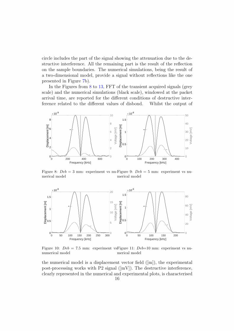
In the Figures from 8 to 13, FFT of the transient acquired signals (greyscale) and the numerical simulations (black scale), windowed at the packetarrival time, are reported for the different conditions of destructive inter-ference related to the different values of disbond. Whilst the output of

0 200 400 600Frequency [kHz]

0

2

4

6

8

Dis

plac

emen

t [m

]

10-9

0

2

4

6

8

10V

olta

ge [m

V]

Figure 8: Deb = 3 mm: experiment vs nu-merical model

0 100 200 300 400Frequency [kHz]

0

0.5

1

1.5D

ispl

acem

ent [

m]

10-8

0

10

20

30

40

50

Vol

tage

[mV

]

Figure 9: Deb = 5 mm: experiment vs nu-merical model

0 50 100 150 200 250 300Frequency [kHz]

0

0.5

1

1.5

Dis

plac

emen

t [m

]

10-8

0

5

10

15

20

Vol

tage

[mV

]

Figure 10: Deb = 7.5 mm: experiment vsnumerical model

0 50 100 150 200Frequency [kHz]

0

0.5

1

1.5

Dis

plac

emen

t [m

]

10-8

0

20

40

60

80

Vol

tage

[mV

]

Figure 11: Deb=10 mm: experiment vs nu-merical model

the numerical model is a displacement vector field ([m]), the experimentalpost-processing works with P2 signal ([mV]). The destructive interference,clearly represented in the numerical and experimental plots, is characterised

16

by a strong amplitude attenuation at the exciting frequency νatt (verticaldotted line in Figures) related to the specific value of disbond. The shape ofthe attenuated signals deviate from the bell-shape (Figure 4) of the originalexcitation.

0 50 100 150Frequency [kHz]

0

0.5

1

1.5

Dis

plac

emen

t [m

]

10-8

0

5

10

15

20

Vol

tage

[mV

]

Figure 12: Deb=12.5 mm: experiment vsnumerical model

0 50 100 150Frequency [kHz]

0

0.5

1

1.5

2

Dis

plac

emen

t [m

]

10-8

0

2

4

6

8

10

Vol

tage

[mV

]

Figure 13: Deb=15 mm: experiment vs nu-merical model

These plots are characterised by cusps that mean frequency values withvery low amplitude and assume a two bell-shape frequency spectrum. Fromthese Figures it is possible to highlight a high correlation between numericaland experimental results confirming what provided by Table 1. The erroris below 10% except for the case with 15 mm (which represents the 50% ofthe total bond length) and 3 mm of debonding.

In Figure 14 the numerical wave lengths, in circle markers, are reportedwith a linear interpolation formula (intercept equal to zero and dotted linein Figure); experimental results are reported in diamond markers. The slopevalue, SLJ specific feature, is used to evaluate the debonding length Debev(coming from experimental wave lengths λatt).

Experiments and numerical simulations were performed using toneburstwith central frequency other than νatt. For these situations the wave packetpreserved the original profile (and thus the frequency spectrum). Theseresults were not reported in the paper for the sake of conciseness.

6. Conclusions

This article presents a novel numerical model for wave motion in mediawith space dependent properties. Cauchy–Navier’s equations for elastody-namics were solved, in terms of finite differences, for a thin plate (SLJ)

17

0 2.5 5 7.5 10 12.5 15 17.5Debonding [mm]

0

15

30

45

60

75

Wav

e Le

ngth

at

t [mm

]

att = 4.3111deb

FD ModelExperiment

Figure 14: Debonding, attenuation wave length chart

excited by Lamb waves. The presence of an overlap zone with damage(debonding) was simulated with a piecewise-constant function describingthe wave propagation velocity (dependent on the density). Modulated tonebursts were used to excite the joint and this excitation was modelled by asource point in the finite differences model. The joint spectral response wascarefully investigated to relate the damage, artificially realised, with thesignal content. Numerical simulations and experimental campaigns wereconducted to validate the developed model and signal attenuation at spe-cific frequencies for each value of disbond was found representative of thedamage. Every frequency νatt was associated with a wave length in theattenuated signal: a linear relationship between λatt and Deb was found.

It is worth to remark that the observed coincidence of numerical simula-tions and experimental results occurs in spite of the more simple geometryof the numerical model. This is probably due to the presence of a discretesymmetry property of the solution across the bonded region. However, atthe moment this statement shall be regarded as a conjecture as a mathe-matical proof o it is yet to be found.

There are several reasons that make the method interesting. First ofall, the method based on a Finite Difference modelling is relatively simple.Numerical simulations like the ones presented in this manuscript can beimplemented in any programming language (Matlab was used, but Octavewould do the same job and is free) and run on any computer, as they are

18

not resource-consuming. Then, the proposed approach reveals the damagelength by using particular exciting frequencies. In the authors’ opinion,the elegance, simplicity and low cost of the method make it particularlyinteresting for industrial applications.

Acknowledgements

The ahthors are grateful to G. Saccomandi and K. Khusnutdinova foruseful suggestions. This research has been supported by the Departmentof Innovation Engineering and Department of Mathematics and Physics ofthe Universita del Salento. RV also acknowledges the support of GNFMof the Istituto Nazionale di Alta Matematica (Italy) and of the Italian Na-tional Institute for Nuclear Physics INFN, IS-CSN4 Mathematical Methodsof Nonlinear Physics.

References

[1] Alterman, Z., Loewenthal, D., 1970. Seismic waves in a quarter and three-quarterplane. Geophysical Journal of the Royal Astronomical Society 20 (2), 101–126, http://dx.doi.org/10.1111/j.1365-246X.1970.tb06058.x.

[2] Balasubramanyam, R., Quinney, D., Challis, R., Todd, C., 1996. A finite-differencesimulation of ultrasonic Lamb waves in metal sheets with experimental verification.Journal of Physics D: Applied Physics 29 (1), 147, https://doi.org/10.1088/

0022-3727/29/1/024.[3] Balvantın, A. J., Diosdado-De-la-Pena, J. A., Limon-Leyva, P. A. and Hernandez-

Rodrıguez, E., 2018. Study of guided wave propagation on a plate between twosolid bodies with imperfect contact conditions. Ultrasonics, 83, 137–145, https:

//doi.org/10.1016/j.ultras.2017.06.003

[4] Carrino, S., Nicassio, F., Scarselli, G., 2018. SHM of aerospace bonded structureswith improved techniques based on NEWS. In: Health Monitoring of Structural andBiological Systems XII. Vol. 10600. International Society for Optics and Photonics,p. 106002B, https://doi.org/10.1117/12.2300350.

[5] Dreiden, G V and Khusnutdinova, K R and Samsonov, A V and Semenova, I V(2012). Bulk strain solitary waves in bonded layered polymeric bars with delamina-tion. J. Appl. Phys. 112, 063516, http://dx.doi.org/10.1063/1.4752713.

[6] Donskoy, D., Sutin, A., Ekimov, A., 2001. Nonlinear acoustic interaction on contactinterfaces and its use for nondestructive testing. Ndt & E International 34 (4), 231–238, https://doi.org/10.1016/S0963-8695(00)00063-3.

[7] Fan, Z., Lowe, M. J., 2009. Elastic waves guided by a welded joint in a plate. In:Proceedings of the Royal Society of London A: Mathematical, Physical and Engi-neering Sciences. The Royal Society, pp. rspa–2009, https://doi.org/10.1098/

rspa.2009.0010.[8] Ginzburg, D., Ciampa, F., Scarselli, G., Meo, M., 2017. SHM of single lap adhe-

sive joints using subharmonic frequencies. Smart Materials and Structures 26 (10),105018, https://doi.org/10.1088/1361-665X/aa815c.

19

[9] Giurgiutiu, V., 2014. Wave Propagation SHM with PWAS Transducers. In: Struc-tural Health Monitoring with Piezoelectric Wafer Active Sensors: with Piezo-electric Wafer Active Sensors. Elsevier, pp. 639–706, https://doi.org/10.1016/C2013-0-00155-7.

[10] Gurtin, M. E., 1973. The linear theory of elasticity. In: Linear theories of elas-ticity and thermoelasticity. Springer, pp. 1–295, http://dx.doi.org/10.1007/

978-3-662-39776-3_1.[11] Heidarpour, F., Farahani, M., Ghabezi, P., 2018. Experimental investigation of the

effects of adhesive defects on the single lap joint strength. International journalof adhesion and adhesives 80, 128–132, https://doi.org/10.1016/j.ijadhadh.2017.08.005.

[12] Huthwaite, P., 2016. Guided wave tomography with an improved scattering model.Proc. R. Soc. A 472 (2195), 20160643, https://doi.org/10.1098/rspa.2016.

0643.[13] Jankauskas, A., Mazeika, L., 2016. Ultrasonic guided wave propagation through

welded lap joints. Metals 6 (12), 315, https://doi.org/10.3390/met6120315.[14] Jin, J., Quek, S., Wang, Q., 2003. Analytical solution of excitation of Lamb waves in

plates by inter-digital transducers. In: Proceedings of the Royal Society of LondonA: Mathematical, Physical and Engineering Sciences. Vol. 459. The Royal Society,pp. 1117–1134, https://doi.org/10.1098/rspa.2002.1071.

[15] Kalkowski, M. K., Rustighi, E., Waters, T. P., 2016. Modelling piezoelectric exci-tation in waveguides using the semi-analytical finite element method. Computers &Structures 1, 173–186. https://doi.org/10.1016/j.compstruc.2016.05.022.

[16] Khusnutdinova, K. R., Samsonov, A. M., 2008. Fission of a longitudinal strainsolitary wave in a delaminated bar. Phys. Rev. E 77, 066603, https://doi.org/10.1103/PhysRevE.77.066603.

[17] Khusnutdinova, K. R, Tranter, M. R., 2018. On radiating solitary waves in bi-layerswith delamination and coupled Ostrovsky equations. Chaos, 27, 013112, http://dx.doi.org/10.1063/1.4973854.

[18] Khusnutdinova, K. R, Tranter, M. R., 2015. Modelling of nonlinear wave scatteringin a delaminated elastic bar. Proc. R. Soc. A, 471, 20150584, http://dx.doi.org/10.1098/rspa.2015.0584.

[19] Kijanka, P., Manohar, A., Lanza di Scalea, F., 2015. Damage location by ultrasonicLamb waves and piezoelectric rosettes. Journal of Intelligent Material Systems andStructures, 26, 12, https://doi.org/10.1177/1045389X14544140

[20] Kim, Y., Ha, S. and Chang, F. K., 2008. Time-domain spectral element methodfor built-in piezoelectric-actuator-induced lamb wave propagation analysis. AIAAjournal, 46 (3), 591–600, https://doi.org/10.2514/1.27046.

[21] Leonard, F., Stein, J., Soutis, C., Withers, P., 2017. The quantification of impactdamage distribution in composite laminates by analysis of X-ray computed tomo-grams. Composites Science and Technology 152, 139–148, https://doi.org/10.

1016/j.compscitech.2017.08.034.[22] Liu, X., Zhou, L., Ouyang, Q., 2016. Modeling of PZT-induced Lamb wave prop-

agation in structures by using a novel two-layer spectral finite element. In: Sen-sors and Smart Structures Technologies for Civil, Mechanical, and AerospaceSystems. Vol. 9803. International Society for Optics and Photonics, p. 98034D,

20

https://doi.org/10.1117/12.2218960.[23] Mahapatra, D. R. and Gopalakrishnan, S., 2004. Spectral finite element analysis

of coupled wave propagation in composite beams with multiple delaminations andstrip inclusions. International journal of solids and structures, 41(5–6), 1173–1208,https://doi.org/10.1016/j.ijsolstr.2003.10.018.

[24] Malinowski, P. H., Ostachowicz, W. M., Brune, K., Schlag, M., 2017. Study ofelectromechanical impedance changes caused by modifications of CFRP adhesivebonds. Fatigue & Fracture of Engineering Materials & Structures 40 (10), 1592–1600, https://doi.org/10.1111/ffe.12661.

[25] Marks, R., Clarke, A., Featherston, C., Paget, C., Pullin, R., 2016. Lamb waveinteraction with adhesively bonded stiffeners and disbonds using 3D vibrometry.Applied Sciences 6 (1), 12, https://doi.org/10.3390/app6010012.

[26] Montinaro, N., Cerniglia, D., Pitarresi, G., 2017. Detection and characterisation ofdisbonds on fibre metal laminate hybrid composites by flying laser spot thermogra-phy. Composites Part B: Engineering 108, 164–173, https://doi.org/10.1016/j.compositesb.2016.09.084.

[27] Mueller, E. M., Starnes, S., Strickland, N., Kenny, P., Williams, C., 2016. Thedetection, inspection, and failure analysis of a composite wing skin defect on atactical aircraft. Composite Structures 145, 186–193, https://doi.org/10.1016/j.compstruct.2016.02.046.

[28] Ong, W. H., Rajic, N., Chiu, W. K., Rosalie, C., 2018. Lamb wave–based detectionof a controlled disbond in a lap joint. Structural Health Monitoring 17 (3), 668–683,https://doi.org/10.1177/1475921717715302.

[29] Ren, B., Lissenden, C. J., 2018. Modeling guided wave excitation in plates withsurface mounted piezoelectric elements: coupled physics and normal mode expan-sion. Smart Materials and Structures 27 (4), 045014, https://doi.org/10.1088/1361-665X/aab162.

[30] Scarselli, G., Ciampa, F., Nicassio, F., Meo, M., 2017. Non-linear methods basedon ultrasonic waves to analyse disbonds in single lap joints. Proceedings of theInstitution of Mechanical Engineers, Part C: Journal of Mechanical EngineeringScience 231 (16), 3066–3076, https://doi.org/10.1177/0954406217704222.

[31] Scarselli, G., Corcione, C., Nicassio, F., Maffezzoli, A., 2017. Adhesive joints withimproved mechanical properties for aerospace applications. International Journalof Adhesion and Adhesives 75, 174–180, https://doi.org/10.1016/j.ijadhadh.2017.03.012.

[32] Scarselli, G., Nicassio, F., 2017. Analysis of debonding in single lap joints based onemployment of ultrasounds. In: Health Monitoring of Structural and Biological Sys-tems 2017. Vol. 10170. International Society for Optics and Photonics, p. 1017020,https://doi.org/10.1117/12.2260041.

[33] Solodov, I., Bai, J., Bekgulyan, S., Busse, G., 2011. A local defect resonance toenhance acoustic wave-defect interaction in ultrasonic nondestructive evaluation.Applied Physics Letters 99 (21), 211911, https://doi.org/10.1063/1.3663872.

[34] Solodov, I. Y., Krohn, N., Busse, G., 2002. CAN: an example of nonclassical acousticnonlinearity in solids. Ultrasonics 40 (1-8), 621–625, https://doi.org/10.1016/S0041-624X(02)00186-5.

[35] Yadav, V. B., Pramila, T., Raghuram, V., Kishore, N., 2006. A finite difference simu-

21

lation of multi-mode Lamb waves in aluminium sheet with experimental verificationusing laser based ultrasonic generation. In: Proceedings of the 12th Asia-Pacificconference on NDT. Citeseer, pp. 1–7.

[36] Yashiro, S., Wada, J., Sakaida, Y., 2017. A monitoring technique for disbond area incarbon fiber–reinforced polymer bonded joints using embedded fiber Bragg gratingsensors: Development and experimental validation. Structural Health Monitoring16 (2), 185–201, https://doi.org/10.1177/1475921716669979.

22