Finite Element Formulation for the Consolidation Process ...

Institute ofApplied MechanicsInstitut für Baumechanik

Masterarbeit im Studiengang Bauingenieurwissenachaftenam Institut für Baumechanik

Technische Universität Graz

Finite Element Formulation

for the Consolidation Process

in poro-elasto-plastic Media

Michael Gfrerer

Graz, September 2013

Betreuer: Univ.-Prof. Dr.-Ing. Martin Schanz

mitbetreuender Assistent: Dipl.-Ing. Franz Rammerstorfer

Statutory Declaration

I declare that I have authored this thesis independently, that I have not used other than thedeclared sources/resources, and that I have explicitly marked all material which has beenquoted either literally or by content from the used sources.

Graz,

Date Signature

Eidesstattliche Erklärung1

Ich erkläre an Eides statt, dass ich die vorliegende Arbeit selbstständig verfasst, andere alsdie angegebenen Quellen/Hilfsmittel nicht benutzt, und die den benutzten Quellen wörtlichund inhaltlich entnommenen Stellen als solche kenntlich gemacht habe.

Graz, am

Datum Unterschrift

1Beschluss der Curricula-Kommission für Bachelor-, Master- und Diplomstudien vom 10.11.2008; Geneh-migung des Senates am 1.12.2008

Abstract

The mechanical behavior of soils can be strongly influenced by water present in the poresbetween the solid grains. This interaction can have significant influence on the design pro-cess in geotechnical engineering. An example would be the settlement of a foundation.Also in other areas of engineering the behavior of porous media is important, for instancewhen gas saturated foams or biological tissues are studied. Simulations of porous mediaare a difficult task for modeling as well as for numerical treatment. In this work, the numer-ical realization of Biot’s consolidation model with the finite element method is presented.Additionally to Biot’s model, the solid skeleton is allowed to deform elastic-plastic. Dueto plastic deformations the problem gets nonlinear. For the implemented plasticity modelsof Drucker-Prager and von Mises a consistent linearization is performed analytically. Theresult is a super-linear convergent newton-like solver. The discretization of the coupledproblem leads to a block-system of linear equations. This system is solved by an iterativesolver of simple type suitable for saddle point problems relying on two linear solvers forthe decoupled solid problem and fluid problem.

Zusammenfassung

In einem wassergesättigten Boden kann die Interaktion zwischen den Körnern und demWasser großen Einfluss auf das mechanische Verhalten haben und ist daher bei der Aus-legung von Bauwerken zu berücksichtigen. Im Allgemeinen ist die Simulation von po-rösen Medien sowohl in Fragen bezüglich der Modellierung als auch deren numerischerUmsetzung herausfordernd. In dieser Arbeit wird das Konsolidierungsmodell von Biotmithilfe der Finiten Elemente Methode gelöst. Zusätzlich zu dem Model von Biot wirdein elastisch-plastisches Verhalten des Festkörperskeletts angenommen. Im Fall von tat-sächlich auftretenden plastischen Verformungen wird das Problem nichtlinear, zu dessenLösung ein quasi-Newtonverfahren angewandt wird. Eine konsistente Linearisierung desplastischen Anteils ergibt eine Methode mit super-linerarer Konvergenz. Das gekoppelteFluid-Festkörperproblem führt auf ein Blocksystem an linearen Gleichungen welches ite-rativ gelöst wird. Dabei wird beachtet, dass im undrainierten Grenzfall das System einSattelpunktproblem darstellt.

CONTENTS

1. Introduction 11.1. Remarks on the notation . . . . . . . . . . . . . . . . . . . . . . . . . . 21.2. Outline of the work . . . . . . . . . . . . . . . . . . . . . . . . . . . . . 3

2. Fundamentals of Continuum Mechanics and Biot’s Theory of Porous Media 52.1. Geometry . . . . . . . . . . . . . . . . . . . . . . . . . . . . . . . . . . 5

2.1.1. Body . . . . . . . . . . . . . . . . . . . . . . . . . . . . . . . . 52.1.2. Deformation gradient . . . . . . . . . . . . . . . . . . . . . . . . 62.1.3. Strain measures . . . . . . . . . . . . . . . . . . . . . . . . . . . 8

2.2. Kinetics . . . . . . . . . . . . . . . . . . . . . . . . . . . . . . . . . . . 92.2.1. Load . . . . . . . . . . . . . . . . . . . . . . . . . . . . . . . . 92.2.2. Stress state and the Cauchy Stress Tensor . . . . . . . . . . . . . 102.2.3. Other stress measures . . . . . . . . . . . . . . . . . . . . . . . . 11

2.3. Constitutive relations . . . . . . . . . . . . . . . . . . . . . . . . . . . . 112.3.1. Elasticity . . . . . . . . . . . . . . . . . . . . . . . . . . . . . . 122.3.2. Plasticity . . . . . . . . . . . . . . . . . . . . . . . . . . . . . . 132.3.3. Theory of saturated porous media . . . . . . . . . . . . . . . . . 15

2.4. Balance laws . . . . . . . . . . . . . . . . . . . . . . . . . . . . . . . . 172.4.1. Preliminary theorems . . . . . . . . . . . . . . . . . . . . . . . . 172.4.2. Master balance law . . . . . . . . . . . . . . . . . . . . . . . . . 182.4.3. Conservation of mass . . . . . . . . . . . . . . . . . . . . . . . . 192.4.4. Balance of momentum . . . . . . . . . . . . . . . . . . . . . . . 202.4.5. Balance of moment of momentum . . . . . . . . . . . . . . . . . 202.4.6. Balance equations for a biphase medium . . . . . . . . . . . . . 21

3. Boundary Value Problems 233.1. Differential form of boundary value problems . . . . . . . . . . . . . . . 233.2. Weak form of boundary value problems . . . . . . . . . . . . . . . . . . 26

4. Solution Methods and Algorithms 294.1. Solution of the plastic evolution problem . . . . . . . . . . . . . . . . . . 29

4.1.1. General closest point projection . . . . . . . . . . . . . . . . . . 294.1.2. Specialization to the von Mises yield criterion with linear isotropic

hardening . . . . . . . . . . . . . . . . . . . . . . . . . . . . . . 324.1.3. Specialization to the non-associative Drucker-Prager model . . . 33

i

4.2. Basics of the Finite Element Method . . . . . . . . . . . . . . . . . . . . 344.3. A Newton-like FEM for the incremental elasto-plastic problem . . . . . . 364.4. Solution procedure for the elasto-plastic consolidation problem . . . . . . 41

5. Examples 455.1. Circular tube . . . . . . . . . . . . . . . . . . . . . . . . . . . . . . . . 455.2. Poro-elastic column . . . . . . . . . . . . . . . . . . . . . . . . . . . . . 475.3. Footing . . . . . . . . . . . . . . . . . . . . . . . . . . . . . . . . . . . 48

6. Conclusion 55

A. Space, Frames and Tensors 57

References 61

ii

1. INTRODUCTION

What is consolidation? Imagine, standing at the sea and looking at the horizon. Yourfeet will sink in the wet sand. You are experiencing consolidation. Walking further andlooking back you see that the footprints in the sand stay present. You have deformed thesand plastically. More engineering relevant consolidation processes in connection withplastic material behavior can be found in geotechnics. The settlement of foundations orthe construction of dams are examples where the interaction of the soil and the infiltratedwater can have significant influence on the behavior of the construction. Building a damto fast can cause failure because of this interaction. Not only in geotechnics, also in otherengineering fields like civil engineering or biomechanics simulation of porous materials isbecoming more and more important.

A state of the art approach in modeling is to consider the material as continuum. Thismeans that the body of interest is described as a set of continuously connected points inspace. Physical quantities like displacements or pressure are treated as fields on a macro-scopic level. For bodies undergoing reversible deformations the well established theoryof elasticity exists. On the other hand to account for irreversible deformations differ-ent plasticity models has been developed. Beside the classical models of von Mises andTresca complex models exist to describe the behavior of soils (see e.g. the textbook of Yu[38]). For continuum mechanics a huge amount of books and textbooks are available. Thebooks Altenbach [1], Marsden and Hughes [20], Truesdell and Noll [30] and Truesdell andToupin [31] are some examples.

In the last century, the classical theory of continua has been extended to account for porousstructures in materials. Today, three main theories can be found for modeling porousmaterials. The earliest approach is Biot’s Theory (BT) which is based on the work of vonTerzaghi [32]. In a series of papers it has been developed and improved by Biot [5],[6],[7], [8]. It will be used in this work.

The Theory of Porous Media (TPM) is based on the theory of continua for mixtures, ex-tended by the concept of volume fractions by Bowen [11], [10]. A historical review of theTPM is given by de Boer [14]. A large scale computation using the TPM with a complexplasticity model is given by Wieners et al. [33]. A comparison of the BT and the TPM canbe found in Schanz and Diebels [26].

As a third theory, the Simple Mixture Model (SMM) of Wilmanski [35] is also able todescribe porous media. Although, it is based on the fundamental laws of thermodynamics,it neglects some effects which are captured within the BT.

1

2 1. Introduction

In case of two or three dimensional models analytic solutions are only available in specialcases, e.g. see the review articles of Schanz [25] and Selvadurai [27]). Therefore, methodshave been developed to obtain a numerical solution. Beside others, the Finite DifferenceMethod (FDM), the Boundary Element Method (BEM) and the Finite Element Method(FEM) are well established methods. Within this work the FEM will be used. The booksof Braess [12], Jung and Langer [18], Wriggers [37], Zienkiewicz [39] are only someexamples of available textbooks on the topic.

The FEM is based on a variational formulation of the governing partial differential equa-tions. Therefore, integration over the computational domain is necessary. Normally, theseintegrals are treated with a quadrature rule, e.g. Gauss integration. As a standard approachfor the incorporation of plasticity, as a first step the stress response is calculated at thequadrature points. Second, on the basis of the calculated stress it is checked whether theresponse is elastic or plastic. In case of a plastic response a return mapping algorithm hasto be applied. A large class of return map algorithms are analyzed in [22]. For the globalnonlinear problem a newton like method has to be applied. The use of a so called consis-tent tangent operator introduced by Simo and Taylor [29] yields super-linear convergence.This is proven by Gruber et al. [23] and Sauter and Wieners [24] for different plasticitymodels.

Within this work a different approach is presented. The plastic strains are also approxi-mated with shape functions, as the displacement field is. Instead of performing the returnmap algorithm at the quadrature points it is performed at the nodes of the plastic strainapproximation. Furthermore, a consistent linearization yielding a super-linear convergentnewton like method is presented.

1.1. Remarks on the notation

In this work symbolic notation as well as index notation will be used.

Notation. (Index notation) The components of a first order tensor u are written as uiwhereas the components of a second order tensor T are written as Ti j. Higher ordertensors are written analogously. In general, any index i, I, j,J,k,K, . . . take on the values1,2,3.

Furthermore, Einstein summation convention will be used frequently.

Notation. (Summation convention) If an index occurs twice in an product expression thesummation over this index is taken from one to three. The summation sign ∑ is omitted,

r = riei = r1e1 + r2e2 + r3e3

1.2. Outline of the work 3

The Kronecker delta δi j denotes the components of the second order identity tensor withthe property

δi j =

1 if i = j0 if i 6= j

.

The derivative of a tensor T with respect to a space coordinate xi is denoted by T,i. It isassumed that xi refers to an orthonormal Cartesian basis. The derivative with respect totime is denoted as T .

1.2. Outline of the work

In chapter 2, the fundamentals of continuum mechanics and Biot’s Theory are described.First considerations of geometric aspects of the behavior of bodies ending with the in-troduction of strain measures are given. This is followed by a short section on kinetics.Next, basic constitutive models for elasticity and plasticity are introduced. Finally, bal-ance equations for mass, momentum and moment of momentum are stated. In chapter 3,the governing equations in connection with boundary data lead to boundary value prob-lems. In chapter 4, the used algorithms and methods for solving the problem of porouselasto-plastic materials are described. Chapter 5 finishes this thesis with the validation ofthe implemented program and a numerical example.

4 1. Introduction

2. FUNDAMENTALS OF CONTINUUM MECHANICS ANDBIOT’S THEORY OF POROUS MEDIA

This chapter introduces the continuum mechanical background and Biot’s theory of porousmedia. Firstly, the geometric description of a physical object is introduced. This is fol-lowed by a section on kinetics. Next, constitutive equations are given for elastic and plasticmaterial behavior and fluid flow (Law of Darcy). Finally, the balance equations for mass,momentum and moment of momentum are given.

2.1. Geometry

This section introduces the geometric description of the physical objects which will betreated in this work. First, the concept of representing bodies as connected points is in-troduced. In order to describe local properties of the change in geometry, the so-calleddeformation gradient is introduced. Finally, with the motivation to connect geometry andforce, which are responsible for a change in geometry, a quantity called strain is extractedfrom the deformation gradient. Basic considerations from classical mechanics about spaceof observation, frames and tensors are given in the appendix A.

2.1.1. Body

The physical objects of consideration in this work are continuous media with physicalproperties embedded in the three-dimensional Euclidean space. Whether the whole objector parts of it are called body, which is introduced as follows.

Definition 1. (Body) A body is an open set S ⊂ R3 and its boundary is as smooth asrequired.

The final goal in this work is to study the behavior (the movement and the change of shape)of bodies which are influenced by forces. For now the reasons for the forces remainsunmentioned. Therefore, a particular state of the object is chosen to be reference forsubsequent behave of the object. This state is called the reference configuration and will bedenoted by B. In the following a point of the reference (material) configuration is denotedby X ∈ B and called a material point. The geometry of any state of the object can then bedescribed by a mapping called deformation.

5

6 2. Fundamentals of Continuum Mechanics and Biot’s Theory of Porous Media

Definition 2. (Deformation) A deformation is a invertible B→ S map, which is as smoothas required. Therefore,

φ : B→ Sx = φ(X),

φ−1 : S→ B

X = φ−1(x),

where φ−1 denotes the inverse.

The configuration at a fixed time t > 0 is called current (spatial) configuration and a pointx ∈ S is called a spatial point. In the following, transformations which relate physicalquantities of the reference configuration to the current configuration are investigated. IfXI is a coordinate system on the reference configuration and xi is a coordinate systemon the current configuration, then a quantity QA...Za...z is called a two point tensor of ordern. For the numerical treatment of problems in continuum mechanics it is convenient tointroduce the displacement as the difference of the current configuration and the referenceconfiguration,

u(X) = φ(X)−X . (2.1)

2.1.2. Deformation gradient

In the following, a tensor describing the deformation at a material point and its infinites-imal neighborhood is introduced. This tensor is called deformation gradient and plays afundamental role in continuum mechanics. Before a definition is made, an example illus-trating a deformation is given.

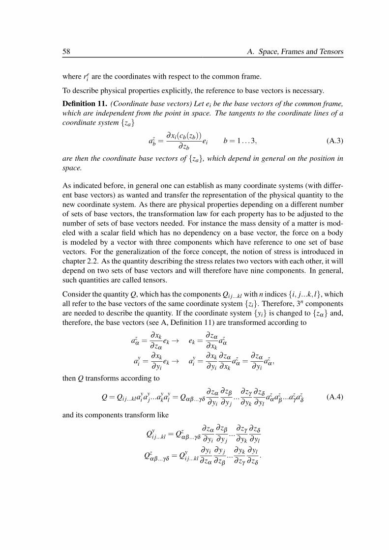
Example. (Example Deformation) Choosing a rectangular Cartesian coordinate systemfor all following considerations. Let the deformation φ : R3→ R3

x1(X) = X1 +(e2X2−1+0.7(X1)

3)

20

x2(X) = X2−(eX1−1+0.7(X2)

3)

10x3(X) = X3

be given. Consider a straight line l(t) = A+(B−A)t from A = [0,0,0]> to B = [1,1,0]>.Applying the deformation on l yields the curve c(t) = φ(l(t)). A Taylor series of φ at Ais made. The situation is visualized in figure 2.1. Obviously the approximating propertyof the Taylor’s Series can be seen. Furthermore, the deformed curve and all its approxi-mations share the same tangent at A. Therefore, to describe the deformation locally in ainfinitesimal neighborhood of A the first derivative is sufficient.

2.1. Geometry 7

A

B

Figure 2.1.: Plot of the deformation and its approximations

With the motivation of the previous example one defines the deformation gradient as fol-lows.

Definition 3. (Deformation Gradient) Let φ be a deformation of the reference body B.Then the two point tensor of order two,

FiJ(X) =∂φi(X)

∂XJX ∈ B (2.2)

is the deformation gradient of φ [20, p.48].

The deformation gradient F maps therefore infinitesimal line elements dX emigrating fromX ∈ B to its deformed configuration denoted by dx,

dxi = FiJdXJ. (2.3)

Due to the deformation a body can change its volume. This is investigated in the following.Consider a particle X of the reference configuration and the three infinitesimal vectors dA,dB and dC. These vectors span the infinitesimal volume

dV = (dA×dB) ·dC (2.4)

Mapping the vectors into a deformed configuration they read as F(X)da, F(X)db andF(X)dc. The deformed volume is now

dv = (FdA×FdB) ·FdC = det(F)dV (2.5)


Therefore, the local change in volume can be measured by

dvdV

= det(F(X)) =: J(X). (2.6)

At the reference configuration the deformation gradient is the identity, F = I and thereforeJ = 1. Furthermore, the existence of an inverse of the deformation requires J 6= 0. Togetherwith the requirement that a sequence of deformations in time has to be continuous [31], thecondition J > 0 follows. A similar consideration as for an infinitesimal volume elementholds for an area dA = dC×dD in the reference configuration. The corresponding area dain the deformed configuration is obtained by

da = det(F)F−>dA. (2.7)

For establishing constitutive relations it is convenient to have a strain measure which isinvariant for rigid body motions. With the deformation gradient a quantity is given, whichis invariant to rigid body translations but not to rigid body rotations. Applying the polardecomposition theorem [20, p. 51] the deformation gradient F(X) can be decomposedas

FiJ(X) = RiK(X)UKJ(X) =Vik(X)RkJ(X). (2.8)

In (2.8), R is a orthogonal tensor and called rotational tensor, U is the right stretch tensorand V is the left stretch tensor. The tensors U and V are now appropriate quantities todefine strain measures, because the information of rigid body rotations is solely containedin R. Using the fact that R is an orthogonal tensor one introduces the right Cauchy-Greentensor as

C(X) = FT (X)F(X) =UT (X)U(X), (2.9)

where no information of R is contained.

2.1.3. Strain measures

A major task in modeling is to find a suitable relation between the deformation of a con-tinuum and its stress state which will be introduced formally in section 2.2. Such relationsare called constitutive relations and will be treated in section 2.3. As indicated earlier, tostate an objective constitutive relation it must not depend on rigid body motions. As everystrain measure is a purely mathematical quantity every strain measure is equivalent to eachother. One of the most stated strain measures is the so called Green-Lagrange-Strain tensorwhich is introduced in the following definition.

Definition 4. (Green-Lagrange-Strain) The Green-Lagrange strain tensor E is defined as

Ei j =12(Ci j−δi j) =

12(ui, j +u j,i +ui,ku j,k), (2.10)

where C is the right Cauchy-Green tensor.

2.2. Kinetics 9

By neglecting nonlinear terms in the definition of the Green-Lagrange-Strain tensor the socalled linearized strain tensor is obtained.

Definition 5. (Linearized Strain) The linearized strain tensor is defined as

εi j =12(ui, j +u j,i). (2.11)

2.2. Kinetics

In section 2.1, the geometric description of a physical object is introduced. Thereby, nofurther specifications of the reasons responsible for the behavior has been made. In thischapter, the mechanical ones are introduced. Furthermore, the notion of stress and differentstress measures are introduced.

2.2.1. Load

The reason for the deformation of matter can have different reasons. From the set ofall possible reasons (for instance thermal, electromagnetic, chemical and others) only themechanical ones are treated here. These can be grouped in

• body loads and

• surface loads.

Here, body loads are related to the mass density of the body. The force density due to bodyloads f (x) is given by

f (x) = ρk, (2.12)

with the mass density ρ and a vector field k. The specialization for gravitation as the onlyone treated here reads

f (x) =−ρge3 (2.13)

with the gravitational acceleration g and the vector e3 pointing away from the center ofgravity. The resulting force Fb on a body due to body load can be computed by integrationover the volume of the body,

Fb =∫S

f (x)dx. (2.14)

The surface loads represent the interaction of two neighbored bodies on their common sur-face. To characterize this interaction the so called Cauchy traction vector as the respectiveforce surface density is introduced.


Definition 6. (Cauchy Traction Vector) Let S be a body with its boundary ∂S. Consider anoriented surface with the unit normal vector n(x) pointing outward of S and x ∈ ∂S. Thenthe vector t(x) representing the mechanical interaction between S and its surrounding iscalled the Cauchy traction vector at x.

The resulting force Fs on a body S due to surface loads can be computed by integrationover the surface of the body,

Fs =∫

∂S

t(x)da. (2.15)

Additionally to the notion of a resulting force, the resulting torque of a force acting at pointa with respect to the origin o is defined as

Θo = a×F. (2.16)

2.2.2. Stress state and the Cauchy Stress Tensor

As a point on the boundary of one body can also be on the boundary of other bodies butwith different surface normals the Cauchy traction vector is not unique. This motivates thedefinition of a stress state as follows.

Definition 7. (Stress State) The set of all traction vectors at a point x define the stress stateat that point.

Fortunately, the dependency of the Cauchy traction vector on the surface normal is linear,which tells the well known theorem of Cauchy.

Theorem 1. (Cauchy) The Cauchy traction vector t(x,n) at a fixed point x but arbitrarysurface normal vector n is given by

t(x,n) = σ(x)n, (2.17)

with the Cauchy stress tensor σ ,which is a second order tensor on the current configura-tion.

In view of theorem 1 the stress state is uniquely defined if the Cauchy stress tensor isknown.

2.3. Constitutive relations 11

2.2.3. Other stress measures

The Cauchy traction vector represents the actual force acting on an area in the currentconfiguration. As in most applications the current configuration is not known beforehand,the integration to get the resulting force can not be performed. Therefore, the domainof integration is transformed to the reference configuration. Take a deformation φ and areference body B. Then the current configuration S is given with φ(B). The resulting forcedue to surface loads is

Fs =∫

∂S

t(x)da =∫

∂S

σ(x)n(x)da =∫

∂B

σ(φ(X))n(φ(X))J(φ(X))dA. (2.18)

This motivates the following definition.

Definition 8. (Kirchhoff Stress) Let φ be a deformation with the deformation gradient Fand J = det(F). Furthermore, let σ the Cauchy stress tensor, then

τ = Jσ (2.19)

defines the Kirchhoff stress tensor.

Not only the domain can be transformed also the normal vector involved in equation (2.18)can be transformed to the reference configuration. This motivates the definition of the FirstPiola-Kirchhoff stress tensor P as

P = JσF−T (2.20)

As a last stress measure the Second Piola-Kirchhoff stress tensor S is introduced as

S = JF−1σF−T . (2.21)

2.3. Constitutive relations

As mentioned before, a constitutive relation closes the gap between stress state and strainstate. First, a general form of elastic constitutive relations (hyperelastic) which allow tomodel large strain behavior of many materials is given. Next, the equations for the specialcase of the linear elastic isotropic constitutive relation are given. Then, a section aboutplasticity introduces the classical rate independent plasticity theory, which will be spe-cialized to a non-associative Drucker-Prager model which contains the von Mises model.Finally, considerations about a two phase media are given. Thereby, one phase is a solidskeleton showing an elasto-plastic response, and the other phase is a fluid flowing throughthe pores of the solid. This section is based on [20] and [16] for elasticity, [17] for plasticityand on [5] for porous media.

In the following, the space of symmetric second order tensors is denoted by Ts.


2.3.1. Elasticity

Here, the class of hyperelastic constitutive models containing the linear elastic model ofHooke is given. For a hyperelastic constitutive relation there exists a stored energy func-tional W ,

W : Ts→ R (2.22)

such that the stress response σ at x ∈ S due to a given strain state ε ∈ Ts can be computedby

σ(x,ε) =∂W∂ε

(x,ε) x ∈ S,ε ∈ Ts. (2.23)

The second partial derivative of the functional W with respect to the strain tensor gives theso called elasticity tensor C which is a tensor of order four,

C(x,ε) =∂ 2W∂ε∂ε

(x,ε). (2.24)

As the determination of material parameters can be a difficult task one try to use the easiestconstitutive relation which gives sufficient results. The easiest elastic constitutive relationfor three dimensional modeling is obtained when only allowing a linear dependency ofthe stresses on the strains and assuming that the material response is equal in every di-rection (isotropic). Then the elasticity tensor has constant values depending on only twoparameters λ and µ ,

Ci jkl = λδi jδkl +µ(δikδ jl +δilδ jk). (2.25)

The stress can be computed by

σi j =Ci jklεkl = λ εkkδi j +2µεi j. (2.26)

The inversion of (2.26) yields the compliance relation

εi j =C−1i jklσkl =−

λ

2µ(3λ +2µ)σkkδi j +

12µ

σi j. (2.27)

With the definition of the Young’s modulus

E =µ(3λ +2µ)

λ +µ(2.28)

and Poisson’s ratio

ν =λ

2(λ +µ)(2.29)

the compliance relation (2.27) can be rephrased as

εi j =−ν

Eσkkδi j +

1+ν

Eσi j. (2.30)


Other useful constants are the bulk modulus

K = λ +23

µ =E

3(1−2ν)(2.31)

and the shear modulus G = µ .

2.3.2. Plasticity

For the behavior of metals the following can be observed. Before reaching a certain limitthe response can be modeled as linear elastic with high accuracy. Above this limit theresponse becomes nonlinear and inelastic, which means that after releasing the appliedload some deformations stay present. To determine whether the material is locally belowor above this limit, a yield criterion of the form

f (σ ,q) = Φ(σ ,q)−σy(q)≤ 0 (2.32)

is introduced. In equation (2.32) f is the yield function, Φ is a function which maps thestress state to a real number, σy is the yield strength and q is a set of internal variablesto model hardening response. The yield function has to be negative or zero. If it has annegative value the material has an elastic behavior, if it is zero the material yields. Asthe yielding of materials can influence the yield strength, the set of internal variables areintroduced to model the effects of the stress history. Recall that for a given deformationthe linearized strain can be computed by

εi j =12(ui, j +u j,i). (2.33)

In the theory of plasticity for small stains it is assumed that the total strain tensor in (2.33)can be additively decomposed into an elastic and a plastic part,

ε = εe + ε

p. (2.34)

The constitutive relation for a hyperelastic material is adjusted in such a way that it onlydepends on the elastic strains,

σi j =∂W (x,εe)

∂εei j

. (2.35)

For the plastic strain an evolution equation of the form

εp = γr(σ ,q) (2.36)

is assumed. This equation is called the flow rule. In (2.36), γ is the consistency parameterand r : Ts×Rm → Ts is a prescribed function defining the direction of the plastic flow.


For the special case r = ∂ f∂σ

the flow rule is called associative. Furthermore, the hardeninglaw

q =−γh(σ ,q) (2.37)

is a evolution law for the internal variables, where h : Ts×Rm→ Rm is a prescribed func-tion defining the type of hardening. In the associative case h = D∂ f

∂q with D containing thehardening moduli. In the following, conditions for the yield function and the consistencyparameter are given. In the case f < 0 the material behaves elastic, thus γ = 0. For f = 0plastic flow occurs according to (2.36). Therefore, γ 6= 0. As states with f > 0 are inad-missible f = 0 has to be valid in the case of plastic flow. Summarizing, the Kuhn-Tuckercomplementary condition

γ f (σ ,q) = 0 (2.38)

and the consistency conditionγ f (σ ,q) = 0 (2.39)

have to be fulfilled for all states.

A special yield creterion for isotropic material behavior is given by the Drucker-Prageryield criterion

f (σ) =

√12‖s‖+ pη−ξ c, (2.40)

where p and s are the hydrostatic stress state and the deviatoric stress state

p =13

σii,

si j = σi j− pδi j.(2.41)

Notation. (Tensor norm) The norm of the second order tensor s is defined as ‖s‖=√si jsi j.

In equation (2.40), η , ξ and c are material parameters. In this work, they are computed inthe way that an inner approximation of the Mohr-Coulomb yield criterion is achieved [15].Therefore, the friction angle and the cohesion are the input parameters for the implementedcode.

For the flow rule often the yield function is adopted to

f =

√12‖s‖+ pη , (2.42)

where η is computed with the dilatancy angle instead of the friction angle. Then the non-associative flow rule reads

εpkl = γ

∂ f∂σkl

= γ

(√12

skl

‖s‖+

13

ηδkl

). (2.43)


Neglecting the term containing the hydrostatic pressure p in equation (2.40) yields the vonMises yield criterion. Instead of using c as a material parameter the uniaxial yield strengthdenoted by σy,0 is used,

f =

√32‖s‖−σy,0−q, (2.44)

and the scalar isotropic hardening variable q is introduced. This yield criterion is basedon the assumptions that the occurrence of plastic flow is governed by the deviatoric stressenergy. The associative evolution of q is given by

q =−γD∂ f∂q

= γD, (2.45)

with the scalar isotropic hardening modulus D.

2.3.3. Theory of saturated porous media

Up to now, the physical body has been modeled as a single continuum. In this section, asuperposition of two continua is introduced. One is a solid skeleton and the other is a fluid.The following assumptions are made in the subsequent developments:

• the solid skeleton behaves isotropic

• the constitutive modeling of the solid skeleton is elastic-plastic

• the stress- strain relationship is linear in the elastic range

• only small strains occur, therefore the linearized strain tensor (2.11) is a appropriatestrain measure

• the fluid and the solid grains are incompressible

• the fluid flow through the pores of the solid skeleton is according to the Law of Darcy

To characterize the saturated porous media Coussy [13] distinguishes between the totalporosity and the connected porosity. The total porosity is defined as the ration of non-solidvolume to the total volume. In this work this quantity will not be used. The connectedporosity e f is the ratio of connected void space V f to the total volume V

e f =V f

V. (2.46)

It is assumed that the fluid can move freely through the connected void space, accordingto Darcy’s law. In the considered case of full saturation with one fluid, the volume fractionof the solid is given as

es = 1− e f . (2.47)


The mass density ρ of the bulk material is then given in terms of the mass densities of thesingle components

ρ = e fρ f + es

ρs, (2.48)

where ρ f is the mass density of the fluid and ρs is the mass density of the solid grains.

In the concept of partial stresses it is assumed that distinct stress tensors for the solid andfluid can be defined [6]. Then the total stress tensor σ tot is defined as

σtot = σ

s +σf , (2.49)

where σ s is the stress tensor for the solid and σ f is the stress tensor for the fluid. Theconstitutive equations for the solid

σsi j = 2µε

si j +

(λ +

Q2

R

)ε

skkδi j +Qε

fkkδi j, (2.50)

and the fluidσ

fi j = Qε

skkδi j +Rε

fkkδi j. (2.51)

are introduced. In [5], Biot shows that four independent physical constants are needed.In the equations (2.50) and (2.51) these are the two Lame parameters λ and µ describingthe solid and Q and R describe the coupling between the two phases. The parameters Qand R can be expressed in terms of the compression modulus of the solid grains Ks, thecompression modulus of the fluid K f , the compression modulus of the solid skeleton andthe porosity e f as

R =(e f )2K f (Ks)2

K f (Ks−K)+ e f Ks(Ks−K f )(2.52)

Q =e f (α− e f )K f (Ks)2

K f (Ks−K)+ e f Ks(Ks−K f )(2.53)

with Biot’s effective stress coefficient α = 1−K/Ks.

The stress state in the fluid is assumed to be hydrostatic. The relation between fluid stressand pore pressure p is defined by,

σf

i j =−e f pδi j. (2.54)

The minus sign is introduced because in elasticity a tensile stress is denoted positive, but apositive pore pressure is usually associated with an expansion of the pores. Due to a tensilestress the pores contract. That is why the pressure is defined as the negative hydrostaticfluid stress. Using Biot’s effective stress coefficient α the total stress is given as

σtoti j = 2µε

si j +λε

skkδi j−α pδi j. (2.55)

2.4. Balance laws 17

In the limiting case of incompressible solid grains α → 1. In view of equation (2.55), theeffective stress on the solid governing the elastic-plastic behavior is introduced as

σeffi j = σ

toti j +α pδi j. (2.56)

Furthermore, the variation of fluid volume per unit reference volume ζ is introduced

ζ = αεskk +

(e f )2

Rp. (2.57)

In case of incompressible constitutes it simplifies to

ζ = εskk. (2.58)

A relation between the velocity of the fluid and the pore water pressure is given by the lawof Darcy and has the form [19]

q = e f wi = e f k(ρ f gi− p,i). (2.59)

In equation (2.59), wi = u fi − us

i are the average relative velocity components, k is theisotropic permeability and g is the gravitational acceleration vector.

2.4. Balance laws

In section 2.2, the notion of force has been introduced. There different reasons for forcesare mentioned. Now in this chapter a balance law connects these forces in an equation.Equations of the same structure can be defined for the mass, linear momentum, angularmomentum, energy and an inequality of the same structure for entropy production. Fur-thermore, a balance law for the mass and the force in the fluid are given. This chapter isbased on [1], [19], [20] and [36].

2.4.1. Preliminary theorems

As a first theorem the divergence theorem is given, which allows to transform an volumeintegral into a surface integral.

Theorem 2. (Divergence Theorem) Let f be a vector field on S, then∫S

div f dx =∫

∂S

f nda (2.60)

holds. ∂S denotes the boundary of S and n the outward normal vector of ∂S.


The second theorem which will be needed in the further developments is the transporttheorem. It considers the rate of change in time of an value obtained by integration, wherenot only the integrand but also the domain of integration depends on time.

Theorem 3. (Reynold’s Transport Theorem) Let f be a given differentiable vector field onS, then

ddt

∫S

f dx =∫S

( f + f divv)dx =∫S

(∂ f∂ t

+div( f v))

dx =∫S

∂ f∂ t

dx+∫

∂S

n f vda (2.61)

holds. v denotes the velocity.

Equation (2.61) can be interpreted in that way that the rate of change of the quantity de-pends additive on two parts. The volume integral captures the change of the integrand andthe surface integral the change of the integration domain.

2.4.2. Master balance law

Let γ(x, t) be the density distribution of a mechanical quantity. The integration over thebody yields an extensive quantity Y,

Y (S, t) =∫S

γ(x, t)dx =∫B

γ(φ(X), t)J(X , t)dX =∫B

γ0(φ(X), t)dX (2.62)

with γ0 = γJ. This quantity can be measured in the laboratory. The rate of the mechanicalquantity with respect to time has to be in equilibrium with the external influence on therespective body. Therefore,

ddt

Y (S, t) =∫

∂S

θ(x,n, t)da+∫S

χ(x, t)dx (2.63)

has to hold, where θ is the surface density and χ is the volume density of the externalaction. d

dt denotes the material time derivative. For the surface densities θ a generalversion of the theorem of Cauchy (Theorem 1) holds. Therefore, the dependency of θ onthe normal vector n can be expressed as

θ(x,n, t) = θ(x, t)n, (2.64)

where θ is a tensor of one order higher than θ . Applying the transport theorem (2.61)yields the master balance law in integral form,∫

S

(∂γ

∂ t+div(γv)

)dx =

∫∂S

θ(x,n, t)da+∫S

χ(x, t)dx. (2.65)


Assuming all field variables in equation (2.65) are continuous. Then γ , θ and χ satisfyequation (2.65) if and only if they satisfy the local Eulerian master balance law

∂γ

∂ t+div(γv) = divθ +χ. (2.66)

This local form is obtained by transforming the surface integral to an volume integral withthe help of the divergence theorem. Since the master balance law holds for an arbitrarybody S the local form follows.

Also a local Lagrangian version of the master balance law is available. Therefore, theexternal actions are transformed to the reference configuration,∫

∂S

θ(x,n, t)da+∫S

χ(x, t)dx =∫

∂B

θ0(X ,n, t)dA+∫B

χ0(X , t)dX . (2.67)

withθ0 = θJF−T and χ0 = χJ.

The wanted result is obtained by applying the divergence theorem and using the arbitrayintegration domain

∂γ0(X , t)∂ t

= divθ0(X , t)+χo(X , t). (2.68)

In the following, the master balance law are specialized for mass, momentum and momentof momentum.

2.4.3. Conservation of mass

The total mass m of a body S is given by integration over its mass density ρ ,

m =∫S

ρ(x, t)dx =∫B

ρ0(X , t)dX (2.69)

Specifying the master balance law (2.68) and (2.66) for the mass and assuming no externalaction yields conservation of the mass in Lagrangian description

∂ρ0(X , t)∂ t

= 0 (2.70)

and Eulerian description

∂ρ(x, t)∂ t

+div(ρ(x, t)v(x, t)) = 0. (2.71)


2.4.4. Balance of momentum

The momentum p of a body S is given as

p =∫S

ρ(x, t)v(x, t)dx =∫B

ρ0(X , t)v(φ(X), t)dX . (2.72)

and relates velocity and mass density distribution. Postulating that force has an action onthe momentum the master balance law (2.65) gets the form

DpDt

=∫

∂S

t(x,n, t)da+∫S

f (x, t)dx (2.73)

where t are the Cauchy traction vector (see definition 6 in chapter 2.2) and f are the bodyload density introduced in equation (2.12). The localization of equation (2.73) gives thewell known relations [1]

divσ + f = ρDvDt

. (2.74)

for the Eulerian description and

divP+ f0 = ρ0∂v∂ t

(2.75)

for the Lagragian description, where the first Piola-Kirchhoff stress tensor P introduced inequation (2.20) is used.

2.4.5. Balance of moment of momentum

The momentum lo of a body S with respect to the origin o is given as

lo =∫S

x×ρv(x, t)dx, (2.76)

where x×ρv(x, t) is the cross product of the spatial position x and the momentum densityρv. Similar to the balance law of momentum one postulates that torque (2.16) has an actionon the moment of momentum. This gives the balance law,

DloDt

=∫

∂S

x× t(x,n, t)da+∫S

x× f (x, t)dx (2.77)

or equivalent in index notation

Dlok

Dt=∫

∂S

xit jεi jkda+∫S

xi f jεi jkdx. (2.78)


Using the mass conservation (2.70) and v× v = 0 the left-hand side can be evaluated to

DloDt

=∫S

x×ρDDt

v(x, t)dx =∫S

xiρDDt

v jεi jkdx, (2.79)

where εi jk is the Levi-Civita symbol with the property

εi j =

1 if (i, j, k) is an even permutation of (1,2,3)−1 if (i, j, k) is an odd permutation of (1,2,3)0 else

.

Using the Cauchy stress tensor and the divergence theorem, the surface integral on theright-hand side of (2.78) is transformed to a volume integral∫

∂S

xit jεi jkda =∫S

(xiσ jl,l + xi,lσilεi jk)dx (2.80)

Now (2.78) is rephrased as∫S

[ρ

DDt

v j−σ jl,l− f j

]xiεi jkdx =

∫S

xi,lσ jlεi jkdx. (2.81)

If the balance of momentum (2.74) holds, the left-hand side vanishes. It remains∫S

xi,lσ jlεi jkdx =∫S

δilσ jlεi jkdx =∫S

σ jiεi jkdx. (2.82)

This implies that the Cauchy stress tensor is symmetric.

2.4.6. Balance equations for a biphase medium

The same balance laws introduced have to hold for a biphase medium. For the mass bal-ance law no exchange between the phases is added and therefor for the solid part equation(2.70) stays valid. For the fluid the rate with respect to time of variation of fluid vol-ume per unit reference volume ζ introduced in equation (2.57) has to fulfill the continuityequation

ζ +wi,i = 0. (2.83)

Inserting the definitions for ζ in case of incompressible phases and the Law of Darcy (2.59)yields

εskk + k(ρ f g j− p, j),i = 0. (2.84)


As only consolidation processes are treated in this work the inertia terms are neglectedfrom the outset for the porous medium. In the momentum balance law the total stresstensor plays the crucial role,

σtoti j, j + fi = 0 (2.85)

wherefi = e f f f

i + es f si (2.86)

accounts for body loads. Using the definition of the total stress tensor (2.55) gives[σ

effi j − pδi j

], j+ fi = 0 (2.87)

in case of incompressible phases.

3. BOUNDARY VALUE PROBLEMS

This chapter summarizes the concepts developed so far which leads in connection withboundary data to boundary value problems. Excluding problem 1 in section 3.1, whichoutlines a possible extension of this work, only the geometric linear case is treated. There-fore, the difference between reference and current configuration is negligible. Hence, inthe following the domain which is occupied by the physical object is denoted by Ω andfixed during calculation. The boundary of Ω is Γ. Furthermore, no distinction betweendifferent stress or strain measures is made. The stress tensor will be σ and the strain tensorε in the rest of this work.

For the subsequent derivations the definition of the following function spaces are needed.The space of p-times continuous differentiable functions is denoted

Cp(Ω,Rd) = f : Ω⊂ R3→ Rd | f p-times continuously differentiable. (3.1)

Furthermore, the space of integrable functions is introduced as

Lp(Ω,Rd) = f : Ω⊂ R3→ Rd |∫Ω

[ f (x)]pdx < ∞. (3.2)

A generalization of the concept of differentiability leads to so called weak derivatives. Theintegrable function w∈L2(Ω,R) is called weak derivative of order m= |α|=α1+ · · ·+αdof the function u if ∫

Ω

u(x)∂ αφ

∂xα11 . . .∂xαd

ddx = (−1)|α|

∫Ω

w(x)φ(x) dx (3.3)

holds for all φ ∈C∞(Ω,R) with compact support [18]. The so called Sobolev space is thengiven as

Hp(Ω,Rd) = f ∈ L2(Ω,Rd) | f has weak derivatives w ∈ L2(Ω,Rd) up to order p.(3.4)

3.1. Differential form of boundary value problems

In this section, the differential or strong form of boundary value problems for nonlinearelasticity, linearized elasticity, elasto-plasticity and poro-elasto-plastic consolidation aregiven.

23

24 3. Boundary Value Problems

Problem 1. (Nonlinear Elasticity) Find the displacement field u ∈ C2(Ω,R3)∩C1(Ω∪Γt ,R3)∩C0(Ω,R3) such that the balance of momentum

σi j, j(u(x))+ fi(x) = 0 hold ∀x ∈Ω,

the Dirichlet boundary conditions

u(x) = uΓ(x) hold ∀x ∈ Γu,

and the Neumann boundary conditions

σ(x)n(x) = tΓ(x) hold ∀x ∈ Γt .

In the balance of momentum f ∈ C0(Ω,R3) is a prescribed function for body loads andthe Cauchy stress tensor σ is given through a hyperelastic constitutive relation

σi j =∂W (E)

∂Ei jwith Ei j =

12(ui, j +u j,i +ui,ku j,k).

uΓ ∈C0(Γu,R3) is a function of prescribed displacements on a part Γu of the boundary andtΓ ∈ C1(Γt ,R3) is a function of prescribed traction vectors on the part Γt of the boundary.For Γu and Γt hold

Γu∪Γt = Γ , Γu∩Γt = /0.

Using the linearized displacement-strain relation (2.11) and the constitutive model for alinear elastic isotropic material (2.26) the boundary value problem 1 can be simplified.

Problem 2. (Linearized Elasticity) Let f ∈ C0(Ω,R3). Find the displacement field u ∈C2(Ω,R3)∩C1(Ω∪Γt ,R3)∩C0(Ω,R3) such that

µui, j j(x)+(λ +µ)u j,i j(x)+ fi(x) = 0 hold ∀x ∈Ω,

and the boundary conditions analogously to problem 1 are fulfilled.

Additionally to the elastic material response an plastic response is added. Since only rateindependent plasticity is considered, time is considered in a pseudo sense. The boundaryvalue problem assuming small strains reads as follows.

Problem 3. (Elasto-Plasticity) Let f ∈C0(Ω,R3). Find the displacement field u∈C2(Ω,R3)∩C1(Ω∪Γt ,R3)∩C0(Ω,R3) such that

σi j, j(x)+ fi(x) = 0 hold ∀x ∈Ω,

and the boundary conditions analogously to problem 1 are fulfilled. The stress tensor isgiven as

σi j = λεekkδi j +2µε

ei j

3.1. Differential form of boundary value problems 25

with the elastic strain tensor

εei j =

12(ui, j +u j,i)− ε

pi j.

The evolution of the plastic strain tensor ε p is given as

εp =

0, if f (σ ,q)≤ 0γr(σ ,q), if f (σ ,q) = 0,

where f is an appropriate yield function, q is a set of appropriate internal variables whoseevolution is determined by

q =

0, if f (σ ,q)≤ 0γh(σ ,q), if f (σ ,q) = 0.

The functions r and h determine the respective direction of the evolution. The consistencyparameter γ and the yield function f have to fulfill

γ f = 0 and if f = 0 → γ f = 0.

Finally, the so call u-p form of the poro-elasto-plastic consolidation problem is given. Inaddition to problem 3 a fluid phase is present and the interaction with the solid is consid-ered. As consolidation is a process where real time matters, the time interval T = (0, t f inal)of interest is introduced. Other than the problems stated so far, the following problem is ainitial boundary value problem.

Problem 4. (Poro-Elasto-Plastic Consolidation) Let f ∈C0(Ω×T,R3). Find the pressurefield p ∈ C2(Ω× T,R)∩C1(Ω∪Γq× T,R)∩C0(Ω× T,R) and the displacement fieldu ∈ C2(Ω×T,R3)∩C1(Ω∪Γt×T,R3)∩C0(Ω×T,R3) such that the fluid mass balance

−[

k(p,i− fi)+∂ui

∂ t

],i= 0 hold ∀(x, t) ∈Ω×T

the momentum balance[σ

effi j − pδi j

], j+ fi = 0 hold ∀(x, t) ∈Ω×T,

the boundary conditions

u(x, t) = uΓ(x, t) hold ∀(x, t) ∈ Γu×T,σ

tot(x, t)n(x) = tΓ(x, t) hold ∀(x, t) ∈ Γt×T,p(x, t) = pΓ(x, t) hold ∀(x, t) ∈ Γp×T,

q(x, t)n(x) = qΓ(x, t) hold ∀(x, t) ∈ Γq×T

and the initial conditions

u(x,0) = u0 hold ∀x ∈Ω,

p(x,0) = p0 hold ∀x ∈Ω.

For the effective stress tensor σ eff the same relations as in problem 3 hold.


3.2. Weak form of boundary value problems

For a numerical solution it is preferred to recast the given boundary value problems into aweak (integral) form. This is done for problem 4. This section is according to the textbooks[18] and [37].

As a first step the spaces V u0 and V p

0 of test functions are introduced as

V u0 = ξ (x) ∈H1(Ω,R3) | ξ (x) = 0 ∀x ∈ Γu,

V p0 = η(x) ∈H1(Ω,R) |η(x) = 0 ∀x ∈ Γp.

(3.5)

The weak equilibrium equations are obtained as follows. Starting from the local equilib-rium equation and multiply it with a vector-valued test function ξ ∈V u

0 and integrate overthe computational domain Ω,∫

Ω

[(σ

effi j, j− p, jδi j

)ξi + fiξi

]dx = 0. (3.6)

Applying integration by parts and divergence theorem on the effective stress and the porepressure yields ∫

Ω

[−σ

effi j ξi, j + pξ j, j + fiξi

]dx+

∫∂Ω

t toti ξi dx = 0. (3.7)

Remark. As the stress tensor is symmetric (σi j = σ ji) any antisymmetric part of ξi, j hasno contribution to σi jξi, j. Therefore,

σi jξi, j = σi j12(ξi, j +ξ j,i)+σi j

12(ξi, j−ξ j,i) = σi j

12(ξi, j +ξ j,i)

holds. In the engineering literature (e.g. [39]) this relation is used to introduce the notionof virtual strain δε = 1/2(ξi, j +ξ j,i).

The space of the test functions is chosen in a way that it contains only functions of valuezero on the Dirichlet boundary Γu. Therefore, the part of the boundary where displace-ments are prescribed and the traction are unknown are eliminated in the last integral of(3.7). The final weak equilibrium equations reads∫

Ω

σeffi j ξi, j dx−

∫Ω

pξ j, j dx = F(ξ ) (3.8)

with the linear formF(ξ ) =

∫Ω

fiξi dx+∫Γt

t toti ξi dx

3.2. Weak form of boundary value problems 27

containing only known data.

The weak form of the balance of mass is obtained analogously. Multiplication with ascalar-valued testfunction η p ∈V p

0 and integration over the domain gives∫Ω

[k(p,i− fi)+ ui],i η dx = 0. (3.9)

Applying integration by parts and divergence theorem yields

−∫Ω

k(

p,i− fi)η

p,i dx+

∫∂Ω

k(

p,i− fi)niη dx+

∫Ω

ui,iη dx = 0. (3.10)

Again, the restriction of the test functions η to functions with value zero on Γp and usingthe Law of Darcy q = k

(p,i− fi

)ni gives the final equation∫

Ω

k p,i η,i dx−∫Ω

ui,iη dx =∫Ω

k f fi η,i dx+

∫Γq

qη dx. (3.11)

The results of this section are summarized in the statement of the weak consolidationproblem which will be solved in chapter 4.

Problem 5. (Weak Poro-Elasto-Plastic Consolidation) Let f ∈ L2(Ω× T,R3) be given.Find the pressure field p ∈ H1(Ω× T,R) and the displacement field u ∈ H1(Ω× T,R3)such that the weak fluid mass balance∫

Ω

k p,i η,i dx−∫Ω

ui,iη dx =∫Ω

k f fi η,i dx+

∫Γq

qη dx hold ∀η ∈V p0 ,∀t ∈ T,

the weak momentum balance∫Ω

σeffi j ξi, j dx−

∫Ω

pξ j, j dx =∫Ω

fiξi dx+∫Γt

tiξi dx hold ∀ξ ∈V u0 ,∀t ∈ T

the boundary conditions

u(x, t) = uΓ(x, t) hold ∀(x, t) ∈ Γu×T,σ

tot(x, t)n(x) = tΓ(x, t) hold ∀(x, t) ∈ Γt×T,p(x, t) = pΓ(x, t) hold ∀(x, t) ∈ Γp×T,

q(x, t)n(x) = qΓ(x, t) hold ∀(x, t) ∈ Γq×T

and the initial conditions

u(x,0) = u0 hold ∀x ∈Ω,

p(x,0) = p0 hold ∀x ∈Ω.

are fulfilled. For the effective stress tensor σ eff the same relations as in problem 3 hold.


4. SOLUTION METHODS AND ALGORITHMS

In this chapter, the necessary solution methods for solving the boundary value problems ofchapter 3 are developed. First, a general solution scheme for the plastic evolution problemis given. It is specialized for the von Mises yield criterion with linear hardening and theDrucker-Prager model. Next, as a discretization scheme for solving the boundary valueproblem the Finite Element Method is introduced. In the nonlinear context of plasticity,special treatment of a consistent linearization has to be taken into account to achieve a fastconvergent method. Finally, the overall solution procedure is given.

4.1. Solution of the plastic evolution problem

The evolution of the plastic strain is governed by the equations (2.36) and (2.37) whichcontain time derivatives. As no viscous effects are considered for the plasticity time isconsidered as a pseudo time and time derivatives are treated with a difference scheme.Suppose at time tn all state variables and an increment in the displacement field are known.Therefore, the displacements and the total strain at the time tn+1 = tn +∆tn can be com-puted

un+1 = un +∆un,

εn+1 = εn +12((∆un)i, j +(∆un) j,i).

4.1.1. General closest point projection

To solve the problem of the evolution of plastic strain an operator split method is applied.First, with an elastic predictor step a trial state is computed and second in a plastic correctorstep the plasticity variables are updated. The trial elastic state is obtained by updating thetotal strain field, but leaving the plastic strain field and internal variables at the state at timetn. The trial stress is then given by

σtrial =C(εn+1− ε

pln ).

29

30 4. Solution Methods and Algorithms

Evaluating the yield function gives f trial := f (σ trial). In the case f trial ≤ 0 no plastic flowoccurs and the behavior is purely elastic. Therefore,

σn+1 = σtrial,

εpln+1 = ε

pln ,

qn+1 = qn.

Now considering the case f trial > 0. The yield function is now violated, which meansthat the stress state is not admissible and has to be mapped back to the yield surface. Ingeneral this is done iteratively by a newton scheme. Here the closest point projection [28]is described. The plastic strain and the internal variables have to be updated according to

εpln+1 = ε

pln +∆γ∂σ fn+1,

qn+1 = qn−∆γD∂q fn+1(4.1)

where ∆γ can be computed enforcing the stress state to be on the yield surface

fn+1 := f (σn+1) = 0.

In equations (4.1), ∂σ f denotes the partial derivative of the yield function with respect tothe stress tensor and ∂q f with respect to the set of internal variables.

The newton scheme with iteration parameter k works as follows. Define the k-th residuumof the plastic flow, the hardening law and the yield criterion

R(k)ε,n+1(ε

pl,(k)n+1 ,q(k)n+1,∆γ

(k)) :=−εpl,(k)n+1 + ε

pln +∆γ

(k)∂σ f (σ (k)

n+1,q(k)n+1)

R(k)q,n+1(ε

pl,(k)n+1 ,q(k)n+1,∆γ

(k)) :=−q(k)n+1 +qn−∆γ(k)D∂q f (σ (k)

n+1,q(k)n+1)

R(k)f ,n+1(ε

pl,(k)n+1 ,q(k)n+1) := f (k)n+1(σ

(k)n+1,q

(k)n+1)

(4.2)

whereσ(k)n+1(ε

pl,(k)n+1 ) =C(εn+1− ε

pl,(k)n+1 ).

As the initial state (k = 0) serves the trial state, σ(0)n+1 = σ trial, ε

pl,(0)n+1 = ε

pln and ∆γ(0) = 0.

The plastic corrector step is solved if all residua are simultaneously zero. The followingprocedure is repeated until this goal is reached. The next step in solving the plastic evo-lution problem is to linearize the residuum equations above. Therefore, the directionalderivative of the strain residuum with respect to the plastic strains are given as a showcasefirst,

DRε [∆εpl,(k)] : =

ddα

R(εpl,(k)n+1 +α∆ε

pl,(k)n+1 )

=d

dα[ε

pl,(k)n+1 +α∆ε

pl,(k)n+1 + ε

pln +∆γ

(k)∂σ f (σ (k)

n+1)]|α=0

= ∆εpl,(k)n+1 +∆γ

(k)∂σσ f (σ (k)

n+1)∆σ(k)

4.1. Solution of the plastic evolution problem 31

In the following, the index denoting the final time step n+1 is omitted. The linearizationof the strain residuum gives,

LRε(∆ε

pl,(k),∆q(k),∆∆γ(k))

= Rε(εpl,(k),q(k),∆γ

(k))+DRε [∆εpl,(k)]+DRε [∆q(k)]+DRε [∆∆γ

(k)]

=−εpl,(k)+ ε

pln +∆γ

(k)∂σ f (k)

−∆εpl,(k)+∆γ

(k)∂σσ f (k)∆σ

(k)+∆γ(k)

∂qσ f (k)∆q(k)+∆∆γ(k)

∂σ f (k).

The linearization of the hardening residuum gives

LRq(∆εpl,(k),∆q(k),∆∆γ

(k)) =

=−q(k)n+1 +qn−∆γ(k)D∂q f (σ (k)

n+1,q(k)n+1)

−∆γ(k)D∂σq f (k)∆σ

(k)−∆q(k)−∆γ(k)D∂qq f (k)∆q(k)−∆∆γ

(k)D∂q f (k).

The linearization of the yield function residuum gives

LR f (∆εpl,(k),∆q(k),∆∆γ

(k)) = f (k)+∂σ f (k)∆σ(k)+∂q f (k)∆q(k).

Taking into account that εn+1 is constant during the plastic corrector step the increment inthe stress is

∆σ(k) =−C∆ε

pl,(k)

and with a rearrangement the increment in plastic strain

∆εpl,(k) =−C−1

∆σ(k).

Forcing the linearized equations to zero gives the following linear equations for the stressincrement, the increment in the internal variables and the increment in the consistencyparameter LRε

LRq

LR f

= 0,

with the matrix representation C−1 +∆γ(k)∂σσ f (k) ∆γ(k)∂qσ f (k) ∂σ f (k)

∆γ(k)∂σq f (k) −D−1−∆γ(k)∂qq f (k) ∂q f (k)

∂σ f (k) ∂q f (k) 0

∆σ (k)

∆q(k)

∆∆γ(k)

=−

Rε

D−1RqR f

.

Solving for the incremental consistency parameter gives

∆∆γ(k) =

R f −b>A−1(Rε Rq)>

b>A−1b(4.3)


with the abbreviations

A :=(

C−1 +∆γ(k)∂σσ f (k) ∆γ(k)∂qσ f (k)

∆γ(k)∂σq f (k) −D−1−∆γ(k)∂qq f (k)

)b :=

(∂σ f (k)

∂q f (k)

).

(4.4)

The increments in the stress and the internal variables are then obtained by(∆σ (k)

∆q(k)

)= A−1

[(Rε

Rq

)+∆∆γ

(k)b].

Finally, the k-th state is updated to the (k+1)-th state according to

εpl,(k+1) = ε

pl,(k)+C−1∆σ

(k)

q(k+1) = q(k)+∆q(k)

∆γ(k+1) = ∆γ

(k)+∆∆γ(k)

and the procedure is repeated if the requirements of the residuum equations (4.2) are notmeet yet.

4.1.2. Specialization to the von Mises yield criterion with linear isotropichardening

For the special case of the von Mises yield criterion and linear isotropic hardening thealgorithm described in section 4.1.1 simplifies to the radial return method proposed in[34]. The increment in the consistency parameter given in equation (4.3) can be computedanalytically. Since in the first iteration the strain and hardening residuum are zero thenominator reduces to the evaluation of the yield function at the trial state. For the denomi-nator the following calculations allow also a simple form. As a preliminary calculation thederivative of the von Mises yield function (2.44) with respect to the stress tensor is givenby

(∂σ f )kl =12

32

(∂ si j∂σkl

si j + si j∂ si j∂σkl

)√

32si jsi j

=

√32

skl√si jsi j, (4.5)

where again s is the deviatoric part of the stress tensor,

si j = σi j−13

σkkδi j (4.6)

with the property

skk = σkk−13

σkkδkk = σkk(1−13

3) = 0. (4.7)

4.1. Solution of the plastic evolution problem 33

The derivative of the linear hardening law gives ∂q f = 1.

Since also the increment in the consistency parameter ∆γ is zero in the first iteration theinverse of (4.4) is simply

A−1 :=(

C 00 D

), (4.8)

where D is in the present case of linear hardening the scalar hardening modulus D. Thedenominator bT A−1b is additive composed of ∂q f T D∂q f = D and

∂σ f TC∂σ f = (∂σ f )i jCi jkl(∂σ f )kl = (4.9)

=

√32

si j√smnsmn

(λδi jδkl +µ(δikδ jl +δilδ jk)

)√32

skl√smnsmn

= (4.10)

=32

1smnsmn

(λ siiskk +2µsi jsi j) = 3µ = 3G. (4.11)

Altogether, the final formula for the increment of the consistency parameter has the closedform

∆γ =f trial

3G+D. (4.12)

Finally, the plastic strains and the internal variable are updated according to

εpln+1 = ε

pln +∆γ

√32

si j√smnsmn

,

qn+1 = qn +∆γD.

Note that in case of this simple model the equations above allow a closed form solution.

4.1.3. Specialization to the non-associative Drucker-Prager model

Again, the problem can be solved analytically. The derivative of the yield function (2.40)with respect to the stress tensor yields

(∂σ f )kl =

√12

skl

‖s‖+

13

ηδkl. (4.13)

Furthermore, the derivative of (2.42) with respect to the stress tensor yields

(∂σ f )kl =

√12

skl

‖s‖+

13

ηδkl. (4.14)


The denominator of the formula for the increment of consistency parameter is computedto

∂σ ωTC∂σ f = (∂σ ω)i jCi jkl(∂σ f )kl

=

(√12

si j√smnsmn

+13

ηδi j

)(λδi jδkl +µ(δikδ jl +δilδ jk)

)(√12

skl√smnsmn

+13

ηδkl

)= µ +Kηη = G+Kηη .

(4.15)Therefore, the increment of the consistency parameter has the form

∆γ =f (σ trial)

G+Kηη=

√12

∥∥strial∥∥+ ptrialη−ξ c

G+Kηη. (4.16)

Finally, the update of the plastic strains reads

εpln+1 = ε

pln +∆γ

(√12

skl

‖s‖+

13

ηδkl

). (4.17)

4.2. Basics of the Finite Element Method

For solving boundary problems as presented in chapter 3, different methods are avail-able. The most common are the Finite Difference Method (FDM), the Boundary ElementMethod (BEM) and the Finite Element Method (FEM). The one used in this work is theFEM, for which a large body of literature exists, for instance see [12], [18], [37], [39].

The basic idea of the FEM is to approximate the infinite dimensional solution spaceH1(Ω,Rd) of the weak problem by an appropriate finite dimensional subspace denotedas T h. For the construction of T h the domain Ω is decomposed into non-overlapping sub-domains, so called finite elements τ ,

Ω≈Ωh =

Mτ⋃e=1

τe,

where Mτ is the total number of finite elements. As the shape of the finite elements τ arerestricted to be simple, the domain Ω may only be approximated. In this work, tetrahe-drons are used only. The superscript h has to be understood as a discretization parameter,describing the geometric size of the finite elements. In the special case of tetrahedronsevery finite element consists of four faces, six edges and four nodes. Here, the decompo-sition has to fulfill the following criterion. For all pairs τi and τ j of finite elements with

4.2. Basics of the Finite Element Method 35

i, j ∈ 1,2, . . . ,Mτ and i 6= j holds

τi∩ τ j =

/0,common nodecommon edgecommon face

.

For a first simple construction of T h the number of geometric nodes Mn in Ωh is needed.Using a linear ansatz (the shape functions are linear), it is also the number of shape func-tions Ni, i∈ 1,2, . . . ,Mn. The shape function corresponding to node i has the property

Ni(x j) =

1 if i = j,0 if i 6= j,

where x j, j ∈ 1,2, . . . ,Mn is the spatial position of node j. Now T h is given as

T h = span

NiMn

i=1.

Adding new nodes for the shape functions on the faces, edges or inside the tetrahedronsyields a higher order ansatz. The shape functions introduced so far are continuous func-tions defined on the whole domain Ω, but have only on a small subset a value differentfrom zero.

In problem 5 of chapter 3, the unknown quantities are the displacement field u(x) and thepore pressure field p(x). For the displacement field the approximation uh is introduced

u(x)≈ uh(x) =nu

∑a=1

Nu,a(x)ua, (4.18)

where ua denotes the displacement at node a and nu the number of shape functions. Asthe displacement field is vector valued three values have to be stored for every node. Thedisplacement in the coordinate direction i is given as

uhi (x) =

nu

∑a=1

Nu,a(x)uai .

The discrete total strain field is then given through the relation

εhkl(x) =

12

nu

∑a=1

(Nu,a,l (x)ua

k +Nu,a,k (x)ua

l

). (4.19)

For the scalar pore pressure the approximation ph is introduced

p(x)≈ ph(x) =np

∑a=1

N p,a(x)pa. (4.20)


The Ritz-Galerkin method uses the same space for the test-functions as for the ansatzfunctions, V0 = T h. Therefore, any test-function associated with the displacements can berepresented by

ξ (x) =nu

∑a=1

Nu,a(x)ξ a

and those associated with the pore pressure by

η(x) =np

∑a=1

N p,a(x)ηa.

Inserting the approximations in the respective weak balance laws yields a system of linearequation. How the sparse system matrix is computed is shown in the next two sections.

4.3. A Newton-like FEM for the incremental elasto-plastic problem

In this section, only the incremental elasto-plastic-problem is considered. Here, incremen-tal means that not only the response to one given load is of interest, but a sequence of loadand deformation combinations fulfilling the equilibrium equations.

Additionally to the standard approximation of the displacement field, the plastic strains areapproximated. This is done with

εpl(x)≈ ε

pl,h(x) =npl

∑a=1

N pl,a(x)ε pl,a , εpl,hkl (x) =

npl

∑a=1

N pl,a(x)ε pl,akl ,

where N pl,a are npl ansatz functions defined on Ω. In this work, linear ansatz functions areused. Recall the weak form of the momentum equation (3.8) with two modifications∫

Ω

σi j(u,εpl,q)ξi, j dx = λF(ξ ). (4.21)

The pore pressure term is neglected and the loadfactor λ is introduced. The goal will be tofind a sequence of states κ = (u,εpl,q,λ ).

For a general state κ equation (4.21) is not fulfilled and yields a residuum

Rξ (κ) =−∫S

ξi, jσi j(u,εpl)dx+λF(ξ )

=−∫S

ξi, jCi jkl(εkl(u)− εplkl )dx+λF(ξ )

=−∫S

ξi, jCi jklεkl(u)dx+∫S

ξi, jCi jklεplkl dx+λF(ξ ).

4.3. A Newton-like FEM for the incremental elasto-plastic problem 37

Complementary to the continuous state κ the discrete state κh = (uh,εpl,h,qh,λ ) gives thediscrete residuum

Rh,ξ (κh) =∫S

nu

∑a=1

Nu,a, j (x)ξ a

i Ci jkl12

nu

∑b=1

(Nu,b,l (x)ub

k +Nu,b,k (x)ub

l

)dx

−∫S

nu

∑a=1

Nu,a, j (x)ξ a

i Ci jkl

npl

∑b=1

N pl,b(x)ε pl,bkl dx+λF(ξ ).

Since the residuum is linear in the test function and the discrete space of test functions has3n linear independent base functions a residuum vector

Rai (κ

h) =∫S

Nu,a, j (x)Ci jkl

12

nu

∑b=1

(Nu,b,l (x)ub

k +Nu,b,k (x)ub

l)

dx

−∫S

Nu,a, j (x)Ci jkl

npl

∑b=1

N pl,b(x)ε pl,bkl dx+λ Fa

i

=nu

∑b=1

Ka bi f ub

f +npl

∑b=1

Pa bi kl ε

pl,bkl +λ Fa

i

(4.22)

can be defined. In equation (4.22), a rule for computation of the a-th block and the i-thsubindex is given. The index a runs from one to the number of degrees of freedom nu,whereas i runs from one to three. Also the abbreviations

Ka bi f =

∫S

Nu,a, j (x)Ci jkl

12(Nu,b,l (x)δk f +Nu,b

,k (x)δl f)dx (4.23)

Pa bi kl =

∫S

Nu,a, j (x)Ci jklN pl,b(x)dx (4.24)

are used. K is the standard stiffness matrix. The superscripts a and b refer to the blockand the subscripts i and f describe the position within this block. For P the same notationholds, but note that the second subscript kl indicates a second order tensor. This meansthat P has in every block three second order tensors.

In the following, let κeq be a discrete state in equilibrium, hence

Rh,ξ (κeq) = 0 ∀ξ .

Furthermore, let κneq = κeq+∆κ be a state not satisfying equilibrium. Then in case of vonMises the a-th entry of the coefficient vector ε pl,neq can be computed by

εpl,neq,ai j = ε

pl,eq,ai j +max0,∆γ(xa)

√32

striali j (xa)

‖strial(xa)‖(4.25)


In equation (4.25), xa is the space coordinate of the node corresponding to the a-th entryin the coefficient vector. strial denotes the deviatoric trial stress given by

striali j (xa)=G

[nu

∑c=1

(Nu,c, j (xa)δi f +Nu,c

,i (xa)δ j f −23

Nu,c, f (xa)δi j

)uc

f −2(

εpl,eq,ai j − 1

3ε

pl,eq,amm

)].

The increment in the consistency parameter ∆γ(xa) is given according to (4.12) as

∆γ(xa) =f (strial(xa))

3G+D=

√32

∥∥strial(xa)∥∥− (σy +q(xa)D)

3G+DIn case of elastic loading equation (4.25) gets the form

εpl,neq,ai j = ε

pl,eq,ai j (4.26)

whereas for plastic loading

εpl,neq,ai j = ε

pl,eq,ai j +

√32strial

i j (xa)

3G+D

[√32−

σy +qD‖strial(xa)‖

](4.27)

is obtained. To obtain a new state satisfying equilibrium, a linearization of the unbalancedresiduum is performed. The linearization is done only in the discrete displacements andthe load factor, as the discrete plastic strains are a function of the discrete displacements.This reads

LRh = Rh,ξ (κneq)+DRh,ξ (κneq)[∆uh]+DRh,ξ (κneq)[∆λ ]. (4.28)

Since the residuum is already linear in the load factor the last derivative is simply givenas

DRh,ξ (κneq)[∆λ ] = ∆λF(ξ h). (4.29)

In the same way the residuum contains a linear part in the displacements, the first integralin (4.22). Because of this fact the standard stiffness matrix K introduced in (4.23) entersthe derivative with respect to the displacements. The crucial part to get a fast convergentNewton like-solver is the remaining derivative of the plastic strains with respect to thedisplacements. This will give an additional matrix B (see equation (4.42)) with the samesize and sparsity pattern as K. Together, an expression of the form

DRh,ξ (κneq)[∆uh] = (K−B)∆u (4.30)

is obtained. In the following, only the plastic loading case is treated further, since elasticloading has no influence on the B matrix. The derivative of the b-th component of theplastic strain coefficient vector is given as

ddα

εpl,neq,bkl =

√32

3G+D

√32

dstrialkl

dα− (σy +qD)

dstrialkl

dα

‖strial‖−

strialkl

dstriali j

dαstrial

i j

‖strial‖3

, (4.31)

4.3. A Newton-like FEM for the incremental elasto-plastic problem 39

where the derivative of the deviatoric trial stress reads as

dstrialkl (xb)

dα= G

[nu

∑c=1

(Nu,c,l (xb)δk f +Nu,c

,k (xb)δl f −23

δklNu,c, f (xb)

)∆uc

f

]. (4.32)

A further calculation shows,

dstriali j

dαstrial

i j = 2G

[nu

∑c=1

Nu,c,l (xb)strial

l f ∆ucf

]. (4.33)

Using the definition of the elasticity tensor given in equation (2.25), an entry in the Bmatrix is given as

Ba ci f =

∫S

2G2npl

∑b=1

N pl,b(x)[Z1(

Nu,a, j (x)Nu,c

, j (xb)δi f +Nu,a, f (x)Nu,c

,i (xb)δi f

−23

Nu,a,i (x)Nu,c

, f (xb))+2Z2Nu,a

, j (x)si j(xb)Nu,c,d (xb)sd f (xb)

]dx,

(4.34)

with the abbreviations

Z0 =

√32

3G+D,

Z1 = Z0

[√32−

σy +qD‖strial‖

],

Z2 = Z0 σy +qD

‖strial‖3 .

Using all results achieved so far and forcing the linearization of the residuum given in(4.28) to zero, yields [

(K−B) F][ ∆u

∆λ

]= R (4.35)

which are 3n equations for 3n displacements increments ∆u plus a scalar increment for theload factor ∆λ . To obtain a solvable system of linear equations a constraint equation isadded. Therewith, either displacement increment ∆ub

i for selected b, i or the increment inthe load factor ∆λ is set to zero. Finally, we obtain[

(K−B) FcT d

][∆u∆λ

]=

[R0

](4.36)

with

case A: d = 1 and c = 0, or

case B: d = 0 and c = 0 but cbi = 1.


In case A, only the displacements are adjusted to bring a state with fixed load factor toequilibrium. In case B one single displacement component is held fixed and the otherstogether with the load factor are adjusted to get the state to equilibrium.

In case of the Drucker-Prager plasticity model the consistent linearization is given as fol-lows. Recall the yield criterion

f =

√12‖s‖+ pη−ξ c, (4.37)

and the non-associative flow rule

∂ω

∂σkl=

√12

skl

‖s‖+

13

ηδkl. (4.38)

The increment in the consistency parameter is then given as

∆γ(xa) =f (σ trial(xa))

G+Kηη=

√12

∥∥strial(xa)∥∥+ p(xa)η−ξ c

G+Kηη. (4.39)

The new plastic strain can be computed with

ˆε p,a = ˆε p,a +1

G+Kηη

[12

strial(xa)+

√12

strialkl (xa)pη− strial

kl (xa)ξ c‖strial‖

+

√12

∥∥∥strial∥∥∥ 1

3ηδkl +

13

ηδkl(pη−ξ c)

] (4.40)

The derivative yields

ddα

ˆε p,akl =

1G+Kηη

12

dstrialkl

dα+

√12

η

dstrialkl

dαptrial + strial

kldptrial

dα

‖strial‖−

strialkl ptrial dstrial

i jdα

striali j

‖strial‖3

−√

12

ξ c

dstrialkl

dα

‖strial‖−

strialkl

dstriali j

dαstrial

i j

‖strial‖3

+13

ηδkl

√12

dstriali j

dαstrial

i j

‖strial‖+

dptrial

dαη

=

=1

G+Kηη

[dstrial

kldα

(12+

√12

η p−ξ c‖strial‖

)+

dstriali j

dαstrial

i j

√12

(strial

klξ c−η p

‖strial‖3 +ηδkl

3‖strial‖

)

+dpdα

η

(√12

strialkl‖strial‖

+δkl

3η

)].

(4.41)

4.4. Solution procedure for the elasto-plastic consolidation problem 41

Using the definition of the elasticity tensor given in equation (2.25), a entry in the B matrixis given as

Ba ci f =

∫S

npl

∑b=1

N pl,b(x)[Y 1(

Nu,a, j (x)Nu,c

, j (xb)δi f +Nu,a, f (x)Nu,c

,i (xb)δi f −23

Nu,a,i (x)Nu,c

, f (xb))

+Y 2Nu,a, j (x)strial

i j (xb)Nu,c,d (xb)strial

d f (xb)+Y 3Nu,a,i (x)Nu,c

,d (xb)striald f (xb)

+Y 4Nu,a, j (x)strial

i j (xb)Nu,c, f (xb)+Y 5Nu,a

,i (x)Nu,c, f (xb)

]dx,

(4.42)with the abbreviations

Y 0 =1√

2(G+Kηη),

Y 1 = 2Y 0G2

[√12+

η p−ξ c‖strial‖

],

Y 2 = 4Y 0G2 ξ c− η p

‖strial‖3 ,

Y 3 = 2Y 0G Kη

‖strial‖,

Y 4 = 2Y 0G Kη

‖strial‖,

Y 5 =√

2Y 0K2ηη .

4.4. Solution procedure for the elasto-plastic consolidation problem

Using the discretizations (4.18) and (4.20) for problem 5 in chapter 3 a semi-discrete prob-lem is achieved. As a last step before the solution procedure can be summarized a timediscretization is necessary. Instead of considering the continuous time interval T , discretetimes with a fixed distance are used. The weak fluid balance of problem 5 in section 3 con-tains a time derivative of the divergence of the displacement field, which is approximatedby

ui,i ≈1∆t

(uk+1

i,i −uki,i), (4.43)

where the superscript k denotes the time step.

The final procedure looks as follows. Let (uk, pk,εpl,k,qk) be a given equilibrium state.Then, the repeated application of the following steps lead to the solution at timestep k+1.The index i denotes the iteration step.

1. Compute the residuum vectors Riu and Ri

p.


2. Update the matrix B according to the actual state.

3. If∥∥Ri

u∥∥≤ εu and

∥∥Rip∥∥≤ εp accept the current state as solution and proceed with the

next time step.

4. Solve the system of linear equations[(Kuu−B) Kup

Kpu Kpp

][∆u∆p

]=

[Ri

uRi

p

]. (4.44)

5. Add the increments ∆u and ∆p,

uk+1,i+1 = uk+1,i +∆u,

pk+1,i+1 = pk+1,i +∆p.

6. Perform the return mapping algorithm given in section 4.1 to obtain εpl,k+1,i+1 andqk+1,i+1.

7. Set i = i+1 and proceed with step one.

The values εu and εp are user defined error bounds. They are set to εu = εp = 10−10 for allcalculations given in this work. The residuum vectors Ri

u and Rip are given as

Riu = Kuuuk+1,i +Pε

p,k+1,i +Kpu pk+1,i + Fu,k+1,

Rip = Kpp pk+1,i +Kupuk+1,i + F p,k+1,

(4.45)

where Kuu is the stiffness matrix (4.23), P is given with (4.24). The other matrices are

(Kup)a bi =

∫S

N p,b(x)Nu,a,i (x)dx,

(Kpp)a b =

∫S

kN p,a,i (x)N p,b

,i (x)dx and

(Kpu)a b

i =1∆t

(Kup)>.

The vectors Fu,k+1 and Fu,k+1 are computed with prescribed data,

(Fu,k+1)ai =

∫Ω

f k+1i (x)Nu,a(x)dx+

∫Γt

tk+1i (x)Nu,a dx,

(F p,k+1)a =∫Ω

k f k+1i (x)N p,a

,i (x)dx+∫Γq

qk+1(x)N p,a(x)dx.

The solution of the block system (4.44) is obtained iteratively [33]. A new iterate is ob-tained as follows. The iteration parameter is j.

4.4. Solution procedure for the elasto-plastic consolidation problem 43

1. Compute the defects

du = Riu− (Kuu−B)∆u j−Kup∆p j,

dp = Rip−Kpu∆u j−Kpp∆p j.

2. Compute the primal correction ∆∆u j from

(Kuu−B)∆∆u j = du.

Here, a bi-cg-stab solver is used.

3. Compute the new defectdp = dp−Kpu∆∆u j.

4. Compute the dual correction ∆∆ p j from

Kpp∆∆p j = dp.

Here, a bi-cg-stab solver is used.

5. The new iterate is given by[∆u j+1

∆p j+1

]=

[∆u j

∆p j

]+α j

[∆∆u j

∆∆p j

]where α j is determined by minimizing the new Euclidian defect,

α j =(du)

>a+(dp)>b

a>a+b>b

with

a = (Kuu−B)∆∆u j +Kup∆∆ p j,

b = Kpu∆∆u j +Kpp∆∆p j.


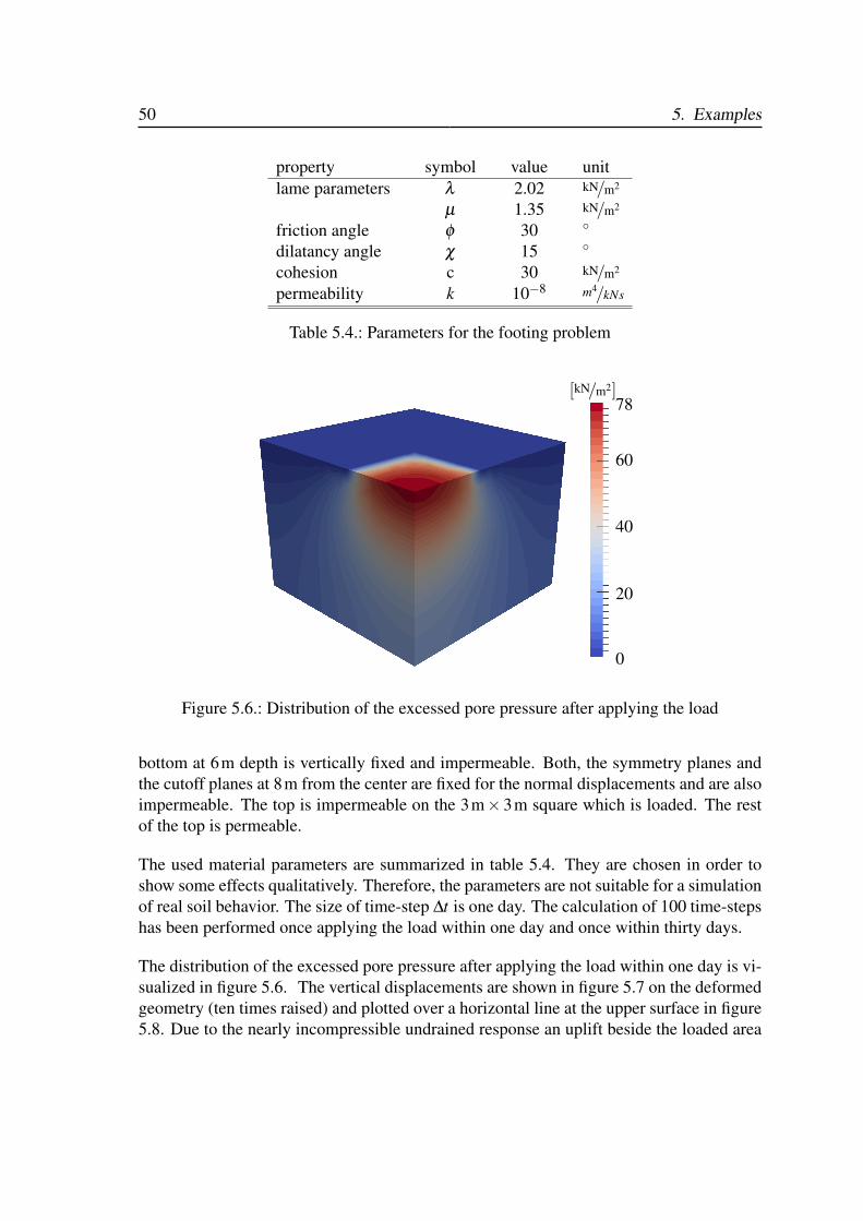
5. EXAMPLES

The solution methods for the presented problems haven been implemented in a computercode. This was done within the framework of the Dune-Project [2, 3, 4, 9]. To verify theimplementation of the plasticity a circular tube undergoing plastic strains is considered.For the validation of the poro-elastic interaction problem a column under vertical loadingis considered. In this test, the material parameters are chosen such that no plastic yieldingoccurs. Finally, the full plastic consolidation process under a footing is studied. For allcalculations a quadratic ansatz for the displacements is used. The pore pressure and theplastic strains are approximated linear.

5.1. Circular tube

As an example for the validation of the implemented code an internally pressurized circulartube as depicted in figure 5.1 is considered. An analytical solution to the plain strainproblem with the perfectly plastic von Mises model is given in [17]. The parameters used

a

b

p

Figure 5.1.: Definition of the circular tube

for the analysis are given in table 5.1. Due to the radial symmetrie of the problem only onequater has been discretized. The mesh for the numerical analysis consists of 1560 elementsand 588 nodes. In case of the associative von Mises model, as it is considered here, theplastic strains are volume preserving. In combination of the simple elements used here, this

45

46 5. Examples

property symbol value unitinner radius a 0.1 mouter radius b 0.2 mYoung modulus E 200000 N/m2

Poisson’s ratio ν 0.3 −yield strength σy 400 N/m2

hardening modulus D 200 N/m2

Table 5.1.: Parameters for the internally pressurized tube

iterationstep 0 1 2 3 4 5

1 0.014131 5.9662e-152 1.1932e-143 0.0072457 0.00015706 4.8816e-06 2.2617e-10 3.3466e-154 0.0080283 0.00031447 1.3031e-05 1.0715e-07 1.8088e-135 0.01226 0.0010036 4.7221e-05 5.0109e-06 4.4616e-10 5.8174e-156 0.0090735 0.00051594 1.081e-05 8.2934e-08 9.357e-147 0.0070128 0.00059659 1.1666e-06 1.5184e-118 0.0054439 0.00051928 3.3568e-06 7.221e-119 0.0044958 0.00023467 1.7651e-06 9.0492e-11

10 0.0036713 0.00046022 1.4525e-05 1.351e-06 5.8372e-1111 0.003625 4.2625e-05 3.4497e-06 5.2422e-10 3.2603e-1112 0.0022817 1.9971e-05 2.6467e-08 1.3233e-1113 0.00015271 2.0042e-08 4.9444e-1414 0.00013202 1.6967e-08 4.4476e-1315 0.0001151 1.38e-08 3.7983e-13

Table 5.2.: Residua of the Newton-like method

leads to wrong solutions if the plastic strains are large in comparison to the elastic strains.Therefor, a small hardening modulus is chosen for the numerical stability. In general withongoing yielding, the number of iterations of the iterative solver increases. Nevertheless,table 5.2 shows the super-linear convergence of the Newton-like method. The obtainedpressure-displacement curve is plotted in figure 5.2. It has a good a agreement with theclosed-form solution.

5.2. Poro-elastic column 47

0 2 ·10−4 4 ·10−4

0

100

200

300

outer displacment u [m]

inte

rnal

pres

sure

p[P

a]

Figure 5.2.: Comparison of the analytic solution and numeric solution

5.2. Poro-elastic column

To verify the solution methods for the poro-elastic interaction within the elastic range, acolumn is considered. An analytical solution to the one dimensional problem with bound-

x = h

x = 0

x

σ = σ0p = 0

u = 0,q = 0

un = 0q = 0

Figure 5.3.: Definition of the column problem

ary conditions as depicted in figure 5.3 is given in [21]. The bottom of the column is fixedand impermeable, the top is loaded with the traction σ0 but the fluid can escape. For thethree dimensional case the walls are also impermeable and fixed horizontally, i.e. in nor-mal direction. Homogeneous initial conditions are assumed. The analytic distribution of

48 5. Examples

property symbol value unitheight h 10 mlame parameters λ 5.56 kN/m2

µ 8.33 kN/m2

permeability k 10−9 m4/Ns

applied load σ0 100 kN/m2

Table 5.3.: Parameters for the column problem

the effective stress

σeff = σ0

(−1+

∞

∑i=0

2M

sin(

Mxh

)e−M2t

), (5.1)

the displacements

u =hσ0

λ +2µ

(1+

∞

∑i=0

2M

sin(

Mxh

)e−M2t

), (5.2)

and the pore pressure

p =∞

∑i=0

2M

sin(

Mxh

)e−M2t , (5.3)

are compared to the results obtained from the tree dimensional analysis. A mesh consistingof 300 elements and 130 nodes has been used. In (5.1), (5.2) and (5.3) the abbreviations

t = (λ +µ)kt,

M =π(2i+1)

2

(5.4)

have been used. In table 5.3 chosen parameters are summarized. The maximum displace-ment occurs on the top of the column. From figure 5.4 and 5.5 a good agreement of thenumerical results and the analytic one dimensional solution can be seen.

5.3. Footing

As a last example a footing problem is considered. The soft ground of 6m height ismodeled with the linear isotropic elasticity model in combination with the non-associativeDrucker-Prager plasticity model. This represents only a rough approximation of real soilbehavior. On a 6m× 6m square a load of 100 kN/m2 is applied within two different timeranges. Any gravity loading is neglected and homogeneous initial conditions are assumed.Due to the symmetry of the problem, only one quarter is simulated. The mesh consistsof 17666 elements and 3718 nodes. The boundary conditions are set as follows. The

5.3. Footing 49

0 1 2 3 4 5·106

0

2 ·10−2

4 ·10−2

time [s]

vert

ical

disp

lacm

ent[

m]

analytic solutionnumerical solution

Figure 5.4.: Displacement at the top of the column plotted over time

0 1 2 3 4 5·106

−100

−50

0

time [s]

vert

ical

effe

ctiv

est

ress

[m]

analytic solutionnumerical solution

Figure 5.5.: Effective stress at the bottom of the column plotted over time

50 5. Examples

property symbol value unitlame parameters λ 2.02 kN/m2

µ 1.35 kN/m2

friction angle φ 30

dilatancy angle χ 15

cohesion c 30 kN/m2

permeability k 10−8 m4/kNs

Table 5.4.: Parameters for the footing problem

0

20

40

60

78[kN/m2]

Figure 5.6.: Distribution of the excessed pore pressure after applying the load

bottom at 6m depth is vertically fixed and impermeable. Both, the symmetry planes andthe cutoff planes at 8m from the center are fixed for the normal displacements and are alsoimpermeable. The top is impermeable on the 3m× 3m square which is loaded. The restof the top is permeable.

The used material parameters are summarized in table 5.4. They are chosen in order toshow some effects qualitatively. Therefore, the parameters are not suitable for a simulationof real soil behavior. The size of time-step ∆t is one day. The calculation of 100 time-stepshas been performed once applying the load within one day and once within thirty days.

The distribution of the excessed pore pressure after applying the load within one day is vi-sualized in figure 5.6. The vertical displacements are shown in figure 5.7 on the deformedgeometry (ten times raised) and plotted over a horizontal line at the upper surface in figure5.8. Due to the nearly incompressible undrained response an uplift beside the loaded area

5.3. Footing 51

−0.075

−0.06

−0.04

−0.02

0.00

0.016[m]

Figure 5.7.: Vertical displacements plotted on the deformed configuration after applyingthe load

happens.

The excessed pore pressure and the vertical displacement at the center of the loading areaare plotted over time in figures 5.9 and 5.10. When applying the load within one day themaximum excessed pore pressure is higher than applying the load within thirty days. Thisis because already some consolidation happens during loading. If the pressure is carriedfrom the water, less stabilizing pressure acts on the solid skeleton. Therefore, the yieldstrength is lower. This explains why some plastic strains occur when loading happenswithin one day. In case of loading within thirty days no plastic reactions occur. Therefore,the final vertical displacements are slightly lower. A qualitative distribution of the plasticstrains is given in figure 5.11.

52 5. Examples

0 2 4 6 8−8

−6

−4

−2

0

2·10−2

distance from center [m]

vert

ical

disp

lacm

ent[

m]

Figure 5.8.: Vertical displacements along a line at the top after applying the load

0 2 4 6 8·106

0

20

40

60

80

time [s]

exce

ssed

pore

pres

sure

[kPa

] one daythirty days

Figure 5.9.: Excessed pore pressure at the center plotted over time

5.3. Footing 53

0 2 4 6 8·106

−0.12

−0.1

−8 ·10−2

−6 ·10−2

−4 ·10−2

−2 ·10−2

0

time [s]

vert

ical

disp

lacm

ent[

m]

one daythirty days

Figure 5.10.: Vertical displacement at the center plotted over time

Figure 5.11.: Qualitative distribution of the plastic strains for loading within one day

54 5. Examples

6. CONCLUSION

In the present work we deal with a theoretical approach to model consolidation phenom-ena and its numerical realization with a finite element method. Thereby, we focused onBiot’s model for a two-phase porous media relaying on an effective stress approach. Aris-ing inertia terms and therefor dynamical effects are neglected from the outset. Both, thesolid grains and the fluid are assumed to be incompressible. The constitutive equationsfor the effective stresses are a linear isotropic elasticity model in combination with a non-associative Drucker-Prager model or an associative von Mises model with linear isotropichardening. The restriction on a linearized geometry description allows an additive split ofthe strain tensor in an elastic and a plastic strain tensor. Additionally to the discretizationof the primal field variables, here the displacement field and the pore pressure field, weintroduced a discretization of the plastic strain field. As the nonlinear problem is solvedwith a Newton-like method, we derived a consistent linearization of the underlying equa-tions and provide closed-form formulas for the tangential stiffness matrix. This leads to asuper-linear convergent method. This was verified in a numerical example. As an open is-sue remains the treatment of the plastic strains on partly plastified elements. As a standardapproach adaptive refinement of the mesh is proposed in the literature. Due to the dis-cretization of the plastic strain field another approach seems fruitful. The plastic responsecould be evaluated in each node whether the yield criterion is violated or not. Then theregion where a plastic response occures could be determined approximately.

Other possible extensions of the presented work are obvious. When taking inertia termsinto account also wave propagation phenomena could be studied. The porous mediumcould be infiltrated by more than one fluid and compressible constitutes could be analyzed.The elasticity model could be extended to account for non-linear and anisotropic behave.Also more complex plasticity models could be used. The consideration of the geometricexact description in combination with a multiplicative decomposition of the deformationgradient in an elastic and a plastic part would be possible.

55

56 6. Conclusion

A. SPACE, FRAMES AND TENSORS

The space of consideration for any physical object in this work is the three-dimensionalEuclidean space E3. No distinction between E3 and R3 is made. With the choice of a fixedspecific reference point in the space, distances can be measured. Any point in the spacecan then be described by three real numbers, its coordinates. These coordinates only makesense in connection with a coordinate system, mapping the numbers to the right point inspace.

Definition 9. (Coordinate system) A coordinate system zi on R3 is a C∞ map of an openset Oz ∈ R3 → R3, whose range is an open set Ox ∈ R3 and the inverse of the Oz → Oxmapping is also a C∞ map.

With definition of a coordinate system also coordinate lines are defined.

Definition 10. (Coordinate lines) The coordinate lines of zi are the curves c1(z1), c2(z2),c3(z3) whose components in the common frame are

for the first coordinate linexi(c1(z1)) = zi(z1,z2,z3) where z2 and z3 are fixed,

for the second coordinate linexi(c2(z2)) = zi(z1,z2,z3) where z1 and z3 are fixed,

and for the third coordinate linexi(c3(z3)) = zi(z1,z2,z3) where z1 and z2 are fixed.

As the reference point and the coordinate system can be chosen arbitrarily, a transformationlaw between the coordinates referring to different coordinate systems is necessary. Theassertion of an Euclidean space implies that there is an rectangular Cartesian coordinatesystem, to which all points refer [31, p. 241]. This common frame is fixed at the beginningbut the choice is not unique as mentioned before. All other frames are derived from thecommon frame. A point r in space is expressed in the common frame through its realcoordinates ri

r = riei = r1e1 + r2e2 + r3e3 (A.1)

where ei is the i-th unit coordinate vector of the common frame.Taking an arbitrarily cho-sen coordinate system za the coordinates of the same point r as in (A.1) are given by

rza = za−1(re

i ), (A.2)

57

58 A. Space, Frames and Tensors

where rei are the coordinates with respect to the common frame.

To describe physical properties explicitly, the reference to base vectors is necessary.

Definition 11. (Coordinate base vectors) Let ei be the base vectors of the common frame,which are independent from the point in space. The tangents to the coordinate lines of acoordinate system za

azb =

∂xi(cb(zb))

∂ zbei b = 1 . . .3, (A.3)

are then the coordinate base vectors of za, which depend in general on the position inspace.

As indicated before, in general one can establish as many coordinate systems (with differ-ent base vectors) as wanted and transfer the representation of the physical quantity to thenew coordinate system. As there are physical properties depending on a different numberof sets of base vectors, the transformation law for each property has to be adjusted to thenumber of sets of base vectors needed. For instance the mass density of a matter is mod-eled with a scalar field which has no dependency on a base vector, the force on a bodyis modeled by a vector with three components which have reference to one set of basevectors. For the generalization of the force concept, the notion of stress is introduced inchapter 2.2. As the quantity describing the stress relates two vectors with each other, it willdepend on two sets of base vectors and will therefore have nine components. In general,such quantities are called tensors.

Consider the quantity Q, which has the components Qi j...kl with n indices i, j...k, l, whichall refer to the base vectors of the same coordinate system zi. Therefore, 3n componentsare needed to describe the quantity. If the coordinate system yi is changed to zα and,therefore, the base vectors (see A, Definition 11) are transformed according to

azα =

∂xk

∂ zα

ek→ ek =∂ zα

∂xkaz

α

ayi =

∂xk

∂yiek→ ay

i =∂xk

∂yi

∂ zα

∂xkaz

α =∂ zα

∂yiaz

α ,

then Q transforms according to

Q = Qi j...klayi ay

j...aykay

l = Qαβ ...γδ

∂ zα

∂yi

∂ zβ

∂y j...

∂ zγ

∂yk

∂ zδ

∂ylaz

αazβ...az

γazδ

(A.4)

and its components transform like

Qyi j...kl = Qz

αβ ...γδ

∂ zα

∂yi

∂ zβ

∂y j...

∂ zγ

∂yk

∂ zδ

∂yl

Qzαβ ...γδ

= Qyi j...kl

∂yi

∂ zα

∂y j

∂ zβ

...∂yk

∂ zγ

∂yl

∂ zδ

.

59

Physical quantities have to be invariant against a change of the coordinate system and,therefore, transform its representation as given above. Because of the dependency on nsets of base vectors Q is called a tensor of order n.

60 A. Space, Frames and Tensors

REFERENCES

[1] ALTENBACH, H. Kontinuumsmechanik: Einführung in die materialunabhängigenund materialabhängigen Gleichungen. Springer, Berlin, 2012.

[2] BASTIAN, P., BLATT, M., DEDNER, A., ENGWER, C., FAHLKE, J., GRÄSER, C.,KLÖFKORN, R., NOLTE, M., OHLBERGER, M., AND SANDER, O. DUNE Webpage, 2011. http://www.dune-project.org.

[3] BASTIAN, P., BLATT, M., DEDNER, A., ENGWER, C., KLÖFKORN, R., KORNHU-BER, R., OHLBERGER, M., AND SANDER, O. A Generic Grid Interface for Paral-lel and Adaptive Scientific Computing. Part II: Implementation and Tests in DUNE.Computing 82, 2–3 (2008), 121–138.

[4] BASTIAN, P., BLATT, M., DEDNER, A., ENGWER, C., KLÖFKORN, R.,OHLBERGER, M., AND SANDER, O. A Generic Grid Interface for Parallel andAdaptive Scientific Computing. Part I: Abstract Framework. Computing 82, 2–3(2008), 103–119.

[5] BIOT, M. A. General theory of three-dimensional consolidation. Journal of AppliedPhysics 12, 2 (1941), 155–164.

[6] BIOT, M. A. Theory of elasticity and consolidation for a porous anisotropic solid.Journal of Applied Physics 26, 2 (1955), 182–185.

[7] BIOT, M. A. Theory of propagation of elastic waves in a fluid-saturated porous solid.I. Low-frequency range. The Journal of the Acoustical Society of America 28 (1956),168–178.

[8] BIOT, M. A. Theory of propagation of elastic waves in a fluid-saturated poroussolid. II. Higher frequency range. The Journal of the Acoustical Society of America28 (1956), 179–191.

[9] BLATT, M., AND BASTIAN, P. The iterative solver template library. In Applied Par-allel Computing. State of the Art in Scientific Computing (Berlin, 2007), B. Kågström,E. Elmroth, J. Dongarra, and J. Wasniewski, Eds., vol. 4699 of Lecture Notes in Com-puter Science, Springer, pp. 666–675.

[10] BOWEN, R. M. Incompressible porous media models by use of the theory of mix-tures. International Journal of Engineering Science 18, 9 (1980), 1129–1148.

61

62 References

[11] BOWEN, R. M. Compressible porous media models by use of the theory of mixtures.International Journal of Engineering Science 20, 6 (1982), 697–735.

[12] BRAESS, D. Finite Elemente: Theorie, schnelle Löser und Anwendungen in derElastizitätstheorie. Springer, London, 2007.

[13] COUSSY, O. Mechanics of porous continua. John Wiley and Sons Ltd., Chichester,1995.

[14] DE BOER, R. Theory of porous media - past and present. ZAMM - Journal of AppliedMathematics and Mechanics 78, 7 (1998), 441–466.

[15] DE SOUZA NETO, E., PETRIC, D., AND OWEN, D. Computational Methods forPlasticity. John Wiley and Sons Ltd., Chichester, 2008.

[16] GREVE, R. Kontinuumsmechanik. Springer, Berlin, 2003.

[17] HILL, R. The mathematical theory of plasticity. Oxford University Press, New York,1950.

[18] JUNG, M., AND LANGER, U. Methode der finiten Elemente für Ingenieure. Springer,Berlin, 2001.

[19] LEWIS, R. W., AND SCHREFLER, B. A. The finite element method in the defor-mation and consolidation of porous media. John Wiley and Sons Inc., New York,1987.

[20] MARSDEN, J. E., AND HUGHES, T. J. Mathematical foundations of elasticity.Dover Publications, New York, 1983.

[21] MURAD, M. A., AND LOULA, A. F. Improved accuracy in finite element analy-sis of Biot’s consolidation problem. Computer Methods in Applied Mechanics andEngineering 95, 3 (1992), 359 – 382.

[22] ORTIZ, M., AND POPOV, E. P. Accuracy and stability of integration algorithms forelastoplastic constitutive relations. International Journal for Numerical Methods inEngineering 21, 9 (1985), 1561–1576.

[23] PETER, G., KIENESBERGER, J., LANGER, U., SCHÖBERL, J., AND VALDMAN,J. Fast solvers and a posteriori error estimates in elastoplasticity. In Numerical andSymbolic Scientific Computing. Springer, 2012, pp. 45–63.

[24] SAUTER, M., AND WIENERS, C. On the superlinear convergence in computationalelasto-plasticity. Computer Methods in Applied Mechanics and Engineering 200, 49(2011), 3646–3658.

[25] SCHANZ, M. Poroelastodynamics: Linear models, analytical solutions, and numeri-cal methods. Applied Mechanics Reviews 62, 3 (2009), 1–15.

References 63

[26] SCHANZ, M., AND DIEBELS, S. A comparative study of Biot’s theory and thelinear theory of porous media for wave propagation problems. Acta Mechanica 161,3-4 (2003), 213–235.

[27] SELVADURAI, P. The analytical method in geomechanics. Applied Mechanics Re-views 60 (2007), 87–106.

[28] SIMO, J., AND HUGHES, T. Computational Inelasticity. Springer, New York, 1998.

[29] SIMO, J. C., AND TAYLOR, R. L. Consistent tangent operators for rate-independentelastoplasticity. Computer methods in applied mechanics and engineering 48, 1(1985), 101–118.

[30] TRUESDELL, C., AND NOLL, W. The non-linear field theories of mechanics inHandbuch der Physik, Vol III, Part 3, edited by S. Flügge. Springer, Berlin, 1965.

[31] TRUESDELL, C., AND TOUPIN, R. The classical field theories in Handbuch derPhysik, Vol III, Part 1, edited by S. Flügge. Springer, Berlin, 1960.

[32] VON TERZAGHI, K. Die Berechnung der Durchlässigkeit des Tones aus dem Verlaufder hydromechanischen Spannungserscheinungen. Sitzungsbericht der Akademie derWissenschaften (Wien): Mathematisch-Naturwissenschaftlichen Klasse 132 (1923),125–138.

[33] WIENERS, C., AMMANN, M., DIEBELS, S., AND EHLERS, W. Parallel 3-d simu-lations for porous media models in soil mechanics. Computational mechanics 29, 1(2002), 75–87.

[34] WILKINS, M. L. Calculation of elastic-plastic flow. Methods of ComputationalPhysics 3 (1963).

[35] WILMANSKI, K. Porous media at finite strains. the new model with the balanceequation for porosity. Archives of Mechanics 48, 4 (1996), 591–628.

[36] WILMANSKI, K. Thermomechanics of continua. Springer, Berlin, 1998.

[37] WRIGGERS, P. Nichtlineare Finite-Element-Methoden. Springer, Berlin, 2001.

[38] YU, H.-S. Plasticity and Geotechnics, vol. 13. Springer, 2006.

[39] ZIENKIEWICZ, O. C., AND TAYLOR, R. L. The finite element method for solid andstructural mechanics. Butterworth-Heinemann, 2005.

Date post:	23-Feb-2022
Category:	Documents
Upload:	others
View:	4 times
Download:	0 times

Finite Element Formulation for the Consolidation Process ...

Documents