Finite Volume simulation of cavitating flows

Thomas Barberon, Philippe Helluy

ISITV, Laboratoire MNC, BP 56, 83162 La Valette, France

Abstract

We propose a numerical method adapted to the modelling of phase transitions incompressible fluid flows. Pressure laws taking into account phase transitions arecomplex and lead to difficulties such as the non-uniqueness of entropy solutions. Inorder to avoid these difficulties, we propose a projection finite volume scheme. Thisscheme is based on a Riemann solver with a simpler pressure law and an entropymaximization procedure that enables us to recover the original complex pressurelaw. Several numerical experiments are presented that validate this approach.

Key words: cavitation, Godunov scheme, two-phase compressible flow

1 Introduction

This work is devoted to the numerical modelling of phase transition in com-pressible fluid flows. We focus on the liquid-vapor phase transition also calledcavitation. For this we consider the Euler system for an inviscid and com-pressible fluid together with a pressure law that ensures the hyperbolicity ofthe Euler system. This system has been extensively studied, both theoreticallyand numerically. Standard textbooks exist now on this subject [13], [27], [28].The global existence and uniqueness of a solution to this system, for generalinitial conditions, is still an open question.

On the other hand, the Riemann problem, which consists of finding a onedimensional solution for a particular initial condition made of two constantstates, is well understood. It is known that a supplementary dissipation cri-terion must be added in order to recover uniqueness. This criterion can takeseveral forms. The most classical criteria are:

(1) The Lax entropy criterion: any Lax entropy should increase in shocks.

Email address: helluy@univ-tln.fr (Philippe Helluy).

Preprint submitted to Elsevier Science 6 April 2004

(2) The Lax characteristic criterion: a shock of the i−th family should becrossed by the i−th characteristics coming from the two sides of theshock.

(3) The vanishing viscosity criterion: the solution should be the limit of solu-tions of the Euler system perturbed by a supplementary viscosity term.

(4) Liu has proposed in [21] a stricter criterion than the Lax entropy criterion(1). It requires that the entropy increases along the entire shock curvejoining the left and the right states of the shock and not only globally.

In the case of a simple pressure law, such as the perfect gas law, it appearsthat these four criteria are equivalent and ensure existence and uniquenessof the solution. But for more complex laws used for the modelling of phasetransitions, the situation is not so clear. In some configurations, one can indeedfind several solutions satisfying criteria (1)-(4), even if the pressure law ensuresthe hyperbolicity of the system. A very detailed study of these topics can befound in the important paper of Menikoff and Plohr [22]. Detailed examplescan also be found in the thesis of Jaouen [16]. In this reference a proof of non-uniqueness is also given in the case of a simplified phase transition pressurelaw.

It can also happen that none of the criteria (2)-(4) are physically relevant. Forinstance, Hayes and LeFloch study in [14] the effect of a vanishing third orderperturbation to the initial hyperbolic system. This term permits to modelcapillarity near the critical point. They show that in general the limit shocksolutions do not satisfy criteria 2-4. Special schemes have to be designed inorder to approximate these non-classical shocks [19].

For classical pressure laws, the Riemann problem solution is made up of sev-eral constant states separated by shock waves, simple waves and one contactdiscontinuity. Phase transition pressure laws may present pathologies such asslope discontinuities, lack of convexity of the isentropes or of the Hugoniotcurves in the (τ, p) plane. These pathologies lead to a more complex resolu-tion of the Riemann problem. One has to take into account the possibility ofcomposite waves. This subject is studied in the paper of Menikoff and Plohr[22]. Classical references about the Riemann problem for arbitrary fluids arealso [5], [31], [30]. Thus, even if the Riemann problem is still uniquely solvable,it is difficult to practically implement it in a Godunov type scheme.

Several numerical methods have been proposed to solve the Euler system withcomplex pressure laws. Some methods rely on approximate Riemann solvers[12], [16], [2]. These methods must be carefully employed because even if thescheme is entropic it may converge towards wrong solutions due to the non-uniqueness of the solution. This possible behavior is illustrated in [16], wherean entropic Godunov-type scheme converges to different solutions accordingto the CFL number.

2

In this paper we focus on special pressure laws. We suppose that the pressurelaw is obtained from a physical entropy maximization with respect to supple-mentary (intermediate) variables. This is not a restriction for phase transitionsbecause it is exactly the way the liquid-vapor mixture is classically modelled[6]. We then use this representation in order to design a finite volume scheme,which we first described in [15] and [3]. Each time-step of this scheme is madeup of two sub-steps:

(1) A standard Godunov resolution taking into account the intermediate vari-ables. In this step, the intermediate variables are simply convected withthe fluid. It appears that the associated Riemann problem is easier tosolve than the original one. Indeed, the relaxed pressure law with inter-mediate variables has no pathology. This step is entropic because we usean exact Riemann solver.

(2) Then, the conservative variables are kept for the next time step. Thepressure is updated by maximizing the physical entropy with respectto the intermediate variables. This amounts to projecting the relaxedpressure law towards the real pressure law. This step is also entropic byconstruction.

The paper is thus organized as follows.

Following this Introduction, the second section is devoted to a presentation ofa simple mathematical framework for the modelling of phase transition. Weconsider the flow of a compressible liquid which is subject to phase transition.The idea is to add to the initial Euler system a convection equation with arelaxation source term for a supplementary vector Y (t, x) called the fractionsvector, which plays the role of the intermediate variables. The complex initialpressure law is replaced by a simpler relaxed pressure law which depends ondensity, internal energy and the fractions. We associate an entropy to thissimpler pressure law. We then define the equilibrium fractions Yeq by an op-timization of the entropy with respect to Y . We suppose that the complexpressure law is recovered by replacing Y with Yeq in the relaxed pressure law.

The idea of replacing a complex pressure law by a simpler one together with arelaxation procedure was first proposed by Coquel and Perthame in [9]. Relax-ation source terms are extensively used in the seven-equation model of Abgralland Saurel in [24]. This idea has also been exploited in [7], [18] for the mod-elling of two-phase flows without phase transition. Even when the two phasesare supposed to be immiscible, it is necessary, for numerical reasons, to definea mixture pressure law. This mixture pressure law is obtained by imposingpressure equilibrium between the two phases and can be quite complicated.Thus, in order to use an exact Riemann solver, it is interesting to relax thepressure law. This is done in [7], [18] by solving a supplementary convectionequation for the volume fraction of one fluid. At the end of each time step,

3

this volume fraction is modified in order to recover the pressure equilibrium.

We then apply the above mathematical framework to a physical model ofvapor-liquid mixture. We consider two fluids which are supposed to be immis-cible on a small scale. The behavior of each fluid is entirely described by itsspecific entropy which is a function of the specific volume and of the internalenergy. Using the physical fact that the entropy is an extensive variable, it isthen possible to get in a unique manner the mixture entropy, function of thespecific volume, the internal energy and the fractions. Then the second prin-ciple of thermodynamics tells us that the equilibrium fractions must realizea maximum of the mixture entropy. This maximization process enables us toreconstruct a physically coherent equilibrium pressure law.

In the third section of the paper, we apply this theory to a mixture of twophases satisfying the stiffened gas equation of state. In order to have simplercomputations, we suppose that thermal equilibrium always hold. In this way,it is possible to eliminate the energy fraction from the unknowns. Then, animportant feature is that the resulting relaxed mixture pressure law is still astiffened gas law even though the equilibrium pressure law is no longer one. Ifthe stiffened gases are perfect gases, the computations are even simpler.

The fourth section is devoted to the study of the Riemann problem associ-ated to the pressure law of the previous section. We briefly explain how it ispossible to construct several entropy solutions to the Riemann problem. Thisconstruction is not original and is entirely contained in the thesis of Jaouen[16]. It is used in the fifth section to validate the numerical scheme.

In the fifth section, we present the projection scheme. The description is verysimple. Each time step of the finite volume scheme is made up of two stages.In the first stage, a simple Godunov scheme is employed. Thus, in this stage,the phase transition is not taken into account. Because the pressure law issimplified, it is possible to use an exact Riemann solver and to have the correctentropy dissipation. In the second stage, the fraction vector is modified in sucha way as to maximize the entropy of the mixture in each cell. This stage isconservative, because the density, velocity and energy are not modified. It isalso entropy dissipative by construction.

We then illustrate the projection scheme on several 1D numerical experiments.In particular, we verify that it is able to reproduce the physical entropy solutionconstructed in Section 4. It is important to notice here that the numericalsolution does not depend on the CFL number. We explain the good behaviorof the projection scheme by the fact that the production of entropy occursnot only in the Godunov step but also because of the phase transition. Thisis important because a global entropy production is not sufficient.

Section 6 is then devoted to a 2D simulation in order to illustrate the ability

4

of our scheme to deal with physical configurations. This test is very similar tothe one proposed by Butler, Cocchi and Saurel in [26]. The goal is to computethe flow around a fast projectile diving into water at a velocity of 1000 m/s.A strong pressure loss appears in the wake of the projectile, triggering thegrowth of a cavitation pocket. We are able to qualitatively reproduce thisphenomenon.

The paper ends with a conclusion (Section 7).

2 Mathematical models for phase transition

This section is devoted to a presentation of a simple mathematical frameworkfor the modelling of phase transition. We consider the two-phase vapor-liquidmixture as a single compressible medium with (in 1D) density ρ(t, x), velocityu(t, x), internal energy ε(t, x) and pressure p(t, x), all depending on the timevariable t and the space variable x. Conservation of mass, momentum andenergy and Newton’s law for inviscid flow lead to the three Euler equations:

ρt + (ρu)x = 0,

(ρu)t + (ρu2 + p)x = 0, (1)

(ρε + ρu2/2)t + ((ρε + ρu2/2 + p)u)x = 0.

If the flow is not too fast, i.e. if the equilibrium between the liquid and itsvapor is achieved for all (t, x), the pressure of the whole mixture depends onlyon the density ρ and the internal energy ε. We shall write

p = peq(ρ, ε). (2)

This equilibrium pressure law is generally quite complex, and more important,leads to unclassical behaviors of the solutions: non-uniqueness of the entropysolution, composite waves. We insist on the fact that this has nothing to dowith a defect of hyperbolicity. Phase transition pressure laws naturally ensurethe hyperbolicity. For example, the Van der Waals pressure law is a bad modelof phase transition and has to be modified by Maxwell’s construction in orderto eliminate the elliptic region, and the modified law ensures hyperbolicity [6].

We propose in this section a more general model, in which we no longer sup-pose the equilibrium of the two-phase mixture. We have thus to introducesupplementary variables and the pressure will also depend on these variables.This pressure law will be called the relaxed pressure law. Because the resultingmodel is out of equilibrium, we shall denote it as the metastable model.

5

Of course we will also have to return to the equilibrium pressure law. This willbe done by a projection method. Although it would be interesting to accountfor the dynamics of the phase transition, we do not deal with this problemhere and just use the metastable model in order to compute the equilibriummodel.

2.1 A generalized metastable model

A supplementary vector of variables, called the fractions vector Y (t, x) is usedin order to model vaporization. The components Y i, 1 ≤ i ≤ N satisfy

0 ≤ Y i ≤ 1. (3)

Usually, the fraction vector Y will have three components that are the mass,volume and energy fractions of the vapor in the mixture. But simpler modelswill only consider one or two fractions. We suppose that when the fluid is pureliquid, Y i = 0, and when the fluid is pure vapor, Y i = 1. When no phasetransition occurs, there is no transfer between the liquid and its vapor, thuswe also have perfect convection of the fractions:

Yt + uYx = 0. (4)

Using the mass conservation law, the convection of the fractions can be writtenin an equivalent conservative form

(ρY )t + (ρuY )x = 0. (5)

We have to close these equations with a pressure law

p = p(ρ, ε, Y ). (6)

When equations (1), (5) and (6) are considered, we will speak of the metastablemodel. Indeed, in this model the fractions are simply convected in the flow,and thus, there is no transfer between the two phases.

It is well known that the solution of model (1), (5), (6) is not unique and thata supplementary condition has to be added to restrict the set of solutions.For a simple pressure law, this can be an entropy growth criterion. But it canbe necessary to envisage other criteria as described in the Introduction. Withτ = 1/ρ, an entropy is a concave function s = s(τ, ε, Y ), solution of the firstorder PDE

sτ − p(1/τ, ε, Y )sε = 0. (7)

Generally, one can find several entropies. Defining the temperature by

T = 1/sε, (8)

6

we recover the relation

Tds = dε + pdτ + sY dY. (9)

Thus, choosing an entropy amounts to choosing the temperature scale. It alsopermits us to recover the pressure law by

p = Tsτ . (10)

A given entropy is called a complete equation of state (see [22]) because itpermits us to recover the pressure law (10) and the caloric law (8). When onestudies the dynamic behavior of a compressible fluid, an incomplete equationof state, the pressure law, is sufficient. But if one wishes to model a ther-modynamic feature such as the phase transition, it is necessary to fix thetemperature scale and thus a complete equation of state is required. In thesequel, we then suppose that one particular entropy has been selected. Theconstruction of the mixture entropy from the entropies of the two phases andfrom physical considerations is described below.

Simple computations show that a regular solution of system (1), (5), (6) sa-tisfies

st + usx = 0, (11)

which can be cast into a conservative form

(ρs)t + (ρus)x = 0. (12)

When dealing with discontinuous solutions, the latter has to be replaced byan inequality, in the sense of distributions, in order to recover uniqueness

(ρs)t + (ρus)x ≥ 0. (13)

Recall that the concavity of s with respect to (τ, ε, Y ) is equivalent to theconvexity of the quantity U = −ρs with respect to the conservative variables(ρ, ρu, ρε + ρu2/2, ρY ) (see [13], [10]). This implies that U = −ρs is indeed aLax entropy of the metastable model.

2.2 Entropy compatible transition models

In order to take phase transition into account, we add a source term to equation(5)

Yt + uYx = µ. (14)

Equations (1), (6) together with (14) will be referred to as the cavitation ortransition model. In the case where the phase transition is infinitely fast, wewill always have

Y = Yeq(ρ, ε), (15)

7

because the repartition of liquid and vapor is completely determined by thephase diagram. We require that the resulting pressure law is exactly the equi-librium pressure law (2)

p = p(ρ, ε, Yeq(ρ, ε)) = peq(ρ, ε). (16)

It is then natural to consider, as in [9], a relaxation source term of the form

µ = λ(Yeq(ρ, ε)− Y ), (17)

and then to let λ →∞.

Suppose then that the equilibrium fractions Yeq are defined by

s(ρ, ε, Yeq(ρ, ε)) = maxY ∈Q

s(ρ, ε, Y ), (18)

where Q is the set of admissible parameters.

It is then interesting to compute the production of entropy along the stream-lines of the flow, when all the unknowns are regular. Using (10) and (8), thisproduction is given by

s := st + usx = sτ (τt + uτx) + sε(εt + uεx) +∇Y s · (Yt + uYx)

=−p

Tρ2(ρt + uρx) +

1

T(εt + uεx) +∇Y s · (Yt + uYx).

(19)

But on the other hand, a regular solution of the Euler system (1) also satisfies

ρt + uρx + ρux = 0,

ut + uux +px

ρ= 0,

εt + uεx +p

ρux = 0,

(20)

thus, the production of entropy can be simplified and thanks to the concavityof s, for the cavitation model (equations (1), (6), (14) and (17)) we have also

st + usx = ∇Y s · (Yt + uYx) ,

= λ∇Y s · (Yeq − Y )

≥ λ (s(Yeq)− s(Y ))

≥ 0,

(21)

The entropy condition is thus reinforced when compared to the metastablemodel (equations (1), (5) and (6)) because the production of entropy occursnot only in shocks but also as a result of the phase transition.

8

2.3 Mixture entropy

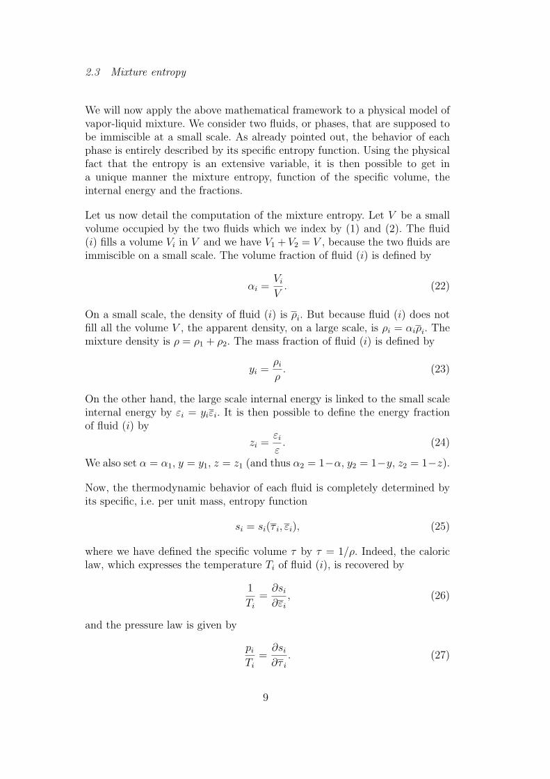
We will now apply the above mathematical framework to a physical model ofvapor-liquid mixture. We consider two fluids, or phases, that are supposed tobe immiscible at a small scale. As already pointed out, the behavior of eachphase is entirely described by its specific entropy function. Using the physicalfact that the entropy is an extensive variable, it is then possible to get ina unique manner the mixture entropy, function of the specific volume, theinternal energy and the fractions.

Let us now detail the computation of the mixture entropy. Let V be a smallvolume occupied by the two fluids which we index by (1) and (2). The fluid(i) fills a volume Vi in V and we have V1 + V2 = V , because the two fluids areimmiscible on a small scale. The volume fraction of fluid (i) is defined by

αi =Vi

V. (22)

On a small scale, the density of fluid (i) is ρi. But because fluid (i) does notfill all the volume V , the apparent density, on a large scale, is ρi = αiρi. Themixture density is ρ = ρ1 + ρ2. The mass fraction of fluid (i) is defined by

yi =ρi

ρ. (23)

On the other hand, the large scale internal energy is linked to the small scaleinternal energy by εi = yiεi. It is then possible to define the energy fractionof fluid (i) by

zi =εi

ε. (24)

We also set α = α1, y = y1, z = z1 (and thus α2 = 1−α, y2 = 1−y, z2 = 1−z).

Now, the thermodynamic behavior of each fluid is completely determined byits specific, i.e. per unit mass, entropy function

si = si(τ i, εi), (25)

where we have defined the specific volume τ by τ = 1/ρ. Indeed, the caloriclaw, which expresses the temperature Ti of fluid (i), is recovered by

1

Ti

=∂si

∂εi

, (26)

and the pressure law is given by

pi

Ti

=∂si

∂τ i

. (27)

9

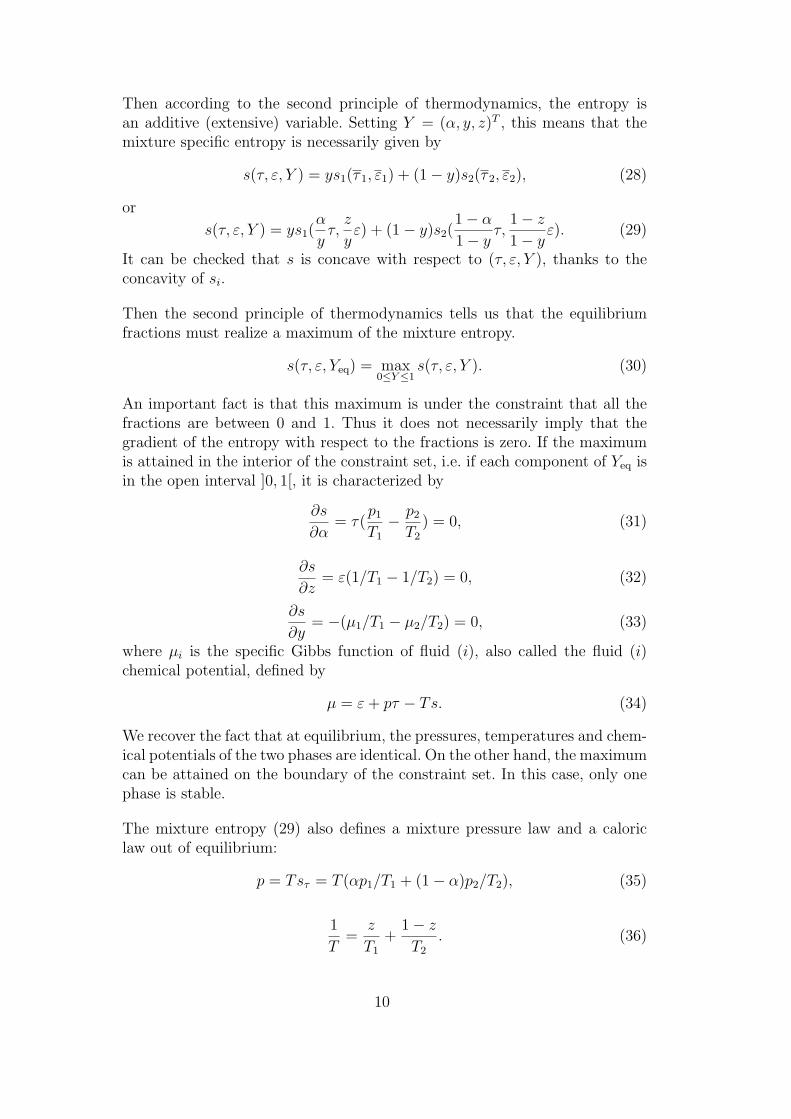
Then according to the second principle of thermodynamics, the entropy isan additive (extensive) variable. Setting Y = (α, y, z)T , this means that themixture specific entropy is necessarily given by

s(τ, ε, Y ) = ys1(τ 1, ε1) + (1− y)s2(τ 2, ε2), (28)

or

s(τ, ε, Y ) = ys1(α

yτ,

z

yε) + (1− y)s2(

1− α

1− yτ,

1− z

1− yε). (29)

It can be checked that s is concave with respect to (τ, ε, Y ), thanks to theconcavity of si.

Then the second principle of thermodynamics tells us that the equilibriumfractions must realize a maximum of the mixture entropy.

s(τ, ε, Yeq) = max0≤Y≤1

s(τ, ε, Y ). (30)

An important fact is that this maximum is under the constraint that all thefractions are between 0 and 1. Thus it does not necessarily imply that thegradient of the entropy with respect to the fractions is zero. If the maximumis attained in the interior of the constraint set, i.e. if each component of Yeq isin the open interval ]0, 1[, it is characterized by

∂s

∂α= τ(

p1

T1

− p2

T2

) = 0, (31)

∂s

∂z= ε(1/T1 − 1/T2) = 0, (32)

∂s

∂y= −(µ1/T1 − µ2/T2) = 0, (33)

where µi is the specific Gibbs function of fluid (i), also called the fluid (i)chemical potential, defined by

µ = ε + pτ − Ts. (34)

We recover the fact that at equilibrium, the pressures, temperatures and chem-ical potentials of the two phases are identical. On the other hand, the maximumcan be attained on the boundary of the constraint set. In this case, only onephase is stable.

The mixture entropy (29) also defines a mixture pressure law and a caloriclaw out of equilibrium:

p = Tsτ = T (αp1/T1 + (1− α)p2/T2), (35)

1

T=

z

T1

+1− z

T2

. (36)

10

3 A simple pressure law for phase transition

3.1 Mixtures of stiffened gases

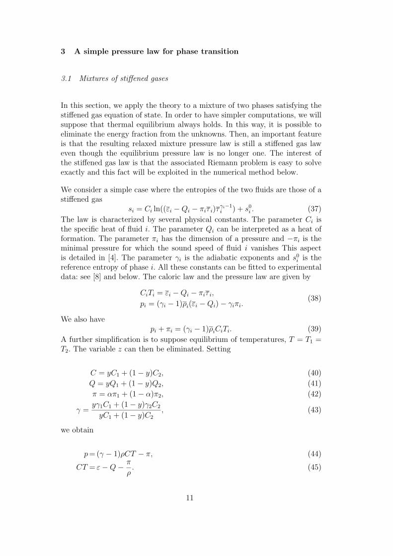
In this section, we apply the theory to a mixture of two phases satisfying thestiffened gas equation of state. In order to have simpler computations, we willsuppose that thermal equilibrium always holds. In this way, it is possible toeliminate the energy fraction from the unknowns. Then, an important featureis that the resulting relaxed mixture pressure law is still a stiffened gas laweven though the equilibrium pressure law is no longer one. The interest ofthe stiffened gas law is that the associated Riemann problem is easy to solveexactly and this fact will be exploited in the numerical method below.

We consider a simple case where the entropies of the two fluids are those of astiffened gas

si = Ci ln((εi −Qi − πiτ i)τγi−1i ) + s0

i . (37)

The law is characterized by several physical constants. The parameter Ci isthe specific heat of fluid i. The parameter Qi can be interpreted as a heat offormation. The parameter πi has the dimension of a pressure and −πi is theminimal pressure for which the sound speed of fluid i vanishes This aspectis detailed in [4]. The parameter γi is the adiabatic exponents and s0

i is thereference entropy of phase i. All these constants can be fitted to experimentaldata: see [8] and below. The caloric law and the pressure law are given by

CiTi = εi −Qi − πiτ i,

pi = (γi − 1)ρi(εi −Qi)− γiπi.(38)

We also havepi + πi = (γi − 1)ρiCiTi. (39)

A further simplification is to suppose equilibrium of temperatures, T = T1 =T2. The variable z can then be eliminated. Setting

C = yC1 + (1− y)C2, (40)

Q = yQ1 + (1− y)Q2, (41)

π = απ1 + (1− α)π2, (42)

γ =yγ1C1 + (1− y)γ2C2

yC1 + (1− y)C2

, (43)

we obtain

p = (γ − 1)ρCT − π, (44)

CT = ε−Q− π

ρ. (45)

11

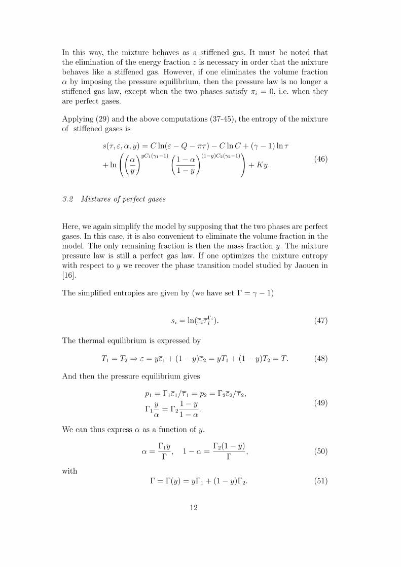
In this way, the mixture behaves as a stiffened gas. It must be noted thatthe elimination of the energy fraction z is necessary in order that the mixturebehaves like a stiffened gas. However, if one eliminates the volume fractionα by imposing the pressure equilibrium, then the pressure law is no longer astiffened gas law, except when the two phases satisfy πi = 0, i.e. when theyare perfect gases.

Applying (29) and the above computations (37-45), the entropy of the mixtureof stiffened gases is

s(τ, ε, α, y) = C ln(ε−Q− πτ)− C ln C + (γ − 1) ln τ

+ ln

(α

y

)yC1(γ1−1) (1− α

1− y

)(1−y)C2(γ2−1) + Ky.

(46)

3.2 Mixtures of perfect gases

Here, we again simplify the model by supposing that the two phases are perfectgases. In this case, it is also convenient to eliminate the volume fraction in themodel. The only remaining fraction is then the mass fraction y. The mixturepressure law is still a perfect gas law. If one optimizes the mixture entropywith respect to y we recover the phase transition model studied by Jaouen in[16].

The simplified entropies are given by (we have set Γ = γ − 1)

si = ln(εiτΓii ). (47)

The thermal equilibrium is expressed by

T1 = T2 ⇒ ε = yε1 + (1− y)ε2 = yT1 + (1− y)T2 = T. (48)

And then the pressure equilibrium gives

p1 = Γ1ε1/τ 1 = p2 = Γ2ε2/τ 2,

Γ1y

α= Γ2

1− y

1− α.

(49)

We can thus express α as a function of y.

α =Γ1y

Γ, 1− α =

Γ2(1− y)

Γ, (50)

withΓ = Γ(y) = yΓ1 + (1− y)Γ2. (51)

12

Finally, again using (29) the mixture entropy is

s = y ln

(ε

(Γ1

Γτ)Γ1

)+ (1− y) ln

(ε

(Γ2

Γτ)Γ2

),

= ln ε + Γ ln τ + yΓ1 ln Γ1 + (1− y)Γ2 ln Γ2 − Γ ln Γ.

(52)

The fraction vector Y is in this case reduced to the mass fraction y. Out ofequilibrium, the mixture is still a perfect gas for we have ∂s

∂ε= 1

T= 1

εand

∂s∂τ

= pT

= Γ(y)τ

.

In the sequel, we suppose that Γ1 > Γ2, i.e. the phase (1) is less dense thanthe phase (2)). The derivative of s with respect to y is

∂s

∂y= (Γ1 − Γ2) ln τ + Γ1 ln Γ1 − Γ2 ln Γ2

−(Γ1 − Γ2) ln Γ− (Γ1 − Γ2).(53)

The saturation curve for this phase transition model is defined by ∂s/∂y = 0.We find that the saturation curve is, in the plane (T, p), a straight line withequation

T

p= exp(1) ln

(ΓΓ2

2

ΓΓ11

) 1Γ1−Γ2

= G. (54)

Maximizing s with respect to y under the constraints 0 ≤ y ≤ 1 permits torecover the equilibrium pressure law

peq(τ, ε) = Γ2ε/τ if τ ≤ τ2,

peq(τ, ε) = Gε if τ2 ≤ τ ≤ τ1,

peq(τ, ε) = Γ1ε/τ if τ ≥ τ1,

(55)

withτi = GΓi. (56)

This model is exactly the one proposed by Jaouen in [16].

4 Construction of an analytical solution

In this part, we consider the Euler system (1) and the pressure law (55). TheEuler system can also be written

Wt + F (W )x = 0, (57)

with W = (ρ, ρu, ρε + ρu2/2)T . We will also use a privileged set of non-conservative variables that we denote V = (τ, u, p)T . We recall briefly how

13

it is possible to construct several entropy solutions to the Riemann problemthat consists of finding solutions to (1) when the initial condition is

W (0, x) =

Wl if x < 0,

Wr if x > 0.(58)

We will compute precisely the correct entropy solution, that is the limit ofviscosity solutions or that satisfies the Liu entropy condition. This analyticalsolution will be used to validate our scheme in Section 5.3.

4.1 A simple entropy shock solution

We only consider solutions made of one or several shock waves. A shock solu-tion of velocity σ has the form

W (t, x) =

WL if x/t < σ,

WR if x/t > σ.(59)

The Rankine-Hugoniot shock conditions must be satisfied. Denoting [φ] thejump of the quantity φ across the discontinuity ([φ] = φR − φL), they can bewritten as σ[W ] = [F (W )] or

σ [ρ] = [ρu] ,

σ [ρu] =[ρu2 + p

],

σ

[ρε + ρ

u2

2

]=

[(ρε + ρ

u2

2+ p

)u

].

(60)

Defining the Lagrangian velocity of the shock by

j = ρL(σ − uL) = ρR(σ − uR), (61)

we have equivalently

j2 = − [p]

[τ ],

j =[p]

[u],

[ε] +1

2[τ ] (pL + pR) = 0.

(62)

If j > 0, we are in the case of a 3-shock, if j < 0, it is a 1-shock. The casej = 0 corresponds to a contact discontinuity. If VR = (τR, uR, pR) is fixed andif j > 0, the three equations in (62) define a curve, called the Hugoniot curve,

14

LLLE

EE

τ

p

τ2 τ1

(τR,pR)

(τ1,p1)

(1)+(2)

(1)

(2)

”gas”

”liquid” saturationzone

o

Rayleighline

(τ ,p)o o

o o

u

p

oo

o

(uR,pR)

(uL,pL)

(u∗,p∗)

1-shock locus oforigin wR

3-shock locus oforigin wL

1-shock locus oforigin w1

o(u,p)

Rayleigh line

(u1,p1)

(τL,pL)

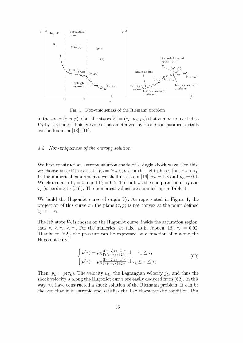
Fig. 1. Non-uniqueness of the Riemann problem

in the space (τ, u, p) of all the states VL = (τL, uL, pL) that can be connected toVR by a 3-shock. This curve can parameterized by τ or j for instance: detailscan be found in [13], [16].

4.2 Non-uniqueness of the entropy solution

We first construct an entropy solution made of a single shock wave. For this,we choose an arbitrary state VR = (τR, 0, pR) in the light phase, thus τR > τ1.In the numerical experiments, we shall use, as in [16], τR = 1.3 and pR = 0.1.We choose also Γ1 = 0.6 and Γ2 = 0.5. This allows the computation of τ1 andτ2 (according to (56)). The numerical values are summed up in Table 1.

We build the Hugoniot curve of origin VR. As represented in Figure 1, theprojection of this curve on the plane (τ, p) is not convex at the point definedby τ = τ1.

The left state VL is chosen on the Hugoniot curve, inside the saturation region,thus τ2 < τL < τ1. For the numerics, we take, as in Jaouen [16], τL = 0.92.Thanks to (62), the pressure can be expressed as a function of τ along theHugoniot curve

p(τ) = pR(Γ1+2)τR−Γ1τΓ1(τ−τR)+2Γ1

if τ1 ≤ τ,

p(τ) = pR(Γ1+2)τR−Γ1τΓ1(τ−τR)+2τ1

if τ2 ≤ τ ≤ τ1.(63)

Then, pL = p(τL). The velocity uL, the Lagrangian velocity jL, and thus theshock velocity σ along the Hugoniot curve are easily deduced from (62). In thisway, we have constructed a shock solution of the Riemann problem. It can bechecked that it is entropic and satisfies the Lax characteristic condition. But

15

this solution is not physical, i.e. has no viscous profile. Details can be found in[16]. We just mention that along the Hugoniot curve, the variation of entropyis given by

Tds =1

2[τ ]2 d

(j2

). (64)

According to (62), j2 is also the opposite of the slope of the Rayleigh line,which is the line joining wR and w) in the plane (τ, p). It can then be seenon Figure 1, that the entropy is increasing between wR and w1 and decreasingbetween w1 and w. The production of entropy in the first part of the Hugoniotcurve is bigger than the decrease of the entropy in the second part. Thus theshock is globally entropic but does not satisfy the Liu entropy condition.

It is indeed possible to construct another solution, which is the only physicalsolution. We keep the first part of the Hugoniot curve, outside the saturationregion. The intersection of the Hugoniot curve and the plane τ = τ1 providesus with a first state V1 = (τ1, u1, p1) and a shock velocity σ1. Then, a Riemannproblem is solved inside the saturation region

Wt + F (W )x = 0,

W (0, x) =

WL if x < 0,

W1 if x > 0.

(65)

This Riemann problem has only one entropy solution, because inside the sa-turation region, the pressure law presents no pathology. Details are given in[16]. The Liu solution thus has the form

V (t, x) =

VL if x/t < σL,

Vm,L if σL < x/t < um,

Vm,1 if um < x/t < σm,1,

V1 if σm,1 < x/t < σ1,

VR if σ1 < x/t,

(66)

withVm,L = (τm,L, um, pm),

Vm,1 = (τm,1, um, pm).(67)

Recall that, because only shock solutions occur, we have to find the intersectionof the 1-shock locus of origin (u1, p1) and the 3-shock locus of origin (uL, pL).Thanks to (62), one has

τm,L(pm) = τL + 2pL − pm

G(pm + pL),

τm,1(pm) = τ1 + 2p1 − pm

G(pm + p1),

(68)

16

um = uL −√

(pm − pL)(τL − τm,L(pm),

um = u1 +√

(pm − p1)(τ1 − τm,1(pm).(69)

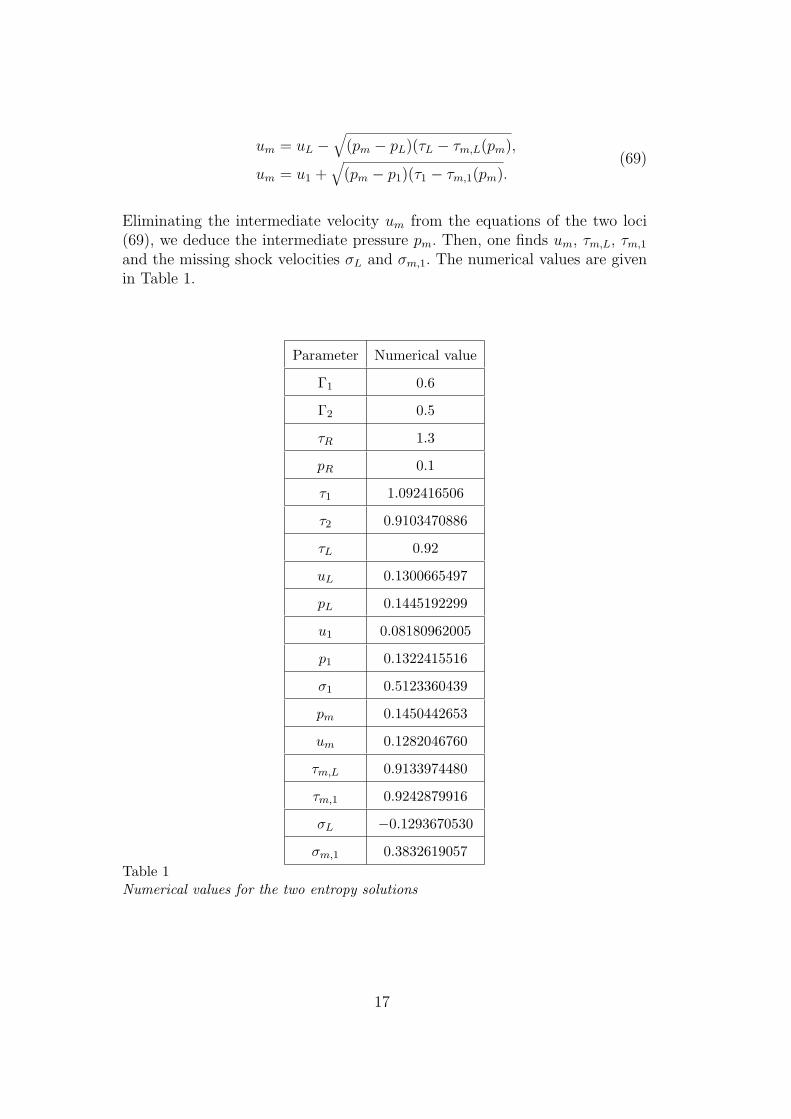
Eliminating the intermediate velocity um from the equations of the two loci(69), we deduce the intermediate pressure pm. Then, one finds um, τm,L, τm,1

and the missing shock velocities σL and σm,1. The numerical values are givenin Table 1.

Parameter Numerical value

Γ1 0.6

Γ2 0.5

τR 1.3

pR 0.1

τ1 1.092416506

τ2 0.9103470886

τL 0.92

uL 0.1300665497

pL 0.1445192299

u1 0.08180962005

p1 0.1322415516

σ1 0.5123360439

pm 0.1450442653

um 0.1282046760

τm,L 0.9133974480

τm,1 0.9242879916

σL −0.1293670530

σm,1 0.3832619057Table 1Numerical values for the two entropy solutions

17

5 A simple finite volume scheme for the simulation of cavitatingflows

In this section, we present numerical results in one dimension obtained with anew projection finite volume scheme. By projection, or relaxation, scheme wemean that each time step is made of two sub-steps. In the first sub-step a clas-sical conservative scheme is employed. Thus, in this stage, the phase transitionis not taken into account. Because the pressure law is simplified, it is possibleto use an exact Riemann solver and to have the correct entropy dissipation. Inthe second sub-step, the projection step, some variables are modified in orderto stick to the equilibrium pressure law. This stage is conservative, becausethe density, velocity and energy are not modified. It is also entropy dissipa-tive by construction. This approach is very similar to the Boltzmann schemeapproach: see [23] and included references.

We shall present three results.

We first consider the test case of a double rarefaction wave in a water flow.If the phase transition is not taken into account, we observe that the densityof water, even in the rarefaction region, remains of the order of 1000kg.m−3

and that the pressure becomes strongly negative. The first result is obtainedwith the stiffened gas mixture model defined by the entropy (46). The phasetransition is not taken into account and we wish to test the appearance ofnegative pressures or tensions in the liquid.

In the second test, we activate phase transition. We test the appearance ofa bubble of vapor in a liquid subject to a strong drop of pressure. The pres-sure law coefficients that we use are based on physical measurements and aredetailed in Table 4.

In the third test, we try to compute the analytical solution constructed inSection 4.2. We thus limit ourselves to a mixture of perfect gases whose entropyis given by (52).

For the conservative scheme in the first sub-step, we use the classical Godunovscheme. It is based on an exact Riemann solver for the problem:

vt + f(v)x = 0, v(0, x) =

vL if x < 0,

vR if x > 0.

For the stiffened gas mixture, the conservative variables are v = (ρ, ρu, ρε +ρu2

2, ρα, ρy)T , the flux is f(v) = (ρu, ρu2 + p, (ρε + ρu2

2+ p)u, ραu, ρyu)T . The

pressure law is given by (40-45).

18

For the perfect gas model, the volume fraction α and the corresponding partof the flux are useless, because we have already supposed the pressure equi-librium.

We denote by R(xt, vL, vR) the self-similar solution v. As studied in [4], the

Riemann problem has a unique global entropic solution.

Let h be a space step and τ a time step. Let xi = ih, tn = nτ and wni '

w(tn, xi) where w is an entropic solution of wt + f(w)x = 0. The classicalGodunov step is

wn+1/2i − wn

i

τ+

F ni+1/2 − F n

i−1/2

h= 0, (70)

withF n

i+1/2 = f(R(0, wn

i , wni+1

). (71)

This first step provides us with a density ρn+1 = ρn+1/2, a velocity un+1 =un+1/2 and an internal energy εn+1 = εn+1/2. The volume fraction αn+1/2 andthe mass fraction yn+1/2 have to be updated (projected) to take into accountphase transition. In order to go back to the equilibrium pressure law, we thusdefine (αn+1, yn+1) by

s(1/ρn+1, εn+1, αn+1, yn+1) = max(α,y)∈[0,1]×[0,1]

s(1/ρn+1, εn+1, α, y). (72)

For the perfect gas model the volume fraction is not present and we optimizeonly with respect to the mass fraction y.

5.1 Numerical results for the metastable case

In order to illustrate our approach, we first recall what happens if cavitationis not taken into account. The test case is a Riemann problem which presentstwo rarefaction waves in water. It is intended to demonstrate the occurenceof negative pressures when cavitation is not taken into account. The physicaljustification is detailed in [11]. The Riemann problem with negative pressuresis solved in [4].

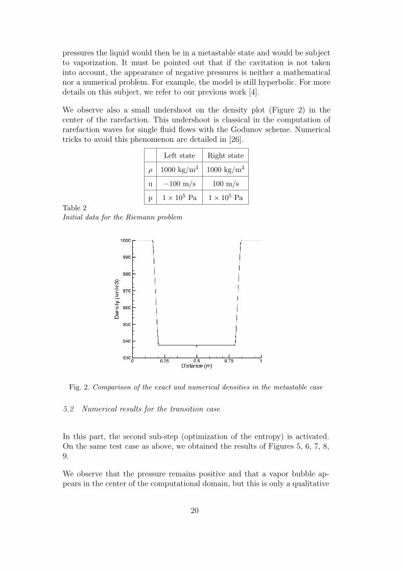
The simulation time is 0.2 ms, the discretization is of 1000 cells. The lengthof the computational domain is 1 m. The initial data are given in Table 2,and the numerical parameters for the stiffened gas law are given in Table 4.The numerical results are on Figures 2, 3, 4. We observe two rarefaction wavesmoving in opposite directions and the appearance of negative pressures inthe rarefied region. Actually, negative pressures can locally and briefly appearin a liquid, they should then be called tensions. But in the zone of negative

19

pressures the liquid would then be in a metastable state and would be subjectto vaporization. It must be pointed out that if the cavitation is not takeninto account, the appearance of negative pressures is neither a mathematicalnor a numerical problem. For example, the model is still hyperbolic. For moredetails on this subject, we refer to our previous work [4].

We observe also a small undershoot on the density plot (Figure 2) in thecenter of the rarefaction. This undershoot is classical in the computation ofrarefaction waves for single fluid flows with the Godunov scheme. Numericaltricks to avoid this phenomenon are detailed in [26].

Left state Right state

ρ 1000 kg/m3 1000 kg/m3

u −100 m/s 100 m/s

p 1× 105 Pa 1× 105 PaTable 2Initial data for the Riemann problem

Fig. 2. Comparison of the exact and numerical densities in the metastable case

5.2 Numerical results for the transition case

In this part, the second sub-step (optimization of the entropy) is activated.On the same test case as above, we obtained the results of Figures 5, 6, 7, 8,9.

We observe that the pressure remains positive and that a vapor bubble ap-pears in the center of the computational domain, but this is only a qualitative

20

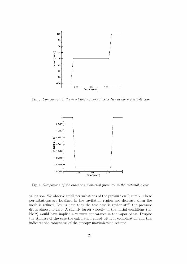
Fig. 3. Comparison of the exact and numerical velocities in the metastable case

Fig. 4. Comparison of the exact and numerical pressures in the metastable case

validation. We observe small perturbations of the pressure on Figure 7. Theseperturbations are localized in the cavitation region and decrease when themesh is refined. Let us note that the test case is rather stiff: the pressuredrops almost to zero. A slightly larger velocity in the initial conditions (ta-ble 2) would have implied a vacuum appearance in the vapor phase. Despitethe stiffness of the case the calculation ended without complication and thisindicates the robustness of the entropy maximization scheme.

21

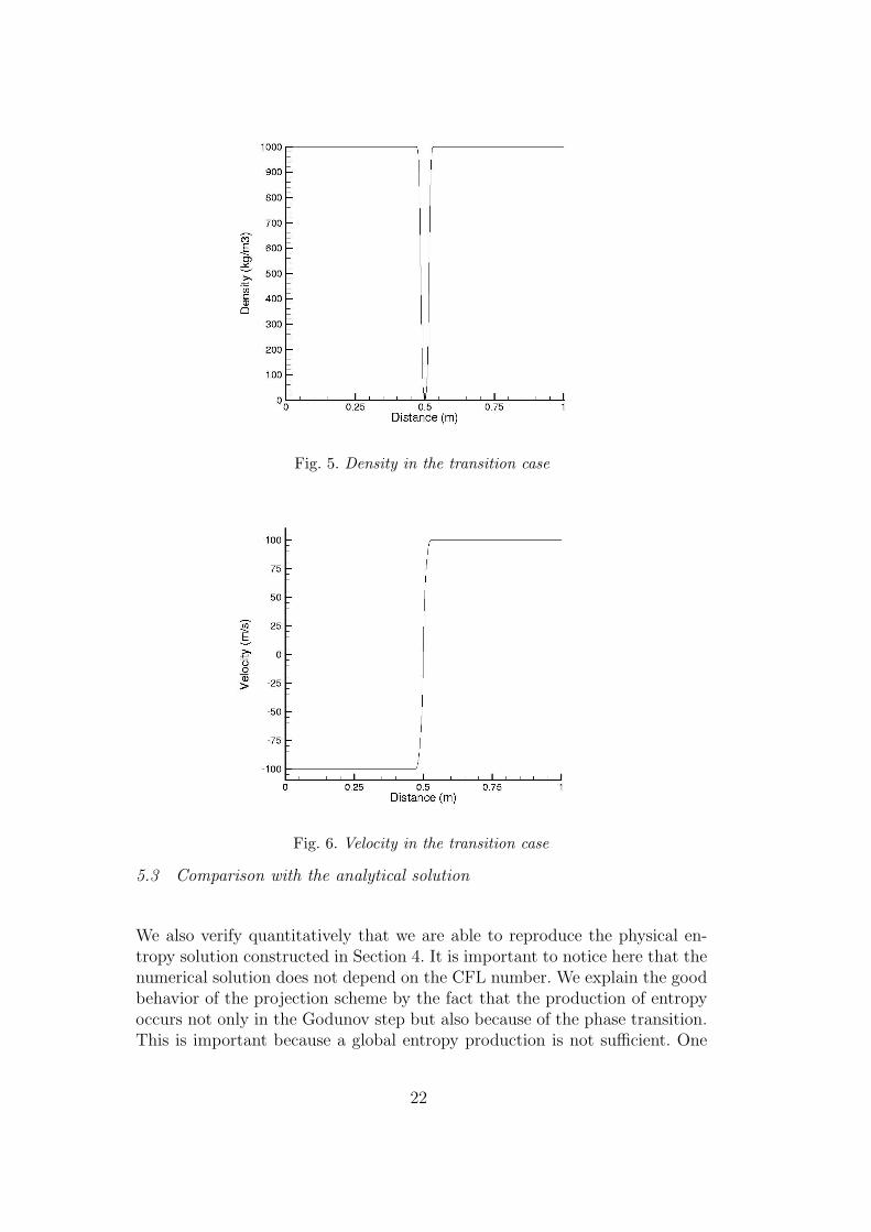
Fig. 5. Density in the transition case

Fig. 6. Velocity in the transition case

5.3 Comparison with the analytical solution

We also verify quantitatively that we are able to reproduce the physical en-tropy solution constructed in Section 4. It is important to notice here that thenumerical solution does not depend on the CFL number. We explain the goodbehavior of the projection scheme by the fact that the production of entropyoccurs not only in the Godunov step but also because of the phase transition.This is important because a global entropy production is not sufficient. One

22

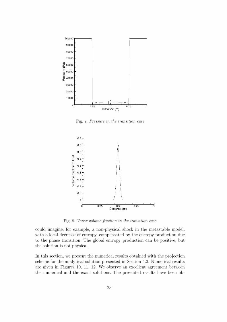
Fig. 7. Pressure in the transition case

Fig. 8. Vapor volume fraction in the transition case

could imagine, for example, a non-physical shock in the metastable model,with a local decrease of entropy, compensated by the entropy production dueto the phase transition. The global entropy production can be positive, butthe solution is not physical.

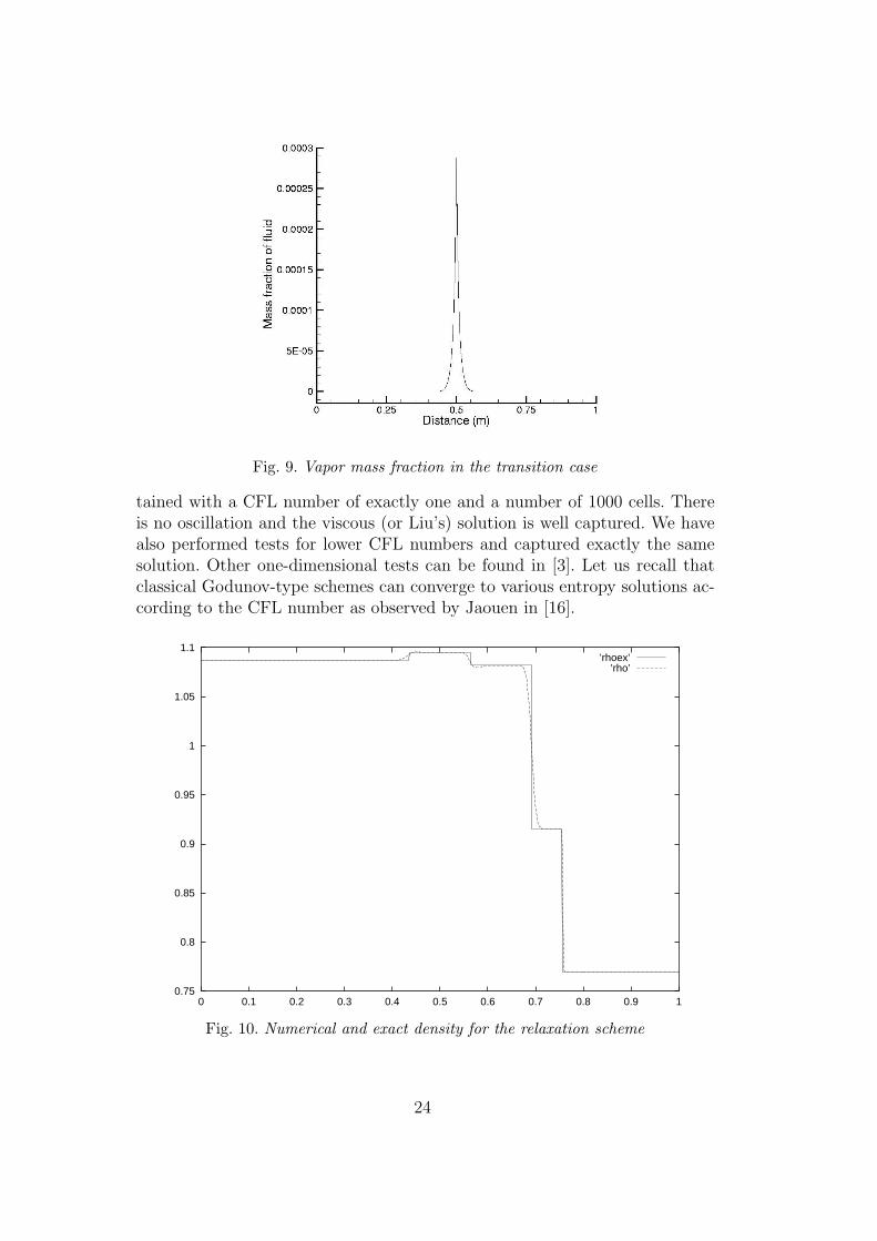
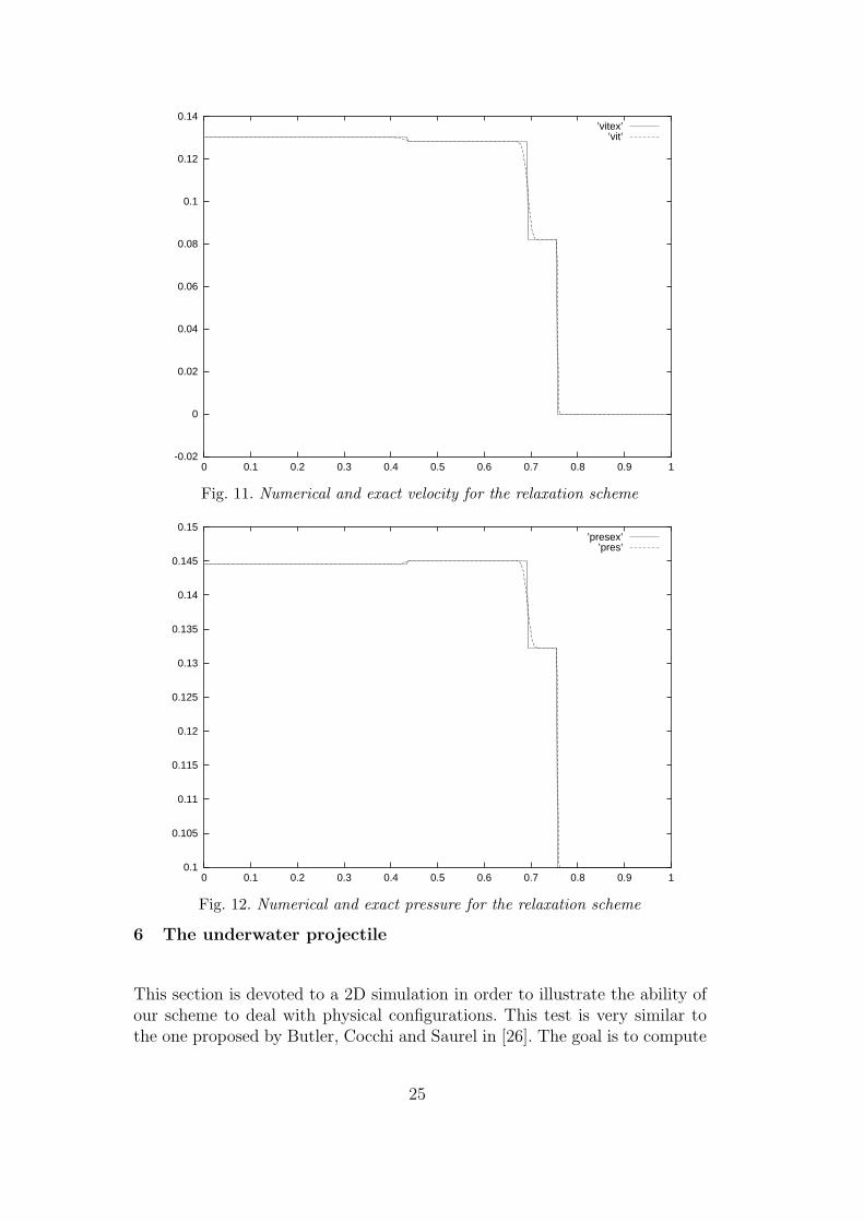
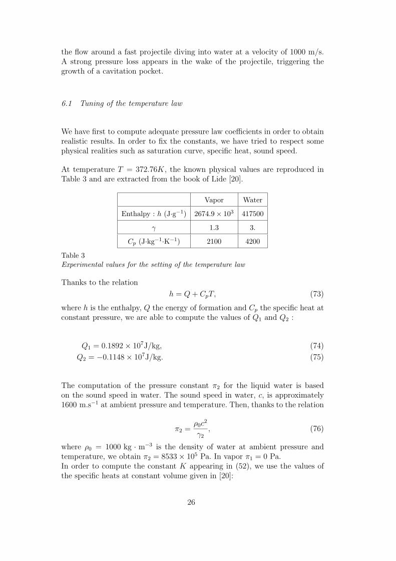
In this section, we present the numerical results obtained with the projectionscheme for the analytical solution presented in Section 4.2. Numerical resultsare given in Figures 10, 11, 12. We observe an excellent agreement betweenthe numerical and the exact solutions. The presented results have been ob-

23

Fig. 9. Vapor mass fraction in the transition case

tained with a CFL number of exactly one and a number of 1000 cells. Thereis no oscillation and the viscous (or Liu’s) solution is well captured. We havealso performed tests for lower CFL numbers and captured exactly the samesolution. Other one-dimensional tests can be found in [3]. Let us recall thatclassical Godunov-type schemes can converge to various entropy solutions ac-cording to the CFL number as observed by Jaouen in [16].

0.75

0.8

0.85

0.9

0.95

1

1.05

1.1

0 0.1 0.2 0.3 0.4 0.5 0.6 0.7 0.8 0.9 1

’rhoex’’rho’

Fig. 10. Numerical and exact density for the relaxation scheme

24

-0.02

0

0.02

0.04

0.06

0.08

0.1

0.12

0.14

0 0.1 0.2 0.3 0.4 0.5 0.6 0.7 0.8 0.9 1

’vitex’’vit’

Fig. 11. Numerical and exact velocity for the relaxation scheme

0.1

0.105

0.11

0.115

0.12

0.125

0.13

0.135

0.14

0.145

0.15

0 0.1 0.2 0.3 0.4 0.5 0.6 0.7 0.8 0.9 1

’presex’’pres’

Fig. 12. Numerical and exact pressure for the relaxation scheme

6 The underwater projectile

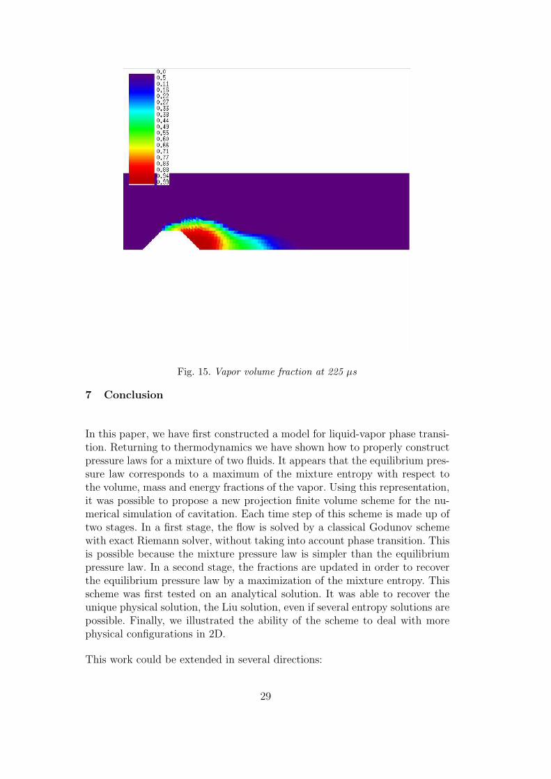
This section is devoted to a 2D simulation in order to illustrate the ability ofour scheme to deal with physical configurations. This test is very similar tothe one proposed by Butler, Cocchi and Saurel in [26]. The goal is to compute

25

the flow around a fast projectile diving into water at a velocity of 1000 m/s.A strong pressure loss appears in the wake of the projectile, triggering thegrowth of a cavitation pocket.

6.1 Tuning of the temperature law

We have first to compute adequate pressure law coefficients in order to obtainrealistic results. In order to fix the constants, we have tried to respect somephysical realities such as saturation curve, specific heat, sound speed.

At temperature T = 372.76K, the known physical values are reproduced inTable 3 and are extracted from the book of Lide [20].

Vapor Water

Enthalpy : h (J·g−1) 2674.9× 103 417500

γ 1.3 3.

Cp (J·kg−1·K−1) 2100 4200

Table 3Experimental values for the setting of the temperature law

Thanks to the relation

h = Q + CpT, (73)

where h is the enthalpy, Q the energy of formation and Cp the specific heat atconstant pressure, we are able to compute the values of Q1 and Q2 :

Q1 = 0.1892× 107J/kg, (74)

Q2 = −0.1148× 107J/kg. (75)

The computation of the pressure constant π2 for the liquid water is basedon the sound speed in water. The sound speed in water, c, is approximately1600 m.s−1 at ambient pressure and temperature. Then, thanks to the relation

π2 =ρ0c

2

γ2

, (76)

where ρ0 = 1000 kg · m−3 is the density of water at ambient pressure andtemperature, we obtain π2 = 8533× 105 Pa. In vapor π1 = 0 Pa.In order to compute the constant K appearing in (52), we use the values ofthe specific heats at constant volume given in [20]:

26

Cv,1 =Cp,1

γ1

= 1615.38 J.kg−1.K−1 (77)

Cv,2 =Cp,2

γ2

= 1400 J.kg−1.K−1 (78)

Finally, the constant K is obtained by

K = (Cv,1 − Cv,2) ln(T0) + (79)

(Q2 −Q1)

T0

+ (γ1 − 1)Cv,1 ln

((γ1 − 1)Cv,1T0

(p0 + π1)

)(80)

−(γ2 − 1)Cv,2 ln

((γ2 − 1)Cv,2T0

(p0 + π2)

),

The ambient pressure is p0 = 105Pa and the ambient temperature T0 =273.76K.

The physical constants of the stiffened gases model are summed up in Table4.

fluid 1 (vapor) fluid 2 (water)

γ 1.3 3

π 0 8533 bar

Q 0.1892×107 J/kg -0.1148×107J/kg

Cv 1615.38 J/kg/K 1400 J/kg/KTable 4Constants in the stiffened gas model

6.2 Numerical results

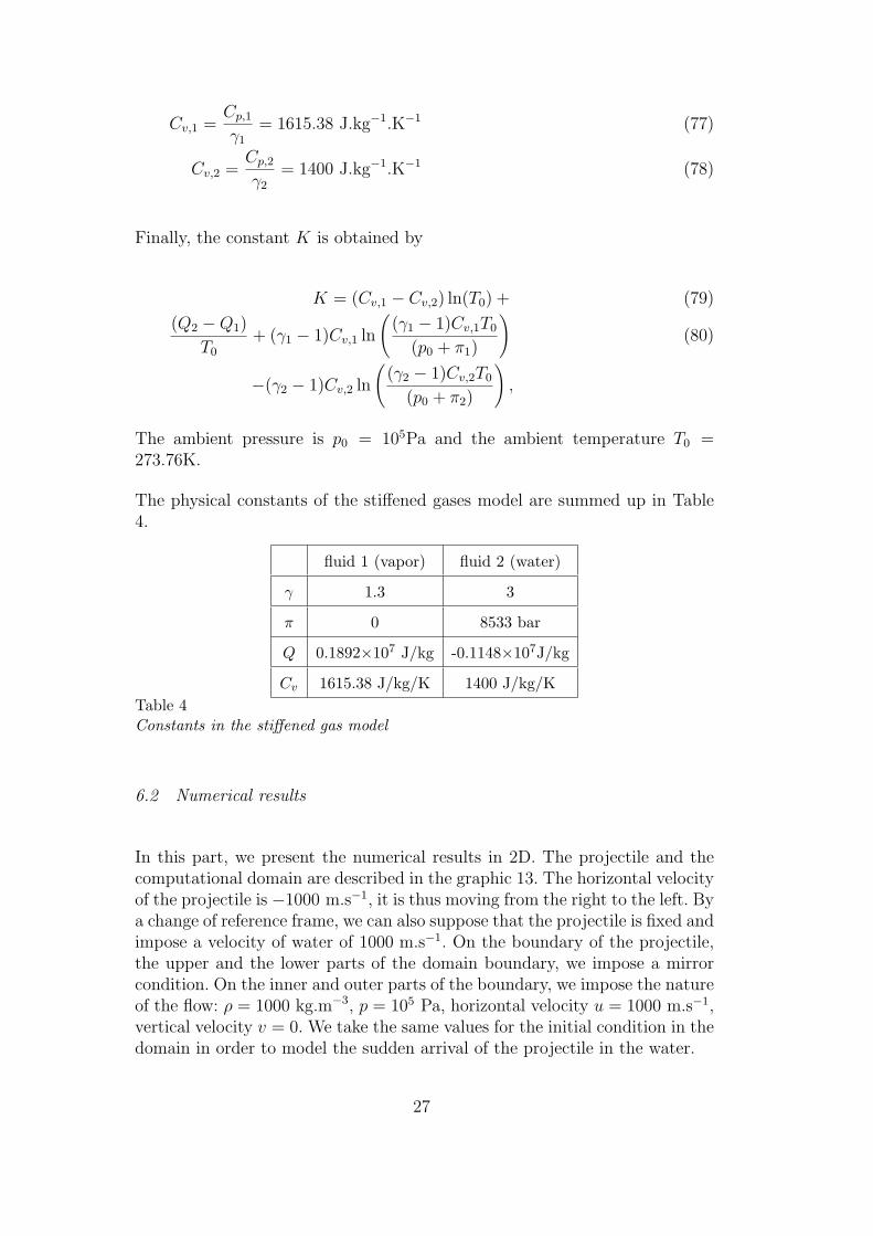
In this part, we present the numerical results in 2D. The projectile and thecomputational domain are described in the graphic 13. The horizontal velocityof the projectile is −1000 m.s−1, it is thus moving from the right to the left. Bya change of reference frame, we can also suppose that the projectile is fixed andimpose a velocity of water of 1000 m.s−1. On the boundary of the projectile,the upper and the lower parts of the domain boundary, we impose a mirrorcondition. On the inner and outer parts of the boundary, we impose the natureof the flow: ρ = 1000 kg.m−3, p = 105 Pa, horizontal velocity u = 1000 m.s−1,vertical velocity v = 0. We take the same values for the initial condition in thedomain in order to model the sudden arrival of the projectile in the water.

27

Fig. 13. Geometry description

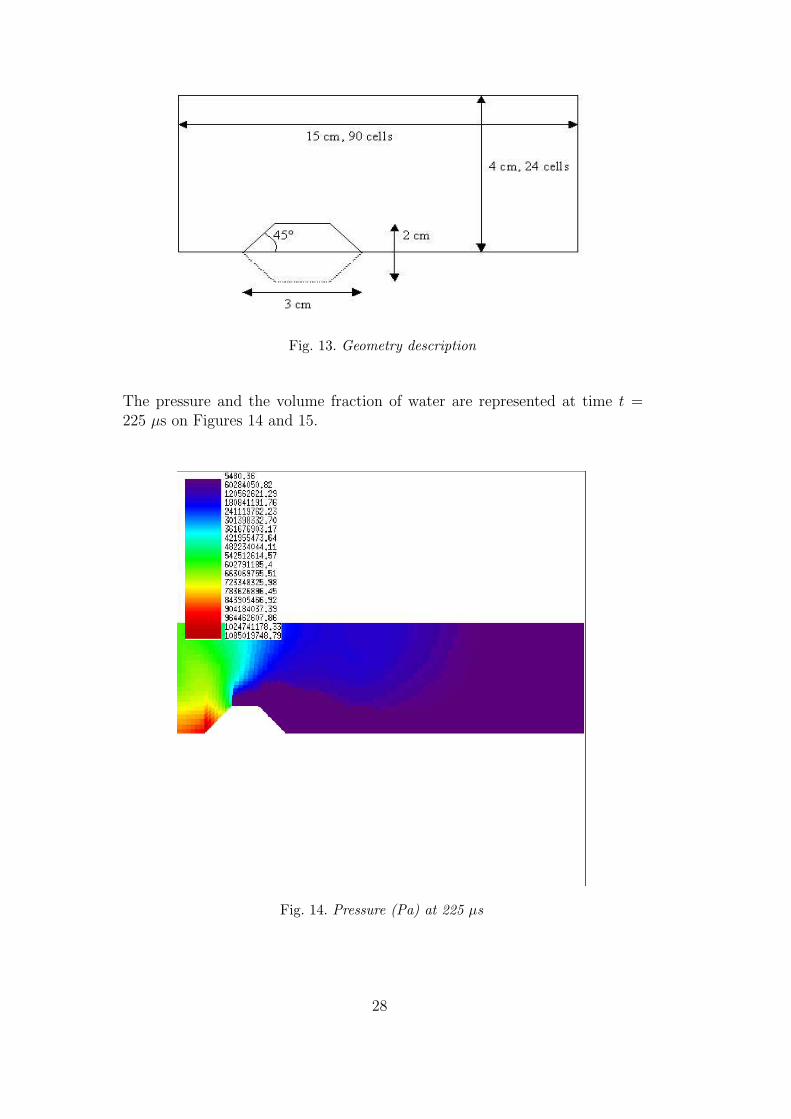
The pressure and the volume fraction of water are represented at time t =225 µs on Figures 14 and 15.

Fig. 14. Pressure (Pa) at 225 µs

28

Fig. 15. Vapor volume fraction at 225 µs

7 Conclusion

In this paper, we have first constructed a model for liquid-vapor phase transi-tion. Returning to thermodynamics we have shown how to properly constructpressure laws for a mixture of two fluids. It appears that the equilibrium pres-sure law corresponds to a maximum of the mixture entropy with respect tothe volume, mass and energy fractions of the vapor. Using this representation,it was possible to propose a new projection finite volume scheme for the nu-merical simulation of cavitation. Each time step of this scheme is made up oftwo stages. In a first stage, the flow is solved by a classical Godunov schemewith exact Riemann solver, without taking into account phase transition. Thisis possible because the mixture pressure law is simpler than the equilibriumpressure law. In a second stage, the fractions are updated in order to recoverthe equilibrium pressure law by a maximization of the mixture entropy. Thisscheme was first tested on an analytical solution. It was able to recover theunique physical solution, the Liu solution, even if several entropy solutions arepossible. Finally, we illustrated the ability of the scheme to deal with morephysical configurations in 2D.

This work could be extended in several directions:

29

(1) First of all, it would be interesting to improve the precision of the mixturelaw. Indeed, in its present form, the model is only valid below the criticalpoint. The critical point is a special point of the phase diagram in thetemperature-pressure plane. It corresponds to the upper extremity of thesaturation curve. Beyond this point there is no more distinction betweenthe two phases. We hope that this behavior can be modelled, at leastroughly, by only changing the entropy function of the liquid phase.

(2) Another interesting extension would be to add a supplementary inertphase in order to simulate, for instance, air-water flows, with the possi-bility to observe a cavitation phenomenon in water. The model is a simpleextension of what is done in Section 2.3. The mixture entropy is the sumof the three phases entropies, as in formula (29), and depends on density,internal energy, air fractions and vapor fractions. In the optimization pro-cess, we maximize the mixture entropy with respect to all the fractionsexcluding the mass fraction of air, because there is no mass transfer be-tween air and water. The mass fraction of air is thus simply convected.Despite its simplicity this approach leads to numerical difficulties. Ac-cording to our first experiments, numerical pressure oscillations appearat the interface between air and water [3]. These oscillations are similar tothose observed in many works about two-phase flows [1], [17], [25], [29]...It must be pointed out that in the present work we observed no pressureoscillations at the interface between liquid and vapor for we have allowedmass transfers between these two phases. The maximization of entropyensures the good stability of the numerical scheme. On the other hand,if the optimization with respect to one variable is omitted (it would bethe case for an interface without mass transfer), it is sufficient to implyoscillations.

(3) Finally, it appears that the equilibrium hypothesis is physically not truefor very fast flows. It is even possible to observe during a short timenegative pressures in the liquid before the phase transition [11]. It is clearthat one should then give a finite value to the parameter λ in the sourceterm (17). This value is linked to the time scale of the phase transition.Instead of solving numerically an ordinary differential equation one couldimagine for instance to perform only a partial optimization of the mixtureentropy.

References

[1] R. Abgrall. Generalisation of the Roe scheme for the computation of mixtureof perfect gases. Recherche Aerospatiale, 6:31–43, 1988.

[2] S. Andreae, J. Ballmann, S. Muller, and A. Voss. Dynamics of collapsing bubblesnear walls. In Ninth International Conference on Hyperbolic Problems. IGPM,RWTH Aachen, 2002.

30

[3] T. Barberon. Modelisation mathematique et numerique de la cavitation dansles ecoulements multiphasiques compressibles. PhD thesis, Universite de Toulon,2002.

[4] T. Barberon, P. Helluy, and S. Rouy. Practical computation of axisymmetricalmultifluid flows. International Journal of Finite Volumes, 1(1):1–34, 2003.

[5] H. Bethe. The theory of shock waves for an arbitrary equation of state. Technicalreport, US department of commerce, 1942.

[6] H. B. Callen. Thermodynamics and an introduction to thermostatistics, secondedition. Wiley and Sons, 1985.

[7] G. Chanteperdrix, P. Villedieu, and Vila J.-P. A compressible model forseparated two-phase flows computations. In ASME Fluids Engineering DivisionSummer Meeting. ASME, Montreal, Canada, July 2002.

[8] J.-P. Cocchi and R. Saurel. A Riemann problem based method for theresolution of compressible multimaterial flows. Journal of ComputationalPhysics, 137(2):265–298, 1997.

[9] F. Coquel and B. Perthame. Relaxation of energy and approximate Riemannsolvers for general pressure laws in fluid dynamics. SIAM J. Numer. Anal.,35(6):2223–2249 (electronic), 1998.

[10] J.-P. Croisille. Contribution a l’etude theorique et a l’approximationpar elements finis du systeme hyperbolique de la dynamique des gazmultidimensionnelle et multiespeces. PhD thesis, Universite Paris VI, 1991.

[11] J.-P. Franc et al. La Cavitation: Mecanismes Physiques et Aspects Industriels.Presses Universitaires de Grenoble, 1995.

[12] T. Gallouet, J.-M. Herard, and N. Seguin. Some recent finite volume schemesto compute Euler equations using real gas EOS. Internat. J. Numer. MethodsFluids, 39(12):1073–1138, 2002.

[13] E. Godlewski and P.-A. Raviart. Numerical approximation of hyperbolic systemsof conservation laws. Springer, 1996.

[14] B. T. Hayes and P. G. Lefloch. Nonclassical shocks and kinetic relations: strictlyhyperbolic systems. SIAM J. Math. Anal., 31(5):941–991 (electronic), 2000.

[15] P. Helluy and T. Barberon. Finite volume simulations of cavitating flows. InFinite Volumes for Complex Applications III (Porquerolles, 2002), pages 455–462. Hermes Penton Ltd, London, 2002.

[16] S. Jaouen. Etude mathematique et numerique de stabilite pour des modeleshydrodynamiques avec transition de phase. PhD thesis, Universite Paris VI,November 2001.

[17] S. Karni. Multicomponent flow calculations by a consistent primitive algorithm.J. Comput. Phys., 112(1):31–43, 1994.

31

[18] B. Koren, M. R. Lewis, E. H. van Brummelen, and B. van Leer. Riemann-problem and level-set approaches for homentropic two-fluid flow computations.J. Comput. Phys., 181(2):654–674, 2002.

[19] P. G. LeFloch and C. Rohde. High-order schemes, entropy inequalities, andnonclassical shocks. SIAM J. Numer. Anal., 37(6):2023–2060, 2000.

[20] D. R. Lide et al. Handbook of chemistry and physics, 82nd edition. CRC Press,2001.

[21] T. P. Liu. The Riemann problem for general systems of conservation laws. J.Diff. Equations., 56:218–234, 1975.

[22] R. Menikoff and B. J. Plohr. The Riemann problem for fluid flow of realmaterials. Rev. Modern Phys., 61(1):75–130, 1989.

[23] B. Perthame. Boltzmann type schemes for gas dynamics and the entropyproperty. SIAM J. Numer. Anal., 27(6):1405–1421, 1990.

[24] R. Saurel and R. Abgrall. A multiphase Godunov method for compressiblemultifluid and multiphase flows. J. Comput. Phys., 150(2):425–467, 1999.

[25] R. Saurel and R. Abgrall. A simple method for compressible multifluid flows.SIAM J. Sci. Comput., 21(3):1115–1145, 1999.

[26] R. Saurel, J.P. Cocchi, and P.B. Butler. A numerical study of cavitation in thewake of a hypervelocity underwater projectile. AIAA Journal of Propulsion andPower, 15(4):513–522, 1999.

[27] D. Serre. Systemes de lois de conservation I et II. Diderot Editeur, 1996.

[28] E. F. Toro. Riemann solvers and numerical methods for fluid dynamics, 2ndedition. Springer, 1999.

[29] E. H. van Brummelen and B. Koren. A pressure-invariant conservativeGodunov-type method for barotropic two-fluid flows. Journal of ComputationalPhysics, 185:289–308, 2003.

[30] B. Wendroff. The Riemann problem for materials with non-convex equationsof state: II, general flows. J. Math. Anal. Appl., 38:640–658, 1972.

[31] H. Weyl. Shock waves in arbitrary fluids. Com. Pure Appl. Math., 103(2):103–122, 1949.

32