Firm Beliefs and Long-run Demand Effects in a Labor-Constrained Model of Growth and Distribution Daniele Tavani * , Luke Petach † May 24, 2019 Abstract One of the most debated questions in alternative macroeconomics regards whether demand policies have permanent or merely transitory effects. While demand matters in the long run in (neo-) Kaleckian economics, both economists operating within other Keynesian traditions (e.g. Skott, 1989) as well as Classical economists (Dum´ enil and L´ evy, 1999) argue that in the long-run output growth is constrained by an exogenous, ‘natural’ rate. This paper attempts to bridge the gap by analyzing the role of firm beliefs about the state of the economy in a labor-constrained growth and distribution model based on Kaldor (1956) and Goodwin (1967). The main innovation is the in- clusion of beliefs about economic activity in an explicitly dynamic choice of capacity utilization at the firm level. We show that: (i) the relevance of such beliefs generates an inefficiently low utilization rate and labor share in equilibrium; but (ii) the efficient utilization rate can be implemented through fiscal policy. Under exogenous techni- cal change, (iii) the inefficiency does not affect the equilibrium employment rate and growth rate, but expansionary fiscal policy has positive level effects on both GDP and the labor share. However, (iv) with endogenous technical change ` a la Verdoorn (1949), fiscal policy has also temporary growth effects. Finally, (v) the fact that the choice of utilization responds to income shares has a stabilizing effect on growth cycles, even under exogenous technical change, that is analogous to factor substitution. —————————————————— JEL Codes: D25, E12, E22, E25, E62. Keywords: Beliefs, Capacity Utilization, Factor Shares, Growth Cycles. * Corresponding Author. Department of Economics, Colorado State University. 1771 Campus Delivery, Fort Collins, CO 80523-1771. Email:[email protected]. † Jack C. Massey College of Business, Belmont University. Email: [email protected]1
Transcript
Firm Beliefs and Long-run Demand Effects in aLabor-Constrained Model of Growth and
Distribution
Daniele Tavanilowast Luke Petachdagger
May 24 2019
Abstract
One of the most debated questions in alternative macroeconomics regards whetherdemand policies have permanent or merely transitory effects While demand mattersin the long run in (neo-) Kaleckian economics both economists operating within otherKeynesian traditions (eg Skott 1989) as well as Classical economists (Dumenil andLevy 1999) argue that in the long-run output growth is constrained by an exogenouslsquonaturalrsquo rate This paper attempts to bridge the gap by analyzing the role of firmbeliefs about the state of the economy in a labor-constrained growth and distributionmodel based on Kaldor (1956) and Goodwin (1967) The main innovation is the in-clusion of beliefs about economic activity in an explicitly dynamic choice of capacityutilization at the firm level We show that (i) the relevance of such beliefs generatesan inefficiently low utilization rate and labor share in equilibrium but (ii) the efficientutilization rate can be implemented through fiscal policy Under exogenous techni-cal change (iii) the inefficiency does not affect the equilibrium employment rate andgrowth rate but expansionary fiscal policy has positive level effects on both GDP andthe labor share However (iv) with endogenous technical change a la Verdoorn (1949)fiscal policy has also temporary growth effects Finally (v) the fact that the choice ofutilization responds to income shares has a stabilizing effect on growth cycles evenunder exogenous technical change that is analogous to factor substitution
lowastCorresponding Author Department of Economics Colorado State University 1771 Campus DeliveryFort Collins CO 80523-1771 EmailDanieleTavaniColostateedudaggerJack C Massey College of Business Belmont University Email LukePetachBelmontedu
1
1 Introduction
One of the most debated questions in alternative macroeconomics regards whether demandpolicies have permanent or merely transitory effects While Kaleckian economists haveargued that demand matters even in the long run both economists operating within otherKeynesian traditionsmdashsuch as Harrodians (eg Skott 1989 2010 2012 2017)mdashas wellas Classical economists (Dumenil and Levy 1999) argue that long-run output growth isconstrained by the so-called natural rate Moreover it is argued the long-run rate of uti-lization of installed capacity which proxies for effective demand in these frameworks mustnecessarily be exogenous With fully adjusted exogenous utilization and growth fixed atthe natural rate many of the central results of canonical Kaleckian models appear to be injeopardy the paradox of thrift the paradox of costs and the relevance of effective demandin the long-run may no longer hold The latter is especially concerning given its centralityfor (post-) Keynesian economics
This is not just an academic dispute considerations about lackluster aggregate demandhave been especially relevant in the aftermath of the Great Recession and the sluggishrecovery that followed in most of the worldrsquos advanced economies Figure 1 plots realGDP in the United States against the Congressional Budget Office estimates of potentialoutput in 2007 and the revised CBO estimates in 2017 The downward revision of potentialoutput points to the presence of considerable slack capacity in the US economy over adecade after the Great Recession ended (Fatas 2019)
Figure 1 US Real GDP (billions of chained US dollars black) vs the CBO estimates ofpotential GDP in 2007 (gray) and the CBO estimates of potential GDP in 2017 (dashed)Source Congressional Budget Office
2000 2005 2010 2015
12000
13000
14000
15000
16000
17000
18000
RealGDP
Such observations point to the question if one takes the objections of the Harrodian
2
and Classical perspectives seriously is it necessary to abandon hope for the possibility ofa meaningful role for effective demand in the medium-to-long run Our answer is noWhile the Classical demarcation limiting the effectiveness of demand policy to the short-runmdashwhich has led Dumenil and Levy (1999) to a description of the world as ldquoshort-runKeynesian long-run Classicalrdquomdashmay be analytically useful it is unlikely to hold true inactually existing capitalist economies Michl (2017) then points out that a key task foralternative economic theories is to engage in what theologians call ldquoirenicsrdquo or the processof reconciling conflicting doctrines in order to paint a more realistic picture of the spacecapitalist economies actually inhabitmdasha space which undoubtedly combines elements ofboth the Classical and Keynesian visions (p74)
Our task in this paper is thus to develop a micro-to-macro fully Classical model fea-turing an explicit dynamic choice of utilization at the firm level in order to illustrate amechanism that may give rise to lackluster economic performance as an equilibrium out-come Our argument is that if firms formulate beliefs about the state of the economy whenselecting their own level of capacity utilization then demand policies can certainly affectthe level of economic activity in the long-runmdashdespite growth being fixed at the naturalrate The inclusion of beliefs in our model harkens back to the central role that expecta-tions play in the process of employment determination envisioned by Keynes (1936) in The
General Theory ldquo[T]odayrsquos employment can be correctly described as being governed bytodayrsquos expectations taken in conjunction with todayrsquos capital equipmentrdquo (p50) Despitethe central role afforded to the process of expectations-formation by Keynes (1936) rela-tively little effort has been put forth in formalizing beliefs in (post-) Keynesian models withan explicit microeconomic structure Borrowing insights from the literature on coordina-tion games (Cooper 1999) we will show that firm-level beliefs about economic activitycan be captured in a simple way by including (expectations about) the aggregate utilizationrate in the economy as a signal for the current level of effective demand To gain intuitionconsider the following scenario Suppose an individual firm operating at its desired utiliza-tion expects other firms to increase production because the economy is picking up steamIf such beliefs about other firmsrsquo behavior did not have an effect on the firmrsquos own choicethen it must be true that the firm has already maximized its profits and has no incentiveto deviate from the corresponding desired rate of utilization But this cannot be the casebecause the firm can in fact increase its profits by simply utilizing more its capacity in lightof its beliefs about the economy Thus it must be that beliefs enter the choice of utilizationat the firm level
Following Petach and Tavani (2019) we operationalize this assumption extending theKeynesian notion of the user cost of capitalmdashthe opportunity cost incurred by firms when-
3
ever they choose to undertake productionmdashto a more general adjustment cost of operatingequipment First the concept of user cost as outlined by Keynes (1936) is forward-lookingldquo[I]t is the expected sacrifice of future benefit involved in present use which determines theamount of user cost and it is the marginal amount of this sacrifice which determines his(sic) scale of productionrdquo (p70) In other words the user-cost of capital does not merelydepend on the firmrsquos current own-rate of utilization but intertemporal considerations areat play when the choice of utilization is made Thus our rendition of the user cost has anindividual component and it is increasing and convex in the firmrsquos own utilization rate andis embedded in a forward-looking optimization problem Greenwood et al (1988) havealready argued that this individual component captures in a simple but faithful way thefirm-level trade-offs pointed out by Keynes
Second we argue that the cost of utilizing equipment also entails an outward-looking
component which depends on the individual firmrsquos beliefs about the behavior of the aggre-gate economy and motivates our extension of the user cost into a more general adjustmentcost function Thus we introduce a dependence of the cost of utilization on the aggregateutilization rate in the firmrsquos sectormdashor in the economy in the representative firm casemdashinorder to capture the individual firmrsquos incentives to adjust its production given changes inexpectations Specifically we propose a specification of the adjustment cost function wherethe marginal adjustment cost is declining in the average rate of utilization in the economyUnder empirically-sound restrictions (see the results in Petach and Tavani 2019) this for-malization delivers strategic complementarities among firms the desired rate of utilizationat the firm level increases in aggregate utilization it is endogenous to demand in otherwords This feature will produce an equilibrium utilization rate and therefore an equi-librium level of economic activity that is inefficiently low firms will keep some sparecapacity in order to react to the possibility of increased aggregate demand in the economywhile at the same time engaging in the accumulation process
The result can then be used in order to draw policy implications With exogenoustechnical changemdashthe most common specification of technological progress in Harrodianmodelsmdashthe economyrsquos growth rate is exogenously fixed at the natural rate n Accord-ingly there are no growth effects of demand policies However underutilization impliesthat spending policies have positive level effects both on output per worker and the share oflabor The latter will increase in response to spending policies that boost economic activityThus the conclusions of this analysis are that demand matters even in the long run bothfor the level of economic activity and the labor share
In addition to analyzing the effects of demand policies on an economyrsquos balanced growthpath we also consider the implications of incorporating adjustment costs and a strategic
4
choice of capacity utilization for the Goodwin (1967) model whose steady state is virtu-ally identical to Kaldor (1956) but whose focus is on the endless distributive cycle betweenthe employment rate and the labor share The literature has identified four main channelsthrough which the perpetual cycle can be resolved in the long run (i) capitallabor substi-tution along a neoclassical production function (van der Ploeg 1985) (ii) an endogenouslabor-augmenting bias of technical change (Shah and Desai 1981 Foley 2003 Julius2005) (iii) endogenous labor-augmenting innovation financed out of profits (Tavani andZamparelli 2015) and (iv) differential tax rates on capital versus labor incomes in modelswith public infrastructure (Tavani and Zamparelli 2018) In all of these cases the sym-metry in the bargaining positions between capital and labor which is responsible for theendless Goodwin growth cycle (Shah and Desai 1981) is broken in favor of the formerWe show in this paper that the choice of utilization implied by our model acts in the sameway namely turning the resulting steady state from the Goodwin center to a stable focusEssentially the possibility of varying the rate of utilization is analogous to changing thetechnique of production in response to factor shares which is at the heart of the stabilizingchannels discussed in the literature
Finally we also analyze an extension of the model featuring endogenous technicalchange in the form of a Verdoorn law (Verdoorn 1949) the growth rate of labor pro-ductivity depends on the accumulation rate However as it is well-known in the literaturea Verdoorn law delivers a semi-endogenous long-run growth rate it is derived within themodel but is constrained by exogenous parameters such as the growth rate of the labor forceand the Verdoorn pass-through (see the discussion in Tavani and Zamparelli 2017) Differ-ently from the exogenous technical change model however expansionary fiscal policy thatfosters utilization will have a temporary growth effect in addition to its permanent leveleffect Therefore this version of the model shows that demand policies translate mean-ingfully into changes in the growth rate via their impact on the accumulation rate alongthe transition to balanced growth Thus the paper offers one explanation for why tempo-rary demand shocks have permanent level effects under exogenous growth or temporarygrowth effects under endogenous labor-augmenting technical change and offers an addi-tional contribution to the analysis of hysteresis in Classical and Keynesian growth modelsby Setterfield (2018) Michl and Oliver (2019)
2 Basic Elements of the Model
Consider a competitive capitalist firm in a closed economy and assume away the gov-ernment for now Let the firmrsquos production possibilities be summarized by the Leontief
5
technology Y = minuKAL where Y is the firmrsquos output homogeneous with capitalstock K so that we can normalize its price to one u denotes the rate of capacity utiliza-tion L stands for labor A is the current stock of labor-augmenting technologies assumedto grow at the constant rate gA gt 0 in the benchmark model so that the analysis is asclose as possible to baseline Harrodian models such as Skott (1989) and the long-run out-putcapital ratio B is normalized to one for simplicity Time is continuous Maximizingprofits requires to set uK = AL which solves for labor demand L = uKA If the firmpays the same real wage w to each worker the share of wages in output will be equal tothe unit labor cost ω equiv wA Further let the labor force N ge L grow at the constant raten gt 0 Thus the employment rate in the economy e will be equal to LN = uK(AN)
Our main hypothesis is that operating capital equipment entails an adjustment cost λwhich would not be incurred if machinery remained idle (Keynes 1936) First and tocapture the user cost we assume that the adjustment cost increases more than propor-tionally with the firmrsquos own utilization rate u denoting partial derivatives by subscriptsλu gt 0 λuu gt 0 Greenwood et al (1988) have noted that this specification formalizesthe Keynesian effects played by the lsquomarginal efficiency of investmentrsquo and the Keynesiannotion of user cost for the individual firm Second we capture the strategic nature of thechoice of utilization by postulating that the adjustment cost also responds to the firmrsquos be-liefs about the utilization chosen by other firms as captured by u the average utilizationrate We assume that u has a negative impact on the marginal adjustment cost λuu lt 0This assumption implies that the marginal benefit of increasing own utilization increases inthe firmrsquos beliefs about aggregate utilization and is required to generate a strategic com-plementarity which is central in our contribution Petach and Tavani (2019) have offeredstrong and robust empirical support for this assumption using a panel of state-by-sectordata for the United States To sharpen our conclusions we specify a log-linear user costfunction as in Petach and Tavani (2019)
λ(u u) = βu1β uminus
γβ β isin (0 1) γ isin [0 1minus β) (1)
The size of the parameter γ determines the extent to which beliefs about other firmsrsquo be-havior are relevant for the firm choice The special case γ = 0 corresponds to the isolatedfirms case where the choices made by other firms are irrelevant while γ 6= 0 implies astrategic environment in which beliefs matter Further under 0 lt γ lt 1minus β the choice ofutilization generates a (weak) strategic complementarity which will result in a unique non-trivial long-run equilibrium utilization in the model The estimates in Petach and Tavani(2019) strongly support the above parametric restriction that 0 lt γ lt 1minus β
6
In line with the basic Classical and Post Keynesian literature we assume that only profit-earning (capitalist) households save in order to accumulate capital stock However whilein most of the literature capitalists save a constant fraction of their profit incomes at alltimes we follow Foley Michl and Tavani (2019) in assuming that capitalist householdsare forward-looking in their consumption accumulation and utilization decisions Thisassumption is made here in order to rule out any potential lsquoinefficiencyrsquo result implied by alimited planning horizon or by lsquorule of thumbrsquo behavior such as saving the same fractionof income at all times1 Here the capitalist household discounts the future at a constantrate ρ gt 0 derives instantaneous logarithmic utility from its per-period consumption flowdenoted by c(t) and has perfect foresight on the entire planning horizon t isin [sinfin) Finallyassume that there is no independent investment demand function so that capitalist savingsare immediately invested at all times The accumulation constraint omitting the time-dependence for notational simplicity is
K = (1minus ω)uK minus cminus λ(u u)K (2)
Note that increasing the own rate of utilization raises the capitalistrsquos revenues (1minus ω)uKbut also increases the adjustment cost λ(u u) given average utilization As shown in Ap-pendix A the solution to a simple control problem delivers the firm-level choice of ca-pacity utilization as a decreasing function of the labor share while increasing in averageutilization as per equation (3) below The firm-level choice of utilization is equivalent to abest-response function in the game-theoretic sense or a reaction function in Cournot-stylemodels
u(ω u) = (1minus ω)β
1minusβ uγ
1minusβ (3)
Figure 2 displays the behavior of the best-response function in relation to the aggregateutilization rate The intuition for the inverse dependence on the labor share is that anincrease in the latter reduces revenues everything else equal the firm can then cut back onits utilization in order to reduce the user cost of capital On the other hand an increasein aggregate utilization reduces the own marginal adjustment cost everything else equalthus rising the marginal profits that can be made by utilizing more a firmrsquos own installedcapacity the firm can increase utilization up to the point where the marginal benefit ofdoing somdashgiven by (1 minus ω)Kmdashis equal to the marginal user cost λu(u u)K for a givenaverage utilization rate Finally given that the firmrsquos beliefs about aggregate utilizationrepresent expectations about the overall economic activity in the economy the dependence
1Similar reasoning applies to the assumption of competitive firms the results of the model do not dependon slow price adjustments as Skott (2017) has argued to be the case in neo-Kaleckian growth models
7
on average utilization can be thought of as capturing the endogeneity of the firmrsquos desiredrate of utilization to demand Appendix A also shows that the growth rate of consumptionfor the typical capitalist householdmdashwhich describes the household-level saving rulemdashsatisfies
gc equivc
c= (1minus ω)
11minusβ u
γ1minusβ minus ρ (4)
Figure 2 Equilibrium vs efficient utilization rates
U
u = u
U u
u
3 Equilibrium Utilization and Accumulation
An equilibrium growth path is a sequence of quantities c(t) u(t) u(t) k(t)tisin[sinfin) thatsolve the capitalistrsquos control problem given the path for the labor share ω(t)tisin[sinfin) andsuch that u(t) = u(t) for all t The latter requirement requires firms to best-respond to otherfirmsrsquo choices similarly to the notion of a Nash equilibrium Omitting the time notationfor simplicity the equilibrium rate of utilization is easily found as
u(ω) = (1minus ω)β
1minusβminusγ (5)
and is inversely related to the labor share since 1minusβminusγ gt 0 by assumption The intuitionis simple a higher wage share lowers the firmrsquos profits and thus the resources available foraccumulation But the firm can offset the higher wage costs by utilizing less its plants thusreducing the user cost
We can then obtain the equilibrium growth rate by using the condition u = u andimposing balanced growth so that consumption and capital stock grow at the same rate
8
gc = gK = g We haveg = (1minus β)(1minus ω)
1minusγ1minusβminusγ minus ρ (6)
where the first term in the right-hand-side of (6) is the profit rate net of the adjustmentcost Further because of the equilibrium condition u = u the equilibrium adjustment costλ(uu) reduces to the pure user cost of capital ie depreciation
4 The Dynamical System
First consider the economyrsquos share of labor ω = wA Its growth rate will be givenby the difference between the growth rate of the real wage and the growth rate of laborproductivity Following Goodwin (1967) assume that real wages obey a version of thePhillips curve ww = f(e) such that fe gt 0 fee gt 0 In particular we impose f(e) =
ηe1δ η gt 0 δ isin (0 1) Hence the labor share evolves according to
ω
ω= f(e)minus gA (7)
Next consider the employment rate e = uK(AN) Logarithmic differentiation gives
e
e= gK + gu minus (gA + n)
Differentiating (5) we obtain the growth rate of utilization as
u
uequiv gu = minus β
1minus β minus γ
(ω
1minus ω
)ω
ω(8)
so that using the real-wage Phillips curve (7) and the accumulation rate from (6) we find
e =
(1minus β)(1minus ω)
1minusγ1minusβminusγ minus β
1minus β minus γ
(ω
1minus ω
)[f(e)minus gA]minus (ρ+ gA + n)
e (9)
41 Steady State
A steady state is a pair (ωss ess) so that ω = e = 0 Notice that the steady state value ofutilization is uniquely pinned down by the steady state labor share given the equilibriumcondition u = u that delivers equation (5) above The steady state value of the employmentrate is readily found by setting ω = 0 in (7)
ess =
(gAη
)δ(E)
9
The steady state employment rate is fully exogenous because of the exogenous nature oftechnological change in the model On the other hand the steady state value for the laborshare can be solved for in closed form once noting that f(ess) = gA in setting the right-handside of equation (9) equal to zero By so doing we find
1minus ωss =
(ρ+ n+ gA
1minus β
) 1minusβminusγ1minusγ
(Ω)
We can now state a first result of this analysis namely the dependence of steady stateutilization on the capitalist saving rate as a proposition
Proposition 1 The steady state desired utilization rate uss increases in the discount rate ρ
Since the latter reduces savings in the economy the paradox of thrift holds in this model
To prove this result use (5) to solve for the steady state utilization rate as
uss =
(ρ+ n+ gA
1minus β
) β1minusγ
(10)
and partusspartρ gt 0 The result is remarkable because even without an explicit investmentfunction this model delivers a version of the Keynesian paradox of thrift A higher valueof the discount rate ρ reduces the long-run capitalistsrsquo saving the corresponding increasein long-run aggregate consumption can be met by increasing utilization and therefore thesteady-state level of economic activity
42 Stability Analysis
Appendix C shows that unlike the original Goodwin (1967) long-run the steady state ofthis model is locally stable Thus the explicit choice of capacity utilization is an additionalway of breaking the symmetric bargaining positions between capital and labor resolvingthe distributive conflict in the long run (Shah and Desai 1981 van der Ploeg 1985) Figure3 shows the ω = 0 nullcline which is vertical corresponding to the steady state employmentrate ess and is the same at both the equilibrium and the efficient solution and plots the e = 0
nullcline in red The latter is downward sloping and so will be the nullcline correspondingto the efficient growth path as differentiation of the expression in braces in (9) and (13) willshow Notice also that convergence to the steady state is not monotonic the employmentrate which is the forward-looking variable in this model overshoots before convergingto its long-run value In this respect explicit demand shocks (see below) will determinesome short-run cyclical behavior of the system before a new steady state is achieved A
10
time-series plot is displayed in Figure 4
Figure 3 Phase Diagram equilibrium nullclines (red) and efficient e = 0 nullcline (blue)and dynamic trajectories converging to the equilibrium (dotted gray) as opposed to theefficient (solid black) steady state The vector field plot refers to the equilibrium path
ω
ω
ω
ω
5 Welfare and Policy
An interesting feature of this economy is that so long as a (weak) strategic complementar-ity is presentmdashthat is so long as 0 lt γ lt 1 minus βmdashit will generally operate with excesscapacity in equilibrium while at the same time accumulating capital stock To see this letus introduce a benevolent planner solving the accumulation problem under the additionalconstraint that u = u at all times Appendix B proves the following result
Proposition 2 Let γ isin (0 1minus β) Then the efficient choice of utilization is
ulowast(ω) =
(1minus ω1minus γ
) β1minusβminusγ
(11)
and is strictly greater than its decentralized counterpart (5)
Notice that the parameter γ generates a multiplier effect the larger the extent to which firmbeliefs matter the higher the socially-coordinated utilization rate relative to the equilibriumrate Absent a role for beliefs γ = 0 the equilibrium rate and the socially-coordinated rate
11
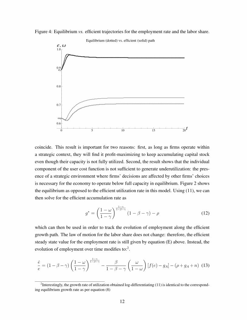
Figure 4 Equilibrium vs efficient trajectories for the employment rate and the labor share
ω
ω
() ()
coincide This result is important for two reasons first as long as firms operate withina strategic context they will find it profit-maximizing to keep accumulating capital stockeven though their capacity is not fully utilized Second the result shows that the individualcomponent of the user cost function is not sufficient to generate underutilization the pres-ence of a strategic environment where firmsrsquo decisions are affected by other firmsrsquo choicesis necessary for the economy to operate below full capacity in equilibrium Figure 2 showsthe equilibrium as opposed to the efficient utilization rate in this model Using (11) we canthen solve for the efficient accumulation rate as
glowast =
(1minus ω1minus γ
) 1minusγ1minusβminusγ
(1minus β minus γ)minus ρ (12)
which can then be used in order to track the evolution of employment along the efficientgrowth path The law of motion for the labor share does not change therefore the efficientsteady state value for the employment rate is still given by equation (E) above Instead theevolution of employment over time modifies to2
e
e= (1minusβminus γ)
(1minus ω1minus γ
) 1minusγ1minusβminusγ
minus β
1minus β minus γ
(ω
1minus ω
)[f(e)minus gA]minus (ρ+ gA +n) (13)
2Interestingly the growth rate of utilization obtained log-differentiating (11) is identical to the correspond-ing equilibrium growth rate as per equation (8)
12
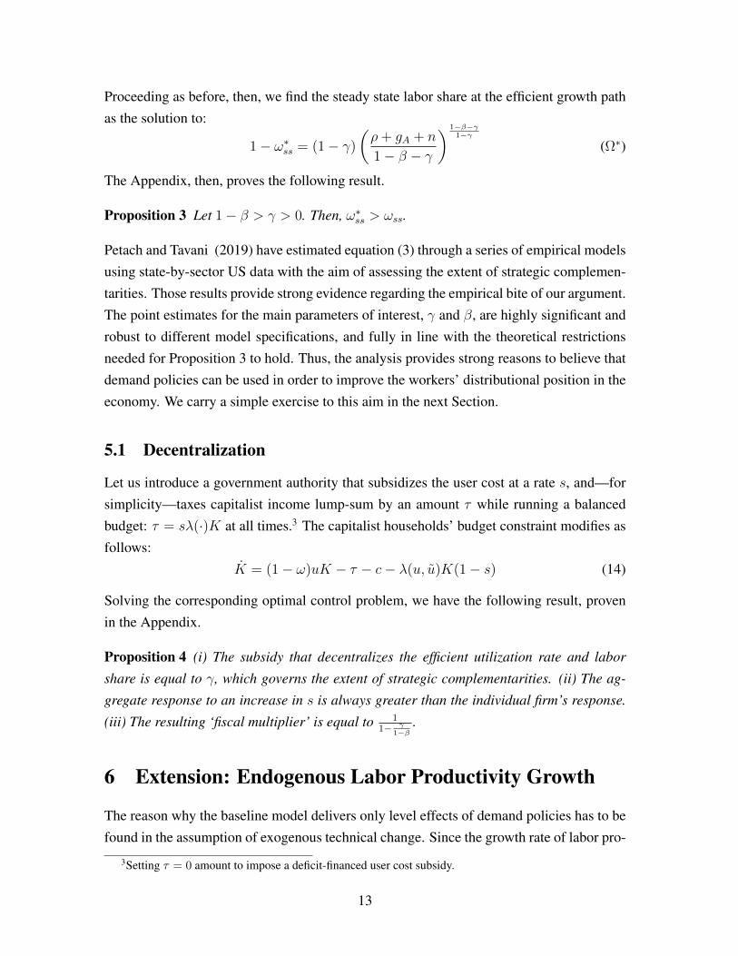
Proceeding as before then we find the steady state labor share at the efficient growth pathas the solution to
1minus ωlowastss = (1minus γ)
(ρ+ gA + n
1minus β minus γ
) 1minusβminusγ1minusγ
(Ωlowast)
The Appendix then proves the following result
Proposition 3 Let 1minus β gt γ gt 0 Then ωlowastss gt ωss
Petach and Tavani (2019) have estimated equation (3) through a series of empirical modelsusing state-by-sector US data with the aim of assessing the extent of strategic complemen-tarities Those results provide strong evidence regarding the empirical bite of our argumentThe point estimates for the main parameters of interest γ and β are highly significant androbust to different model specifications and fully in line with the theoretical restrictionsneeded for Proposition 3 to hold Thus the analysis provides strong reasons to believe thatdemand policies can be used in order to improve the workersrsquo distributional position in theeconomy We carry a simple exercise to this aim in the next Section
51 Decentralization
Let us introduce a government authority that subsidizes the user cost at a rate s andmdashforsimplicitymdashtaxes capitalist income lump-sum by an amount τ while running a balancedbudget τ = sλ(middot)K at all times3 The capitalist householdsrsquo budget constraint modifies asfollows
K = (1minus ω)uK minus τ minus cminus λ(u u)K(1minus s) (14)
Solving the corresponding optimal control problem we have the following result provenin the Appendix
Proposition 4 (i) The subsidy that decentralizes the efficient utilization rate and labor
share is equal to γ which governs the extent of strategic complementarities (ii) The ag-
gregate response to an increase in s is always greater than the individual firmrsquos response
(iii) The resulting lsquofiscal multiplierrsquo is equal to 11minus γ
1minusβ
6 Extension Endogenous Labor Productivity Growth
The reason why the baseline model delivers only level effects of demand policies has to befound in the assumption of exogenous technical change Since the growth rate of labor pro-
3Setting τ = 0 amount to impose a deficit-financed user cost subsidy
13
ductivity is fixed at its exogenous rate gA there are necessarily no growth effects of spend-ing policies aimed at implementing the efficient rate of utilization However economistsworking within alternative traditions (Cornwall and Setterfield 2002 Naastepad 2006Rada 2007 Taylor et al 2018) have long emphasized the possibility of demand shocksaffecting labor productivity growth here we show that a simple extension of the modeldelivers transitory effects of demand shocks on the growth rate of labor productivity in ad-dition to its permanent level effects In line with the contributions mentioned above assumethat labor productivity growth follows a version of Verdoornrsquos law (Verdoorn 1949)4
gA = φgK φ isin (0 1) (15)
While labor productivity growth is endogenous its long run value is anchored by the bal-anced growth condition gA + n = gK so that in the long run we end up with a semi-
endogenous growth rate the growth rate is determined within the model but independentof policy (Jones 1995 1999) In fact we have
gK =n
1minus φ gA =
φn
1minus φ (16)
Importantly however Verdoornrsquos law creates transitory effects of demand policy on laborproductivity growth Both the efficient and the equilibrium accumulation paths converge tothe same growth rate in (16) but the efficient path involves a growth rate of labor productiv-ity that converges from above relative to the equilibrium path as shown in Figure 55 Thisresult points to the additional welfare effects of demand policiesmdashgiven by the integral ofthe distance between the two curvesmdashalong the transition to balanced growth Thus evenif it only impacts the level of output in the long-run demand policy may nonetheless havepermanent positive effects on social welfare via its impact on productivity growth duringthe transition to the steady-state
For completeness let us evaluate the steady state of the extended model Incorporatingequation (15) into the dynamical system (7)-(9) and solving for the steady state income
4In the conventional AK-growth literature the stock of labor-augmenting technologies depends on theaggregate capital stock A = ζKφ ζ gt 0 φ isin (0 1) through a learning-by-doing externality Log-differentiation of this expression gives equation (15) See Romer (1987)
5The figure uses the same parameter calibration as the baseline model plus a value of φ that ensures along-run growth rate of 3 It is displayed for illustrative purposes and it is not meant to argue that demandpolicies can boost labor productivity growth up to over 12 as a literal interpretation of the figure wouldsuggest
14
Figure 5 Equilibrium (gray) vs efficient (black) path of labor productivity growth givenan initial condition on the labor share with a Verdoorn effect
shares and employment rate corresponding to an equilibrium path gives
1minus ωss =
[n+ ρ(1minus φ)
(1minus β)(1minus φ)
] 1minusβminusγ1minusγ
(17)
ess =
[φn
η(1minus φ)
]δ(18)
The efficient path solves for the same long-run employment rate as (18) but delivers thefollowing long-run distribution of income
1minus ωlowastss = (1minus γ)
[n+ ρ(1minus φ)
(1minus β minus γ)(1minus φ)
] 1minusβminusγ1minusγ
(19)
and Proposition 3 holds in this version of the model too6
7 Conclusion
In this paper we have offered one potential resolution to what Michl (2017) calls the ldquodis-cord in the marriage of Classical and Keynesian economics that defines modern heterodoxmacroeconomicsrdquo (p77) Namely the discord caused by conflicting claims about the re-lationship of effective demand to long-run growth Our solution relies on the introduction
6The proof goes along the same lines as Proposition 3
15
of beliefs into the firmrsquos choice of utilization in an otherwise Classical long-run model ofgrowth and distribution Firmsrsquo beliefs are modeled via an adjustment cost function andin particular a declining marginal adjustment cost in the economy-wide rate of utilizationUnder reasonable and empirically-supported restrictions on parameter values we showedthat this specification is sufficient to generate a desired utilization rate at the firm level thatincreases in aggregate utilization As a result we are able to carve out a role for demandpolicy in our model Even though growth is fixed at the natural rate spending policieswill always have level effects on long-run output because equilibrium utilization is belowthe efficient level We then provided a dynamic extension of the model to study the im-plications of a firm-level choice of utilization in the Goodwin (1967) growth cycle thechoice of utilization resolves the distributive conflict in favor of the capitalist class alteringthe steady-state of the Goodwin model into a stable focus However the model exhibitsovershooting of the employment rate before it reaches equilibrium consistent with Keynes(1936) Finally we have shown that with a Verdoorn (1949) effect on labor productivitygrowth demand shocks can temporarily impact the rate of growth via their impact on theaccumulation rate
As a final observation the focus of this paper is on the effectiveness of fiscal policy inlabor-constrained economies Our analysis points to the relevance of coordination failuresin devising a role for spending policies that will increase economic activity and the laborshare despite equilibrium utilization being profit-led in the usual Post-Keynesian jargonEven though our model is purely supply-side we showed that (i) the paradox of thriftholds (ii) spending policies have generally multiplier effects and (iii) are generally labor-friendly Our conclusions will only be reinforced in an analysis that includes a demand-driven determination of economic activity
A The Capitalistsrsquo Optimization Problem
Suppose that the representative capitalist household has logarithmic preferences over con-sumption streams and discounts the future at a constant rate ρ gt 0 Then the household
16
solves
Given u(t) ω(t)forallt
Choose c(t) u(t)tisin[sinfin) to maxint infins
expminusρ(tminus s) ln c(t)dt
s t K(t) = [1minus ω(t)]u(t)K(t)minus c(t)minus λ[u(t) u(t)]K(t)
K(s) equiv Ks gt 0 givenlimtrarrinfin
expminusρ(tminus s)K(t) ge 0
(20)Observe first that the problem stated in (20) involves a strictly concave objective function tobe maximized over a convex set Thus the standard first-order conditions on the associatedcurrent-value Hamiltonian
H = ln c+ micro[u(1minus ω)K minus cminus λ(u u)K]
will be necessary and sufficient for an optimal control They are
Solving (22) for the rate of utilization under the specific functional form (1) gives (3) Toobtain the Euler equation for consumption differentiate (21) with respect to time and use(21) and (23) to get
gc equivc
c= (1minus ω)u(ω u)minus λ[u(ω u)] + ρ
Using both (3) and (1) while imposing a balanced growth path where consumption andcapital stock grow at the same rate gives (4)
B The Efficient Solution
A benevolent social planner solves the accumulation problem under the additional con-straint that u = u at all times Accordingly the control problem (20) is solved under the
17
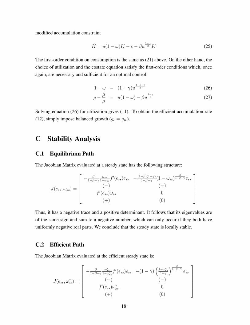
modified accumulation constraint
K = u(1minus ω)K minus cminus βu1minusγβ K (25)
The first-order condition on consumption is the same as (21) above On the other hand thechoice of utilization and the costate equation satisfy the first-order conditions which onceagain are necessary and sufficient for an optimal control
1minus ω = (1minus γ)u1minusβminusγβ (26)
ρminus micro
micro= u(1minus ω)minus βu
1minusγβ (27)
Solving equation (26) for utilization gives (11) To obtain the efficient accumulation rate(12) simply impose balanced growth (gc = gK)
C Stability Analysis
C1 Equilibrium Path
The Jacobian Matrix evaluated at a steady state has the following structure
J(ess ωss) =
minus β
1minusβminusγωss
1minusωssfprime(ess)ess minus (1minusβ)(1minusγ)
1minusβminusγ (1minus ωss)β
1minusβminusγ ess
(minus) (minus)
f prime(ess)ωss 0
(+) (0)
Thus it has a negative trace and a positive determinant It follows that its eigenvalues areof the same sign and sum to a negative number which can only occur if they both haveuniformly negative real parts We conclude that the steady state is locally stable
C2 Efficient Path
The Jacobian Matrix evaluated at the efficient steady state is
J(ess ωlowastss) =
minus β
1minusβminusγωlowastss
1minusωlowastssf prime(ess)ess minus(1minus γ)
(1minusωlowast
ss
1minusγ
) β1minusβminusγ
ess
(minus) (minus)
f prime(ess)ωlowastss 0
(+) (0)
18
again with negative trace and positive determinant so that the efficient steady state islocally stable too
D Proofs
Proposition 1 Consider that that using (5) and (11)
ulowast
u=
(1
1minus γ
) β1minusβminusγ
gt 1
since 0 lt γ lt 1minus β by assumption
Proposition 2 Showing that ωlowast gt ω is tantamount to showing that ln(1minusω)minusln(1minusωlowast) gt0 We have that
Dω equiv ln(1minus ω)minus ln(1minus ωlowast)
=1minus β minus γ
1minus γ[ln(1minus β minus γ)minus ln(1minus β)]minus ln(1minus γ)
andpartDω
partγ= minus β
(1minus γ)2[ln(1minus β minus γ)minus ln(1minus β)]
Hence the difference Dω increases in γ provided that the term in brackets is negative Thisis certainly true under 0 lt γ lt 1minus β since part ln(1minus β minus γ)partγ lt 0
Proposition 3 First observe that the first-order necessary condition for the choice ofutilization with the tax and subsidy solves for the firm-level utilization as
u =
(1minus ω1minus s
) β1minusβ
uγ
1minusβ (28)
Imposing the equilibrium condition u = u we find
usubs =
(1minus ω1minus s
) β1minusβminusγ
(29)
The comparison with equation (11) makes it clear that s = γ achieves the efficient utiliza-tion rate
To prove the second claim differentiate equations (29) and (28) (after taking logs for
19
simplicity) with respect to the subsidy s to see that
part lnusubs
parts=
β
1minus β minus γ1
1minus sgtpart lnu
parts=
β
1minus β1
1minus slArrrArr γ isin (0 1minus β)
The size of the fiscal multiplier m can be recovered by dividing the aggregate response bythe individual response We have that
m =1minus β
1minus β minus γ=
1
1minus γ1minusβ
Conflict of InterestThe authors declare that they have no conflict of interest
References
Auerbach P and Skott P 1988 lsquoConcentration Competition and Distribution ndash A Cri-tique of the Theories of Monopoly Capitalrsquo International Review of Applied Economics
2 (1) 42ndash61
Cooper R 1999 Coordination Games Cambridge UK Cambridge University Press
Cornwall J and Setterfield M (2002) A neo-Kaldorian perspective on the rise and declineof the golden age In M Setterfield (ed) The Economics of Demand-Led Growth Chal-
lenging the Supply Side Vision of the Long Run pp 67ndash86 Cheltenham UK EdwardElgar
Dumenil G and Levy D 1999 lsquoBeing Keynesian in the Short Term and Classical in theLong Term the Traverse to Classical Long-Term Equilibriumrsquo Manchester School 67(6) 684ndash716
Fatas A 2019 lsquoFiscal Policy Potential Output and the Shifting Goalpostsrsquo Paper pre-sented at the Euro 20 academic conference organized by the IMF and Bank of IrelandAvailable at httpsfacultyinseadedufataseuro20pdf
Foley D K Michl T R and Tavani D 2019 Growth and Distribution Second Edition
Cambridge MA Harvard University Press
Foley D K 2003 lsquoEndogenous Technical Change with Externalities in a Classical GrowthModelrsquo Journal of Economic Behavior and Organization 52 167ndash189
20
Foley D K 2016 lsquoKeynesrsquo Microeconomics of Output and Labor Marketsrsquo In BernardL and Nyambuu eds Dynamic Modeling Empirical Macroeconomics and Finance
Essays in Honor of Willi Semmler Springer pp 183ndash194
Goodwin R 1967 lsquoA Growth Cyclersquo In Socialism capitalism and economic growthCambridge UK Cambridge University Press
Greenwod J Hercowitz Z and Huffman G 1988 lsquoInvestment Capacity utilizationand the Real Business Cyclersquo American Economic Review 78 (3) 402ndash417
Jones C I 1995 RampD-Based Models of Economic Growth Journal of Political Economy
103 (4) 759ndash784
Jones C I 1999 Growth With or Without Scale Effects American Economic Review
(Papers and Proceedings) 89 (2) 139ndash144
Julius A J 2005 Steady State Growth and Distribution with an Endogenous Direction ofTechnical Change Metroeconomica 56 (1) 101ndash125
Kaldor N 1956 lsquoAlternative theories of distributionrsquo Review of Economic Studies 23 (2)83ndash100
Kaldor N 1961 lsquoCapital accumulation and economic growthrsquo In F A Lutz and D CHague (eds) The Theory of Capital New York NY St Martins Press
Kennedy C (1964) Induced bias in innovation and the theory of distribution Economic
Journal 74 (295) 541ndash547
Keynes J M 1936 The General Theory of Employment Interest and Money LondonMacMillan
Michl T R 2009 Capitalists Workers and Fiscal Policy Cambridge MA Harvard Uni-versity Press
Michl T R 2017 ldquoProfit-led Growth and the Stock Marketrdquo Review of Keynesian Eco-
nomics 5 (1) 61ndash77
Michl T R and Oliver K M 2019 ldquoCombating Hysteresis with Output Targetingrdquo Re-
view of Keynesian Economics 7 (1) 6ndash27
Naastepad CWM (2006) Technology demand and distribution A cumulative growthmodel with an application to the Dutch productivity growth slowdown Cambridge Jour-
nal of Economics 30 403ndash434
21
Petach L and Tavani D 2019 lsquoNo one is Alone Strategic Complementarities Capac-ity Utilization Growth and Income Distributionrsquo (April 17 2019) Available at SSRNhttpsssrncomabstract=3123149
van der Ploeg R 1985 Classical Growth Cycles Metroeconomica 37 (2) 221-230
Rada C (2007) Stagnation or transformation of a dual economy through endogenousproductivity growth Cambridge Journal of Economics 31 711ndash740
Romer P (1987) Growth Based on Increasing Returns Due to Specialization American
Economic Review 77 56ndash62
Setterfield M 2018 ldquoLong-run Variation in Capacity Utilization in the Presence of a FixedNormal Raterdquo Cambridge Journal of Economics 43 (2) 443ndash463
Shah and Desai M 1981 Growth Cycles with Induced Technical Change EconomicJournal 91 1006ndash1010
Skott P 1989 Conflict and Effective Demand in Economic Growth Cambridge UK Cam-bridge University Press
Skott P 2010 lsquoGrowth Instability and Cycles Harrodian and Kaleckian Models of Ac-cumulation and Income Distributionrsquo In M Setterfield Ed Handbook of Alternative
Theories of Economic Growth London UK Edward Elgar
Skott P 2012 lsquoTheoretical and Empirical Shortcomings of the Kaleckian InvestmentFunctionrsquo Metroeconomica 63 (1) 109-138
Skott P 2017 ldquoWeaknesses of Wage-led Growthrdquo Review of Keynesian Economics 5 (3)336-359
Tavani Dand Zamparelli L 2015 lsquoEndogenous Technical Change Employment andDistribution in the Goodwin Model of the Growth Cyclersquo Studies in Nonlinear Dynamics
and Econometrics 19 (2) 209-226
Tavani D and Zamparelli L 2017 Endogenous Technical Change in Alternative Theo-ries of Growth and Distribution Journal of Economic Surveys 31 (5) 1272-1303
Tavani D and Zamparelli L 2017 lsquoGrowth Income Distribution andthe Entrepreneurial Statersquo Journal of Evolutionary Economics 2018httpsdoiorg101007s00191-018-0555-7
22
Taylor L Foley DK Rezai A (2018) Demand drives growth all the way Good-win Kaldor Pasinetti and the Steady State Cambridge Journal of Economics bey045httpsdoiorg101093cjebey045
Verdoorn PJ (1949) Fattori che regolano lo sviluppo della produttivita del lavoroLrsquoIndustria 1 3-10
23
Introduction
Basic Elements of the Model
Equilibrium Utilization and Accumulation
The Dynamical System
Steady State
Stability Analysis
Welfare and Policy
Decentralization
Extension Endogenous Labor Productivity Growth
Conclusion
The Capitalists Optimization Problem
The Efficient Solution
Stability Analysis
Equilibrium Path
Efficient Path
Proofs
1 Introduction
One of the most debated questions in alternative macroeconomics regards whether demandpolicies have permanent or merely transitory effects While Kaleckian economists haveargued that demand matters even in the long run both economists operating within otherKeynesian traditionsmdashsuch as Harrodians (eg Skott 1989 2010 2012 2017)mdashas wellas Classical economists (Dumenil and Levy 1999) argue that long-run output growth isconstrained by the so-called natural rate Moreover it is argued the long-run rate of uti-lization of installed capacity which proxies for effective demand in these frameworks mustnecessarily be exogenous With fully adjusted exogenous utilization and growth fixed atthe natural rate many of the central results of canonical Kaleckian models appear to be injeopardy the paradox of thrift the paradox of costs and the relevance of effective demandin the long-run may no longer hold The latter is especially concerning given its centralityfor (post-) Keynesian economics
This is not just an academic dispute considerations about lackluster aggregate demandhave been especially relevant in the aftermath of the Great Recession and the sluggishrecovery that followed in most of the worldrsquos advanced economies Figure 1 plots realGDP in the United States against the Congressional Budget Office estimates of potentialoutput in 2007 and the revised CBO estimates in 2017 The downward revision of potentialoutput points to the presence of considerable slack capacity in the US economy over adecade after the Great Recession ended (Fatas 2019)
Figure 1 US Real GDP (billions of chained US dollars black) vs the CBO estimates ofpotential GDP in 2007 (gray) and the CBO estimates of potential GDP in 2017 (dashed)Source Congressional Budget Office
2000 2005 2010 2015
12000
13000
14000
15000
16000
17000
18000
RealGDP
Such observations point to the question if one takes the objections of the Harrodian
2
and Classical perspectives seriously is it necessary to abandon hope for the possibility ofa meaningful role for effective demand in the medium-to-long run Our answer is noWhile the Classical demarcation limiting the effectiveness of demand policy to the short-runmdashwhich has led Dumenil and Levy (1999) to a description of the world as ldquoshort-runKeynesian long-run Classicalrdquomdashmay be analytically useful it is unlikely to hold true inactually existing capitalist economies Michl (2017) then points out that a key task foralternative economic theories is to engage in what theologians call ldquoirenicsrdquo or the processof reconciling conflicting doctrines in order to paint a more realistic picture of the spacecapitalist economies actually inhabitmdasha space which undoubtedly combines elements ofboth the Classical and Keynesian visions (p74)
Our task in this paper is thus to develop a micro-to-macro fully Classical model fea-turing an explicit dynamic choice of utilization at the firm level in order to illustrate amechanism that may give rise to lackluster economic performance as an equilibrium out-come Our argument is that if firms formulate beliefs about the state of the economy whenselecting their own level of capacity utilization then demand policies can certainly affectthe level of economic activity in the long-runmdashdespite growth being fixed at the naturalrate The inclusion of beliefs in our model harkens back to the central role that expecta-tions play in the process of employment determination envisioned by Keynes (1936) in The
General Theory ldquo[T]odayrsquos employment can be correctly described as being governed bytodayrsquos expectations taken in conjunction with todayrsquos capital equipmentrdquo (p50) Despitethe central role afforded to the process of expectations-formation by Keynes (1936) rela-tively little effort has been put forth in formalizing beliefs in (post-) Keynesian models withan explicit microeconomic structure Borrowing insights from the literature on coordina-tion games (Cooper 1999) we will show that firm-level beliefs about economic activitycan be captured in a simple way by including (expectations about) the aggregate utilizationrate in the economy as a signal for the current level of effective demand To gain intuitionconsider the following scenario Suppose an individual firm operating at its desired utiliza-tion expects other firms to increase production because the economy is picking up steamIf such beliefs about other firmsrsquo behavior did not have an effect on the firmrsquos own choicethen it must be true that the firm has already maximized its profits and has no incentiveto deviate from the corresponding desired rate of utilization But this cannot be the casebecause the firm can in fact increase its profits by simply utilizing more its capacity in lightof its beliefs about the economy Thus it must be that beliefs enter the choice of utilizationat the firm level
Following Petach and Tavani (2019) we operationalize this assumption extending theKeynesian notion of the user cost of capitalmdashthe opportunity cost incurred by firms when-
3
ever they choose to undertake productionmdashto a more general adjustment cost of operatingequipment First the concept of user cost as outlined by Keynes (1936) is forward-lookingldquo[I]t is the expected sacrifice of future benefit involved in present use which determines theamount of user cost and it is the marginal amount of this sacrifice which determines his(sic) scale of productionrdquo (p70) In other words the user-cost of capital does not merelydepend on the firmrsquos current own-rate of utilization but intertemporal considerations areat play when the choice of utilization is made Thus our rendition of the user cost has anindividual component and it is increasing and convex in the firmrsquos own utilization rate andis embedded in a forward-looking optimization problem Greenwood et al (1988) havealready argued that this individual component captures in a simple but faithful way thefirm-level trade-offs pointed out by Keynes
Second we argue that the cost of utilizing equipment also entails an outward-looking
component which depends on the individual firmrsquos beliefs about the behavior of the aggre-gate economy and motivates our extension of the user cost into a more general adjustmentcost function Thus we introduce a dependence of the cost of utilization on the aggregateutilization rate in the firmrsquos sectormdashor in the economy in the representative firm casemdashinorder to capture the individual firmrsquos incentives to adjust its production given changes inexpectations Specifically we propose a specification of the adjustment cost function wherethe marginal adjustment cost is declining in the average rate of utilization in the economyUnder empirically-sound restrictions (see the results in Petach and Tavani 2019) this for-malization delivers strategic complementarities among firms the desired rate of utilizationat the firm level increases in aggregate utilization it is endogenous to demand in otherwords This feature will produce an equilibrium utilization rate and therefore an equi-librium level of economic activity that is inefficiently low firms will keep some sparecapacity in order to react to the possibility of increased aggregate demand in the economywhile at the same time engaging in the accumulation process
The result can then be used in order to draw policy implications With exogenoustechnical changemdashthe most common specification of technological progress in Harrodianmodelsmdashthe economyrsquos growth rate is exogenously fixed at the natural rate n Accord-ingly there are no growth effects of demand policies However underutilization impliesthat spending policies have positive level effects both on output per worker and the share oflabor The latter will increase in response to spending policies that boost economic activityThus the conclusions of this analysis are that demand matters even in the long run bothfor the level of economic activity and the labor share
In addition to analyzing the effects of demand policies on an economyrsquos balanced growthpath we also consider the implications of incorporating adjustment costs and a strategic
4
choice of capacity utilization for the Goodwin (1967) model whose steady state is virtu-ally identical to Kaldor (1956) but whose focus is on the endless distributive cycle betweenthe employment rate and the labor share The literature has identified four main channelsthrough which the perpetual cycle can be resolved in the long run (i) capitallabor substi-tution along a neoclassical production function (van der Ploeg 1985) (ii) an endogenouslabor-augmenting bias of technical change (Shah and Desai 1981 Foley 2003 Julius2005) (iii) endogenous labor-augmenting innovation financed out of profits (Tavani andZamparelli 2015) and (iv) differential tax rates on capital versus labor incomes in modelswith public infrastructure (Tavani and Zamparelli 2018) In all of these cases the sym-metry in the bargaining positions between capital and labor which is responsible for theendless Goodwin growth cycle (Shah and Desai 1981) is broken in favor of the formerWe show in this paper that the choice of utilization implied by our model acts in the sameway namely turning the resulting steady state from the Goodwin center to a stable focusEssentially the possibility of varying the rate of utilization is analogous to changing thetechnique of production in response to factor shares which is at the heart of the stabilizingchannels discussed in the literature
Finally we also analyze an extension of the model featuring endogenous technicalchange in the form of a Verdoorn law (Verdoorn 1949) the growth rate of labor pro-ductivity depends on the accumulation rate However as it is well-known in the literaturea Verdoorn law delivers a semi-endogenous long-run growth rate it is derived within themodel but is constrained by exogenous parameters such as the growth rate of the labor forceand the Verdoorn pass-through (see the discussion in Tavani and Zamparelli 2017) Differ-ently from the exogenous technical change model however expansionary fiscal policy thatfosters utilization will have a temporary growth effect in addition to its permanent leveleffect Therefore this version of the model shows that demand policies translate mean-ingfully into changes in the growth rate via their impact on the accumulation rate alongthe transition to balanced growth Thus the paper offers one explanation for why tempo-rary demand shocks have permanent level effects under exogenous growth or temporarygrowth effects under endogenous labor-augmenting technical change and offers an addi-tional contribution to the analysis of hysteresis in Classical and Keynesian growth modelsby Setterfield (2018) Michl and Oliver (2019)
2 Basic Elements of the Model
Consider a competitive capitalist firm in a closed economy and assume away the gov-ernment for now Let the firmrsquos production possibilities be summarized by the Leontief
5
technology Y = minuKAL where Y is the firmrsquos output homogeneous with capitalstock K so that we can normalize its price to one u denotes the rate of capacity utiliza-tion L stands for labor A is the current stock of labor-augmenting technologies assumedto grow at the constant rate gA gt 0 in the benchmark model so that the analysis is asclose as possible to baseline Harrodian models such as Skott (1989) and the long-run out-putcapital ratio B is normalized to one for simplicity Time is continuous Maximizingprofits requires to set uK = AL which solves for labor demand L = uKA If the firmpays the same real wage w to each worker the share of wages in output will be equal tothe unit labor cost ω equiv wA Further let the labor force N ge L grow at the constant raten gt 0 Thus the employment rate in the economy e will be equal to LN = uK(AN)
Our main hypothesis is that operating capital equipment entails an adjustment cost λwhich would not be incurred if machinery remained idle (Keynes 1936) First and tocapture the user cost we assume that the adjustment cost increases more than propor-tionally with the firmrsquos own utilization rate u denoting partial derivatives by subscriptsλu gt 0 λuu gt 0 Greenwood et al (1988) have noted that this specification formalizesthe Keynesian effects played by the lsquomarginal efficiency of investmentrsquo and the Keynesiannotion of user cost for the individual firm Second we capture the strategic nature of thechoice of utilization by postulating that the adjustment cost also responds to the firmrsquos be-liefs about the utilization chosen by other firms as captured by u the average utilizationrate We assume that u has a negative impact on the marginal adjustment cost λuu lt 0This assumption implies that the marginal benefit of increasing own utilization increases inthe firmrsquos beliefs about aggregate utilization and is required to generate a strategic com-plementarity which is central in our contribution Petach and Tavani (2019) have offeredstrong and robust empirical support for this assumption using a panel of state-by-sectordata for the United States To sharpen our conclusions we specify a log-linear user costfunction as in Petach and Tavani (2019)
λ(u u) = βu1β uminus
γβ β isin (0 1) γ isin [0 1minus β) (1)
The size of the parameter γ determines the extent to which beliefs about other firmsrsquo be-havior are relevant for the firm choice The special case γ = 0 corresponds to the isolatedfirms case where the choices made by other firms are irrelevant while γ 6= 0 implies astrategic environment in which beliefs matter Further under 0 lt γ lt 1minus β the choice ofutilization generates a (weak) strategic complementarity which will result in a unique non-trivial long-run equilibrium utilization in the model The estimates in Petach and Tavani(2019) strongly support the above parametric restriction that 0 lt γ lt 1minus β
6
In line with the basic Classical and Post Keynesian literature we assume that only profit-earning (capitalist) households save in order to accumulate capital stock However whilein most of the literature capitalists save a constant fraction of their profit incomes at alltimes we follow Foley Michl and Tavani (2019) in assuming that capitalist householdsare forward-looking in their consumption accumulation and utilization decisions Thisassumption is made here in order to rule out any potential lsquoinefficiencyrsquo result implied by alimited planning horizon or by lsquorule of thumbrsquo behavior such as saving the same fractionof income at all times1 Here the capitalist household discounts the future at a constantrate ρ gt 0 derives instantaneous logarithmic utility from its per-period consumption flowdenoted by c(t) and has perfect foresight on the entire planning horizon t isin [sinfin) Finallyassume that there is no independent investment demand function so that capitalist savingsare immediately invested at all times The accumulation constraint omitting the time-dependence for notational simplicity is
K = (1minus ω)uK minus cminus λ(u u)K (2)
Note that increasing the own rate of utilization raises the capitalistrsquos revenues (1minus ω)uKbut also increases the adjustment cost λ(u u) given average utilization As shown in Ap-pendix A the solution to a simple control problem delivers the firm-level choice of ca-pacity utilization as a decreasing function of the labor share while increasing in averageutilization as per equation (3) below The firm-level choice of utilization is equivalent to abest-response function in the game-theoretic sense or a reaction function in Cournot-stylemodels
u(ω u) = (1minus ω)β
1minusβ uγ
1minusβ (3)
Figure 2 displays the behavior of the best-response function in relation to the aggregateutilization rate The intuition for the inverse dependence on the labor share is that anincrease in the latter reduces revenues everything else equal the firm can then cut back onits utilization in order to reduce the user cost of capital On the other hand an increasein aggregate utilization reduces the own marginal adjustment cost everything else equalthus rising the marginal profits that can be made by utilizing more a firmrsquos own installedcapacity the firm can increase utilization up to the point where the marginal benefit ofdoing somdashgiven by (1 minus ω)Kmdashis equal to the marginal user cost λu(u u)K for a givenaverage utilization rate Finally given that the firmrsquos beliefs about aggregate utilizationrepresent expectations about the overall economic activity in the economy the dependence
1Similar reasoning applies to the assumption of competitive firms the results of the model do not dependon slow price adjustments as Skott (2017) has argued to be the case in neo-Kaleckian growth models
7
on average utilization can be thought of as capturing the endogeneity of the firmrsquos desiredrate of utilization to demand Appendix A also shows that the growth rate of consumptionfor the typical capitalist householdmdashwhich describes the household-level saving rulemdashsatisfies
gc equivc
c= (1minus ω)
11minusβ u
γ1minusβ minus ρ (4)
Figure 2 Equilibrium vs efficient utilization rates
U
u = u
U u
u
3 Equilibrium Utilization and Accumulation
An equilibrium growth path is a sequence of quantities c(t) u(t) u(t) k(t)tisin[sinfin) thatsolve the capitalistrsquos control problem given the path for the labor share ω(t)tisin[sinfin) andsuch that u(t) = u(t) for all t The latter requirement requires firms to best-respond to otherfirmsrsquo choices similarly to the notion of a Nash equilibrium Omitting the time notationfor simplicity the equilibrium rate of utilization is easily found as
u(ω) = (1minus ω)β
1minusβminusγ (5)
and is inversely related to the labor share since 1minusβminusγ gt 0 by assumption The intuitionis simple a higher wage share lowers the firmrsquos profits and thus the resources available foraccumulation But the firm can offset the higher wage costs by utilizing less its plants thusreducing the user cost
We can then obtain the equilibrium growth rate by using the condition u = u andimposing balanced growth so that consumption and capital stock grow at the same rate
8
gc = gK = g We haveg = (1minus β)(1minus ω)
1minusγ1minusβminusγ minus ρ (6)
where the first term in the right-hand-side of (6) is the profit rate net of the adjustmentcost Further because of the equilibrium condition u = u the equilibrium adjustment costλ(uu) reduces to the pure user cost of capital ie depreciation
4 The Dynamical System
First consider the economyrsquos share of labor ω = wA Its growth rate will be givenby the difference between the growth rate of the real wage and the growth rate of laborproductivity Following Goodwin (1967) assume that real wages obey a version of thePhillips curve ww = f(e) such that fe gt 0 fee gt 0 In particular we impose f(e) =
ηe1δ η gt 0 δ isin (0 1) Hence the labor share evolves according to
ω
ω= f(e)minus gA (7)
Next consider the employment rate e = uK(AN) Logarithmic differentiation gives
e
e= gK + gu minus (gA + n)
Differentiating (5) we obtain the growth rate of utilization as
u
uequiv gu = minus β
1minus β minus γ
(ω
1minus ω
)ω
ω(8)
so that using the real-wage Phillips curve (7) and the accumulation rate from (6) we find
e =
(1minus β)(1minus ω)
1minusγ1minusβminusγ minus β
1minus β minus γ
(ω
1minus ω
)[f(e)minus gA]minus (ρ+ gA + n)
e (9)
41 Steady State
A steady state is a pair (ωss ess) so that ω = e = 0 Notice that the steady state value ofutilization is uniquely pinned down by the steady state labor share given the equilibriumcondition u = u that delivers equation (5) above The steady state value of the employmentrate is readily found by setting ω = 0 in (7)
ess =
(gAη
)δ(E)
9
The steady state employment rate is fully exogenous because of the exogenous nature oftechnological change in the model On the other hand the steady state value for the laborshare can be solved for in closed form once noting that f(ess) = gA in setting the right-handside of equation (9) equal to zero By so doing we find
1minus ωss =
(ρ+ n+ gA
1minus β
) 1minusβminusγ1minusγ
(Ω)
We can now state a first result of this analysis namely the dependence of steady stateutilization on the capitalist saving rate as a proposition
Proposition 1 The steady state desired utilization rate uss increases in the discount rate ρ
Since the latter reduces savings in the economy the paradox of thrift holds in this model
To prove this result use (5) to solve for the steady state utilization rate as
uss =
(ρ+ n+ gA
1minus β
) β1minusγ
(10)
and partusspartρ gt 0 The result is remarkable because even without an explicit investmentfunction this model delivers a version of the Keynesian paradox of thrift A higher valueof the discount rate ρ reduces the long-run capitalistsrsquo saving the corresponding increasein long-run aggregate consumption can be met by increasing utilization and therefore thesteady-state level of economic activity
42 Stability Analysis
Appendix C shows that unlike the original Goodwin (1967) long-run the steady state ofthis model is locally stable Thus the explicit choice of capacity utilization is an additionalway of breaking the symmetric bargaining positions between capital and labor resolvingthe distributive conflict in the long run (Shah and Desai 1981 van der Ploeg 1985) Figure3 shows the ω = 0 nullcline which is vertical corresponding to the steady state employmentrate ess and is the same at both the equilibrium and the efficient solution and plots the e = 0
nullcline in red The latter is downward sloping and so will be the nullcline correspondingto the efficient growth path as differentiation of the expression in braces in (9) and (13) willshow Notice also that convergence to the steady state is not monotonic the employmentrate which is the forward-looking variable in this model overshoots before convergingto its long-run value In this respect explicit demand shocks (see below) will determinesome short-run cyclical behavior of the system before a new steady state is achieved A
10
time-series plot is displayed in Figure 4
Figure 3 Phase Diagram equilibrium nullclines (red) and efficient e = 0 nullcline (blue)and dynamic trajectories converging to the equilibrium (dotted gray) as opposed to theefficient (solid black) steady state The vector field plot refers to the equilibrium path
ω
ω
ω
ω
5 Welfare and Policy
An interesting feature of this economy is that so long as a (weak) strategic complementar-ity is presentmdashthat is so long as 0 lt γ lt 1 minus βmdashit will generally operate with excesscapacity in equilibrium while at the same time accumulating capital stock To see this letus introduce a benevolent planner solving the accumulation problem under the additionalconstraint that u = u at all times Appendix B proves the following result
Proposition 2 Let γ isin (0 1minus β) Then the efficient choice of utilization is
ulowast(ω) =
(1minus ω1minus γ
) β1minusβminusγ
(11)
and is strictly greater than its decentralized counterpart (5)
Notice that the parameter γ generates a multiplier effect the larger the extent to which firmbeliefs matter the higher the socially-coordinated utilization rate relative to the equilibriumrate Absent a role for beliefs γ = 0 the equilibrium rate and the socially-coordinated rate
11
Figure 4 Equilibrium vs efficient trajectories for the employment rate and the labor share
ω
ω
() ()
coincide This result is important for two reasons first as long as firms operate withina strategic context they will find it profit-maximizing to keep accumulating capital stockeven though their capacity is not fully utilized Second the result shows that the individualcomponent of the user cost function is not sufficient to generate underutilization the pres-ence of a strategic environment where firmsrsquo decisions are affected by other firmsrsquo choicesis necessary for the economy to operate below full capacity in equilibrium Figure 2 showsthe equilibrium as opposed to the efficient utilization rate in this model Using (11) we canthen solve for the efficient accumulation rate as
glowast =
(1minus ω1minus γ
) 1minusγ1minusβminusγ
(1minus β minus γ)minus ρ (12)
which can then be used in order to track the evolution of employment along the efficientgrowth path The law of motion for the labor share does not change therefore the efficientsteady state value for the employment rate is still given by equation (E) above Instead theevolution of employment over time modifies to2
e
e= (1minusβminus γ)
(1minus ω1minus γ
) 1minusγ1minusβminusγ
minus β
1minus β minus γ
(ω
1minus ω
)[f(e)minus gA]minus (ρ+ gA +n) (13)
2Interestingly the growth rate of utilization obtained log-differentiating (11) is identical to the correspond-ing equilibrium growth rate as per equation (8)
12
Proceeding as before then we find the steady state labor share at the efficient growth pathas the solution to
1minus ωlowastss = (1minus γ)
(ρ+ gA + n
1minus β minus γ
) 1minusβminusγ1minusγ
(Ωlowast)
The Appendix then proves the following result
Proposition 3 Let 1minus β gt γ gt 0 Then ωlowastss gt ωss
Petach and Tavani (2019) have estimated equation (3) through a series of empirical modelsusing state-by-sector US data with the aim of assessing the extent of strategic complemen-tarities Those results provide strong evidence regarding the empirical bite of our argumentThe point estimates for the main parameters of interest γ and β are highly significant androbust to different model specifications and fully in line with the theoretical restrictionsneeded for Proposition 3 to hold Thus the analysis provides strong reasons to believe thatdemand policies can be used in order to improve the workersrsquo distributional position in theeconomy We carry a simple exercise to this aim in the next Section
51 Decentralization
Let us introduce a government authority that subsidizes the user cost at a rate s andmdashforsimplicitymdashtaxes capitalist income lump-sum by an amount τ while running a balancedbudget τ = sλ(middot)K at all times3 The capitalist householdsrsquo budget constraint modifies asfollows
K = (1minus ω)uK minus τ minus cminus λ(u u)K(1minus s) (14)
Solving the corresponding optimal control problem we have the following result provenin the Appendix
Proposition 4 (i) The subsidy that decentralizes the efficient utilization rate and labor
share is equal to γ which governs the extent of strategic complementarities (ii) The ag-
gregate response to an increase in s is always greater than the individual firmrsquos response
(iii) The resulting lsquofiscal multiplierrsquo is equal to 11minus γ
1minusβ
6 Extension Endogenous Labor Productivity Growth
The reason why the baseline model delivers only level effects of demand policies has to befound in the assumption of exogenous technical change Since the growth rate of labor pro-
3Setting τ = 0 amount to impose a deficit-financed user cost subsidy
13
ductivity is fixed at its exogenous rate gA there are necessarily no growth effects of spend-ing policies aimed at implementing the efficient rate of utilization However economistsworking within alternative traditions (Cornwall and Setterfield 2002 Naastepad 2006Rada 2007 Taylor et al 2018) have long emphasized the possibility of demand shocksaffecting labor productivity growth here we show that a simple extension of the modeldelivers transitory effects of demand shocks on the growth rate of labor productivity in ad-dition to its permanent level effects In line with the contributions mentioned above assumethat labor productivity growth follows a version of Verdoornrsquos law (Verdoorn 1949)4
gA = φgK φ isin (0 1) (15)
While labor productivity growth is endogenous its long run value is anchored by the bal-anced growth condition gA + n = gK so that in the long run we end up with a semi-
endogenous growth rate the growth rate is determined within the model but independentof policy (Jones 1995 1999) In fact we have
gK =n
1minus φ gA =
φn
1minus φ (16)
Importantly however Verdoornrsquos law creates transitory effects of demand policy on laborproductivity growth Both the efficient and the equilibrium accumulation paths converge tothe same growth rate in (16) but the efficient path involves a growth rate of labor productiv-ity that converges from above relative to the equilibrium path as shown in Figure 55 Thisresult points to the additional welfare effects of demand policiesmdashgiven by the integral ofthe distance between the two curvesmdashalong the transition to balanced growth Thus evenif it only impacts the level of output in the long-run demand policy may nonetheless havepermanent positive effects on social welfare via its impact on productivity growth duringthe transition to the steady-state
For completeness let us evaluate the steady state of the extended model Incorporatingequation (15) into the dynamical system (7)-(9) and solving for the steady state income
4In the conventional AK-growth literature the stock of labor-augmenting technologies depends on theaggregate capital stock A = ζKφ ζ gt 0 φ isin (0 1) through a learning-by-doing externality Log-differentiation of this expression gives equation (15) See Romer (1987)
5The figure uses the same parameter calibration as the baseline model plus a value of φ that ensures along-run growth rate of 3 It is displayed for illustrative purposes and it is not meant to argue that demandpolicies can boost labor productivity growth up to over 12 as a literal interpretation of the figure wouldsuggest
14
Figure 5 Equilibrium (gray) vs efficient (black) path of labor productivity growth givenan initial condition on the labor share with a Verdoorn effect
shares and employment rate corresponding to an equilibrium path gives
1minus ωss =
[n+ ρ(1minus φ)
(1minus β)(1minus φ)
] 1minusβminusγ1minusγ
(17)
ess =
[φn
η(1minus φ)
]δ(18)
The efficient path solves for the same long-run employment rate as (18) but delivers thefollowing long-run distribution of income
1minus ωlowastss = (1minus γ)
[n+ ρ(1minus φ)
(1minus β minus γ)(1minus φ)
] 1minusβminusγ1minusγ
(19)
and Proposition 3 holds in this version of the model too6
7 Conclusion
In this paper we have offered one potential resolution to what Michl (2017) calls the ldquodis-cord in the marriage of Classical and Keynesian economics that defines modern heterodoxmacroeconomicsrdquo (p77) Namely the discord caused by conflicting claims about the re-lationship of effective demand to long-run growth Our solution relies on the introduction
6The proof goes along the same lines as Proposition 3
15
of beliefs into the firmrsquos choice of utilization in an otherwise Classical long-run model ofgrowth and distribution Firmsrsquo beliefs are modeled via an adjustment cost function andin particular a declining marginal adjustment cost in the economy-wide rate of utilizationUnder reasonable and empirically-supported restrictions on parameter values we showedthat this specification is sufficient to generate a desired utilization rate at the firm level thatincreases in aggregate utilization As a result we are able to carve out a role for demandpolicy in our model Even though growth is fixed at the natural rate spending policieswill always have level effects on long-run output because equilibrium utilization is belowthe efficient level We then provided a dynamic extension of the model to study the im-plications of a firm-level choice of utilization in the Goodwin (1967) growth cycle thechoice of utilization resolves the distributive conflict in favor of the capitalist class alteringthe steady-state of the Goodwin model into a stable focus However the model exhibitsovershooting of the employment rate before it reaches equilibrium consistent with Keynes(1936) Finally we have shown that with a Verdoorn (1949) effect on labor productivitygrowth demand shocks can temporarily impact the rate of growth via their impact on theaccumulation rate
As a final observation the focus of this paper is on the effectiveness of fiscal policy inlabor-constrained economies Our analysis points to the relevance of coordination failuresin devising a role for spending policies that will increase economic activity and the laborshare despite equilibrium utilization being profit-led in the usual Post-Keynesian jargonEven though our model is purely supply-side we showed that (i) the paradox of thriftholds (ii) spending policies have generally multiplier effects and (iii) are generally labor-friendly Our conclusions will only be reinforced in an analysis that includes a demand-driven determination of economic activity
A The Capitalistsrsquo Optimization Problem
Suppose that the representative capitalist household has logarithmic preferences over con-sumption streams and discounts the future at a constant rate ρ gt 0 Then the household
16
solves
Given u(t) ω(t)forallt
Choose c(t) u(t)tisin[sinfin) to maxint infins
expminusρ(tminus s) ln c(t)dt
s t K(t) = [1minus ω(t)]u(t)K(t)minus c(t)minus λ[u(t) u(t)]K(t)
K(s) equiv Ks gt 0 givenlimtrarrinfin
expminusρ(tminus s)K(t) ge 0
(20)Observe first that the problem stated in (20) involves a strictly concave objective function tobe maximized over a convex set Thus the standard first-order conditions on the associatedcurrent-value Hamiltonian
H = ln c+ micro[u(1minus ω)K minus cminus λ(u u)K]
will be necessary and sufficient for an optimal control They are
Solving (22) for the rate of utilization under the specific functional form (1) gives (3) Toobtain the Euler equation for consumption differentiate (21) with respect to time and use(21) and (23) to get
gc equivc
c= (1minus ω)u(ω u)minus λ[u(ω u)] + ρ
Using both (3) and (1) while imposing a balanced growth path where consumption andcapital stock grow at the same rate gives (4)
B The Efficient Solution
A benevolent social planner solves the accumulation problem under the additional con-straint that u = u at all times Accordingly the control problem (20) is solved under the
17
modified accumulation constraint
K = u(1minus ω)K minus cminus βu1minusγβ K (25)
The first-order condition on consumption is the same as (21) above On the other hand thechoice of utilization and the costate equation satisfy the first-order conditions which onceagain are necessary and sufficient for an optimal control
1minus ω = (1minus γ)u1minusβminusγβ (26)
ρminus micro
micro= u(1minus ω)minus βu
1minusγβ (27)
Solving equation (26) for utilization gives (11) To obtain the efficient accumulation rate(12) simply impose balanced growth (gc = gK)
C Stability Analysis
C1 Equilibrium Path
The Jacobian Matrix evaluated at a steady state has the following structure
J(ess ωss) =
minus β
1minusβminusγωss
1minusωssfprime(ess)ess minus (1minusβ)(1minusγ)
1minusβminusγ (1minus ωss)β
1minusβminusγ ess
(minus) (minus)
f prime(ess)ωss 0
(+) (0)
Thus it has a negative trace and a positive determinant It follows that its eigenvalues areof the same sign and sum to a negative number which can only occur if they both haveuniformly negative real parts We conclude that the steady state is locally stable
C2 Efficient Path
The Jacobian Matrix evaluated at the efficient steady state is
J(ess ωlowastss) =
minus β
1minusβminusγωlowastss
1minusωlowastssf prime(ess)ess minus(1minus γ)
(1minusωlowast
ss
1minusγ
) β1minusβminusγ
ess
(minus) (minus)
f prime(ess)ωlowastss 0
(+) (0)
18
again with negative trace and positive determinant so that the efficient steady state islocally stable too
D Proofs
Proposition 1 Consider that that using (5) and (11)
ulowast
u=
(1
1minus γ
) β1minusβminusγ
gt 1
since 0 lt γ lt 1minus β by assumption
Proposition 2 Showing that ωlowast gt ω is tantamount to showing that ln(1minusω)minusln(1minusωlowast) gt0 We have that
Dω equiv ln(1minus ω)minus ln(1minus ωlowast)
=1minus β minus γ
1minus γ[ln(1minus β minus γ)minus ln(1minus β)]minus ln(1minus γ)
andpartDω
partγ= minus β
(1minus γ)2[ln(1minus β minus γ)minus ln(1minus β)]
Hence the difference Dω increases in γ provided that the term in brackets is negative Thisis certainly true under 0 lt γ lt 1minus β since part ln(1minus β minus γ)partγ lt 0
Proposition 3 First observe that the first-order necessary condition for the choice ofutilization with the tax and subsidy solves for the firm-level utilization as
u =
(1minus ω1minus s
) β1minusβ
uγ
1minusβ (28)
Imposing the equilibrium condition u = u we find
usubs =
(1minus ω1minus s
) β1minusβminusγ
(29)
The comparison with equation (11) makes it clear that s = γ achieves the efficient utiliza-tion rate
To prove the second claim differentiate equations (29) and (28) (after taking logs for
19
simplicity) with respect to the subsidy s to see that
part lnusubs
parts=
β
1minus β minus γ1
1minus sgtpart lnu
parts=
β
1minus β1
1minus slArrrArr γ isin (0 1minus β)
The size of the fiscal multiplier m can be recovered by dividing the aggregate response bythe individual response We have that
m =1minus β
1minus β minus γ=
1
1minus γ1minusβ
Conflict of InterestThe authors declare that they have no conflict of interest
References
Auerbach P and Skott P 1988 lsquoConcentration Competition and Distribution ndash A Cri-tique of the Theories of Monopoly Capitalrsquo International Review of Applied Economics
2 (1) 42ndash61
Cooper R 1999 Coordination Games Cambridge UK Cambridge University Press
Cornwall J and Setterfield M (2002) A neo-Kaldorian perspective on the rise and declineof the golden age In M Setterfield (ed) The Economics of Demand-Led Growth Chal-
lenging the Supply Side Vision of the Long Run pp 67ndash86 Cheltenham UK EdwardElgar
Dumenil G and Levy D 1999 lsquoBeing Keynesian in the Short Term and Classical in theLong Term the Traverse to Classical Long-Term Equilibriumrsquo Manchester School 67(6) 684ndash716
Fatas A 2019 lsquoFiscal Policy Potential Output and the Shifting Goalpostsrsquo Paper pre-sented at the Euro 20 academic conference organized by the IMF and Bank of IrelandAvailable at httpsfacultyinseadedufataseuro20pdf
Foley D K Michl T R and Tavani D 2019 Growth and Distribution Second Edition
Cambridge MA Harvard University Press
Foley D K 2003 lsquoEndogenous Technical Change with Externalities in a Classical GrowthModelrsquo Journal of Economic Behavior and Organization 52 167ndash189
20
Foley D K 2016 lsquoKeynesrsquo Microeconomics of Output and Labor Marketsrsquo In BernardL and Nyambuu eds Dynamic Modeling Empirical Macroeconomics and Finance
Essays in Honor of Willi Semmler Springer pp 183ndash194
Goodwin R 1967 lsquoA Growth Cyclersquo In Socialism capitalism and economic growthCambridge UK Cambridge University Press
Greenwod J Hercowitz Z and Huffman G 1988 lsquoInvestment Capacity utilizationand the Real Business Cyclersquo American Economic Review 78 (3) 402ndash417
Jones C I 1995 RampD-Based Models of Economic Growth Journal of Political Economy
103 (4) 759ndash784
Jones C I 1999 Growth With or Without Scale Effects American Economic Review
(Papers and Proceedings) 89 (2) 139ndash144
Julius A J 2005 Steady State Growth and Distribution with an Endogenous Direction ofTechnical Change Metroeconomica 56 (1) 101ndash125
Kaldor N 1956 lsquoAlternative theories of distributionrsquo Review of Economic Studies 23 (2)83ndash100
Kaldor N 1961 lsquoCapital accumulation and economic growthrsquo In F A Lutz and D CHague (eds) The Theory of Capital New York NY St Martins Press
Kennedy C (1964) Induced bias in innovation and the theory of distribution Economic
Journal 74 (295) 541ndash547
Keynes J M 1936 The General Theory of Employment Interest and Money LondonMacMillan
Michl T R 2009 Capitalists Workers and Fiscal Policy Cambridge MA Harvard Uni-versity Press
Michl T R 2017 ldquoProfit-led Growth and the Stock Marketrdquo Review of Keynesian Eco-
nomics 5 (1) 61ndash77
Michl T R and Oliver K M 2019 ldquoCombating Hysteresis with Output Targetingrdquo Re-
view of Keynesian Economics 7 (1) 6ndash27
Naastepad CWM (2006) Technology demand and distribution A cumulative growthmodel with an application to the Dutch productivity growth slowdown Cambridge Jour-
nal of Economics 30 403ndash434
21
Petach L and Tavani D 2019 lsquoNo one is Alone Strategic Complementarities Capac-ity Utilization Growth and Income Distributionrsquo (April 17 2019) Available at SSRNhttpsssrncomabstract=3123149
van der Ploeg R 1985 Classical Growth Cycles Metroeconomica 37 (2) 221-230
Rada C (2007) Stagnation or transformation of a dual economy through endogenousproductivity growth Cambridge Journal of Economics 31 711ndash740
Romer P (1987) Growth Based on Increasing Returns Due to Specialization American
Economic Review 77 56ndash62
Setterfield M 2018 ldquoLong-run Variation in Capacity Utilization in the Presence of a FixedNormal Raterdquo Cambridge Journal of Economics 43 (2) 443ndash463
Shah and Desai M 1981 Growth Cycles with Induced Technical Change EconomicJournal 91 1006ndash1010
Skott P 1989 Conflict and Effective Demand in Economic Growth Cambridge UK Cam-bridge University Press
Skott P 2010 lsquoGrowth Instability and Cycles Harrodian and Kaleckian Models of Ac-cumulation and Income Distributionrsquo In M Setterfield Ed Handbook of Alternative
Theories of Economic Growth London UK Edward Elgar
Skott P 2012 lsquoTheoretical and Empirical Shortcomings of the Kaleckian InvestmentFunctionrsquo Metroeconomica 63 (1) 109-138
Skott P 2017 ldquoWeaknesses of Wage-led Growthrdquo Review of Keynesian Economics 5 (3)336-359
Tavani Dand Zamparelli L 2015 lsquoEndogenous Technical Change Employment andDistribution in the Goodwin Model of the Growth Cyclersquo Studies in Nonlinear Dynamics
and Econometrics 19 (2) 209-226
Tavani D and Zamparelli L 2017 Endogenous Technical Change in Alternative Theo-ries of Growth and Distribution Journal of Economic Surveys 31 (5) 1272-1303
Tavani D and Zamparelli L 2017 lsquoGrowth Income Distribution andthe Entrepreneurial Statersquo Journal of Evolutionary Economics 2018httpsdoiorg101007s00191-018-0555-7
22
Taylor L Foley DK Rezai A (2018) Demand drives growth all the way Good-win Kaldor Pasinetti and the Steady State Cambridge Journal of Economics bey045httpsdoiorg101093cjebey045
Verdoorn PJ (1949) Fattori che regolano lo sviluppo della produttivita del lavoroLrsquoIndustria 1 3-10
23
Introduction
Basic Elements of the Model
Equilibrium Utilization and Accumulation
The Dynamical System
Steady State
Stability Analysis
Welfare and Policy
Decentralization
Extension Endogenous Labor Productivity Growth
Conclusion
The Capitalists Optimization Problem
The Efficient Solution
Stability Analysis
Equilibrium Path
Efficient Path
Proofs
Taylor L Foley DK Rezai A (2018) Demand drives growth all the way Good-win Kaldor Pasinetti and the Steady State Cambridge Journal of Economics bey045httpsdoiorg101093cjebey045
Verdoorn PJ (1949) Fattori che regolano lo sviluppo della produttivita del lavoroLrsquoIndustria 1 3-10