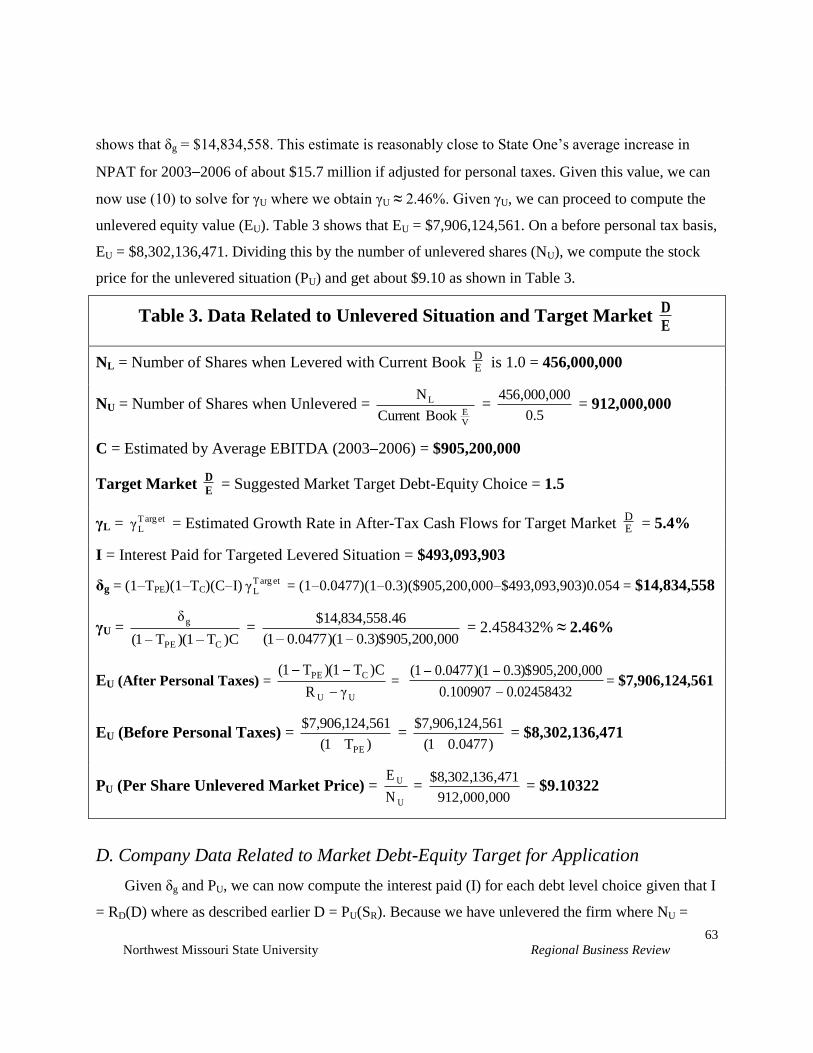
Firm Value And The Debt-Equity Choice · firms without long-term debt are a rarity as shown by...

Northwest Missouri State University Regional Business Review

50

Regional Business Review, Vol. 24, May 2005, pp.50-75

Firm Value And

The Debt-Equity Choice

Professor Rob Hull, School of Business, Washburn University

Abstract

Building on the no growth perpetuity framework first developed by Modigliani and Miller

(1963), this paper attempts to offer gain to leverage (GL) formulations useable by managers in

making debt-equity choices. These formulations focus on how changes in equity and debt

discount rates influence firm value. A real world application (using data suggested by

independent analysts) seeks to determine the gain to leverage for different debt-equity choices.

Using our formulation with constant growth, we offer results that can support the suggested

target debt-equity choice as the choice that maximizes firm value.

I. Introduction and Background

According to Compustat, since the beginning of the century there have been about 1,650 firms

per year that on average have reported no long-term debt (which includes capitalized lease

obligations). Gopalakrishnan (1994) indicates about 30 percent of such unlevered firms will issue

debt within a year and maintain it for a prolonged (if not permanent) period of time. However, larger

firms without long-term debt are a rarity as shown by Agrawal and Nagarajan (1990) who find only

104 such firms listed on major U.S. stock exchanges. This suggests that most managers, at least for

larger firms, behave as if value can be added by choosing some positive debt level when financing

their operating assets.

Theoreticians offer various formulas to support the managerial decision to issue debt. The

forerunner of this line of research is Modigliani and Miller (1963), referred to as MM. They derive a

gain to leverage (GL) formulation in the context of an unlevered firm issuing risk-free debt to replace

risky equity. For MM, GL is the corporate tax rate multiplied by debt value. The applicability of

MM’s GL formulation is limited as it implies that financial executives issue unrestricted amounts of

debt. Extensions of MM consider a variety of leverage-related wealth effects (most noteworthy, the


51

effects stemming from personal tax, flotation costs, bankruptcy, agency, and asymmetric information

considerations).

Empirical researchers offer differing opinions concerning the strength of leverage-related

effects. While early researchers (Warner, 1977; Miller, 1977) suggest such effects may be

unimportant (at least for larger firms), later investigators (Altman, 1984; Cutler and Summers 1988)

contend otherwise indicating such effects would be significant if quantified. Graham and Harvey

(2001) offer support for leverage-related effects but restrict this support by noting there is little

evidence that executives are concerned about some effects (namely, personal taxes, transactions

costs, asset substitution, free cash flows, and asymmetric information). Regardless of the significance

of leverage-related effects, some researchers (Graham and Harvey, 2001; Pinegar and Wilbrecht,

1989) indicate that firms may be more concerned with an amount of debt that gives flexibility for

future opportunities. Other researchers (Fischer, Heinkel, and Zechner, 1989; Kayhan and Titman,

2004) downplay the need for debt flexibility by offering evidence for the role performed by tax and

bankruptcy cost effects. Hull (1999) presents event study evidence consistent with leverage-related

effects determining an optimal debt level.

Given the presence of debt in the capital structure of most firms as well as the empirical

evidence concerning leverage-related effects, there is a need to offer usable equations that can

quantify these effects. This paper aims to fill this void by offering GL formulations that quantify

leverage-related wealth effects. This is done through perpetuity GL formulations that make explicit

how changes in equity and debt discount rates impact firm value. To the extent changes in such

discount rates can be accurately estimated along with values for other relevant variables (such as

growth and tax rates), the GL formulations given in this paper can be used to measure the dollar

impact of a proposed capital structure change. Consequently, it is possible for financial executives to

make a debt-equity choice that maximizes firm value.

The remainder of the paper is organized as follows. Section II reviews the traditional GL

perpetuity formulations. Section III derives GL formulations for an unlevered firm situation (although

not shown in this paper, similar but lengthier formulations could be offered for firms that are already

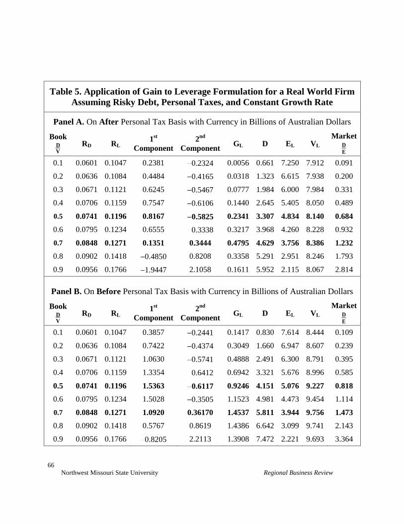
levered). Section IV gives computations for an application using real data. Section V reports the

application’s results for ten key variables for nine debt-equity choices. Section VI presents

limitations of the application and Section VII gives summary statements.


52

II. Traditional Perpetuity Gain to Leverage Formulations

This paper’s GL formulations are rooted in and developed within the no growth perpetuity

framework of MM (1963) and Miller (1977). This section reviews these GL formulations and their

extensions. It ends by indicating the need to incorporate discount rates in GL formulations.

A. The MM Gain to Leverage Formulation

MM analyze the valuation impact of a debt-for-equity transaction. The simplifying conditions

explicitly or implicitly used in their analysis include:

(i) two security types (an unlevered firm with risky equity that issues risk-free debt);

(ii) only corporate taxes (no personal taxes on income from either equity or debt);

(iii) level perpetuities (which can approximate any series of unequal cash flows);

(iv) no growth (depreciation each year equals investment to keep the same amount of capital);

(v) no imperfections (i.e., no leveraged-related effects such as flotation costs, bankruptcy costs,

agency effects, or asymmetric information effects); and,

(vi) equivalent return classes (the CAPM had not yet been developed).

Given these conditions, MM argue that GL is the exogenous corporate tax rate (TC) times the

value of perpetual risk-free debt (D) such that

GL = TCD. (1)

D is the chosen perpetual interest payment (I) divided by the exogenous cost of capital on risk-free

debt (RF). As D increases, MM posit that there is an increase in the rate at which risky equity is

discounted. However, no quantitative application is made of any net negative impact on firm value of

the increase in equity's discount rate. Similarly, no detailed valuation analysis is made of the GL

ramifications if debt is risky. However, if debt is risky, then we have

D = DR

I (2)

where RD > RF with RD now an increasing function of debt.

While there are other forms of financing that might affect the debt-equity choice, little attention

is given to these forms. For example, one form that might affect the choice is long-term lease

financing. However, because any such lease payment acts like debt by lowering the firm’s taxable

income and increasing its financial risk, it resembles debt and can be treated as part of D. This is true

for any off-balance-sheet items that behave like debt.


53

B. Extensions of the MM Formulation

Those extending the GL equation of MM (Baxter, 1967; Kraus and Litzenberger, 1973; Kim,

1978) assume risky debt. They argue that increasing debt levels are associated with increasing

bankruptcy costs such that an optimal debt level exists where the negative bankruptcy costs effect

offsets the positive tax shield effect. Increasing levels of debt can cause firm value to fall for reasons

other than bankruptcy costs. For example, Jensen and Meckling (1976) examine a wider range of

leverage-related costs that they call agency costs. Regardless of corporate tax shield and bankruptcy

considerations, net agency effects can impact GL. For example, increasing debt can initially cause net

gains owing to the reduction in owner-manager monitoring costs, but can eventually lead to net

losses due to the escalation in costs caused by restrictive debt covenants.

Drawing from the work of Farrar and Selwyn (1967), Miller (1977) assumes personal taxes and

extends (1) such that

GL = [1 α]D (3)

where α = )T1(

)T1)(T1(

PD

CPE with TPE and TPD the personal tax rates applicable to income from equity

and debt, and D now equalsD

PD

R

I)T1(. For Miller, costs related to the increase in debt (in particular,

bankruptcy costs) are inconsequential so that the effect of personal taxes alone offset the effect of

corporate taxes. For example, Miller argues that α ≈ 1, and thus GL ≈ zero (e.g., GL = [1 α]D ≈ [1

1]D ≈ 0). Regardless, as [1 α] in (3) takes on values smaller than TC, then GL in (3) becomes less

than GL in (1). Even if [1 α] = TC , GL in (3) is less than GL in (1) if TPD > 0 since D in (3) is

adjusted for personal taxes and now equals D

PD

R

I)T1( instead of just

DR

I.

Even if Miller is correct, signaling theory (Leland and Pyle, 1977; Ross, 1977; Myers and

Majluf, 1984) suggest that an increase in a firm’s debt-to-equity ratio can lead to an increase in firm

value. For example, Myers and Majluf (1984) argue that if managers are better informed than outside

investors, firms are more likely to retire equity when it is undervalued. Thus, a debt-for-equity

transaction would signal positive news in the sense underpriced securities are being retired (in

addition to any other positive signal the firm conveys about it future cash flows covering larger


54

interest payments). Empirical research (Copeland and Lee, 1991; Hull and Michelson, 1999) offers

evidence consistent with debt-for-equity transactions signaling positive news (including the

conveyance of reduced risk as seen in lower betas and thus reduced required rates of return). In

conclusion, signaling theory suggests exchanging debt for equity can cause GL > 0 to hold even if

there are no other leverage-related effects.

Ensuing GL extensions of MM (DeAngelo and Masulis, 1980; Kim, 1982; Modigliani, 1982;

Ross, 1985) consider a variety of leverage-related costs and show that an optimal debt level exists

even when personal taxes are recognized. Leland and Toft (1996) extend the closed-form results of

Leland (1994) to a much richer class of possible debt structures permitting the study of the optimal

amount of maturity of debt. Leland (1998) attempts to provide quantitative guidance on the amount

and maturity of debt, the financial restructuring, and the optimal risk strategy. For the most part, the

GL extensions are characterized by the inability to make explicit how changes in equity and debt

discount rates impact firm value within a model that financial managers might find useable.

III. Formulations That Incorporate Discount Rates

In this section, practical GL formulations are derived for managers making their debt-equity

choices. These equations consider the impact of equity and debt discount rates for an unlevered firm

for three situations: (i) no personal taxes and no growth, (ii) personal taxes and no growth, and, (iii)

personal taxes and constant growth.

A. Gain to Leverage Formulation without Personal Taxes

A GL formulation that includes discount rates can be derived from the definition that GL is

levered firm value (VL) minus unlevered firm value (VU). We have

GL = VL VU (4)

where VU and VL are defined below and the general MM conditions described earlier hold.

VU is the same as unlevered equity value (EU). EU is the uncertain perpetual after-corporate tax

cash flow available to unlevered equity of (1 TC)C divided by the exogenous unlevered equity

discount rate (RU). We have

VU = EU =U

C

R

C)T(1 (5)

where C is the perpetual before-tax cash flow available to unlevered equity owners with RU > RD if


55

the firm should choose to issue debt. Note that C assumes all expenses are cash expenses so that

before-tax cash flow equals taxable income.

VL is levered equity value (EL) plus debt value (D). EL is the uncertain perpetual after-corporate

tax cash flow available to levered equity of (1 TC)(C I) divided by the endogenous levered equity

discount rate (RL). We have

EL =L

C

R

)IC)(T(1 (6)

where RL > RU with RL positively related to debt (e.g., the cash flow to equity owners has more

uncertainty as debt increases). Inserting (6) and (2) into the definition VL = EL + D gives

VL = L

C

R

)IC)(T(1+

DR

I (7)

where RD = RF only if debt is risk-free debt (as MM assume or as the CAPM suggests when a debt

beta is assumed to be zero, which is often the assumption). Regardless, the derivation of the below

GL formulation is unimpeded if RD is endogenously determined by the debt level choice such that RD

> RF holds.

The GL formulation for an unlevered firm issuing debt can now be derived. After substituting (7)

into (4) and noting VU = EU, Appendix A shows

GL =L

D

R

Rα1 D + 1

R

R

L

U EU (8)

where α = (1 TC).

The 1st component, L

D

R

Rα1 D, is always positive if D > 0 since

L

D

R

Rα < 1. If D = 0, then this

component is zero. The 2nd component, 1R

R

L

U EU, is always negative if D > 0 since EU > 0 and

L

U

R

R< 1. If D = 0, then RU = RL and the 2nd component (like the 1st component) will also be zero

when D = 0 holds. Thus, if D = 0 then (8) implies that GL = 0. But if D > 0 then (8) can be either

positive or negative depending on which component has the greatest absolute value.

One can note that the 1st component is similar to the traditional GL formulations except α is


56

multiplied by a value less than one (e.g., L

D

R

R < 1) causing the component to be more positive than

the traditional GL formulations. In looking at the 2nd component, we can see that GL can be viewed as

being related to how much the increase in debt negatively affects outstanding equity through the

percentage increase in its discount rate. This relationship is consistent with the intuitive notion that as

leverage increases risk (and thus the required rate of return) then the value of the firm should fall

accordingly.

B. Gain to Leverage Formulation with Personal Taxes and Constant Growth

When personal taxes are considered, we can show (in a fashion similar to that found in

Appendix A and later in Appendix B) that GL can still be expressed as (8) if definitions for α, VU, EL,

and D are modified to incorporate personal tax rates. For example, we still have

GL = L

D

R

Rα1 D + 1

R

R

L

U EU

for (8) only now we have: α =)T1(

)T1)(T1(

PD

CPE ; VU = EU =R

C)T)(1T-(1

U

CPE; D =

R

I)T(1

D

PD; and, EL

=L

CPE

R

)IC)(T)(1T(1. For the 1st component to still be positive (when D > 0) is now a bit more

complicated. This is because, for L

D

R

Rα< 1 to now hold, restrictions must be placed on TC, TPE, and

TPD (and these restrictions depend on values for RD and RL).

Just as the Miller (1977) GL formulation given in (3) reduces to the MM formulation given in (1)

if TPE = TPD, so this paper’s GL formulation given in (8) reduces to (1) if RU = RL = RD and TPE = TPD.

With definitions for α, VU, EL, and D modified to include personal tax rates, equation (8) reduces to

the Miller formulation given by (3) if RU = RL = RD. These reductions reflect the MM derivational

procedure that assumes equality of discount rates when denominations (discount rates) are ignored in

the factoring process.

Appendix B derives a GL equation when both personal taxes and constant growth is considered.

Constant growth implies a current dollar change in after-tax cash flows (δg), which we define as

δg = (1 TPE)(1 TC)(C I)( etargTLγ ) (9)


57

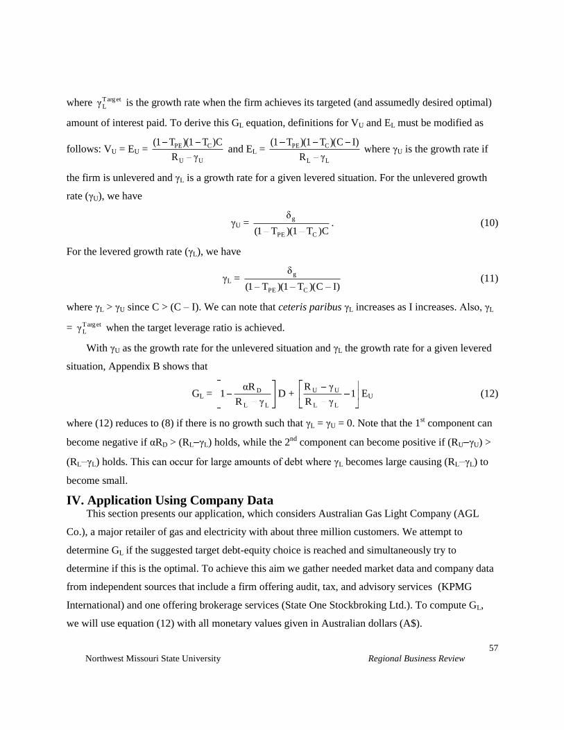
where etargTLγ is the growth rate when the firm achieves its targeted (and assumedly desired optimal)

amount of interest paid. To derive this GL equation, definitions for VU and EL must be modified as

follows: VU = EU = UU

CPE

γR

C)T)(1T(1 and EL =

LL

CPE

γR

)IC)(T)(1T(1 where γU is the growth rate if

the firm is unlevered and γL is a growth rate for a given levered situation. For the unlevered growth

rate (γU), we have

γU = C)T1)(T1(

δ

CPE

g. (10)

For the levered growth rate (γL), we have

γL = )IC)(T1)(T1(

δ

CPE

g (11)

where γL > γU since C > (C – I). We can note that ceteris paribus γL increases as I increases. Also, γL

= etargTLγ when the target leverage ratio is achieved.

With γU as the growth rate for the unlevered situation and γL the growth rate for a given levered

situation, Appendix B shows that

GL = LL

D

γR

Rα1 D + 1

γR

γR

LL

UU EU (12)

where (12) reduces to (8) if there is no growth such that γL = γU = 0. Note that the 1st component can

become negative if αRD > (RL γL) holds, while the 2nd component can become positive if (RU γU) >

(RL γL) holds. This can occur for large amounts of debt where γL becomes large causing (RL γL) to

become small.

IV. Application Using Company Data This section presents our application, which considers Australian Gas Light Company (AGL

Co.), a major retailer of gas and electricity with about three million customers. We attempt to

determine GL if the suggested target debt-equity choice is reached and simultaneously try to

determine if this is the optimal. To achieve this aim we gather needed market data and company data

from independent sources that include a firm offering audit, tax, and advisory services (KPMG

International) and one offering brokerage services (State One Stockbroking Ltd.). To compute GL,

we will use equation (12) with all monetary values given in Australian dollars (A$).


58

A. Market and Tax Rate Data for Application

From http://www.ipart.nsw.gov.au/papers/KPMG_February_04.pdf, we find a 48 page report on

AGL Co. where KPMG estimates values for variables that affect AGL Co.’s valuation. In Table 1,

we give KPMG’s suggestions (as of February 2004) for market and tax rate data.

Table 1. Market and Tax Rate Data

RR = Real Rate = 3.42%

RINF = Inflation Rate = 2.17%

RF = Risk-Free Rate = RR + RINF + (RR)(RINF) = 3.42% + 2.17% + (3.42%)(2.17%) = 5.6642%

MPREM = Market Premium = (RM – RF) = 6.00%

TC = Corporate Tax Rate = 30.00%

λ = Imputation Tax Credit = 40.00%

TE = Effective Tax Rate = TC(1–λ) = 30%(1 – 0.4) = 18.00%

TE = Effective Tax Rate = )]λ1(T[1

T1

C

C = )]4.01(3.0[1

3.01 = 0.14634 or 14.634%

Average TE = (18.00% + 14.634%) = 16.317% ≈ 16.32%

Average (1 – TE) = 1 – 0.16317 = 0.83683 ≈ 83.68%

TPE = Personal Tax Rate on Equity Income = 4.77%

TPD = Personal Tax Rate on Debt Income = 20.34%

α = )T1(

)T1)(T1(

PD

CPE = )2034.01(

)3.01)(0477.01(= 0.83682 ≈ 83.68% ≈ Average (1 – TE)

(1 – α) = (1 – 0.83682) = 0.16318 ≈ 16.32% ≈ Average TE

KPMG gives no estimates for personal tax rates so we turn to another approach that uses

knowledge of imputation credits (λ). Under the Australian imputation tax system, domestic equity

investors receive a taxation credit for dividends paid out of after-tax firm returns. In essence, an

imputation tax system offsets the corporate tax advantage of debt in a manner analogous to when

equity owners have a lower tax rate than debt owners (TPE < TPD). KPMG suggests that λ = 0.4 and

that TC (for equity owners) is effectively reduced to a lower rate (TE). As seen in Table 1, using the

average of the computations given by KPMG, we get Average TE = 16.317% ≈ 16.32%. Using this


59

value to estimate the personal tax rates, we proceed by noting that α = (1 TE) ≈ 1 0.1632 ≈ 0.8368

or about 83.68%. This value for α can be equated with a number of values for TPE and TPD (when TC

= 30%) including the two we use in our application: TPE = 4.77% and TPD = 20.34%. As seen in

Table 1, for these two values, α ≈ 83.68%.

We should point out that after personal tax values for EU, D, EL and VL when TC = 30%, TPE =

4.77%, and TPD = 20.34% will differ from those when TC (given by TE) = 16.32%, TPE = 0 and TPD =

0. However, if we look at before personal tax values for GL, the reductions in after personal tax

values for EU, D, EL and VL caused by using TPE = 4.77% and TPD = 20.34% will be overcome from

the standpoint of getting values before lowered by paying personal taxes.

Table 2. Beta and Cost of Capital Data

Current Book ED =

000,000,153,3$

000,500,241,3$≈ 1.0 implies

VD = 0.5 and

VE = 0.5

DPREM = Debt Premium = βD(RM – RF) = βD(MPREM) = 1.75%

βD = Debt Beta = DPREM / MPREM = 1.75% / 6% = 0.291667

RD = Cost of Debt = RF + βDMPREM = 5.66421% + 0.291667(6%) = 7.41421% ≈ 7.41%

βL = Levered Equity Beta = 1.05

RL = Cost of Levered Equity = RF + βLMPREM = 5.6642% + 1.05(6%) = 11.9642% ≈ 11.96%

βU = Unlevered Equity Beta = [ (1 )( )]

1 [(1 )( )]

DL D C E

DC E

T

T =

1.05 [0.291667(1 0.3)(1.0)]

1 [(1 0.3)(1.0)] = 0.737745

RU = Cost of Unlevered Equity = RF + βUMPREM = 5.664214% + 0.737745(6%) = 10.0907%

B. Beta and Cost of Capital Data for Application

As seen in Table 2, the annual report for AGL Co.’s fiscal year ending June 2004 indicates its

current book ED

ratio ≈ 1.0 where D is total liabilities and E is shareholders’ equity. The values

suggested by KPMG for betas and costs of capital are assumed to correspond with this book debt-

equity choice of 1.0. To get AGL Co.’s cost of debt, we begin by noting that KPMG estimates a debt

margin of 1.75%, which absent other costs suggests a debt premium (DPREM) of 1.75%. As seen in

Table 2, this premium implies the debt beta (βD) = 0.2917. Using the CAPM, we get the cost of debt


60

(RD) ≈ 7.41%, which is the midpoint of KPMG’s range estimated at 7.21% to 7.61%. KPMG

suggests AGL Co.’s levered beta (βL) = 1.05. Using the CAPM, this value for βL implies its cost of

levered equity (RL) ≈ 11.96%.

. KPMG indicates, regardless of any formula chosen, BD should not be assumed zero when

computing the unlevered beta (βU). Given TC = 30%, the current book leverage ratios ( ED

= 1.0, VD =

0.5, and VE = 0.5), βL = 1.05, and βD = 0.29, Table 2 uses the formula given by Hamada (1972) to get

βU = 0.7377. Using the CAPM, this value for βU implies the cost of unlevered equity (RU) =

10.0907%.

Given the data in Table 2, we can try to estimate betas (and thus RD’s and RL’s) for various debt

level choices. For simplicity, we consider only nine VD

choices with each choice given in book

values (before market adjustments caused by a positive GL are made). We determine each choice

based on the number of shares retired. This is accomplished by noting AGL Co. has outstanding

levered shares (NL) of 456,000,000. Given NL and current book VE

= 0.5, we can estimate the number

of shares if the firm was unlevered (NU). As will be seen in Table 3, we have

NU = Book Current

N

VE

L = 5.0

000,000,456 = 912,000,000.

From this NU value, we can get the number of shares retired (SR) for each debt level choice. For

example, if VE

= 0.9, then VD

= 0.1 and AGL Co. would retire SR = ( VD

)(NU) = 0.1(912,000,000) =

91,200,000 shares. Similarly, we can compute SR for any debt level choice. For each choice faced by

an unlevered firm, the value of the debt issued (D) should ceteris paribus equal the dollar amount of

the retired shares where D = PU(SR) with PU the unlevered share price (which can be viewed as the

current market price minus any gains to leverage).

Based on our nine VD

choices from 0.1 to 0.9, we can attempt to construct nine corresponding

βD’s and βL’s from which we can compute RD’s and RL’s needed in our GL formulation. We begin by

estimating debt betas (βD’s). The estimation process is based on the observation that we have two

βD’s endpoints and a βD interior point. This is seen below.

For the 1st endpoint when VD = 0, we have βD = 0.


61

For the interior point when VD = 0.5, we have (from Table 2) βD = 0.2977.

For the 2nd endpoint when VD 1.0, we have βD βU = 0.7377.

Concerning the latter, we see that as a firm approaches an all-debt situation with all shares retired, it

must legally revert to an all-equity firm and the unlevered beta of 0.7377.

Using linear interpolation, we can estimate the βD’s for each book VD

choice from 0.1 to 0.9. We

can then use the CAPM to get each corresponding RD. We show the βD and RD values below.

Debt Betas & Costs of Debt for Book VD Choices from 0.1 to 0.9

0.1 0.2 0.3 0.4 0.5 0.6 0.7 0.8 0.9

βD 0.058 0.117 0.175 0.233 0.292 0.381 0.470 0.559 0.649

RD 6.01% 6.36% 6.71% 7.06% 7.41% 7.94% 8.48% 9.02% 9.56%

For βL’s, we have only one endpoint ( VD

= 0, βL = βU = 0.7377) and an interior point ( VD

= 0.5,

βL = 1.05), ruling out linear interpolation for all choices. Given βD’s and βU, we use Hamada (1972)

to estimate βL’s. However, estimates using this equation break down as we approach high debt levels

because the βL’s values generate the same small linear increase of 0.06245 for each successive book

VD

choice from 0.6 to 0.9. Because of its linear relationship that treats the latter incremental increases

in debt as equally risky, the Hamada equation clearly cannot accommodate any expected rapidly

increasing levels of financial risk as we reach extreme debt levels. Thus, for the last two choices, our

application uses βL’s of 1.42 and 2.00 instead of the linear values given by Hamada (1.23735 and

1.29980). βL’s of 1.42 and 2.00 represent an increase of about 20% and 40% over respective previous

βL’s, and are deemed a more acceptable attempt to capture the increasing levels of financial risk. The

decision to start increasing βL’s for the 8th and 9th debt level choice is consistent with the target

leverage ratio that is set for AGL Co. so as to avoid undue financial distress. It remains for future

research to explore if there can be found a formula for βL supporting the observation that firms do not

strive for extreme high levels of debt.

Below we display the βL’s and RL’s for the book VD

choices from 0.1 to 0.9 with the CAPM used

to compute RL’s.


62

Equity Betas & Costs of Equity for Book VD Choices from 0.1 to 0.9

0.1 0.2 0.3 0.4 0.5 0.6 0.7 0.8 0.9

βL 0.800 0.863 0.925 0.988 1.050 1.112 1.174 1.420 2.000

RL 10.47% 10.84% 11.21% 11.59% 11.96% 12.34% 12.71% 14.18% 17.66%

C. Data Related to Unlevered Situation and Market Target ED for Application

Given RL’s and RD’s for the nine debt-equity choices, we can get EU and EL by estimating values

for C, etargTLγ , PU, I, δg, and γU. We estimate the perpetual before-tax cash flow for unlevered equity

owners (i.e., we estimate C) from http://www.stateone.com.au/documents/research/agl.pdf, which

gives earnings before interest and taxes plus depreciation / amortization (EBITDA). For the years

from 2003 to 2006, the average EBITDA suggests that C = $905.2 million.

Next, we estimate the growth rate for an unlevered situation (γU). We begin by trying to

determine current dollar change in after-tax cash flows (δg) as given by (9) where δg =

(1 TPE)(1 TC)(C I)(γL) with γL defined as the levered growth rate when the firm achieves its

targeted amount of interest paid (e.g., γL = etargTLγ ). Noting that KPMG indicates that AGL Co.’s

target ED

ratio is 1.5 (which we take as the market ratio since KPMG uses the word ―market‖ when

describing the weights from this choice), we proceed to estimate the future growth rate for after-tax

cash flows given this target. We settle on etargTLγ = 5.4% .This estimate is consistent with data

suggested by State One and AGL Co. reports. For example, State One (December 2004) estimates

that the net profit after tax will change from $320.8 million for June 2003 to $370.4 million for June

2006. The implied growth rate in after-tax cash flows = γL = 18.320$

4.376$ 3

1

≈ 5.5%. A similar value is

found (γL ≈ 5.3%) if we take the average of the growth in dividends from June 2003 to June 2006 and

the standard formula where the growth rate equals retention rate times required rate of return.

To proceed with estimating δg, we next need to compute the interest paid (I) when γL = 5.4%. As will

be seen later in Table 5, it is for the 7th debt level choice when 70% of unlevered shares are retired

(book choice of VD

= 0.7) that we attain the market target ED

≈ 1.5 ( ED

≈ 2.33 from a share

standpoint). As we will show later, I = $493,093,903 for this 7th choice. Using equation (9), Table 3


63

shows that δg = $14,834,558. This estimate is reasonably close to State One’s average increase in

NPAT for 2003 2006 of about $15.7 million if adjusted for personal taxes. Given this value, we can

now use (10) to solve for γU where we obtain γU ≈ 2.46%. Given γU, we can proceed to compute the

unlevered equity value (EU). Table 3 shows that EU = $7,906,124,561. On a before personal tax basis,

EU = $8,302,136,471. Dividing this by the number of unlevered shares (NU), we compute the stock

price for the unlevered situation (PU) and get about $9.10 as shown in Table 3.

Table 3. Data Related to Unlevered Situation and Target Market E

D

NL = Number of Shares when Levered with Current Book ED

is 1.0 = 456,000,000

NU = Number of Shares when Unlevered = Book Current

N

VE

L = 5.0

000,000,456 = 912,000,000

C = Estimated by Average EBITDA (2003 2006) = $905,200,000

Target Market E

D = Suggested Market Target Debt-Equity Choice = 1.5

γL = etargTLγ = Estimated Growth Rate in After-Tax Cash Flows for Target Market E

D = 5.4%

I = Interest Paid for Targeted Levered Situation = $493,093,903

δg = (1 TPE)(1 TC)(C I) etargTLγ = (1 0.0477)(1 0.3)($905,200,000 $493,093,903)0.054 = $14,834,558

γU = C)T1)(T1(

δ

CPE

g =

000,200,905)$3.01)(0477.01(

46.558,834,14$ = 2.458432% ≈ 2.46%

EU (After Personal Taxes) = UU

CPE

γR

C)T)(1T(1 =

02458432.0100907.0

000,200,905)$3.0)(10477.0(1= $7,906,124,561

EU (Before Personal Taxes) = )T1(

561,124,906,7$

PE

= )0477.01(

561,124,906,7$ = $8,302,136,471

PU (Per Share Unlevered Market Price) = U

U

N

E =

000,000,912

471,136,302,8$ = $9.10322

D. Company Data Related to Market Debt-Equity Target for Application

Given δg and PU, we can now compute the interest paid (I) for each debt level choice given that I

= RD(D) where as described earlier D = PU(SR). Because we have unlevered the firm where NU =


64

912,000,000 and PU = $9.10322, we can view each debt level choice for our unlevered firm as D =

PU(SR) where SR is the number of shares being retired for that choice. Since SR = ( VD

)(NU), we have

D = PU( VD

)(NU). Inserting this expression for D into I = RD(D), we get I = RD(PU)( VD

)(NU). Although

the details are omitted, we can note that from this relationship, we solve for the earlier value for I =

$493,093,903 for the 7th debt level choice. This is because we can create a quadratic equation where I

is a function of TC, TPE, C, RD, RU, etargTLγ , NU, and SR, all of which are known.

Table 4. Company Data Related to Market Debt-Equity Target

(Values for Market Debt-Equity Choice = 1.5 which is Book Debt-Firm Value Choice = 0.7)

R = Unlevered Shares Exchanged = VD

NU = 0.7(912,000,000) = 638,400,000 shares

BookVD = Book Value Leverage Choice Given by Shares Retired =

UN

R =

000,000,912

000,400,638 = 0.7

D (Before Personal Tax) = Amount of EU Retired = PU(R) = $9.10322(638,400,000) = $5,811,495,529

I (Interest Paid) = RDD = 0.084848($5,811,495,529) = $493,093,903

EL =LL

CPE

γR

)IC)(T)(1T(1=

054.012713626.0

)903,093,493$000,200,905)($3.0)(10477.0(1= $3,756,195,004

D = R

I)T(1

D

PD =

08484802.0

903)$493,093,2034.0(1 = $4,629,437,339

Target Market E

D (On Before Personal Tax Basis) =

)0477.01( / 004,195,756,3$

)2034.01( / 339,437,629,4$ = 1.473 ≈ 1.5

GL using (12) = LL

D

γR

Rα1 D + 1

γR

γR

LL

UUEU = $135,068,376 + $344,439,406 = $479,507,782

1st Component =

LL

D

γR

Rα1 D =

054.012713626.0

)08484802.0)(836819.0(1 $4,629,437,339 = $135,068,376

2nd

Component = 1γR

γR

LL

UUEU = 1

054.012713626.0

024584323.010090685.0$7,906,124,561 = $344,439,406

VL = EL + D = $3,756,195,004 + $4,629,437,339 = $8,385,632,343

GL using (4) = VL – VU = $8,385,632,343 – $7,906,124,561 = $479,507,782


65

With our firm unlevered, we can now illustrate the computation I for any debt level choice from this

unlevered condition, which is the condition assumed to apply when using (12). Consider the 1st

choice where book VD

= 0.1 and RD = 6.0142%. We have: I = RD (PU)( VD

)(NU) =

0.06014214($9.10322)(0.1)(912,000,000) = $49,930,825. Similarly, we can compute I for all

choices. For the 7th choice, we can verify that I = $493,093,903 for book VD

= 0.7. We have: I = RD

(PU)( VD

)(NU) = 0.084848($9.10322)(0.7)(912,000,000) = $493,093,903. As seen in Table 4, this

interest payment corresponds very closely to the target market debt-equity choice of 1.5.

After computing I for each debt level choice, we can use (11) and compute γL for each choice.

For example, for the 1st debt level choice, we get

γL = )IC)(T1)(T1(

δ

CPE

g =

)825,930,49$000,200,905)($3.01)(0477.01(

8.46$14,834,55 = 2.601956%.

We obtain the following γL values for the nine debt level choices: 2.602%, 2.783%, 3.016%, 3.318%,

3.725%, 4.370%, 5.400%, 7.270%, and 11.637%. The growth rates begin increasing much more

rapidly as I C causing the 1st and 2nd components of (12) to eventually flip signs.

Given γL for each debt level choice, we can use (12) or (4) to get GL for each corresponding debt

level choice. We do this in Table 4 for the 7th debt level choice and show that GL = $479,507,782 on

an after personal tax basis. The table also shows that this choice corresponds with a target market ED

≈ 1.5 when computed on a before personal tax basis.

V. Results for All Nine Debt Level Choices for the Application

This section summarizes the results of our application in table form. We give gain to leverage

(GL) results for the unlevered application for AGL Co. for all nine debt level choices. The application

assumes the previously mentioned data including the betas needed to compute the costs of capital.

Conditions of our application are formally stated below so as to include values for key variables.

(a) debt is risky with RD > RF = 5.6642%, and RD is positively related to debt.

(b) tax rates are relevant with TPE = 4.77%, TPD = 20.34%, and TC = 30%;

(c) uncertain perpetual before-tax cash flows to unlevered equity: C = $905,200,000;

(d) constant growth rate when target market ED

approximated: etargTLγ = 5.4% with current dollar change

(δg) = $14,834,558; and,

(e) an unlevered firm with risky equity faces a finite set of perpetual debt-for-equity choices with RL > RU

= 10.0907%.


66

Table 5. Application of Gain to Leverage Formulation for a Real World Firm

Assuming Risky Debt, Personal Taxes, and Constant Growth Rate

Panel A. On After Personal Tax Basis with Currency in Billions of Australian Dollars

Book

VD

RD RL 1

st

Component

2nd

Component GL D EL VL

Market

E

D

0.1 0.0601 0.1047 0.2381 0.2324 0.0056 0.661 7.250 7.912 0.091

0.2 0.0636 0.1084 0.4484 0.4165 0.0318 1.323 6.615 7.938 0.200

0.3 0.0671 0.1121 0.6245 0.5467 0.0777 1.984 6.000 7.984 0.331

0.4 0.0706 0.1159 0.7547 0.6106 0.1440 2.645 5.405 8.050 0.489

0.5 0.0741 0.1196 0.8167 0.5825 0.2341 3.307 4.834 8.140 0.684

0.6 0.0795 0.1234 0.6555 0.3338 0.3217 3.968 4.260 8.228 0.932

0.7 0.0848 0.1271 0.1351 0.3444 0.4795 4.629 3.756 8.386 1.232

0.8 0.0902 0.1418 0.4850 0.8208 0.3358 5.291 2.951 8.246 1.793

0.9 0.0956 0.1766 1.9447 2.1058 0.1611 5.952 2.115 8.067 2.814

Panel B. On Before Personal Tax Basis with Currency in Billions of Australian Dollars

Book

VD

RD RL 1

st

Component

2nd

Component GL D EL VL

Market

E

D

0.1 0.0601 0.1047 0.3857 0.2441 0.1417 0.830 7.614 8.444 0.109

0.2 0.0636 0.1084 0.7422 0.4374 0.3049 1.660 6.947 8.607 0.239

0.3 0.0671 0.1121 1.0630 0.5741 0.4888 2.491 6.300 8.791 0.395

0.4 0.0706 0.1159 1.3354 0.6412 0.6942 3.321 5.676 8.996 0.585

0.5 0.0741 0.1196 1.5363 0.6117 0.9246 4.151 5.076 9.227 0.818

0.6 0.0795 0.1234 1.5028 0.3505 1.1523 4.981 4.473 9.454 1.114

0.7 0.0848 0.1271 1.0920 0.36170 1.4537 5.811 3.944 9.756 1.473

0.8 0.0902 0.1418 0.5767 0.8619 1.4386 6.642 3.099 9.741 2.143

0.9 0.0956 0.1766 0.8205 2.2113 1.3908 7.472 2.221 9.693 3.364


67

Table 5 reports results for ten key variables when financial managers face nine debt choices

given in the nine rows. Panel A reports results (where applicable) on an after personal tax basis while

Panel B focuses on before personal tax results. As discussed previously, the before personal tax

results are important because they can minimize inaccuracies in the after personal tax results that

might result if personal tax rates are closer in value than what we use.

Each panel has two bold-faced rows. The 1st bold-faced row is for the current situation where

book VD

= 0.5, while the 2nd bold-faced row is for book VD

= 0.7, which is where GL is maximized for

both panels. As seen in the last column of Panel B, it is also the row which is nearest the market

target ED

of 1.5. For this row, we get GL = $1.4537 billion on a before personal tax basis (which is

what the market sees). For this row, dividing EL by the number of outstanding shares (NL), we get a

share price ≈ $14.42. For example, with VD

= 0.7 (or VE = 0.3), we have NL = V

E (NU) =

0.3(912,000,000) = 273,600,000 shares giving the market share price as:

PBefore Personal Tax = L

L

N

E =

shares 000,600,273

023,340,944,3$ = $14.4164 per share.

This is less than the average market price at the time of this writing, which has averaged $13.83 for

January 2005. Thus, $14.42 can be considered a prediction of the future price (absent effects beyond

those stemming from the increased debt) if the market target is achieved.

The prediction for the stock price at the time we begin estimating values for our variables

(February 2004) can be computed for the 1st bold-faced row where NL = 456,000,000 shares. We

have:

PBefore Personal Tax = L

L

N

E =

shares 000,000,456

792,687,075,5$ = $11.1309 per share.

This price is consistent with both the average price of $11.06 for AGL Co. for February 2004 and

also for the average price of $11.29 for the year of the 2003 annual report (7/1/03 to 6/30/04).

GL on a before personal tax basis in Panel B is greater than the after personal tax basis in Panel

A given that personal taxes are subtracted from GL in Panel A. The difference is sizeable as seen

when comparing the maximum GL value of $0.4795 billion in Panel A with the corresponding

maximum value of $1.4537 billion in Panel B. In looking at Panel B, we can also point out, that due


68

to the increase in equity that accrues from GL, the book ED

of 2.333 (from a share standpoint) is

reduced to a market ED

of 1.473. This is near the target of 1.5.

While the maximum GL is achieved in both panels with the 7th debt level choice, it does not

necessarily follow that both panels will agree. It may be even more likely that the after personal tax

GL can be achieved for a different debt level choice than the before personal GL. If decisions are

actually made on what is best for investors, the firm would arguably choose the debt level where GL

is maximized on an after personal tax basis. However, absent perfect knowledge about personal tax

rates and given our restriction to nine debt level choices (where this restriction tends to

underestimates the maximum GL and the optimal ED

), it appears that the firm’s maximum GL on a

before personal tax basis will occur within a ED

range of about 1.4 to 2.0. This range is consistent

with values reported by http://www.bizstats.com/currentratios.htm. For example, BizStats give a

debt-to-equity ratio of 1.79 for U.S.A. gas production and distribution utilities.

Although both GL components experience change in signs as more debt is added, this is not

necessarily always the case. Absent a large value for δg that leads to large values for γL for high debt

levels, we would expect the 1st component to always be positive and the 2nd component to always be

negative.

VI. Limitations of Application

In this section, we call attention to four limitations facing our application. In general, such

limitations are found in all models that rely on accurate estimates of values for its variables.

First, personal tax rates were not directly known. This limitation was ameliorated through use of

an effective tax rate and analysis of before personal tax values.

Second, most firms are levered. Thus, to apply our GL formulation, we have to unlever our firm

in an attempt to estimate the number of shares outstanding (NU) if it had no debt. From here we

determine book debt-to-equity choices. Given these choices and the unlevered price (PU), we can

determine how much debt will be issued for each choice. The application depends on the accuracy of

estimating NU and PU and is limited if these estimates lack sufficient accuracy.

Third, we encountered a roadblock when computing betas. For example, we had to interpolate

from endpoints and a midpoint to get reasonable βD’s for each debt level choice. From there we


69

proceeded to get βU and then obtain βL’s for the nine debt level choices by using standard formulas.

However, unless adjusted upward, the βL computations for higher debt levels would suggest that

firms aim for extremely high leverage targets, which we do not find in the real world. This limitation

(in getting sufficient estimates for at least some betas) caused us to make intuitive ad hoc

assignments for levered equity betas at higher levels of debt. Future research needs to explore other

ways of estimating betas and costs of capital such as suggested by researchers who offer alternatives

methods (Fama and French, 1997; Lally, 2004).

Finally, the application had to estimate a current dollar level of growth (δg) based on a chosen

growth rate at the target debt-equity choice. Using Excel, we were able to solve for δg and the interest

paid (I) at the market target debt-equity choice based on values for other variables.

VII. Summary Statements

This paper derives GL formulations based on definitions for unlevered and levered firm values.

Such formulations include discount rates for unlevered equity, levered equity, and debt. The

inclusion of these rates makes it possible for GL values to eventually decrease with increasing debt

levels. Three GL formulations for an unlevered situation are offered to aid managers (when making

the debt-equity choice) and educators (when explaining the ramifications of the debt-equity choice).

The application using market data and company data for AGL Co. showed how managers can

use the GL formulation with personal taxes and constant growth to understand how the debt-equity

choice can influence firm value. While this paper’s model (like any model) relies on accurate

estimates of values for variables, the model’s optimal GL was able to conform to the recommended

market target ED

of 1.5 by assuming escalating values for levered equity’s beta at higher levels of

debt.

This study is important for several reasons. First, prior research offers formulations that are

difficult for practitioners in that they do not fully address the role of discount rates, and tend to be

unrealistic by including variables that are virtually immeasurable in themselves (e.g., direct and

indirect bankruptcy costs and agency costs). As such, financial managers are hard pressed to find

utility in their application. To the extent changes in discount rates are easier to estimate, this paper's

GL formulations offer more practical potential.

Second, the practical application in this paper suggests a wealth maximizing debt-equity choice


70

where the actual choice can depends on taxes and growth rates in addition to changes in discount

rates. The application produces results that re-enforce and strengthen general conclusions of prior

empirical and theoretical research in regard to the belief that increasing levels of debt can cause G L

to begin falling. The increase in G L, followed by a decrease, can be explained through the interaction

of many factors (such as taxes, bankruptcy costs, and agency effects) that together determine a firm’s

optimal debt-equity choice.

In conclusion, the GL formulations found in this paper reaffirm, synthesize, and extend prior GL

formulations, while opening up a fresh vista from which to view the debt-equity choice faced by

managers. This vista offers a practical vantage point in that capital structure decision-making can be

based on formulations that include variables heretofore not fully utilized.


71

Appendix A: GL for Unlevered Firm with No Personal Taxes

Proof of equation (8): For the situation of an unlevered firm when only corporate taxes are

considered, substituting (7) into (4) and noting VU = EU gives

GL = L

C

R

)IC)(T(1 +

DR

I EU.

Multiplying out the 1st component, noting

DR

I = D, and rearranging:

GL = D L

C

R

I)T(1 EU +

L

C

R

C)T(1.

Multiplying the 2nd

component by D

D

R

R gives

DL

DC

R

I

R

R)T(1 , which is

L

DC

R

R)T(1 D, and

factoring out D:

GL = L

DC

R

R)T1(1 D EU +

L

C

R

C)T(1.

Multiplying the last component by U

U

R

R gives

L

U

R

R

U

C

R

C)T(1, which is

L

U

R

REU, and factoring

out EU:

GL = L

DC

R

R)T1(1 D

L

U

R

R1 EU.

Setting α = (1 TC) and noting L

U

R

R1 EU = + 1

R

R

L

U EU gives

GL =L

D

R

Rα1 D + 1

R

R

L

U EU. (8)

Q.E.D.


72

Appendix B: GL for Unlevered Firm with Personal Taxes and Constant Growth

Proof of equation (12): Assume constant growth such that γL > γU > 0 and personal taxes such

that VU = EU = UU

CPE

γR

C)T)(1T(1 and EL =

LL

CPE

γR

)IC)(T)(1T(1. Substituting VL = EL + D =

LL

CPE

γR

)IC)(T)(1T(1 + D into (4) and noting VU = EU gives:

GL = LL

CPE

γR

)IC)(T)(1T(1 + D EU.

Multiplying out the 1st component and rearranging:

GL = D LL

CPE

γR

I)T)(1T(1 EU +

LL

CPE

γR

C)T)(1T(1.

Multiplying the 2nd

component by DPD

DPD

R)T(1

R)T(1 gives

D

PD

LL

D

PD

CPE

R

I)T1(

γR

R

)T1(

)T1)(T1(,

which is LL

D

PD

CPE

γR

R

)T1(

)T1)(T1(D, and factoring out D:

GL = LL

D

PD

CPE

γR

R

)T1(

)T1)(T1(1 D EU +

LL

CPE

γR

C)T)(1T(1.

Multiplying the last component by UU

UU

γR

γR = 1 gives

LL

UU

γR

γR

UU

CPE

γR

C)T)(1T(1, which is

LL

UU

γR

γREU, and factoring out EU:

GL = LL

D

PD

CPE

γR

R

)T1(

)T1)(T1(1 D

LL

UU

γR

γR1 EU.

Setting α = )T1(

)T1)(T1(

PD

CPE and noting LL

UU

γR

γR1 EU = + 1

γR

γR

LL

UU EU gives

GL = LL

D

γR

Rα1 D + 1

γR

γR

LL

UU EU. (12)

Q.E.D.


73

References Agrawal, Anup and Nandu Nagarajan, 1990, "Corporate Capital Structure, Agency Costs, and

Ownership Control: The Case of All-Equity Firms," Journal of Finance, 45 (3), 1325-1331.

Altman, Edward, 1984, "A Further Empirical Investigation of the Bankruptcy Cost Question,"

Journal of Finance, 39 (September), 1067-1087.

Baxter, Nevins, 1967, "Leverage Risk of Ruin and the Cost of Capital." Journal of Finance 22

(September), 395-403.

BizStats.com, [December 2004] report on Current Ratios and Other Balance Sheet Ratios. Retrieved

Dec. 7, 2004. http://www.bizstats.com/currentratios.htm

Copeland, T. and Won Lee, 1991, ―Exchange Offers and Stock Swaps—New Evidence,‖ Financial

Management 20 (Autumn): 34-48.

Cutler, David and Lawrence Summers, 1988, "The Costs of Conflict Resolution and Financial

Distress: Evidence from the Texaco-Pennzoil Litigation," Rand Journal of Economics, 19 (Summer), 157-

172.

DeAngelo, Harry and Ronald Masulis, 1980, "Optimal Capital Structure Under Corporate and

Personal Taxation," Journal of Financial Economics, 8 (March), 3-30.

Gopalakrishnan, V., 1994, "Accounting Choice Decisions and Unlevered Firms: Further Evidence on

Debt/Equity Hypothesis,‖ Journal of Financial and Strategic Decisions, 7 (Fall, Number 3), 33-47.

Fama, Eugene and Kenneth French, 1997, ―Industry Costs of Equity,‖ Journal of Financial

Economics, 43, 153-193.

Hamada, Robert, 1972, ―Effect of a Firm’s Capital Structure on the Systematic Risk of Common

Stocks,‖ Journal of Finance, 27 (May), 435-452.

Harvey, Campbell and John Graham, 2001, ―The Theory and Practice of Corporate Finance:

Evidence from the Field,‖ Journal of Financial Economics, 60 (May), 187-243.

Farrar, D. and L. Selwyn, 1967, "Taxes, Corporate Financial Policy, and Returns to Investors,"

National Tax Journal, 20, 444-454.

Fischer, Edwin O., Robert Heinkel and Josef Zechner, 1989, "Optimal Dynamic Capital Structure

Choice: Theory and Tests,‖ The Journal of Finance, 44, 19-40.

Hull, Robert, 1999, ―Leverage Ratios, Industry Norms, and Stock Price Reaction: An Empirical

Investigation of Stock-for-Debt Transactions, Financial Management, 28 (Summer, Number 2), 32-45.


74

Hull, Robert and Stuart E. Michelson, 1999, ―The Information Contents of Senior Offerings that

Reduce Junior Securities,‖ Quarterly Review of Economics and Finance, 39 (Fall, Number 3), 419-438.

Jensen, M. and W. Meckling, 1976, "Theory of the Firm: Managerial Behavior, Agency Costs and

Ownership Structure," Journal of Financial Economics, 3 (October), 305-360.

Kayhan, Ayla and Sheridan Titman, 2004, ―Firms’ Histories and Their Capital Structure,‖ NBER

Working Paper No. W10526.

Kim, E. Han, 1978, "A Mean-Variance Theory of Optimal Capital Structure and Corporate Debt

Capacity," Journal of Finance, 33 (March), 45-63.

Kim, E. Han, 1982, "Miller's Equilibrium, Shareholder Leverage Clienteles, and Optimal Capital

Structure," Journal of Finance, 37 (May), 301-320.

KPMG, [February 2004] report on AGL Gas Networks, Ltd. Retrieved Dec. 11, 2004.

http://www.ipart.nsw.gov.au/papers/KPMG_February_04.pdf.

Kraus, Alan and Robert Litzenberger, 1973, "A State-Preference Model of Optimal Capital

Structure," Journal of Finance, 28 (September), 911-922.

Lally, Martin, 2004, ―The Fama-French Model, Leverage, and the Modigliani-Miller Propositions,‖

The Journal of Financial Research, 27 (September), 341-349.

Leland, Hayne and David Pyle, 1977, ―Informational Asymmetries, Financial Structure, and

Financial Intermediation,‖ Journal of Finance, 32 (May), 371-388.

Leland, Hayne, 1994, "Corporate Debt Value, Bond Covenants, and Optimal Capital Structure,"

Journal of Finance, 49 (September), 1213-1252.

Leland, Hayne and Klaus Toft, 1996, ―Optimal Capital Structure, Endogenous Bankruptcy, and the

Term Structure of Credit Spreads,‖ Journal of Finance, 51 (July), 261-275.

Leland, Hayne, 1998, ―Agency Costs, Risk Management, and Capital Structure,‖ Journal of Finance,

53 (August), 1213-1243.

Miller, Merton, 1977, "Debt and Taxes," Journal of Finance, 32 (May), 261-275.

Modigliani, Franco and Merton Miller, 1963, "Corporate Income Taxes and Cost of Capital: A

Correction," American Economics Review, 48 (June), 433-443.

Modigliani, Franco, 1982, "Debt, Dividend Policy, Taxes, Inflation and Market Valuation," Journal

of Finance, 37, 255-273.


75

Myers, S. and N. Majluf, 1984, ―Corporate Financing and Investment Decisions when Firms Have

Information that Investors Do Not Have,‖ Journal of Financial Economics 13 (June): 187-221.

Pinegar, J. Michael, and Lisa Wilbrecht, 1989, "What Managers Think of Capital Structure Theory: A

Survey." Financial Management 18 (Winter), 82-91.

Ross, Stephen, 1977, ―The Determination of Financial Structure: The Incentive-Signaling

Approach,‖ Bell Journal of Economics, 8 (Spring): 23-40.

Ross, Stephen, 1985, "Debt and Taxes and Uncertainty," Journal of Finance, 40 (Spring), 637-658.

State One Stockbroking Ltd., [December 2004] report of The Australian Gas Light Company.

Retrieved Dec. 17, 2004. http://www.stateone.com.au/documents/research/agl.pdf

Warner, J., 1977, "Bankruptcy Costs: Some Evidence," Journal of Finance, 26 (May), 337-348.

Date post:	14-Apr-2018
Category:	Documents
Upload:	trinhthuy
View:	215 times
Download:	2 times

Firm Value And The Debt-Equity Choice · firms without long-term debt are a rarity as shown by...

Documents