First Order Driving Simulator - EECS at UC Berkeley · First Order Driving Simulator ... like to...

First Order Driving Simulator

Wesley Hsieh

Electrical Engineering and Computer SciencesUniversity of California at Berkeley

Technical Report No. UCB/EECS-2017-102http://www2.eecs.berkeley.edu/Pubs/TechRpts/2017/EECS-2017-102.html

May 12, 2017

Copyright © 2017, by the author(s).All rights reserved.

Permission to make digital or hard copies of all or part of this work forpersonal or classroom use is granted without fee provided that copies arenot made or distributed for profit or commercial advantage and that copiesbear this notice and the full citation on the first page. To copy otherwise, torepublish, to post on servers or to redistribute to lists, requires priorspecific permission.


by

Wesley Hsieh

A thesis submitted in partial satisfaction of therequirements for the degree of

Master of Science

in

Electrical Engineering and Computer Science

in the

Graduate Division

of the

University of California, Berkeley

Committee in charge:

Professor Ken Goldberg, ChairProfessor Trevor Darrell

Spring 2017

The dissertation of Wesley Hsieh, titled First Order Driving Simulator, is approved:

Chair Date

Date

Date



Copyright 2017by

Wesley Hsieh

1

Abstract


by

Wesley Hsieh

Master of Science in Electrical Engineering and Computer Science


Professor Ken Goldberg, Chair

Autonomous driving is a complex task that features high variability in everyday driving condi-tions due to the presence of vehicles and different road conditions. Many data-centric learningmodels require exposure to a high number of data points collected in various driving conditionsto be robust to this variability. We present the First Order Driving Simulator (FODS), an open-source lightweight driving simulator designed for data collection and benchmarking performancefor autonomous driving experiments, with a focus on customizability and speed. The car model iscontrolled using steering, acceleration, and braking as inputs. The car features the choice betweenkinematic and dynamic bicycle models with slip and friction, as a first-order approximation to thedynamics of a real car. Users can customize features including the track, vehicle placement, andother initial conditions of the environment, as well as environment interface features such as thestate space (images, positions and poses of cars) and action space (discrete or continuous controls,limits). We benchmark our performance against other simulators of varying degrees of complex-ity, and show that our simulator matches or outperforms their speeds of data collection. We alsofeature parallelization with Ray [36], a distributed execution framework aimed at making it easyto parallelize existing codebases, which allows for significant speed increases in data collection.Finally, we also perform experiments analyzing the performance of various imitation learning andreinforcement learning algorithms on our simulator environment.

i

Contents

Contents i

List of Figures iii

List of Tables iv

1 Introduction 2

2 Related Work 52.1 Benchmarking . . . . . . . . . . . . . . . . . . . . . . . . . . . . . . . . . . . . . 52.2 Driving Simulators . . . . . . . . . . . . . . . . . . . . . . . . . . . . . . . . . . 5

3 Dynamics 103.1 Point Model . . . . . . . . . . . . . . . . . . . . . . . . . . . . . . . . . . . . . . 103.2 Kinematic Bicycle Model . . . . . . . . . . . . . . . . . . . . . . . . . . . . . . . 113.3 Dynamic Bicycle Model . . . . . . . . . . . . . . . . . . . . . . . . . . . . . . . 11

4 System Features 134.1 System Architecture . . . . . . . . . . . . . . . . . . . . . . . . . . . . . . . . . . 134.2 Customization . . . . . . . . . . . . . . . . . . . . . . . . . . . . . . . . . . . . . 134.3 Parallelization . . . . . . . . . . . . . . . . . . . . . . . . . . . . . . . . . . . . . 15

5 Benchmarking 175.1 Simulator Comparison . . . . . . . . . . . . . . . . . . . . . . . . . . . . . . . . 175.2 Results . . . . . . . . . . . . . . . . . . . . . . . . . . . . . . . . . . . . . . . . . 175.3 Parallelization . . . . . . . . . . . . . . . . . . . . . . . . . . . . . . . . . . . . . 185.4 Results . . . . . . . . . . . . . . . . . . . . . . . . . . . . . . . . . . . . . . . . . 18

6 Experiments 206.1 Configuration . . . . . . . . . . . . . . . . . . . . . . . . . . . . . . . . . . . . . 206.2 Evaluation . . . . . . . . . . . . . . . . . . . . . . . . . . . . . . . . . . . . . . . 206.3 Imitation Learning . . . . . . . . . . . . . . . . . . . . . . . . . . . . . . . . . . . 206.4 Reinforcement Learning . . . . . . . . . . . . . . . . . . . . . . . . . . . . . . . 22

ii

7 Discussion and Future Work 247.1 Discussion . . . . . . . . . . . . . . . . . . . . . . . . . . . . . . . . . . . . . . . 247.2 Future Work . . . . . . . . . . . . . . . . . . . . . . . . . . . . . . . . . . . . . . 24

Bibliography 26

iii

List of Figures

2.1 TORCS . . . . . . . . . . . . . . . . . . . . . . . . . . . . . . . . . . . . . . . . . . 62.2 GTA V . . . . . . . . . . . . . . . . . . . . . . . . . . . . . . . . . . . . . . . . . . . 72.3 Udacity’s Driving Simulator . . . . . . . . . . . . . . . . . . . . . . . . . . . . . . . 72.4 OpenAI Gym: CarRacing-v0 Environment . . . . . . . . . . . . . . . . . . . . . . . . 82.5 Driving Interactions: Simulator . . . . . . . . . . . . . . . . . . . . . . . . . . . . . . 9

4.1 Examples of different terrain, with different coefficients of friction. . . . . . . . . . . . 144.2 Examples of different track configurations. . . . . . . . . . . . . . . . . . . . . . . . . 154.3 Architecture of Ray processing pipeline. . . . . . . . . . . . . . . . . . . . . . . . . . 16

5.1 Simulator performance benchmarking results. Left image is benchmarking with ren-dering. Right image is benchmarking with rendering disabled. . . . . . . . . . . . . . 18

5.2 Simulator parallelization benchmarking results. Left image is benchmarking with ren-dering. Right image is benchmarking with rendering disabled. . . . . . . . . . . . . . 19

6.1 Environment used for Experiments . . . . . . . . . . . . . . . . . . . . . . . . . . . . 216.2 Examples of states considered as crashes in the experiment. Left image illustrates an

example of colliding with a car. Right image illustrates an example of running off themain road. . . . . . . . . . . . . . . . . . . . . . . . . . . . . . . . . . . . . . . . . . 22

6.3 Performance of Imitation Learning Algorithms . . . . . . . . . . . . . . . . . . . . . 226.4 Performance of Reinforcement Learning Algorithms . . . . . . . . . . . . . . . . . . 23

iv

List of Tables

3.1 Road Friction Coefficients . . . . . . . . . . . . . . . . . . . . . . . . . . . . . . . . 12

5.1 Steps (x1000) per Minute, Rendering . . . . . . . . . . . . . . . . . . . . . . . . . . . 175.2 Steps (x1000) per Minute, No Rendering . . . . . . . . . . . . . . . . . . . . . . . . . 18

v

Acknowledgments

I would first like to thank my research advisor Professor Ken Goldberg for the opportunity to workin the AUTOLAB. Working in an academic research environment has made the past few yearsof my undergraduate and graduate career an incredible experience. Professor Ken Goldberg hasprovided many great ideas and insights on both the direction and presentation of the work I havedone throughout my stay here.

I especially thank my mentor Michael Laskey for supporting me throughout my research ex-perience here, from whom I have learned so much from collaborating with him over the past fewyears. He provided an endless stream of advice on everything from research questions to futurecareers. I am incredibly grateful for the opportunity to work with him, and his advice has been amajor key to the work I have done here.

I would also like to thank the other members of the AUTOLAB for contributing to a greatresearch environment. I am incredibly humbled by the amount of work that is put into all of thevarious projects there, as well as the availability and willingness of its members to help each other.

I also thank Professor Trevor Darrell for his help on my master’s thesis committee, as well aseverything I have learned from his computer vision class last year.

Finally, I would like to thank my family for their support throughout the last four years of myundergraduate and graduate career at the University of California, Berkeley.

1

Abstract


by

Wesley Hsieh

Master of Science in Electrical Engineering and Computer Science


Professor Ken Goldberg, Chair

Autonomous driving is a complex task that features high variability in everyday driving condi-tions due to the presence of vehicles and different road conditions. Many data-centric learningmodels require exposure to a high number of data points collected in various driving conditionsto be robust to this variability. We present the First Order Driving Simulator (FODS), an open-source lightweight driving simulator designed for data collection and benchmarking performancefor autonomous driving experiments, with a focus on customizability and speed. The car model iscontrolled using steering, acceleration, and braking as inputs. The car features the choice betweenkinematic and dynamic bicycle models with slip and friction, as a first-order approximation to thedynamics of a real car. Users can customize features including the track, vehicle placement, andother initial conditions of the environment, as well as environment interface features such as thestate space (images, positions and poses of cars) and action space (discrete or continuous controls,limits). We benchmark our performance against other simulators of varying degrees of complex-ity, and show that our simulator matches or outperforms their speeds of data collection. We alsofeature parallelization with Ray [36], a distributed execution framework aimed at making it easyto parallelize existing codebases, which allows for significant speed increases in data collection.Finally, we also perform experiments analyzing the performance of various imitation learning andreinforcement learning algorithms on our simulator environment.

2

Chapter 1

Introduction

Autonomous driving has increasingly become a popular area of research especially in the pastfew years. Many major companies including Google, Tesla, NVIDIA, and Uber have alreadydedicated teams of researchers into development of self driving cars. Smaller companies andstartups built around autonomous driving and related products have also sprung up recently.

Autonomous driving requires precision in perception and robustness to varying conditions ofthe environment. Due to the high-speed nature of driving, where critical decisions are often re-quired within seconds, controllers for autonomous cars must also be able to plan and execute inreal-time. The environment itself is partially observed; sensor observations of the environment aresubject to noise and occlusion from other objects in the environment [30]. In addition to learninghow to navigate the desired path safely, controllers face a large degree of variability in everydaydriving conditions due to the presence of pedestrians, vehicles, and other occupants of the road[48], making it necessary to re-plan based on changes in the environment for safe trajectory plan-ning and execution. Additionally, safety is an especially important consideration of designing aself-driving car controller due to the large costs of a collision with another vehicle or object onthe road. Driving tasks also have a large time horizon, making frequent planning and re-planningextremely important to handle changes in the observed environment.

There have been many data-centric methods that have been proposed to train controllers forautonomous driving. All of these data-driven methods aim to acquire enough data and experienceto become robust to various changes in the environment that could occur during day-to-day driving.Imitation learning is a class of methods that involves training an autonomous agent to imitate asupervisor that is known to be proficient at the task at hand. In the case of autonomous driving,this agent is often a human in the real world or a classical control model that has access to thedynamics of the simulator environment. Examples of imitation learning methods applied to drivingenvironments include DAgger [42], SHIV [29], SafeDAgger [54], and Dart [28]. Reinforcementlearning methods have also been proposed and applied to driving environments; reinforcementlearning is a class of methods that involves learning from experience, where an agent’s actions aregiven feedback indirectly through a reward signal. The agent aims to balance exploration of newpolicies with exploitation of the currently known best policy. Examples of reinforcement learningmethods applied to driving environments include as Q-Learning [49], Vanilla Policy Gradient [50],

CHAPTER 1. INTRODUCTION 3

Trust Region Policy Optimization [45], Deep Deterministic Policy Gradient [31], and A3C [34].Because of the many safety and robustness requirements for autonomous driving, policies must

be able to re-plan quickly and adapt to various environments. Training a data-driven model requiresa large number of data samples to be robust to the environment due to the high dimensionality ofimage observations and high variance in the state space [9].

Collecting training data in the real world often features the assistance of human operators forlegal requirements and to ensure safety and quality of feedback [4], making data collection costly.

Training in simulation presents an avenue for safely collecting data without the large conse-quences of making a mistake, which is especially useful for training in the early stages of a modelwhere it is the most prone to crashing. Simulation also allows faster learning of safe driving be-haviors in the presence of other vehicles, which can be fine-tuned to adapt to real-world situations[16].

There exist many simulators that are currently being used in autonomous driving experiments.Simulators are used to determine the effectiveness of a new method specifically for autonomousdriving and control. Driving simulators have also been used as a general benchmarking environ-ment to evaluate the effectiveness of a new general-purpose algorithms. Many of these experimentsrequire large quantities of training data to perform, making data collection an expensive operation.TORCS, an open-source racing simulator, has been used in many research experiments [34, 10, 37,33, 32]. Similarly, Grand Theft Auto has also been used as a data source for experiments relatedto the driving domain [17, 41]. Research groups and labs have also independently developed theirown driving simulators of varying complexities for their own experiments.

We present a lightweight driving simulator designed primarily for autonomous driving exper-iments, with a focus on customizability and speed of integration with existing learning pipelines.We design the simulator as a first-order approximation of a driving environment to be used as abenchmarking tool to quickly evaluate the effectiveness of a new method for autonomous driving,especially with consideration to the safety and data efficiency of the output policy. To simplify thestate space of the environment, we feature a 2D birds-eye view of the simulator centered around thecar, with simple graphics for performance. The car features the choice between point, kinematic,and dynamic bicycle models with slip and friction, as a first-order approximation to car dynamics.Its input controls include steering, acceleration, and braking, and can be input from an externalprogram or manually through a keyboard or Xbox controller. To facilitate ease of integration withexternal modules, the simulator implements the OpenAI Gym interface [8], a popular environmentinterface for learning problems.

Using the configuration module, many features of the simulator itself can be tweaked to fit thedesired task. On startup, the environment reads from this configuration file to set up its featuresincluding the track, car placement as well as environment features such as state space (images,positions and poses of cars) and action space (discrete or continuous, limits).

We also feature integration with Ray [36], a distributed execution framework aimed at makingit easy to parallelize existing codebases, including data collection for machine learning and rein-forcement learning applications. Experiments using this framework can significantly improve therate of data collection, which is often a bottleneck for learning experiments. Using a parallelization

CHAPTER 1. INTRODUCTION 4

framework like Ray is extremely important for reducing the costs of data collection especially fordata-intensive learning methods.

The goal of this simulator is to be able to quickly configure the environment to fit the desireddriving task, then quickly integrate with an existing learning model to start gathering data fortraining. We perform experiments benchmarking performance against other driving simulators.We also provide example code for integration with imitation learning and reinforcement learningalgorithms.

5

Chapter 2

Related Work

2.1 BenchmarkingOur work is related to data-centric end-to-end systems developed for autonomous driving.

ALVINN [39] was one of the first systems that leveraged neural networks to train a policy tomap from images to controls for driving; a similar approach was performed by Chen et al. using amore convolutional neural network model [13]. Xu et al. created an end-to-end system for learn-ing vehicle motion models from video datasets [52]. Bojarski et al. used supervised learning totrain end-to-end convolutional neural networks for driving in the real world [6], as well as provideexplanations and insight into what the system learns [7].

Our work is also related to vision benchmarks and tasks that are necessary for autonomousdriving. There exist benchmarks in the real world evaluate the ability of an autonomous drivingsystem to perceive important features of the surrounding environment. Dubbelman et al. createda dataset to benchmark stereo based motion estimation [15]. Geiger et al. created a dataset tobenchmark various perception tasks including stereo, optical flow, visual odometry, and 3-D objectdetection [19]. Fritsch et al. created a dataset to benchmark road area and lane detection in urbanareas [18].

Driving simulators have also been used to provide synthetic data for various tasks. Richter etal. created a synthetic dataset generated from Grand Theft Auto V to supplement real-world datafor training semantic segmentation systems [41]. TORCS [51], an open-source driving simulator,has been used to learn mid-level cues for autonomous driving that generalized to real images [12],and to benchmark imitation learning [10, 54], reinforcement learning [33], and genetic algorithms[37].

2.2 Driving SimulatorsThere are many existing simulators with varying degrees of complexity and different target

audiences. We compare to other simulators used for autonomous driving projects. All of these

CHAPTER 2. RELATED WORK 6

Figure 2.1: TORCS

feature similar control schemes, with steering, acceleration, and braking as the primary controlinputs to the car.

TORCS [51] is an open-source 3-D racing car simulator that allows implementation of con-trollers to race against computer opponents. The project is more complex than FODS and includesdynamics such as gears, fuel, damage, wheel velocities as well as other vehicles. Direct communi-cation with the game is possible with Java and C++, while there exists third-party Python interfaces[53] for communicating with the game through a client-server interface. There also exists a third-party Python library that also implements the Gym interface for ease of integration with externallearning pipelines. The viewpoint of the simulator is from the driver’s point of view. In comparisonto FODS, this simulator is more complex and features more customizability.

DeepGTAV [43] is an interface for communicating with an instance of Grand Theft Auto, apopular 3-D open-world sandbox game with a driving component. The game itself is proprietary,and requires purchase of a license to use. It communicates with the game through a client-serverinterface in Python, which transmits messages in JSON format. The simulator is in 3-D and theviewpoint is from behind the car. The environment includes realistic graphics and can include othercars. In comparison to FODS, this simulator is proprietary and more complex, and the environmentitself is designed for gaming purposes rather than for driving experiments.

Udacity features an open-source 3-D driving simulator rendered in Unity for their online courseon using deep learning to train an autonomous driving agent. The viewpoint for collecting data isfrom behind the car, while labeled images are generated from a first-person drivers perspective ofthe road. The project features two built-in tracks, as well as a custom track creation module. Incomparison to FODS, this simulator has less customizability, more complex graphics, and does notfeature other cars.

OpenAI Gym [8] features many built-in environments for evaluation of learning algorithms.


Figure 2.2: GTA V

Figure 2.3: Udacity’s Driving Simulator

Their driving environment is an open-source 2-D driving simulator implemented with Box2D [11].The state space is a top-down view of the environment, with the camera centered around the car.Slip and friction dynamics are implemented, and skid marks are rendered when the car slips. Incomparison with FODS, this simulator has less customizability and does not feature other cars onthe track.

Many research groups and labs have also independently developed their own driving simulatorsof varying complexities for their own experiments. Sadigh et al. created their own 2-D drivingsimulator as an environment for evaluating inverse reinforcement learning algorithms with a focuson interactions between different vehicles [44]. The viewpoint is a 2-D birds-eye view centeredaround the car and its surrounding environment. The dynamics model is specified symbolically


Figure 2.4: OpenAI Gym: CarRacing-v0 Environment

through Theano [5], which facilitates usage of classical control and other algorithms that requireknowledge of the dynamics.


Figure 2.5: Driving Interactions: Simulator

10

Chapter 3

Dynamics

There are many existing car dynamics models with differing degrees of complexity. We optedto use relatively simpler dynamics for the car to facilitate performance and simplicity while main-taining a first order approximation of a car. The car features the choice between point, kinematic,and dynamic bicycle models with slip and friction, as a first order approximation. Both models usesteering and acceleration and braking as input controls. The models are discretized using SciPy’s[24] ordinary differential equation integrator and is sampled at td = 100 ms. For simplicity andsimulator performance reasons, we opt not to use complete full vehicle dynamics models [2, 35,40].

3.1 Point ModelThe point model is the most simple dynamics model available for the simulator. The continuous

differential equations that describe the point bicycle models are as follows.

x = vcos(δ f ) (3.1)

y = vsin(δ f ) (3.2)

ψ = δ f (3.3)

v = a (3.4)

x and y are the coordinates of the center of mass in an inertial frame (X ,Y ). ψ is the inertialheading and v is the speed of the vehicle. a is the acceleration of the center of mass in the samedirection as the velocity. The control inputs are the front and rear steering angles δ f , δr, and a.Since in most vehicles the rear wheels cannot be steered, we assume δr = 0.

CHAPTER 3. DYNAMICS 11

3.2 Kinematic Bicycle ModelThe inertial position coordinates and heading angle in the kinematic bicycle model are defined

in the same manner as those in the point model. The continuous differential equations that describethe kinematic bicycle models are as follows [40, 27].

x = vcos(ψ +β ) (3.5)

y = vsin(ψ +β ) (3.6)

ψ =vlr

sin(β ) (3.7)

v = a (3.8)

β = tan−1(lr

l f + lrtan(δ f )) (3.9)

l f and lr represent the distance from the center of the mass of the vehicle to the front and rearaxles, respectively. β is the angle of the current velocity of the center of mass with respect to thelongitudinal axis of the car.

3.3 Dynamic Bicycle ModelThe inertial position coordinates and heading angle in the dynamic bicycle model are defined

in the same manner as those in the kinematic bicycle model. The continuous differential equationsthat describe the kinematic bicycle models are as follows.

x = ψ y+ax (3.10)

y =−ψ x+2m(Fc, f cosδ f +Fc,r) (3.11)

ψ =2Iz(l f Fc, f − lrFc,r) (3.12)

X = xcosψ− ysinψ (3.13)

Y = xsinψ + ycosψ (3.14)

x and y denote the longitudinal and lateral speeds in the body frame, respectively and ψ denotesthe yaw rate. m and Iz denote the vehicles mass and yaw inertia, respectively. Fc, f and Fc,r denotethe lateral tire forces at the front and rear wheels, respectively, in coordinate frames aligned withthe wheels.

For the linear tire model, Fc,i is defined as

Fc,i =−Cαiαi (3.15)

where i ∈ { f ,r},αi is the tire slip angle and Cαi is the tire cornering stiffness.

CHAPTER 3. DYNAMICS 12

Table 3.1: Road Friction Coefficients

Road Type µ

Dry 0.9Wet 0.6Snow 0.2Ice 0.05

We estimate the cornering stiffness as follows [47].

c f = µ ·m · lrl f + lr

·a f

δ f −a fv + r

(3.16)

This estimate is restricted to δ f −a fv + r 6= 0. Under the assumption of the linearized single

track model equations, this term is identical to α f . We therefore use the following estimate.

c f = µ ·m · lrl f + lr

(3.17)

We use the value of Iz ≈ 2500, which is a typical value for a smaller car [22].We also list the different coefficients of friction based on the road type [20].

13

Chapter 4

System Features

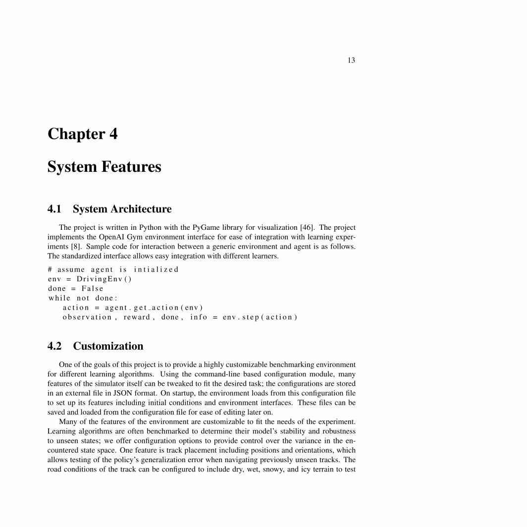
4.1 System ArchitectureThe project is written in Python with the PyGame library for visualization [46]. The project

implements the OpenAI Gym environment interface for ease of integration with learning exper-iments [8]. Sample code for interaction between a generic environment and agent is as follows.The standardized interface allows easy integration with different learners.

# assume a g e n t i s i n t i a l i z e denv = Dr iv ingEnv ( )done = F a l s ew h i l e n o t done :

a c t i o n = a g e n t . g e t a c t i o n ( env )o b s e r v a t i o n , reward , done , i n f o = env . s t e p ( a c t i o n )

4.2 CustomizationOne of the goals of this project is to provide a highly customizable benchmarking environment

for different learning algorithms. Using the command-line based configuration module, manyfeatures of the simulator itself can be tweaked to fit the desired task; the configurations are storedin an external file in JSON format. On startup, the environment loads from this configuration fileto set up its features including initial conditions and environment interfaces. These files can besaved and loaded from the configuration file for ease of editing later on.

Many of the features of the environment are customizable to fit the needs of the experiment.Learning algorithms are often benchmarked to determine their model’s stability and robustnessto unseen states; we offer configuration options to provide control over the variance in the en-countered state space. One feature is track placement including positions and orientations, whichallows testing of the policy’s generalization error when navigating previously unseen tracks. Theroad conditions of the track can be configured to include dry, wet, snowy, and icy terrain to test

CHAPTER 4. SYSTEM FEATURES 14

Figure 4.1: Examples of different terrain, with different coefficients of friction.

robustness to different vehicle handlings; similarly, the dynamics model of the main car can bechanged between the point, kinematic, and dynamic bicycle models to offer control over the ve-hicle’s handling. The number of computer-controlled cars, as well as their positions, velocities,orientations, and color can be changed to test the robustness of the policy to avoiding cars at vary-ing parts of the map. We also feature control over the randomization of car properties, includingpositions withing specified bounding boxes, distances between car placements, and starting angles,which allows for control over the large variance in the initial state distribution.

Additionally, many properties of the simulator itself can be customized to fit the needs of theexperimental pipeline and system. The simulator can be configured to set the rendering screen sizeas well as enabling or disabling rendering, which allows for significant performance increases forapplications that do not require image data. Similarly, we can configure the output state space,including rendered RGB color images, or positions, velocities, and orientations of cars. The sizeof the output image can also be downsampled to be smaller than the original rendered image usingOpenCV [23]. These options allow the state space to match the data formats needed by the model,as well as allow for performance increases for experiments without rendering. We also featurecustomization of the action space, including choice of discrete or continuous controls. The controllimits of the action space can also be modified, as well as the step size and size of the actionspace in the discrete case. Steering or acceleration and braking controls can also be disabled orenabled. These features allow control over the action space for the needs of the experiment. Thetime horizon of the environment can also be set, after which the environment automatically returnsTrue for its ”done” output when taking a step, to indicate that the environment should be reset;this allows for performing experiments with varying time lengths. Finally, the sampling rate forlogging of the states and actions encountered can be set, as well as its respective output location.


Figure 4.2: Examples of different track configurations.

Adding FeaturesAdditional configuration features can be easily added by modifying the configuration module

to add an additional entry and prompt into the existing list of features. Afterwards, the corre-sponding entry will appear to the environment on startup when it loads the configuration file. Theenvironment then can handle the entry as desired.

Advanced CustomizationAdditional features that are more complex and intrinsic to the environment, such as custom

reward functions, additional car dynamics models, or terrain models, can be implemented by cre-ation of custom classes that inherit from the corresponding environment, car, or terrain class, andoverwriting the corresponding functions. Under the hood, most objects that the environment inter-acts with has its own corresponding ”step” function for updates, which can be modified to handlemost changes.

4.3 ParallelizationWe feature integration with Ray [36], a distributed execution framework aimed at making it

easy to parallelize existing codebases. including data collection for machine learning and rein-forcement learning applications. Experiments using this framework can significantly improve therate of data collection, which is often a bottleneck for learning experiments. We provide an exam-ple of integration of Ray with imitation learning experiments, where we iteratively parallelize ourdata collection over multiple CPUs each with their own individual instance of the simulator, poolour simulated trajectories and rewards from the workers, then update our model with the data andtrain using a GPU.


Figure 4.3: Architecture of Ray processing pipeline.

17

Chapter 5

Benchmarking

5.1 Simulator ComparisonWe benchmark our performance against other simulators of varying degrees of complexity,

and show that our simulator matches or outperforms their speeds of data collection. All trials areperformed on a 12-processor Intel Core i7 CPU. We benchmark by measuring the amount of timethe simulator takes to reach 1000 steps over n = 10 trials. We also attempt to disable rendering andreport the corresponding times; this option has not been found to be possible especially for morecomplex simulators that couple rendering with the environment update.

5.2 ResultsWe find that the First Order Driving Simulator outperforms the other simulators that we bench-

mark against. We significantly outperform the 3-D simulators with over three times the speed ofthe next best simulator, as expected due to their higher detail and complexity in rendering. We alsooutperform the 2-D simulators with slightly under two times the speed of the next-best simulator.

Table 5.1: Steps (x1000) per Minute, Rendering

Simulator mean stdevFODS 3.48 0.0372Udacity 0.99 0.0623TORCS 0.29 0.0004Driving Interactions 0.56 0.0164OpenAI Gym (CarRacing-v0) 1.84 0.0526

CHAPTER 5. BENCHMARKING 18

Figure 5.1: Simulator performance benchmarking results. Left image is benchmarking with ren-dering. Right image is benchmarking with rendering disabled.

Table 5.2: Steps (x1000) per Minute, No Rendering

Simulator mean stdevFODS 58.3 6.321Udacity - -TORCS - -Driving Interactions - -OpenAI Gym (CarRacing-v0) 3.71 0.1017

5.3 ParallelizationWe also benchmark the effects of parallelization on the performance of FODS. We benchmark

by measuring the amount of time the simulator takes to reach 10000 steps over n = 10 trials, whilevarying the number of cores allotted to the simulator. We report results for rendering enabled anddisabled.

5.4 ResultsWe find that increasing the number of processors up to the maximum limit of 12 improves the

performance of the simulator, but there are diminishing returns due to additional overhead.

CHAPTER 5. BENCHMARKING 19

Figure 5.2: Simulator parallelization benchmarking results. Left image is benchmarking withrendering. Right image is benchmarking with rendering disabled.

20

Chapter 6

Experiments

We benchmark the performance of imitation learning and reinforcement learning methods onthis environment.

6.1 ConfigurationWe include the particular set of configurations used for these experiments. The agent’s car has

initial state variance uniform over [-30, 30] for starting angles. There are five other cars uniformlyscattered within a grid that spans up to 100 time steps forward in the road from the car’s currentlocation. The agent only has control over its steering and is forced to accelerate up to its maximumspeed at twice the speed of the other cars, forcing it to learn to steer around the other cars whileavoiding travelling off the road. The road is also narrow enough to make it impossible to turnaround.

6.2 EvaluationWe evaluate performance of a learning algorithm based on the average number of steps the

agent travels before the current trajectory is terminated. The current trajectory is marked as ”done”and terminated immediately when either the main car collides with another car or runs off the track,or if the maximum time horizon of 100 time steps is reached.

6.3 Imitation Learning

AlgorithmsOne set of experiments we perform is analyzing the performance of different imitation learning

algorithms on this environment. We evaluate DAgger [42], Dart [28], and ordinary supervisedlearning, as well as variants on these algorithms.

CHAPTER 6. EXPERIMENTS 21

Figure 6.1: Environment used for Experiments

ConfigurationsFor this set of experiments, the state space of the simulator is gray-scale 8-bit images of the

rendered image, in the set S = [0,255]300×300. Our neural net architecture features a convolutionallayer with 5 filters of dimension 7x7 and a fully connected hidden layer of dimension 60. Eachlayer is separated by ReLU non-linearities. The images are centered around the agent’s car. All ex-periments feature a cost-based search planner as a supervisor to provide demonstrations, which hasaccess to the lower dimensional internal state space of the simulator. The cost function is weightedto promote navigating around cars while keeping closer to the center of the road. The supervisoris able to achieve a reward of approximately 70 on average on this particular environment. Weprovide the results of these experiments, plotting average episode reward against the number ofdemonstrations provided by the supervisor.

ResultsOn this particular environment, we find that Dart-0.5 performs the best with an average score

of approximately 60. The other three imitation learning methods achieve lower scores around 40-50 by the end of the experiment. All of these imitation learning methods outperform ordinarysupervised learning, which achieves a score of approximately 20.


Figure 6.2: Examples of states considered as crashes in the experiment. Left image illustrates anexample of colliding with a car. Right image illustrates an example of running off the main road.

Figure 6.3: Performance of Imitation Learning Algorithms

6.4 Reinforcement Learning

AlgorithmsWe also perform another set of experiments evaluating the performance of different reinforce-

ment learning algorithms on this environment. We evaluate REINFORCE [50], Trust Region Pol-icy Optimization [45], Truncated Natural Policy Gradient [25, 3], and Reward Weighted Regres-sion [38, 26].


Figure 6.4: Performance of Reinforcement Learning Algorithms

ConfigurationsWe feature examples integrating the environment with Rllab [14], which features implemen-

tations of these as well as other reinforcement learning algorithms. For this set of experiments,to reduce the state space of the simulator, we provide the state space as the positions and posesof all of the cars, in the set R18. Each of these algorithms is run with a batch size of 40000 timesteps per update iteration, with a total of 500 iterations, and a step size of 0.01. Our neural netarchitecture features two fully connected hidden layers of size 64. Each layer is separated by tanhnon-linearities. Including overhead from parallelization, we collect around 200-250 time steps persecond per thread. We provide the results of these experiments, plotting average episode rewardagainst the number of update iterations taken by the reinforcement learning algorithms.

ResultsOn this particular environment, we find that Truncated Natural Policy Gradient (TNPG) and

Trust Region Policy Optimization (TRPO) perform the best with a score of approximately 35.Vanilla Policy Gradient (VPG) achieves a score around 32. Reward Weighted Regression (ERWR)achieves a score of around 30. All of these algorithms plateau and achieve their best performancearound 250 iterations.

24

Chapter 7

Discussion and Future Work

7.1 DiscussionWe present a lightweight simulator designed for autonomous driving experiments, with a focus

on customizability and speed of integration with existing learning pipelines.The state space is a2D birds-eye view of the simulator centered around the car, with simple graphics for performance.The car features the choice between kinematic and dynamic bicycle models with slip and friction.Its input controls include steering, acceleration, and braking, and can be input from an externalprogram or manually through a keyboard or Xbox controller.

To facilitate ease of integration with external modules, the simulator implements the OpenAIGym interface [8], a popular environment interface for learning problems. We also feature paral-lelization with Ray [36], a distributed execution framework aimed at making it easy to parallelizeexisting codebases, which allows for significant speed increases in data collection. We benchmarkour performance against other simulators of varying degrees of complexity, and show that oursimulator matches or outperforms their speeds of data collection.

7.2 Future WorkWhile the core functionality of the project has been implemented, there are multiple additional

features we wish to implement in the future to improve usability and performance.

GUIOne important feature is to create a graphical user interface for the configuration module, as

opposed to the current command-line interface. This will greatly improve the speed and usabil-ity of configuring the environment, especially for features that are more intuitively representedgraphically such as track placement.

CHAPTER 7. DISCUSSION AND FUTURE WORK 25

Box2DWe also wish to investigate porting the core of the system to Box2D [11], a two-dimensional

physics simulator for games that offers a Python interface [21]. Box2D is a more complete gameengine than PyGame due to better supported rendering features as well as direct native support forhandling physics simulations. We may offer a choice between the different backends dependingon comparisons of performance.

Symbolic Dynamics ModelsAnother possible feature is to allow specification of dynamics models symbolically in Tensor-

flow [1] or Theano [5]. Currently, the dynamics models for most simulators including this one areopaque and require inspection of the source code to extract. By specifying the models symboli-cally, the dynamics models become more readily usable for traditional motion planning approachesthat require knowledge of the dynamics model. This allows for easier comparisons between an-alytically planning models and data-driven machine learning approaches. Additionally, this willallow for easier imports of custom dynamics models, rather than directly implementing a sub-classof the car model and overwriting the corresponding functions.

Use CasesFrom a usability perspective, we also wish to improve the documentation of use cases of the

simulator. We hope to provide more examples of configurations for different simulator setups.We also hope to include more examples of scripts for running different imitation learning or rein-forcement learning algorithms, as well as integration with classical control algorithms that requiresymbolic specification of dynamics models.

26

Bibliography

[1] Martın Abadi et al. “Tensorflow: Large-scale machine learning on heterogeneous distributedsystems”. In: arXiv preprint arXiv:1603.04467 (2016).

[2] R Wade Allen et al. A low cost PC based driving simulator for prototyping and hardware-in-the-loop applications. Tech. rep. SAE Technical Paper, 1998.

[3] J Andrew Bagnell and Jeff Schneider. “Covariant policy search”. In: IJCAI. 2003.

[4] Sven A Beiker. “Legal aspects of autonomous driving”. In: Santa Clara L. Rev. 52 (2012),p. 1145.

[5] James Bergstra et al. “Theano: Deep learning on gpus with python”. In: NIPS 2011, BigLearn-ing Workshop, Granada, Spain. Vol. 3. Citeseer. 2011.

[6] Mariusz Bojarski et al. “End to end learning for self-driving cars”. In: arXiv preprint arXiv:1604.07316(2016).

[7] Mariusz Bojarski et al. “Explaining How a Deep Neural Network Trained with End-to-EndLearning Steers a Car”. In: arXiv preprint arXiv:1704.07911 (2017).

[8] Greg Brockman et al. “OpenAI gym”. In: arXiv preprint arXiv:1606.01540 (2016).

[9] Mark Campbell et al. “Autonomous driving in urban environments: approaches, lessons andchallenges”. In: Philosophical Transactions of the Royal Society of London A: Mathemati-cal, Physical and Engineering Sciences 368.1928 (2010), pp. 4649–4672.

[10] Luigi Cardamone, Daniele Loiacono, and Pier Luca Lanzi. “Learning drivers for TORCSthrough imitation using supervised methods”. In: Computational Intelligence and Games,2009. CIG 2009. IEEE Symposium on. IEEE. 2009, pp. 148–155.

[11] Erin Catto. Box2D. https://github.com/erincatto/Box2D. 2007.

[12] Chenyi Chen et al. “Deepdriving: Learning affordance for direct perception in autonomousdriving”. In: Proceedings of the IEEE International Conference on Computer Vision. 2015,pp. 2722–2730.

[13] Chenyi Chen et al. “Learning Affordance for Direct Perception in Autonomous Driving”.In: ().

[14] Yan Duan et al. “Benchmarking deep reinforcement learning for continuous control”. In:Proceedings of the 33rd International Conference on Machine Learning (ICML). 2016.

BIBLIOGRAPHY 27

[15] Gijs Dubbelman and Frans CA Groen. “Bias reduction for stereo based motion estimationwith applications to large scale visual odometry”. In: Computer Vision and Pattern Recog-nition, 2009. CVPR 2009. IEEE Conference on. IEEE. 2009, pp. 2222–2229.

[16] Azim Eskandarian. Handbook of intelligent vehicles. Springer London, 2012.

[17] Artur Filipowicz, Jeremiah Liu, and Alain Kornhauser. Learning to Recognize Distance toStop Signs Using the Virtual World of Grand Theft Auto 5. Tech. rep. 2017.

[18] Jannik Fritsch, Tobias Kuhnl, and Andreas Geiger. “A new performance measure and eval-uation benchmark for road detection algorithms”. In: Intelligent Transportation Systems-(ITSC), 2013 16th International IEEE Conference on. IEEE. 2013, pp. 1693–1700.

[19] Andreas Geiger, Philip Lenz, and Raquel Urtasun. “Are we ready for autonomous driving?the kitti vision benchmark suite”. In: Computer Vision and Pattern Recognition (CVPR),2012 IEEE Conference on. IEEE. 2012, pp. 3354–3361.

[20] Raymond Ghandour et al. “Tire/road friction coefficient estimation applied to road safety”.In: Control & Automation (MED), 2010 18th Mediterranean Conference on. IEEE. 2010,pp. 1485–1490.

[21] Gustavo Goretkin. pybox2d. https://github.com/pybox2d/pybox2d. 2011.

[22] Petr Hejtmanek et al. “Measuring the Yaw Moment of Inertia of a Vehicle”. In: Journal ofMiddle European Construction and Design of Cars 11.1 (2013), pp. 16–22.

[23] Itseez. Open Source Computer Vision Library. https://github.com/itseez/opencv. 2015.

[24] Eric Jones, Travis Oliphant, Pearu Peterson, et al. SciPy: Open source scientific tools forPython. [Online; accessed 2017]. 2001–. URL: http://www.scipy.org/.

[25] Sham M Kakade. “A natural policy gradient”. In: Advances in neural information processingsystems. 2002, pp. 1531–1538.

[26] Jens Kober and Jan R Peters. “Policy search for motor primitives in robotics”. In: Advancesin neural information processing systems. 2009, pp. 849–856.

[27] Jason Kong et al. “Kinematic and dynamic vehicle models for autonomous driving controldesign”. In: Intelligent Vehicles Symposium (IV), 2015 IEEE. IEEE. 2015, pp. 1094–1099.

[28] Michael Laskey et al. “Iterative Noise Injection for Scalable Imitation Learning”. In: arXivpreprint arXiv:1703.09327 (2017).

[29] Michael Laskey et al. “Shiv: Reducing supervisor burden in dagger using support vectors forefficient learning from demonstrations in high dimensional state spaces”. In: Robotics andAutomation (ICRA), 2016 IEEE International Conference on. IEEE. 2016, pp. 462–469.

[30] Jesse Levinson et al. “Towards fully autonomous driving: Systems and algorithms”. In: In-telligent Vehicles Symposium (IV), 2011 IEEE. IEEE. 2011, pp. 163–168.

[31] Timothy P Lillicrap et al. “Continuous control with deep reinforcement learning”. In: arXivpreprint arXiv:1509.02971 (2015).

BIBLIOGRAPHY 28

[32] Guan-Horng Liu, Sai Prabhakar, and Avinash Siravuru. “Deep-RL using Overcomplete StateRepresentation”. In: ().

[33] Daniele Loiacono et al. “Learning to overtake in torcs using simple reinforcement learning”.In: Evolutionary Computation (CEC), 2010 IEEE Congress on. IEEE. 2010, pp. 1–8.

[34] Volodymyr Mnih et al. “Asynchronous methods for deep reinforcement learning”. In: Inter-national Conference on Machine Learning. 2016, pp. 1928–1937.

[35] Russell Lee Mueller. “Full vehicle dynamics model of a formula SAE racecar using ADAMS/-Car”. PhD thesis. Texas A&M University, 2005.

[36] Robert Nishihara et al. Ray. https://rise.cs.berkeley.edu/projects/ray.2017.

[37] Diego Perez, Gustavo Recio, and Yago Saez. “Evolving a fuzzy controller for a car racingcompetition”. In: Computational Intelligence and Games, 2009. CIG 2009. IEEE Sympo-sium on. IEEE. 2009, pp. 263–270.

[38] Jan Peters and Stefan Schaal. “Reinforcement learning by reward-weighted regression foroperational space control”. In: Proceedings of the 24th international conference on Machinelearning. ACM. 2007, pp. 745–750.

[39] Dean A Pomerleau. ALVINN, an autonomous land vehicle in a neural network. Tech. rep.Carnegie Mellon University, Computer Science Department, 1989.

[40] Rajesh Rajamani. Vehicle dynamics and control. Springer Science & Business Media, 2011.

[41] Stephan R Richter et al. “Playing for data: Ground truth from computer games”. In: Euro-pean Conference on Computer Vision. Springer. 2016, pp. 102–118.

[42] Stephane Ross, Geoffrey J Gordon, and Drew Bagnell. “A Reduction of Imitation Learningand Structured Prediction to No-Regret Online Learning.” In: AISTATS. Vol. 1. 2. 2011, p. 6.

[43] Aitor Ruano. DeepGTAV. https://github.com/ai-tor/DeepGTAV. 2016.

[44] Dorsa Sadigh et al. “Planning for autonomous cars that leverages effects on human actions”.In: Proceedings of the Robotics: Science and Systems Conference (RSS). 2016.

[45] John Schulman et al. “Trust region policy optimization”. In: Proceedings of the 32nd Inter-national Conference on Machine Learning (ICML-15). 2015, pp. 1889–1897.

[46] Pete Shinners. PyGame. http://pygame.org/. 2011.

[47] Wolfgang Sienel. “Estimation of the tire cornering stiffness and its application to active carsteering”. In: Decision and Control, 1997., Proceedings of the 36th IEEE Conference on.Vol. 5. IEEE. 1997, pp. 4744–4749.

[48] Chris Urmson et al. “Autonomous driving in traffic: Boss and the urban challenge”. In: AImagazine 30.2 (2009), p. 17.

[49] Christopher JCH Watkins and Peter Dayan. “Q-learning”. In: Machine learning 8.3-4 (1992),pp. 279–292.

BIBLIOGRAPHY 29

[50] Ronald J Williams. “Simple statistical gradient-following algorithms for connectionist rein-forcement learning”. In: Machine learning 8.3-4 (1992), pp. 229–256.

[51] Bernhard Wymann et al. TORCS: The open racing car simulator. 2015.

[52] Huazhe Xu et al. “End-to-end Learning of Driving Models from Large-scale Video Datasets”.In: arXiv preprint arXiv:1612.01079 (2016).

[53] Naoto Yoshida. Gym TORCS. 2016.

[54] Jiakai Zhang and Kyunghyun Cho. “Query-efficient imitation learning for end-to-end au-tonomous driving”. In: arXiv preprint arXiv:1605.06450 (2016).

Date post:	25-Aug-2018
Category:	Documents
Upload:	lythuan
View:	217 times
Download:	0 times

First Order Driving Simulator - EECS at UC Berkeley · First Order Driving Simulator ... like to...

Documents