31
First-Year Engineering Program 1 Autumn 2009 Graphing with Microsoft Excel Lecture 11 Engineering H191 Engineering Fundamentals and Laboratory
| Date post: | 20-Dec-2015 |
| Category: |
Documents |
| View: | 216 times |
| Download: | 0 times |

First-Year Engineering Program
1Autumn 2009
Graphing with Microsoft Excel
Lecture 11
Engineering H191Engineering Fundamentals and Laboratory

First-Year Engineering Program
2Autumn 2009
Microsoft ExcelMenu Tabs
currently active cell(s):referenced by columnand row, here B3
fill handle
formula bar
File menu Quick Access
cursor(mouse)

First-Year Engineering Program
3Autumn 2009
Step 1: Enter the Data! An example seed file is on Carmen and Class
Drive

First-Year Engineering Program
4Autumn 2009
Step 2: Select Data
To select data,click with leftmouse button,hold and dragacross desiredcells

First-Year Engineering Program
5
Step 3: Choose a Graph Type
3. Choose chart
sub-type
1. Choose “Insert” 2. Choose chart type
“XY Scatter”
Autumn 2009
First-Year Engineering Program
6Autumn 2009
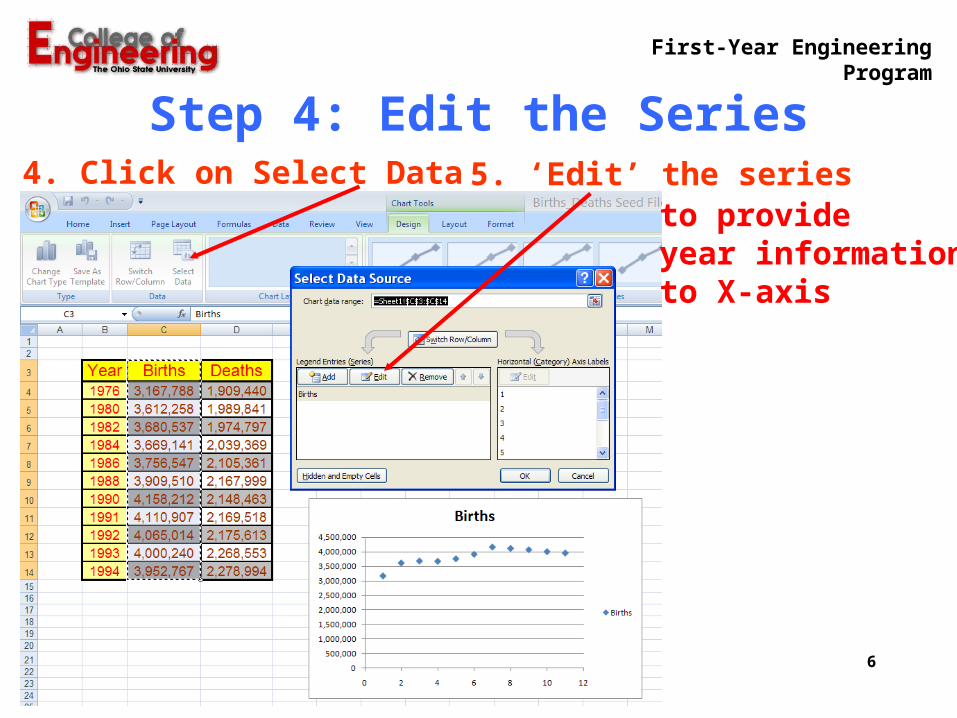
Step 4: Edit the Series4. Click on Select Data 5. ‘Edit’ the series
to provideyear informationto X-axis

First-Year Engineering Program
7Autumn 2009
Step 5: Continue5. Add X-Axis Information
Click here and then select x-axis values(Year Column Values)
First-Year Engineering Program
8Autumn 2009
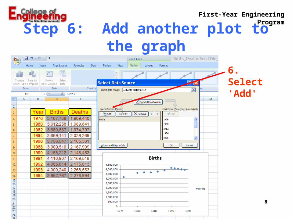
Step 6: Add another plot to the graph
6. Select 'Add'

First-Year Engineering Program
9Autumn 2009
Step 7: New Series Information
Set Series Name (Deaths)Set X-Axis
Values (Year values)
Set Y-Axis Values (Death values)

First-Year Engineering Program
10
Step 8: Formatting the Graph
6. Select Layout
Add Axis Labels and Chart Title to Produce
Autumn 2009

First-Year Engineering Program
11Autumn 2009
Scatter Plot of Example Data
First-Year Engineering Program
12Autumn 2009
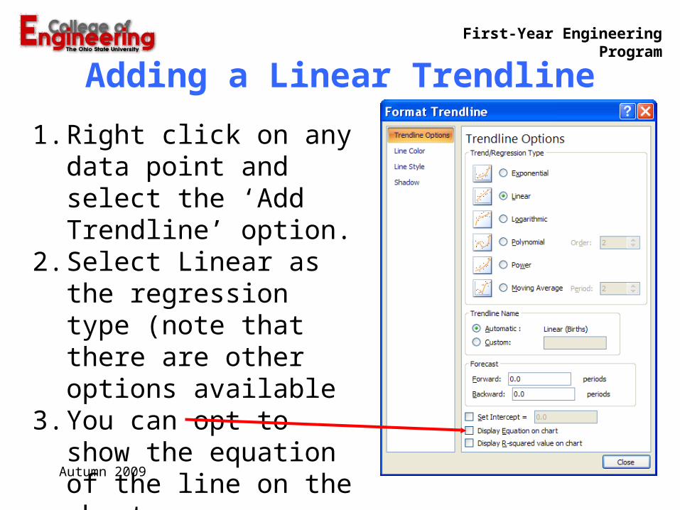
Adding a Linear Trendline
1. Right click on any data point and select the ‘Add Trendline’ option.
2. Select Linear as the regression type (note that there are other options available
3. You can opt to show the equation of the line on the chart
First-Year Engineering Program
13
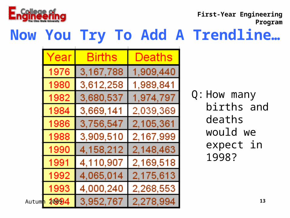
Now You Try To Add A Trendline…
Q: How many births and deaths would we expect in 1998?
Autumn 2009
First-Year Engineering Program
14Autumn 2009
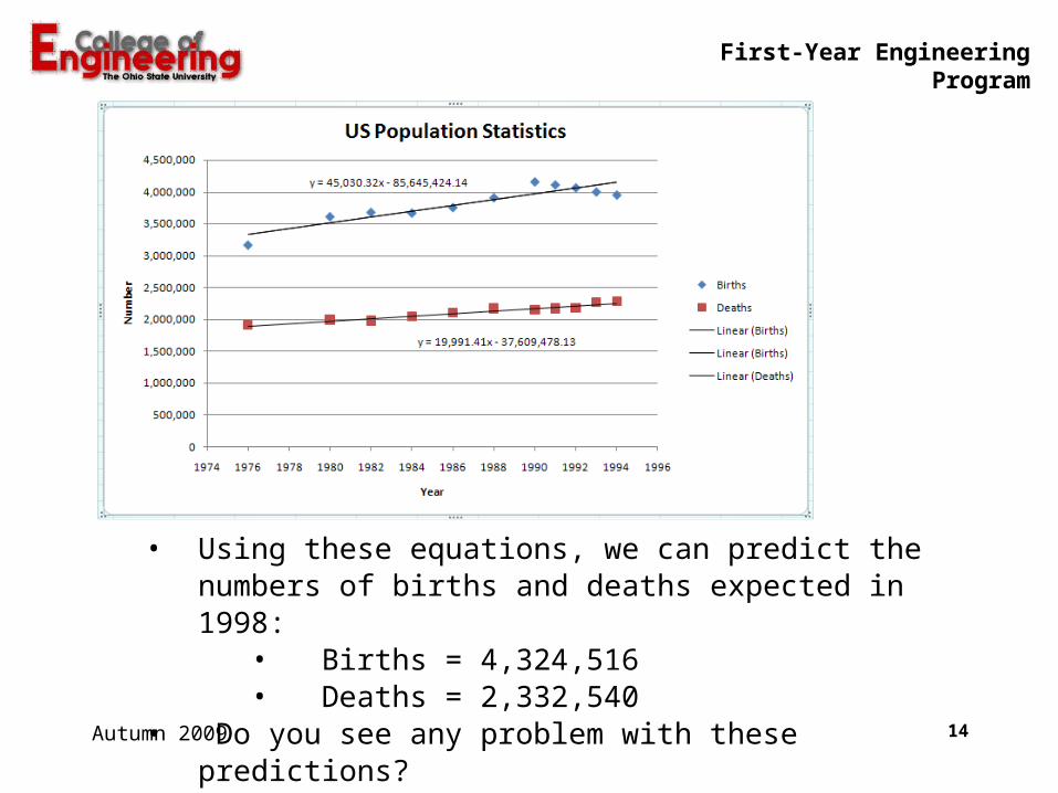
• Using these equations, we can predict the numbers of births and deaths expected in 1998:
• Births = 4,324,516• Deaths = 2,332,540
• Do you see any problem with these predictions?
First-Year Engineering Program
15Autumn 2009
Editing Excel Graphs
• Once a graph has been created by Excel you may need to edit a legend, title, label, etc.
• Place the cursor over the item to be edited and press the right mouse button and a menu will appear (Format or Clear)
• Choosing Format should allow you to edit the graph feature.

First-Year Engineering Program
16Autumn 2009
Copying Excel Charts and Tables into Word
• Select the Graph or Chart• Right click and select copy OR press
ctrl-C (shortcut).• Select the area in the Word document
where you want to place the chart or table
• Right click and select paste OR press ctrl-V (shortcut)
First-Year Engineering Program
17Autumn 2009
How to control the display of significant figures in Excel
In order to apply Significant Figure rules in Excel follow the steps below:•Select the cell(s) for which you
want to change the number presentation.
• Right-click and select 'Format Cells from the drop-down menu
NOTE: Excel keeps full precision of calculations internally.

First-Year Engineering Program
18Autumn 2009
This opens the dialog box shown here. The Decimal places selection allows you to limit the number of significant figures the cell will display.
How to control the display of significant figures in Excel
YOU NEED ONLY TO APPLY THE RULES TO THE CELLS IN WHICH FINAL RESULTS ARE CALCULATED!!!
First-Year Engineering Program
19Autumn 2009
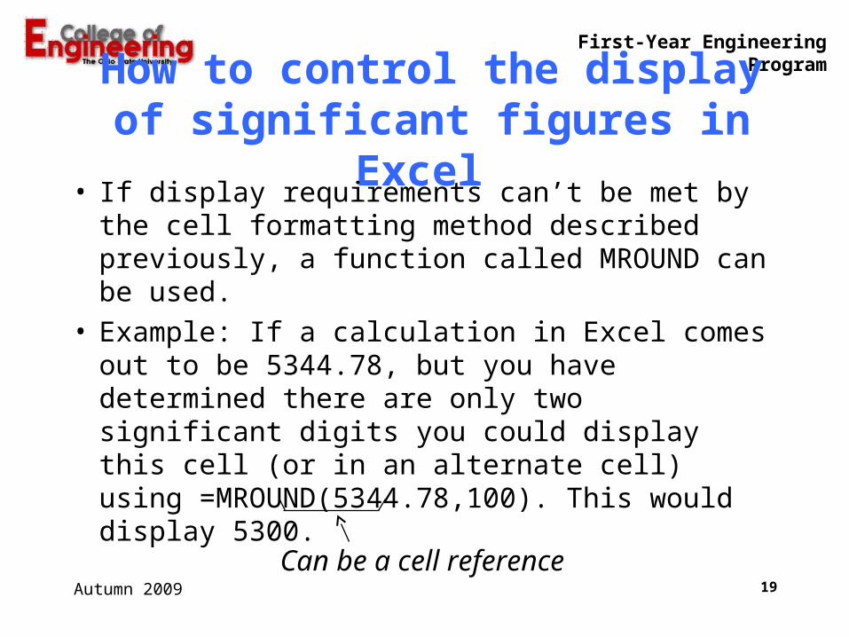
How to control the display of significant figures in Excel
• If display requirements can’t be met by the cell formatting method described previously, a function called MROUND can be used.
• Example: If a calculation in Excel comes out to be 5344.78, but you have determined there are only two significant digits you could display this cell (or in an alternate cell) using =MROUND(5344.78,100). This would display 5300.
Can be a cell reference

First-Year Engineering Program
20Autumn 2009
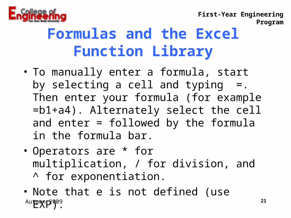
Formulas and the Excel Function Library
• Formulas are used to calculate values in a cell in a worksheet based on values stored in other cells and/or using the Excel function library.
• Examples of Excel functions include SUM, AVERAGE, MEDIAN, SIN, EXP, COSH and PMT.
• There are hundreds of functions available.
First-Year Engineering Program
21Autumn 2009
• To manually enter a formula, start by selecting a cell and typing =. Then enter your formula (for example =b1+a4). Alternately select the cell and enter = followed by the formula in the formula bar.
• Operators are * for multiplication, / for division, and ^ for exponentiation.
• Note that e is not defined (use EXP).
Formulas and the Excel Function Library

First-Year Engineering Program
22Autumn 2009
• To use the function library, click Insert…Function.
• An alternative is to type the function name in the cell or function bar.
• Remember to use proper cell referencing (described later)!
Formulas and the Excel Function Library

First-Year Engineering Program
23Autumn 2009
Insert…FunctionThe Excel function library contains hundreds of built-in functions.
From the 'Formulas' Tab select Insert Function. This allows you to select the function you need and to see how to use it.

First-Year Engineering Program
24Autumn 2009
Cell Referencing• The dollar sign ($) is used in cell
references to control what happens when you use the fill handle, or a straight copy and paste, to re-apply a formula in cell(s) in other rows and/or columns.• B12 – relative reference to value in cell
B12• $B12 – column fixed, but row can change• B$12 – row fixed, but column can change• $B$12- absolute reference to value in
cell B12
First-Year Engineering Program
25
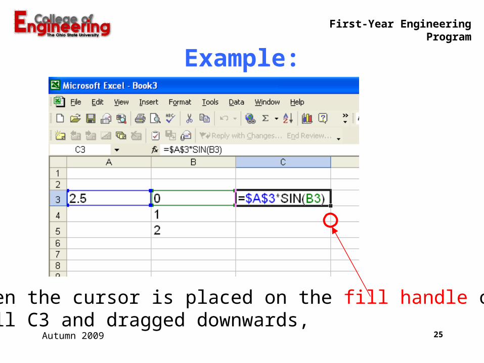
Example:
When the cursor is placed on the fill handle ofCell C3 and dragged downwards,
Autumn 2009
First-Year Engineering Program
26
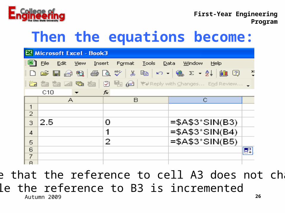
Then the equations become:
Note that the reference to cell A3 does not changewhile the reference to B3 is incremented
Autumn 2009

First-Year Engineering Program
27Autumn 2009
Cell Referencing Challenge
Enter a formula in cell B2 so that it can be dragged down and across to create this multiplication table
First-Year Engineering Program
28Autumn 2009
Challenge Answer
•If you entered =$A2*B$1, then you know most everything you’ll need to know about cell referencing!

First-Year Engineering Program
29Autumn 2009
Another ExampleCreate an Excel worksheet to plot the following function:
x(t) = 10 exp(-0.5t) sin(3t +2)over the range 0 t 20 seconds as a scatter plot at 1 second intervals.
Expected Result
x(t) = 10 exp(-0.5t) sin(3t +2)
-8
-6
-4
-2
0
2
4
6
8
10
0 5 10 15 20
t (sec)
x(t)
x(t)
First-Year Engineering Program
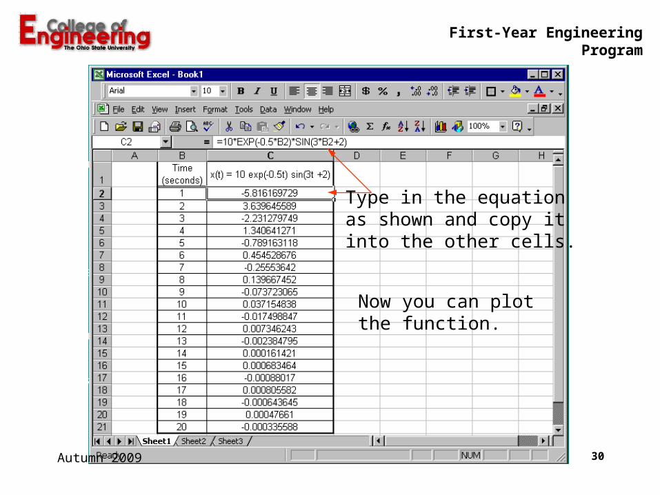
30
Type in the equation as shown and copy itinto the other cells.
Now you can plotthe function.
Autumn 2009

First-Year Engineering Program
31Autumn 2009
Assignment
•Refer to syllabus


