Fitting curves and surfaces to point clouds in the presence of obstacles SimonFl¨ory Geometric Modeling and Industrial Geometry Research Group, Vienna University of Technology, Wiedner Hauptstraße 8-10, A-1040 Wien, Austria Abstract We consider the problem of fitting B-spline curves and surfaces to point clouds in the presence of obstacles constraining this approximation at the same time. Therefore, we describe the fitting problem as optimization problem and employ an iterative procedure to solve it — the presence of obstacles poses constraints on this mini- mization process. We examine two families of obstacles: first, the point cloud itself is interpreted as obstacle, e.g. to reconstruct any apparant boundaries of the data set. Second, we define arbitrary regions the fitting must not penetrate. We discuss several numerical aspects of this constrained optimization and present experimental results for B-spline curve and surface fittings in the presence of obstacles. Key words: Curve fitting, Surface fitting, Obstacles, Constrained optimization, Surface trimming 1 Introduction The wide spread use of 3D laser scanning technology offers various possibil- ities to digitize real world objects and further process their virtual models on computers. One of the most common representation methods for the ac- quired measurement data stores a high number of surface sample coordinates, often denoted to as the point cloud. Data processing knows an ever increasing number of ways to deal with such a discrete point set: noise removal, mesh generation or registration to name only a few. A topic of special interest is to reduce the amount of information represented by the numerous elements of such a data set and smooth the point cloud at the same time. For this purpose, a curve or surface is fitted to the point set and used to represent the Email address: [email protected](Simon Fl¨ ory). Preprint submitted to Elsevier Science 25 April 2008
Transcript
Fitting curves and surfaces to point clouds in
the presence of obstacles
Simon Flory
Geometric Modeling and Industrial Geometry Research Group, Vienna Universityof Technology, Wiedner Hauptstraße 8-10, A-1040 Wien, Austria
Abstract
We consider the problem of fitting B-spline curves and surfaces to point clouds in thepresence of obstacles constraining this approximation at the same time. Therefore,we describe the fitting problem as optimization problem and employ an iterativeprocedure to solve it — the presence of obstacles poses constraints on this mini-mization process. We examine two families of obstacles: first, the point cloud itselfis interpreted as obstacle, e.g. to reconstruct any apparant boundaries of the dataset. Second, we define arbitrary regions the fitting must not penetrate. We discussseveral numerical aspects of this constrained optimization and present experimentalresults for B-spline curve and surface fittings in the presence of obstacles.
The wide spread use of 3D laser scanning technology offers various possibil-ities to digitize real world objects and further process their virtual modelson computers. One of the most common representation methods for the ac-quired measurement data stores a high number of surface sample coordinates,often denoted to as the point cloud. Data processing knows an ever increasingnumber of ways to deal with such a discrete point set: noise removal, meshgeneration or registration to name only a few. A topic of special interest isto reduce the amount of information represented by the numerous elementsof such a data set and smooth the point cloud at the same time. For thispurpose, a curve or surface is fitted to the point set and used to represent the
Preprint submitted to Elsevier Science 25 April 2008
measurement data henceforth. Less surprisingly, both curve and surface fit-ting are closely related and build upon the same basic considerations. Due totheir universality, free-form curves and surfaces are a popular choice as fittingentities and we focus on fittings with B-spline curves and surfaces below.
Conventional approaches in curve and surface fitting aim for an approximationof the shape represented by the point cloud. Often, this process is exposed toconstraints of abstract nature to ensure mathematical properties of the finalsolution. In our work, we let real world obstacles influence the fitting by meansof restricting the solution space for the final result. Within this context we areable to address several challenging tasks: boundary reconstruction of pointclouds, computation of fittings avoiding certain forbidden regions, computa-tion of hulls for moving objects and surface trimming to name only a few. Inachieving these goals, the main contributions of this work comprise the for-mulation of linear constraints induced by real world obstacles that integratewell with existing fitting algorithms. In detail, we consider the point clouditself as obstacle and subsets of the plane or space the final fitting must avoid.Moreover, we discuss numerical issues of the arising constrained optimizationproblem (suitable classes of algorithms and primal vs. dual solution).
The remaining parts of our paper are organized as follows. After a review ofrelated literature we describe the general fitting problem and develop con-straints once for a boundary approximation of the point set and second formore general obstacles. Subsequent to a short excursion to relevant topics ofconstrained optimization theory, several examples show applications of theproposed algorithm and discuss a handful of numerical properties.
1.1 Related Work
Piecewise parametric functions have been used in curve fitting of point cloudsfor a long time. In one of the first works on this topic, (Cox, 1971) employs aleast-squares method, an error metric still popular today, to fit scattered data.A major challenge in curve fitting, if compared to a univariate function ap-proximation, is to define those samples on the fitting entity the approximationerror is measured in. If the data points are ordered, the chordal length methodor the centripetal method (see e.g. (Hoschek and Lasser, 1993)) could be usedfor parametrization. (Hoschek, 1988) tackles the problem of unordered targetdata with an iterative method of intrinsic parametrization and approximatesthe foot point computation by a first order term. Approximations of higherorder (Saux and Daniel, 2003; Hu and Wallner, 2005) or an accurate foot pointcomputation (Hoschek and Lasser, 1993) in each step are subject of discussionas well. Once these foot points have been obtained, the distance function to thecurve is approximated. The most popular technique computes the squared dis-
2
tance from the data points to the foot points (Plass and Stone, 1983; Hoschek,1988; Goshtasby, 2000). (Blake and Isard, 1998) improve these approaches bymeans of convergence properties and utilizes the squared distance from thedata point to the tangent plane in the foot point as error term. Recently,(Wang et al., 2006) give an thorough overview of existing curve fitting meth-ods and describe an algorithm based on a second order approximation of thesquared distance function to solve the curve fitting problem.
The problem of surface fitting has been addressed for years as well (see e.g.(Hayes and Halliday, 1974)) and has drawn a certain amount of attention inrecent years. (Dierckx, 1993) give a comprehensive overview of curve and sur-face fitting techniques (scattered data fitting, mesh fitting and data smooth-ing) and is a good starting point for references to the older literature. (Dietz,1995) extend the existing least-squares approximations and discuss the use ofadditional smoothing and regularization terms. (Greiner and Hormann, 1996)consider the surface reconstruction with hierarchical tensor product B-splinesurfaces and (Diebel et al., 2006) apply a Bayesian method for probable sur-face reconstruction. The literature on this topic is extensive and we want toround up the review and refer to two recent publications (Weiss et al., 2002;Wang et al., 2006) and the references therein.
Constrained curve and surface design is a widely investigated topic in com-puter aided geometric design. Given a set of data points, side conditions havebeen imposed on interpolation methods with cubic splines and rational cu-bics to handle obstacles (Opfer and Oberle, 1988; Meek et al., 2003). Theconstrained approximation of point sets with Bezier or B-spline curves (cf.(Rogers, 1989; Bercovier and Jacobi, 1994)) may have various aims in mind,such as increasing the quality of the final fitting, simplifying it or ensur-ing certain geometric properties of the solution. Especially the latter taskis addressed in detail in (Hoschek and Kaklis, 1996) where properties suchas convexity and monotony of a final approximation are discussed. Certainshape preserving criterias or restrictions on the class of surfaces employedfor approximation pose constraints to fitting problems as well, e.g. in recon-structions of developable surfaces (Pottmann and Wallner (1999)). In ReverseEngineering, it is of special interest to reconstruct geometric primitives frommeasured data. In (Benko et al., 2002), various constraints are considered formultiple fittings of geometric objects, which are handled in a modified Newtoniteration. Further constrained methods in Reverse Engineering are surveyedin (Varady and Martin, 2002) and (Fisher, 2004). Besides these theoreticalconstraints, our special focus is on side conditions derived from real world ob-stacles. (Myles and Peters, 2005) construct splines of prescribed smoothnessobliged to stay in a channel with piecewise linear boundaries. In (Liu et al.,2005), a combination of surface fitting and registration based on a squared dis-tance minimization algorithm is discussed and applied to constrained reverseengineering of CAD models. Especially for registration, (Huang et al., 2006)
3
describe the local, simultaneous, penetration free alignment of multiple datasets as constrained optimization problem. (Lin and Wang, 2002) tightly bor-der planar point clouds resembling curves by B-spline interpolation of theirboundary points. In (Flory and Hofer, 2008), curve fittings are constrainedto happen on a smooth parametric surface. This main constraint is extendedby curve boundary approximations that represent simplified cases of what wewill discuss in the following. Furthermore, it is a common problem in motionplanning to deal with obstacles, see (Latombe, 1991).
2 Constrained curve and surface fitting
Let P = {pk ∈ Rd : k = 1, . . . , n} denote a set of unordered points in the plane(d = 2) or Euclidean three space (d = 3). Fitting a curve in the plane andfitting a surface in space to such a point cloud are closely related topics. Forthe ease of discussion, we will concentrate on the curve case in the followingand point out differences to the surface case where necessary.
2.1 General curve fitting
We choose to carry out the fitting (or approximation) of P with a parametriccurve x : R → R2, u → x(u). For now, we assume that x is closed anddoes not exhibit any self-intersections (we are going to show ways to deal withmore general approximating curves in Sec. 2.2 and 4). Furthermore, let d(x,p)denote the signed distance of a point p ∈ R2 to x. Then, the curve x is saidto fit P in a least-squares sense if it minimizes the sum of squared distancesfrom each element pk ∈ P to x,
n∑k=1
d2(x,pk) + ω · r. (1)
Here, r resembles a regularization term weighted by a factor ω, on whichwe will give motivation and details later on (see Sec. 4). Please note thatby minimizing the squared distance function we avoid any handling of thedistance function’s sign.
Common approaches tackle the optimization problem of Equ. (1) in an itera-tive way. For the current location of the fitting curve x, the squared distancefunction d2 from x is described approximately. Usually, this is done for eachdata point (or the corresponding closest point on x); an updated position ofx is obtained by minimizing the sum over all these approximated distancefunctions. Details on approximations of the squared distance function are dis-
4
Fig. 1. (Left) A classical least-squares curve fitting results in a balance of residues.(Middle) A point cloud resembling a self-intersecting shape is — due to its dis-crete nature — interpreted as not self-intersecting but with several interior regions.(Right) Open curve shape approximation.
cussed in the literature, for example (Wang et al., 2006) gave a thouroughoverview recently.
So far, the fitting problem and its roughly outlined solution have been de-scribed for any general parametric curve. However, we want to get more spe-cific about the employed curve type. As stated in the introduction we willuse B-spline curves as fitting curves. Assuming that knots and degree of sucha B-spline curve are fixed, we write x(u) =
∑mi=1Ni(u)di, where Ni(u) are
the B-spline basis functions and di ∈ R2 describe the curve’s control points.Accordingly, we denote by xc(u) =
∑mi=1Ni(u)(di + ci) any updated position
of x. For convenience, we will summarize the displacements ci into a singledisplacement vector c. With this notation in mind, we are able to describe ageneral fitting algorithm.
(1) Assign each data point pk a parameter value uk such that x(uk) is theclosest point of pk on x(u).
(2) Describe the current fitting error of x w.r.t. P . Therefore, approximatethe squared distance function of x to P in the foot points x(uk).
(3) Compute the displacements c of the fitting curve’s control points by min-imizing this approximation error. If the fitting is of satisfactory quality,stop, or continue at step 1, otherwise.
Commonly used stopping criterias ask for the number of iterations exceedinga pre-defined value or demand for the averaged squared distances from P tox to fall below a user-defined threshold.
2.2 Boundary approximation
Considering the point cloud P , a fitting as outlined above will yield a finalapproximation following the shape of the point cloud by means of a balancein residues. Loosely speaking, if we assume that the point cloud exhibits somewidth, the curve will pass through the middle of the point cloud stripe, suchthat there are points to both sides of x (see Fig. 1, left). In the following, we
5
are interested in achieving an opposite effect and aim at approximating anyapparant boundaries of the point cloud.
Let x be a closed parametric curve (in the plane) or a surface (in 3D) withoutself intersections and d(x,p) the signed distance function to x defined in sucha way that d(x,p) < 0 holds for all points p ∈ D, whereas D denotes thedomain bounded by x. By considering the sign of the distance function, weare able to define a boundary reconstruction of a point cloud: x approximatesthe outer or inner boundary of P if x minimizes Equ. (1) and d(x,pk) < 0 ord(x,pk) > 0 holds for all pk ∈ P .
In the following we will explicitely exclude fittings with self intersecting curvesor surfaces. This doesn’t pose any limitations to our succeeding considerationsif we consider that the notion of a self intersecting point cloud is hard to grab.Given that a point cloud is a discrete set of data points, such a point cloudmay be seen as a non self-intersecting point set at the same time, exhibiting awell defined outer boundary and an inner boundary consisting of several nonconnected components (see Fig. 1, middle). Please note, that for some pointclouds, there might be no meaningful inner boundary at all (see Fig. 1, right,and Fig. 8, bottom right).
For fittings of point clouds resembling an open curve shape, the above defini-tion doesn’t make sense as for an open fitting curve no inner or outer regioncan be defined. Nevertheless, such an open shape might be seen as specialcase of a point cloud with no inner boundary. Thus, we approximate the outerboundary of such a point cloud with an artificially closed approximation curveand restrict the parameter space of the final fitting curve x to those parts ofthe boundary we wanted to approximate (see Fig. 1, right).
We have seen that the problem of curve fitting can be turned into an opti-mization problem that is solved with an iterative procedure. Approximatingthe boundary of a point cloud imposes constraints on this optimization prob-lem, e.g. the outer boundary of a point set is reconstructed by that curveminimizing the constrained optimization problem,
minimizen∑
k=1
d2(x,pk) + ω · r
subject to d(x,pk) < 0 ∀pk ∈ P.(2)
For a solution of the unconstrained minimization problem we approximatedthe squared distance function by quadratic functions. Following the same idea,we will now derive suitable approximative side conditions from the definitionof boundaries introduced above. For an approximation of the outer boundary,d(x,pk) < 0 must hold for all pk ∈ P . d(x,pk) describes the signed distancefrom pk to x, which defines a foot point x(uk) such that |d(x,pk)| = ‖x(uk)−pk‖. By computing the first order Taylor approximation of d in that foot point
6
x(uk), we obtain
dk(x,p) ≈ d(x(uk)) +∇pd(x(uk))T · (p− x(uk)).
As d(x(uk)) = 0 holds and ∇pd coincides with the outward normal vectorn(uk) in x(uk), we approximate the constraint d(x,pk) < 0 for a data pointpk by
(pk − x(uk))T · n(uk) < 0, (3)
which basically means that we replace x by its tangent in the foot point andrequire pk to be located on the opposite side of the tangent the normal pointsto.
In the course of optimization, x will get displaced to better approximate thepoint cloud. Thus, the foot point x(uk) and the normal n(uk) will change asthey depend on the current shape of the fitting curve, given by the currentcontrol points (summarized in a single vector d). Precisely speaking, for ourchoice of B-splines as approximating curves, x(uk) and n(uk), and thus thewhole left hand side of Equ. (3),
l(d) = (pk − x(uk(d),d))T · n(uk(d),d),
depends on the control points in a highly non-linear way. We are going toconsider two ways to deal with this dependancy. Our first approach will simplyregard the foot points as fixed and thus ignore this relation at all,
(pk − xc(u0k))T · n(u0
k) < 0. (4)
Here, superscript index 0 labels values at the beginning of the current iteration.
Another way to deal with this dependancy is to linearize l(d),
l(d) ≈ l(d0) +∇dl(d0)T · (d− d0).
For the computation of the gradient∇dl, partial derivation of l(d) with respectto di yields
∂l
∂di
(d) = −Ni(uk(d)) · n +∂n
∂di
· (pk − x).
Here, Ni describe the B-spline basis function again. Let J denotes the rotationby π/2 turning x(uk) into the outward oriented normal vector. Then, ∂n
∂di=
J x ·(
∂uk
∂di
)T+Ni ·1 with 1 ∈ R2×2. The partial derivatives of uk(d) are defined
in an implicit way by the condition that in a closest point x(uk) the tangentx(uk) is perpendicular to the connecting vector from x(uk) to pk,
Fig. 2. (Left) At the end of an iteration, the data points lie on the opposite side ofthe tangent the normal points to. (Right) For smooth bounded general obstacles,all curve samples sk within a certain distance (denoted by the dashed line) to anobstacle’s boundary are constrained to be located outside any forbidden region.
Derivation of this expression with respect to di yields
∂uk
∂di
(d) = − Ni · (x− pk) +Ni · xxT · (x− pk) + xT · x
.
By requiring the linear approximation of l(d) to be negative (compare Equ. (3)),we obtain for c = d− d0 the linear constraints of the second type,
∇l(d0)T · c < −(pk − x(u0k))T · n(u0
k). (5)
These considerations are generalized to the three dimensional surface casestraight forward. For a B-spline surface x(u, v) =
∑m′
i=1N′i(u, v)di, the normal
vector in a foot point x(uk, vk) may be computed by the cross product of thederivatives along the parameter lines, n(uk, vk) = xu(uk, vk) × xv(uk, vk). Asbefore, the derivatives of u(d) and v(d) with respect to dj for the partialderivatives of l(d) are defined implicitely by the conditions for a foot point ofthe shortest distance between a sample pk and a surface x, which read in thesurface case as
xTu (uk, vk) · (pk − x(uk, vk)) = 0 and xT
v (uk, vk) · (pk − x(uk, vk)) = 0.
For the ease of reading, we omit the final expression for ∂l∂di
and ∂n∂di
which areobtained similar to the curve case.
2.3 General obstacles
Going beyond the boundary approximation of point clouds, we might considersubsets {Oj} ⊆ R2 the final approximating curve x of a point cloud P isobliged to avoid. Given that each region Oj is bounded by a smooth curveoj, a feasable fitting in the presence of such obstacles can be defined in a
8
way closely related to the previous section on boundary reconstruction. Ifwe assume that the distance function to oj is negative for points inside anobstacle, a curve x does not penetrate any Oj if d(oj, s) > 0 holds for alls ∈ x. Contrary to the previous considerations for boundary approximation,this definition naturally holds for closed and open curves, with and withoutself intersections.
For applications, we will weaken this condition. We discretize the curve x indense samples S = {sk} and ask for d(sk) > 0 for all sk ∈ S. Then, a curvefitting in the presence of general obstacles yields constraints of the same typeas for the boundary case,
(fOk − sk))T · nO
k > 0, (6)
where fOk is the foot point of the shortest distance from a sample point sk to
the closest obstacle Ok and nOk the normal in that foot point. In an adapted
sense, the same considerations for the dependancy of any samples, foot pointsand normals to the current location of x apply.
3 Constrained Optimization
So far, we described an iterative solution for the curve fitting problem alongwith approximative linear constraints induced by specific real world obstacles.In this section, we are going to restate the boundary approximation problemof Equ. (7) with above results and show ways to solve it. As noted in Sec. 2.1,the sum of squared distances in the objective function can be approximated assum over quadratic terms Qk(c). Then, by making use of the approximativeside conditions of Sec.2.2, we may write our constrained optimization problemin the form,
minimizen∑
k=1
Qk(c) + ω · r(c)
subject to Equ. (4) or Equ. (5).
(7)
This minimization problem is solved at each iteration of the algorithm de-scribed in Sec. 2.1 to obtain an updated position of the approximating curvex. As we are going to choose a regularization term r(c) quadratic in theunknown displacments c (see Sec. 4), the objective function of Equ. (7) isquadratic in c. If there were no constraints, a minimum would be found bysolving a system of linear equations. However, we face constraints linear in c.
There are basically two families of algorithms solving quadratic programmingproblems with linear constraints (see e.g. (Nocedal and Wright, 1999)). Activeset methods have been the most important technique for a long time. They
9
deal with the constraints by estimating and continuously updating a set ofcurrently active side conditions. The generalization of Interior point methodsto quadratic programs, which in contrast avoid the boundary of the feasibleregion, provided a second powerful method for the solution of quadratic pro-grams. While Active set methods are, in general, better suited for smallerscaled problems, Interior point methods are widely used for larger scaled op-timization tasks.
Considering that the dimension of c in Equ. (7) is only two or three timesthe number of control points of x this optimization problem is rather smallscaled from the viewpoint of optimization. However, the number of constraintsmay equal the possibly big number of elements in the point cloud. Thereforeit might be favorable to solve the dual problem as it reduces the complexityof the constraints while increasing the dimension of the problem at the sametime.
If we write the primal quadratic program of Equ. (7) in a more general form,
minimize 12cTHc + tT c H ∈ R3m×3m, c, t ∈ R3m
subject to Ac− b ≤ 0 A ∈ Rn×3m, b ∈ Rn,(8)
its Lagrange function is given by
L(c, λ) = 12cTHc + tT c + λT (Ac− b) λ ∈ Rn.
The dual problem is then defined as finding the maximum of the dual function
q(λ) := infc∈R3m
L(x, λ) = −12λTQλ− qTλ− 1
2tTH−1t,
where we write in short Q = AH−1AT and q = AH−1t + b. Therefore, thedual problem of the primal one in Equ. (8) is yet another quadratic program,
maximize − 12λTQλ− qTλ
subject to λ ≥ 0.(9)
The solution of the primal problem is given as the minimal argument of L(x, λ)for λ fixed, thus c = −H−1(t+ATλ). As for our optimization task strong du-ality holds, it could be favorable to focus on the dual problem. In the followingsection, we will examine experimentally which method shows best performancefor our task of curve and surface fittings in the presence of obstacles.
4 Experiments and results
Now, as we have set up a theoretical framework for curve and surface fit-tings in the presence of obstacles, we want to apply these considerations to
10
Fig. 3. Reconstruction of a point cloud’s boundary: initial setup (left) and finalapproximation after 10 iterations (right).
a handful of examples. We describe various experiments showing the methodin use — in particular, we will address any remaining open questions suchas in how far the two proposed constraints of Equ. (4) and Equ. (5) showdifferent performance and what is the best optimization technique to tacklethe emerging constrained optimization problems. As basic fitting algorithm,we employ the method of Squared Distance Minimization, which builds uponsecond order Taylor approximation of the squared distance function in thefoot points x(uk) of the shortest distances from the elements of P to x (for adetailed description of this method, see (Wang et al., 2006)).
Another issue that needs to be addressed are details on the regularizationterm in Equ. (7). As an optimal solution in a mathematical sense does notnecessarily mean a visually appealing solution (e.g. strong oscillations mightoccur), a simplified measure for the bending energy,
r(c) =∫‖xc(u)‖2du,
is added to the problem’s objective function. Please note that this expressionis quadratic in c. Details on the weighting factor ω (which is halved aftereach iteration step) can be found along with other relevant key figures of thefollowing examples in Tab. 1. The algorithms for curve fittings were imple-mented in a Matlab environment whereas the surface fitting code was writtenin C/C++. All results were obtained on a AMD Sempron Processor 3100+computer.
Example 1 The first example is a simple application of the described algo-rithm and approximates the boundaries of a set of data points in the plane.The point cloud in this experiment was, as those of several succeeding ex-amples, artifically created. For this purpose, an auxilary B-spline curve wassampled in a user specified number of points which were then displaced in nor-mal direction by distances drawn from a Gaussian distribution. In Example 1,the approximating B-spline curve was cubic and counted 13 control points. By
11
Fig. 4. Fitting a cubic B-spline curve to a point cloud in the presence of four gen-eral obstacles. For three different initial setups (top row), the corresponding finalapproximations after 25 iterations (bottom row) are shown.
using the second type linear constraints of Equ. (5), the inner and the outerboundary of the point cloud were approximated with an Active set method;both results were summarized in a single plot in Fig. 3 (right).
Example 2 The second example exhibits a curve fitting constrained by foursmooth bounded forbidden regions. In a preprocessing step, an approximateddistance field from the obstacles’ boundaries was computed (applying thesweeping algorithm described in Tsai (2002)), which took 15.6 seconds on a[0, 1]×[0, 1] grid with a resolution of 0.01. At each iteration, the distance valuesof this discretization were used to determine those sample points sk ∈ xc(u)close to a forbidden region (minj d(sk, Oj) < 0.04). For these samples, linearconstraints of the second type were added to the optimization problem. Fig. 4shows three approximations of the same setup (with respect to point cloudand obstacles) but with distinct differing initial positions of the approximatingB-spline curve. As the results indicate, are the fittings barely influenced bythe starting configuration.
For most of the experiments presented here, the linear constraints have beendeactivated in the first 3 to 5 iterations (the exact number is given in brack-ets in the column holding the number of iterations in Tab. 1). This way, thefitting curve first approximates the point cloud before taking any obstaclesinto account - a strategy improving the stability of the method significantly.Please note, that the final solution of an approximation avoiding certain re-gions depends on the actual location of the fitting curve in the moment whenthe constraints are actived for the first time and is thus not unique. Obsta-cles inside the domain bounded by a closed approximating curve will remain
12
Fig. 5. (Left column) A boundary approximation with constraints obtained by lin-earizing any dependancy on the foot points. (Top row) If applying solely constrainediterations, this method (solid line) performs better than that ignoring any relation(dashed line). (Bottom row) Unconstrained iterations in the beginning cancel anyadvantage.
inside, the same applies to obstacles outside.
Example 3 In Sec. 2.2 we derived two types of linear constraints for a pointcloud’s boundary approximation. If the side conditions are active from thevery beginning, the constraints of the second type obtained by linearizationlet us expect faster convergence as the curve doesn’t fit the point set’s shapewell and thus causes relevant changes of the foot points. In contrast, if we firstfit the point cloud with some unconstrained iterations roughly, using the moresophisticated constraints may not pay off as most of the curve’s displacementhappens in normal direction and thus leads to only minimal changes in thefoot points. In Fig. 5, we compare both types of constraints in the course ofan outer boundary approximation of a point cloud. The inital setup was thesame for all optimizations, as well as the final fittings were of similar quality.If the side conditions are active from the beginning, the linearized constraints(solid line) outperfrom the constant constraints (dashed line), both in termsof decrease of points in the forbidden region and in terms of the averageapproximation error,
εavg =1
n
n∑i=1
‖x(uk)− pk‖.
However, if we apply 10 unconstrained iterations steps first, both approachesshow similar performance, with the constant type performing even slightlybetter in the example at hand. Considering that the additional computation
13
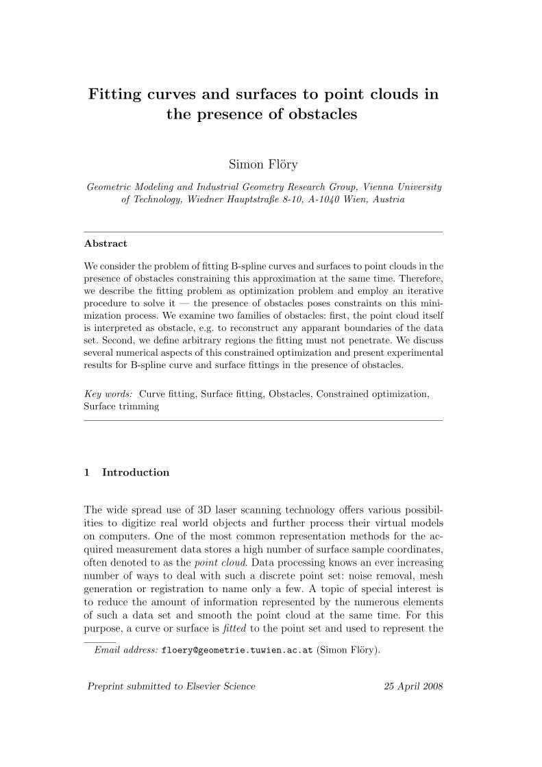
Fig. 6. (Top) Boundary approximation of a point cloud counting 500 elements bysolving the dual problem. (Bottom left) An Active set method shows faster con-vergence than an Interior point method. (Bottom right) Solving the dual problemtakes more and more time for a growing number of points.
time for the second type of constraints is minimal, one might favor the secondapproach applying a fitting without side conditions first. This is because thecosts of an unconstrained optimization step are considerably lower than thatof a constrained minimization.
The condition that the approximating curve is not self-intersecting proofedto be important for the theoretical work in Sec. 2. If we choose the initialposition of the curve manually, this requirement can be fulfilled easily. If weobtain it in an automatic way, such as in parts for this example, we canavoid self-intersections in the course of optimization by choosing a high initialregularization weight ω and decrease it carefully.
Example 4 Given the boundary approximation problem of Fig. 6 we dis-cuss two further numerical aspects of unconstrained optimization. First, asActive set methods are said to perform better than Interior point methods forsmall and medium scaled problems (such as our fitting problems), we wantto examine which one of the two algorithm classes suits our purposes best.Though we are aware of the fact that a thorough investigation of this task isout of scope of our work, we compared Matlab’s standard solver for medium
14
Fig. 7. Boundary approximation of a point cloud in 3D. A CAD model is sampled,exposed to simulated shakings (left) and approximated by a B-spline surface closedin one parameter direction (right).
scaled problems (an Active set method, cf. (Gill et al., 1981)) with a Matlabimplementation of a recently proposed Interior point method (Absil and Tits,2007). Fig. 6 (bottom, left) visualizes the convergence speed of both algorithms(with the second type of boundary constraints active from the beginning) overa period of 15 iterations. This comparison confirms advantages of the Activeset method.
For a second numerical issue we notice that the dimension of the unknown dis-placement vector c is small, whereas the number of linear constraints growswith the size of the point cloud. Thus, as outlined in Sec. 3, it may be worthto address the dual problem which is larger scaled but shows more simple con-straints that can be tackled with specialized algorithms. In our framework, weapplied a solver for quadratic programs with only bound constraints (Neu-maier, 1998). However, we couldn’t observe any advantage in addressing thedual problem. We see two reasons for this: once, the increase in dimension isquite large when changing from the primal to the dual problem. Second, thedual problem shows worse condition than its primal counterpart.
Example 5 In another example, we want to illustrate the surface approxi-mation of a point cloud’s outer boundary. Within this context, we are goingto address a common problem in engineering. Consider the mechanical partsof an operating machine, thus exposed to vibrations. If we are in need of a hullfor such an object, we have to take into account all possible positions and wrapthem with a surface. For our example, we use the CAD model of a pipe (seeFig. 7) and sample its surface in approximately 3000 points. Then, we simulate
15
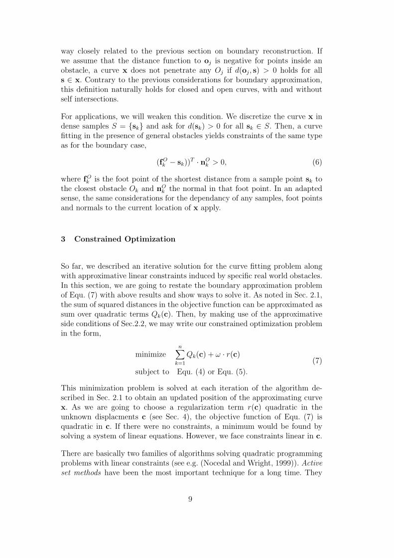
Fig. 8. (Top) Initial and final setup of a surface fitting in the presence of general ob-stacles. (Bottom) Some intermediate results: untrimmed initial surface, untrimmedfinal surface and parameter domain boundary approximation for trimming.
the shaking of operation by applying some random translations to this pointcloud, whereas translations in positive direction of two coordinate axis maybe observed more frequently. We summarize the relocated data points into asingle point set and compute an approximation of its outer boundary. TheB-spline surface is closed with respect to one parameter and counted 15× 22control points. The final result was trimmed such that the parameter domainranges from 0 to 1 in the closed parameter direction and was bounded bystraight lines in the other direction. In order to deal with the large number ofpoints (and thus constraints), only data points within a distance of 0.05 to theapproximating surface entered the optimization. Please note that we employedthis strategy of including only a subset of P for constraining the optimizationonly in this example. In all other experiments, each pk ∈ P contributed a sidecondition to the minimization.
Example 6 In this example, the point cloud results from digitizing an ob-ject with a 3D laser scanner. We place three geometric primitives (a sphere,a cylinder and a cube) close to the data set and ask for a B-spline surfacereconstruction avoiding these objects. For this purpose, we first fit a plane tothe point cloud, define the initial position of the control points on a rectan-gular grid thereon and distort these in normal direction. In order to prevent ashrinking of the approximating surface, we let it overlap the data set signifi-cantly and fix the outer frame of control points in the subsequent optimization.Then, we employ the algorithm of Sec. 2.3 to compute a surface fitting notpenetrating the obstacles. Contrary to Example 2, we didn’t discretize thedistance to the obstacles on a grid but sampled the obstacles boundary andadded constraints for the foot points of those samples on the approximating
16
Example Nr. points in P Iterations (constr.) ω Time (s)
1 500 10(3) 0.0001 3.0
2 200 25(5) 0.0001 14.5
3 1000 15(0) 0.001 16.4, 16.8
15(10) 0.001 13, 13.2
4 100 . . . 1000 15(0) 0.005 9.8, see also Fig. 6
5 60000 15(5) 0.04 277.3
6 5000 15(5) 0.01 208.5Table 1Configuration parameters and runtime information for the examples of Sec. 4.
surface. For a proper visualization, we trim the fitting B-spline surface to theeffective extent of the point cloud. Therefore, we determine the foot points ofthe point cloud’s elements on the final surface and consider the correspond-ing parameters in (u, v)-parameter space. There, the parameters form a pointcloud by themselves; the outer border of this point cloud is a good estimatefor the boundary of the trimmed surface. We approximate the extent of theparameters with a B-spline curve with the methods of Sec. 2.2 and let theresulting fitting curve define the boundary of parameters contributing to thetrimmed surface. Fig. 8 visualizes the final result of the constrained, trimmedsurface fitting.
At this point, we want to refer one more time to Tab. 1, in which we summa-rize information on the examples’ point clouds and their approximations. Thesecond column holds the number of elements of the point cloud. For Example4, the visualized boundary approximation and comparison of Active set andInterior point method was done for 500 data points, while the performance ofboth methods for a growing number of points was measured for point cloudswith sizes ranging from 100 to 1000 points. The third column gives the totalnumber of iterations to obtain the final solution, the numbers in brackets givethe share of any unconstrained iterations steps. For the timing values of Ex-ample 3, approximations with side conditions ignoring any dependancy on thefoot points come first. In general, if an example comprises more than a singleapproximation but Tab. 1 includes only a single value, the measured numberswere identical (iterations) or very similar (time).
5 Conclusions and future research
We presented an algorithm to fit a curve (in 2D) or a surface (in 3D) to a setof unordered points in the presence of obstacles. As obstacles, we considered
17
once the point cloud itself as constraint. Second, we restricted the approxima-tion to a subset of the plane or space. By adapting the idea of common fittingapproaches that interpret the fitting problem as optimization problem solvedin an iterative way, we derived constraints to this optimization from the obsta-cles under consideration. Basically, we presented two types of constraints, bothdealing with the dependancy of the constraints on the changing foot points ina different way. While the unconstrained fitting problem yields minimizationof a quadratic objective function, the introduced side considitions are linearin the unknown displacement of the curve. We discussed some questions con-cerning the solution of such a quadratic program with linear constraints andillustrated the way the algorithm works in various examples.
We see several directions our work on constrained fittings may be continued.The fact that we keep knot vector and number of control points of the ap-proximating B-spline curve or surface fixed poses certain limitations on theadaptiveness of the method. Thus it is of interest in how far existing solutionsfor the unconstrained case (cf. (Yang et al., 2004)) can be integrated into ourconstrained approximation framework to increase the flexibility of our algo-rithm. The error term describing the current approximation error poses furtherresearch challenges we hope to address in the future. Most approaches so faremploy approximations of the squared distance function, thus obtaining so-lutions in a least-squares sense. Least-squares fitting is known to be sensitiveto outliers, a problem that could be overcome by an approximation in the L1
norm, leading to non-smooth optimization problems.
Today, most point clouds forming the input to fitting problems originate from3D laser scanners. Such scanners, as every physical measurement device, ex-hibit distinct noise characteristics that can be determined in experiments anddescribed in a mathematical way. Knowledge about this noise can enter the ap-proximation process such that not the curve or surface with smallest distanceto the point cloud is computed but the most probable curve or surface, giventhe characteristic noise. We hope to address these issues in future research.
Acknowledgements
I would like to thank Helmut Pottmann for his valuable comments and sugges-tions throughout the development of this work and the anonymous reviewerfor their efforts to improve the paper. This research was supported by the Aus-trian Science Fund (FWF) as part of the projects P16002-N05 and P18865-N13and a Neumaier fellowship.
18
References
Absil, P.-A., Tits, A. L., 2007. Newton-KKT interior-point methods for indef-inite quadratic programming. Comput. Optim. Appl. 36 (1), 5–41.
Bercovier, M., Jacobi, A., 1994. Minimization, constraints and compositeBezier curves. Comput. Aided Geom. Des. 11 (5), 533–563.
Blake, A., Isard, M., 1998. Active Contours. Springer-Verlag New York, Inc.,Secaucus, NJ, USA.
Cox, M. G., 1971. Curve fitting with piecewise polynomials. IMA J Appl Math8 (1), 36–52.
Diebel, J. R., Thrun, S., Brunig, M., 2006. A Bayesian method for probablesurface reconstruction and decimation. ACM Trans. Graphics 25 (1), 39–59.
Dierckx, P., 1993. Curve and surface fitting with splines. Oxford UniversityPress, Inc., New York, NY, USA.
Dietz, U., February 1995. Erzeugung glatter Flachen aus Meßpunkten. Tech.Rep. 1717, Preprint Series, Department of Mathematics, Darmstadt TU.
Fisher, R. B., 2004. Applying knowledge to reverse engineering problems.Computer-Aided Design 36 (6), 501–510.
Flory, S., Hofer, M., 2008. Constrained curve fitting on manifolds. Computer-Aided Design 40 (1), 25–34.
Gill, P. E., Murray, W., Wright, M. H., June 1981. Practical Optimization.Elsevier.
Goshtasby, A. A., 2000. Grouping and parameterizing irregularly spaced pointsfor curve fitting. ACM Trans. Graphics 19 (3), 185–203.
Greiner, G., Hormann, K., 1996. Interpolating and approximating scattered3D-data with hierarchical tensor product splines. In: Mehaute, A. L., Rabut,C., Schumaker, L. L. (Eds.), Surface Fitting and Multiresolutional Methods.Vanderbilt University Press, pp. 163–172.
Hayes, J. G., Halliday, J., 1974. The least-squares fitting of cubic spline sur-faces to general data sets. IMA J Appl Math 14 (1), 89–103.
Lin, H., Wang, G., 2002. Interval b-spline curve evaluation bounding pointcloud. In: PG ’02: Proceedings of the 10th Pacific Conference on Com-puter Graphics and Applications. IEEE Computer Society, Washington,DC, USA, p. 424.
Liu, Y., Pottmann, H., Wang, W., August 2005. Constrained 3D shape recon-struction using a combination of surface fitting and registration. Tech. Rep.144, Geometry Preprint Series, Vienna Univ. of Technology.
Meek, D. S., Ong, B. H., Walton, D. J., 2003. Constrained interpolation withrational cubics. Computer-Aided Design 20 (5), 253–275.
Myles, A., Peters, J., 2005. Threading splines through 3D channels. Computer-Aided Design 37 (2), 139–148.
Neumaier, A., 1998. Minq - general definite and bound constrained indefinitequadratic programming.URL http://www.mat.univie.ac.at/∼neum/software/minq/
Nocedal, J., Wright, S. J., 1999. Numerical Optimization. Springer.Opfer, G., Oberle, H. J., 1988. The derivation of cubic splines with obstacles
by methods of optimization and optimal control. Numer. Math. 52, 17–31.Plass, M., Stone, M., 1983. Curve-fitting with piecewise parametric cubics. In:
SIGGRAPH ’83: Proc. of the 10th annual conference on Computer graphicsand interactive techniques. ACM Press, New York, NY, USA, pp. 229–239.
Pottmann, H., Hofer, M., 2003. Geometry of the squared distance function tocurves and surfaces. In: Hege, H.-C., Polthier, K. (Eds.), Visualization andMathematics III. Springer, pp. 223–244.
Pottmann, H., Leopoldseder, S., 2003. A concept for parametric surface fittingwhich avoids the parametrization problem. Comput. Aided Geom. Design20 (6), 343–362.