167
ORF555 / FIN555: Fixed Income Models Dami r Fi li povi´ c Department of Operations Research and Financial Engineering Princeton University Fall 2002

8/7/2019 Fixed Income Models
http://slidepdf.com/reader/full/fixed-income-models 1/167
ORF555 / FIN555:Fixed Income Models
Damir Filipovic
Department of
Operations Research and Financial Engineering
Princeton University
Fall 2002

8/7/2019 Fixed Income Models
http://slidepdf.com/reader/full/fixed-income-models 2/167
2

8/7/2019 Fixed Income Models
http://slidepdf.com/reader/full/fixed-income-models 3/167
Contents
1 Introduction 7
2 Interest Rates and Related Contracts 9
2.1 Zero-Coupon Bonds . . . . . . . . . . . . . . . . . . . . . . . . 9
2.2 Interest Rates . . . . . . . . . . . . . . . . . . . . . . . . . . . 11
2.2.1 Market Example: LIBOR . . . . . . . . . . . . . . . . 12
2.2.2 Simple vs. Continuous Compounding . . . . . . . . . . 12
2.2.3 Forward vs. Future Rates . . . . . . . . . . . . . . . . 13
2.3 Bank Account and Short Rates . . . . . . . . . . . . . . . . . 14
2.4 Coupon Bonds, Swaps and Yields . . . . . . . . . . . . . . . . 15
2.4.1 Fixed Coupon Bonds . . . . . . . . . . . . . . . . . . . 16
2.4.2 Floating Rate Notes . . . . . . . . . . . . . . . . . . . 162.4.3 Interest Rate Swaps . . . . . . . . . . . . . . . . . . . 17
2.4.4 Yield and Duration . . . . . . . . . . . . . . . . . . . . 20
2.5 Market Conventions . . . . . . . . . . . . . . . . . . . . . . . . 22
2.5.1 Day-count Conventions . . . . . . . . . . . . . . . . . . 22
2.5.2 Coupon Bonds . . . . . . . . . . . . . . . . . . . . . . 23
2.5.3 Accrued Interest, Clean Price and Dirty Price . . . . . 24
2.5.4 Yield-to-Maturity . . . . . . . . . . . . . . . . . . . . . 25
2.6 Caps and Floors . . . . . . . . . . . . . . . . . . . . . . . . . . 25
2.7 Swaptions . . . . . . . . . . . . . . . . . . . . . . . . . . . . . 29
3 Statistics of the Yield Curve 33
3.1 Principal Component Analysis (PCA) . . . . . . . . . . . . . . 33
3.2 PCA of the Yield Curve . . . . . . . . . . . . . . . . . . . . . 35
3.3 Correlation . . . . . . . . . . . . . . . . . . . . . . . . . . . . 36
3

8/7/2019 Fixed Income Models
http://slidepdf.com/reader/full/fixed-income-models 4/167
4 CONTENTS
4 Estimating the Yield Curve 39
4.1 A Bootstrapping Example . . . . . . . . . . . . . . . . . . . . 394.2 General Case . . . . . . . . . . . . . . . . . . . . . . . . . . . 44
4.2.1 Bond Markets . . . . . . . . . . . . . . . . . . . . . . . 45
4.2.2 Money Markets . . . . . . . . . . . . . . . . . . . . . . 46
4.2.3 Problems . . . . . . . . . . . . . . . . . . . . . . . . . 48
4.2.4 Parametrized Curve Families . . . . . . . . . . . . . . . 49
5 Why Yield Curve Models? 65
6 No-Arbitrage Pricing 67
6.1 Self-Financing Portfolios . . . . . . . . . . . . . . . . . . . . . 676.2 Arbitrage and Martingale Measures . . . . . . . . . . . . . . . 69
6.3 Hedging and Pricing . . . . . . . . . . . . . . . . . . . . . . . 73
7 Short Rate Models 77
7.1 Generalities . . . . . . . . . . . . . . . . . . . . . . . . . . . . 77
7.2 Diffusion Short Rate Models . . . . . . . . . . . . . . . . . . . 79
7.2.1 Examples . . . . . . . . . . . . . . . . . . . . . . . . . 82
7.3 Inverting the Yield Curve . . . . . . . . . . . . . . . . . . . . 83
7.4 Affine Term Structures . . . . . . . . . . . . . . . . . . . . . . 83
7.5 Some Standard Models . . . . . . . . . . . . . . . . . . . . . . 85
7.5.1 Vasicek Model . . . . . . . . . . . . . . . . . . . . . . . 85
7.5.2 Cox–Ingersoll–Ross Model . . . . . . . . . . . . . . . . 86
7.5.3 Dothan Model . . . . . . . . . . . . . . . . . . . . . . . 87
7.5.4 Ho–Lee Model . . . . . . . . . . . . . . . . . . . . . . . 88
7.5.5 Hull–White Model . . . . . . . . . . . . . . . . . . . . 89
7.6 Option Pricing in Affine Models . . . . . . . . . . . . . . . . . 90
7.6.1 Example: Vasicek Model (a, b, β const, α = 0). . . . . 92
8 HJM Methodology 95
9 Forward Measures 97
9.1 T -Bond as Numeraire . . . . . . . . . . . . . . . . . . . . . . . 97
9.2 An Expectation Hypothesis . . . . . . . . . . . . . . . . . . . 99
9.3 Option Pricing in Gaussian HJM Models . . . . . . . . . . . . 101
8/7/2019 Fixed Income Models
http://slidepdf.com/reader/full/fixed-income-models 5/167
CONTENTS 5
10 Forwards and Futures 105
10.1 Forward Contracts . . . . . . . . . . . . . . . . . . . . . . . . 10510.2 Futures Contracts . . . . . . . . . . . . . . . . . . . . . . . . . 10610.3 Interest Rate Futures . . . . . . . . . . . . . . . . . . . . . . . 10810.4 Forward vs. Futures in a Gaussian Setup . . . . . . . . . . . . 109
11 Multi-Factor Models 11311.1 No-Arbitrage Condition . . . . . . . . . . . . . . . . . . . . . 11511.2 Affine Term Structures . . . . . . . . . . . . . . . . . . . . . . 11711.3 Polynomial Term Structures . . . . . . . . . . . . . . . . . . . 11811.4 Exponential-Polynomial Families . . . . . . . . . . . . . . . . 122
11.4.1 Nelson–Siegel Family . . . . . . . . . . . . . . . . . . . 12211.4.2 Svensson Family . . . . . . . . . . . . . . . . . . . . . 123
12 Market Models 12712.1 Models of Forward LIBOR Rates . . . . . . . . . . . . . . . . 129
12.1.1 Discrete-tenor Case . . . . . . . . . . . . . . . . . . . . 13012.1.2 Continuous-tenor Case . . . . . . . . . . . . . . . . . . 140
13 Default Risk 14513.1 Transition and Default Probabilities . . . . . . . . . . . . . . . 145
13.1.1 Historical Method . . . . . . . . . . . . . . . . . . . . . 146
13.1.2 Structural Approach . . . . . . . . . . . . . . . . . . . 14813.2 Intensity Based Method . . . . . . . . . . . . . . . . . . . . . 15013.2.1 Construction of Intensity Based Models . . . . . . . . . 15613.2.2 Computation of Default Probabilities . . . . . . . . . . 15713.2.3 Pricing Default Risk . . . . . . . . . . . . . . . . . . . 15713.2.4 Measure Change . . . . . . . . . . . . . . . . . . . . . 160

8/7/2019 Fixed Income Models
http://slidepdf.com/reader/full/fixed-income-models 6/167
6 CONTENTS

8/7/2019 Fixed Income Models
http://slidepdf.com/reader/full/fixed-income-models 7/167
Chapter 1
Introduction
These notes have been written for a graduate course on fixed income modelsthat I held in the fall term 2002–2003 at Princeton University.
The number of books on fixed income models is growing, yet it is difficultto find a convenient textbook for a one-semester course like this. There areseveral reasons for this:
• Until recently, many textbooks on mathematical finance have treatedstochastic interest rates as an appendix to the elementary arbitrage
pricing theory, which usually requires constant (zero) interest rates.
• Interest rate theory is not standardized yet: there is no well-accepted“standard” general model such as the Black–Scholes model for equities.
• The very nature of fixed income instruments causes difficulties, otherthan for stock derivatives, in implementing and calibrating models.These issues should therefore not been left out.
I will frequently refer to the following books:
B[3]: Bjork (98) [3]. A pedagogically well written introduction to mathe-
matical finance. Chapters 15–20 are on interest rates.
BM[6]: Brigo–Mercurio (01) [6]. This is a book on interest rate modellingwritten by two quantitative analysts in financial institutions. Muchemphasis is on the practical implementation and calibration of selectedmodels.
7

8/7/2019 Fixed Income Models
http://slidepdf.com/reader/full/fixed-income-models 8/167
8 CHAPTER 1. INTRODUCTION
JW[11]: James–Webber (00) [11]. An encyclopedic treatment of interest
rates and their related financial derivatives.
J[13]: Jarrow (96) [13]. Introduction to fixed-income securities and interestrate options. Discrete time only.
MR[19]: Musiela–Rutkowski (97) [19]. A comprehensive book on financialmathematics with a large part (Part II) on interest rate modelling.Much emphasis is on market pricing practice.
R[22]: Rebonato (98) [22]. Written by a practitionar. Much emphasis onmarket practice for pricing and handling interest rate derivatives.
Z[27]: Zagst (02) [27]. A comprehensive textbook on mathematical finance,interest rate modelling and risk management.
I did not intend to write an entire text but rather collect fragments of thematerial that can be found in the above books and further references.

8/7/2019 Fixed Income Models
http://slidepdf.com/reader/full/fixed-income-models 9/167
Chapter 2
Interest Rates and Related
Contracts
Literature: B[3](Chapter 15), BM[6](Chapter 1), and many more
2.1 Zero-Coupon Bonds
A dollar today is worth more than a dollar tomorrow. The time t value of a dollar at time T ≥ t is expressed by the zero-coupon bond with maturity
T , P (t, T ), for briefty also T -bond . This is a contract which guarantees theholder one dollar to be paid at the maturity date T .
1P(t,T)
t
| |
T
→ future cashflows can be discounted, such as coupon-bearing bonds
C 1P (t, t1) + · · · + C n−1P (t, tn−1) + (1 + C n)P (t, T ).
In theory we will assume that
• there exists a frictionless market for T -bonds for every T > 0.
• P (T, T ) = 1 for all T .
• P (t, T ) is continuously differentiable in T .
9

8/7/2019 Fixed Income Models
http://slidepdf.com/reader/full/fixed-income-models 10/167
10 CHAPTER 2. INTEREST RATES AND RELATED CONTRACTS
In reality this assumptions are not always satisfied: zero-coupon bonds are
not traded for all maturities, and P (T, T ) might be less than one if the issuerof the T -bond defaults. Yet, this is a good starting point for doing themathematics. More realistic models will be introduced and discussed in thesequel.
The third condition is purely technical and implies that the term structureof zero-coupon bond prices T → P (t, T ) is a smooth curve.
1 2 3 4 5 6 7 8 9 10Years
0.2
0.4
0.6
0.8
1US Treasury Bonds, March 2002
Note that t → P (t, T ) is a stochastic process since bond prices P (t, T ) arenot known with certainty before t.
1 2 3 4 5 6 7 8 9 10t
0.2
0.4
0.6
0.8
1
PHt,10L
A reasonable assumption would also be that T → P (t, T ) ≤ 1 is a de-creasing curve (which is equivalent to positivity of interest rates). However,already classical interest rate models imply zero-coupon bond prices greaterthan 1. Therefore we leave away this requirement.

8/7/2019 Fixed Income Models
http://slidepdf.com/reader/full/fixed-income-models 11/167
2.2. INTEREST RATES 11
2.2 Interest Rates
The term structure of zero-coupon bond prices does not contain much visualinformation (strictly speaking it does). A better measure is given by theimplied interest rates. There is a variety of them.
A prototypical forward rate agreement (FRA) is a contract involving threetime instants t < T < S : the current time t, the expiry time T > t, and thematurity time S > T .
• At t: sell one T -bond and buy P (t,T )P (t,S )
S -bonds = zero net investment.
• At T : pay one dollar.
• At S : obtain P (t,T )P (t,S )
dollars.
The net effect is a forward investment of one dollar at time T yielding P (t,T )P (t,S )
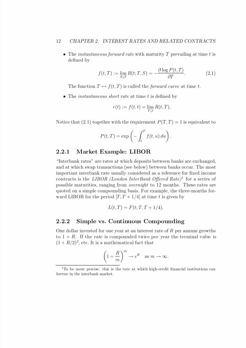
dollars at S with certainty.We are led to the following definitions.
• The simple (simply-compounded) forward rate for [T, S ] prevailing at tis given by
1+(S
−T )F (t; T, S ) :=
P (t, T )
P (t, S ) ⇔F (t; T, S ) =
1
S − T P (t, T )
P (t, S ) −1 .
• The simple spot rate for [t, T ] is
F (t, T ) := F (t; t, T ) =1
T − t
1
P (t, T )− 1
.
• The continuously compounded forward rate for [T, S ] prevailing at t isgiven by
eR(t;T,S )(S −T ) :=P (t, T )
P (t, S ) ⇔R(t; T, S ) =
−log P (t, S ) − log P (t, T )
S − T .
• The continuously compounded spot rate for [T, S ] is
R(t, T ) := R(t; t, T ) = − log P (t, T )
T − t.
8/7/2019 Fixed Income Models
http://slidepdf.com/reader/full/fixed-income-models 12/167

8/7/2019 Fixed Income Models
http://slidepdf.com/reader/full/fixed-income-models 13/167
2.2. INTEREST RATES 13
Moreover,
eR
= 1 + R + o(R) for R small.Example: e0.04 = 1.04081.
Since the exponential function has nicer analytic properties than powerfunctions, we often consider continuously compounded interest rates. Thismakes the theory more tractable.
2.2.3 Forward vs. Future Rates
Can forward rates predict the future spot rates?Consider a deterministic world. If markets are efficient (i.e. no arbitrage
= no riskless, systematic profit) we have necessarily
P (t, S ) = P (t, T )P (T, S ), ∀t ≤ T ≤ S. (2.2)
Proof. Suppose that P (t, S ) > P (t, T )P (T, S ) for some t ≤ T ≤ S . Then wefollow the strategy:
• At t: sell one S -bond, and buy P (T, S ) T -bonds.
Net cost: −P (t, S ) + P (t, T )P (T, S ) < 0.
•At T : receive P (T, S ) dollars and buy one S -bond.
• At S : pay one dollar, receive one dollar.
(Where do we use the assumption of a deterministic world?)The net is a riskless gain of −P (t, S )+P (t, T )P (T, S ) (×1/P (t, S )). This
is a pure arbitrage opportunity, which contradicts the assumption.If P (t, S ) < P (t, T )P (T, S ) the same profit can be realized by changing
sign in the strategy.
Taking logarithm in (2.2) yields
S T
f (t, u) du = S T
f (T, u) du, ∀t ≤ T ≤ S.
This is equivalent to
f (t, S ) = f (T, S ) = r(S ), ∀t ≤ T ≤ S

8/7/2019 Fixed Income Models
http://slidepdf.com/reader/full/fixed-income-models 14/167
14 CHAPTER 2. INTEREST RATES AND RELATED CONTRACTS
(as time goes by we walk along the forward curve: the forward curve is
shifted). In this case, the forward rate with maturity S prevailing at timet ≤ S is exactly the future short rate at S .
The real world is not deterministic though. We will see that in generalthe forward rate f (t, T ) is the conditional expectation of the short rate r(T )under a particular probability measure (forward measure), depending on T .
Hence the forward rate is a biased estimator for the future short rate.Forecasts of future short rates by forward rates have little or no predictivepower.
2.3 Bank Account and Short RatesThe return of a one dollar investment today (t = 0) over the period [0, ∆t]is given by
1
P (0, ∆t)= exp
∆t
0
f (0, u) du
= 1 + r(0)∆t + o(∆t).
Instantaneous reinvestment in 2∆t-bonds yields
1
P (0, ∆t)
1
P (∆t, 2∆t)= (1 + r(0)∆t)(1 + r(∆t)∆t) + o(∆t)
at time 2∆t, etc. This strategy of “rolling over”2 just maturing bonds leadsin the limit to the bank account (money-market account) B(t). Hence B(t)is the asset which growths at time t instantaneously at short rate r(t)
B(t + ∆t) = B(t)(1 + r(t)∆t) + o(∆t).
For ∆t → 0 this converges to
dB(t) = r(t)B(t)dt
and with B(0) = 1 we obtain
B(t) = exp
t0
r(s) ds
.
2This limiting process is made rigorous in [4].

8/7/2019 Fixed Income Models
http://slidepdf.com/reader/full/fixed-income-models 15/167
2.4. COUPON BONDS, SWAPS AND YIELDS 15
B is a risk-free asset insofar as its future value at time t + ∆t is known (up
to order ∆t) at time t. In stochastic terms we speak of a predictable process.For the same reason we speak of r(t) as the risk-free rate of return over theinfinitesimal period [t, t + dt].
B is important for relating amounts of currencies available at differenttimes: in order to have one dollar in the bank account at time T we need tohave
B(t)
B(T )= exp
− T t
r(s) ds
dollars in the bank account at time t ≤ T . This discount factor is stochastic:
it is not known with certainty at time t. There is a close connection to thedeterministic (=known at time t) discount factor given by P (t, T ). Indeed,we will see that the latter is the conditional expectation of the former underthe risk neutral probability measure.
Proxies for the Short Rate
→ JW[11](Chapter 3.5)
The short rate r(t) is a key interest rate in all models and fundamentalto no-arbitrage pricing. But it cannot be directly observed.
The overnight interest rate is not usually considered to be a good proxyfor the short rate, because the motives and needs driving overnight borrowersare very different from those of borrowers who want money for a month ormore.
The overnight fed funds rate is nevertheless comparatively stable andperhaps a fair proxy, but empirical studies suggest that it has low correlationwith other spot rates.
The best available proxy is given by one- or three-month spot rates sincethey are very liquid.
2.4 Coupon Bonds, Swaps and Yields
In most bond markets, there is only a relatively small number of zero-couponbonds traded. Most bonds include coupons.

8/7/2019 Fixed Income Models
http://slidepdf.com/reader/full/fixed-income-models 16/167
16 CHAPTER 2. INTEREST RATES AND RELATED CONTRACTS
2.4.1 Fixed Coupon Bonds
A fixed coupon bond is a contract specified by
• a number of future dates T 1 < · · · < T n (the coupon dates)
(T n is the maturity of the bond),
• a sequence of (deterministic) coupons c1, . . . , cn,
• a nominal value N ,
such that the owner receives ci at time T i, for i = 1, . . . , n, and N at terminaltime T
n. The price p(t) at time t
≤T
1of this coupon bond is given by the
sum of discounted cashflows
p(t) =ni=1
P (t, T i)ci + P (t, T n)N.
Typically, it holds that T i+1−T i ≡ δ, and the coupons are given as a fixedpercentage of the nominal value: ci ≡ KδN , for some fixed interest rate K .The above formula reduces to
p(t) = Kδn
i=1
P (t, T i) + P (t, T n)N.
2.4.2 Floating Rate Notes
There are versions of coupon bonds for which the value of the coupon isnot fixed at the time the bond is issued, but rather reset for every couponperiod. Most often the resetting is determined by some market interest rate(e.g. LIBOR).
A floating rate note is specified by
•a number of future dates T 0 < T 1 <
· · ·< T n,
• a nominal value N .
The deterministic coupon payments for the fixed coupon bond are now re-placed by
ci = (T i − T i−1)F (T i−1, T i)N,

8/7/2019 Fixed Income Models
http://slidepdf.com/reader/full/fixed-income-models 17/167
2.4. COUPON BONDS, SWAPS AND YIELDS 17
where F (T i−1, T i) is the prevailing simple market interest rate, and we note
that F (T i−1, T i) is determined already at time T i−1 (this is why here we haveT 0 in addition to the coupon dates T 1, . . . , T n), but that the cash-flow ci isat time T i.
The value p(t) of this note at time t ≤ T 0 is obtained as follows. Withoutloss of generality we set N = 1. By definition of F (T i−1, T i) we then have
ci =1
P (T i−1, T i)− 1.
The time t value of −1 paid out at T i is −P (t, T i). The time t value of 1
P (T i−1,T i)paid out at T i is P (t, T i−1):
• At t: buy a T i−1-bond. Cost: P (t, T i−1).
• At T i−1: receive one dollar and buy 1/P (T i−1, T i) T i-bonds. Zero netinvestment.
• At T i: receive 1/P (T i−1, T i) dollars.
The time t value of ci therefore is
P (t, T i−1) − P (t, T i).
Summing up we obtain the (surprisingly easy) formula
p(t) = P (t, T n) +ni=1
(P (t, T i−1) − P (t, T i)) = P (t, T 0).
In particular, for t = T 0: p(T 0) = 1.
2.4.3 Interest Rate Swaps
An interest rate swap is a scheme where you exchange a payment streamat a fixed rate of interest for a payment stream at a floating rate (typically
LIBOR).There are many versions of interest rate swaps. A payer interest rate
swap settled in arrears is specified by
• a number of future dates T 0 < T 1 < · · · < T n with T i − T i−1 ≡ δ
(T n is the maturity of the swap),

8/7/2019 Fixed Income Models
http://slidepdf.com/reader/full/fixed-income-models 18/167
18 CHAPTER 2. INTEREST RATES AND RELATED CONTRACTS
• a fixed rate K ,
• a nominal value N .
Of course, the equidistance hypothesis is only for convenience of notationand can easily be relaxed. Cashflows take place only at the coupon datesT 1, . . . , T n. At T i, the holder of the contract
• pays fixed KδN ,
• and receives floating F (T i−1, T i)δN .
The net cashflow at T i is thus
(F (T i−1, T i) − K )δN,
and using the previous results we can compute the value at t ≤ T 0 of thiscashflow as
N (P (t, T i−1) − P (t, T i) − KδP (t, T i)). (2.3)
The total value Π p(t) of the swap at time t ≤ T 0 is thus
Π p(t) = N
P (t, T 0) − P (t, T n) − Kδ
n
i=1
P (t, T i)
.
A receiver interest rate swap settled in arrears is obtained by changingthe sign of the cashflows at times T 1, . . . , T n. Its value at time t ≤ T 0 is thus
Πr(t) = −Π p(t).
The remaining question is how the “fair” fixed rate K is determined. The forward swap rate Rswap(t) at time t ≤ T 0 is the fixed rate K above whichgives Π p(t) = Πr(t) = 0. Hence
Rswap(t) =
P (t, T 0)
−P (t, T n)
δni=1 P (t, T i) .
The following alternative representation of Rswap(t) is sometimes useful.Since P (t, T i−1) − P (t, T i) = F (t; T i−1, T i)δP (t, T i), we can rewrite (2.3) as
NδP (t, T i) (F (t; T i−1, T i) − K ) .
8/7/2019 Fixed Income Models
http://slidepdf.com/reader/full/fixed-income-models 19/167
2.4. COUPON BONDS, SWAPS AND YIELDS 19
Summing up yields
Π p(t) = Nδni=1
P (t, T i) (F (t; T i−1, T i) − K ) ,
and thus we can write the swap rate as weighted average of simple forwardrates
Rswap(t) =ni=1
wi(t)F (t; T i−1, T i),
with weights
wi(t) =P (t, T i)n j=1 P (t, T j)
.
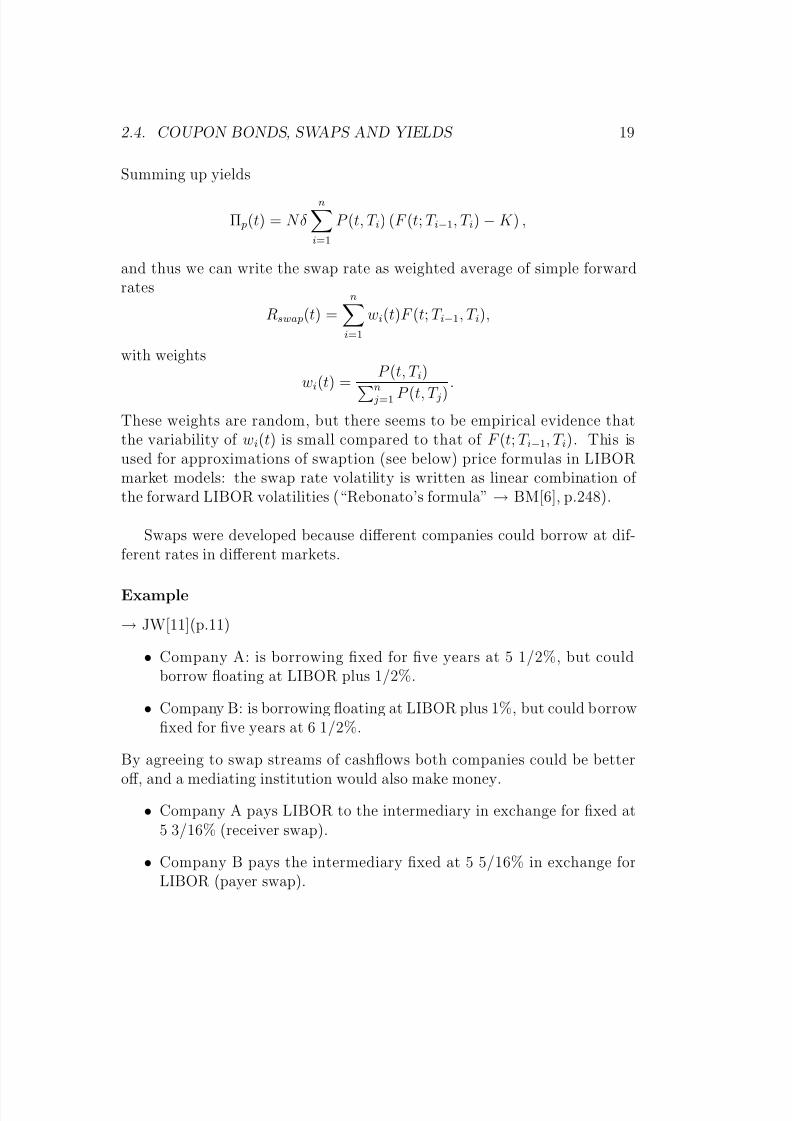
These weights are random, but there seems to be empirical evidence thatthe variability of wi(t) is small compared to that of F (t; T i−1, T i). This isused for approximations of swaption (see below) price formulas in LIBORmarket models: the swap rate volatility is written as linear combination of the forward LIBOR volatilities (“Rebonato’s formula” → BM[6], p.248).
Swaps were developed because different companies could borrow at dif-ferent rates in different markets.
Example
→ JW[11](p.11)
• Company A: is borrowing fixed for five years at 5 1/2%, but couldborrow floating at LIBOR plus 1/2%.
• Company B: is borrowing floating at LIBOR plus 1%, but could borrowfixed for five years at 6 1/2%.
By agreeing to swap streams of cashflows both companies could be better
off, and a mediating institution would also make money.• Company A pays LIBOR to the intermediary in exchange for fixed at
5 3/16% (receiver swap).
• Company B pays the intermediary fixed at 5 5/16% in exchange forLIBOR (payer swap).
8/7/2019 Fixed Income Models
http://slidepdf.com/reader/full/fixed-income-models 20/167
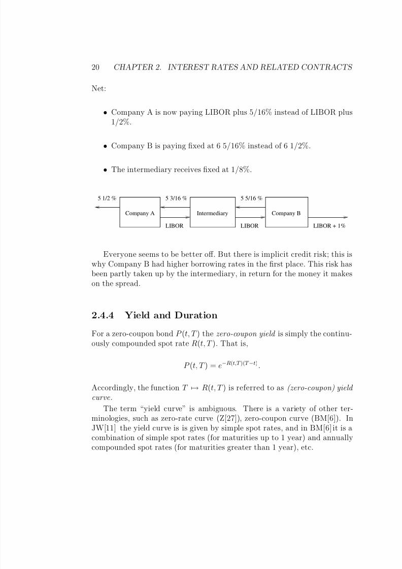
20 CHAPTER 2. INTEREST RATES AND RELATED CONTRACTS
Net:
• Company A is now paying LIBOR plus 5/16% instead of LIBOR plus1/2%.
• Company B is paying fixed at 6 5/16% instead of 6 1/2%.
• The intermediary receives fixed at 1/8%.
5 5/16 %5 3/16 %
LIBOR LIBOR LIBOR + 1%
5 1/2 %
Company A Intermediary Company B
Everyone seems to be better off. But there is implicit credit risk; this iswhy Company B had higher borrowing rates in the first place. This risk hasbeen partly taken up by the intermediary, in return for the money it makeson the spread.
2.4.4 Yield and Duration
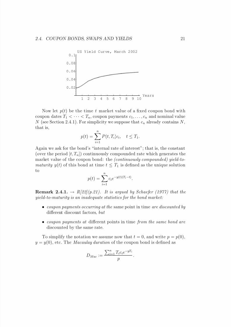
For a zero-coupon bond P (t, T ) the zero-coupon yield is simply the continu-ously compounded spot rate R(t, T ). That is,
P (t, T ) = e−R(t,T )(T −t).
Accordingly, the function T → R(t, T ) is referred to as (zero-coupon) yield
curve.The term “yield curve” is ambiguous. There is a variety of other ter-
minologies, such as zero-rate curve (Z[27]), zero-coupon curve (BM[6]). InJW[11] the yield curve is is given by simple spot rates, and in BM[6] it is acombination of simple spot rates (for maturities up to 1 year) and annuallycompounded spot rates (for maturities greater than 1 year), etc.
8/7/2019 Fixed Income Models
http://slidepdf.com/reader/full/fixed-income-models 21/167
2.4. COUPON BONDS, SWAPS AND YIELDS 21
1 2 3 4 5 6 7 8 9 10Years
0.02
0.04
0.06
0.08
0.1US Yield Curve, March 2002
Now let p(t) be the time t market value of a fixed coupon bond with
coupon dates T 1 < · · · < T n, coupon payments c1, . . . , cn and nominal valueN (see Section 2.4.1). For simplicity we suppose that cn already contains N ,that is,
p(t) =ni=1
P (t, T i)ci, t ≤ T 1.
Again we ask for the bond’s “internal rate of interest”; that is, the constant(over the period [t, T n]) continuously compounded rate which generates themarket value of the coupon bond: the (continuously compounded) yield-to-maturity y(t) of this bond at time t ≤ T 1 is defined as the unique solution
to p(t) =
ni=1
cie−y(t)(T i−t).
Remark 2.4.1. → R[22](p.21). It is argued by Schaefer (1977) that theyield-to-maturity is an inadequate statistics for the bond market:
• coupon payments occurring at the same point in time are discounted by different discount factors, but
• coupon payments at different points in time from the same bond are
discounted by the same rate.To simplify the notation we assume now that t = 0, and write p = p(0),
y = y(0), etc. The Macaulay duration of the coupon bond is defined as
DMac :=
ni=1 T icie
−yT i
p.
8/7/2019 Fixed Income Models
http://slidepdf.com/reader/full/fixed-income-models 22/167
8/7/2019 Fixed Income Models
http://slidepdf.com/reader/full/fixed-income-models 23/167
2.5. MARKET CONVENTIONS 23
• Actual/365: a year has 365 days, and the day-count convention for
T − t is given by
actual number of days between t and T
365.
• Actual/360: as above but the year counts 360 days.
• 30/360: months count 30 and years 360 days. Let t = (d1, m1, y1) andT = (d2, m2, y2). The day-count convention for T − t is given by
min(d2, 30) + (30
−d1)+
360+
(m2
−m1
−1)+
12+ y
2 −y
1.
Example: The time between t=January 4, 2000 and T =July 4, 2002 isgiven by
4 + (30 − 4)
360+
7 − 1 − 1
12+ 2002 − 2000 = 2.5.
When extracting information on interest rates from data, it is importantto realize for which day-count convention a specific interest rate is quoted.
→BM[6](p.4), Z[27](Sect. 5.1)
2.5.2 Coupon Bonds
→ MR[19](Sect. 11.2), Z[27](Sect. 5.2), J[13](Chapter 2)Coupon bonds issued in the American (European) markets typically have
semi-annual (annual) coupon payments.Debt securities issued by the U.S. Treasury are divided into three classes:
• Bills: zero-coupon bonds with time to maturity less than one year.
• Notes: coupon bonds (semi-annual) with time to maturity between 2and 10 years.
• Bonds: coupon bonds (semi-annual) with time to maturity between 10and 30 years3.
3Recently, the issuance of 30 year treasury bonds has been stopped.

8/7/2019 Fixed Income Models
http://slidepdf.com/reader/full/fixed-income-models 24/167
24 CHAPTER 2. INTEREST RATES AND RELATED CONTRACTS
In addition to bills, notes and bonds, Treasury securities called STRIPS
(separate trading of registered interest and principal of securities) have tradedsince August 1985. These are the coupons or principal (=nominal) amountsof Treasury bonds trading separately through the Federal Reserve’s book-entry system. They are synthetically created zero-coupon bonds of longermaturities than a year. They were created in response to investor demands.
2.5.3 Accrued Interest, Clean Price and Dirty Price
Remember that we had for the price of a coupon bond with coupon datesT 1, . . . , T n and payments c1, . . . , cn the price formula
p(t) =ni=1
ciP (t, T i), t ≤ T 1.
For t ∈ (T 1, T 2] we have
p(t) =ni=2
ciP (t, T i),
etc. Hence there are systematic discontinuities of the price trajectory at
t = T 1, . . . , T n which is due to the coupon payments. This is why prices aredifferently quoted at the exchange.
The accrued interest at time t ∈ (T i−1, T i] is defined by
AI (i; t) := cit − T i−1
T i − T i−1
(where now time differences are taken according to the day-count conven-tion). The quoted price, or clean price, of the coupon bond at time t is
pclean(t) := p(t) − AI (i; t), t ∈ (T i−1, T i].
That is, whenever we buy a coupon bond quoted at a clean price of pclean(t)at time t ∈ (T i−1, T i], the cash price, or dirty price, we have to pay is
p(t) = pclean(t) + AI (i; t).
8/7/2019 Fixed Income Models
http://slidepdf.com/reader/full/fixed-income-models 25/167
2.6. CAPS AND FLOORS 25
2.5.4 Yield-to-Maturity
The quoted (annual) yield-to-maturity y(t) on a Treasury bond at time t = T iis defined by the relationship
pclean(T i) =n
j=i+1
rcN/2
(1 + y(T i)/2) j−i+
N
(1 + y(T i)/2)n−i,
and at t ∈ [T i, T i+1)
pclean(t) =n
j=i+1
rcN/2
(1 + y(t)/2) j−i−1+τ +
N
(1 + y(t)/2)n−i−1+τ ,
where rc is the (annualized) coupon rate, N the nominal amount and
τ =T i+1 − t
T i+1 − T i
is again given by the day-count convention, and we assume here that
T i+1 − T i ≡ 1/2 (semi-annual coupons).
2.6 Caps and Floors→ BM[6](Sect. 1.6), Z[27](Sect. 5.6.2)
Caps
A caplet with reset date T and settlement date T + δ pays the holder thedifference between a simple market rate F (T, T + δ) (e.g. LIBOR) and thestrike rate κ. Its cashflow at time T + δ is
δ(F (T, T + δ) − κ)+.
A cap is a strip of caplets. It thus consists of
• a number of future dates T 0 < T 1 < · · · < T n with T i − T i−1 ≡ δ
(T n is the maturity of the cap),
• a cap rate κ.

8/7/2019 Fixed Income Models
http://slidepdf.com/reader/full/fixed-income-models 26/167
26 CHAPTER 2. INTEREST RATES AND RELATED CONTRACTS
Cashflows take place at the dates T 1, . . . , T n. At T i the holder of the cap
receivesδ(F (T i−1, T i) − κ)+. (2.4)
Let t ≤ T 0. We write
Cpl(i; t), i = 1, . . . , n ,
for the time t price of the ith caplet with reset date T i−1 and settlement dateT i, and
Cp(t) =ni=1
Cpl(i; t)
for the time t price of the cap.A cap gives the holder a protection against rising interest rates. It guar-
antees that the interest to be paid on a floating rate loan never exceeds thepredetermined cap rate κ.
It can be shown (→ exercise) that the cashflow (2.4) at time T i is theequivalent to (1 + δκ) times the cashflow at date T i−1 of a put option on aT i-bond with strike price 1/(1 + δκ) and maturity T i−1, that is,
(1 + δκ)
1
1 + δκ− P (T i−1, T i)
+
.
This is an important fact because many interest rate models have explicitformulae for bond option values, which means that caps can be priced veryeasily in those models.
Floors
A floor is the converse to a cap. It protects against low rates. A floor is astrip of floorlets , the cashflow of which is – with the same notation as above– at time T i
δ(κ − F (T i−1, T i))+.
Write F ll(i; t) for the price of the ith floorlet and
F l(t) =ni=1
F ll(i; t)
for the price of the floor.
8/7/2019 Fixed Income Models
http://slidepdf.com/reader/full/fixed-income-models 27/167
2.6. CAPS AND FLOORS 27
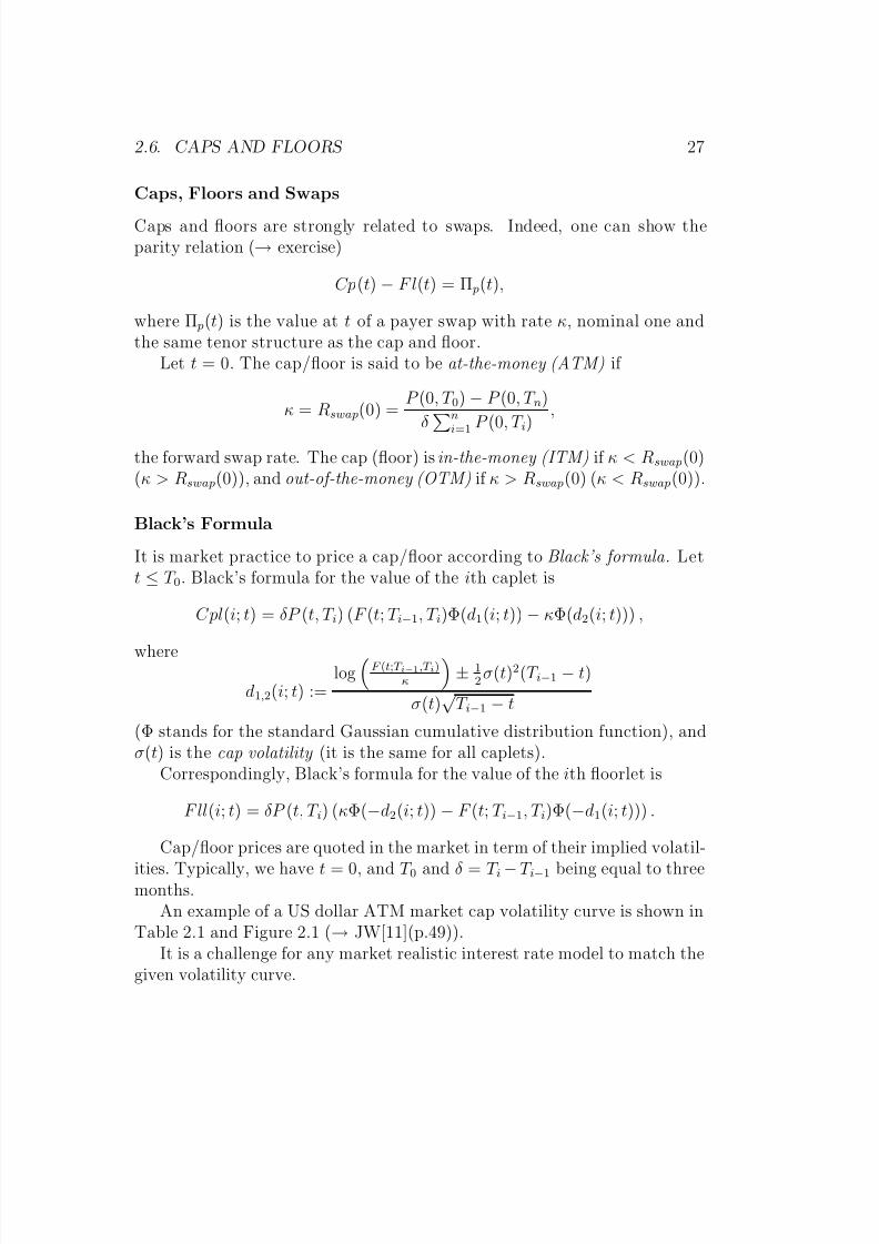
Caps, Floors and Swaps
Caps and floors are strongly related to swaps. Indeed, one can show theparity relation (→ exercise)
Cp(t) − F l(t) = Π p(t),
where Π p(t) is the value at t of a payer swap with rate κ, nominal one andthe same tenor structure as the cap and floor.
Let t = 0. The cap/floor is said to be at-the-money (ATM) if
κ = Rswap(0) =P (0, T 0) − P (0, T n)
δni=1 P (0, T i)
,
the forward swap rate. The cap (floor) is in-the-money (ITM) if κ < Rswap(0)(κ > Rswap(0)), and out-of-the-money (OTM) if κ > Rswap(0) (κ < Rswap(0)).
Black’s Formula
It is market practice to price a cap/floor according to Black’s formula . Lett ≤ T 0. Black’s formula for the value of the ith caplet is
Cpl(i; t) = δP (t, T i) (F (t; T i−1, T i)Φ(d1(i; t)) − κΦ(d2(i; t))) ,
where
d1,2(i; t) :=logF (t;T i−1,T i)
κ
± 1
2σ(t)2(T i−1 − t)
σ(t)√
T i−1 − t
(Φ stands for the standard Gaussian cumulative distribution function), andσ(t) is the cap volatility (it is the same for all caplets).
Correspondingly, Black’s formula for the value of the ith floorlet is
F ll(i; t) = δP (t, T i) (κΦ(−d2(i; t)) − F (t; T i−1, T i)Φ(−d1(i; t))) .
Cap/floor prices are quoted in the market in term of their implied volatil-
ities. Typically, we have t = 0, and T 0 and δ = T i− T i−1 being equal to threemonths.
An example of a US dollar ATM market cap volatility curve is shown inTable 2.1 and Figure 2.1 (→ JW[11](p.49)).
It is a challenge for any market realistic interest rate model to match thegiven volatility curve.

8/7/2019 Fixed Income Models
http://slidepdf.com/reader/full/fixed-income-models 28/167
28 CHAPTER 2. INTEREST RATES AND RELATED CONTRACTS
Table 2.1: US dollar ATM cap volatilities, 23 July 1999
Maturity ATM vols(in years) (in %)
1 14.12 17.43 18.54 18.85 18.96 18.77 18.48 18.2
10 17.712 17.015 16.520 14.730 12.4
Figure 2.1: US dollar ATM cap volatilities, 23 July 1999
5 10 15 20 25 30
12%
14%
16%
18%

8/7/2019 Fixed Income Models
http://slidepdf.com/reader/full/fixed-income-models 29/167
2.7. SWAPTIONS 29
2.7 Swaptions
A European payer (receiver) swaption with strike rate K is an option givingthe right to enter a payer (receiver) swap with fixed rate K at a given futuredate, the swaption maturity . Usually, the swaption maturity coincides withthe first reset date of the underlying swap. The underlying swap lenghtT n − T 0 is called the tenor of the swaption.
Recall that the value of a payer swap with fixed rate K at its first resetdate, T 0, is
Π p(T 0, K ) = N n
i=1
P (T 0, T i)δ(F (T 0; T i−1, T i) − K ).
Hence the payoff of the swaption with strike rate K at maturity T 0 is
N
ni=1
P (T 0, T i)δ(F (T 0; T i−1, T i) − K )
+
. (2.5)
Notice that, contrary to the cap case, this payoff cannot be decomposedinto more elementary payoffs. This is a fundamental difference betweencaps/floors and swaptions. Here the correlation between different forwardrates will enter the valuation procedure.
Since Π p(T 0, Rswap(T 0)) = 0, one can show (→ exercise) that the payoff (2.5) of the payer swaption at time T 0 can also be written as
Nδ(Rswap(T 0) − K )+ni=1
P (T 0, T i),
and for the receiver swaption
Nδ(K − Rswap(T 0))+ni=1
P (T 0, T i).
Accordingly, at time t ≤ T 0, the payer (receiver) swaption with strike rateK is said to be ATM , ITM , OTM , if
K = Rswap(t), K < (>)Rswap(t), K > (<)Rswap(t),
respectively.
8/7/2019 Fixed Income Models
http://slidepdf.com/reader/full/fixed-income-models 30/167
30 CHAPTER 2. INTEREST RATES AND RELATED CONTRACTS
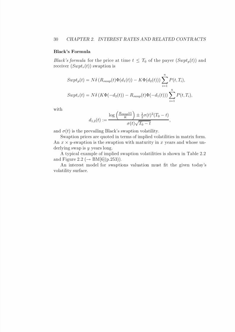
Black’s Formula
Black’s formula for the price at time t ≤ T 0 of the payer (Swpt p(t)) andreceiver (Swptr(t)) swaption is
Swpt p(t) = Nδ (Rswap(t)Φ(d1(t)) − K Φ(d2(t)))ni=1
P (t, T i),
Swptr(t) = Nδ (K Φ(−d2(t)) − Rswap(t)Φ(−d1(t)))ni=1
P (t, T i),
with
d1,2(t) := log Rswap(t)
K ±1
2 σ(t)2
(T 0 − t)σ(t)
√T 0 − t
,
and σ(t) is the prevailing Black’s swaption volatility.Swaption prices are quoted in terms of implied volatilities in matrix form.
An x × y-swaption is the swaption with maturity in x years and whose un-derlying swap is y years long.
A typical example of implied swaption volatilities is shown in Table 2.2and Figure 2.2 (→ BM[6](p.253)).
An interest model for swaptions valuation must fit the given today’svolatility surface.

8/7/2019 Fixed Income Models
http://slidepdf.com/reader/full/fixed-income-models 31/167
2.7. SWAPTIONS 31
Table 2.2: Black’s implied volatilities (in %) of ATM swaptions on May 16,2000. Maturities are 1,2,3,4,5,7,10 years, swaps lengths from 1 to 10 years.
1y 2y 3y 4y 5y 6y 7y 8y 9y 10y1y 16.4 15.8 14.6 13.8 13.3 12.9 12.6 12.3 12.0 11.72y 17.7 15.6 14.1 13.1 12.7 12.4 12.2 11.9 11.7 11.43y 17.6 15.5 13.9 12.7 12.3 12.1 11.9 11.7 11.5 11.34y 16.9 14.6 12.9 11.9 11.6 11.4 11.3 11.1 11.0 10.85y 15.8 13.9 12.4 11.5 11.1 10.9 10.8 10.7 10.5 10.4
7y 14.5 12.9 11.6 10.8 10.4 10.3 10.1 9.9 9.8 9.610y 13.5 11.5 10.4 9.8 9.4 9.3 9.1 8.8 8.6 8.4
Figure 2.2: Black’s implied volatilities (in %) of ATM swaptions on May 16,
2000.
2 4 68
10
Maturity
24 6 8
10
Tenor
10
12
14
16
Vol

8/7/2019 Fixed Income Models
http://slidepdf.com/reader/full/fixed-income-models 32/167
32 CHAPTER 2. INTEREST RATES AND RELATED CONTRACTS
8/7/2019 Fixed Income Models
http://slidepdf.com/reader/full/fixed-income-models 33/167
Chapter 3
Some Statistics of the Yield
Curve
3.1 Principal Component Analysis (PCA)
→ JW[11](Chapter 16.2), [21]
• Let x(1), . . . , x(N ) be a sample of a random n × 1 vector x.
• Form the empirical n × n covariance matrix Σ,
Σij =
N k=1(xi(k) − µ[xi])(x j(k) − µ[x j ])
N − 1
=
N k=1 xi(k)xi(k) − Nµ[xi]µ[x j]
N − 1,
where
µ[xi] :=1
N
N k=1
xi(k) (mean of xi).
We assume that Σ is non-degenerate (otherwise we can express an xias linear combination of the other x js).
• There exists a unique orthogonal matrix A = ( p1, . . . , pn) (that is,A−1 = AT and Aij = p j;i) consisting of orthonormal n × 1 Eigenvectors
pi of Σ such thatΣ = ALAT ,
33

8/7/2019 Fixed Income Models
http://slidepdf.com/reader/full/fixed-income-models 34/167
34 CHAPTER 3. STATISTICS OF THE YIELD CURVE
where L = diag(λ1, . . . , λn) with λ1 ≥ · · · ≥ λn > 0 (the Eigenvalues
of Σ).
• Define z := AT x. Then
Cov[zi, z j ] =n
k,l=1
AT ikCov[xk, xl]AT jl =
AT ΣA
ij
= λiδij.
Hence the zis are uncorrelated.
• The principal components (PCs) are the n × 1 vectors p1, . . . , pn:
x = Az = z1 p1 + · · · zn pn.
The importance of component pi is determined by the size of the cor-responding Eigenvalue, λi, which indicates the amount of variance ex-plained by pi. The key statistics is the proportion
λin j=1 λ j
,
the explained variance by pi.
• Normalization: let w := (L1/2)−1z, where L1/2 := diag(√
λ1, . . . ,√
λn),and w = w − µ[w] (µ[w]=mean of w). Then
µ[w] = 0, Cov[wi, w j] = Cov[ wi, w j] = δij ,
and
x = µ[x] + AL1/2w = µ[x] +n j=1
p j
λ jw j.
In components
xi = µ[xi] +n j=1
Aij
λ jw j .
•Sometimes the following view is useful (
→R[22](Chapter 3)): set
σi := V ar[xi]1/2 =
Σii
1/2
=
n j=1
A2ijλ j
1/2
vi :=xi − µ[xi]
σi=
n j=1 Aij
λ jw j
σi, i = 1, . . . , n .
8/7/2019 Fixed Income Models
http://slidepdf.com/reader/full/fixed-income-models 35/167
3.2. PCA OF THE YIELD CURVE 35
Then we have µ[vi] = 0, µ[v2i ] = 1 and
xi = µ[xi] + σivi.
It can be appropriate to assume a parametric functional form (→ re-duction of parameters) of the correlation structure of x,
Corr[xi, x j] = Cov[vi, v j ] =Σij
σiσ j=
nk=1 AikA jkλk
σiσ j= ρ(π; i, j),
where π is some low-dimensional parameter (this is adapted to thecalibration of market models → BM[6](Chapter 6.9)).
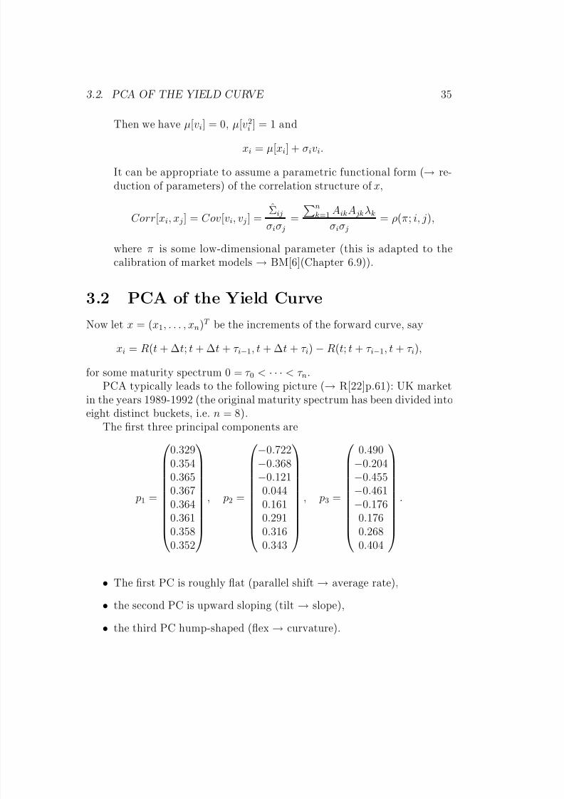
3.2 PCA of the Yield Curve
Now let x = (x1, . . . , xn)T be the increments of the forward curve, say
xi = R(t + ∆t; t + ∆t + τ i−1, t + ∆t + τ i) − R(t; t + τ i−1, t + τ i),
for some maturity spectrum 0 = τ 0 < · · · < τ n.PCA typically leads to the following picture (→ R[22]p.61): UK market
in the years 1989-1992 (the original maturity spectrum has been divided intoeight distinct buckets, i.e. n = 8).
The first three principal components are
p1 =
0.3290.3540.3650.3670.3640.3610.3580.352
, p2 =
−0.722−0.368−0.1210.0440.1610.2910.3160.343
, p3 =
0.490−0.204−0.455−0.461−0.1760.1760.2680.404
.
• The first PC is roughly flat (parallel shift → average rate),
• the second PC is upward sloping (tilt → slope),
• the third PC hump-shaped (flex → curvature).

8/7/2019 Fixed Income Models
http://slidepdf.com/reader/full/fixed-income-models 36/167
36 CHAPTER 3. STATISTICS OF THE YIELD CURVE
Figure 3.1: First Three PCs.
2 3 4 5 6 7 8
-0.8
-0.6
-0.4
-0.2
0.2
0.4
0.6
Table 3.1: Explained Variance of the Principal Components (PCs).
PC ExplainedVariance (%)
1 92.172 6.933 0.61
4 0.245 0.036–8 0.01
The first three PCs explain more than 99 % of the variance of x (→ Table 3.1).
PCA of the yield curve goes back to the seminal paper by Littermanand Scheinkman (91) [17] (Prof. J. Scheinkman is at the Department of Economics, Princeton University).
3.3 Correlation
→ R[22](p.58)A typical example of correlation among forward rates is provided by

8/7/2019 Fixed Income Models
http://slidepdf.com/reader/full/fixed-income-models 37/167
3.3. CORRELATION 37
Brown and Schaefer (1994). The data is from the US Treasury yield curve
1987–1994. The following matrix (→ Figure 3.2)
1 0.87 0.74 0.69 0.64 0.61 0.96 0.93 0.9 0.85
1 0.99 0.95 0.921 0.97 0.93
1 0.951
shows the correlation for changes of forward rates of maturities
0, 0.5, 1, 1.5, 2, 3 years.
Figure 3.2: Correlation between the short rate and instantaneous forwardrates for the US Treasury curve 1987–1994
0.5 1 1.5 2 2.5 3
0.6
0.7
0.8
0.9
1
→Decorrelation occurs quickly.
→ Exponentially decaying correlation structure is plausible.

8/7/2019 Fixed Income Models
http://slidepdf.com/reader/full/fixed-income-models 38/167
38 CHAPTER 3. STATISTICS OF THE YIELD CURVE

8/7/2019 Fixed Income Models
http://slidepdf.com/reader/full/fixed-income-models 39/167
Chapter 4
Estimating the Yield Curve
4.1 A Bootstrapping Example
→ JW[11](p.129–136)This is a naive bootstrapping method of fitting to a money market yield
curve. The idea is to build up the yield curve
from shorter maturities to longer maturities.
We take Yen data from 9 January, 1996 (→ JW[11](Section 5.4)). The
spot date t0 is 11 January, 1996. The day-count convention is Actual/360,
δ(T, S ) =actual number of days between T and S
360.
Table 4.1: Yen data, 9 January 1996.
LIBOR (%) Futures Swaps (%)o/n 0.49 20 Mar 96 99.34 2y 1.141w 0.50 19 Jun 96 99.25 3y 1.60
1m 0.53 18 Sep 96 99.10 4y 2.042m 0.55 18 Dec 96 98.90 5y 2.433m 0.56 7y 3.01
10y 3.36
39

8/7/2019 Fixed Income Models
http://slidepdf.com/reader/full/fixed-income-models 40/167

8/7/2019 Fixed Income Models
http://slidepdf.com/reader/full/fixed-income-models 41/167
4.1. A BOOTSTRAPPING EXAMPLE 41
• Yen swaps have semi-annual cashflows at dates
U 1, . . . , U 20 =
11/7/96, 13/1/97,11/7/97, 12/1/98,13/7/98, 11/1/99,12/7/99, 11/1/00,11/7/00, 11/1/01,11/7/01, 11/1/02,11/7/02, 13/1/03,11/7/03, 12/1/04,12/7/04, 11/1, 05,11/7/05, 11/1/06
.
For a swap with maturity U n the swap rate at t0 is given by
Rswap(t0, U n) =1 − P (t0, U n)n
i=1 δ(U i−1, U i) P (t0, U i), (U 0 := t0).
From the data we have Rswap(t0, U i) for i = 4, 6, 8, 10, 14, 20.
We obtain P (t0, U 1), P (t0, U 2) (and hence Rswap(t0, U 1), Rswap(t0, U 2))by linear interpolation of the continuously compounded spot rates
R(t0, U 1) = 6991
R(t0, T 2) + 2291
R(t0, T 3)
R(t0, U 2) =65
91R(t0, T 4) +
26
91R(t0, T 5).
All remaining swap rates are obtained by linear interpolation. Formaturity U 3 this is
Rswap(t0, U 3) =1
2(Rswap(t0, U 2) + Rswap(t0, U 4)).
We have (→ exercise)
P (t0, U n) =1 − Rswap(t0, U n)
n−1i=1 δ(U i−1, U i) P (t0, U i)
1 + Rswap(t0, U n)δ(U n−1, U n).
This gives P (t0, U n) for n = 3, . . . , 20.

8/7/2019 Fixed Income Models
http://slidepdf.com/reader/full/fixed-income-models 42/167
42 CHAPTER 4. ESTIMATING THE YIELD CURVE
Figure 4.1: Zero-coupon bond curve
2 4 6 8 10
Time to maturity
0.2
0.4
0.6
0.8
1
In Figure 4.1 is the implied zero-coupon bond price curve
P (t0, ti), i = 0, . . . , 29
(we have 29 points and set P (t0, t0) = 1).The spot and forward rate curves are in Figure 4.2. Spot and forward
rates are continuously compounded
R(t0, ti) = − log P (t0, ti)δ(t0, ti)
R(t0, ti, ti+1) = − log P (t0, ti+1) − log P (t0, ti)
δ(ti, ti+1), i = 1, . . . , 29.
The forward curve, reflecting the derivative of T → − log P (t0, T ), is veryunsmooth and sensitive to slight variations (errors) in prices.
Figure 4.3 shows the spot rate curves from LIBOR, futures and swaps. Itis evident that the three curves are not coincident to a common underlyingcurve. Our naive method made no attempt to meld the three curves together.
→ The entire yield curve is constructed from relatively few instruments. Themethod exactly reconstructs market prices (this is desirable for interestrate option traders). But it produces an unstable, non-smooth forwardcurve.

8/7/2019 Fixed Income Models
http://slidepdf.com/reader/full/fixed-income-models 43/167
4.1. A BOOTSTRAPPING EXAMPLE 43
Figure 4.2: Spot rates (lower curve), forward rates (upper curve)
2 4 6 8 10
Time to maturity
0.01
0.02
0.03
0.04
0.05
0.06
Figure 4.3: Comparison of money market curves
0.5 1 1.5 2
Time to maturity
0.005
0.0060.007
0.008
0.009
0.01
0.011
0.012
→ Another method would be to estimate a smooth yield curve parametri-cally from the market rates (for fund managers, long term strategies).
The main difficulties with our method are:
• Futures rates are treated as forward rates. In reality futures rates aregreater than forward rates. The amount by which the futures rate isabove the forward rate is called the convexity adjustment, which is

8/7/2019 Fixed Income Models
http://slidepdf.com/reader/full/fixed-income-models 44/167
44 CHAPTER 4. ESTIMATING THE YIELD CURVE
model dependend. An example is
forward rate = futures rate − 1
2σ2τ 2,
where τ is the time to maturity of the futures contract, and σ is thevolatility parameter.
• LIBOR rates beyond the “stup date” T 1 = 20/3/96 (that is, at S 5 =11/4/96) are ignored once P (t0, T 1) is found. In general, the segmentsof LIBOR, futures and swap markets overlap.
• Swap rates are inappropriately interpolated. The linear interpolation
produces a “sawtooth” in the forward rate curve. However, in somemarkets intermediate swaps are indeed priced as if their prices werefound by linear interpolation.
4.2 General Case
The general problem of finding today’s (t0) term structure of zero-couponbond prices (or the discount function )
x → D(x) := P (t0, t0 + x)
can be formulated as p = C · d + ,
where p is a vector of n market prices, C the related cashflow matrix, andd = (D(x1), . . . , D(xN )) with cashflow dates t0 < T 1 < · · · < T N ,
T i − t0 = xi,
and a vector of pricing errors. Reasons for including errors are
• prices are never exactly simultaneous,
• round-off errors in the quotes (bid-ask spreads, etc),
• liquidity effects,
• tax effects (high coupons, low coupons),
• allows for smoothing.
8/7/2019 Fixed Income Models
http://slidepdf.com/reader/full/fixed-income-models 45/167
4.2. GENERAL CASE 45
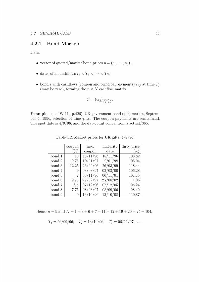
4.2.1 Bond Markets
Data:
• vector of quoted/market bond prices p = ( p1, . . . , pn),
• dates of all cashflows t0 < T 1 < · · · < T N ,
• bond i with cashflows (coupon and principal payments) ci,j at time T j(may be zero), forming the n × N cashflow matrix
C = (ci,j) 1≤i≤n1≤j≤N
.
Example (→ JW[11], p.426): UK government bond (gilt) market, Septem-ber 4, 1996, selection of nine gilts. The coupon payments are semiannual.The spot date is 4/9/96, and the day-count convention is actual/365.
Table 4.2: Market prices for UK gilts, 4/9/96.
coupon next maturity dirty price(%) coupon date ( pi)bond 1 10 15/11/96 15/11/96 103.82bond 2 9.75 1 9/01/97 1 9/01/98 106.04bond 3 12.25 26/09/96 26/03/99 118.44bond 4 9 03/03/97 03/03/00 106.28bond 5 7 06/11/96 06/11/01 101.15bond 6 9.75 2 7/02/97 2 7/08/02 111.06bond 7 8.5 07/12/96 07/12/05 106.24bond 8 7.75 08/03/97 08/09/06 98.49bond 9 9 13/10/96 13/10/08 110.87
Hence n = 9 and N = 1 + 3 + 6 + 7 + 11 + 12 + 19 + 20 + 25 = 104,
T 1 = 26/09/96, T 2 = 13/10/96, T 3 = 06/11/97, . . . .

8/7/2019 Fixed Income Models
http://slidepdf.com/reader/full/fixed-income-models 46/167
46 CHAPTER 4. ESTIMATING THE YIELD CURVE
No bonds have cashflows at the same date. The 9 × 10⁴ cashflow matrix is
C =
0 0 0 105 0 0 0 0 0 0 . . .0 0 0 0 0 4.875 0 0 0 0 . . .
6.125 0 0 0 0 0 0 0 0 6.125 . . .0 0 0 0 0 0 0 4.5 0 0 . . .0 0 3.5 0 0 0 0 0 0 0 . . .0 0 0 0 0 0 4.875 0 0 0 . . .0 0 0 0 4.25 0 0 0 0 0 . . .0 0 0 0 0 0 0 0 3.875 0 . . .0 4.5 0 0 0 0 0 0 0 0 . . .
4.2.2 Money Markets
Money market data can be put into the same price–cashflow form as above.
LIBOR (rate L, maturity T ): p = 1 and c = 1 + (T − t0)L at T .
FRA (forward rate F for [T, S ]): p = 0, c1 = −1 at T 1 = T , c2 = 1+(S −T )F at T 2 = S .
Swap (receiver, swap rate K , tenor t0 ≤ T 0 < · · · < T n, T i − T i−1 ≡ δ):
since
0 = −D(T 0 − t0) + δK n j=1
D(T j − t0) + (1 + δK )D(T n − t0),
• if T 0 = t0: p = 1, c1 = · · · = cn−1 = δK , cn = 1 + δK ,
• if T 0 > t0: p = 0, c0 = −1, c1 = · · · = cn−1 = δK , cn = 1 + δK .
→ at t0: LIBOR and swaps have notional price 1, FRAs and forward swapshave notional price 0.
Example (→ JW[11], p.428): US money market on October 6, 1997.The day-count convention is Actual/360. The spot date t0 is 8/10/97.
LIBOR is for o/n (1/365), 1m (33/360), and 3m (92/360).

8/7/2019 Fixed Income Models
http://slidepdf.com/reader/full/fixed-income-models 47/167

8/7/2019 Fixed Income Models
http://slidepdf.com/reader/full/fixed-income-models 48/167
48 CHAPTER 4. ESTIMATING THE YIELD CURVE
the 19 × 47 cashflow matrix C are
c11 0 0 0 0 0 0 0 0 0 0 0 0 00 0 c23 0 0 0 0 0 0 0 0 0 0 00 0 0 0 0 c36 0 0 0 0 0 0 0 00 −1 0 0 0 0 c47 0 0 0 0 0 0 00 0 0 −1 0 0 0 c58 0 0 0 0 0 00 0 0 0 −1 0 0 0 c69 0 0 0 0 00 0 0 0 0 0 0 0 −1 c7,10 0 0 0 00 0 0 0 0 0 0 0 0 −1 c8,11 0 0 00 0 0 0 0 0 0 0 0 0 −1 0 c9,13 00 0 0 0 0 0 0 0 0 0 0 0
−1 c10,14
0 0 0 0 0 0 0 0 0 0 0 c11,12 0 00 0 0 0 0 0 0 0 0 0 0 c12,12 0 00 0 0 0 0 0 0 0 0 0 0 c13,12 0 00 0 0 0 0 0 0 0 0 0 0 c14,12 0 00 0 0 0 0 0 0 0 0 0 0 c15,12 0 00 0 0 0 0 0 0 0 0 0 0 c16,12 0 00 0 0 0 0 0 0 0 0 0 0 c17,12 0 00 0 0 0 0 0 0 0 0 0 0 c18,12 0 00 0 0 0 0 0 0 0 0 0 0 c19,12 0 0
with
c11 = 1.00016, c23 = 1.00516, c36 = 1.01461,c47 = 1.01448, c58 = 1.01451, c69 = 1.01456, c7,10 = 1.01459,
c8,11 = 1.01471, c9,13 = 1.01486, c10,14 = 1.01517c11,12 = 0.060125, c12,12 = 0.061082, c13,12 = 0.0616,
c14,12 = 0.0622, c15,12 = 0.0632, c16,12 = 0.0642,
c17,12 = c18,12 = c19,12 = 0.0656.
4.2.3 Problems
Typically, we have n N . Moreover, many entries of C are zero (differentcashflow dates). This makes ordinary least square (OLS) regression
mind∈RN
2 | = p − C · d (⇒ C T p = C T Cd∗)
unfeasible.

8/7/2019 Fixed Income Models
http://slidepdf.com/reader/full/fixed-income-models 49/167
4.2. GENERAL CASE 49
One could chose the data set such that cashflows are at same points in
time (say four dates each year) and the cashflow matrix C is not entirely fullof zeros (Carleton–Cooper (1976)). Still regression only yields values D(xi)at the payment dates t0 + xi
→ interpolation technics necessary.
But there is nothing to regularize the discount factors (discount factors of similar maturity can be very different). As a result this leads to a raggedspot rate (yield) curve, and even worse for forward rates.
4.2.4 Parametrized Curve FamiliesReduction of parameters and smooth yield curves can be achieved by usingparametrized families of smooth curves
D(x) = D(x; z) = exp
− x
0
φ(u; z) du
, z ∈ Z ,
with state space Z ⊂ Rm.For regularity reasons (see below) it is best to estimate the forward curve
R+ x → f (t0, t0 + x) = φ(x) = φ(x; z).
This leads to a nonlinear optimization problem
minz∈Z
p − C · d(z) ,
with
di(z) = exp
− xi
0
φ(u; z) du
for some payment tenor 0 < x1 < · · · < xN .
Linear Families
Fix a set of basis functions ψ1, . . . , ψm (preferably with compact support ),and let
φ(x; z) = z1ψ1(x) + · · · + zmψm(x).

8/7/2019 Fixed Income Models
http://slidepdf.com/reader/full/fixed-income-models 50/167
50 CHAPTER 4. ESTIMATING THE YIELD CURVE
Cubic B-splines A cubic spline is a piecewise cubic polynomial that is
everywhere twice differentiable. It interpolates values at m + 1 knot pointsξ0 < · · · < ξm. Its general form is
σ(x) =3i=0
aixi +
m−1 j=1
b j(x − ξ j)3+,
hence it has m + 3 parameters a0, . . . , a4, b1, . . . , bm−1 (a kth degree splinehas m + k parameters). The spline is uniquely characterized by specificationof σ or σ at ξ0 and ξm.
Introduce six extra knot points
ξ−3 < ξ−2 < ξ−1 < ξ0 < · · · < ξm < ξm+1 < ξm+2 < ξm+3.
A basis for the cubic splines on [ξ0, ξm] is given by the m + 3 B-splines
ψk(x) =k+4 j=k
k+4
i=k,i= j
1
ξi − ξ j
(x − ξ j)
3+, k = −3, . . . , m − 1.
The B-spline ψk is zero outside [ξk, ξk+4].
Figure 4.4: B-spline with knot points 0, 1, 6, 8, 11.
2 4 6 8 10 12
0.01
0.02
0.03
0.04
0.05
0.06

8/7/2019 Fixed Income Models
http://slidepdf.com/reader/full/fixed-income-models 51/167
4.2. GENERAL CASE 51
Estimating the Discount Function B-splines can also be used to esti-
mate the discount function directly (Steeley (1991)),
D(x; z) = z1ψ1(x) + · · · + zmψm(x).
With
d(z) =
D(x1; z)
...D(xN ; z)
=
ψ1(x1) · · · ψm(x1)
......
ψ1(xN ) · · · ψm(xN )
·
z1
...zm
=: Ψ · z
this leads to the linear optimization problem
minz∈Rm
p − C Ψz.
If the n × m matrix A := C Ψ has full rank m, the unique unconstrainedsolution is
z∗ = (AT A)−1AT p.
A reasonable constraint would be
D(0; z) = ψ1(0)z1 + · · · + ψm(0)zm = 1.
Example We take the UK government bond market data from the last
section (Table 4.2). The maximum time to maturity, x104, is 12.11 [years].Notice that the first bond is a zero-coupon bond. Its exact yield is
y = −365
72log
103.822
105= − 1
0.197log0.989 = 0.0572.
• As a basis we use the 8 (resp. first 7) B-splines with the 12 knot points
−20,
−5,
−2, 0, 1, 6, 8, 11, 15, 20, 25, 30
(see Figure 4.5).
The estimation with all 8 B-splines leads to
minz∈R8
p − C Ψz = p − C Ψz∗ = 0.23

8/7/2019 Fixed Income Models
http://slidepdf.com/reader/full/fixed-income-models 52/167
8/7/2019 Fixed Income Models
http://slidepdf.com/reader/full/fixed-income-models 53/167
4.2. GENERAL CASE 53
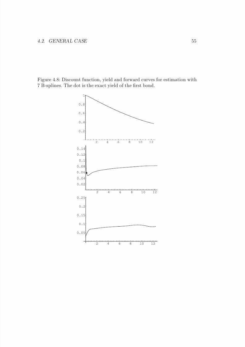
and the discount function, yield curve (cont. comp. spot rates), and
forward curve (cont. comp. 3-month forward rates) shown in Figure 4.8.
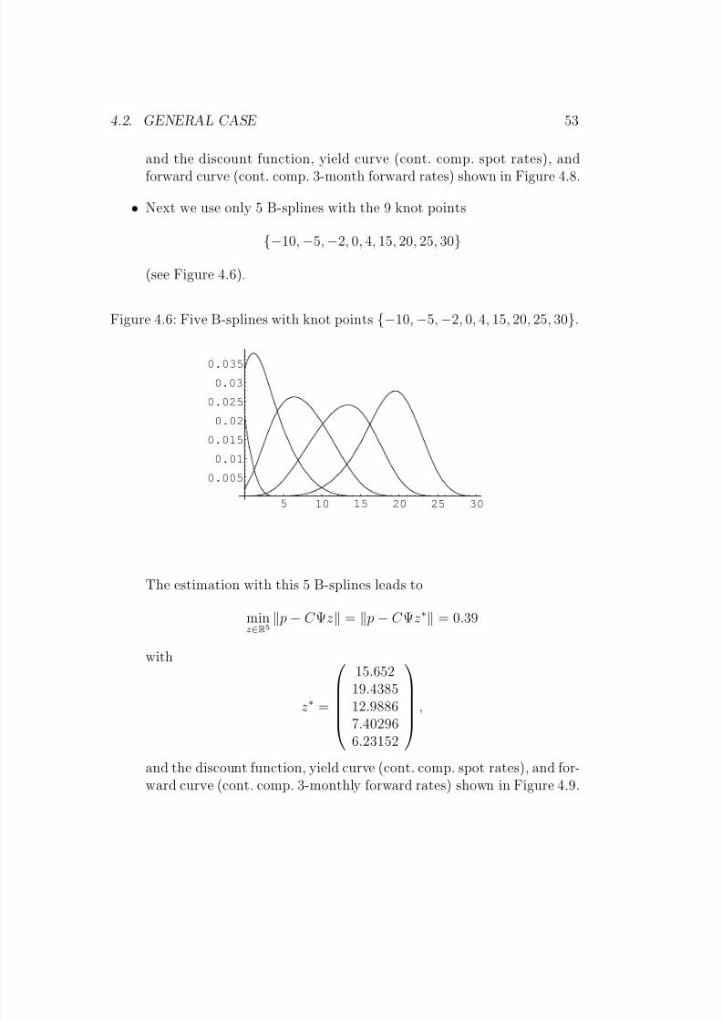
• Next we use only 5 B-splines with the 9 knot points
−10, −5, −2, 0, 4, 15, 20, 25, 30
(see Figure 4.6).
Figure 4.6: Five B-splines with knot points −10, −5, −2, 0, 4, 15, 20, 25, 30.
5 10 15 20 25 30
0.005
0.01
0.015
0.02
0.025
0.03
0.035
The estimation with this 5 B-splines leads to
minz∈R5
p − C Ψz = p − C Ψz∗ = 0.39
with
z∗ =
15.65219.438512.98867.402966.23152
,
and the discount function, yield curve (cont. comp. spot rates), and for-ward curve (cont. comp. 3-monthly forward rates) shown in Figure 4.9.

8/7/2019 Fixed Income Models
http://slidepdf.com/reader/full/fixed-income-models 54/167
54 CHAPTER 4. ESTIMATING THE YIELD CURVE
Figure 4.7: Discount function, yield and forward curves for estimation with8 B-splines. The dot is the exact yield of the first bond.
2 4 6 8 10 12
0.2
0.4
0.6
0.8
1
2 4 6 8 10 12
0.02
0.04
0.06
0.08
0.1
0.12
0.14
2 4 6 8 10 12
0.05
0.1
0.15
0.2
0.25
8/7/2019 Fixed Income Models
http://slidepdf.com/reader/full/fixed-income-models 55/167
4.2. GENERAL CASE 55
Figure 4.8: Discount function, yield and forward curves for estimation with7 B-splines. The dot is the exact yield of the first bond.
2 4 6 8 10 12
0.2
0.4
0.6
0.8
1
2 4 6 8 10 12
0.02
0.04
0.06
0.08
0.1
0.12
0.14
2 4 6 8 10 12
0.05
0.1
0.15
0.2
0.25

8/7/2019 Fixed Income Models
http://slidepdf.com/reader/full/fixed-income-models 56/167
56 CHAPTER 4. ESTIMATING THE YIELD CURVE
Figure 4.9: Discount function, yield and forward curves for estimation with5 B-splines. The dot is the exact yield of the first bond.
2 4 6 8 10 12
0.2
0.4
0.6
0.8
1
2 4 6 8 10 12
0.02
0.04
0.06
0.08
0.1
0.12
0.14
2 4 6 8 10 12
0.05
0.1
0.15
0.2
0.25

8/7/2019 Fixed Income Models
http://slidepdf.com/reader/full/fixed-income-models 57/167
4.2. GENERAL CASE 57
Discussion
• In general, splines can produce bad fits.
• Estimating the discount function leads to unstable and non-smoothyield and forward curves. Problems mostly at short and long termmaturities.
• Splines are not useful for extrapolating to long term maturities.
• There is a trade-off between the quality (or regularity) and the correct-ness of the fit. The curves in Figures 4.8 and 4.9 are more regular thanthose in Figure 4.7, but their correctness criteria (0.32 and 0.39) are
worse than for the fit with 8 B-splines (0.23).
• The B-spline fits are extremely sensitive to the number and location of the knot points.
→ Need criterions asserting smooth yield and forward curves that do notfluctuate too much and flatten towards the long end.
→ Direct estimation of the yield or forward curve.
→ Optimal selection of number and location of knot points for splines.
→ Smoothing splines.
Smoothing Splines The least squares criterion
minz
p − C · d(z)2
has to be replaced/extended by criterions for the smoothness of the yield orforward curve.
Example: Lorimier (95). In her PhD thesis 1995, Sabine Lorimier sug-gests a spline method where the number and location of the knots are deter-mined by the observed data itself.
For ease of notation we set t0 = 0 (today). The data is given by N observed zero-coupon bonds P (0, T 1), . . . , P (0, T N ) at 0 < T 1 < · · · < T N ≡T , and consequently the N yields
Y 1, . . . , Y N , P (0, T i) = exp(−T iY i).
8/7/2019 Fixed Income Models
http://slidepdf.com/reader/full/fixed-income-models 58/167
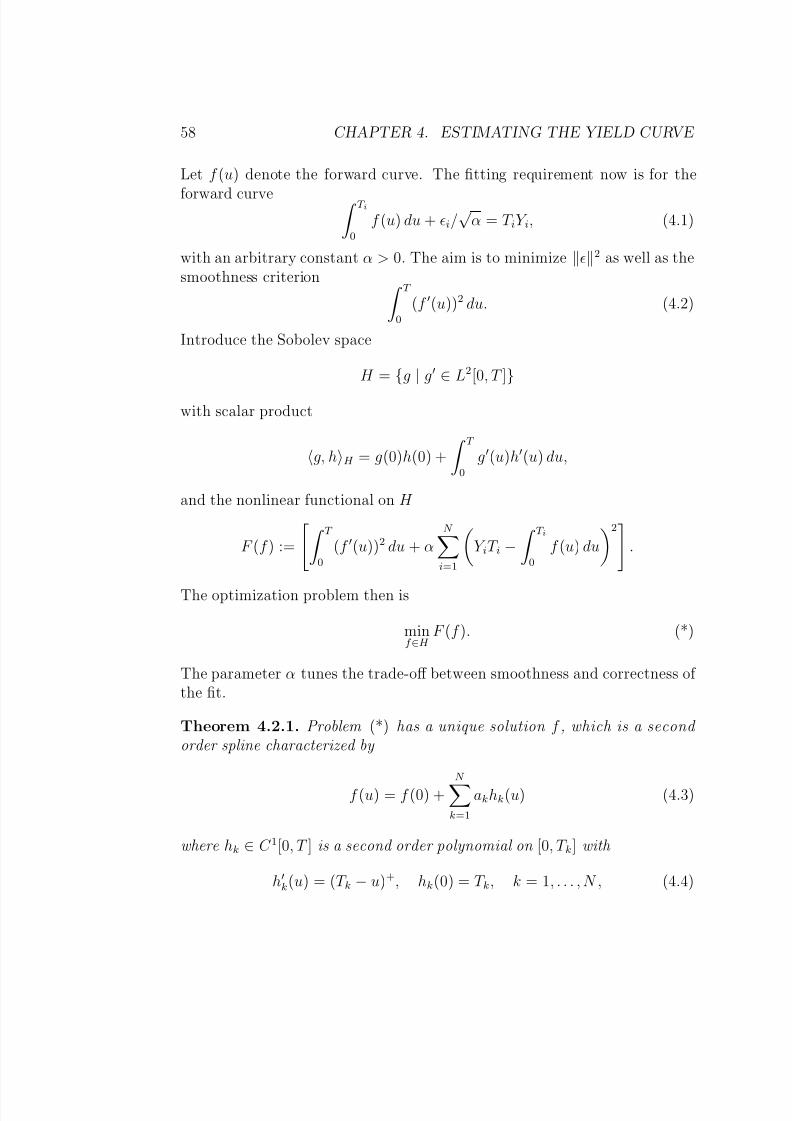
58 CHAPTER 4. ESTIMATING THE YIELD CURVE
Let f (u) denote the forward curve. The fitting requirement now is for the
forward curve T i0
f (u) du + i/√
α = T iY i, (4.1)
with an arbitrary constant α > 0. The aim is to minimize 2 as well as thesmoothness criterion T
0
(f (u))2 du. (4.2)
Introduce the Sobolev space
H =
g
|g
∈L2[0, T ]
with scalar product
g, hH = g(0)h(0) +
T 0
g(u)h(u) du,
and the nonlinear functional on H
F (f ) :=
T 0
(f (u))2 du + αN i=1
Y iT i −
T i0
f (u) du
2
.
The optimization problem then is
minf ∈H
F (f ). (*)
The parameter α tunes the trade-off between smoothness and correctness of the fit.
Theorem 4.2.1. Problem (*) has a unique solution f , which is a second order spline characterized by
f (u) = f (0) +N k=1
akhk(u) (4.3)
where hk ∈ C 1[0, T ] is a second order polynomial on [0, T k] with
hk(u) = (T k − u)+, hk(0) = T k, k = 1, . . . , N , (4.4)

8/7/2019 Fixed Income Models
http://slidepdf.com/reader/full/fixed-income-models 59/167
4.2. GENERAL CASE 59
and f (0) and ak solve the linear system of equations
N k=1
akT k = 0, (4.5)
α
Y kT k − f (0)T k −
N l=1
alhl, hkH
= ak, k = 1, . . . , N . (4.6)
Proof. Integration by parts yields
T k
0
g(u) du = T kg(T k) − T k
0
ug(u) du
= T kg(0) + T k
T k0
g(u) du − T k
0
ug(u) du
= T kg(0) +
T 0
(T k − u)+g(u) du = hk, gH ,
for all g ∈ H . In particular, T k0
hl du = hl, hkH .
A (local) minimizer f of F satisfies
d
dF (f + g)|=0 = 0
or equivalently
T 0
f g du = αN k=1
Y kT k −
T k0
f du
T k0
gdu, ∀g ∈ H. (4.7)
In particular, for all g
∈H with
g, hk
H = 0 we obtain
f − f (0), gH = T
0
f (u)g(u) du = 0.
Hencef − f (0) ∈ spanh1, . . . , hN

8/7/2019 Fixed Income Models
http://slidepdf.com/reader/full/fixed-income-models 60/167
8/7/2019 Fixed Income Models
http://slidepdf.com/reader/full/fixed-income-models 61/167
4.2. GENERAL CASE 61
Multiplying the latter equation with λk and summing up yields
α
N k=1
λkhk
2
H
+N k=1
λ2k = 0.
Hence λ = 0, whence A is non-singular.
The role of α is as follows:
• If α → 0 then by (4.3) and (4.6) we have f (u) ≡ f (0), a constantfunction. That is, maximal regularity
T 0
(f (u))2 du = 0
but no fitting of data, see (4.1).
• If α → ∞ then (4.7) implies that T k0
f (u) du = Y kT k, k = 1, . . . , N , (4.9)
a perfect fit. That is, f minimizes (4.2) subject to the constraints (4.9).
To estimate the forward curve from N zero-coupon bonds—that is, yieldsY = (Y 1, . . . , Y N )T —one has to solve the linear system
A ·
f (0)a
=
0Y
(see (4.8)).
Of course, if coupon bond prices are given, then the above method hasto be modified and becomes nonlinear. With p ∈ Rn denoting the marketprice vector and ckl the cashflows at dates T l, k = 1, . . . , n, l = 1, . . . , N , thisreads
minf ∈H
T
0(f )2 du + α
nk=1
log pk − log N l=1
ckl exp − T l0
f du2 .
If the coupon payments are small compared to the nominal (=1), then thisproblem has a unique solution. This and much more is carried out in Lorim-ier’s thesis.

8/7/2019 Fixed Income Models
http://slidepdf.com/reader/full/fixed-income-models 62/167
62 CHAPTER 4. ESTIMATING THE YIELD CURVE
Exponential-Polynomial Families
Exponential-polynomial functions
p1(x)e−α1x + · · · + pn(x)e−αnx ( pi=polynomial of degree ni)
form non-linear families of functions. Popular examples are:
Nelson–Siegel (87) [20] There are 4 parameters z1, . . . , z4 and
φNS (x; z) = z1 + (z2 + z3x)e−z4x.
Svensson (94) [26] (Prof. L. E. O. Svensson is at the Economics Depart-ment, Princeton University) This is an extension of Nelson–Siegel, in-cluding 6 parameters z1, . . . , z6,
φS (x; z) = z1 + (z2 + z3x)e−z4x + z5e−z6x.
Figure 4.10: Nelson–Siegel curves for z1 = 7.69, z2 =
−4.13, z4 = 0.5 and 7
different values for z3 = 1.76, 0.77, −0.22, −1.21, −2.2, −3.19, −4.18.
5 10 15 20
2
4
6
8
Table 4.4 is taken from a document of the Bank for International Settle-ments (BIS) 1999 [2].

8/7/2019 Fixed Income Models
http://slidepdf.com/reader/full/fixed-income-models 63/167
4.2. GENERAL CASE 63
Table 4.4: Overview of estimation procedures by several central banks. BIS
1999 [2]. NS is for Nelson–Siegel, S for Svensson, wp for weighted prices.
Central Bank Method Minimized Error
Belgium S or NS wpCanada S spFinland NS wpFrance S or NS wp
Germany S yieldsItaly NS wp
Japan smoothing prices
splinesNorway S yields
Spain S wpSweden S yields
UK S yieldsUSA smoothing bills: wp
splines bonds: prices
Criteria for Curve Families
• Flexibility (do the curves fit a wide range of term structures?)
• Number of factors not too large (curse of dimensionality).
• Regularity (smooth yield or forward curves that flatten out towards thelong end).
• Consistency: do the curve families go well with interest rate models?→ this point will be exploited in the sequel.

8/7/2019 Fixed Income Models
http://slidepdf.com/reader/full/fixed-income-models 64/167
64 CHAPTER 4. ESTIMATING THE YIELD CURVE
8/7/2019 Fixed Income Models
http://slidepdf.com/reader/full/fixed-income-models 65/167
Chapter 5
Why Yield Curve Models?
→ R[22](Chapter 5)Why modelling the entire term structure of interest rates? There is no
need when pricing a single European call option on a bond.
But: the payoffs even of “plain-vanilla” fixed income products such as caps,floors, swaptions consist of a sequence of cashflows at T 1, . . . , T n, wheren may be 20 (e.g. a 10y swap with semi-annual payments) or more.
→ The valuation of such products requires the modelling of the entire covari-ance structure. Historical estimation of such large covariance matrices
is statistically not tractable anymore.
→ Need strong structure to be imposed on the co-movements of financialquantities of interest.
→ Specify the dynamics of a small number of variables (e.g. PCA).
→ Correlation structure among observable quantities can now be obtainedanalytically or numerically.
→ Simultaneous pricing of different options and hedging instruments in aconsistent framework.
This is exactly what interest rate (curve) models offer:
• reduction of fitting degrees of freedom → makes problem manageable.
=⇒ It is practically and intellectually rewarding to consider no-arbitrageconditions in much broader generality.
65

8/7/2019 Fixed Income Models
http://slidepdf.com/reader/full/fixed-income-models 66/167

8/7/2019 Fixed Income Models
http://slidepdf.com/reader/full/fixed-income-models 67/167
Chapter 6
No-Arbitrage Pricing
This chapter briefly recalls the basics about pricing and hedging in a Brown-ian motion driven market. Reference is B[3], MR[19](Chapter 10), and manymore.
6.1 Self-Financing Portfolios
The stochastic basis is a probability space (Ω, F ,P), a d-dimensional Brow-nian motion W = (W 1, . . . , W d), and the filtration (F t)t≥0 generated by W .
We shall assume that F = F ∞ = ∨t≥0F t, and do not a priori fix a finitetime horizon. This is not a restriction since always one can set a stochasticprocess to be zero after a finite time T if this were the ultimate time horizon(as in the Black–Scholes model).
The background for stochastic analysis can be found in many textbooks,such as [14], [25], [23], etc. From time to time we recall some of the funda-mental results without proof.
Financial Market We consider a financial market with n traded assets,following strictly positive Ito processes
dS i(t) = S i(t)µi(t) dt +d
j=1
S i(t)σij(t) dW j(t), S i > 0, i = 1, . . . , n
and the risk-free asset
dS 0(t) = r(t)S 0(t) dt, S 0(0) = 1⇔ S 0(t) = e
t0r(s)ds
.
67
8/7/2019 Fixed Income Models
http://slidepdf.com/reader/full/fixed-income-models 68/167
68 CHAPTER 6. NO-ARBITRAGE PRICING
The drift µ = (µ1, . . . , µn), volatility σ = (σij), and short rates r are assumed
to form adapted processes which meet the required integrability conditionssuch that all of the above (stochastic) integrals are well-defined.
Remark 6.1.1. It is always understood that for a random variable “ X ≥ 0”means “ X ≥ 0 a.s.” (that is, P[X ≥ 0] = 1), etc.
Theorem 6.1.2 (Stochastic Integrals). Let h = (h1, . . . , hd) be a mea-surable adapted process. If t
0
h(s)2 ds < ∞ for all t > 0
(the class of such processes is denoted by L) one can define the stochasticintegral
(h · W )t ≡ t
0
h(s) dW (s) ≡d
j=1
t0
h j(s) dW j(s).
If moreover
E
∞0
h(s)2 ds
< ∞
(the class of such processes is denoted by L2) then h · W is a martingale and the Ito isometry holds
E
t0
h(s) dW (s)
2
= E
t0
h(s)2 ds
.
Self-financing Portfolios A portfolio, or trading strategy , is any adaptedprocess
φ = (φ0, . . . , φn).
Its corresponding value process is
V (t) = V (t; φ) :=
ni=0
φi(t)S i(t).
The portfolio φ is called self-financing (for S ) if the stochastic integrals t0
φi(u) dS i(u), i = 0, . . . , n

8/7/2019 Fixed Income Models
http://slidepdf.com/reader/full/fixed-income-models 69/167
6.2. ARBITRAGE AND MARTINGALE MEASURES 69
are well defined and
dV (t; φ) =
ni=0
φi(t) dS i(t).
Numeraires All prices are interpreted as being given in terms of a nu-meraire, which typically is a local currency such as US dollars. But we mayand will express from time to time the prices in terms of other numeraires,such as S p for some 0 ≤ p ≤ n. The discounted price process vector
Z (t) :=S (t)
S p(t)
implies the discounted value process
V (t; φ) :=ni=0
φi(t)Z i(t) =V (t; φ)
S p(t).
Up to integrability, the self-financing property does not depend on the choiceof the numeraire.
Lemma 6.1.3. Suppose that a portfolio φ satisfies the integrability conditions for S and Z . Then φ is self-financing for S if and only if it is self-financing for Z , in particular
dV (t; φ) =ni=0
φi(t) dZ i(t) =ni=0i=p
φi(t) dZ i(t). (6.1)
Since Z p is constant, the number of terms in (6.1) reduces to n.Often (but not always) we chose S 0 as the numeraire.
6.2 Arbitrage and Martingale Measures
Contingent Claims Related to any option (such as a cap, floor, swaption,
etc) is an uncertain future payoff, say at date T , hence an F T -measurablerandom variable X (a contingent ( T -)claim ). Two main problems now are:
• What is a “fair” price for a contingent claim X ?
• How can one hedge against the financial risk involved in trading con-tingent claims?

8/7/2019 Fixed Income Models
http://slidepdf.com/reader/full/fixed-income-models 70/167
70 CHAPTER 6. NO-ARBITRAGE PRICING
Arbitrage An arbitrage portfolio is a self-financing portfolio φ with value
process satisfying
V (0) = 0 and V (T ) ≥ 0 and P[V (T ) > 0] > 0
for some T > 0. If no arbitrage portfolios exist for any T > 0 we say themodel is arbitrage-free.
An example of arbitrage is the following.
Lemma 6.2.1. Suppose there exists a self-financing portfolio with value pro-cess
dU (t) = k(t)U (t) dt, for some measurable adapted process k. If the market is arbitrage-free then necessarily
r = k, dt ⊗ dP-a.s.
Proof. Indeed, after discounting with S 0 we obtain
U (t) :=U (t)
S 0(t)= U (0) exp
t0
(k(s) − r(s)) ds
.
Then (→
exercise)ψ(t) := 1k(t)>r(t)
yields a self-financing strategy with discounted value process
V (t) =
t0
ψ(s) dU (s) =
t0
1k(s)>r(s)(k(s) − r(s))U (s)
ds ≥ 0.
Hence absence of arbitrage requires
0 = E[V (T )] =
N
1k(t,ω)>r(t,ω)(k(t, ω) − r(t, ω))U (t, ω)
>0 on N
dt ⊗ dP
where N := (t, ω) | k(t, ω) > r(t, ω)
is a measurable subset of [0, T ]× Ω. But this can only hold if N is a dt ⊗dP-nullset. Using the same arguments with changed signs proves the lemma.
8/7/2019 Fixed Income Models
http://slidepdf.com/reader/full/fixed-income-models 71/167

8/7/2019 Fixed Income Models
http://slidepdf.com/reader/full/fixed-income-models 72/167
72 CHAPTER 6. NO-ARBITRAGE PRICING
Hence necessarily γ satisfies
µi − r + σi · γ = 0 dt ⊗ dQ-a.s. for all i = 1, . . . , n. (6.5)
If σ is non-degenerate (in particular d ≤ n and rank[σ] = d) then γ isuniquely specified by
−γ = σ−1 · (µ − r1)
where 1 := (1, . . . , 1)T , and vice versa. This is why −γ is called the market price of risk .
Conversely, if (6.5) has a solution γ ∈ L such that E (γ ·W ) is a uniformlyintegrable martingale (the Novikov condition (6.4) is sufficient) then (6.2)defines an ELMM Q. If γ is unique then Q is the unique ELMM.
Notice that, by Ito’s formula, Z i can be written as stochastic exponentialZ i = E (σi · W ).
Hence if σi satisfies the Novikov condition (6.4) for all i = 1, . . . , n then theELMM Q is in fact an EMM.
Admissible Strategies In the presence of local martingales one has to bealert to pitfalls. For example it is possible to construct a local martingale M with M (0) = 0 and M (1) = 1. Even worse, M can be chosen to be of theform
M (t) = t
0
φ(s) dW (s)
(Dudley’s Representation Theorem), which looks like the (discounted) valueprocess of a self-financing strategy. This would certainly be a money-makingmachine, say arbitrage. In the same way “suicide strategies” (e.g. M (0) = 1and M (1) = 0) can be constructed. To rule out such examples we have toimpose additional constraints on the choice of strategies. There are severalways to do so. Here are two typical examples:
A self-financing strategy φ is admissible if
1. V (t; φ) ≥ −a for some a ∈ R, OR
2.˜V (t; φ) is a true Q-martingale, for some ELMM Q.
Condition 1 is more universal (it does not depend on a particular Q) andimplies that V (t; φ) is a Q-supermartingale for every ELMM Q. Yet, “suicidestrategies” remain (however, they do not introduce arbitrage).
Both conditions 1 and 2, however, are sensitive with respect to the choiceof numeraire!

8/7/2019 Fixed Income Models
http://slidepdf.com/reader/full/fixed-income-models 73/167
6.3. HEDGING AND PRICING 73
The Fundamental Theorem of Asset Pricing The existence of an
ELMM rules out arbitrage.
Lemma 6.2.3. Suppose there exists an ELMM Q. Then the model is arbi-trage-free, in the sense that there exists no admissible (either Condition 1 or 2) arbitrage strategy.
Proof. Indeed, let V be the discounted value process of an admissible strat-egy, with V (0) = 0 and V (T ) ≥ 0. Since V is a Q-supermartingale in anycase (for some ELMM Q), we have
0 ≤ EQ[˜V (T )] ≤
˜V (0) = 0,
whence V (T ) = 0.
It is folklore (Delbaen and Schachermayer 1994, etc) that also the converseholds true: if arbitrage is defined in the right way (“No Free Lunch withVanishing Risk”), then its absence implies the existence of an ELMM Q.This is called the Fundamental Theorem of Asset Pricing .
It has become a custom (and we will follow this tradition) to consider theexistence of an ELMM as synonym for the absence of arbitrage:
absence of arbitrage = existence of an ELMM;
→ the existence of an ELMM is now a standing assumption.
6.3 Hedging and Pricing
Attainable Claims A contingent claim X due at T is attainable if theexists an admissible strategy φ which replicates/hedges X ; that is,
V (T ; φ) = X.
A simple example: suppose S 1 is the price process of the T -bond. Thenthe contingent claim X = 1 due at T is attainable by an obvious buy andhold strategy with value process V (t) = S 1(t).

8/7/2019 Fixed Income Models
http://slidepdf.com/reader/full/fixed-income-models 74/167

8/7/2019 Fixed Income Models
http://slidepdf.com/reader/full/fixed-income-models 75/167
6.3. HEDGING AND PRICING 75
Now define
φi = ((σ−1
)T ˜
ψ)iZ i
, (6.8)
then it follows thatni=1
φi dZ i =ni=1
φiZ iσi dW = (σ−1)T ψ · σ dW = ψ · σ−1σ dW = ψ dW = dY .
Hence φ yields an admissible strategy with discounted value process satisfying
V (T ; φ) = Y (T ) = EQ [X/S 0(T )] +ni=1
T 0
φi(s) dZ i(s) = X/S 0(T ). (6.9)
Hence non-degeneracy of σ (see (6.6) and (6.8)) implies uniqueness of Qand completeness of the model. These conditions are in fact equivalent (seefor example MR[19](Chapter 10)).
Theorem 6.3.2 (Completeness). The following are equivalent:
1. the model is complete;
2. σ is non-degenerate, see (6.6);
3. there exists a unique ELMM Q
.Theorem 6.3.3 (Representation Theorem). Every P-local martingaleM has a continuous version and there exists ψ ∈ L such that
M (t) = M (0) +
t0
ψ(s) dW (s).
(This theorem requires the filtration (F t) to be generated by W .)
Pricing In the above complete model the fair price prevailing at t ≤ T of a T -claim X which satisfies (6.7) is given by (6.9)
V (t, φ) = S 0(t)V (t; φ) = S 0(t)EQ [X/S 0(T ) | F t] . (6.10)
We shall often encounter complete models. However, models can be gener-ically incomplete (as real markets are), and then the pricing becomes a dif-ficult issue. The literature on incomplete markets is huge, and the topicbeyond the scope of this course.

8/7/2019 Fixed Income Models
http://slidepdf.com/reader/full/fixed-income-models 76/167
76 CHAPTER 6. NO-ARBITRAGE PRICING
State-price Density It is a custom (e.g. for short rate models) to exoge-
nously specify a particular ELMM Q (or equivalently, the market price of risk) and then price a T -claim X satisfying (6.7) according to (6.10)
price of X at t =: Y (t) = S 0(t)EQ [X/S 0(T ) | F t] .
This is a consistent pricing rule in the sense that the enlarged market
Y, S 0, . . . , S n
is still arbitrage-free (why?).Now define
π(t) :=1
S 0(t)
dQ
dP |F t .By Bayes formula we then have
Y (t) = S 0(t)EQ [X/S 0(T ) | F t] = S 0(t)E
X
S 0(T )dQdP
|F T | F t
dQdP
|F t=E [Xπ(T ) | F t]
π(t),
and, in particular, for the price at t = 0
Y (0) = E[Xπ(T )].
This is why π is called the state-price density process.The price of a T -bond for example is (if 1/S 0(T ) ∈ L1(Q), → exercise)
P (t, T ) = E
π(T )
π(t)| F t
= EQ
S 0(t)
S 0(T )| F t
.
Also one can check (→ exercise) that if Q is an EMM then
S iπ are P-martingales.

8/7/2019 Fixed Income Models
http://slidepdf.com/reader/full/fixed-income-models 77/167
Chapter 7
Short Rate Models
→ B[3](Chapters 16–17), MR[19](Chapter 12), etc
7.1 Generalities
Short rate models are the classical interest rate models. As in the last sec-tion we fix a stochastic basis (Ω, F ,P), where P is considered as objectiveprobability measure. The filtration (F t)t≥0 is generated by a d-dimensionalBrownian motion W .
We assume that
• the short rates follow an Ito process
dr(t) = b(t) dt + σ(t) dW (t)
determining the savings account B(t) = exp t
0r(s) ds
,
• all zero-coupon bond prices (P (t, T ))t∈[0,T ] are adapted processes (withP (T, T ) = 1 as usual),
• no-arbitrage: there exists an EMM Q, such that
P (t, T )
B(t), t ∈ [0, T ],
is a Q-martingale for all T > 0.
77

8/7/2019 Fixed Income Models
http://slidepdf.com/reader/full/fixed-income-models 78/167
78 CHAPTER 7. SHORT RATE MODELS
According to the last chapter, the existence of an ELMM for all T -bonds
excludes arbitrage among every finite selection of zero-coupon bonds, sayP (t, T 1), . . . , P (t, T n). To be more general one would have to consider strate-gies involving a continuum of bonds. This can be done (see [4] or MikeTehranchi’s PhD thesis 2002) but is beyond the scope of this course.
For convenience we require Q to be an EMM (and not merely an ELMM)because then we have
P (t, T ) = EQ
e−
T t r(s)ds | F t
(7.1)
(compare this to the last section). Let −γ denote the corresponding market
price of risk E t(γ · W ) =dQ
dP|F t
and W = W − γ dt the implied Q-Brownian motion.
Proposition 7.1.1. Under the above assumptions, the process r satisfiesunder Q
dr(t) = (b(t) + σ(t) · γ (t)) dt + σ(t) dW (t). (7.2)
Moreover, for any T > 0 there exists an adapted Rd-valued process σγ (t, T ),t ∈ [0, T ], such that
dP (t, T )
P (t, T )= r(t) dt + σγ (t, T ) dW (t) (7.3)
and henceP (t, T )
B(t)= P (0, T )E t
σγ · W
.
Proof. Exercise (proceed as in the Completeness Lemma 6.3.1).
It follows from (7.3) that the T -bond price satisfies under the objectiveprobability measure P
dP (t, T )
P (t, T )= (r(t) − γ (t) · σγ (t, T )) dt + σγ dW (t).
This illustrates again the role of the market price of risk −γ as the excess of instantaneous return over r(t) in units of volatility.

8/7/2019 Fixed Income Models
http://slidepdf.com/reader/full/fixed-income-models 79/167
7.2. DIFFUSION SHORT RATE MODELS 79
In a general equilibrium framework, the market price of risk is given
endogenously (as it is carried out in the seminal paper by Cox, Ingersoll andRoss (85) [7]). Since our arguments refer only to the absence of arbitragebetween primary securities (bonds) and derivatives, we are unable to identifythe market price of risk. In other words, we started by specifying the P-dynamics of the short rates, and hence the savings account B(t). However,the savings account alone cannot be used to replicate bond payoffs: themodel is incomplete. According to the Completeness Theorem 6.3.2, this isalso reflected by the non-uniqueness of the EMM (the market price of risk).A priori, Q can be any equivalent probability measure Q ∼ P.
A short rate model is not fully determined without the exogenous
specification of the market price of risk.
It is custom (and we follow this tradition) to postulate the Q-dynamics(Q being the EMM) of r which implies the Q-dynamics of all bond pricesby (7.1), see also (7.3). All contingent claims can be priced by taking Q-expectations of their discounted payoffs. The market price of risk (and hencethe objective measure P) can be inferred by statistical methods from histor-ical observations of price movements.
7.2 Diffusion Short Rate ModelsWe fix a stochastic basis (Ω, F , (F t)t≥0,Q), where now Q is considered asmartingale measure. We let W denote a d-dimensional (Q, F t)-Brownianmotion.
Let Z ⊂ R be a closed interval, and b and σ continuous functions onR+ × Z . We assume that for any ρ ∈ Z the stochastic differential equation(SDE)
dr(t) = b(t, r(t)) dt + σ(t, r(t)) dW (t) (7.4)
admits a unique Z -valued solution r = rρ with
r(t) = ρ + t
0
b(u, r(u)) du + t
0
σ(u, r(u)) dW (u)
and such that
exp
− T t
r(u) du
∈ L1(Q) (7.5)

8/7/2019 Fixed Income Models
http://slidepdf.com/reader/full/fixed-income-models 80/167
80 CHAPTER 7. SHORT RATE MODELS
for all 0 ≤ t ≤ T . Notice that (7.5) is always satisfied if Z ⊂ R+.
Sufficient for the existence and uniqueness is Lipschitz continuity of b(t, r)and σ(t, r) in r, uniformly in t. If d = 1 then Holder continuity of order 1/2of σ in r, uniformly in t, is enough. A good reference for SDEs is the bookof Karatzas and Shreve [14] on Brownian motion and stochastic calculus.
Condition (7.5) allows us to define the T -bond prices
P (t, T ) = EQ
exp
− T t
r(u) du
| F t
.
It turns out that P (t, T ) can be written as a function of r(t), t and T . This isa general property of certain functionals of Markov process, usually referredto as Feynman–Kac formula. In the following we write
a(t, r) :=σ(t, r)2
2
for the diffusion term of r(t).
Lemma 7.2.1. Let T > 0 and Φ be a continuous function on Z , and assumethat F = F (t, r) ∈ C 1,2([0, T ]×Z ) is a solution to the boundary value problem on [0, T ] × Z
∂ tF (t, r) + b(t, r)∂ rF (t, r) + a(t, r)∂ 2rF (t, r) − rF (t, r) = 0
F (T, r) = Φ(r).(7.6)
Then
M (t) = F (t, r(t))e− t0r(u) du, t ∈ [0, T ],
is a local martingale. If in addition either
1. ∂ rF (t, r(t))e− t0r(u) duσ(t, r(t)) ∈ L2[0, T ], or
2. M is uniformly bounded,
then M is a true martingale, and
F (t, r(t)) = EQ
exp
− T t
r(u) du
Φ(r(T )) | F t
, t ≤ T. (7.7)

8/7/2019 Fixed Income Models
http://slidepdf.com/reader/full/fixed-income-models 81/167
7.2. DIFFUSION SHORT RATE MODELS 81
Proof. We can apply Ito’s formula to M and obtain
dM (t) =
∂ tF (t, r(t)) + b(t, r(t))∂ rF (t, r(t))
+ a(t, r)∂ 2rF (t, r(t)) − r(t)F (t, r(t))
e− t0r(u)du dt
+ ∂ rF (t, r(t))e− t0r(u)duσ(t, r(t)) dW (t)
= ∂ rF (t, r(t))e− t0r(u)duσ(t, r(t)) dW (t).
Hence M is a local martingale.It is now clear that either Condition 1 or 2 imply that M is a true mar-
tingale. Since
M (T ) = Φ(r(T ))e− T 0 r(u) du
we get
F (t, r(t))e− t0r(u) du = M (t) = EQ
exp
− T
0
r(u) du
Φ(r(T )) | F t
.
Multiplying with e t0r(u) du yields the claim.
We call (7.6) the term structure equation for Φ. Its solution F gives theprice of the T -claim Φ(r(T )). In particular, for Φ
≡1 we get the T -bond
price P (t, T ) as a function of t, r(t) (and T )
P (t, T ) = F (t, r(t); T ).
Remark 7.2.2. Strictly speaking, we have only shown that if a smooth solu-tion F of (7.6) exists and satisfies some additional properties (Condition 1or 2) then the time t price of the claim Φ(r(T )) (which is the right hand sideof (7.7)) equals F (t, r(t)). One can also show the converse that the expecta-tion on the right hand side of (7.7) conditional on r(t) = r can be written asF (t, r) where F solves the term structure equation (7.6) but usually only in a weak sense, which in particular means that F may not be in C 1,2([0, T ]
×Z ).
This is general Markov theory and we will not prove this here.
In any case, we have found a pricing algorithm. Is it computationallyefficient? Solving PDEs numerically in more than three dimensions causesdifficulties. PDEs in less than three space dimensions are numerically feasi-ble, and the dimension of Z is one. The nuisance is that we have to solve a

8/7/2019 Fixed Income Models
http://slidepdf.com/reader/full/fixed-income-models 82/167
82 CHAPTER 7. SHORT RATE MODELS
PDE for every single zero-coupon bond price function F (·, ·; T ), T > 0. From
that we might want to derive the yield or even forward curve. If we do notimpose further structural assumptions we may run into regularity problems.Hence
short rate models that admit closed form solutions to the termstructure equation (7.6), at least for Φ ≡ 1, are favorable.
7.2.1 Examples
This is a (far from complete) list of the most popular short rate models. Forall examples we have d = 1. If not otherwise stated, the parameters are
real-valued.1. Vasicek (1977): Z = R,
dr(t) = (b + βr(t)) dt + σ dW (t),
2. Cox–Ingersoll–Ross (CIR, 1985): Z = R+, b ≥ 0,
dr(t) = (b + βr(t)) dt + σ
r(t) dW (t),
3. Dothan (1978): Z = R+,
dr(t) = βr(t) dt + σr(t) dW (t),
4. Black–Derman–Toy (1990): Z = R+,
dr(t) = β (t)r(t) dt + σ(t)r(t) dW (t),
5. Black–Karasinski (1991): Z = R+, (t) = log r(t),
d(t) = (b(t) + β (t)(t)) dt + σ(t) dW (t),
6. Ho–Lee (1986): Z = R,
dr(t) = b(t) dt + σ dW (t),
7. Hull–White (extended Vasicek, 1990): Z = R,
dr(t) = (b(t) + β (t)r(t)) dt + σ(t) dW (t),
8. Hull–White (extended CIR, 1990): Z = R+, b(t) ≥ 0,
dr(t) = (b(t) + β (t)r(t)) dt + σ(t)
r(t) dW (t).

8/7/2019 Fixed Income Models
http://slidepdf.com/reader/full/fixed-income-models 83/167
7.3. INVERTING THE YIELD CURVE 83
7.3 Inverting the Yield Curve
Once the short rate model is chosen, the initial term structure
T → P (0, T ) = F (0, r(0); T )
and hence the initial yield and forward curve are fully specified by the termstructure equation (7.6).
Conversely, one may want to invert the term structure equation (7.6) tomatch a given initial yield curve. Say we have chosen the Vasicek model.Then the implied T -bond price is a function of the current short rate leveland the three model parameters b, β and σ
P (0, T ) = F (0, r(0); T , b , β , σ).
But F (0, r(0); T , b , β , σ) is just a parametrized curve family with three degreesof freedom. It turns out that it is often too restrictive and will provide a poorfit of the current data in terms of accuracy (least squares criterion).
Therefore the class of time-inhomogeneous short rate models (such as theHull–White extensions) was introduced. By letting the parameters depend ontime one gains infinite degree of freedom and hence a perfect fit of any givencurve. Usually, the functions b(t) etc are fully determined by the empiricalinitial yield curve.
7.4 Affine Term Structures
Short rate models that admit closed form expressions for the implied bondprices F (t, r; T ) are favorable.
The most tractable models are those where bond prices are of the form
F (t, r; T ) = exp(−A(t, T ) − B(t, T )r),
for some smooth functions A and B. Such models are said to provide anaffine term structure (ATS). Notice that F (T, r; T ) = 1 implies
A(T, T ) = B(T, T ) = 0.
The nice thing about ATS models is that they can be completely character-ized.
8/7/2019 Fixed Income Models
http://slidepdf.com/reader/full/fixed-income-models 84/167
84 CHAPTER 7. SHORT RATE MODELS
Proposition 7.4.1. The short rate model (7.4) provides an ATS only if its
diffusion and drift terms are of the form
a(t, r) = a(t) + α(t)r and b(t, r) = b(t) + β (t)r, (7.8)
for some continuous functions a,α,b,β . The functions A and B in turn satisfy the system
∂ tA(t, T ) = a(t)B2(t, T ) − b(t)B(t, T ), A(T, T ) = 0, (7.9)
∂ tB(t, T ) = α(t)B2(t, T ) − β (t)B(t, T ) − 1, B(T, T ) = 0. (7.10)
Proof. We insert F (t, r; T ) = exp(−A(t, T ) − B(t, T )r) in the term structureequation (7.6) and obtain
a(t, r)B2(t, T ) − b(t, r)B(t, T ) = ∂ tA(t, T ) + (∂ tB(t, T ) + 1)r. (7.11)
The functions B(t, ·) and B2(t, ·) are linearly independent since otherwiseB(t, ·) ≡ B(t, t) = 0, which trivially would lead to be above results witha(t) = α(t) ≡ 0. Hence we can find T 1 > T 2 > t such that the matrix
B2(t, T 1) −B(t, T 1)B2(t, T 2) −B(t, T 2)
is invertible. Hence we can solve (7.11) for a(t, r) and b(t, r), which yields(7.8). Replace a(t, r) and b(t, r) by (7.8), so the left hand side of (7.11) reads
a(t)B2(t, T ) − b(t)B(t, T ) +
α(t)B2(t, T ) − β (t)B(t, T )
r.
Terms containing r must match. This proves the claim.
The functions a,α,b,β in (7.8) can be further specified. They have to besuch that a(t, r) ≥ 0 and r(t) does not leave the state space Z . In fact, it canbe shown that every ATS model can be transformed via affine transformationinto one of the two cases
1. Z = R: necessarily α(t) = 0 and a(t) ≥ 0, and b, β are arbitrary. Thisis the (Hull–White extension of the) Vasicek model.
2. Z = R+: necessarily a(t) = 0, α(t) ≥ 0 and b(t) ≥ 0 (otherwise theprocess would cross zero), and β is arbitrary. This is the (Hull–Whiteextension of the) CIR model.
Looking at the list in Section 7.2.1 we see that all short rate models exceptthe Dothan, Black–Derman–Toy and Black–Karasinski models have an ATS.
8/7/2019 Fixed Income Models
http://slidepdf.com/reader/full/fixed-income-models 85/167
7.5. SOME STANDARD MODELS 85
7.5 Some Standard Models
We discuss some of the most common short rate models.→ B[3](Section 17.4), BM[6](Chapter 3)
7.5.1 Vasicek Model
The solution todr = (b + βr) dt + σ dW
is explicitly given by (→ exercise)
r(t) = r(0)eβt
+
b
β eβt − 1+ σeβt t
0 e−βs
dW (s).
It follows that r(t) is a Gaussian process with mean
E [r(t)] = r(0)eβt +b
β
eβt − 1
and variance
V ar[r(t)] = σ2e2βt
t0
e−2βs ds =σ2
2β
e2βt − 1
.
HenceQ[r(t) < 0] > 0,
which is not satisfactory (although this probability is usually very small).Vasicek assumed the market price of risk to be constant, so that also the
objective P-dynamics of r(t) is of the above form.If β < 0 then r(t) is mean-reverting with mean reversion level b/|β |, see
Figure 7.1, and r(t) converges to a Gaussian random variable with meanb/|β | and variance σ2/(2|β |), for t → ∞.
Equations (7.9)–(7.10) become
∂ tA(t, T ) =
σ2
2 B
2
(t, T ) − bB(t, T ), A(T, T ) = 0,∂ tB(t, T ) = −βB(t, T ) − 1, B(T, T ) = 0.
The explicit solution is
B(t, T ) =1
β
eβ (T −t) − 1
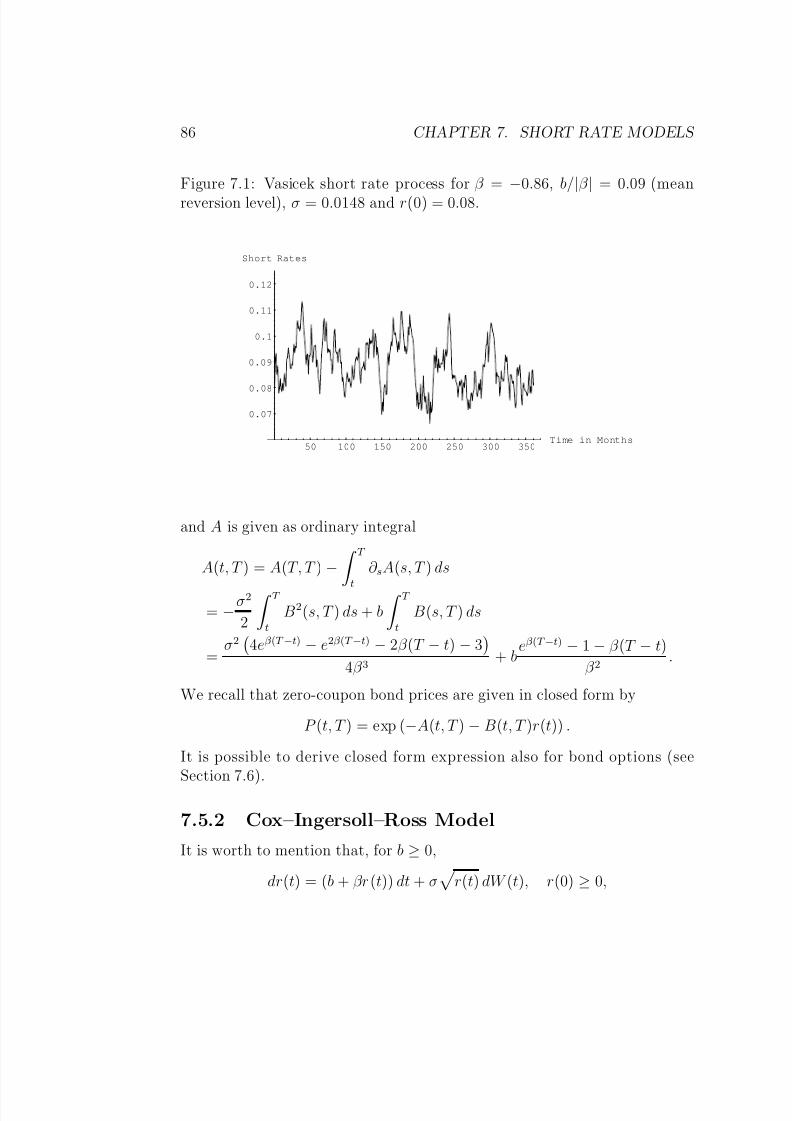
8/7/2019 Fixed Income Models
http://slidepdf.com/reader/full/fixed-income-models 86/167
8/7/2019 Fixed Income Models
http://slidepdf.com/reader/full/fixed-income-models 87/167
7.5. SOME STANDARD MODELS 87
has a unique strong solution r ≥ 0, for every r(0) ≥ 0. This also holds when
the coefficients depend continuously on t, as it is the case for the Hull–Whiteextension. Even more, if b ≥ σ2/2 then r > 0 whenever r(0) > 0.
The ATS equation (7.10) now becomes non-linear
∂ tB(t, T ) =σ2
2B2(t, T ) − βB(t, T ) − 1, B(T, T ) = 0.
This is called a Riccati equation . It is good news that the explicit solution isknown
B(t, T ) =2
eγ (T −t) − 1
(γ − β ) (eγ (T −t) − 1) + 2γ
where γ := β 2
+ 2σ2
. Integration yields
A(t, T ) = − 2b
σ2log
2γe(γ −β )(T −t)/2
(γ − β ) (eγ (T −t) − 1) + 2γ
.
Hence also in the CIR model we have closed form expressions for the bondprices. Moreover, it can be shown that also bond option prices are explicit(!)Together with the fact that it yields positive interest rates, this is mainly thereason why the CIR model is so popular.
7.5.3 Dothan Model
Dothan (78) starts from a drift-less geometric Brownian motion under theobjective probability measure P
dr(t) = σr(t) dW P(t).
The market price of risk is chosen to be constant, which yields
dr(t) = βr(t) dt + σr(t) dW (t)
as Q-dynamics. This is easily integrated
r(t) = r(s)exp β − σ2/2 (t − s) + σ(W (t) − W (s)) , s ≤ t.
Thus the F s-conditional distribution of r(t) is lognormal with mean andvariance (→ exercise)
E[r(t) | F s] = r(s)eβ (t−s)
V ar[r(t) | F s] = r2(s)e2β (t−s)
eσ2(t−s) − 1
.

8/7/2019 Fixed Income Models
http://slidepdf.com/reader/full/fixed-income-models 88/167
88 CHAPTER 7. SHORT RATE MODELS
The Dothan and all lognormal short rate models (Black–Derman–Toy and
Black–Karasinski) yield positive interest rates. But no closed form expres-sions for bond prices or options are available (with one exception: Dothanadmits an “semi-explicit” expression for the bond prices, see BM[6]).
A major drawback of lognormal models is the explosion of the bank ac-count. Let ∆t be small, then
E[B(∆t)] = E
exp
∆t
0
r(s) ds
≈ E
exp
r(0) + r(∆t)
2∆t
.
We face an expectation of the type
E[exp(exp(Y ))]
where Y is Gaussian distributed. But such an expectation is infinite. Thismeans that in arbitrarily small time the bank account growths to infinity inaverage. Similarly, one shows that the price of a Eurodollar future is infinitefor all lognormal models.
The idea of lognormal rates is taken up later by Sandmann and Son-dermann (1997) and many others, which finally led to the so called marketmodels with lognormal LIBOR or swap rates.
7.5.4 Ho–Lee ModelFor the Ho–Lee model
dr(t) = b(t) dt + σ dW (t)
the ATS equations (7.9)–(7.10) become
∂ tA(t, T ) =σ2
2B2(t, T ) − b(t)B(t, T ), A(T, T ) = 0,
∂ tB(t, T ) = −1, B(T, T ) = 0.
Hence
B(t, T ) = T − t,
A(t, T ) = −σ2
6(T − t)3 +
T t
b(s)(T − s) ds.
8/7/2019 Fixed Income Models
http://slidepdf.com/reader/full/fixed-income-models 89/167
7.5. SOME STANDARD MODELS 89
The forward curve is thus
f (t, T ) = ∂ T A(t, T ) + ∂ T B(t, T )r(t) = −σ2
2(T − t)2 +
T t
b(s) ds + r(t).
Let f ∗(0, T ) be the observed (estimated) initial forward curve. Then
b(s) = ∂ sf ∗(0, s) + σ2s.
gives a perfect fit of f ∗(0, T ). Plugging this back into the ATS yields
f (t, T ) = f ∗(0, T ) − f ∗(0, t) + σ2t(T − t) + r(t).
We can also integrate this expression to get
P (t, T ) = e− T tf ∗(0,s) ds+f ∗(0,t)(T −t)−σ2
2t(T −t)2−(T −t)r(t).
It is interesting to see that
r(t) = r(0) +
t0
b(s) ds + σW (t) = f ∗(0, t) +σ2t2
2+ σW (t).
That is, r(t) fluctuates along the modified initial forward curve, and we have
f ∗(0, t) = E[r(t)] −σ2t2
2 .
7.5.5 Hull–White Model
The Hull–White (1990) extensions of Vasicek and CIR can be fitted to theinitial yield and volatility curve. However, this flexibility has its price: themodel cannot be handled analytically in general. We therefore restrict ourself to the following extension of the Vasicek model that was analyzed by Hulland White 1994
dr(t) = (b(t) + βr(t)) dt + σ dW (t).
In this model we choose the constants β and σ to obtain a nice volatilitystructure whereas b(t) is chosen in order to match the initial yield curve.
Equation (7.10) for B(t, T ) is just as in the Vasicek model
∂ tB(t, T ) = −βB (t, T ) − 1, B(T, T ) = 0

8/7/2019 Fixed Income Models
http://slidepdf.com/reader/full/fixed-income-models 90/167
90 CHAPTER 7. SHORT RATE MODELS
with explicit solution
B(t, T ) =1
β
eβ (T −t) − 1
.
Equation (7.9) for A(t, T ) now reads
A(t, T ) = −σ2
2
T t
B2(s, T ) ds +
T t
b(s)B(s, T ) ds
We consider the initial forward curve (notice that ∂ T B(s, T ) = −∂ sB(s, T ))
f ∗(0, T ) = ∂ T A(0, T ) + ∂ T B(0, T )r(0)
=σ2
2
T 0
∂ sB2(s, T ) ds +
T 0
b(s)∂ T B(s, T ) + ∂ T B(0, T )r(0)
= − σ2
2β 2
eβT − 12
=:g(T )
+
T 0
b(s)eβ (T −s) ds + eβT r(0) =:φ(T )
.
The function φ satisfies
∂ T φ(T ) = βφ(T ) + b(T ), φ(0) = r(0).
It follows that
b(T ) = ∂ T φ(T ) − βφ(T )
= ∂ T (f ∗(0, T ) + g(T )) − β (f ∗(0, T ) + g(T )).
Plugging in and performing performing some calculations eventually yields
f (t, T ) = f ∗(0, T ) − eβ (T −t)f ∗(0, t) − σ2
2β 2
eβ (T −t) − 1
eβ (T −t) − eβ (T +t)
+ eβ (T −t)r(t).
7.6 Option Pricing in Affine Models
We show how to price bond options in the affine framework. The discussionis informal, we do not worry about integrability conditions. The procedurehas to be carried out rigorously from case to case.
8/7/2019 Fixed Income Models
http://slidepdf.com/reader/full/fixed-income-models 91/167
7.6. OPTION PRICING IN AFFINE MODELS 91
Let r(t) be a diffusion short rate model with drift
b(t) + β (t)r,
diffusion terma(t) + α(t)r
and ATSP (t, T ) = e−A(t,T )−B(t,T )r(t).
Let λ ∈ C, and φ and ψ be given as solutions to
∂ tφ(t , T, λ) = a(t)ψ2(t , T, λ) − b(t)ψ(t , T, λ)
φ(T , T , λ) = 0
∂ tψ(t , T, λ) = α(t)ψ2(t , T, λ) − β (t)ψ(t , T, λ) − 1
ψ(T , T , λ) = λ.
This looks much like the ATS equations (7.9)–(7.10), and indeed, by pluggingthe right hand side below in the term structure equation (7.6), one sees that
E
e−
T tr(s)dse−λr(T ) | F t
= e−φ(t,T,λ)−ψ(t,T,λ)r(t) .
In fact, we have
φ(t,T, 0) = A(t, T ) and ψ(t,T, 0) = B(t, T ).
Now let t = 0 (for simplicity only). Since discounted zero-coupon bond pricesare martingales we obtain for T ≤ S (→ exercise)
E
e− S0r(s)dse−λr(T )
= E
e−
T 0r(s) dse−A(T,S )−B(T,S )r(T )e−λr(T )
= e−A(T,S )E
e−
T 0r(s) dse−(λ+B(T,S ))r(T )
= e−A(T,S )−φ(0,T,λ+B(T,S ))−ψ(0,T,λ+B(T,S ))r(0).
ButdQS
dQ =
e− S0r(s) ds
P (0, S )
defines an equivalent probability measure QS ∼ Q on F S , the so called S - forward measure. Hence we have shown that the (extended) Laplace trans-form of r(T ) with respect to QS is
EQS
e−λr(T )
= eA(0,S )−A(T,S )−φ(0,T,λ+B(T,S ))+(B(0,S )−ψ(0,T,λ+B(T,S )))r(0) .
8/7/2019 Fixed Income Models
http://slidepdf.com/reader/full/fixed-income-models 92/167

8/7/2019 Fixed Income Models
http://slidepdf.com/reader/full/fixed-income-models 93/167

8/7/2019 Fixed Income Models
http://slidepdf.com/reader/full/fixed-income-models 94/167
94 CHAPTER 7. SHORT RATE MODELS

8/7/2019 Fixed Income Models
http://slidepdf.com/reader/full/fixed-income-models 95/167

8/7/2019 Fixed Income Models
http://slidepdf.com/reader/full/fixed-income-models 96/167
96 CHAPTER 8. HJM METHODOLOGY

8/7/2019 Fixed Income Models
http://slidepdf.com/reader/full/fixed-income-models 97/167
Chapter 9
Forward Measures
We consider the HJM setup (Chapter 8) and directly focus on the (unique)EMM Q ∼ P under which all discounted bond price processes
P (t, T )
B(t), t ∈ [0, T ],
are strictly positive martingales.
9.1 T -Bond as Numeraire
Fix T > 0. Since
1
P (0, T )B(T )> 0 and EQ
1
P (0, T )B(T )
= 1
we can define an equivalent probability measure QT ∼ Q on F T by
dQT
dQ=
1
P (0, T )B(T ).
For t ≤ T we havedQT
dQ|F t = EQ
dQT
dQ| F t
=P (t, T )
P (0, T )B(t).
This probability measure has already been introduced in Section 7.6. It iscalled the T -forward measure.
97

8/7/2019 Fixed Income Models
http://slidepdf.com/reader/full/fixed-income-models 98/167
98 CHAPTER 9. FORWARD MEASURES
Lemma 9.1.1. For any S > 0,
P (t, S )
P (t, T ), t ∈ [0, S ∧ T ],
is a QT -martingale.
Proof. Let s ≤ t ≤ S ∧ T . Bayes’ rule gives
EQT
P (t, S )
P (t, T )| F s
=EQ
P (t,T )
P (0,T )B(t)P (t,S )P (t,T )
| F s
P (s,T )P (0,T )B(s)
=
P (s,S )
B(s)
P (s,T )B(s)
= P (s, S )P (s, T )
.
We thus have an entire collection of EMMs now! Each QT corresponds toa different numeraire, namely the T -bond. Since Q is related to the risk-freeasset, one usually calls Q the risk neutral measure.
T -forward measures give simpler pricing formulas. Indeed, let X be aT -claim such that
X
B(T ) ∈ L
1
(Q, F T ). (9.1)
Its fair price at time t ≤ T is then given by
π(t) = EQ
e−
T tr(s)dsX | F t
.
To compute π(t) we have to know the joint distribution of exp− T
tr(s) ds
and X , and integrate with respect to that distribution. Thus we have tocompute a double integral, which in most cases turns out to be rather hardwork. If B(T )/B(t) and X were independent under Q (which is not realistic!
it holds, for instance, if r is deterministic) we would have
π(t) = P (t, T )EQ [X | F t] ,
a much nicer formula, since
• we only have to compute the single integral EQ[X | F t];

8/7/2019 Fixed Income Models
http://slidepdf.com/reader/full/fixed-income-models 99/167
9.2. AN EXPECTATION HYPOTHESIS 99
• the bond price P (t, T ) can be observed at time t and does not have to
be computed.
The good news is that the above formula holds — not under Q though, butunder QT :
Proposition 9.1.2. Let X be a T -claim such that (9.1) holds. Then
EQT [|X |] < ∞ (9.2)
and π(t) = P (t, T )EQT [X | F t] . (9.3)
Proof. Bayes’s rule yields
EQT [|X |] = EQ
|X |P (0, T )B(T )
< ∞ (by (9.1)),
whence (9.2). And
π(t) = P (0, T )B(t)EQ
X
P (0, T )B(T )| F t
= P (0, T )B(t)P (t, T )
P (0, T )B(t)
E QT [X
| F t]
= P (t, T )EQT [X | F t] ,
which proves (9.3).
9.2 An Expectation Hypothesis
Under the forward measure the expectation hypothesis holds. That is, theexpression of the forward rates f (t, T ) as conditional expectation of the futureshort rate r(T ).
To see that, we write W for the driving Q-Brownian motion. The forwardrates then follow the dynamics
f (t, T ) = f (0, T ) +
t0
σ(s, T ) ·
T s
σ(s, u) du
ds +
t0
σ(s, T ) dW (s).
(9.4)

8/7/2019 Fixed Income Models
http://slidepdf.com/reader/full/fixed-income-models 100/167
100 CHAPTER 9. FORWARD MEASURES
The Q-dynamics of the discounted bond price process is
P (t, T )
B(t)= P (0, T ) +
t0
P (s, T )
B(s)
− T s
σ(s, u) du
dW (s). (9.5)
This equation has a unique solution
P (t, T )
B(t)= P (0, T )E t
− T ·
σ(·, u) du
· W
.
We thus have
dQT
dQ|F t = E t
− T ·
σ(·, u) du
· W
. (9.6)
Girsanov’s theorem applies and
W T (t) = W (t) +
t0
T s
σ(s, u) du
ds, t ∈ [0, T ],
is a QT -Brownian motion. Equation (9.4) now reads
f (t, T ) = f (0, T ) + t
0
σ(s, T ) dW T (s).
Hence, if
EQT
T 0
σ(s, T )2 ds
< ∞
then
(f (t, T ))t∈[0,T ] is a QT -martingale.
Summarizing we have thus proved
Lemma 9.2.1. Under the above assumptions, the expectation hypothesisholds under the forward measures
f (t, T ) = EQT [r(T ) | F t] .

8/7/2019 Fixed Income Models
http://slidepdf.com/reader/full/fixed-income-models 101/167
9.3. OPTION PRICING IN GAUSSIAN HJM MODELS 101
9.3 Option Pricing in Gaussian HJM Models
We consider a European call option on an S -bond with expiry date T < S and strike price K . Its price at time t = 0 (for simplicity only) is
π = EQ
e−
T 0r(s) ds (P (T, S ) − K )+
.
We proceed as in Section 7.6 and decompose
π = EQ
B(T )−1P (T, S ) 1(P (T, S ) ≥ K )− K EQ
B(T )−1 1(P (T, S ) ≥ K )
= P (0, S )QS [P (T, S ) ≥ K ] − KP (0, T )QT [P (T, S ) ≥ K ] .
This option pricing formula holds in general.We already know that
dP (t, T )
P (t, T )= r(t) dt + v(t, T ) dW (t)
and hence
P (t, T ) = P (0, T )exp
t0
v(s, T ) dW (s) +
t0
r(s) − 1
2v(s, T )2
ds
wherev(t, T ) := −
T t
σ(t, u) du. (9.7)
We also know thatP (t,T )P (t,S )
t∈[0,T ]
is a QS -martingale andP (t,S )P (t,T )
t∈[0,T ]
is a
QT -martingale. In fact (→ exercise)
P (t, T )
P (t, S )=
P (0, T )
P (0, S )
× exp t
0
σT,S (s) dW (s) − 1
2 t
0 v(s, T )2 − v(s, S )2
ds=
P (0, T )
P (0, S )exp
t0
σT,S (s) dW S (s) − 1
2
t0
σT,S (s)2 ds
where
σT,S (s) := v(s, T ) − v(s, S ) =
S T
σ(s, u) du, (9.8)

8/7/2019 Fixed Income Models
http://slidepdf.com/reader/full/fixed-income-models 102/167
102 CHAPTER 9. FORWARD MEASURES
and
P (t, S )P (t, T )
= P (0, S )P (0, T )
× exp
− t
0
σT,S (s) dW (s) − 1
2
t0
v(s, S )2 − v(s, T )2
ds
=P (0, S )
P (0, T )exp
− t
0
σT,S (s) dW T (s) − 1
2
t0
σT,S (s)2 ds
.
Now observe that
QS [P (T, S ) ≥ K ] = QS P (T, T )
P (T, S )≤ 1
K
QT [P (T, S ) ≥ K ] = QT
P (T, S )
P (T, T )≥ K
.
This suggests to look at those models for which σT,S is deterministic, and
hence P (T,T )P (T,S )
and P (T,S )P (T,T )
are log-normally distributed under the respectiveforward measures.
We thus assume that σ(t, T ) = (σ1(t, T ), . . . , σd(t, T )) are determinis-tic functions of t and T , and hence forward rates f (t, T ) are Gaussian dis-
tributed.We obtain the following closed form option price formula.
Proposition 9.3.1. Under the above Gaussian assumption, the option priceis
π = P (0, S )Φ[d1] − KP (0, T )Φ[d2],
where
d1,2 =logP (0,S )KP (0,T )
± 1
2
T 0
σT,S (s)2 ds
T
0σT,S (s)2 ds
,
σT,S (s) is given in (9.8) and Φ is the standard Gaussian CDF.
Proof. It is enough to observe that
log P (T,T )P (T,S )
− log P (0,T )P (0,S )
+ 12
T 0
σT,S (s)2 ds T 0
σT,S (s)2 ds

8/7/2019 Fixed Income Models
http://slidepdf.com/reader/full/fixed-income-models 103/167
9.3. OPTION PRICING IN GAUSSIAN HJM MODELS 103
and
logP (T,S )
P (T,T ) − logP (0,S )
P (0,T ) +1
2 T 0 σT,S (s)2
ds T 0
σT,S (s)2 ds
are standard Gaussian distributed under QS and QT , respectively.
Of course, the Vasicek option price formula from Section 7.6.1 can nowbe obtained as a corollary of Proposition 9.3.1 (→ exercise).

8/7/2019 Fixed Income Models
http://slidepdf.com/reader/full/fixed-income-models 104/167
104 CHAPTER 9. FORWARD MEASURES

8/7/2019 Fixed Income Models
http://slidepdf.com/reader/full/fixed-income-models 105/167
Chapter 10
Forwards and Futures
→ B[3](Chapter 20), or Hull (2002) [10]We discuss two common types of term contracts: forwards, which are
mainly traded OTC, and futures, which are actively traded on many ex-changes.
The underlying is in both cases a T -claim Y , for some fixed future date T .This can be an exchange rate, an interest rate, a commodity such as copper,any traded or non-traded asset, an index, etc.
10.1 Forward ContractsA forward contract on Y , contracted at t, with time of delivery T > t, andwith the forward price f (t; T, Y ) is defined by the following payment scheme:
• at T , the holder of the contract (long position) pays f (t; T, Y ) andreceives Y from the underwriter (short position);
• at t, the forward price is chosen such that the present value of theforward contract is zero, thus
EQ e− T tr(s) ds (
Y −f (t; T,
Y ))
| F t = 0.
This is equivalent to
f (t; T, Y ) =1
P (t, T )EQ
e−
T tr(s)dsY | F t
= EQT [Y | F t] .
105

8/7/2019 Fixed Income Models
http://slidepdf.com/reader/full/fixed-income-models 106/167
106 CHAPTER 10. FORWARDS AND FUTURES
Examples The forward price at t of
1. a dollar delivered at T is 1;
2. an S -bond delivered at T ≤ S is P (t,S )P (t,T )
;
3. any traded asset S delivered at T is S (t)P (t,T )
.
The forward price f (s; T, Y ) has to be distinguished from the (spot) priceat time s of the forward contract entered at time t ≤ s, which is
EQ e− T sr(u) du (
Y −f (t; T,
Y ))
| F s
= EQ
e−
T s r(u) duY | F s
− P (t, T )f (t; T, Y ).
10.2 Futures Contracts
A futures contract on Y with time of delivery T is defined as follows:
• at every t ≤ T , there is a market quoted futures price F (t; T, Y ), whichmakes the futures contract on Y , if entered at t, equal to zero;
• at T , the holder of the contract (long position) pays F (T ; T, Y ) andreceives Y from the underwriter (short position);
• during any time interval (s, t] the holder of the contract receives (orpays, if negative) the amount F (t; T, Y ) − F (s; T, Y ) (this is calledmarking to market ).
So there is a continuous cash-flow between the two parties of a futures con-tract. They are required to keep a certain amount of money as a safetymargin.
The volumes in which futures are traded are huge. One of the reasons
for this is that in many markets it is difficult to trade (hedge) directly in theunderlying object. This might be an index which includes many different(illiquid) instruments, or a commodity such as copper, gas or electricity,etc. Holding a (short position in a) futures does not force you to physicallydeliver the underlying object (if you exit the contract before delivery date),and selling short makes it possible to hedge against the underlying.
8/7/2019 Fixed Income Models
http://slidepdf.com/reader/full/fixed-income-models 107/167
10.2. FUTURES CONTRACTS 107
Suppose Y ∈ L1(Q). Then the futures price process is given by the
Q-martingaleF (t; T, Y ) = EQ [Y | F t] . (10.1)
Often, this is just how futures prices are defined . We now give a heuristicargument for (10.1) based on the above characterization of a futures contract.
First, our model economy is driven by Brownian motion and changes ina continuous way. Hence there is no reason to believe that futures pricesevolve discontinuously, and we may assume that
F (t) = F (t; T, Y ) is a continuous semimartingale (or Ito process).
Now suppose we enter the futures contract at time t < T . We face a con-tinuum of cashflows in the interval (t, T ]. Indeed, let t = t0 < · · · < tN = tbe a partition of [t, T ]. The present value of the corresponding cashflowsF (ti) − F (ti−1) at ti, i = 1, . . . , N , is given by EQ[Σ | F t] where
Σ :=N i=1
1
B(ti)(F (ti) − F (ti−1)) .
But the futures contract has present value zero, hence
EQ[Σ
| F t] = 0.
This has to hold for any partition (ti). We can rewrite Σ as
N i=1
1
B(ti−1)(F (ti) − F (ti−1)) +
N i=1
1
B(ti)− 1
B(ti−1)
(F (ti) − F (ti−1)) .
If we let the partition become finer and finer this expression converges inprobability towards
T
t
1
B(s)dF (s) +
T
t
d1
B, F s =
T
t
1
B(s)dF (s),
since the quadratic variation of 1/B (finite variation) and F (continuous) iszero. Under the appropriate integrability assumptions (uniform integrability)we conclude that
EQ
T t
1
B(s)dF (s) | F t
= 0,

8/7/2019 Fixed Income Models
http://slidepdf.com/reader/full/fixed-income-models 108/167
108 CHAPTER 10. FORWARDS AND FUTURES
and that
M (t) = t
0
1
B(s)dF (s) = EQ
T 0
1
B(s)dF (s) | F t
, t ∈ [0, T ],
is a Q-martingale. If, moreover
EQ
T 0
1
B(s)2dM, M s
= EQ [F, F T ] < ∞
then
F (t) =
t
0
1
B(s)dM (s), t ∈ [0, T ],
is a Q-martingale, which implies (10.1).
10.3 Interest Rate Futures
→ Z[27](Section 5.4)Interest rate futures contracts may be divided into futures on short term
instruments and futures on coupon bonds. We only consider an examplefrom the first group.
Eurodollars are deposits of US dollars in institutions outside of the US.
LIBOR is the interbank rate of interest for Eurodollar loans. The Eurodollar futures contract is tied to the LIBOR. It was introduced by the InternationalMoney Market (IMM) of the Chicago Mercantile Exchange (CME) in 1981,and is designed to protect its owner from fluctuations in the 3-months (=1/4years) LIBOR. The maturity (delivery) months are March, June, Septemberand December.
Fix a maturity date T and let L(T ) denote the 3-months LIBOR for theperiod [T, T + 1/4], prevailing at T . The market quote of the Eurodollarfutures contract on L(T ) at time t ≤ T is
1
−LF (t, T ) [100 per cent]
where LF (t, T ) is the corresponding futures rate (compare with the examplein Section 4.2.2). As t tends to T , LF (t, T ) tends to L(T ). The futures price,used for the marking to market, is defined by
F (t; T, L(T )) = 1 − 1
4LF (t, T ) [Mio. dollars].
8/7/2019 Fixed Income Models
http://slidepdf.com/reader/full/fixed-income-models 109/167
10.4. FORWARD VS. FUTURES IN A GAUSSIAN SETUP 109
Consequently, a change of 1 basis point (0.01%) in the futures rate LF (t, T )
leads to a cashflow of
106 × 10−4 × 1
4= 25 [dollars].
We also see that the final price F (T ; T, L(T )) = 1 − 14
L(T ) = Y is notP (T, T + 1/4) = 1 − 1
4L(T )P (T, T + 1/4) as one might suppose. In fact, the
underlying Y is a synthetic value. At maturity there is no physical delivery.Instead, settlement is made in cash.
On the other hand, since
1 −1
4LF (t, T ) = F (t; T, L(T ))
= EQ [F (T ; T, L(T )) | F t] = 1 − 1
4EQ [L(T ) | F t] ,
we obtain an explicit formula for the futures rate
LF (t, T ) = EQ [L(T ) | F t] .
10.4 Forward vs. Futures in a Gaussian Setup
Let S be the price process of a traded asset. Hence the Q-dynamics of S isof the form
dS (t)
S (t)= r(t) dt + ρ(t) dW (t),
for some volatility process ρ. Fix a delivery date T . The forward and futuresprices of S for delivery at T are
f (t; T, S (T )) =S (t)
P (t, T ), F (t; T, S (T )) = EQ[S (T ) | F t].
Under Gaussian assumption we can establish the relationship between thetwo prices.
Proposition 10.4.1. Suppose ρ(t) and v(t, T ) are deterministic functionsin t, where
v(t, T ) = − T t
σ(t, u) du

8/7/2019 Fixed Income Models
http://slidepdf.com/reader/full/fixed-income-models 110/167
110 CHAPTER 10. FORWARDS AND FUTURES
is the volatility of the T -bond (see (9.7)). Then
F (t; T, S (T )) = f (t; T, S (T )) exp
T t
(v(s, T ) − ρ(s)) · v(s, T ) ds
for t ≤ T .
Hence, if the instantaneous correlation of dS (t) and dP (t, T ) is negative
dS, P (·, T )tdt
= S (t)P (t, T )ρ(t) · v(t, T ) ≤ 0
then the futures price dominates the forward price.
Proof. Write µ(s) := v(s, T ) − ρ(s). It is clear that
f (t; T, S (T )) =S (0)
P (0, T )exp
− t
0
µ(s) dW (s) − 1
2
t0
µ(s)2 ds
× exp
t0
µ(s) · v(s, T ) ds
,
and hence
f (T ; T, S (T )) = f (t; T, S (T )) exp− T t
µ(s) dW (s) −1
2 T t
µ(s)2
ds× exp
T t
µ(s) · v(s, T ) ds
.
By assumption µ(s) is deterministic. Consequently,
EQ
exp
− T t
µ(s) dW (s) − 1
2
T t
µ(s)2 ds
| F t
= 1
and
F (t; T, S (T )) = EQ[f (T ; T, S (T )) | F t]
= f (t; T, S (T )) exp
T t
µ(s) · v(s, T ) ds
,
as desired.
8/7/2019 Fixed Income Models
http://slidepdf.com/reader/full/fixed-income-models 111/167
10.4. FORWARD VS. FUTURES IN A GAUSSIAN SETUP 111
Similarly, one can show (→ exercise)
Lemma 10.4.2. In a Gaussian HJM framework ( σ(t, T ) deterministic) wehave the following relations (convexity adjustments) between instantaneousand simple futures and forward rates
f (t, T ) = EQ[r(T ) | F t] − T t
σ(s, T ) ·
T s
σ(s, u) du
ds,
F (t; T, S ) = EQ[F (T, S ) | F t]− P (t, T )
(S − T )P (t, S )
e T t (
ST σ(s,v) dv·
Ssσ(s,u) du)ds − 1
for t ≤ T < S .
Hence, if σ(s, v) · σ(s, u) ≥ 0 for all s ≤ min(u, v)
then futures rates are always greater than the corresponding forward rates.

8/7/2019 Fixed Income Models
http://slidepdf.com/reader/full/fixed-income-models 112/167
112 CHAPTER 10. FORWARDS AND FUTURES
8/7/2019 Fixed Income Models
http://slidepdf.com/reader/full/fixed-income-models 113/167
Chapter 11
Multi-Factor Models
We have seen that every time-homogeneous diffusion short rate model r(t)induces forward rates of the form
f (t, T ) = H (T − t, r(t)),
for some deterministic function H . This a one-factor model, since the driving(Markovian) factor, r(t), is one-dimensional. This is too restrictive from twopoints of view:
• statistically: the evolution of the entire yield curve is explained bya single variable. The infinitesimal increments of all bond prices areperfectly correlated
dP (·, T ), P (·, S )t dP (·, T ), P (·, T )t
dP (·, S ), P (·, S )t
=
T t
σ(t, u)du S t
σ(t, u)du T t
σ(t, u)du S t
σ(t, u)du= 1.
• analytically: the family of attainable forward curves
H = H (·, r) | r ∈ Ris only one-dimensional.
To gain more flexibility, we now allow for multiple factors. Fix m ≥ 1and a closed set Z ⊂ Rm (state space). A (m-)factor model is an interestrate model of the form
f (t, T ) = H (T − t, Z (t))
113

8/7/2019 Fixed Income Models
http://slidepdf.com/reader/full/fixed-income-models 114/167
114 CHAPTER 11. MULTI-FACTOR MODELS
where H is a deterministic function and Z (state process) is a Z -valued
diffusion process,
dZ (t) = b(Z (t)) dt + ρ(Z (t)) dW (t)
Z (0) = z0.
Here W is a d-dimensional Brownian motion defined on a filtered probabilityspace (Ω, F , (F t),Q), satisfying the usual conditions. We assume that
(A1) H ∈ C 1,2(R+ × Z );
(A2) b : Z → Rm and ρ : Z → Rm×d are continuous functions;
(A3) the above SDE has a unique Z -valued solution Z = Z z0, for everyz0 ∈ Z ;
(A4) Q is the risk neutral local martingale measure for the induced bondprices
P (t, T ) = Π(T − t, Z z0(t)),
for all z0
∈ Z , where
Π(x, z) := exp
− x
0
H (s, z) ds
.
Notice that the short rates are now given by r(t) = H (0, Z (t)). Hence theassumption (A4) is equivalent to
(A4’)
Π(T − t, Z z0(t))
e t0 H (0,Z z0(s)) ds t∈[0,T ]
is a Q-local martingale, for all z0 ∈ Z .
Time-inhomogeneous models are included in the above setup. Simply setZ 1(t) = t (that is, b1 ≡ 1 and ρ1 j ≡ 0 for j = 1, . . . , d).

8/7/2019 Fixed Income Models
http://slidepdf.com/reader/full/fixed-income-models 115/167
11.1. NO-ARBITRAGE CONDITION 115
11.1 No-Arbitrage Condition
Since the function (x, z) → H (x, z) is in C 1,2(R+ × Z ) we can apply Ito’sformula and obtain
df (t, T ) =
− ∂ xH (T − t, Z (t)) +mi=1
bi(Z (t))∂ ziH (T − t, Z (t))
+1
2
mi,j=1
aij(Z (t))∂ zi∂ zjH (T − t, Z (t))
dt
+
m
i=1
d
j=1 ∂ ziH (T − t, Z (t))ρij(Z (t)) dW j(t),
where
a(z) := ρ(z)ρT (z). (11.1)
Hence the induced forward rate model is of the HJM type with
σ j(t, T ) =mi=1
∂ ziH (T − t, Z (t))ρij(Z (t)), j = 1, . . . , d .
The HJM drift condition now reads
− ∂ xH (T − t, Z (t)) +mi=1
bi(Z (t))∂ ziH (T − t, Z (t))
+1
2
mi,j=1
aij(Z (t))∂ zi∂ zjH (T − t, Z (t))
=d
j=1
m
k,l=1
ρkj(Z (t))ρlj(Z (t))∂ ziH (T − t, Z (t))
T t
∂ ziH (u − t, Z (t)) du
=mk,l=1
akl(Z (t))∂ ziH (T − t, Z (t))
T t
∂ ziH (u − t, Z (t)) du.
This has to hold a.s. for all t ≤ T and initial points z0 = Z (0). Letting t → 0we thus get the following result.

8/7/2019 Fixed Income Models
http://slidepdf.com/reader/full/fixed-income-models 116/167
116 CHAPTER 11. MULTI-FACTOR MODELS
Proposition 11.1.1 (Consistency Condition). Under the above assump-
tions (A1)–(A3), there is equivalence between (A4) and
∂ xH (x, z) =mi=1
bi(z)∂ ziH (x, z)
+mi,j=1
aij(z)
1
2∂ zi∂ zjH (x, z) − ∂ ziH (x, z)
x0
∂ ziH (u, z) du
(11.2)
for all (x, z) ∈ R+ × Z , where a is defined in (11.1).
Remark 11.1.2. Notice that, by symmetry, the last expression in (11.2) can
be written asmi,j=1
aij(z)∂ ziH (x, z)
x0
∂ ziH (u, z) du
=1
2∂ x
mi,j=1
aij(z)
x0
∂ ziH (u, z) du
x0
∂ zjH (u, z) du
.
There are two ways to approach equation (11.2). First, one takes b andρ (and hence a) as given and looks for a solution H for the PDE (11.2). Or,one takes H as given (an estimation method for the yield curve) and triesto find b and a such that (11.2) is satisfied for all (x, z). This is an inverseproblem . It turns out that the latter approach is quite restrictive on possiblechoices of b and a.
Proposition 11.1.3. Suppose that the functions
∂ ziH (·, z) and 1
2∂ zi∂ zjH (·, z) − ∂ ziH (·, z)
·0
∂ ziH (u, z) du,
for 1 ≤ i ≤ j ≤ m, are linearly independent for all z in some dense subset
D ⊂ Z . Then b and a are uniquely determined by H .
Proof. Set M = m + m(m + 1)/2, the number of unknown functions bk andakl = alk. Let z ∈ D. Then there exists a sequence 0 ≤ x1 < · · · < xM suchthat the M × M -matrix with k-th row vector built by
∂ ziH (xk, z) and1
2∂ zi∂ zjH (xk, z) − ∂ ziH (·, z)
xk0
∂ ziH (u, z) du,

8/7/2019 Fixed Income Models
http://slidepdf.com/reader/full/fixed-income-models 117/167

8/7/2019 Fixed Income Models
http://slidepdf.com/reader/full/fixed-income-models 118/167
118 CHAPTER 11. MULTI-FACTOR MODELS
Now if
G1, . . . , Gm, G1G1, G1G2, . . . , GmGm
are linearly independent functions, we can invert and solve the linear equation(11.4) for b and a. Since the left hand side is affine is z, we obtain that alsob and a are affine
bi(z) = bi +m j=1
β ijz j
aij(z) = aij +mk=1
αk;ijzk,
for some constant vectors and matrices b, β , a and αk. Plugging this backinto (11.4) and matching constant terms and terms containing zks we obtaina system of Riccati equations
∂ xG0(x) = g0(0) +mi=1
biGi(x) − 1
2
mi,j=1
aijGi(x)G j(x) (11.5)
∂ xGk(x) = gk(0) +mi=1
β kiGi(x) − 1
2
mi,j=1
αk;ijGi(x)G j(x), (11.6)
with initial conditions G0(0) = · · · = Gm(0) = 0. This extends what we havefound in Section 7.4 for the one-factor case.
Notice that we have the freedom to choose g0(0), . . . , gm(0), which arerelated to the short rates by
r(t) = f (t, t) = g0(0) + g1(0)Z 1(t) + · · · + gm(0)Z m(t).
A typical choice is g1(0) = 1 and all the other gi(0) = 0, whence Z 1(t) is the(non-Markovian) short rate process.
11.3 Polynomial Term StructuresWe extend the ATS setup and consider polynomial term structures (PTS)
H (x, z) =n
|i|=0
gi(x) (Z t)i, (11.7)

8/7/2019 Fixed Income Models
http://slidepdf.com/reader/full/fixed-income-models 119/167
11.3. POLYNOMIAL TERM STRUCTURES 119
where we use the multi-index notation i = (i1, . . . , im), |i| = i1 + · · · + im and
zi
= zi11 · · · z
imm . Here n denotes the degree of the PTS; that is, there exists
an index i with |i| = n and gi = 0.Thus for n = 1 we are back to the ATS case.For n = 2 we have a quadratic term structure (QTS), which has also been
studied in the literature.Do we gain something by looking at n = 3 and higher degree PTS models?
The answer is no. In fact, we now shall show the amazing result that n > 2is not consistent with (11.2).
For µ ∈ 1, . . . , n and k ∈ 1, . . . , m we write (µ)k for the multi-index with µ at the k-th position and zeros elsewhere. Let i1, i2, . . . , iN be a
numbering of the set of multi-indices
I = i = (i1, . . . , im) | |i| ≤ n, where N := |I | =n
|i|=0
1.
As above, we denote the integral of gi by
Gi(x) :=
x0
gi(u) du.
Theorem 11.3.1 (Maximal Degree Problem I). Suppose that Giµ and GiµGiν are linearly independent functions, 1
≤µ
≤ν
≤N , and that ρ
≡0.
Then necessarily n ∈ 1, 2. Moreover, b(z) and a(z) are polynomials in z with deg b(z) ≤ 1 in any case (QTS and ATS), and deg a(z) = 0 if n = 2(QTS) and deg a(z) ≤ 1 if n = 1 (ATS).
Proof. Define the functions
Bi(z) := bk(z)∂z i
∂zk+
1
2
mk,l=1
akl(z)∂ 2zi
∂zk∂zl(11.8)
Aij(z) = A ji(z) :=1
2
m
k,l=1
akl(z)∂z i
∂zk
∂z j
∂zl. (11.9)
Equation (11.2) can be rewritten
N µ=1
giµ(x) − giµ(0)
ziµ =
N µ=1
Giµ(x)Biµ(z) −N
µ,ν =1
Giµ(x)Giν (x)Aiµiν(z).
(11.10)

8/7/2019 Fixed Income Models
http://slidepdf.com/reader/full/fixed-income-models 120/167
120 CHAPTER 11. MULTI-FACTOR MODELS
By assumption we can solve this linear equation for B and A, and thus
Bi(z) and Aij(z) are polynomials in z of order less than or equal n. Inparticular, we have
B(1)k(z) = bk(z),
2A(1)k(1)l(z) = akl(z), k, l ∈ 1, . . . , m, (11.11)
hence b(z) and a(z) are polynomials in z with deg b(z), deg a(z) ≤ n. Aneasy calculation shows that
2A(n)k(n)k(z) = akk(z)n2z2n−2k , k ∈ 1, . . . , m. (11.12)
We may assume that akk ≡ 0, since ρ ≡ 0. But then the right hand sideof (11.12) cannot be a polynomial in z of order less than or equal n unlessn ≤ 2. This proves the first part of the theorem.
If n = 1 there is nothing more to prove. Now let n = 2. Notice that bydefinition
degµ akl(z) ≤ (degµ akk(z) + degµ all(z))/2,
where degµ denotes the degree of dependence on the single component zµ.Equation (11.12) yields degk akk(z) = 0. Hence degl akl(z) ≤ 1. Consider
2A(1)k+(1)l,(1)k+(1)l(z) = akk(z)z2l + 2akl(z)zkzl + all(z)z2
k, k, l ∈ 1, . . . , m.
From the preceding arguments it is now clear that also deg l akk(z) = 0, andhence deg a(z) = 0. We finally have
B(1)k+(1)l(z) = bk(z)zl + bl(z)zk + akl(z), k, l ∈ 1, . . . , m,
from which we conclude that deg b(z) ≤ 1.
We can relax the hypothesis on G in Theorem 11.3.1 if from now on we
make the following standing assumptions: Z ⊂ Rm is a cone, and b and ρsatisfy a linear growth condition
b(z) + ρ(z) ≤ C (1 + z), ∀z ∈ Z , (11.13)
for some constant C ∈ R+.

8/7/2019 Fixed Income Models
http://slidepdf.com/reader/full/fixed-income-models 121/167
11.3. POLYNOMIAL TERM STRUCTURES 121
Theorem 11.3.2 (Maximal Degree Problem II). Suppose that
a(z)v, v ≥ k(z)v2, ∀v ∈ Rm, (11.14)
for some function k : Z → R+ with
lim inf z∈Z ,z→∞
k(z) > 0. (11.15)
Then necessarily n ∈ 1, 2.
Conditions (11.14) and (11.15) say that a(z) becomes uniformly ellipticfor z large enough.
Proof. We shall make use of the basic inequality|zi| ≤ z|i|, ∀z ∈ Rm. (11.16)
This is immediate, since
|zi|z|i| =
|z1|zi1
· · · |zm|
zim
≤ 1, ∀z ∈ Rm \ 0.
Now define
Γk(x, z) :=N
µ=1
Giµ(x)∂z iµ
∂zk(11.17)
Λkl(x, z) = Λlk(x, z) :=N µ=1
Giµ(x)∂ 2ziµ
∂zk∂zl. (11.18)
Then (11.2) can be rewritten as (integration)
n|i|=0
(gi(x) − gi(0)) zi =mk=1
bk(z)Γk(x, z)
+1
2
m
k,l=1
akl
(z) (Λkl
(x, z)−
Γk
(x, z)Γl(x, z)) ,
(11.19)Suppose now that n > 2. We have from (11.17)
Γk(x, z) =|i|=n
Gi(x)ikzi−(1)k + · · · =: P k(x, z) + · · · ,

8/7/2019 Fixed Income Models
http://slidepdf.com/reader/full/fixed-income-models 122/167
122 CHAPTER 11. MULTI-FACTOR MODELS
where P k(x, z) is a homogeneous polynomial in z of order n − 1, and · · ·stands for lower order terms in z. By assumptions there exist x ∈ R+ andk ∈ 1, . . . , m such that P k(x, ·) = 0. Choose z∗ ∈ Z\0 with P k(x, z∗) = 0and set zα := αz∗, for α > 0. Then we have zα ∈ Z and
Γk(x, zα) = αn−1P k(x, z∗) + · · · ,
where · · · denotes lower order terms in α. Consequently,
limα→∞
Γk(x, zα)
zαn−1=
P k(x, z∗)
z∗n−1= 0. (11.20)
Combining (11.14) and (11.15) with (11.20) we conclude that
L := lim inf α→∞
1
zα2n−2a(zα)Γ(x, zα), Γ(x, zα)
≥ lim inf α→∞
k(zα)Γ(x, zα)2
zα2n−2> 0. (11.21)
On the other hand, by (11.19),
L ≤n
|i|=0
|gi(x) − gi(0)| |ziα|
zα2n−2
+ b(zα)zα
Γ(x, zα)zα2n−3
+12a(zα)zα2
Λ(x, zα)zα2n−4
,
for all α > 0. In view of (11.17), (11.18), (11.13) and (11.16), the right handside converges to zero for α → ∞. This contradicts (11.21), hence n ≤ 2.
11.4 Exponential-Polynomial Families
We consider the Nelson–Siegel and Svensson families. For a discussion of general exponential-polynomial families see [8].
11.4.1 Nelson–Siegel Family
Recall the form of the Nelson–Siegel curves
GNS (x, z) = z1 + (z2 + z3x)e−z4x.

8/7/2019 Fixed Income Models
http://slidepdf.com/reader/full/fixed-income-models 123/167
11.4. EXPONENTIAL-POLYNOMIAL FAMILIES 123
Proposition 11.4.1. There is no non-trivial diffusion process Z that is con-
sistent with the Nelson–Siegel family. In fact, the unique solution to (11.2)is
a(z) = 0, b1(z) = b4(z) = 0, b2(z) = z3 − z2z4, b3(z) = −z3z4.
The corresponding state process is
Z 1(t) ≡ z1,
Z 2(t) = (z2 + z3t) e−z4t,
Z 3(t) = z3e−z4t,
Z 4(t) ≡ z4,
where Z (0) = (z1, . . . , z4) denotes the initial point.
Proof. Exercise.
11.4.2 Svensson Family
Here the forward curve is
GS (x, z) = z1 + (z2 + z3x)e−z5x + z4xe−z6x.
Proposition 11.4.2. The only non-trivial HJM model that is consistent with the Svensson family is the Hull–White extended Vasicek short rate model
dr(t) =
z1z5 + z3e−z5t + z4z−2z5t − z5r(t)
dt +√
z4z5e−z5t dW ∗(t),
where (z1, . . . , z5) are given by the initial forward curve
f (0, x) = z1 + (z2 + z3x)e−z5x + z4xe−2z5x
and W ∗ is some Brownian motion. The form of the corresponding state
process Z is given in the proof below.Proof. The consistency equation (11.2) becomes
q1(x) + q2(x)e−z5x + q3(x)e−z6x
+ q4(x)e−2z5x + q5(x)e−(z5+z6)x + q6(x)e−2z6x = 0, (11.22)

8/7/2019 Fixed Income Models
http://slidepdf.com/reader/full/fixed-income-models 124/167
124 CHAPTER 11. MULTI-FACTOR MODELS
for some polynomials q1, . . . , q6. Indeed, we assume for the moment that
z5 = z6, z5 + z6 = 0 and zi = 0 for all i = 1, . . . , 6. (11.23)
Then the terms involved in (11.2) are
∂ xGS (x, z) = (−z2z5 + z3 − z3z5x)e−z5x + (z4 − z4z6x)e−z6x,
zGS (x, z) =
1e−z5x
xe−z5x
xe−z6x
(−z2x − z3x2)e−z5x
−z4x2
e
−z6x
,
∂ zi∂ zjGS (x, z) = 0 for 1 ≤ i, j ≤ 4,
z∂ z5GS (x, z) =
0−xe−z5x
−x2e−z5x
0(z2x2 + z3x3)e−z5x
0
, z∂ z6GS (x, z) =
000
−x2e−z6x
0z4x3e−z6x
,
x0
zGS (u, z) du =
x
− 1z5 e−z5x + 1
z5− xz5
− 1z25
e−z5x + 1
z25
− xz6
− 1z26
e−z6x + 1
z26
z3z5
x2 +z2z5
+ 2z3z25
x + z2
z25
+ 2z3z35
e−z5x − z2
z25
− z3z35
z4z6
x2 + 2z4z26
x + 2z4z36
e−z6x − z4
z36
.
Straightforward calculations lead to
q1(x) =
−a11(z)x +
· · ·,
q2(x) = a55(z)z2
3
z5x4 + · · · ,
q3(x) = a66(z)z2
4
z6x4 + · · · ,
deg q4, deg q5 deg q6 ≤ 3,

8/7/2019 Fixed Income Models
http://slidepdf.com/reader/full/fixed-income-models 125/167
11.4. EXPONENTIAL-POLYNOMIAL FAMILIES 125
where · · · stands for lower order terms in x. Because of (11.23) we conclude
thata11(z) = a55(z) = a66(z) = 0.
But a is a positive semi-definite symmetric matrix. Hence
a1 j(z) = a j1(z) = a5 j(z) = a j5(z) = a6 j(z) = a j6(z) = 0 ∀ j = 1 . . . , 6.
Taking this into account, expression (11.22) simplifies considerably. We areleft with
q1(x) = b1(z),
deg q2(x), deg q3 ≤ 1,
q4(x) = a33(z)1
z5x2 + · · · ,
q5(x) = a34(z)
1
z5+
1
z6
x2 + · · · ,
q6(x) = a44(z)1
z6x2 + · · · .
Because of (11.23) we know that the exponents −2z5, −(z5 + z6) and −2z6
are mutually different. Hence
b1(z) = a3 j(z) = a j3(z) = a4 j(z) = a j4(z) = 0 ∀ j = 1, . . . 6.
Only a22(z) is left as strictly positive candidate among the components of a(z). The remaining terms are
q2(x) = (b3(z) + z3z5)x + b2(z) − z3 − a22(z)
z5
+ z2z5,
q3(x) = (b4(z) + z4z6)x − z4,
q4(x) = a22(z)1
z5
,
while q1 = q5 = q6 = 0.If 2z5 = z6 then also a22(z) = 0. If 2z5 = z6 then the condition q3 + q4 =
q2 = 0 leads toa22(z) = z4z5,
b2(z) = z3 + z4 − 25z2,
b3(z) = −z5z3,
b4(z) = −2z5z4.
8/7/2019 Fixed Income Models
http://slidepdf.com/reader/full/fixed-income-models 126/167
126 CHAPTER 11. MULTI-FACTOR MODELS
We derived the above results under the assumption (11.23). But the set
of z where (11.23) holds is dense Z . By continuity of a(z) and b(z) in z, theabove results thus extend for all z ∈ Z . In particular, all Z i’s but Z 2 aredeterministic; Z 1, Z 5 and Z 6 are even constant.
Thus, sincea(z) = 0 if 2z5 = z6,
we only have a non-trivial process Z if
Z 6(t) ≡ 2Z 5(t) ≡ 2Z 5(0).
In that case we have, writing shortly zi = Z i(0),
Z 1(t)≡
z1,
Z 3(t) = z3e−z5t,
Z 4(t) = z4z−2z5t
and
dZ 2(t) =
z3e−z5t + z4z−2z5t − z5Z 2(t)
dt +d
j=1
ρ2 j(t) dW j(t),
where ρ2 j(t) (not necessarily deterministic) are such that
d j=1
ρ22 j(t) = a22(Z (t)) = z4z5e−2z5t.
By Levy’s characterization theorem we have that
W ∗(t) :=d
j=1
t0
ρ2 j(s)√z4z5e−z5s
dW j(s)
is a real-valued standard Brownian motion (→ exercise). Hence the corre-sponding short rate process
r(t) = GS (0, Z (t)) = z1 + Z 2(t)
satisfies
dr(t) =
z1z5 + z3e−z5t + z4z−2z5t − z5r(t)
dt +√
z4z5e−z5t dW ∗(t).

8/7/2019 Fixed Income Models
http://slidepdf.com/reader/full/fixed-income-models 127/167
Chapter 12
Market Models
Instantaneous forward rates are not always easy to estimate, as we have seen.One may want to model other rates, such as LIBOR, directly. There has beensome effort in the years after the publication of HJM [9] in 1992 to developarbitrage-free models of other than instantaneous, continuously compoundedrates. The breakthrough came 1997 with the publications of Brace–Gatarek–Musiela [5] (BGM), who succeeded to find a HJM type model inducing log-normal LIBOR rates, and Jamshidian [12], who developed a framework forarbitrage-free LIBOR and swap rate models not based on HJM. The principalidea of both approaches is to chose a different numeraire than the risk-freeaccount (the latter does not even necessarily have to exist). Both approacheslead to Black’s formula for either caps (LIBOR models) or swaptions (swaprate models). Because of this they are usually referred to as “market models”.
To start with we consider the HJM setup, as in Chapter 9. Recall that,for a fixed δ (typically 1/4 = 3 months), the forward δ-period LIBOR for thefuture date T prevailing at time t is the simple forward rate
L(t, T ) = F (t; T, T + δ) =1
δ
P (t, T )
P (t, T + δ)− 1
.
We have seen in Chapter 9 that P (t, T )/P (t, T + δ) is a martingale for the(T + δ)-forward measure QT +δ. In particular (see (9.8))
d
P (t, T )
P (t, T + δ)
=
P (t, T )
P (t, T + δ)σT,T +δ(t) dW T +δ(t).
127

8/7/2019 Fixed Income Models
http://slidepdf.com/reader/full/fixed-income-models 128/167
128 CHAPTER 12. MARKET MODELS
Hence
dL(t, T ) =1
δd P (t, T )
P (t, T + δ)
=
1
δ
P (t, T )
P (t, T + δ)σT,T +δ(t) dW T +δ(t)
=1
δ(δL(t, T ) + 1)σT,T +δ(t) dW T +δ(t).
Now suppose there exists a deterministic Rd-valued function λ(t, T ) suchthat
σT,T +δ(t) =δL(t, T )
δL(t, T ) + 1λ(t, T ). (12.1)
Plugging this in the above formula, we get
dL(t, T ) = L(t, T )λ(t, T ) dW T +δ(t),
which is equivalent to
L(t, T ) = L(s, T )exp
ts
λ(u, T ) dW T +δ(u) − 1
2
ts
λ(u, T )2 du
,
for s ≤ t ≤ T . Hence the QT +δ-distribution of log L(T, T ) conditional on F tis Gaussian with mean
log L(t, T ) −1
2 T
t λ(s, T )2
ds
and variance T t
λ(s, T )2 ds.
The time t price of a caplet with reset date T , settlement date T + δ andstrike rate κ is thus
EQ
e−
T +δ0
r(s) dsδ(L(T, T ) − κ)+ | F t
= P (t, T + δ)EQT +δ δ(L(T, T ) − κ)+ | F t= δP (t, T + δ) (L(t, T )Φ(d1(t, T )) − κΦ(d2(t, T ))) ,
where
d1,2(t, T ) :=logL(t,T )κ
± 1
2
T t
λ(s, T )2 ds T t
λ(s, T )2 ds 1
2
,

8/7/2019 Fixed Income Models
http://slidepdf.com/reader/full/fixed-income-models 129/167
12.1. MODELS OF FORWARD LIBOR RATES 129
and Φ is the standard Gaussian CDF. This is just Black’s formula for the
caplet price with σ(t)2
set equal to
1
T − t
T t
λ(s, T )2 ds,
as introduced in Section 2.6!We have thus shown that any HJM model satisfying (12.1) yields Black’s
formula for caplet prices. But do such HJM models exist? The answer is yes,but the construction and proof are not easy. The idea is to rewrite (12.1),using the definition of σT,T +δ(t), as (→ exercise)
T +δT
σ(t, u) du =
1 − e− T +δT
f (t,u) duλ(t, T ).
Differentiating in T gives
σ(t, T + δ)
= σ(t, T ) + (f (t, T + δ) − f (t, T ))e− T +δT
f (t,u) duλ(t, T )
+
1 − e− T +δT
f (t,u)du
∂ T λ(t, T ).
This is a recurrence relation that can be solved by forward induction, onceσ(t, ·) is determined on [0, δ) (typically, σ(t, T ) = 0 for T ∈ [0, δ)). Thisgives a complicated dependence of σ on the forward curve. Now it has to beproved that the corresponding HJM equations for the forward rates have aunique and well-behaved solution. This all has been carried out by BGM [5],see also [8, Section 5.6].
12.1 Models of Forward LIBOR Rates
→MR[19](Chapter 14), Z[27](Section 4.7)
There is a more direct approach to LIBOR models without making ref-erence to continuously compounded forward and short rates. In a sense,we place ourselves outside of the HJM framework (although HJM is oftenimplicitly adopted). Instead of the risk neutral martingale measure we willwork under forward measures; the numeraires accordingly being bond priceprocesses.

8/7/2019 Fixed Income Models
http://slidepdf.com/reader/full/fixed-income-models 130/167
130 CHAPTER 12. MARKET MODELS
12.1.1 Discrete-tenor Case
We fix a finite time horizon T M = Mδ, for some M ∈ N, and a probabilityspace
(Ω, F , (F t)t∈[0,T M ],QT M ),
where F t = F W T M
t is the filtration generated by a d-dimensional Brownianmotion W T M (t), t ∈ [0, T M ]. The notation already suggests that QT M willplay the role of the T M -forward measure. Write
T m := mδ, m = 0, . . . , M .
We are going to construct a model for the forward LIBOR rates with matu-
rities T 1, . . . , T M −1. We take as given:
• for every m ≤ M − 1, an Rd-valued, bounded, deterministic functionλ(t, T m), t ∈ [0, T m], which represents the volatility of L(t, T m);
• an initial strictly positive and decreasing discrete term structure
P (0, T m), m = 0, . . . , M ,
and hence strictly positive initial forward LIBOR rates
L(0, T m) =1
δ P (0, T m)
P (0, T m+1) − 1 , m = 0, . . . , M − 1.
We proceed by backward induction and postulate first that
dL(t, T M −1) = L(t, T M −1)λ(t, T M −1) dW T M (t), t ∈ [0, T M −1],
L(0, T M −1) =1
δ
P (0, T M −1)
P (0, T M )− 1
which is of course equivalent to
L(t, T M −1) = 1δP (0, T M −1)P (0, T M )
− 1 E t λ(·, T M −1) · W T M .
Now define the bounded (why?) Rd-valued process
σT M −1,T M (t) :=
δL(t, T M −1)
δL(t, T M −1) + 1λ(t, T M −1), t ∈ [0, T M −1],

8/7/2019 Fixed Income Models
http://slidepdf.com/reader/full/fixed-income-models 131/167
12.1. MODELS OF FORWARD LIBOR RATES 131
compare with (12.1).
This induces an equivalent probability measure QT M −1
∼ QT M
on F T M −1
viadQT M −1
dQT M = E T M −1
σT M −1,T M
· W T M
,
and by Girsanov’s theorem
W T M −1(t) := W T M (t) − t
0
σT M −1,T M (s) ds, t ∈ [0, T M −1],
is a QT M −1-Brownian motion.Hence we can postulate
dL(t, T M −2) = L(t, T M −2)λ(t, T M −2) dW T M −1(t), t ∈ [0, T M −2],
L(0, T M −2) =1
δ
P (0, T M −2)
P (0, T M −1)− 1
,
that is,
L(t, T M −2) =1
δ
P (0, T M −2)
P (0, T M −1)− 1
E t
λ(·, T M −2) · W T M −1
,
and define the bounded Rd-valued process
σT M −2,T M −1(t) :=
δL(t, T M −2)
δL(t, T M −2) + 1λ(t, T M −2), t ∈ [0, T M −2],
yielding an equivalent probability measure QT M −2 ∼ QT M −1 on F T M −2via
dQT M −2
dQT M −1= E T M −2
σT M −2,T M −1
· W T M −1
,
and the QT M −2-Brownian motion
W T M −2(t) := W T M −1(t) − t
0
σT M −2,T M −1(s) ds, t ∈ [0, T M −2].
Repeating this procedure leads to a family of log-normal martingales(L(t, T m))t∈[0,T m] under their respective measures QT m .

8/7/2019 Fixed Income Models
http://slidepdf.com/reader/full/fixed-income-models 132/167
132 CHAPTER 12. MARKET MODELS
Bond Prices
What about bond prices? For all m = 1, . . . , M , we then can define theforward price process
P (t, T m−1)
P (t, T m):= δL(t, T m−1) + 1, t ∈ [0, T m−1].
Since
dP (t, T m−1)
P (t, T m) = δ dL(t, T m−1) = δL(t, T m−1)λ(t, T m−1) dW T m(t)
=P (t, T m−1)
P (t, T m)σT m−1,T m(t) dW T m(t)
we get that
P (t, T m−1)
P (t, T m)=
P (0, T m−1)
P (0, T m)E t
σT m−1,T m · W T m
, t ∈ [0, T m−1],
which is a QT m-martingale.
From this we can derive, for 0 ≤ i < j ≤ m,
P (T i, T j) =
jm=i+1
P (T i, T m)
P (T i, T m−1)=
jm=i+1
1
δL(T i, T m−1) + 1. (12.2)
However, it is not possible to uniquely determine the continuous time dynam-ics of a bond price P (t, T m) in the discrete-tenor model of forward LIBORrates. The knowledge of forward LIBOR rates for all maturities T ∈ [0, T M −1]is necessary.
LIBOR Dynamics under Different Measures
We are interested in finding the dynamics of L(t, T m) under any of the forwardmeasures QT k .

8/7/2019 Fixed Income Models
http://slidepdf.com/reader/full/fixed-income-models 133/167
12.1. MODELS OF FORWARD LIBOR RATES 133
Lemma 12.1.1. Let 0 ≤ m ≤ M − 1 and 0 ≤ k ≤ M . Then the dynamics
of L(t, T m) under QT k is given according to the three cases
k < m + 1 :dL(t, T m)
L(t, T m)= λ(t, T m) ·
ml=k
σT l,T l+1(t) dt + λ(t, T m) dW T k(t);
k = m + 1 :dL(t, T m)
L(t, T m)= λ(t, T m) dW T m+1(t);
k > m + 1 :dL(t, T m)
L(t, T m)= −λ(t, T m) ·
k−1l=m+1
σT l,T l+1(t)dt + λ(t, T m)dW T k(t),
for t ∈ [0, T k ∧ T m].
Proof. This follows from the equality
W T i(t) = W T j(t) − j−1l=i
t0
σT l,T l+1(s) ds, t ∈ [0, T i],
for all 1 ≤ i < j ≤ M .
Derivative Pricing
Here is a useful formula, which can be combined with (12.2).
Lemma 12.1.2. Let X ∈ L1(QT m) be a T m-contingent claim, m ≤ M . Then its price π(t) at t ≤ T m is given by
π(t) = P (t, T m)EQT m [X | F t]= P (t, T n)EQT n
X
P (T m, T n)| F t
,
for all m < n≤
M (strictly speaking, this formula makes sense only for t = T j, 0 ≤ j ≤ m, since we know P (t, T n) only for such t).
Proof. Notice that
dQT k
dQT k+1|F t = E t
σT k,T k+1 · W T k+1
=
P (0, T k+1)
P (0, T k)
P (t, T k)
P (t, T k+1), t ∈ [0, T k].

8/7/2019 Fixed Income Models
http://slidepdf.com/reader/full/fixed-income-models 134/167
134 CHAPTER 12. MARKET MODELS
Hence
dQT m
dQT n|F t =
n−1k=m
dQT k
dQT k+1|F t =
n−1k=m
P (0, T k+1)P (0, T k)
P (t, T k)P (t, T k+1)
=P (0, T n)
P (0, T m)
P (t, T m)
P (t, T n).
Bayes’ rule now yields the assertion, since the first equality was derived inProposition 9.1.2 (strictly speaking, we assumed there the existence of a sav-ings account. But even if there is no risk neutral but only forward measures,the reasoning in Section 9.1 makes it clear that (9.3) is the arbitrage-freeprice of X ).
Swaptions
Consider a payer swaption with nominal 1, strike rate K , maturity T µ andunderlying tenor T µ, T µ+1, . . . , T ν (T µ is the first reset date and T ν the ma-turity of the underlying swap), for some positive integers µ < ν ≤ M . Itspayoff at maturity is
δ
ν −1m=µ
P (T µ, T m)(L(T µ, T m) − K )
+
.
The swaption price at t = 0 (for simplicity) therefore
π(0) = δP (0, T µ)EQT µ
ν −1
m=µ
P (T µ, T m)(L(T µ, T m) − K )
+ .
To compute π(0) we thus need to know the joint distribution of
L(T µ, T µ), L(T µ, T µ+1), . . . , L(T µ, T ν −1)
under the measure QT µ . This cannot be done analytically anymore, so onehas to resort to numerical procedures.
We sketch here the Monte Carlo method. Notice that by Lemma 12.1.1,
Ito’s formula and the definition of σT l,T l+1(t) we have
d log L(t, T m) =
λ(t, T m) ·
ml=µ
δL(t, T l)
δL(t, T l) + 1λ(t, T l) − 1
2λ(t, T m)2
dt
+ λ(t, T m) dW T µ(t),
8/7/2019 Fixed Income Models
http://slidepdf.com/reader/full/fixed-income-models 135/167
12.1. MODELS OF FORWARD LIBOR RATES 135
for t ∈ [0, T µ] and m = µ , . . . , ν − 1. Write α(t, T m) for the above drift term,
and let ti =inT µ, i = 0, . . . , n, n ∈ N large enough, be a partition of [0, T µ].
Then we can approximate
log L(ti+1, T m) = log L(ti, T m) +
ti+1ti
α(s, T m) ds +
ti+1ti
λ(s, T m) dW T µ(s)
≈ log L(ti, T m) + α(ti, T m)1
n+ ζ m(i),
where
ζ m(i) :=
ti+1ti
λ(s, T m) dW T µ(s),
such that ζ (i) = (ζ µ(i), . . . , ζ ν −1(i)), i = 0, . . . , n − 1, are independent Gaus-sian (ν − µ)-vectors with mean zero and covariance matrix
Cov[ζ k(i), ζ l(i)] =
ti+1ti
λ(s, T k) · λ(s, T l) ds,
which can easily be simulated.
Forward Swap Measure
We consider the above payer swap with reset dates T µ, . . . , T ν −1 and cashflow
dates T µ+1, . . . , T ν (= maturity of the swap). The corresponding forwardswap rate at time t ≤ T µ is
Rswap(t) =P (t, T µ) − P (t, T ν )
δν k=µ+1 P (t, T k)
=1 − P (t,T ν)
P (t,T µ)
δν k=µ+1
P (t,T k)P (t,T µ)
. (12.3)
Since for any 0 ≤ l < m ≤ M
P (t, T l)
P (t, T m)=
P (t, T l)
P (t, T l+1)· · · P (t, T m−1)
P (t, T m)=m−1
i=l(1 + δL(t, T i)) ,
Rswap(t) is given in terms of the above constructed LIBOR rates.Define the positive QT µ-martingale
D(t) :=ν
k=µ+1
P (t, T k)
P (t, T µ), t ∈ [0, T µ].

8/7/2019 Fixed Income Models
http://slidepdf.com/reader/full/fixed-income-models 136/167
136 CHAPTER 12. MARKET MODELS
This induces an equivalent probability measure Qswap ∼ QT µ, the forward
swap measure, on F T µ by
dQswap
dQT µ=
D(T µ)
D(0).
Lemma 12.1.3. The forward swap rate process Rswap(t), t ∈ [0, T µ], is a Qswap-martingale.
Proof. Let 0 ≤ m ≤ M and 0 ≤ s ≤ t ≤ T m ∧ T µ. Then
EQswap P (t, T m)
P (t, T µ)D(t) | F s =
1
D(s)EQT µ P (t, T m)
P (t, T µ)D(t) D(t) | F s=
1
D(s)
P (s, T m)
P (s, T µ).
Now the lemma follows (set m = 0, µ) by (12.3).
The payoff at maturity of the above swaption can be written as
δD(T µ) (Rswap(T 0) − K )+ .
Hence the price is
π(0) = δP (0, T µ)EQT µ
D(T µ) (Rswap(T 0) − K )+= δP (0, T µ)D(0)EQswap
(Rswap(T 0) − K )+
= δν
k=µ+1
P (0, T k)EQswap
(Rswap(T 0) − K )+
.
Lemma 12.1.3 tells us that Rswap is a positive Qswap-martingale and hence of the form
dRswap(t) = Rswap(t)ρswap(t) dW swap(t), t ∈ [0, T µ],
for some Qswap-Brownian motion W swap and some swap volatility processρswap. Hence, under the hypothesis
(H) ρswap(t) is deterministic,

8/7/2019 Fixed Income Models
http://slidepdf.com/reader/full/fixed-income-models 137/167
12.1. MODELS OF FORWARD LIBOR RATES 137
we would have that log Rswap(T µ) is Gaussian distributed under Qswap with
meanlog Rswap(0) − 1
2
T µ0
ρswap(t)2 dt
and variance T µ0
ρswap(t)2 dt.
The swaption price would then be
π(0) = δν
k=µ+1
P (0, T k) (Rswap(0)Φ(d1) − K Φ(d2)) ,
with
d1,2 :=logRswap(0)
K
± 1
2
T µ0
ρswap(t)2 dt T µ0
ρswap(t)2 dt 1
2
.
This is Black’s formula with volatility σ2 given by
1
T µ
T µ0
ρswap(t)2 dt.
However, one can show that ρswap cannot be deterministic in our log-normal LIBOR setup. So hypothesis (H) does not hold. For swaption pricingit would be natural to model the forward swap rates directly and postulatethat they are log-normal under the forward swap measures. This approachhas been carried out by Jamshidian [12] and others. It could be shown, how-ever, that then the forward LIBOR rate volatility cannot be deterministic.So either one gets Black’s formula for caps or for swaptions, but not simulta-neously for both. Put in other words, when we insist on log-normal forwardLIBOR rates then swaption prices have to be approximated. One possibilityis to use Monte Carlo methods. Another way (among many others) is now
sketched below.We have seen in Section 2.4.3 that the forward swap rate can be written
as weighted sum of forward LIBOR rates
Rswap(t) =ν
m=µ+1
wm(t)L(t, T m−1),

8/7/2019 Fixed Income Models
http://slidepdf.com/reader/full/fixed-income-models 138/167
138 CHAPTER 12. MARKET MODELS
with weights
wm(t) =P (t, T m)
D(t)P (t, T µ)=
11+δL(t,T µ)
· · · 11+δL(t,T m−1)ν
j=µ+11
1+δL(t,T µ)· · · 1
1+δL(t,T j−1)
.
According to empirical studies, the variability of the wm’s is small comparedto the variability of the forward LIBOR rates. We thus approximate wm(t)by its deterministic initial value wm(0). So that
Rswap(t) ≈ν
m=µ+1
wm(0)L(t, T m−1),
and hence, under the T µ-forward measure QT µ
dRswap(t) ≈ (· · · ) dt +ν
m=µ+1
wm(0)L(t, T m−1)λ(t, T m−1) dW T µ, t ∈ [0, T µ].
We obtain for the forward swap volatility
ρswap(t)2 =d log Rswap, log Rswapt
dt
≈ ν k,l=µ+1
wk(0)wl(0)L(t, T k−1)L(t, T l−1)λ(t, T k−1) · λ(t, T l−1)
R2swap(t)
.
In a further approximation we replace all random variables by their time 0values, such that the quadratic variation of log Rswap(t) becomes approxima-tively deterministic
ρswap(t)2 ≈ν
k,l=µ+1
wk(0)wl(0)L(0, T k−1)L(0, T l−1)λ(t, T k−1) · λ(t, T l−1)
R2swap(0)
.
Denote the square root of the right hand side by ρswap(t), and define theQswap-Brownian motion (Levy’s characterization theorem)
W ∗(t) :=
t0
d j=1
ρswap j (s)
ρswap(s) dW swap j (s), t ∈ [0, T µ].

8/7/2019 Fixed Income Models
http://slidepdf.com/reader/full/fixed-income-models 139/167
12.1. MODELS OF FORWARD LIBOR RATES 139
Then we have
dRswap(t) = Rswap(t)ρswap(t) dW ∗(t)
≈ Rswap(t)ρswap(t) dW ∗(t).
Hence we can approximate the swaption price in our log-normal forwardLIBOR model by Black’s swaption price formula where σ2 is to be replacedby
1
T µ
T µ0
ν k,l=µ+1
wk(0)wl(0)L(0, T k−1)L(0, T l−1)λ(t, T k−1) · λ(t, T l−1)
R2swap(0)
dt.
This is “Rebonato’s formula”, since it originally appears in his book R[22].The goodness of this approximation has been tested numerically by severalauthors, see BM[6](Chapter 8). They conclude that “the approximation issatisfactory in general”.
Implied Savings Account
Given the LIBOR L(T i, T i) for period [T i, T i+1], for all i = 0, . . . , M − 1, wecan define the discrete-time, implied savings account process
B∗(0) := 1,
B∗
(T m) := (1 + δL(T m−1, T m−1))B∗
(T m−1), m = 1, . . . , M ,
that is,
B∗(T n) = B∗(T m)n−1k=m
1
P (T k, T k+1), m < n ≤ M.
Hence B∗(T m) can be interpreted as the cash amount accumulated up to timeT m by rolling over a series of zero-coupon bonds with the shortest maturitiesavailable.
By construction, B∗ is a strictly increasing and predictable process withrespect to the discrete-time filtration (
F T m), that is,
B∗(T m) is F T m−1-measurable, for all m = 1, . . . , M .
Lemma 12.1.4. For all 0 ≤ m ≤ M we have
EQT M [B∗(T M ) | F T m] =B∗(T m)
P (T m, T M ).

8/7/2019 Fixed Income Models
http://slidepdf.com/reader/full/fixed-income-models 140/167
140 CHAPTER 12. MARKET MODELS
Proof. Exercise.
Lemma 12.1.4 yields in particular
EQT M [B∗(T M )P (0, T M )] = 1 and B∗(T M )P (0, T M ) > 0,
so that we can define the equivalent probability measure Q∗ ∼ QT M on F T M
bydQ∗
dQT M = B∗(T M )P (0, T M ).
Q∗ can be interpreted as risk neutral martingale measure since
P (T k, T l) = EQ∗ B∗(T k)
B∗(T l) | F T k , 0
≤k
≤l
≤M. (12.4)
Indeed, in view of Lemma 12.1.4 we have for m ≤ M
dQ∗
dQT M |F T m = B∗(T m)
P (0, T M )
P (T m, T M ).
Hence (Bayes again)
EQ∗
B∗(T k)
B∗(T l)| F T k
=EQT M
B∗(T k)B∗(T l)
B∗(T l)P (T l,T M )
| F T k
B∗(T k)P (T k ,T M )
= P (T k, T l),
which proves (12.4). Put in other words, (12.4) shows that for any 0 ≤ l ≤ M the discrete-time process
P (T k, T l)
B∗(T k)
k=0,...,l
is a Q∗-martingale with respect to (F T k).
12.1.2 Continuous-tenor Case
We now specify the continuum of all forward LIBOR rates L(t, T ), for T
∈[0, T M −1]. Given the discrete-tenor skeleton constructed in the previous sec-tion, it is enough to fill the gaps between the T js. Each forward LIBOR rateL(t, T ) will follow a lognormal process under the forward measure for thedate T + δ.
The stochastic basis is the same as before. In addition, we now need acontinuum of initial dates:

8/7/2019 Fixed Income Models
http://slidepdf.com/reader/full/fixed-income-models 141/167
12.1. MODELS OF FORWARD LIBOR RATES 141
• for every T ∈ [0, T M −1], an Rd-valued, bounded, deterministic function
λ(t, T ), t ∈ [0, T ], which represents the volatility of L(t, T );
• an initial strictly positive and decreasing term structure
P (0, T ), T ∈ [0, T M ],
and hence an initial strictly positive forward LIBOR curve
L(0, T ) =1
δ
P (0, T )
P (0, T + δ)− 1
, T ∈ [0, T M −1].
First, we construct a discrete-tenor model for L(t, T m), m = 0, . . . , M
−1,
as in the previous section.Second, we focus on the forward measures for dates T ∈ [T M −1, T M ]. We
do not have to take into account forward LIBOR rates for these dates, sincethey are not defined there. However, we are given the values of the impliedsavings account B∗(T M −1) and B∗(T M ) and the probability measure Q∗. Bymonotonicity there exists a unique deterministic increasing function
α : [T M −1, T M ] → [0, 1]
with α(T M −1) = 0 and α(T M ) = 1, such that
log B∗
(T ) := (1 − α(T )) log B∗
(T M −1) + α(T )log B∗
(T M )satisfies
P (0, T ) = EQ∗
1
B∗(T )
, ∀T ∈ [T M −1, T M ].
Let T ∈ [T M −1, T M ]. Since (→ exercise) B∗(T ) is F T -measurable, strictlypositive and
EQ∗
1
B∗(T )P (0, T )
= 1
we can define the T -forward measure QT ∼ Q∗ on F T by
dQT dQ∗
= 1B∗(T )P (0, T )
.
Then we have
dQT
dQT M =
dQT
dQ∗
dQ∗
dQT M =
B∗(T M )P (0, T M )
B∗(T )P (0, T ).

8/7/2019 Fixed Income Models
http://slidepdf.com/reader/full/fixed-income-models 142/167
142 CHAPTER 12. MARKET MODELS
By the representation theorem for QT M -martingales there exists a unique
σT,T M ∈ L such that (→ exercise)
dQT
dQT M |F t = EQT M
B∗(T M )P (0, T M )
B∗(T )P (0, T )| F t
= exp
t0
σT,T M (s) dW T M (s) − 1
2
t0
σT,T M (s)2 ds
= E t
σT,T M
· W T M
,
for t ∈ [0, T ]. Girsanov’s theorem tells us that
W T (t) := W T M (t) − t0
σT,T M (s) ds, t ∈ [0, T ],
is a QT -Brownian motion.Third, since T ∈ [T M −1, T M ] was arbitrary, we can now define the forward
LIBOR process L(t, T ) for any T ∈ [T M −2, T M −1] as
dL(t, T ) = L(t, T )λ(t, T ) dW T +δ(t),
L(0, T ) =1
δ
P (0, T )
P (0, T + δ)− 1
.
This in turn defines the positive and bounded process
σT,T +δ(t) :=δL(t, T )
δL(t, T ) + 1λ(t, T ), t ∈ [0, T ],
for any T ∈ [T M −2, T M −1]. The forward measures for T ∈ [T M −2, T M −1] arenow given by
dQT
dQT +δ= E T
σT,T +δ · W T +δ
.
Hence we have (
→exercise)
dQT
dQT M |F t =
dQT
dQT +δ|F t
dQT +δ
dQT M |F t
= E t
σT,T +δ · W T +δ E t
σT +δ,T M · W T M
= E t
σT,T M
· W T M
, t ∈ [0, T ],

8/7/2019 Fixed Income Models
http://slidepdf.com/reader/full/fixed-income-models 143/167
12.1. MODELS OF FORWARD LIBOR RATES 143
for any T ∈ [T M −2, T M −1], where
σT,T M := σT,T +δ + σT +δ,T M
.
Proceeding by backward induction yields the forward measure QT andQT -Brownian motion W T for all T ∈ [0, T M ], and forward LIBOR ratesL(t, T ) for all T ∈ [0, T M −1].
This way, we obtain the zero-coupon bond prices for all maturities. In-deed, for any 0 ≤ T ≤ S ≤ T M , it is reasonable to define (why?) the forwardprice process
P (t, S )
P (t, T ):=
P (0, S )
P (0, T )
dQS
dQT |F t=
P (0, S )
P (0, T )
dQS
dQT M |F t
dQT M
dQT |F t
=P (0, S )
P (0, T )E t−σT,S · W T
, t ∈ [0, T ],
where (→ exercise)σT,S := σT,T M
− σS,T M .
In particular, for t = T we get
P (T, S ) = P (0, S )P (0, T )
E T −σT,S · W T
.
Notice that now P (T, S ) may be greater than 1, unless S − T = mδ for someinteger m. Hence even though all δ-period forward LIBOR rates L(t, T ) arepositive, there may be negative interest rates for other than δ periods.

8/7/2019 Fixed Income Models
http://slidepdf.com/reader/full/fixed-income-models 144/167
144 CHAPTER 12. MARKET MODELS

8/7/2019 Fixed Income Models
http://slidepdf.com/reader/full/fixed-income-models 145/167
Chapter 13
Default Risk
→ [24, Chapter 2], [1], etc.So far bond price processes P (t, T ) had the property that P (T, T ) = 1.
That is, the payoff was certain, there was no risk of default of the issuer. Thismay be the case for treasury bonds. Corporate bonds however may bear asubstantial risk of default. Investors should be adequately compensated bya risk premium, which is reflected by a higher yield on the bond.
For the modelling of credit risk we have to consider the following riskelements:
•Default probabilities: probability that the debtor will default on itsobligations to repay its debt.
• Recovery rates: proportion of value delivered after default has occurred.
• Transition probabilities: between credit ratings (credit migration).
Usually one has to model objective (for the rating) and risk-neutral (for thepricing) probabilities.
13.1 Transition and Default Probabilities
There are three main approaches to the modelling of transition and defaultprobabilities:
• Historical method: rating agencies determine default and transitionprobabilities by counting defaults that actually occurred in the pastfor different rating classes.
145

8/7/2019 Fixed Income Models
http://slidepdf.com/reader/full/fixed-income-models 146/167
146 CHAPTER 13. DEFAULT RISK
• Structural approach: models the value of a firm’s assets. Default is
when this value hits a certain lower bound. Goes back to Merton(1974) [18].
• Intensity based method: default is specified exogenously by a stoppingtime with given intensity process.
We briefly discuss the first two approaches in this section. The intensitybased method is treated in more detail in Section 13.2 below.
13.1.1 Historical Method
Rating agencies provide timely, objective information and credit analysis of obligors. Usually they operate without government mandate and are inde-pendent of any investment banking firm or similar organization. Amongthe biggest US agencies are Moody’s Investors Service and Standard&Poor’s(S&P).
After issuance and assignment of the initial obligor’s rating, the ratingagency regularly checks and adjusts the rating. If there is a tendency observ-able that may affect the rating, the obligor is set on the Rating Review List(Moody’s) or the Credit Watch List (S&P). The number of Moody’s ratedobligors has increased from 912 in 1960 to 3841 in 1997.
The formal definition of default and transition rates is the following.Definition 13.1.1. 1. The historical one-year default rate, based on the
time frame [Y 0, Y 1], for an R-rated issuer is
dR :=
Y 1y=Y 0
M R(y)Y 1y=Y 0
N R(y),
where N R(y) is the number of issuers with rating R at beginning of year y, and M R(y) is the number of issuers with rating R at beginning of year y which defaulted in that year.
2. The historical one-year transition rate from rating R to R, based on the time frame [Y 0, Y 1], is
trR,R :=
Y 1y=Y 0
M R,R(y)Y 1y=Y 0
N R(y),

8/7/2019 Fixed Income Models
http://slidepdf.com/reader/full/fixed-income-models 147/167

8/7/2019 Fixed Income Models
http://slidepdf.com/reader/full/fixed-income-models 148/167

8/7/2019 Fixed Income Models
http://slidepdf.com/reader/full/fixed-income-models 149/167
13.1. TRANSITION AND DEFAULT PROBABILITIES 149
that is
V (T ) = V (t)exp
σ(W (T ) − W (t)) +
µ − 1
2σ2
(T − t)
, t ∈ [0, T ].
Then we have
pd(t, T ) = Φ
log
XV (t)
− µ − 1
2σ2
(T − t)
σ√
T − t
, t ∈ [0, T ].
If the firm value process V (t) is continuous, as in the Merton approach,the instantaneous probability of default (∂ +T pd(t, T )|T =t) is zero. To include“unexpected” defaults one has to consider firm value processes with jumps.Zhou (1997) models V (t) as jump-diffusion process
V (T ) = V (t)
N (T ) j=N (t)+1
eZ j
e
µ−σ2
2
(T −t)+σ(W (T )−W (t))
,
where N (t) is a Poisson process with intensity λ and Z 1, Z 2, . . . is a sequence
of i.i.d. Gaussian N (m, ρ2
) distributed random variables. It is assumed thatW , N and Z j are mutually independent. A dynamic description of V is
V (t) = V (0) +
t0
V (s) (µ ds + σ dW (s)) +
N (t) j=1
V (τ j−)
eZ j − 1
,
where τ 1, τ 2, . . . are the jump times of N .
It is clear that the distribution of log V (T ) conditional on F t and N (T )−N (t) = n is Gaussian with mean
log V (t) + mn +
µ − σ2
2
(T − t)
and variance
nρ2 + σ2(T − t).

8/7/2019 Fixed Income Models
http://slidepdf.com/reader/full/fixed-income-models 150/167
150 CHAPTER 13. DEFAULT RISK
Hence the conditional default probability
pd(t, T ) = P [log V (T ) < log X | F t]
=
∞n=0
P [log V (T ) < log X | F t, N (T ) − N (t) = n]P [N (T ) − N (t) = n]
=∞n=0
Φ
log
XV (t)
− mn −
µ − σ2
2
(T − t)
nρ2 + σ2(T − t)
e−λ(T −t) (λ(T − t))n
n!
First passage time models make this approach more realistic by admittingdefault at any time T d
∈[0, T ], and not just at maturity T . That means,
bankruptcy occurs if the firm value V (t) hits a specified stochastic boundaryX (t), such that
T d = inf t | V (t) ≤ X (t).
In this case the conditional default probability is
pd(t, T ) = P [T d ≤ T | F t] , t ∈ [0, T ],
which can be determined by Monte Carlo simulation.
13.2 Intensity Based MethodDefault is often a complicated event. The precise conditions under whichit must occur (such as hitting a barrier) are easily misspecified. The abovestructural approach has the additional deficiency that it is usually difficultto determine and trace a firm’s value process.
In this section we focus directly on describing the evolution of the defaultprobabilities pd(t, T ) without defining the exact default event. Formally, wefix a probability space (Ω, F ,P). The flow of the complete market informationis represented by a filtration (F t) satisfying the usual conditions. The default
time T d is assumed to be an (F t)-stopping time, hence the right-continuousdefault processH (t) := 1T d≤t
is (F t)-adapted. The F t-conditional default probability is now
pd(t, T ) = E [H (T ) | F t] , t ∈ [0, T ].
8/7/2019 Fixed Income Models
http://slidepdf.com/reader/full/fixed-income-models 151/167
13.2. INTENSITY BASED METHOD 151
Obviously, H is a uniformly integrable submartingale. By the Doob–Meyer
decomposition ([14, Theorem 1.4.10]) there exists a unique (F t)-predictable1
increasing process A(t) such that
M (t) := H (t) − A(t)
is a (uniformly integrable) martingale (notice that A(t) = A(t ∧ T d)). Hence
pd(t, T ) = 1T d≤t + E [A(T ) − A(t) | F t] .
This formula is the best we can hope for in general.We proceed in several steps towards an explicit expression for pd(t, T ) by
making more and more restrictive assumptions (D1)–(D4).
(D1) There exists a strict sub-filtration (Gt) ⊂ (F t) (partial market infor-mation) and a (Gt)-adapted process Λ such that
A(t) = Λ(t ∧ T d) and F t = Gt ∨ Ht,
where Ht := σ(H (s) | s ≤ t) and Gt ∨ Ht stands for the smallestσ-algebra containing Gt and Ht.
A market participant with access to the partial market informationGt cannot
observe whether default has occurred by time t (T d ≤ t) or not (T d > t). Inother words, T d is not a stopping time for (Gt). This nicely reflects theaforementioned difficulties to determine the exact default event in practice.
Intuitively speaking, events in F t are Gt-observable given that T d > t.The formal statement is as follows.
Lemma 13.2.1. Let t ∈ R+. For every A ∈ F t there exists B ∈ Gt such that
A ∩ T d > t = B ∩ T d > t. (13.1)
Proof. Let
F ∗t := A ∈ F t | ∃B ∈ Gt with property (13.1) .
1The (F t)-predictable σ-algebra on R+ × Ω is generated by all left-continuous (F t)-adapted processes; or equivalently, by the sets 0 × B where B ∈ F 0 and (s, t] × B wheres < t and B ∈ F s.

8/7/2019 Fixed Income Models
http://slidepdf.com/reader/full/fixed-income-models 152/167
152 CHAPTER 13. DEFAULT RISK
Clearly Gt ⊂ F ∗t . Simply take B = A. Moreover Ht ⊂ F ∗t . Indeed, for every
A ∈ Ht the intersection A ∩ T d > t is either ∅ or T d > t, so we can takefor B either ∅ or Ω.
Since F ∗t is a σ-algebra (→ exercise) and F t is defined to be the smallestσ-algebra containing Gt and Ht, we conclude that F t ⊂ F ∗t . This proves thelemma.
(D2) The default probability by t as seen by a Gt-informed observer satisfies
0 < P [T d ≤ t | Gt] < 1.
Hence we can define the positive (Gt)-adapted hazard process Γ by
e−Γ(t) := P [T d > t | Gt] .
Notice that X (t) := P [T d > t | Gt] is a (Gt)-supermartingale and E[X (t)] isright-continuous in t (→ exercise). Hence X (t), and thus Γ(t), admits aright-continuous modification, see e.g. [14, Theorem I.3.13]. We show below(Lemma 13.2.4) the rather surprising fact that if Γ is regular enough then itcoincides with Λ on [0, T d].
A consequence of the next lemma is that for any F t-measurable randomvariable Y there exists an Gt-measurable random variable Y such that Y = Y on
T d > t
.
Lemma 13.2.2. Let t ∈ R+ and Y a random variable. Then
E
1T d>tY | F t
= 1T d>teΓ(t)E
1T d>tY | Gt
. (13.2)
Proof. Let A ∈ F t. By Lemma 13.2.1 there exists a B ∈ Gt with (13.1), andso 1A1T d>t = 1B1T d>t. Hence, by the very definition of the Gt-conditionalexpectation,
A
1T d>tY P [T d > t | Gt] dP =
B
1T d>tY P [T d > t | Gt] dP
= BE 1T d>tY | GtP [T d > t | Gt] dP
=
B
1T d>tE
1T d>tY | Gt
dP
=
A
1T d>tE
1T d>tY | Gt
dP.

8/7/2019 Fixed Income Models
http://slidepdf.com/reader/full/fixed-income-models 153/167
13.2. INTENSITY BASED METHOD 153
This implies
E
1T d>tY P [T d > t | Gt] | F t = 1T d>tE
1T d>tY | Gt ,
which proves the lemma.
As a consequence of the preceding lemmas we may now formulate thefollowing results, which contain an expression for the aforementioned defaultprobabilities.
Lemma 13.2.3. For any t ≤ T we have
P [T d > T | F t] = 1T d>tE eΓ(t)−Γ(T ) | Gt
, (13.3)
P [t < T d ≤ T | F t] = 1T d>tE 1 − eΓ(t)−Γ(T )
| Gt . (13.4)
Moreover, the processes
L(t) := 1T d>teΓ(t) = (1 − H (t))eΓ(t)
is an (F t)-martingale.
Proof. Let t ≤ T . Then 1T d>T = 1T d>t1T d>T . Using this and (13.2) wederive
P [T d > T | F t] = E
1T d>t1T d>T | F t= 1T d>te
Γ(t)
E 1T d>T | Gt= 1T d>teΓ(t)E
E
1T d>T | GT | Gt
= 1T d>teΓ(t)E
e−Γ(T ) | Gt
,
which proves (13.3). Equation (13.4) follows since
1t<T d≤T = 1T d>t − 1T d>T .
For the second statement it is enough to consider
E [L(T ) | F t] = E 1T d>t1T d>T eΓ(T ) | F t= 1T d>teΓ(t)E 1T d>T eΓ(T ) | Gt = L(t),
since by definition of Γ
E
1T d>T eΓ(T ) | Gt
= EE
1T d>T | GT
eΓ(T ) | Gt
= 1.

8/7/2019 Fixed Income Models
http://slidepdf.com/reader/full/fixed-income-models 154/167
154 CHAPTER 13. DEFAULT RISK
(D3) There exists a positive, measurable, (Gt)-adapted process λ such that
Γ(t) = t
0
λ(s) ds.
Taking (formally) the right-hand T -derivative at T = t in (13.4) gives λ(t).Hence we refer to λ(t) as default intensity.
Here is the announced result for Γ.
Lemma 13.2.4. The process
N (t) := H (t)
− t
0
λ(s)1T d>s ds
is an (F t)-martingale. Hence, by the uniqueness of the predictable Doob– Meyer decomposition, we have
Λ(t ∧ T d) =
t0
λ(s)1T d>s ds = Γ(t ∧ T d).
Proof. Let t ≤ T . In view of (13.3) we have
E [N (T ) | F t] = 1 − E
1T d>T | F t
− t
0
λ(s)1T d>s ds
− T t
E
λ(s)1T d>s | F t ds
= 1 − 1T d>tE
e− T t λ(u)du | Gt
− t
0
λ(s)1T d>s ds
− T t
1T d>te t0λ(u) duE
λ(s)1T d>s | Gt
ds
=:I
.
We have further
I = T t
1T d>te t0 λ(u) duE λ(s)E 1T d>s | Gs | Gt ds
= 1T d>tE
T t
λ(s)e− stλ(u) du ds | Gt
= 1T d>tE
1 − e−
T t λ(u) du | Gt
,

8/7/2019 Fixed Income Models
http://slidepdf.com/reader/full/fixed-income-models 155/167
13.2. INTENSITY BASED METHOD 155
hence
E [N (T ) | F t] = 1 − 1T d>t − t0
λ(s)1T d>s ds = N (t).
The next and last assumption leads the way to implement a default riskmodel.
(D4) P [T d > t | G∞] = P [T d > t | Gt] ∀t ∈ R+.
It can be shown that (D4) is equivalent to the hypothesis
(H) Every square integrable (Gt)-martingale is an (F t)-martingale.
For more details we refer to [1, Chapter 6]. For the next lemma we onlyassume (D1), (D2) and (D4).
Lemma 13.2.5. Suppose Γ is continuous. Then φ := Γ(T d) is an exponential random variable with parameter 1 and independent of G∞. Moreover,
T d = inf t | Γ(t) ≥ φ .
Proof. By assumption,
P [T d > t | G∞] = e−Γ(t).
Hence Γ(t) is non-decreasing and continuous. We can define its right inverse
C (s) := inf t | Γ(t) > s.
Then Γ(t) > s ⇔ t > C (s) and Γ(C (s)) = s, so
P [Γ(T d) > s | G∞] = P [T d > C (s) | G∞] = e−Γ(C (s)) = e−s.
This proves that φ = Γ(T d) is an exponential random variable with parameter1 and independent of G∞. Moreover,
T d = inf t | Γ(t) ≥ Γ(T d) = inf t | Γ(t) ≥ φ.

8/7/2019 Fixed Income Models
http://slidepdf.com/reader/full/fixed-income-models 156/167
156 CHAPTER 13. DEFAULT RISK
13.2.1 Construction of Intensity Based Models
The construction of a model that satisfies (D1)–(D4) is straightforward.We start with a filtration (Gt) satisfying the usual conditions and
G∞ = σ(Gt | t ∈ R+) ⊂ F .Let λ(t) be a positive, measurable, (Gt)-adapted process with the property t
0
λ(s) ds < ∞ a.s. for all t ∈ R+.
We then fix an exponential random variable φ with parameter 1 and inde-pendent of
G∞, and define the random time
T d := inf
t | t
0
λ(s) ds ≥ φ
with values in (0, ∞]. Consequently, we have for t ≤ T
P [T d > T | Gt] = P
φ >
T 0
λ(u) du | Gt
= E
P
φ >
T 0
λ(u) du | GT
| Gt
= E e− T 0 λ(u) du | Gt ,
by the independence of φ and GT (this is a basic lemma for conditionalexpectations). And it is an easy exercise to show that
0 < P [T d > t | Gt] = e− t0λ(u) du < 1 and φ =
T d0
λ(u) du.
We finally define F t := Gt ∨ Ht, where Ht = σ(H (s) | s ≤ t). Conditions(D1)–(D3) are obviously satisfied for
Λ(t) = Γ(t) := t0
λ(s) ds.
As for (D4) we notice that
P [T d > t | G∞] = P
φ >
t0
λ(u) du | G∞
= e− t0λ(u) du = P [T d > t | Gt] .

8/7/2019 Fixed Income Models
http://slidepdf.com/reader/full/fixed-income-models 157/167
13.2. INTENSITY BASED METHOD 157
13.2.2 Computation of Default Probabilities
When it comes to computations of the default probabilities (13.3) we need atractable model for the intensity process λ. But the right-hand side of (13.3)looks just like what we had for the risk-neutral valuation of zero-couponbonds in terms of a given short rate process (Chapter 7). Notice that λ ≥ 0is essential. An obvious and popular choice for λ is thus a square root (oraffine) process. So let W be a (Gt)-Brownian motion, b ≥ 0, β ∈ R and σ > 0some constants, and let
dλ(t) = (b + βλ(t)) dt + σ
λ(t) dW (t), λ(0) ≥ 0. (13.5)
The proof of the following lemma is left as an exercise.Lemma 13.2.6. For the intensity process (13.5) the conditional default prob-ability is
pd(t, T ) = P [T d ≤ T | F t] =
1 − e−A(T −t)−B(T −t)λ(t) , if T d > t
0, else,
where
A(u) := − 2b
σ2log
2γe(γ −β )u/2
(γ −
β ) (eγu
−1) + 2γ ,
B(u) :=2 (eγu − 1)
(γ − β ) (eγu − 1) + 2γ ,
γ :=
β 2 + 2σ2.
13.2.3 Pricing Default Risk
The stochastic setup is as above. In addition, we suppose now that we aregiven a risk-neutral probability measure Q ∼ P and a measurable, (Gt)-adapted short rate process r(t). Moreover, we assume that there exists a
positive, measurable, (Gt)-adapted process λQ such that
ΓQ(t) :=
t0
λQ(s) ds < ∞ a.s. for all t ∈ R+,
and (D1)–(D3) are satisfied for Q, ΛQ := ΓQ and ΓQ replacing P, Λ andΓ, respectively (unfortunately, these conditions are not preserved under an

8/7/2019 Fixed Income Models
http://slidepdf.com/reader/full/fixed-income-models 158/167
158 CHAPTER 13. DEFAULT RISK
equivalent change of measure in general). So that Lemmas 13.2.1–13.2.4
apply.We will determine the price C (t, T ) of a corporate zero-coupon bond with
maturity T , which may default. As for the recovery we fix a constant recoveryrate δ ∈ (0, 1) and distinguish three cases:
• Zero recovery: the cashflow at T is 1T d>T .
• Partial recovery at maturity: the cashflow at T is 1T d>T + δ1T d≤T .
• Partial recovery at default: the cashflow is
1 at T if T d > T ,
δ at T d if T d ≤ T .
Zero-Recovery
The arbitrage price of C (t, T ) is
C (t, T ) = EQ
e−
T tr(s) ds1T d>T | F t
.
In view of Lemma 13.2.2 this is
C (t, T ) = 1T d>te t0λQ(s) dsEQ
e−
T tr(s)ds1T d>T | Gt
= 1T d>te
t0λQ(s) dsEQ e−
T tr(s)dsEQ 1T d>T | G
T | Gt
= 1T d>tEQ
e− T t (r(s)+λQ(s))ds | Gt
.
(13.6)
Notice that this is a very nice formula. Pricing a corporate bond boils downto the pricing of a non-defaultable zero-coupon bond with the short rateprocess replaced by
r(s) + λQ(s) ≥ r(s).
A tractable (hence affine) model is easily found. For the short rates we choseCIR: let W be a (Q, Gt)-Brownian motion, b ≥ 0, β ∈ R, σ > 0 constantparameters and
dr(t) = (b + βr(t)) dt + σ r(t) dW (t), r(0) ≥ 0. (13.7)
For the intensity process we chose the affine combination
λQ(t) = c0 + c1r(t), (13.8)
for two constants c0, c1 ≥ 0.

8/7/2019 Fixed Income Models
http://slidepdf.com/reader/full/fixed-income-models 159/167
13.2. INTENSITY BASED METHOD 159
Lemma 13.2.7. For the above affine model we have
C (t, T ) = 1T d>te−A(T −t)−B(T −t)r(t),
where
A(u) := c0u − 2b(1 + c1)
σ2log
2γe(γ −β )u/2
(γ − β ) (eγu − 1) + 2γ
,
B(u) :=2 (eγu − 1)
(γ − β ) (eγu − 1) + 2γ (1 + c1),
γ := β 2 + 2(1 + c1)σ2.
Proof. Exercise.
A special case is c1 = 0 (constant intensity). Here we have
C (t, T ) = 1T d>te−c0(T −t)P (t, T ),
where P (t, T ) is the CIR price of a default-free zero-coupon bond.
Partial Recovery at Maturity
This is an easy modification of the preceding case since
1T d>T + δ1T d≤T = (1 − δ) 1T d>T + δ.
In view of (13.6) hence
C (t, T ) = (1 − δ) 1T d>tEQ
e−
T t
(r(s)+λQ(s))ds | Gt
+ δP (t, T ),
where P (t, T ) stands for the price of the default-free zero-coupon bond.
Partial Recovery at Default
A straightforward modification of the proofs of Lemmas 13.2.1 and 13.2.2shows that
EQ
1T d>tY | G∞ ∨ Ht
= 1T d>te
t0λQ(s) dsEQ
1T d>tY | G∞

8/7/2019 Fixed Income Models
http://slidepdf.com/reader/full/fixed-income-models 160/167
160 CHAPTER 13. DEFAULT RISK
for every random variable Y . Combining this with Section 13.2.1 we obtain
for t ≤ u
Q[t < T d ≤ u | G∞ ∨ Ht] = 1T d>te t0λQ(s) dsEQ
1t<T d≤u | G∞
= 1T d>te
t0λQ(s) ds
e−
t0λQ(s) ds − e−
u0λQ(s)ds
= 1T d>t
1 − e−
ut λQ(s)ds
,
which is the regular conditional distribution of T d conditional on T d > tand G∞ ∨ Ht. Differentiation in with respect to u yields its density function
1T d>tλQ(u)e
− utλQ(s)ds
1t≤u.
Hence the arbitrage price of the recovery at default given that t < T d ≤ T is given by
π(t) = EQ
e−
T dt r(s) dsδ1t<T d≤T | F t
= EQ
EQ
e−
T dt r(s)dsδ1t<T d≤T | G∞ ∨ Ht
| F t
= δ1T d>tEQ
T t
e− utr(s) dsλQ(u)e−
utλQ(s) ds du | F t
= δ1T d>t T t
EQλQ(u)e−
ut (r(s)+λQ(s))ds | F t du.
For the above affine model (13.7)–(13.8) this expression can be made moreexplicit (→ exercise). As a result, the price of the corporate bond bond pricewith recovery at default is
C (t, T ) = C 0(t, T ) + π(t),
where C 0(t, T ) is the bond price with zero recovery.The above calculations and an extension to stochastic recovery go back
to Lando [16].
13.2.4 Measure Change
We consider an equivalent change of measure and derive the behavior of thecompensator process for the stopping time T d. Again, we take the above
8/7/2019 Fixed Income Models
http://slidepdf.com/reader/full/fixed-income-models 161/167
13.2. INTENSITY BASED METHOD 161
stochastic setup and let (D1)–(D3) hold. So that
M (t) = H (t) − t
0
λ(s)1T d>s ds
is a (P, F t)-martingale. Now let µ be a positive (Gt)-predictable process suchthat
ΛQ(t) :=
t0
µ(s)λ(s) ds < ∞ a.s. for all t ∈ R+.
We will construct an equivalent probability measure Q ∼ P such that
ΛQ(t
∧T d)
is the (Q, F t)-compensator of H . This does not, however, imply that ΛQ(t)is the (Q, Gt)-hazard process ΓQ(t) = − logQ[T d > t | Gt] of T d in general. Acounterexample has been constructed by Kusuoka [15], see also [1, Section7.3].
The following analysis involves stochastic calculus for cadlag processes of finite variation (FV), which in a sense is simpler than for Brownian motionsince it is a pathwise calculus. We recall the integration by parts formula fortwo right-continuous FV functions f and g
f (t)g(t) = f (0)g(0)+ t0
f (s−) dg(s) + t0
g(s−) df (s) + [f, g](t),
where[f, g](t) =
0<s≤t
∆f (s)∆g(s), ∆f (s) := f (s) − f (s−).
Lemma 13.2.8. The process
D(t) := C (t)V (t)
with
C (t) := exp
t0
(1 − µ(s))λ(s)1T d>s ds
V (t) :=
1T d>t + µ(T d)1T d≤t
=
1, t < T d
µ(T d), t ≥ T d

8/7/2019 Fixed Income Models
http://slidepdf.com/reader/full/fixed-income-models 162/167
162 CHAPTER 13. DEFAULT RISK
satisfies
D(t) = 1 + t0
D(s−) (µ(s) − 1) dM (s)
and is thus a positive P-local martingale.
Proof. Notice that [C, V ] = 0 and
V (t) = 1 +
t0
(µ(s) − 1) dH (s) = 1 +
t0
V (s−) (µ(s) − 1) dH (s).
Hence
D(t) = 1 + t0
C (s−) dV (s) + t0
V (s−) dC (s)
= 1 +
t0
C (s−)V (s−) (µ(s) − 1) dH (s)
+
t0
C (s)V (s−)(1 − µ(s))λ(s)1T d>s ds
= 1 +
t0
D(s−) (µ(s) − 1) dM (s).
Since D(s
−) is locally bounded and ΛQ(t) <
∞we conclude that D is a
P-local martingale.
Lemma 13.2.9. Let T ∈ R+. Suppose E[D(T )] = 1 (hence (D(t))t∈[0,T ] is a martingale), so that we can define an equivalent probability measure Q ∼ P
on F T by dQ
dP= D(T ).
Then the process
M Q(t) := H (t) − ΛQ(t ∧ T d), t ∈ [0, T ], (13.9)
is a Q-martingale.
Proof. It is enough to show that M Q is a Q-local martingale. Indeed, ΛQ
is an increasing continuous (and hence predictable) process, (13.9) thereforethe unique Doob–Meyer decomposition of H under Q. Since H is uniformlyintegrable, so is M Q ([14, Theorem 1.4.10]).

8/7/2019 Fixed Income Models
http://slidepdf.com/reader/full/fixed-income-models 163/167
13.2. INTENSITY BASED METHOD 163
From Bayes’ rule we know that M Q is a Q-local martingale if and only if
DM Q is a P-local martingale. Notice that
[D, M Q](t) = ∆D(T d)1T d≥t = D(T d−) (µ(T d) − 1) 1T d≥t
=
t0
D(s−) (µ(s) − 1) dH (s).
Integration by parts gives
DM Q(t) =
t0
D(s−) dM Q(s) +
t0
M Q(s−) dD(s) + [D, M Q](t)
= t0
D(s−) dH (s) − t0
D(s−)µ(s)λ(s)1T d>s ds
+
t0
M Q(s−) dD(s) +
t0
D(s−) (µ(s) − 1) dH (s)
=
t0
M Q(s−) dD(s) +
t0
D(s−)µ(s) dM (s),
which proves the claim.
Pricing by the “Martingale Approach”
We remark again that ΛQ is different from ΓQ in general, so that the methodsfrom Section 13.2.3 do not apply for the above situation. Yet, there is a wayto derive the pricing formulas from Section 13.2.3 under Assumption (D4)for Q. The detailed analysis can be found in [1, Section 8.3].

8/7/2019 Fixed Income Models
http://slidepdf.com/reader/full/fixed-income-models 164/167
164 CHAPTER 13. DEFAULT RISK

8/7/2019 Fixed Income Models
http://slidepdf.com/reader/full/fixed-income-models 165/167
Bibliography
[1] T. R. Bielecki and M. Rutkowski, Credit risk: modelling, valuation and hedging , Springer Finance, Springer-Verlag, Berlin, 2002.
[2] BIS, Zero-coupon yield curves: Technical documentation , Bank for In-ternational Settlements, Basle, March 1999.
[3] T. Bjork, Arbitrage theory in continuous time, Oxford University Press,1998.
[4] T. Bjork, Y. Kabanov, and W. Runggaldier, Bond market structure in the presence of marked point processes, Math. Finance 7 (1997), no. 2,211–239.
[5] A. Brace, D. Gatarek, and M. Musiela, The market model of interest rate dynamics, Math. Finance 7 (1997), no. 2, 127–155.
[6] D. Brigo and F. Mercurio, Interest rate models—theory and practice,Springer-Verlag, Berlin, 2001.
[7] J. Cox, J. Ingersoll, and S. Ross, A theory of the term structure of interest rates, Econometrica 53 (1985), 385–408.
[8] D. Filipovic, Consistency problems for Heath–Jarrow–Morton interest rate models, Springer-Verlag, Berlin, 2001.
[9] D. Heath, R. Jarrow, and A. Morton, Bond pricing and the term struc-ture of interest rates: A new methodology for contingent claims valua-tion , Econometrica 60 (1992), 77–105.
[10] J. C. Hull, Options, futures, and other derivatives, fourth ed., Prentice-Hall International, Inc., 2000.
165

8/7/2019 Fixed Income Models
http://slidepdf.com/reader/full/fixed-income-models 166/167
166 BIBLIOGRAPHY
[11] J. James and N. Webber, Interest rate modelling , Wiley, 2000.
[12] R. Jamshidian, Libor and swap market models and measures, Financeand Stochastics 1 (1997), 290–330.
[13] R. Jarrow, Modelling fixed income securities and interest rate options,McGraw-Hill, 1996.
[14] I. Karatzas and S. E. Shreve, Brownian motion and stochastic calculus,second ed., Springer-Verlag, New York, 1991.
[15] S. Kusuoka, A remark on default risk models, Advances in mathematicaleconomics, Vol. 1, Springer, Tokyo, 1999, pp. 69–82.
[16] D. Lando, On Cox processes and credit-risky securities, Rev. DerivativesRes. 2 (1998), 99–120.
[17] R. Litterman and J.A. Scheinkman, Common factors affecting bond re-turns, Journal of Fixed Income 1 (1991), 54–61.
[18] R. C. Merton, On the pricing for corporate debt: the risk structure of interest rates, J. Finance 29 (1974), 449–470.
[19] M. Musiela and M. Rutkowski, Martingale methods in financial mod-
elling , Applications of Mathematics, vol. 36, Springer-Verlag, Berlin-Heidelberg, 1997.
[20] C. Nelson and A. Siegel, Parsimonious modeling of yield curves, J. of Business 60 (1987), 473–489.
[21] C. R. Rao, Principal component and factor analyses, Statistical methodsin finance, North-Holland, Amsterdam, 1996, pp. 489–505.
[22] R. Rebonato, Interest-rate option models, second ed., Wiley, 1998.
[23] D. Revuz and M. Yor, Continuous martingales and Brownian motion ,
Grundlehren der mathematischen Wissenschaften, vol. 293, Springer-Verlag, Berlin-Heidelberg-New York, 1994.
[24] Bernd Schmid, Pricing credit linked financial instruments, Lecture Notesin Economics and Mathematical Systems, vol. 516, Springer-Verlag,Berlin, 2002, Theory and empirical evidence.

8/7/2019 Fixed Income Models
http://slidepdf.com/reader/full/fixed-income-models 167/167
BIBLIOGRAPHY 167
[25] J. Michael Steele, Stochastic calculus and financial applications, Appli-
cations of Mathematics, vol. 45, Springer-Verlag, New York, 2001.
[26] L. E. O. Svensson, Estimating and interpreting forward interest rates:Sweden 1992-1994, IMF Working Paper No. 114, September 1994.
[27] R. Zagst, Interest-rate management , Springer-Verlag, Berlin, 2002.


