Flight Cancellation Behavior and Aviation System...

Flight Cancellation Behavior and Aviation System Performance

by

Michael Thomas Seelhorst

A dissertation submitted in partial satisfaction of the

requirements for the degree of

Doctor of Philosophy

in

Engineering — Civil and Environmental Engineering

in the

Graduate Division

of the

University of California, Berkeley

Committee in charge:

Professor Mark Hansen, ChairProfessor Carlos DaganzoProfessor Michael Jansson

Associate Professor Joan Walker

Spring 2014


Copyright 2014by


1

Abstract


by


Doctor of Philosophy in Engineering — Civil and Environmental Engineering

University of California, Berkeley

Professor Mark Hansen, Chair

Flight cancellations are costly events for both airlines and passengers, yet are poorlyunderstood. This dissertation expands upon literature that has studied flight cancellationsby incorporating more variables and using advanced model specifications. In addition, itis necessary to understand the drivers of flight cancellations to quantify the relationshipbetween flight cancellations and flight delay forecasts, which has been poorly documented inthe literature. This dissertation investigates the factors leading to flight cancellations andquantifies the effect of flight cancellations on flight delay forecasts.

First, econometric choice models are applied to a large dataset of historical flight infor-mation to determine the preferences and behaviors of airlines with respect to flight cancel-lations. The binary logit estimation results show that flight characteristics, such as loadfactor, distance, and flight frequency, are significant for determining the likelihood of flightcancellations, even when accounting for adverse weather effects. Airline-specific logit modelsindicate large heterogeneity with respect to flight cancellation tendencies across the industry.Inter-flight heterogeneity is explored through the use of mixed logit and latent class mod-els, but lack of significant heterogeneity and long computation times provide evidence thata basic binary model can be sufficient for capturing the flight cancellation behavior of air-lines. Cancellation predictions are made at an airport-level, but the distribution of predictedcancellations does not match well with the actual distribution observed in the data.

Second, deterministic queueing methods are used to quantify the effect flight cancellationshave on queueing delay forecasts. The cancellation model estimates are used to predict flightcancellations for a sample of all flights for 160 airport-days. The reductions in delay dueto cancellations are captured using Monte Carlo simulation and a first-order approximation.The simulation results show that delays are reduced by 22% when considering the effectof cancellations and the first-order approximation results are no more than 4% larger thanthose from the Monte Carlo simulation.

Finally, a case study was performed based on the current operating environment at SanFrancisco International Airport, where capacity reductions are expected during the summerof 2014 due to runway construction. Moreover, airlines are proposing schedules with 5%

2

more demand. The increased schedule combined with the capacity decrease leads to an largeincrease in the queueing delay forecasts. A cancellation model is used to predict the changesin delay that result from cancellations induced by the change in operating conditions. Theresults from the cancellation model indicate that departure cancellations will increase at analmost one-to-one ratio with the proposed demand increase, thus negating any benefit toairlines from a denser schedule. The feedback of cancellations on queueing delay is furtherexplored with analytical models. As witnessed in the case study, queueing delay can reach atheroetical maximum where any additions to the flight schedule results in higher queueingdelays and an associated increase in flight cancellations that compensate for the additionalflight and return the demand, and queueing delay, to its original level.

i

To Georgianna.

For all the love and support.

ii

Contents

Contents ii

List of Figures iv

List of Tables v

1 Introduction 11.1 Problem Statement . . . . . . . . . . . . . . . . . . . . . . . . . . . . . . . . 11.2 Current Practices and Research Questions . . . . . . . . . . . . . . . . . . . 21.3 Organization . . . . . . . . . . . . . . . . . . . . . . . . . . . . . . . . . . . 3

2 Cancellation Analysis 42.1 Cancellation Behavior . . . . . . . . . . . . . . . . . . . . . . . . . . . . . . 42.2 Econometric Model . . . . . . . . . . . . . . . . . . . . . . . . . . . . . . . . 52.3 Data . . . . . . . . . . . . . . . . . . . . . . . . . . . . . . . . . . . . . . . . 52.4 Model Specification . . . . . . . . . . . . . . . . . . . . . . . . . . . . . . . . 62.5 Summary Statistics . . . . . . . . . . . . . . . . . . . . . . . . . . . . . . . . 92.6 Estimation Results . . . . . . . . . . . . . . . . . . . . . . . . . . . . . . . . 122.7 Cancellation Predictions . . . . . . . . . . . . . . . . . . . . . . . . . . . . . 182.8 Model Fit . . . . . . . . . . . . . . . . . . . . . . . . . . . . . . . . . . . . . 18

3 Cancellation Model Extensions 293.1 Airline-Specific Models . . . . . . . . . . . . . . . . . . . . . . . . . . . . . . 293.2 Random Effects Model . . . . . . . . . . . . . . . . . . . . . . . . . . . . . . 353.3 Model Fit . . . . . . . . . . . . . . . . . . . . . . . . . . . . . . . . . . . . . 413.4 Latent Class Model . . . . . . . . . . . . . . . . . . . . . . . . . . . . . . . . 43

4 Delay Analysis 514.1 Delay Simulation . . . . . . . . . . . . . . . . . . . . . . . . . . . . . . . . . 514.2 Queueing Model . . . . . . . . . . . . . . . . . . . . . . . . . . . . . . . . . . 524.3 Incorporating Flight Cancellations into Queueing Models . . . . . . . . . . . 59

5 SFO Case Study 67

iii

5.1 Background . . . . . . . . . . . . . . . . . . . . . . . . . . . . . . . . . . . . 675.2 FAA Simulation . . . . . . . . . . . . . . . . . . . . . . . . . . . . . . . . . . 685.3 Cancellation Model . . . . . . . . . . . . . . . . . . . . . . . . . . . . . . . . 705.4 Prediction Results . . . . . . . . . . . . . . . . . . . . . . . . . . . . . . . . 735.5 Theretical Queueing Delay Limit . . . . . . . . . . . . . . . . . . . . . . . . 76

6 Conclusions 80

Bibliography 82

iv

List of Figures

2.1 Airline Fixed Effects and Average Cancellation Pct. . . . . . . . . . . . . . . . . 162.2 CDF of Cancellation Probability for One Month Sample . . . . . . . . . . . . . 202.3 Actual vs Predicted Daily Cancellations at ATL . . . . . . . . . . . . . . . . . . 212.4 Actual vs Predicted Daily Cancellations at ATL (Zoomed In) . . . . . . . . . . 212.5 Actual vs Predicted Daily Cancellations at BOS . . . . . . . . . . . . . . . . . . 222.6 Empirical CDF of Cumulative Cancellation Probabilities at ATL . . . . . . . . . 242.7 Empirical CDF of Cumulative Cancellation Probabilities at BOS . . . . . . . . . 252.8 Empirical CDF of Cumulative Cancellation Probabilities at IAD . . . . . . . . . 26

4.1 Cancellation and Delay Model Framework . . . . . . . . . . . . . . . . . . . . . 524.2 Linear Interpolation for ACASAT Queueing Model . . . . . . . . . . . . . . . . 564.3 ACASAT vs Queueing Model Comparison . . . . . . . . . . . . . . . . . . . . . 574.4 ACASAT vs Queueing Model Comparison (Absolute Value) . . . . . . . . . . . 584.5 Empirical CDF of Delay Reduction . . . . . . . . . . . . . . . . . . . . . . . . . 65

5.1 SFO Runway Layout . . . . . . . . . . . . . . . . . . . . . . . . . . . . . . . . . 685.2 SFO Arrival Queueing Delay . . . . . . . . . . . . . . . . . . . . . . . . . . . . . 695.3 SFO Departure Queueing Delay . . . . . . . . . . . . . . . . . . . . . . . . . . . 695.4 Cancellation Model Structure . . . . . . . . . . . . . . . . . . . . . . . . . . . . 705.5 Cancellation Utility vs Arrival Delay . . . . . . . . . . . . . . . . . . . . . . . . 725.6 Cancellation Utility vs Arrival Delay . . . . . . . . . . . . . . . . . . . . . . . . 745.7 Arrival Queueing Delay and Cancellation Probability . . . . . . . . . . . . . . . 755.8 Departure Queueing Delay and Cancellation Probability . . . . . . . . . . . . . 755.9 CDF of Cancellation Probability for SFO Peak Departures . . . . . . . . . . . . 78

v

List of Tables

2.1 Data Sources . . . . . . . . . . . . . . . . . . . . . . . . . . . . . . . . . . . . . 62.2 Hub Airports . . . . . . . . . . . . . . . . . . . . . . . . . . . . . . . . . . . . . 72.3 Explanatory Variable Description . . . . . . . . . . . . . . . . . . . . . . . . . . 92.4 Variable Summary Statistics . . . . . . . . . . . . . . . . . . . . . . . . . . . . . 102.5 Weather Summary Statistics . . . . . . . . . . . . . . . . . . . . . . . . . . . . . 112.6 Airline Summary Statistics . . . . . . . . . . . . . . . . . . . . . . . . . . . . . . 122.7 Cancellation Hypotheses . . . . . . . . . . . . . . . . . . . . . . . . . . . . . . . 132.8 Logit Estimation Results 1 . . . . . . . . . . . . . . . . . . . . . . . . . . . . . . 142.9 Logit Estimation Results 2 . . . . . . . . . . . . . . . . . . . . . . . . . . . . . . 152.10 Logit Model Odds Ratios . . . . . . . . . . . . . . . . . . . . . . . . . . . . . . . 192.11 Total Predicted and Actual Cancellations by Airport . . . . . . . . . . . . . . . 232.12 KS Test P-Values for Logit Model . . . . . . . . . . . . . . . . . . . . . . . . . . 27

3.1 Airline-Specific Logit Estimates 1 . . . . . . . . . . . . . . . . . . . . . . . . . . 313.2 Airline-Specific Logit Estimates 2 . . . . . . . . . . . . . . . . . . . . . . . . . . 323.3 Airline-Specific Odds Ratios 1 . . . . . . . . . . . . . . . . . . . . . . . . . . . . 333.4 Airline-Specific Odds Ratios 2 . . . . . . . . . . . . . . . . . . . . . . . . . . . . 343.5 Random Effects Model Estimates 1 . . . . . . . . . . . . . . . . . . . . . . . . . 373.6 Random Effects Model Estimates 2 . . . . . . . . . . . . . . . . . . . . . . . . . 383.7 MNL Estimates for Reduced Dataset 1 . . . . . . . . . . . . . . . . . . . . . . . 393.8 MNL Estimates for Reduced Dataset 2 . . . . . . . . . . . . . . . . . . . . . . . 403.9 Total Predicted and Actual Cancellations by Airport: Airline-Specific Models . 413.10 KS Test P-Values for Airline-Specific Models . . . . . . . . . . . . . . . . . . . . 423.11 Summer PCA Results . . . . . . . . . . . . . . . . . . . . . . . . . . . . . . . . 443.12 Winter PCA Results . . . . . . . . . . . . . . . . . . . . . . . . . . . . . . . . . 453.13 Latent Class Model Variables . . . . . . . . . . . . . . . . . . . . . . . . . . . . 463.14 Class-Membership Model Estimates: Summer . . . . . . . . . . . . . . . . . . . 463.15 Class 1 Model Estimates: Summer . . . . . . . . . . . . . . . . . . . . . . . . . 473.16 Class 2 Model Estimates: Summer . . . . . . . . . . . . . . . . . . . . . . . . . 473.17 Class-Membership Model Estimates: Winter . . . . . . . . . . . . . . . . . . . . 483.18 Class 1 Model Estimates: Winter . . . . . . . . . . . . . . . . . . . . . . . . . . 483.19 Class 2 Model Estimates: Winter . . . . . . . . . . . . . . . . . . . . . . . . . . 49

vi

4.1 Sample Set of Departures . . . . . . . . . . . . . . . . . . . . . . . . . . . . . . 524.2 Sample Demand and Capacity . . . . . . . . . . . . . . . . . . . . . . . . . . . . 534.3 Sample Demand, Capacity, and Throughput . . . . . . . . . . . . . . . . . . . . 544.4 Sample Set of Departures . . . . . . . . . . . . . . . . . . . . . . . . . . . . . . 554.5 Sample Set of Departures with Cancellation Probabilities . . . . . . . . . . . . . 614.6 Sample of Four Realized Demand Scenarios . . . . . . . . . . . . . . . . . . . . 614.7 Sample Set of Departures with Cancellation Probabilities . . . . . . . . . . . . . 624.8 First-Order Approximation of Demand . . . . . . . . . . . . . . . . . . . . . . . 634.9 Cancellation Model Specifications for Delay Analysis . . . . . . . . . . . . . . . 644.10 Delay Reduction Comparison . . . . . . . . . . . . . . . . . . . . . . . . . . . . 65

5.1 SFO Arrival Cancellation Model Results . . . . . . . . . . . . . . . . . . . . . . 715.2 SFO Departure Cancellation Model Results . . . . . . . . . . . . . . . . . . . . 735.3 SFO Cancellation Prediction Summary . . . . . . . . . . . . . . . . . . . . . . . 76

vii

Acknowledgments

I would like to thank all of the people that have been with me during my time at Berkeley.First I’d like to thank my advisor, Mark Hansen. Mark has influenced the way I work andthink, guided my research goals and questions, and provided many laughs and fun timesalong the way. As my academic advisor, Mark has taught me most importantly how tothink. Research is a long, tedious, and often frustrating process. Learning how to thinkabout problems that do not work, how to use skills and methods for new situations, andhow to deal with failure as it happens are just a few of the many things I’ve learned fromhim. As a man who never takes himself too seriously, Mark has shown me how one can bothwork hard and have fun along the way. This is just a small list of the things I’ve learnedfrom Mark over the years, and it has been wonderful working with him during my time atBerkeley.

I’d also like to thank the rest of the faculty at UC Berkeley for their support throughoutmy graduate school tenure. First, I’d like to thank the other members of my committee, JoanWalker, Carlos Daganzo, and Michael Jansson. Their thoughts and feedback on my researchhave been very helpful and I’m thankful for their guidance. I’d also like to thank SamerMadanat and Michael Cassidy. Those two professors were my introduction to Berkeley andtransportation engineering, specifically. Their teaching made me excited to be in graduateschool and helped to lay the foundation for my success early on. Finally I’d like to thank AlexSkabardonis who has been a wonderful mentor and friend throughout my time at Berkeley.

Much of my time at Berkeley was spent in the offices of NEXTOR. The older studentswhen I first joined provided me wisdom and words of encouragement when I needed them:Tasos Nikoleris, Gurkaran Buxi, Bo Zou, Amy Kim, Jing Xiong, Yoonjin Yoon, and MeganRyerson. I’d also like to thank Lu Hao, who has been a wonderful friend and great colleague,especially wihle working on the Delta research project. Finally, I’d like to thank my long-timeoffice mate, Yi Liu. Yi has always put me to shame as being the most funny, outgoing, andclever researcher at NEXTOR. Sharing an office with her for over three years has challengedme and certaintly made me a better researcher and student. Yi has also been a wonderfulfriend. Whether it is last-minute proof-reading of long papers or listening to my researchfrustrations, Yi has been a patient and loyal friend, and I thank her for it. Grad school hasbeen better because I experienced it with you.

To all the other students in the transportation department, it has been a wonderful time.Josh Seeherman, Sebastian Guerrero, Andre Carrel, Akshay Vij, Rui Wang, Haotian Liu,as well as others that have already graduated, Vikash Gayah, Eric Gonzales, Ilgin Guler,Eleni Christofa, Celeste Chavis, DJ Gaker, Julia Griswold, Tierra Bills, Jeff Lidicker, DylanSaloner, and Yiguan Xuan, you all have made my time at Berkeley special and I thank youfor it. To my roommates and friends, Juan Argote, Malachy English, Eric Wayman, andAlex Hening, thanks for putting up with me for so many years. Grad school would havemuch less exciting without you.

I’d like to thank my parents, Tom and Charlene Seelhorst, for all the years of encourage-ment, tough love, and advice. For believing in me and pushing me to do my best. For not

viii

giving up, for never settling. Thank you for all you’ve given me, I would not be here withoutyou. Finally, I’d like to thank the love of my life, Georgianna. You’ve been so supportive ofme during me last years at Berkeley. During tough times, you’ve helped me keep focus andbelieved in me. My life has changed in so many ways for the better since being with you. Ilook forward to many more years to come.

1

Chapter 1

Introduction

1.1 Problem Statement

Flight delay is one of the primary performance metrics used in the aviation industry. Due tothe scheduled nature of air transportation, small delays in the system can propagate to manyother flights (Beatty, et. al., 1999), resulting in large delays for many passengers. On-timeperformance is a key metric airlines use to create a competitive advantage in the industry.In addition to being a slight on the reputation of airlines, flight delays are extremely costly,to both the airlines and the passengers. A recent study estimated the total flight delays inthe year 2007 to be $32.9 billion (Ball, et.al. 2010).

Flight delays are a function of several factors, including the demand resulting from theflight schedule, and the capacity of the various components in the aviation system. Onefactor that greatly affects flight delays but is not entirely understood is flight cancellations.Flight cancellations effectively cause a reduction in demand, which can in turn reduce delaysfor other flights in a queued system. Xiong (2010) has investigated this process during GDPsand found that airlines make tradeoffs between flight cancellations and flight delays.

To better be able to predict flight delays, we must also understand the factors leadingto flight cancellations. Extreme weather is one of the most commonly attributed reasons forflight cancellations. Often, however, flights will be cancelled for strategic reasons. A flightcould be cancelled to reduce delays on other flights for the same airline under periods ofreduced capacity at a destination airport. Or a flight could be cancelled for reasons of safety,such as mechanical problems, or purely economic ones, such as low ridership. The exactfactors that go into which flights are cancelled are not very well understood and likely varyacross airlines.

Moreover, flight cancellations in their own right are a major source of delay and inconve-nience to passengers. Bratu and Barnhart (2005) suggest that a majority of passenger delaywas due to flight cancellations, despite cancellations making up a very small (2%) percentageof flight operations. Flight cancellations are much more onerous for passengers than flightdelays for a number of reasons. First, rebooking the passengers requires finding empty seats

CHAPTER 1. INTRODUCTION 2

on already crowded planes and can result in many hours or even days of delays for the pas-sengers, particularly if the passengers have connecting flights. Second, flight operations areseverely impacted because airlines typically use the same aircraft for several flight segmentsin a row. A flight cancellation will thus have an impact on downline segments ranging froma new aircraft assignment to additional cancellations.

There exists little work on the effect of flight cancellations on delay forecasts. Mostof the work relating cancellations to delays is motivated by the goal of developing tacticaldecision-support tools for airlines (Cao and Kanafani, 1997; Argello et. al. 1997; Yan andYang, 1996) or assessing demand uncertainty during Ground Delay Programs (Ball et. al.2001; Willemain 2002).

In this dissertation, we will investigate the factors that contribute towards flight cancel-lations through the use of discrete choice models applied to historical flight data. From thesemodels we can predict cancellation probabilities for each flight given certain characteristicsof the flight. We will then use these cancellation probabilities in a queueing model to es-timate the effect cancellations have on flight delays. We will incorporate the probabilisticcancellations into the queueing models using both Monte Carlo simulation and a first-orderapproximation and evaluate the differences between the two.

1.2 Current Practices and Research Questions

Currently the Federal Aviation Administration (FAA), in collaboration with the Interna-tional Air Transport Association (IATA), make monthly delay forecasts at the nations largestairports. The delay forecasts are used to anticipate the effects of changes in demand, oper-ations, and infrastructure. The delay forecasts can also be used to determine if an airportneeds to have its takeoff and landing slots regulated through the process of slot control.Currently four major airports in the US are fully slot controlled, whereby all airlines recievespecific slot allocations for each flight departure and arrival (DCA, JFK, LGA, and EWR).Two other airports (ORD and SFO) have a lower level of slot control that requires air-lines to make schedule adjustments in order to avoid exceeding certain levels of operationalperformance (IATA, 2013).

The delay forecasts are created using queueing simulation based on inputs of airportcapacities and airline schedules. From the experience of the FAA, the queueing delaysforecasted by their model are larger than the realized delays on the day-of-operation. Oneof the primary reasons expected is flight cancellations. In response to high delays, weather,or a number of other phenomena, airlines will cancel some, albeit small, percentage of theirflights on average. This small reduction in demand lowers the realized flight delays to thepoint where the delay forecasts are no longer an accurate representation of the operations.Thus, any regulatory decisions made using the delay forecasts could be based on estimatesthat are overly cautious with respect to the quantity of queueing delay expected at airports.To properly predict queueing delays, we need to be able to quantify the effect of flightcancellations on queueing delay.

CHAPTER 1. INTRODUCTION 3

This leads to my two primary research questions that must be answered to achieve anunderstanding of the relationship between flight cancellations and queueing delays.

1. What are the factors leading to flight cancellations?

2. How should flight cancellations be incorporated into delay forecasts?

1.3 Organization

The rest of this dissertation is organized as follows. Chapter 2 uses discrete choice methodsapplied to a large sample of flight on-time performance data to model the behavior of airlinesregarding flight cancellations. Chapter 3 addresses some extensions to the basic discretechoice model that allow for heterogeneity in behavior across airlines, correlations betweenflight cancellations decisions across time, and discrete classes of cancellation behavior basedon weather. Chapter 4 evaluates the effect of cancellation prediction estimates from thechoice models on flight delay forecasts using deterministic queueing models. Chapter 5will provide a case study based on demand and capacity changes at the San FranciscoInternational Airport as well as an analysis of theoretical queueing delay limits. Chapter 6includes conclusions and recommendations.

4

Chapter 2

Cancellation Analysis

2.1 Cancellation Behavior

Flight cancellations are low probability events, and are inherently difficult to predict. How-ever, when flight cancellations do occur, the impact is substantial. The passengers on thecancelled flight must be rebooked on other flights, often hours later. On the other hand,cancelled flights can reduce delays on later flights. Moreover, any delay that would be in-curred by the cancelled flight will also be avoided. All of these effects must be consideredwhen airlines decide to cancel flights, and their relative importance depends on many factors.Thus, when developing models to infer the preferences airlines have for deciding which flightsto cancel, one must take into consideration many different variables.

Previous work on airline cancellation behavior has shown that flight cancellations areless likely on more competitive routes, flights into and out of hubs, and infrequently servedroutes (Rupp and Holmes, 2006). Fuller flights have been found to be less likely to becancelled (Tien, et. al., 2009). During Ground Delay Programs (GDPs), airlines exhibittradeoff behavior between flight cancellations and delays (GAO, 2011). This is partially dueto the nature of GDPs, where airlines can keep ownership of the slots for flights they cancel.Such tradeoff behavior may be present to some degree even in flights not involved in GDPs,though. Distance and departure time heterogeneity has also been investigated (Xiong, 2009).

The exact factors that determine which flights are cancelled are not very well understoodand likely vary across airlines. This chapter addresses this issue by using discrete choicemodels to infer airline preferences regarding flight cancellations. This analysis will allowairline cancellations to be predicted and incorporated into delay prediction models. Theflight cancellation models presented here relate certain aircraft, flight, route, and airportcharacteristics to the probability of a flight being cancelled. The results from this chapterwill be included in the queueing models shown in later chapters to quantify the effect offlight cancellations on delay forecasts.

CHAPTER 2. CANCELLATION ANALYSIS 5

2.2 Econometric Model

For this analysis, airlines are viewed as decision makers that face an option to cancel or notcancel each flight in their schedule. For the purposes of this research, airlines are assumed tobe utility maximizers. That is, airlines derive a certain amount of utility from each possibleoption for a flight (cancel or not cancel), and each choice is made because it maximizes theairline’s utility for that possible choice situation. A set of observable factors that affect theairlines cancellation utility for a given flight are identified. These factors will enter into arandom utility model in a linear fashion as follows:

Un,cancel = Vn,cancel + εn,cancel =∑j

βjxn,cancel,j + εn,cancel (2.1)

where Ucancel is the utility derived by the airlines for cancelling a particular flight, n,xn,cancel,j is the observable factor, j, corresponding to flight n, βj are the coefficients cor-responding to the observable factors, and εn,cancel represents the unobserved factors thatinfluence the utility for the cancellation choice. Vcancel is called the deterministic utilitybecause it contains the factors that are observable to the researcher, and εcancel is the ran-dom utility which contains factors that may be known to the choice maker, but cannot beobserved by the researcher. Since we do not observe all the factors that influence the utilityof cancellation, the remaining influences that are unobservable to us appear random for eachchoice situation, hence the name and notation.

The type of discrete choice model used depends on the choice of distribution of the ran-dom utility, εn,cancel. One of the most popular models, which is used here for the initialmodel, is the logit model. This model assumes the random utilities, εn,cancel, are identi-cally and independently distributed extreme value. The logit model is popular primarilybecause it results in a convenient, closed-form expression for the choice probabilities. Thechoice probabilities are estimated using maximum likelihood and the closed-form expressionis shown below:

Pn,cancel =eVn,cancel

1 + eVn,cancel=

e∑jβjxn,cancel,j

1 + e∑jβjxn,cancel,j

(2.2)

where Pn,cancel represents probability flight n is cancelled. We estimated the logit modelsusing the Matlab software package, based on code provided by Professor Kenneth Train fromUC Berkeley (Train, 2003).

2.3 Data

Historical airline on-time performance data will be used for this research. The primary reasonfor this is the abundant amount of on-time flight performance data available online. Surveydata, while easily able to capture the exact tradeoffs of interest, would likely be very difficultto get. Airlines might not be interested in sharing their preferences for cancellations due


to competitive advantages over other airlines, and in any case the information they providemay not be as reliable as their observed behavior. Historical flight data provides a large poolof cancellation decisions across many different airlines.

The flight cancellation data is taken from the on-time performance database obtainedby the Bureau of Transportation Statistics (BTS) for all dates from 2010 to 2011, resultingin almost 12 million domestic flights. The data set includes on-time performance metricsfor every flight scheduled by all airlines that have at least a 1% market share. Fare in-formation is obtained from the BTS Airline Origin & Destination (O&D) survey that isa 10% sample of airline tickets from reporting carriers and includes quarterly average faredata for every major airport market pair. The aircraft information was obtained from theFAA Aircraft Registry database and paired with tail numbers from the on-time performancedata. Finally, segment traffic information was obtained from the BTS T-100 database, andincludes monthly averages for specific non-stop flight segments for each airline and aircrafttype. Finally, hourly airport weather information was determined from the FAA AviationSystem Performance Metrics (ASPM) database and the National Oceanic and AtmosphericAdministration (NOAA).

After combining the data sources, the number of flights was reduced to about 8 milliondue to missing observations and differences in level of detail for each dataset. For example,some of the datasets only have information for flights corresponding to the ASPM77 airports.SAS software was used to aggregate and match the data from the different sources together.The data sources are shown below in Table 2.1.

Table 2.1: Data Sources

Data TypeAggregationLevel

Source

Cancellations / delays Flight-by-flight BTS Airline On-Time Performance

Market fares Quarterly averages BTS Airline O&D Survey

Aircraft information Flight-by-flight FAA Aircraft Registry

Market ridership Monthly averages BTS T-100 Database

Weather information Hourly ASPM and NOAA Databases

2.4 Model Specification

The explanatory variables used in the initial binary logit model are divided into severalcategories. The first group is flight characteristics, which include the average fare, numberof seats, average load factor, and the flight frequency offered by the airline. The averagefare is taken from the DB1B database and is aggregated over all flights in a quarter for thesame airline, and non-stop segment. The number of seats is specific to the aircraft type and


varies over each flight. The average load factor is aggregated over all flights in a month forthe same airline, route, and aircraft type. Flight frequency is the average daily frequency offlight operations for an airline for a single route, averaged over a month.

The next category is airport congestion, which we capture by calculating queueing delayusing the scheduled demand and realized capacities at the origin and destination airports. Adeterministic queueing algorithm is used to simulate departures and arrivals at each airportseparately (see Chapter 4.2). The queueing delay is defined as the difference between the timewhen a flight can actually depart (or arrive) and the time that the flight was scheduled todepart (or arrive), assuming a first scheduled, first served queueing discipline. The queueingdelay calculated in this way represents the level of congestion at an airport at the scheduledtime of departure (departure delay) or the scheduled time of arrival (arrival delay).

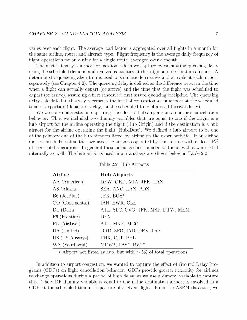
We were also interested in capturing the effect of hub airports on an airlines cancellationbehavior. Thus we included two dummy variables that are equal to one if the origin is ahub airport for the airline operating the flight (Hub Origin) and if the destination is a hubairport for the airline operating the flight (Hub Dest). We defined a hub airport to be oneof the primary one of the hub airports listed by airline on their own website. If an airlinedid not list hubs online then we used the airports operated by that airline with at least 5%of their total operations. In general these airports corresponded to the ones that were listedinternally as well. The hub airports used in our analysis are shown below in Table 2.2.

Table 2.2: Hub Airports

Airline Hub Airports

AA (American) DFW, ORD, MIA, JFK, LAX

AS (Alaska) SEA, ANC, LAX, PDX

B6 (JetBlue) JFK, BOS*

CO (Continental) IAH, EWR, CLE

DL (Delta) ATL, SLC, CVG, JFK, MSP, DTW, MEM

F9 (Frontier) DEN

FL (AirTran) ATL, MKE, MCO

UA (United) ORD, SFO, IAD, DEN, LAX

US (US Airways) PHX, CLT, PHL

WN (Southwest) MDW*, LAS*, BWI*

∗ Airport not listed as hub, but with > 5% of total operations

In addition to airport congestion, we wanted to capture the effect of Ground Delay Pro-grams (GDPs) on flight cancellation behavior. GDPs provide greater flexibility for airlinesto change operations during a period of high delay, so we use a dummy variable to capturethis. The GDP dummy variable is equal to one if the destination airport is involved in aGDP at the scheduled time of departure of a given flight. From the ASPM database, we


have information regarding the number of Expected Departure Clearance Time (EDCT)flights that are scheduled to arrive at a destination airport for a particular quarter-hourtime window. For a particular flight, we set the GDP variable equal to one if the destinationairport has a non-zero number of EDCT flights scheduled for arrival during the quarter hourthat corresponds to the flights scheduled departure time. We use the departure time hererather than arrival time because we are trying to capture the conditions at the destinationairport at the scheduled departure time. This time does not necessarily correspond to thetime that the cancellation decision is made or the time in which the EDCT flight informationis available to the airline (which is often much earlier), but since we do not know specificinformation about each EDCT flight we use this time in our analysis as a proxy for thecancellation decision time.

We are also interested in time-of-day effects. At the beginning of the day, airlines havemore resources available to handle flight disruptions. Cancellations affect flight operationslater in the day, since aircraft, passengers, and crew need to be changed from their originalschedule and flight delays build up throughout the day as small disturbances are propagatedthroughout the network. In addition, later flights have less flexibility for rescheduling pas-sengers than earlier flights, while cancelling them has less impact on flight legs downstream.

We used a simple four level categorical variable based on the local departure time for agiven flight. We divided the day into the following categories: (0300-0900, 0900-1500, 1500-2100, and 2100-0300). A dummy variable for each period was defined, with the 0300-0900category set to zero as a base for comparison.

Distance effects are likely important as well. Longer flights must be cancelled well inadvance of arrival time, so airlines do not have as much information about conditions at thedestination for longer flights compared to shorter flights. Longer flights are also less frequentand larger, but since we are already capturing those effects explicitly using other variables,we will capture any distance effects that are independent of these other effects. We usefive categories for distance, with the following ranges: 0-500 mi, 500-750 mi, 750-1000 mi,1000-1500 mi, and 1500 mi or greater). A dummy variable is used for each category withthe exception of the 500-750 mi category, which is set to zero as a base for comparison.

As mentioned earlier, one of the primary drivers of cancellations is weather. Thus, wecapture weather at both the origin and destination through several different variables. Theweather effects we measure are visibility, temperature, and wind speed, as well as indicatorsfor the presence of Instrument Meteorological Conditions (IMC), Rain, Thunderstorms, andSnow. We record the weather at the origin airport at the scheduled time of departure andat the destination airport at the scheduled time of arrival.

Lastly, we wanted to capture airline heterogeneity through fixed effects for each airline.Thus, we have 11 dummy variables in total, with Mesa Airlines low-cost Hawaiian carrier,go!Airlines arbitrarily chosen as the base. We also combined the regional affiliate flights withthe mainline carrier and designated a dummy variable that is equal to one if the flight isnot a mainline flight. For instance, if the flight is listed as a United flight, but operated byany of the regional affiliates under the United Express designation, then our regional carrierdummy will be set to 1 and the airline dummy for United will be set to 1 as well. A list of


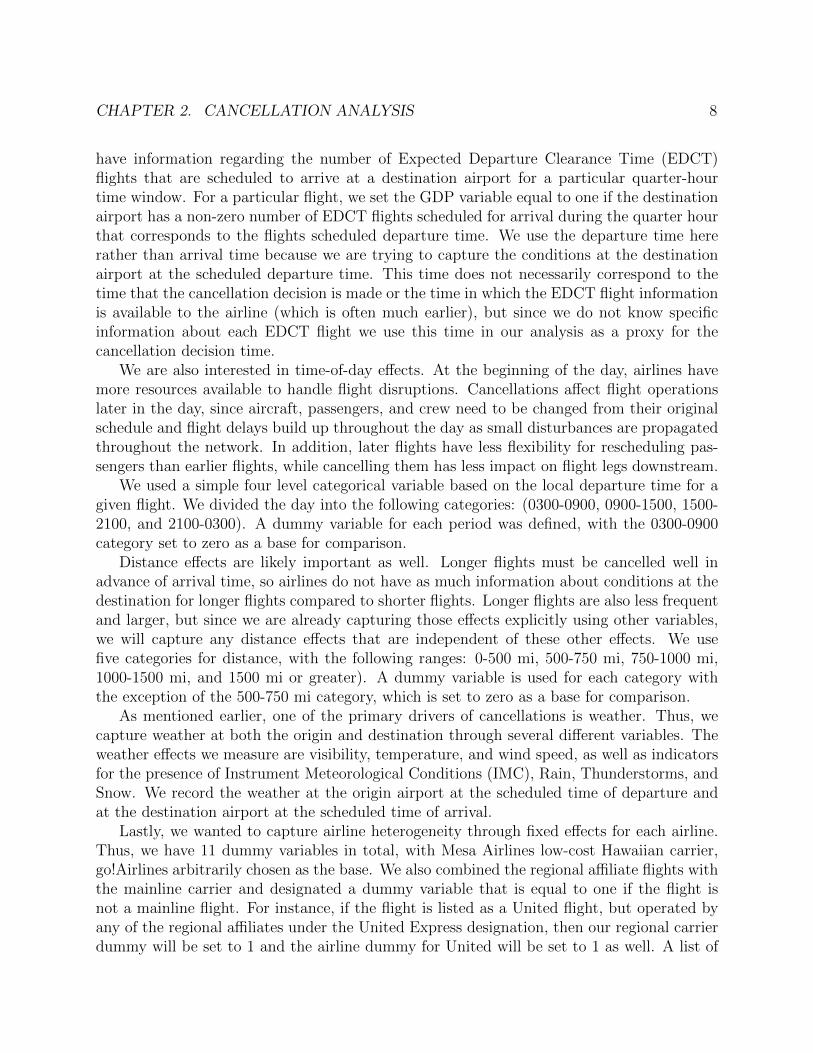
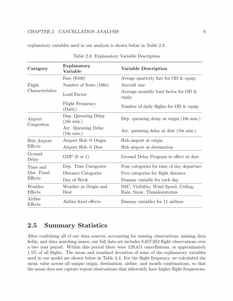
explanatory variables used in our analysis is shown below in Table 2.3.

Table 2.3: Explanatory Variable Description

CategoryExplanatoryVariable

Variable Description

FlightCharacteristics

Fare ($100) Aveage quarterly fare for OD & equip

Number of Seats (100s) Aircraft size

Load FactorAverage monthly load factor for OD &equip

Flight Frequency(Daily)

Number of daily flights for OD & equip

AirportCongestion

Dep. Queueing Delay(10s min.)

Dep. queueing delay at origin (10s min.)

Arr. Queueing Delay(10s min.)

Arr. queueing delay at dest (10s min.)

Hub AirportEffects

Airport Hub @ Origin Hub airport at origin

Airport Hub @ Dest Hub airport at destination

GroundDelay

GDP (0 or 1) Ground Delay Program in effect at dest

Time andDist. FixedEffects

Dep. Time Categories Four categories for time of day departure

Distance Categories Five categories for flight distance

Day of Week Dummy variable for each day

WeatherEffects

Weather at Origin andDest

IMC, Visibility, Wind Speed, Ceiling,Rain, Snow, Thundesrstorms

AirlineEffects

Airline fixed effects Dummy variables for 11 airlines

2.5 Summary Statistics

After combining all of our data sources, accounting for missing observations, missing datafields, and data matching issues, our full data set includes 8,857,952 flight observations overa two year period. Within this period there were 129,415 cancellations, or approximately1.5% of all flights. The mean and standard deviation of some of the explanatory variablesused in our model are shown below in Table 2.4. For the flight frequency, we calculated themean value across all unique origin, destination, airline, and month combinations, so thatthe mean does not capture repeat observations that inherently have higher flight frequencies.


Table 2.4: Variable Summary Statistics

Variable Mean Std. Dev.

Avg. Fare ($) 183.69 63.62

Number of Seats 129.37 40.6

Load Factor 0.8 0.1

Daily Flights 3.06 2.73

Dep. Queueing Delay (min.) 2.99 1.89

Arr. Queueing Delay (min.) 2.43 1.96

Hub Origin 0.31 0.46

Hub Destination 0.31 0.46

Ground Delay Program 0.04 0.2

Distance (<500 mi) 0.32 0.47

Distance (750-1000 mi) 0.17 0.38

Distance (1000-1500 mi) 0.16 0.37

Distance (>1500 mi) 0.15 0.35

Dep. Time (9:00-15:00) 0.05 0.09

Dep. Time (15:00-21:00) 0.38 0.48

Dep. Time (21:00-3:00) 0.21 0.41

Regional Carrier 0.19 0.39

Some things to note are the average queueing delay of around 3 minutes for departuresand 2.4 minutes for arrivals, and the 4% of flights that are involved in a GDP. The averagenumber of flights per day between a given origin and destination for a given airline is 3.1.31% of flights are departing from a hub, and 31% are arriving at a hub and almost 20% of allflights are operated by a regional carrier. The summary statistics (mean and std. deviation)for the weather effects used in our model are shown below in Table 2.5.

The mean value and standard deviation is shown for each variable. For the indicatorvariables (with a 0 or 1 value), the mean is simply the percentage of flights with that weathercondition. For instance, 14% of flights faced IMC conditions at the destination, and 1% offlights had snow at the destination at the time of scheduled departure. The average visibilitywas 9 miles, with a significant standard deviation (1.9 mi.), and the average wind speed was8.8 mph. Visibility ranged from 0 to 10 miles, with 84% of the observations having a visibilityof 10 miles. Wind speed ranged from 0 to 47 mph, with 90% of observations having a windspeed of less than 12 mph.

The percentage of flights cancelled for each airline in our sample is shown in Table 2.6,along with the percentage of flights from our sample operated by each airline and the totalnumber of cancellations during our sample period.


Table 2.5: Weather Summary Statistics

Variable Mean Std. Dev.

IMC Dest (0 or 1) 0.14 0.35

Temp Dest (deg F) 63.24 19.04

Vis Dest (mi) 9.33 1.9

WindSpd Dest (mph) 8.85 5.57

IMC Origin (0 or 1) 0.14 0.35

Temp Origin (deg F) 63.23 19.06

Vis Origin (mi.) 9.31 1.92

WindSpd Origin (mph) 8.82 5.55

Dest Rain (0 or 1) 0.06 0.23

Dest Snow (0 or 1) 0.01 0.12

Dest TStorm (0 or 1) 0.01 0.08

Origin Rain (0 or 1) 0.06 0.23

Origin Snow (0 or 1) 0.01 0.12

Origin TStorm (0 or 1) 0.01 0.08

There is large variation in cancellation percentages across airlines in our sample, rangingfrom Alaska Airlines that only cancelled 0.3% of its flights during the two-year period ofinterest, to American Airlines, which cancelled 2.4% of its flights. We have clear hypothesesabout how many of the flight characteristics in the model should affect the likelihood ofcancellation. Larger and fuller flights should be less likely to be cancelled in order to minimizethe cost due to rescheduling passengers. Higher fare routes should be cancelled less frequentlythan lower fare routes because the airlines are seeking to maximize profits. Routes withhigher fares are associated with the presence of high-value customers that represent a majorsource of revenue for the airline. Based on our discussions with airline employees, the airlinestry to minimize the inconvenience of these passengers by cancelling their flights less thanother flights with lower-value customers. High flight frequency between two airports allowsfor easier rebooking of passengers, so these flights should be more likely to be cancelledthan flights with low frequency. It is hypothesized that airlines seek to minimize their ownnetwork disruption through propagated delays, and thus flights into and out of hubs shouldbe less likely to be cancelled than other flights. Poor weather makes cancellations morelikely than fair weather. Airport capacities are reduced in times of poor weather, which canlead to large delays and cancellations. Lastly, congestion in the form of flight delays shouldmake cancellations more likely. These hypotheses, summarized below in Table 2.7, will bereferenced when discussing the results from the initial model.


Table 2.6: Airline Summary Statistics

Airline Cancellation % % of Flights Cancellations

DL (Delta) 1.80% 20% 31,889

UA (United) 1.50% 10% 13,287

US (US Airways) 1.40% 10% 12,401

AA (American) 2.40% 15% 31,889

CO (Continental) 1.40% 9% 11,161

WN (Southwest) 0.90% 22% 17,539

B6 (JetBlue) 1.50% 4% 5,315

F9 (Frontier) 0.40% 2% 709

FL (Air Tran) 1.00% 5% 4,429

AS (Alaska) 0.30% 3% 797

Overall 1.48% 100% 129,416

2.6 Estimation Results

The large amount of data in our sample prohibited us from estimating a single model forall flights across the two year time span. Thus, we created a simple random sample that isapproximately 33% of the size of the full sample by selecting each flight for inclusion in thesub-sample with equal probability. The resulting subsample accounted for 3 million flights.The model estimates are shown below in Table 2.8 and Table 2.9.

As shown in Table 2.9, above, the vast majority of the variables are significant. With oneexception, results match our expectations. Fare appears to have a positive and significanteffect, which is contrary to our hypothesis. The estimated coefficients on other flight charac-teristic variables are consistent with our expectations. Load factor has a negative and largesign. Higher load factors make a flight much less likely to be cancelled. Similarly, aircraftsize has a negative effect as well. Departure time of day shows an increasing likelihood ofcancellation as the day progresses. The baseline departure time category is 3:00 9:00, so thesigns of the coefficients of the other categories are measured relative to the baseline category.There is a small negative sign for 9:00 15:00 and a small positive sign for 15:00 21:00.The coefficient for the last group, 21:00 3:00 is much larger than the other coefficients andpositive. This indicates that late night flights are more likely to be cancelled than earlierflights. We expect later flights to be cancelled more than earlier flights at least partiallydue to higher delays that build up over the course of the day. Although we are capturingqueueing delays explicitly, these do not reflect the cumulative effect of earlier delays on aflight.

The distance effects generally match our expectations. The baseline category is the500-750 mile group, so the coefficients are interpreted with respect to that category. The


Table 2.7: Cancellation Hypotheses

Flight Cancellation Hypotheses

Flight Characteristic TrendImpact on CancellationLikelihood

Larger aircraft (vs smaller aircraft) Less likely

High load factor (vs low load factor) Less likely

Route with higher average fare (vs lower average fare) Less Likely

Route with high flight frequency (vs low frequency) More likely

Flight is into or out of airline hub Less likely

Flights with poor weather at origin or destination More likely

Flights with more queueing delay at origin or destination More likely

Flight with GDP at destination More likely

Flight operated by regional carrier More likely

Longer flights (vs shorter flights) Less likely

Evening departure times (vs morning departure times) More likely

distance effect decreases roughly monotonically with distance. Thus we see that, in general,longer flights are less likely to be cancelled than shorter flights, even when accounting forthe effects of aircraft size, load factor, and frequency separately. This is consistent withour expectations and conversations with flight dispatchers. Airlines can wait longer to makecancellation decisions for shorter flights so that they have better information about conditionsat the destination. Thus they tend to allow longer flights to proceed on the assumption thatconditions at the destination at the time of arrival will be fairly normal. This behavioris further encouraged under GDPs when longer flights are often exempted from grounddelays. Flight frequency is positive and significant, which also matches our expectations.We would think that the more flights that are offered by an airline on a particular routemakes accommodating passenger routing changes easier when a cancellation is necessary.Thus, a flight on a route with higher frequency is most likely to be cancelled than a flighton a route with lower frequency, all else equal. These effects together illustrate the tradeoffsmade by airlines to minimize the disruption of passengers.

Both of the queueing delay variables, which represent the level of congestion at the originand destination airport, are statistically significant and positive, with similar magnitudes.This indicates that larger queueing delays, caused by an imbalance between demand andcapacity, highly influence cancellations. We suspected that there was a non-linear effect ofqueueing delay on cancellation utility, so we included the square of departure and arrivaldelay as well. These two coefficients are both negative and significant, which suggests thatthere is a diminishing marginal effect on cancellation utility as the queueing delays become


Table 2.8: Logit Estimation Results 1

Variable Est.Std.Err.

Variable Est.Std.Err.

ASC(Cancel) -2.422 ** 0.118 IMCDest -0.025 0.016

Fare($100) 0.071 ** 0.011 TempDest (10s deg F) -0.012 ** 0.004

DepTime(9:00-15:00) -0.064 ** 0.014 VisDest (mi.) -0.073 ** 0.003

DepTime(15:00-21:00) 0.041 ** 0.014 WindDest (mph) 0.019 ** 0.001

DepTime(21:00-3:00) 0.159 ** 0.041 IMCOrigin 0.031 0.016

Miles<500 -0.004 0.014 TempOrigin (10s deg F) -0.029 ** 0.004

Miles750-1000 -0.137 ** 0.018 VisOrigin (mi.) -0.097 ** 0.003

Miles1000-1500 -0.105 ** 0.02 WindOrigin (mph) 0.03 ** 0.001

Miles1500more -0.303 ** 0.026 Hub Origin -0.245 ** 0.017

Num.Seats(100) -0.276 ** 0.037 Hub Dest -0.086 ** 0.017

LoadFactor -2.142 ** 0.051 GDP 0.359 ** 0.022

Flight Frequency(flight/day)

0.039 ** 0.002 Dest Rain 0.047 * 0.019

Dep. Delay (10s min) 0.302 ** 0.009 Dest Snow 0.93 ** 0.024

Arr. Delay (10s min) 0.319 ** 0.01 Dest TStorm 0.867 ** 0.039

Dep. Delay Squared(100s min2)

-0.014 ** 0.001 Origin Rain 0.2 ** 0.019

Arr. Delay Squared(100s min2)

-0.014 ** 0.001 Origin Snow 0.982 ** 0.024

Sunday -0.149 ** 0.019 Origin TStorm 0.949 ** 0.039

Monday -0.218 ** 0.019 Regional Carrier 0.124 ** 0.036

Tuesday -0.068 ** 0.018

Thursday -0.08 ** 0.018

Friday -0.149 ** 0.018 ** Significant at 1% level

Saturday -0.26 ** 0.021 * Significant at 5% level

very large.Next, we consider the day-of-week effects. Wednesday is set to zero as a baseline for

comparison. The results suggest that flights on weekend days are less likely to be cancelledthan flights in the middle of the week. Based on conversations with flight dispatchers, aircraftmaintenance is often scheduled for the middle of the week, which makes aircraft substitutionsmore difficult in the event of a mechanical issue. This could be one reason for this trend in


Table 2.9: Logit Estimation Results 2

Variable EstimateStd.Err.

DL (Delta) 1.132 ** 0.096

UA (United) 1.156 ** 0.097

US (US Airways) 0.914 ** 0.096

AA (American) 1.423 ** 0.096

CO (Continental) 0.764 ** 0.098

WN (Southwest) 0.82 ** 0.095

B6 (JetBlue) 1.199 ** 0.098

F9 (Frontier) 0.262 * 0.117

FL (Air Tran) 0.625 ** 0.1

AS (Alaska) -0.01 0.115

cancellations throughout the week.The weather effects are mostly significant and consistent with our expectations. The

only non-significant weather variables are the IMC variables, which indicate that we areexplicitly capturing all of the factors contributing to IMC conditions directly in the otherweather variables. Higher temperatures are generally an indication of better weather, andthese result in flights being less likely to be cancelled. High winds and low visibility increasethe chances of a flight being cancelled. We see a similar effect of weather at both the originand destination. Recall that we measured the weather for the origin at the scheduled time ofdeparture and for the destination at the scheduled time of arrival. The cancellation decisionhas be made prior to departure, so there is inherently less certainty associated with theweather conditions at the destination. It appears that forecasts are reliable enough at thetime of these decisions to overcome this.

The other weather variables were entered as indicators, taking a value of one if thecondition was present. The conditions we measured were rain, snow, and thunderstorms atthe origin and destination. Not surprisingly, the presence of snow and thunderstorms increasethe chance of cancellation more than rain. To gauge the magnitude of the effect of snowand thunderstorms on the cancellation likelihood, note that the presence of thunderstormsat the origin is equivalent to almost 30 mph winds, while the presence of snow has an evenstronger effect. Snow and thunderstorm have impacts of roughly equal magnitude whetherthey are at the origin or destination, similar to what we saw for visibility and wind.

Next we look at the hub variables. These are indicator variables that are equal to one ifthe flight departs from a hub airport of the airline operating the flight (HubOrigin) or arrivesat a hub airport of the airline operating the flight (HubDest). Both of these coefficients arenegative and significant, with the origin variable having a larger magnitude. These results


Figure 2.1: Airline Fixed Effects and Average Cancellation Pct.

suggest that airlines do not like to cancel flights into or out of their hub airports. Theseflights are important to airlines due to the large number of connecting passengers at hubairports, so this result is not surprising. This also may explain why the HubOrigin effectis the stronger one, since a cancellation of a flight from a hub strands passengers at theconnecting hub, rather than their origin or destination.

Now we will consider the airline fixed effects, including the dummy variable for regionalcarriers. We see that the regional carrier dummy is positive and significant. Regional carrierflights are more likely to be cancelled than mainline flights operated by the same airline,all else equal. This is consistent with what weve seen in practice. Regional carrier flightstypically have other characteristics that are favorable for flight cancellations (i.e. short flightdistance, smaller planes, operating out of hubs), so the cancellation effect for these flights iseven stronger than what are suggested by the coefficient for the regional carriers. The airlinedummy variables (2.9) are all positive and significant, with the lone exception of AlaskaAirlines. Recall that the airline used as the base is the low-cost carrier of Mesa Airlines, go!Airlines. All the coefficients can be interpreted relative to this base carrier. To better inferthe meaning of the coefficients, we present a scatter plot of the overall cancellation percentagefor the airline on the x-axis and the coefficient fixed effect for the airline on the y-axis. Thisallows us to observe airlines proclivity to cancel relative to others when controlling for theproperties of the flights the airline operates, as compared to the raw cancellation percentages.This plot is shown below in 2.1.

From Figure 2.1, we can see that the fixed effect coefficients and cancellation percentageare highly correlated. We can conclude from this that there are large differences in thecancellation rates across airlines and the differences are not caused by differences in the


characteristics of the flights, airports, and operating conditions. Some airlines just cancelmore than others. The former group consists largely of network, legacy carriers and thelatter of low cost carriers. The one exception to this pattern is Jet Blue (B6), which hasabout the same cancellation proclivity as United, Delta, and US Airways.

We tried various model specifications, including one with airport fixed effects. Specifically,we used dummy variables for flights with an origin or destination at the 16 largest airports.The improvement in model fit was very small compared to the improvement gained by theairline fixed effects. Thus, for our final model we use only airline fixed effects and leave outany airport fixed effects.

We can quantify the effects for each variable by calculating the odds ratio for a givenchange in a parameter. We define the odds of cancellation as the ratio of the probability ofcancelling a flight and the probability of not cancelling a flight:

Odds =pcancel

1− pcancel(2.3)

The cancellation probabilities have a closed form solution, as shown in Equation 2.2. Wecan use the analytical expression from that equation to re-write the odds ratio as follows:

Odds =

eVcancel

1−eVcancel

1− eVcancel

1−eVcancel

=

eVcancel

1−eVcancel1

1+eVcancel

= eVcancel = e∑j βjxcancel,j (2.4)

The odds ratio is simply the ratio of the odds for two different sets of explanatoryvariables. For example, we can increase the value of one explanatory variable by 1 unitand calculate the odds ratio based on the increase. For this example, we will assume thatxcancel,j is increased by 1 unit:

OR1 =e∑j βjxcancel,j+β1

e∑j βjxcancel,j

=e∑j βjxcancel,je

β1

e∑j βjxcancel,j

= eβ1 (2.5)

The odds ratio for a one unit change in an explanatory variable is simply the exponentialfunction of the coefficient for that explanatory variable. We can re-write the results of Table2.8 and Table 2.9 in terms of odds ratios for a unit change in the explanatory variables. Forsome of the explanatory variables, we present the odds ratio for a smaller than unit changein the variable, since a unit change would not represent changes that appear in our dataset.For example, a 1 unit change in load factor is the entire range for that variable. The oddsratios are presented below in Table 2.10.

The odds ratios presented in Table can give us a better sense for the magnitude of theimpact each explanatory variable has on the relative likelihood of cancelling a flight. Forexample, the odds of cancelling a given flight is only 76% that of cancelling a flight with 100fewer seats. Conversely, the odds of cancelling a flight are 1.32 times greater than those foran otherwise identical flight with 100 more seats (1/0.76 = 1.32). The magnitudes of theodds ratios for flight characteristics are much smaller than the magnitude for the odds ratios


for weather effects. Consider the odds ratio for the GDP variable, which indicates that theodds of cancelling a flight with a GDP at the destination airport are 1.43 times greater thanthe odds of cancelling an identical flight without a GDP at the destination airport. Clearlythe weather effects are very strong, especially considering many of them could happen atthe same times. For example, consider a flight with a GDP at the destination, and snow atboth the origin and destination. The combined odds ratio for these three conditions is theproduct of the three individual odds ratios, or 9.69. The odds of cancelling such a flight arenearly 10 times those of cancelling a similar flight without the presence of snow and a GDP.

2.7 Cancellation Predictions

We can use the results from the above cancellation model to predict cancellations. We usethe cancellation probability formula shown in Equation 2-2, and using our estimates fromTable 2.8 and Table 2.9, we can generate a cancellation probability for each flight basedon the observable characteristics. Flights that have characteristics favorable for increasedchances of cancellations, such as low load factor, small aircraft, short flights in bad weather,will have higher cancellation probabilities than flights with characteristics not favorablefor cancellation, such as large aircraft, high load factor, hub-to-hub flights in the morninghours on a good weather day. The coefficients above give us a qualitative sense for whichcharacteristics will lead to a higher or lower cancellation probability, but do not give usa sense for the magnitude of those cancellation probabilities. To illustrate the magnitudethat we are talking about here, we calculated the predicted cancellation probability for thesample of flights used in our analysis and plotted the cumulative probability distribution ofthe predicted cancellation probabilities. This plot is shown below in Figure 2.2.

The curve in Figure 2.2 represents the cumulative probability of the cancellation proba-bility defined by the x-axis. For example, the median cancellation probability for our sampleis just below 1%. The mean cancellation probability for our sample is 1.5%. The 90th per-centile of cancellation probabilities is less than 3%. The flights with a predicted cancellationprobability higher than this typically have a combination of favorable flight characteristicsfor cancellations and poor weather. We almost never see cancellation probabilities above20%, even when considering all of these effects.

2.8 Model Fit

So far we have interpreted the cancellation model coefficients in terms of their effect on apredicted cancellation probability, but we have not addressed how well the predicted cancel-lation probabilities match the cancellations that actually happened. We investigate this bypredicting the cancellation probabilities for all flights in our sample and aggregating themover a single day for a single airport. This will give us a total number of predicted flight


Table 2.10: Logit Model Odds Ratios

VariableUnitIncrease

OddsRatio

VariableUnitIncrease

OddsRatio

Fare($100) $100 1.07 IMCDest 1 0.97

DepTime(9:00-15:00) 1 0.94 TempDest 10 deg 0.99

DepTime(15:00-21:00) 1 1.04 VisDest 1 mi 0.93

DepTime(21:00-3:00) 1 1.17 WindDest 10 mph 1.21

Miles¡500 1 1 IMCOrigin 1 1.03

Miles750-1000 1 0.87 TempOrigin 10 deg 0.97

Miles1000-1500 1 0.9 VisOrigin 1 mi 0.91

Miles1500more 1 0.74 WindOrigin 10 mph 1.35

Num.Seats (100) 100 0.76 Hub Origin 1 0.78

LoadFactor 10% 0.81 Hub Dest 1 0.92

Flight Frequency(flight/day)

1 1.04 GDP 1 1.43

Departure Delay (min) 10 min 1.35 Dest Rain 1 1.05

Arrival Delay (min) 10 min 1.38 Dest Snow 1 2.54

Dep. Delay Squared(min2)

100 min2 0.986 Dest TStorm 1 2.38

Arr. Delay Squared(min2)

100 min2 0.986 Origin Rain 1 1.22

Sunday 1 0.86 Origin Snow 1 2.67

Monday 1 0.8 Origin TStorm 1 2.58

Tuesday 1 0.93 Regional Carrier 1 1.13

Thursday 1 0.92

Friday 1 0.86

Saturday 1 0.77

cancellations for a particular airport and a particular day. We can then compare this numberto the total actual number of cancellations on that same day.

Across all airports and all days, our model should give the exact number of cancelledflights. This is a result of us including an alternative-specific constant in the model specifi-cation. Doing this forces the actual percentage of flight cancellations to equal the predictedpercentage of flight cancellations. This does not have to be true across any subset of oursample, however, so we can use the comparison described above to determine how robust


Figure 2.2: CDF of Cancellation Probability for One Month Sample

the model is for cancellation predictions at a smaller level.The method of sample enumeration is used for predicting flights for a single day. The

following formula illustrates the technique:

Ci,t =n∑j=1

pjdt,i

The predicted number of cancellations on day t at airport i is given by Ci,t. The totalnumber of flights in our sample is given by n, each flight j of which has a predicted cancel-lation probability by pj. dt,i is a dummy variable, equal to 1 when the flight is on day t withdestination airport i, and 0 otherwise.

We will compare the predicted number of cancellations based on our model, Ci,t, withthe actual number of cancellations, Ci,t. For a destination airport i, each day t will be

represented by two numbers, (Ci,t, Ci,t). We can plot these points to compare the predictednumber to the actual number. If the model perfectly predicts the number of cancellationsfor a given destination airport-day, then all points will lie on the 45 degree line.

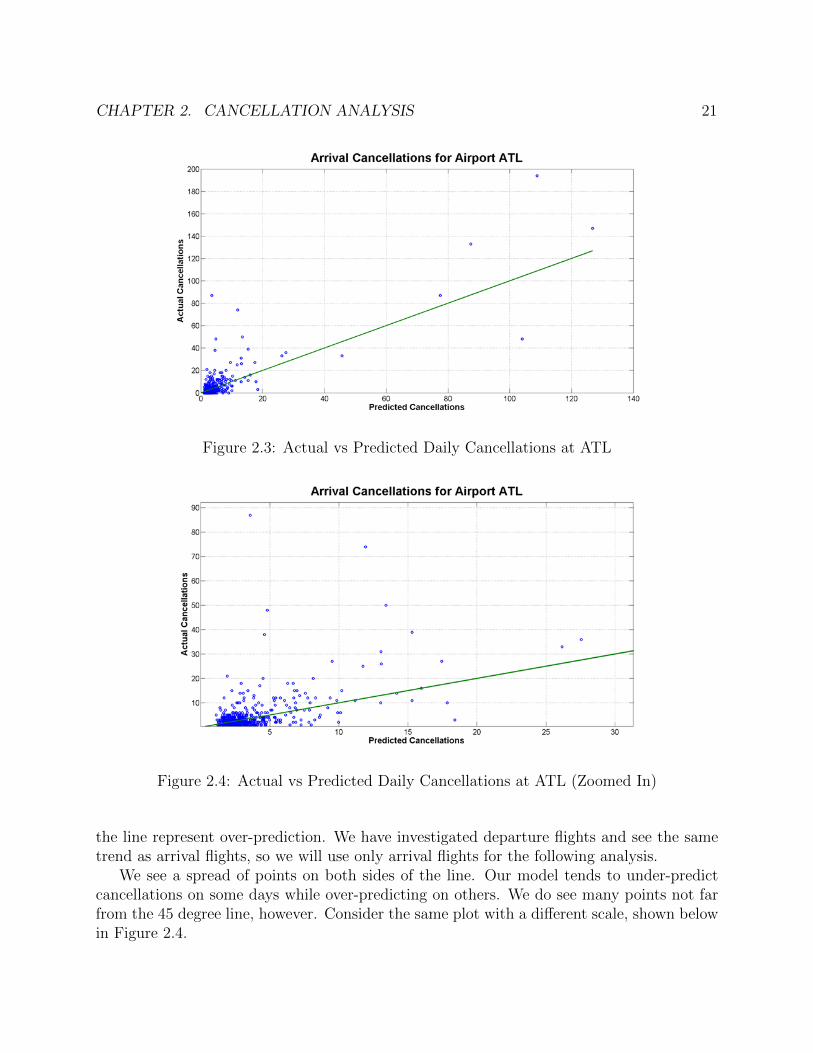
Consider an example of flights into ATL from our sample, shown below in Figure 2.3.On the x-axis we have the predicted number of cancellations and the y-axis the actualnumber of cancellations. The line shown is the 45 degree line, where the actual number ofcancellations equals the predicted number of cancellation. Each point shown is a day fromour sample. Points above this line represent cases of under-prediction, where the actualnumber of cancellations was more than the predicted number of cancellations. Points below


Figure 2.3: Actual vs Predicted Daily Cancellations at ATL

Figure 2.4: Actual vs Predicted Daily Cancellations at ATL (Zoomed In)

the line represent over-prediction. We have investigated departure flights and see the sametrend as arrival flights, so we will use only arrival flights for the following analysis.

We see a spread of points on both sides of the line. Our model tends to under-predictcancellations on some days while over-predicting on others. We do see many points not farfrom the 45 degree line, however. Consider the same plot with a different scale, shown belowin Figure 2.4.


Figure 2.5: Actual vs Predicted Daily Cancellations at BOS

Now we can clearly see a large cluster of days when both the actual and predictednumber of cancellations is less than 5. Beyond this some spread exists in both directions.These prediction results are similar at other airports. Consider the sample plot for BOS,shown in Figure 2.5, below.

Again, we can see there is a large cluster of flights around less than 5 cancellations,with some spread in both directions from the 45-degree line. From inspection it is hard todistinguish these results from those at ATL, however. At first glance, it might appear thatour model is not doing a good job predicting cancellations, since not many of the pointslie exactly along the 45 degree line. Some discrepancy is to be expected, however, sincecancellations are low probability events. Thus we need a more formal way of evaluating themodel fit than the naked eye.

As another form of model fit, we can compare the number of predicted cancellationsaggregated across all days for a given airport with the total number of actual cancellationsaggregated across all days for the same airport. A plot with many days of over-predictionand many days of under-prediction can cancel out and result in a total number of predictedcancellations similar to that which was observed. The number of predicted and actualcancellations for each airport is shown below in Table 2.11.

The airports with the closest number of predicted and actual cancellations are ATL, BOS,DFW, LGA, PHL, and SFO, each with less than 8% difference between the predicted andactual. The airports with the largest discrepancy between the actual number of cancellationsand the predicted number were EWR, IAD, IAH, JFK, and MSP, each with over 25%difference in the number of cancellations. Also since cancellations are rare events, one wouldexpect the standard errors of the predicted numbers to be approximately the square root ofthe predicted number generally between 25 and 50 for the airports listed. Clearly, in many


Table 2.11: Total Predicted and Actual Cancellations by Airport

Airport Actual Pred. % Diff. Airport Actual Pred. % Diff.

ATL 3032 2885 -4.80% LAS 585 711 21.60%

BOS 1988 1931 -2.90% LAX 1293 1411 9.20%

BWI 851 677 -20.50% LGA 2464 2507 1.80%

CLT 1167 983 -15.80% MCO 574 637 10.90%

DCA 1487 1211 -18.50% MDW 522 565 8.20%

DEN 878 1082 23.30% MIA 727 583 -19.90%

DFW 2092 2098 0.30% MSP 807 1022 26.60%

DTW 1063 1206 13.50% ORD 3629 3943 8.70%

EWR 1930 1445 -25.10% PHL 1123 1086 -3.30%

IAD 830 608 -26.70% PHX 1076 885 -17.80%

IAH 645 859 33.20% SAN 511 627 22.70%

JFK 1581 1183 -25.20% SFO 1128 1039 -7.90%

cases, the difference between predicted and observed cancellation numbers is well outsidethe ±2σ 95% confidence bounds derived from these standard errors.

To further investigate the distribution of daily cancellations, we can think of the numberof cancellations predicted by our model as the expected number for a given day. Even if thepredicted number, on average, matches the actual number, any number of realizations willshow a discrepancy between the two numbers. In particular, think about the days of veryhigh under-prediction shown in the plot for ATL in Figure 2-4. Considering that we arelooking at 730 airport-days, we might expect one or two of them to be very far away fromthe mean values predicted by our model, simply due to statistical fluctuations. We need todo something more than just inspect the plots of actual versus predicted cancellations inorder to tell how well the model predicts cancellations for single airport-days.

We can use a statistical test to determine how well the predicted distribution of cancel-lations matches the actual distribution of cancellations. We will assume that the number ofcancellations for a given day follows a Poisson distribution with a mean value equal to thenumber predicted by our model. Therefore, for a single day, we can define the probability ofobserving a specific number of cancellations by the following equation:

P (Ci,t = k) =e−λi,tλki,t

k!(2.6)

where: Ci,t = number of cancellations at airport i on day t and

λi = predicted number of cancellations at airport i on day t, equal to Ci,tSimilarly, the probability of observing less than or equal to some specific number of

cancellations is shown in the following formula:


Figure 2.6: Empirical CDF of Cumulative Cancellation Probabilities at ATL

P (Ci,t ≤ K) =K∑k=0

eλi,tλki,tk!

(2.7)

We will calculate, for each airport-day, the probability of observing less than or equal tothe number of cancellations actually observed for that airport-day, using the formula above.If the model correctly predicts the distribution of the number of cancellations, then we wouldexpect the calculated probability to be approximately equal to the empirical probabilitybased on the number of days in the data set. For example, we expect roughly 50% of thedays to have a probability of less than or equal to 50% based on equation –. We can comparethese two distributions for a given airport by plotting the empirical CDF of the cumulativeprobabilities calculated using equation –, for all days in our sample. The result for Atlantais shown below in Figure 2.6.

The empirical CDF of cumulative probability calculated from equation – is shown in theblue curve. The red line is the 45-degree line represents the empirical CDF of the observedcancellations for each day. The probability calculated for each airport-day using equation –is sorted in ascending order, then each day is assigned a cumulative probability defined asfollows:

Pn =N∑n=1

n

N(2.8)

Where n is the number of the day in the ordered sample, and N is the total number ofdays. Thus, the empirical CDF of these probabilities is simply the 45 degree line. We use


Figure 2.7: Empirical CDF of Cumulative Cancellation Probabilities at BOS

this as a basis of comparison for the empirical CDF of the cumulative probabilities calculatedusing equation –. The closer the blue curve is to the red line, the better the model does inpredicting the distribution of the number of cancellations for individual airport-days.

As seen in Figure 2.6, the blue curve oscillates around the red line, being above the linefor probabilities below 0.7 and below the line for higher probabilities. In the former case,a larger fraction of days has a calculated probability below a certain value than the modelpredicts. For example, about 60% of days have a probability below 50%. Put another way,for 60% of days, the number of cancellations, based on the cancellation model and equation–, is on the low side of what might be expected. In contrast, only about 84% of days havea calculated probability below 90%. Conversely 16% of days have numbers of cancellationsthat, according to the model, should be exceeded 10% of the time. Similarly, on roughly 4%of days, the number of cancellations is almost impossibly large according to the model, sincethe calculated cumulative probability is well above 99%. These days are represented by thenearly vertical part of the curve on the right of Figure 2.6.

Another way to interpret Figure 2-6 2.6 is to compare the slopes of the blue and redcurves. When the slope of the blue curve over some region of the CDF is steeper than45 degrees, there are more observed days in this region than the probability model wouldsuggest, and vice versa. It is evident that there are more days with cancellations in the 0-0.2range of the predicted distribution than expected, fewer days in the 0.4-0.9 range, and thenmany more days on the far right tail of the distribution.

A similar plot for BOS appears in Figure 2.7. The blue curve tracks the red curvemore closely in this case, although even here we see a vertical segment of the blue curveon the right, indicating days in which cancellations on the far right tail of the distributionare overrepresented. Consider IAD, shown below in Figure 2.8. In this case there are many


Figure 2.8: Empirical CDF of Cumulative Cancellation Probabilities at IAD

fewer days with realized cancellations on the left tails of the distributions up to a cumulativeprobability of about 0.4, more days in the range between 0.4 and 0.6, and again more dayson the right tail starting at about 0.85.

Some variation between the modeled and observed distributions for the number of can-cellations will result from random fluctuations. It is therefore of interest to formally testthe statistical significance of the observed differences. The Kolmogorov-Smirnov Test (KSTest) is a well-known statistical test that is used for comparing whether two datasets comefrom the same distribution. In our case, we are comparing the blue curve and the red curve.Conceptually, the KS Test is very easy to perform. The test statistic is simply the largestvertical difference between the two curves at a single x value. The test statistic is then usedto calculate a p-value, by which the null hypothesis (the two datasets come from the samedistribution) is either reject or not rejected. Mathematically, the test statistic is calculatedas follows:

Dn = supx|Fn(x)− F (x)| (2.9)

where supx is the supremum set of distances between the two curves, Fn(x) is the empiricalcumulative distribution function of the data, and F (x) is the cumulative distribution functionof the red curve, which follows a uniform distribution between 0 and 1. The test statistic,Dn follows the Kolmogorov distribution and from this we can calculate a p-value, whichrepresents the probability of observing the distributions we saw given the assumption thatthey both come from the same underlying distribution. Thus, for the statistical test tosuggest that the distributions are the same, it would yield a high p-value, indicating thatwe cannot reject the null hypothesis that the two distributions are the same. The p-values


calculated for the largest airports in our sample are shown below in Table 2.12. Along withthe p-values, we report the test statistic calculated using Equation 2.9.

Table 2.12: KS Test P-Values for Logit Model

Airport P-val Dn Airport P-val Dn

ATL 0.00053 0.1 LAS 0 0.25

BOS 0.0405* 0.07 LAX 0.0114* 0.08

BWI 0 0.26 LGA 0.0015 0.1

CLT 0 0.19 MCO 0 0.28

DCA 0 0.17 MDW 0 0.32

DEN 0 0.12 MIA 0 0.34

DFW 0 0.13 MSP 0 0.17

DTW 0.00053 0.1 ORD 0 0.12

EWR 0 0.14 PHL 0 0.23

IAD 0 0.33 PHX 0 0.25

IAH 0 0.16 SAN 0 0.28

JFK 0 0.13 SFO 0 0.2

* Not significant at 1% level

We can see from Table 2.12 that the p-values are very small for the most part. The p-values that were written with no significant digits (as 0) were so small that we can considerthem to be zero. There are only two airports where we cannot reject the null hypothesis ata 1% level of significance: BOS and LAX. The rest of the airports result in a distributionthat is different enough from what we would expect that we can reject the null hypothesiswith a very high level of confidence. BOS and LAX both had a small percentage differencebetween the total predicted and total actual cancellations (see Table 2.11), but were not thetwo best airports for this metric.

These results are not surprising, since they are testing a hypothesis that is very strong:that cancellations are independent events whose probabilities can be predicted by a modelthat applies to all airports in all situations. Our results show that this is clearly not thecase. Beyond this, we can consider the test statistic shown as Dn in Table 2.12, above, to bea metric for how well the model does at predicting cancellations for each airport. Althoughwe may not be able to statistically validate the predictions for most of these airports, wecan distinguish between them in terms of model fit. For instance, ATL and LGA havea much better fit than PHL, although the total number of cancellations predicted at thethree airports is roughly the same compared to the actual number, from Table2.11. Theseresults help identify the airports where the hypothesis is closer to and further from the truth,although it is not completely valid for any airport.


In a similar vein, hypothesis tests aside, our cancellation model is fairly good at predict-ing the number of cancellations by airport. In many cases it predicts the distribution ofcancellations by airport-day reasonably well. The airport-day results show that the hypoth-esis that cancellations are independent events whose probabilities can be calculated from theestimated model must be rejected, but they also show that the model predictions, for mostairports and most days, are reasonably accurate.

29

Chapter 3

Cancellation Model Extensions

This chapter explores additional models that expand upon the work shown in Chapter 2.We will assume the airlines are the decision-makers regarding flight cancellations, so wefirst investigate airline-specific choice models of the same form used in Chapter 2. Wealso suspect the assumption of iid error terms in the multinomial logit model is a bit toorestrictive. Thus, we relax this assumption and estimate a mixed logit model with a randomerror term. Finally, we anticipate different cancellation behavior during times of adverseweather, so we estimate a latent class model with two classes that capture the effect of flightcharacteristics on cancellation likelihood during times of calm and inclement weather.

3.1 Airline-Specific Models

Given the large amount of heterogeneity observed due to the airline fixed effects in the binarylogit model presented in Table 2.9 , we estimated separate models for each airline. In additionto the cancellation rates being different across airlines, we suspect that the coefficients forthe flight characteristics differ across airlines as well. We used the same sample as beforeand estimated a binary logit model with the same specification as that for the aggregatemodel. The results are presented below in Table 3.1 and Table 3.2. Due to the quantityof estimation results, we only present the estimate values themselves, and note statisticalsignificance at the 5% level with a bolded estimate. Table 3.3 and Table 3.4 present theairline-specific results in the form of odds ratios for each coefficient.

Some variables have large differences across airlines, such as the hub fixed effects. Unitedhas positive coefficients for both origin and destination, while the rest of the airlines ei-ther have either negative coefficients for both or a mixture of not significant and negativecoefficients. Fare, departure time, and day of week are also quite varied across airlines.

There is generally more consistency across coefficients for the legacy carriers than the lowcost carriers. For instance, the distance effects are roughly constant for all legacy carrierslonger flights are less likely to be cancelled. We see that for the low cost carriers, there arefew airlines with a clear trend at all for the distance effects. Load factor is negative and

CHAPTER 3. CANCELLATION MODEL EXTENSIONS 30

significant for all legacy carriers, but positive for JetBlue and not significant for Frontier.The most consistent variables across all airlines are queueing delay, snow, visibility, andwinds.

The regional carrier dummy variable is positive and significant for United, Continental,and American, not significant for US Airways and Alaska, and negative and significant forDelta and AirTran. Although we saw this variable enter as positive and significant in theaggregate model, we see different effects for each airline individually. We would suspectthe regional carrier effect to be positive and significant, so it is interesting that we find anegative and significant estimate for Delta and AirTran. Based on the odds ratios, Delta isalmost twice as likely to cancel a mainline flight as a regional carrier flight, while Americanand Continental are almost twice and three times as likely, respectively, to cancel a regionalcarrier flight.

Overall we see some consistent effects across all airlines, but in general there is significantheterogeneity with respect to many of the explanatory variables.

CHAPTER 3. CANCELLATION MODEL EXTENSIONS 31T

able

3.1:

Air

line-

Sp

ecifi

cL

ogit

Est

imat

es1

Delta

United

US

Airways

Am

erican

Continenta

lSouth

west

JetB

lue

Frontier

AirTran

Alask

a

AS

C(C

an

cel)

-0.553

-2.288

-2.088

-3.162

-2.884

-0.1

22

-0.8

21

-4.93

1.1

16

0.5

84

Fare

($100)

-0.0

38

0.0

42

0.231

0.34

-0.0

10.188

-0.296

0.0

40.193

0.142

Dep

Tim

e(9:0

0-1

5:0

0)

-0.169

-0.0

61

0.0

59

-0.12

-0.0

82

0.154

0.1

3-0

.195

0.0

01

-0.0

51

Dep

Tim

e(15:0

0-2

1:0

0)

-0.069

0.0

47

-0.0

02

0.0

14

0.219

0.183

0.306

0.3

42

0.1

06

-0.1

18

Dep

Tim

e(21:0

0-3

:00)

-0.0

83

0.0

57

0.268

-0.0

16

0.1

35

-0.0

01

0.829

1.434

0.453

-0.0

97

Miles

¡500

0.0

05

-0.0

17

0.0

36

-0.0

51

0.0

18

-0.0

46

-0.233

-0.1

86

-0.0

26

-0.914

Miles

750-1

000

0.1

-0.492

-0.0

89

-0.425

0.0

11

0.1

12

0.0

88

-0.397

-0.0

68

-0.4

13

Miles

1000-1

500

-0.23

-0.666

-0.31

-0.364

0.0

31

0.266

0.307

-0.728

-0.3

15

-0.3

69

Miles

1500m

ore

-0.327

-0.728

-0.457

-0.835

-0.252

0.351

0.1

22

-0.763

-0.615

-0.2

83

Nu

m.S

eats

(100s)

-0.572

-0.352

-0.1

76

0.387

0.352

0.0

27

-0.87

1.0

51

-2.16

-0.8

81

Load

Fact

or

-2.11

-0.9

98

-1.432

-1.434

-1.829

-4.478

0.905

0.4

37

-2.886

-3.292

FlightF

requ

ency

(flig

ht/

day)

0.008

0.02

0.029

-0.011

-0.061

0.132

0.0

29

-0.0

45

0.031

0.086

Dep

.D

elay

(10s

min

)0.351

0.249

0.256

0.365

0.473

0.337

0.272

-0.0

34

0.292

0.2

26

Arr

.D

elay

(10s

min

)0.33

0.318

0.239

0.313

0.45

0.324

0.279

0.517

0.427

0.3

19

Dep

.D

elay

Squ

are

d(1

00s

min

2)

-0.02

-0.01

-0.009

-0.021

-0.026

-0.021

-0.012

0.0

1-0

.005

-0.0

05

Arr

.D

elay

Squ

are

d(1

00s

min

2)

-0.014

-0.015

-0.011

-0.016

-0.017

-0.021

-0.0

05

-0.041

-0.021

-0.0

04

Su

nd

ay

-0.0

31

-0.189

0.309

-0.159

0.0

94

-0.635

-0.1

67

-0.4

51

-0.338

-0.0

11

Mon

day

-0.118

-0.245

0.0

93

-0.157

-0.257

-0.478

-0.495

-0.3

38

-0.2

07

-0.0

91

Tu

esd

ay

-0.079

-0.0

84

0.0

61

-0.168

-0.0

67

0.114

-0.316

-0.0

46

-0.1

79

-0.0

35

Thu

rsd

ay

0.0

09

-0.0

15

0.138

-0.0

46

0.1

23

-0.35

-0.356

0.1

65

-0.228

-0.664

Fri

day

-0.101

-0.0

82

0.208

-0.0

31

0.351

-0.799

-1.159

-0.1

57

-0.1

55

-0.1

09

Satu

rday

0.0

25

-0.389

0.187

-0.29

0.247

-0.956

-0.868

-0.668

-0.0

33

0.0

58


Tab

le3.

2:A

irline-

Sp

ecifi

cL

ogit

Est

imat

es2

Delta

United

US

Airways

Am

erican

Continenta

lSouth

west

JetB

lue

Frontier

AirTran

Alask

a

IMC

Des

t0.0

47

-0.0

24

-0.219

-0.0

19

0.0

79

-0.0

37

-0.1

49

-0.1

10.0

12

0.0

78

Tem

pD

est

(10s

deg

F)

-0.0

09

-0.0

07

0.029

0.029

-0.039

-0.08

-0.122

-0.0

11

-0.078

-0.1

09

Vis

Des

t(m

i.)

-0.064

-0.07

-0.101

-0.071

-0.032

-0.081

-0.104

-0.153

-0.072

-0.072

Win

dD

est

(mp

h)

0.019

0.017

0.013

0.015

0.016

0.024

0.03

0.0

16

0.033

-0.0

02

IMC

Ori

gin

0.078

0.149

-0.0

84

0.0

62

0.0

31

-0.09

0.0

18

0.484

0.1

69

-0.1

33

Tem

pO

rigin

(10s

deg

F)

-0.017

-0.0

03

-0.061

0.0

12

-0.108

-0.101

-0.145

0.0

89

-0.0

07

-0.0

35

Vis

Ori

gin

(mi.)

-0.083

-0.09

-0.107

-0.089

-0.088

-0.123

-0.116

-0.113

-0.124

-0.149

Win

dO

rigin

(mp

h)

0.029

0.022

0.024

0.023

0.037

0.034

0.035

0.028

0.043

0.037

Hu

bO

rigin

-0.502

0.152

-0.519

0.0

56

-0.306

-0.0

3-0

.406

-0.4

95

-0.408

-0.782

Hu

bD

est

-0.284

0.349

-0.0

89

0.0

41

0.0

1-0

.09

-0.1

14

-0.66

-0.175

-0.0

73

GD

P0.475

0.186

0.429

0.508

0.171

0.536

-0.0

88

-0.0

15

0.382

-0.6

31

Des

tR

ain

-0.125

-0.0

61

0.1

07

0.125

0.195

0.14

0.251

-0.7

62

0.1

3-0

.345

Des

tS

now

0.744

0.76

1.214

0.986

0.811

1.033

1.72

0.69

0.576

0.7

61

Des

tT

Sto

rm0.699

0.963

0.822

1.091

0.487

0.546

0.906

0.9

65

0.726

-0.3

3

Ori

gin

Rain

0.178

0.132

0.0

79

0.17

0.508

0.22

0.438

-0.4

29

0.1

93

-0.1

57

Ori

gin

Sn

ow

1.017

0.708

1.169

1.017

0.673

0.964

1.352

0.998

0.905

1.189

Ori

gin

TS

torm

0.722

0.948

0.721

1.304

0.766

0.362

0.68

1.848

0.956

1.0

03

Reg

ion

al

Carr

ier

-0.407

0.416

-0.0

71

0.673

1.184

––

–-1

.269

-0.2

87


Tab

le3.

3:A

irline-

Sp

ecifi

cO

dds

Rat

ios

1

Change

Delta

United

US

Airways

Am

erican

Continenta

lSouth

west

JetB

lue

Frontier

AirTran

Alask

a

Fare

($100)

$100

0.9

61.0

41.2

61.4

0.9

91.2

10.7

41.0

41.2

11.1

5

Dep

Tim

e(9:0

0-1

5:0

0)

10.8

40.9

41.0

60.8

90.9

21.1

71.1

40.8

21

0.9

5

Dep

Tim

e(15:0

0-2

1:0

0)

10.9

31.0

51

1.0

11.2

41.2

1.3

61.4

11.1

10.8

9

Dep

Tim

e(21:0

0-3

:00)

10.9

21.0

61.3

10.9

81.1

41

2.2

94.1

91.5

70.9

1

Miles

¡500

11.0

10.9

81.0

40.9

51.0

20.9

50.7

90.8

30.9

70.4

Miles

750-1

000

11.1

0.6

10.9

10.6

51.0

11.1

21.0

90.6

70.9

30.6

6

Miles

1000-1

500

10.7

90.5

10.7

30.6

91.0

31.3

1.3

60.4

80.7

30.6

9

Miles

1500m

ore

10.7

20.4

80.6

30.4

30.7

81.4

21.1

30.4

70.5

40.7

5

Nu

m.S

eats

(100s)

100

0.5

60.7

0.8

41.4

71.4

21.0

30.4

22.8

60.1

20.4

1

Load

Fact

or

10%

0.8

10.9

10.8

70.8

70.8

30.6

41.0

91.0

40.7

50.7

2

FlightF

re-

qu

ency

(flig

ht/

day)

11.0

11.0

21.0

30.9

90.9

41.1

41.0

30.9

61.0

31.0

9

Dep

.D

elay

(10s

min

)10

min

1.4

21.2

81.2

91.4

41.6

1.4

1.3

10.9

71.3

41.2

5

Arr

.D

elay

(10s

min

)10

min

1.3

91.3

71.2

71.3

71.5

71.3

81.3

21.6

81.5

31.3

8

Dep

.D

elay

Squ

are

d(1

00s

min

2)

100

min

20.9

80.9

90.9

90.9

80.9

70.9

80.9

91.0

11

1

Arr

.D

elay

Squ

are

d(1

00s

min

2)

100

min

20.9

90.9

90.9

90.9

80.9

80.9

80.9

90.9

60.9

81

Su

nd

ay

10.9

70.8

31.3

60.8

51.1

0.5

30.8

50.6

40.7

10.9

9

Mon

day

10.8

90.7

81.1

0.8

50.7

70.6

20.6

10.7

10.8

10.9

1

Tu

esd

ay

10.9

20.9

21.0

60.8

50.9

31.1

20.7

30.9

60.8

40.9

7

Thu

rsd

ay

11.0

10.9

91.1

50.9

51.1

30.7

0.7

1.1

80.8

0.5

1

Fri

day

10.9

0.9

21.2

30.9

71.4

20.4

50.3

10.8

50.8

60.9

Satu

rday

11.0

20.6

81.2

10.7

51.2

80.3

80.4

20.5

10.9

71.0

6


Tab

le3.

4:A

irline-

Sp

ecifi

cO

dds

Rat

ios

2

Change

Delta

United

US

Airways

Am

erican

Continenta

lSouth

west

JetB

lue

Frontier

AirTran

Alask

a

IMC

Des

t1

1.0

50.9

80.8

0.9

81.0

80.9

60.8

60.9

1.0

11.0

8

Tem

pD

est

10

deg

0.9

90.9

91.0

31.0

30.9

60.9

20.8

90.9

90.9

30.9

Vis

Des

t1

mi

0.9

40.9

30.9

0.9

30.9

70.9

20.9

0.8

60.9

30.9

3

Win

dD

est

10

mp

h1.2

11.1

81.1

41.1

61.1

71.2

71.3

51.1

71.3

90.9

8

IMC

Ori

gin

11.0

81.1

60.9

21.0

61.0

30.9

11.0

21.6

21.1

80.8

8

Tem

pO

rigin

10

deg

0.9

81

0.9

41.0

10.9

0.9

0.8

71.0

90.9

90.9

7

Vis

Ori

gin

1m

i0.9

20.9

10.9

0.9

20.9

20.8

80.8

90.8

90.8

80.8

6

Win

dO

rigin

10

mp

h1.3

31.2

51.2

71.2

61.4

51.4

11.4

21.3

31.5

41.4

5

Hu

bO

rigin

10.6

11.1

60.5

91.0

60.7

40.9

70.6

70.6

10.6

70.4

6

Hu

bD

est

10.7

51.4

20.9

11.0

41.0

10.9

10.8

90.5

20.8

40.9

3

GD

P1

1.6

11.2

1.5

41.6

61.1

91.7

10.9

20.9

91.4

60.5

3

Des

tR

ain

10.8

80.9

41.1

11.1

31.2

11.1

51.2

80.4

71.1

40.7

1

Des

tS

now

12.1

2.1

43.3

72.6

82.2

52.8

15.5

91.9

91.7

82.1

4

Des

tT

Sto

rm1

2.0

12.6

22.2

82.9

81.6

31.7

32.4

72.6

22.0

70.7

2

Ori

gin

Rain

11.1

91.1

41.0

81.1

91.6

61.2

51.5

50.6

51.2

10.8

5

Ori

gin

Sn

ow

12.7

62.0

33.2

22.7

71.9

62.6

23.8

72.7

12.4

73.2

8

Ori

gin

TS

torm

12.0

62.5

82.0

63.6

82.1

51.4

41.9

76.3

52.6

2.7

3

Reg

ion

al

Carr

ier

10.6

71.5

20.9

31.9

63.2

7–

––

0.2

80.7

5


3.2 Random Effects Model

Next, we used a model specification that allows us to capture unobserved random effects thatare correlated across time. We attempt to capture the heterogeneity in unobserved variablesthrough the use of a random effects term in a mixed logit model. The random effect entersthe utility as follows:

Un,cancel = β′xn,cancel + µ′nzn,cancel + εn,cancel (3.1)

where β is a vector of fixed coefficients,xn,cancel and zn,cancel are vectors of observed vari-ables, µn is a vector of random terms with zero mean, and εn,cancel is iid extreme value.For our random effects model, the terms zn,cancel are a constant value of 1, similar to analternative-constant. Together with εn,cancel, the term µ′n defines the stochastic portion ofutility:

ηn,cancel = µ′nzn,cancel + εn,cancel (3.2)

The subscript n, in the above equation represents a set of flights that are treated assharing similar unobserved characteristics. This is analogous to the case of repeated choicesfor an individual. This technique is commonly used in panel data, where individuals makerepeated choices over time (Revelt and Train, 1998 and Johannesson and Lundin, 2000).The sequential choices made by the same person are correlated due to the unobserved tastes,attitudes, or preferences specific to each individual that is constant for them across all choicesthey make:

Cov(η1n,cancel, η

2n,cancel) = E(µ′nz

1n,cancel + ε1n,cancel, µ

′nz

2n,cancel + ε2n,cancel) (3.3)

Cov(η1n,cancel, η

2n,cancel) =′ z1

n,cancelWz2n,cancel (3.4)

Where W is the covariance of µn. We can think of flight cancellations as having a similarbehavior as panel data. While we do not have the structure of individuals making repeateddecisions, we do have specific agents (i.e. airlines) making sequential choices across a givenday (flight cancellations). In a way, the airlines can act as individuals with a constant setof attitudes and preferences, since flight dispatchers work in shifts from day-to-day. Themorning flights might have physically the same person making the cancellation decisionsfrom day-to-day.

Moreover, the set of unobservable effects that we will be capturing are likely constantfor all flights within some time interval that is much shorter than a complete day. In otherwords, some time intervals are more cancellation prone than others, even accounting for allthe various factors included in the previous models. The problem we have is how to define thesets of flights for which this random time interval effect is assumed constant. We estimatedseveral models and the one that provided the best fit was one that grouped the flights for agiven airline into four-hour intervals based on scheduled departure time (GMT).


We choose µn to have a normal distribution with zero mean: µn N(0, σ2). Our estimationprocedure estimates the value of σ, which is the standard deviation of the distribution.

The model specification for the other variables was identical to that of the first binary logitmodel estimated earlier. For the estimation we use a maximum simulated likelihood routinecoded in Matlab. We select a small sample of 100,000 flights from the larger sample, usingsimple random sampling, to perform this estimation. The reason for the smaller sample isthe long simulation time associated with mixed logit estimation. The final model estimationresults are shown below in Table 3.5 and Table 3.6.

We can see in Table 3.5 that the random effect coefficient has a positive and significantsign, indicating that some level of unobserved heterogeneity does exist during the timewindows we defined. The magnitude of this effect appears to be small, however. This is anindication that some amount of unobserved heterogeneity does exist across groups of flightsfor the same airline within four hour buckets.

The random effects model was estimated on a reduced dataset, so we estimated the sameMNL specification as before on the same reduced dataset. We can thus compare the coeffi-cient estimates between the two models directly. These estimates are shown below in Table3.7 and Table 3.8. The estimates from the random effects model are mostly consistent withthe MNL estimates, both in magnitudes and significance. We would expect the randomeffects coefficients to have a larger magnitude than the MNL coefficients, as has been doc-umented extensively in the literature (Revelt and Train, 1998), but we do not see a cleartrend here.

We would expect the random effects term to have a large magnitude if there exist similarcharacteristics between flights within a given time window that substantially affect the can-cellation utility that are otherwise not explicitly captured in our specification. We have afairly comprehensive list of variables, however, which include flight characteristics, queueingdelay, and weather effects. For the time windows we have considered, these effects appearto capture most of the similarity between flights that are affecting the cancellation utility.


Table 3.5: Random Effects Model Estimates 1

VariableEsti-mate

Std.Err.

VariableEsti-mate

Std.Err.

ASC(Cancel) -2.049 ** 0.032 IMCDest -0.088 ** 0.034

Fare($100) 0.012 0.032 TempDest 0.001 0.024

DepTime(9:00-15:00) -0.098 ** 0.022 VisDest -0.089 ** 0.01

DepTime(15:00-21:00) 0.071 * 0.036 WindDest 0.016 ** 0.005

DepTime(21:00-3:00) 0.004 0.033 IMCOrigin 0.001 0.025

Miles¡500 -0.046 0.026 TempOrigin -0.051 ** 0.019

Miles750-1000 -0.305 ** 0.019 VisOrigin -0.102 ** 0.01

Miles1000-1500 -0.169 ** 0.034 WindOrigin 0.036 ** 0.005


Num.Seats(100) -0.361 ** 0.063 Hub Dest -0.158 ** 0.022

LoadFactor -2.018 ** 0.082 GDP 0.446 ** 0.075

FlightFre-quency(flight/day)

0.036 ** 0.008 Dest Rain 0.002 0.077




-0.011 * 0.007 Origin Rain 0.152 ** 0.026


-0.01 0.005 Origin Snow 1.115 ** 0.061

Sunday -0.134 ** 0.023 Origin TStorm 0.98 ** 0.039

Monday -0.209 ** 0.042 Regional Carrier -0.037 0.027

Tuesday -0.046 0.039 ** Significant at 1% level

Thursday -0.007 0.036 * Significant at 5% level

Friday -0.183 ** 0.037

Saturday -0.306 ** 0.059

Random Effect: σ 0.057 ** 0.018


Table 3.6: Random Effects Model Estimates 2

Variable Estimate Std. Err.

DL (Delta) 1.231 ** 0.047

UA (United) 1.38 ** 0.02

US (US Airways) 0.952 ** 0.08

AA (American) 1.689 ** 0.049


WN (Southwest) 0.859 ** 0.029

B6 (JetBlue) 1.39 ** 0.021

F9 (Frontier) 0.292 ** 0.047

FL (Air Tran) 0.671 ** 0.029

AS (Alaska) 0.134 ** 0.032

** Significant at 1% level


Table 3.7: MNL Estimates for Reduced Dataset 1

VariableEsti-mate

Std.Err.

VariableEsti-mate

Std.Err.

ASC(Cancel) -2.153 ** 0.046 IMCDest -0.042 0.027

Fare($100) 0.045 * 0.02 TempDest -0.025 0.018

DepTime(9:00-15:00) -0.147 ** 0.043 VisDest -0.086 ** 0.01

DepTime(15:00-21:00) 0.006 0.03 WindDest 0.014 ** 0.005

DepTime(21:00-3:00) 0.003 0.059 IMCOrigin 0.084 0.047

Miles¡500 0.047 * 0.023 TempOrigin -0.035 * 0.016

Miles750-1000 -0.079 * 0.035 VisOrigin -0.096 ** 0.011

Miles1000-1500 -0.037 0.041 WindOrigin 0.033 ** 0.005


Num.Seats(100) -0.425 ** 0.049 Hub Dest -0.071 0.041

LoadFactor -2.074 ** 0.028 GDP 0.556 ** 0.097

FlightFre-quency(flight/day)

0.036 ** 0.007 Dest Rain 0.126 ** 0.049




-0.017 ** 0.006 Origin Rain 0.251 ** 0.034


-0.008 ** 0.003 Origin Snow 1.152 ** 0.051

Sunday 0.065 * 0.027 Origin TStorm 0.894 ** 0.072

Monday -0.16 ** 0.058 Regional Carrier 0.027 0.029

Tuesday -0.004 0.04 ** Significant at 1% level

Thursday 0.053 ** 0.02 * Significant at 5% level

Friday -0.073 * 0.034

Saturday -0.197 ** 0.033


Table 3.8: MNL Estimates for Reduced Dataset 2

Variable Estimate Std. Err.

DL (Delta) 1.224 ** 0.035

UA (United) 1.293 ** 0.028

US (US Airways) 0.934 ** 0.054

AA (American) 1.592 ** 0.04


WN (Southwest) 0.814 ** 0.03

B6 (JetBlue) 1.336 ** 0.063

F9 (Frontier) 0.133 ** 0.033

FL (Air Tran) 0.886 ** 0.052

AS (Alaska) -0.232 ** 0.06



3.3 Model Fit

The different estimates we found in each airline-specific suggest different cancellation behav-ior for different airlines. Thus, we would think that splitting up the analysis into airline-specific models would prove to be beneficial. One way we can evaluate this is to perform thesame aggregation techniques used in section 2.8 to assess the ability of the models to predictcancellations at specific airport-days. We used the results from each airline-specific choicemodel and calculated the predicted cancellation probability for each flight in our sample.As a first measure of comparison with the aggregate model, consider the total number ofcancellations predicted at each airport, shown below in Table 3.9.

Table 3.9: Total Predicted and Actual Cancellations by Airport: Airline-Specific Models

Airport Actual Pred. % Diff. Airport Actual Pred. % Diff.

ATL 3032 2798 -7.70% LAS 585 368 -37.00%

BOS 1988 1807 -9.10% LAX 1293 1145 -11.40%

BWI 851 402 -52.70% LGA 2464 2390 -3.00%

CLT 1167 1142 -2.10% MCO 574 520 -9.40%

DCA 1487 1162 -21.80% MDW 522 135 -74.20%

DEN 878 845 -3.80% MIA 727 692 -4.80%

DFW 2092 2104 0.60% MSP 807 953 18.10%

DTW 1063 1121 5.50% ORD 3629 3834 5.60%

EWR 1930 1507 -21.90% PHL 1123 998 -11.10%

IAD 830 636 -23.40% PHX 1076 626 -41.80%

IAH 645 760 17.80% SAN 511 377 -26.10%

JFK 1581 1247 -21.10% SFO 1127 953 -15.40%

The airports with the closest number of total of predicted and actual cancellations areCLT, DEN, DEN, LGA, and MIA, each with less than a 5% difference. The worst airportsare BWI, LAS, and PHX, each with over a 35% difference between actual and predictedcancellations. There is not strong evidence from these numbers that airline-specific modelsimprove the cancellation prediction at an airport level.

In the same way as before, we performed sample enumeration to aggregate the cancella-tions across airport-days. We then calculated the empirical CDF of the Poisson probabilitiesusing equation –. For each airport we calculated the KS test statistic and the associatedp-value. The p-values and the max vertical difference between the two curves (Equation –)for each airport are shown below in Table 3.10.

We find that none of the airports have a p-value less than 0.01, compared to two airportsfor the aggregate model. The best airports in terms of p-value are ATL, LGA, ORD, andBOS. It appears that although the airline-specific choice models do a better job of capturing


the heterogeneity in cancellation decisions across airlines, they do not perform better thanthe aggregate model for predicting cancellations for specific airport-days.

Table 3.10: KS Test P-Values for Airline-Specific Models

Airport P-val Dn Airport P-val Dn

ATL 0.0057 0.09 LAS 0 0.49

BOS 0.00014 0.11 LAX 0 0.19

BWI 0 0.49 LGA 0.00053 0.11

CLT 0 0.14 MCO 0 0.35

DCA 0 0.19 MDW 0 0.75

DEN 0 0.23 MIA 0 0.27

DFW 0 0.13 MSP 0 0.19

DTW 0 0.15 ORD 0.00035 0.11

EWR 0 0.16 PHL 0 0.29

IAD 0 0.32 PHX 0 0.39

IAH 0 0.2 SAN 0 0.47

JFK 0 0.12 SFO 0 0.22

* Not significant at 1% level

The random effects term for the mixed logit model is very small in magnitude comparedto the other coefficient estimates, suggesting that only a small amount of heterogeneityexists across 4-hour time intervals. Moreover, at the daily level for a given airport it is veryunlikely that the net effect of the random effects term, draws from which are independentfor different airlines and from one four-hour period to the next for a given airline, result ina major difference in total cancellations. Thus, we do not perform the KS test for model fitusing the mixed logit results.


3.4 Latent Class Model

In this section we further explore cancellation heterogeneity, but this time through theuse of latent class models. Latent class models allow estimation of different sets of modelcoeffiicients for a single sample. Each set of model estimates represent distinct classes ofbehavior that are present in the data. The model used for these sets of estimates is calledthe class-specific model. We can simultaneously estimate a class-membership model thatassigns, for each observation in our data, a probability of being a member of each class.We will assume a logit specification for the class-membership model, giving us the familiarclosed-form expression for class-membership probability:

P (s|xn) =e∑j βs,jxn,j∑

s∈S e∑j βs,jxn,j

(3.5)

where xn is a set of characteristics for flight n and S is the set of all latent classes, withthe number of classes chosen by the researcher. We are interested in the effects of weatheron cancellation behavior, so these variables will be included in the class-membership model.The set of preferences defined in this model vary across each class. We again choose a logitform for the class-specific model. Conditional on class membership, the choice probabilityfor the class-specific model is shown below:

P (Cancel|yn, s) =e∑k βkyn,k∑

s∈S e∑k βkxn,k

(3.6)

where yn,k is the kth explanatory variable for flight n, βk is the coefficient for variable k,and s is the class. We will use flight characteristics as explanatory variables in this model.The choice probabilities of each model must be estimated simultaneously, using a latent classchoice model. We will use the EM algorithm coded in Matlab for simultaneous estimationof the two models. The final choice probability is a combination of the class-specific andclass-membership probabilities:

P (i|xn, yn) =S∑s=1

P (Cancel|yn, s)P (s|xn) (3.7)

Estimation of latent class models is computationally demanding. Also, we are primarilyinterested in these models from a behavioral standpoint rather than a prediction standpoint.As such, we will only estimate latent class models on two subset of 100,000 flights, one inthe winter months of 2010-2011 (December, January, and February) and one in the summermonths of 2011 (June, July, and August). The samples were made using simple randomsampling from the months shown for the full dataset.

To get a sense for the weather variables that most affect cancellations for each subsample,we performed Principal Component Analysis (PCA) on the flight observations for only thecancelled flights within each seasonal subsample. We used the weather effects from the logit


model in Chapter 2, but converted the ordinal variables to binary for simplicity. For windspeeds higher than 15 mph (HighWind) or visibility lower than 3 mi. (LowVis), each respec-tive variable would be encoded as 1. For each sample, a total of eight principal componentswere identified, but since we are interested in the combination of weather variables thatexplain the highest percentage of total variance, we only present the five largest componentshere.

Table 3.11: Summer PCA Results

ComponentPCA1 PCA2 PCA3 PCA4 PCA5

Dest Rain 0.038 0.050 0.054 -0.957 -0.081

Dest TStorm 0.004 0.016 0.030 0.271 0.087

Dest ReducedVis 0.022 -0.003 -0.002 0.030 -0.006

Dest HighWind 0.948 -0.317 -0.021 -0.020 -0.014

Origin Rain 0.015 -0.007 0.984 -0.068 -0.156

Origin TStorm 0.024 0.010 0.159 0.044 0.980

Origin ReducedVis 0.000 0.014 0.043 0.007 -0.023

Origin HighWind 0.315 0.947 -0.005 -0.062 -0.014

Cumulative %Variance Explained

0.300 0.534 0.673 0.802 0.883

The PCA results for summer are presented below in Table 3.11. The first principalcomponent has the highest correlation with the destination high wind and origin high windvariables. The second principal component is correlated with the origin high wind variable.Clearly wind is an important variable to consider for cancellations in the summer. The thirdprincipal component has the highest correlation with origin rain and origin thunderstorms.The fourth principal component has the highest correlation with destination thunderstormsand a negative correlation with destination rain. The fifth principal component has thehighest correlation with origin thundestorms. The five princpial components presented hereexplain over 88% of the total variance. Due to the small contribution of reduced visibilityfor both the origin and destination these variables will be left out of the class-membershipmodel.

The PCA results for winter are presented below in Table 3.12. The first component hasthe highest correlation with the origin and destination high wind variables. The next highestcorrelation is for the origin and destination reduced visibility variables, followed by the snowvariables. The large contribution of many variables in this principal component suggeststhat a large percentage of cancellations in winter have many of these adverse weather effectsoccuring together. The second principal component has the largest correlation with the originhigh wind variable, with negative correlation with the origin rain and origin reduced visibility


Table 3.12: Winter PCA Results

ComponentPCA1 PCA2 PCA3 PCA4 PCA5

Dest Rain 0.178 -0.092 -0.240 0.411 -0.509

Dest Snow 0.286 -0.156 0.196 0.261 0.610

Dest ReducedVis 0.304 -0.216 -0.288 0.651 0.045

Dest HighWind 0.486 0.056 0.798 0.052 -0.219

Origin Rain 0.222 -0.405 -0.056 -0.303 -0.332

Origin Snow 0.300 0.129 -0.231 -0.154 0.433

Origin ReducedVis 0.398 -0.508 -0.213 -0.442 0.053

Origin HighWind 0.509 0.692 -0.288 -0.160 -0.134

Cumulative %Variance Explanined

0.284 0.461 0.617 0.742 0.829

variables. The third principal component is correlated primarily with the destination highwind variable. The fourth and fifth principal components have largest correlations withdestination reduced visibility and destination snow, respectively. Together the five largestcomponents explain over 82% of the total variance.

Latent Class Model Results

Our hypothesis is that cancellations made during adverse weather conditions are made differ-ently than those during good weather conditions. Specifically, we expect the flight character-istics to have less of an effect on cancellation decisions for flights that have adverse weather.Based on the PCA results, we chose the following variables for the class-membership modelfor winter: Snow, Reduced Visibility, and High Winds, for both the origin and destination.The class-membership variables for the summer model include thunderstorms, rain, and highwind at both the origin and destination. The class-specific variables include number of seats,load factor, flight frequency, and dummy variables for a hub at the origin and destination.A summary of the explanatory variables used for each model is shown below in Table 3.13.

The final model specification for both summer and winter consisted of two classes. Twoclasses was chosen due to convergence issues with the three-class models. For purposes ofexploring cancellation behavior heterogeneity with respect to weather, two classes shouldbe sufficient. The class-membership model estimates for summer are shown below in Table3.14.

The class membership variables for class 1 are arbitrarily set as the base. The summerclass-membership estimates show significant effects for origin and destination thunderstorms,origin rain, and origin high winds. The largest effect on class-membership is from the thun-


Table 3.13: Latent Class Model Variables

Class-Membership Model Variables

Variable Description

Reduced Visibility (WinterOnly)

Visibility less than 3 mi. (0 or 1)

High Winds Wind Speed > 15 mph (0 or 1)

Rain (Summer only) Rain present (0 or 1)

Thunderstorms (Summer only) Thunderstorm present (0 or 1)

Snow (Winter only) Snow present (0 or 1)

Class-Specific Model Variables

Number of Seats Number of seats on the flight (100s)

Load Factor Average load factor (%)

Flight Frequency (flight/day) Daily flight frequency for airline, OD pair

Hub Origin Hub airport at origin

Hub Destination Hub airport at destination

Table 3.14: Class-Membership Model Estimates: Summer

Variable Estimate Std. Err

CSC (Class2) 3.124 ** 0.115

Origin TStorm (Class2) -2.182 ** 0.268

Dest TStorm (Class2) -2.186 ** 0.260

Origin Rain (Class2) -0.870 ** 0.168

Dest Rain (Class2) -1.060 ** 0.244

Origin Wind (Class2) -1.083 ** 0.246

Dest Wind (Class2) -0.287 0.184


derstorm variables. Although they did not appear in the PCA analysis until the fourth andfifth principal components, their effect on class-membership is larger than the other vari-ables. All weather effects have a negative sign, indicating flights with those weather effectsare less likely to be in class 2. The large positive class-specific constant indicates that flightswithout adverse weather have a high probability of being in class 2. Thus, we can think ofclass 2 as our good weather class and class 1 as our bad weather class. The class-specificestimates for summer are shown below in Table 3.15.

Class 1 represents the flights which have adverse weather conditions. We see that all of


Table 3.15: Class 1 Model Estimates: Summer


ASC(Cancel) 8.121 ** 1.300

Num.Seats(100) -3.470 ** 0.483

LoadFactor -7.324 ** 1.048

FlightFrequency(flight/day) 0.112 ** 0.027

Hub Origin 0.872 ** 0.139

Hub Dest 0.908 ** 0.147


the flight characteristic variables are significant, with the expected signs, contrary to ourhypothesis. These estimates very closely resemble those from the logit model in Chapter2. This class has a very large alternative-specific constant, indicating a high probability ofcancellation, all else equal. For example, consider a flight with flight characteristics equal tothe mean values in the overall sample, listed in Table 2.4. For class 1, the flight cancellationprobability would be 0.21, while the cancellation probability for the same flight in class 2,shown below, is only 0.0011. These results indicate that flight characteristics are consideredfor the flights affected by adverse weather and that the adverse weather flights are cancelledat a much higher rate overall than the good weather flights. The class 2 model estiamtes forthe summer model are presented below in 3.16.

Table 3.16: Class 2 Model Estimates: Summer


ASC(Cancel) -14.702 ** 4.017

Num.Seats(100) 0.624 ** 0.246

LoadFactor 7.947 * 3.732

FlightFrequency(flight/day) -0.003 0.023

Hub Origin 0.981 ** 0.186

Hub Dest 1.393 ** 0.286


* Significant at 5% level

Class 2 represents our good weather class. All of the estimates from this class, with theexception of flight frequency, are significant. The sign of the number of seats and load factorvariables are the opposite of what we would expect, however. Large aircraft and higheraverage load factor appear to increase the probability of cancellation for flights within thisclass. From the latent class model estimates for the summer sample, we cannot confirm our


hypothesis that flight characteristics are not important for flights facing adverse weather,but heterogeneity in behavior can be expected for these two types of flights. Now we willconsider the winter latent class model. The class-membership model estimates are shownbelow in table 3.17.

Table 3.17: Class-Membership Model Estimates: Winter


CSC (Class2) 3.671 ** 0.045

Origin Snow (Class2) -3.796 ** 0.109

Dest Snow (Class2) -3.857 ** 0.108

Origin Vis (Class2) -3.576 ** 0.094

Dest Vis (Class2) -3.146 ** 0.093

Origin Wind (Class2) -1.396 ** 0.070

Dest Wind (Class2) -1.239 ** 0.071


All of the variables in the class-membership model for winter are significant. Class 1 isagain set as the base. The weather variables are all negative, indicating flights with adverseweather are more likely to be in class 1 than those without adverse weather. The largesteffect on class-membership probability are the snow and visibility variables. Although windappeared as the primary factors in the first principal component in table 3.12, their effecton class-membership is not as strong as the other variables. We can think of class 1 beingthe bad weather class and class 2 being the good weather class, just like the resluts for thesummer model. The class 1 estimates for winter are shown below in table 3.18.

Table 3.18: Class 1 Model Estimates: Winter


ASC(Cancel) 2.602 ** 0.259

Num.Seats(100) -0.167 0.108

LoadFactor -3.320 ** 0.281

FlightFrequency(flight/day) 0.122 ** 0.014

Hub Origin -0.057 0.079

Hub Dest -0.207 * 0.089


* Significant at 5% level

Most of the estimates from the class 1 model are significant. The exceptions are thenumber of seats variable and the hub origin variables. Of the significant variables, however,


the signs match our expectations. Low load factors and high frequency of flights increase thelikelihood of cancellation. This class has a positive alternative-specific constant, indicatingthat the flights in this class have a high probability of cancellation, all else equal. A positiveclass-specific constant for class 2 suggests that flights without adverse weather have a highprobability of being in class 2. Consider a fligth with characteristics equal to the meanvalues in the population. The probability of cancellation in class 1 would be 0.50, whilethe probability of cancellation in class 2 would be only 0.0031. The cancellation probabilityfor the adverse weather class is much higher for the winter model (0.50) than the summermodel (0.21). This large difference is somewhat suprising considering the results from thelogit model in Chapter 2. The snow and thunderstorm variables in table 2.8 were similar inmagnitude and were the largest weather effects in the logit model. Again our hypothesis isnot confirmed regarding the effect of flight characteristics during adverse weather. Flightswith and without adverse weather weather both have significant flight characteristic effects.The winter class 2 estimates are shown below in table 3.19.

Table 3.19: Class 2 Model Estimates: Winter


ASC(Cancel) -0.523 0.282

Num.Seats(100) -4.157 ** 0.356

LoadFactor -0.228 0.336

FlightFrequency(flight/day) -0.177 ** 0.024

Hub Origin 0.998 ** 0.182

Hub Dest 1.731 ** 0.259


All of the variables for the winter class 2 model, with the exception of load factor, aresignificant. Aircraft size appears to have a very strong effect compared to other models,frequency is negative, and both hub effects are large and positive. These estimates suggestthat flight characteristics are important for cancellations in the summer for both flights withand without adverse weather effects. Thus, our hypothesis is not confirmed. The latentclass model estimates indicate that heterogeneity with respect to fligth characteristics is notstrongly releated to adverse weather.

We explored heterogeneity of cancellation behavior with respect to weather for two sam-ples of flights in the winter and summer seasons of 2011. We hypothesized that the effectof flight characteristics on cancellations during times of adverse weather is diminished, butthe model results indicate flight characteristics are considered when airlines cancel flightsin both good and bad weather. The relative effect of flight characteristics on cancellationsis not identical for both good and bad weather flights, however. We see differences in thesigns and significance of some of the flight characteristic variables. The differences in flightcharacteristics, however, is dominated by a large alternative-specific constant for the bad


weather models. The cancellation probabilities for flights with bad weather is much higheroverall compared to a similar flight with good weather. This effect is captured in our originallogit model with the use of weather fixed effects. The results from the latent class model in-dicate preference heterogeneity across weather conditions does exist, but is largely exceededby the effects of the weather effects themselves. These results verify the original logit modelspecification from Chapter 2.

51

Chapter 4

Delay Analysis

We will now implement the results from our cancellation models into delay simulation mod-els to evaluate the impact of flight cancellations on delay forecasts. First we will dicsuss ourqueueing algorithm and how it compares with the algorithm used by the FAA, ACASAT.Then we will incorporate flight cancellations into the queueing model in two ways. Wewill use Monte Carlo simulation to evaluate the probabilistic flight cancellations as drawsof realized flight demand from a distribution, and then we will illustrate a first-order ap-proximation to Monte Carlo simulation that does not require any simulation. Finally weconduct a simulation experiment on a large number of airport-days to illustrate the effectflight cancellations have on delay forecasts as well as the differences between the first-orderapproximation and Monte Carlo simulation.

4.1 Delay Simulation

We will estimate the impacts of flight cancellations on delay using a deterministic queue-ing model. The model is a simplified representation of the queueing model that is usedin ACASAT that we use to calculate delays given a flight schedule and capacities. Theframework for our cancellation models and the delay forecasts is shown below in Figure 4.1.

As seen in the top of Figure 4.1, the cancellation model inputs consist of various ex-planatory variables, such as fixed effects for airlines, flight characteristics, and weather. Theoutputs from our cancellation model, as described previously, are in the form of cancellationprobabilities for each flight. The queueing delay framework used by the FAA is shown inthe bottom of Figure 4.1. Schedules and capacities for specific airports are the inputs toa queueing model which outputs delay forecasts. We will incorporate flight cancellationsinto the queueing models in the form of cancellation probabilities, and evaluate the effect ofcancellations on the delay forecast output from the queueing models.

CHAPTER 4. DELAY ANALYSIS 52

Figure 4.1: Cancellation and Delay Model Framework

4.2 Queueing Model

Queueing Algorithm

We will use an iterative queueing model that models the demand, capacity, throughput, andqueue length on a minute-by-minute basis. We choose one minute as our time step sincethat is the smallest level of granularity of flight schedules. The capacities, which are givenfrom historical data as constant hourly rates for each 15 minute interval, are converted tominute-by-minute capacities in a continuous fashion. That is, we take the capacity for agiven 15 minute interval, measured in flights/hour and divide it by 60 to get a flight/mincapacity. Consider an example of a set of departures, shown below in Table 4.1.

Table 4.1: Sample Set of Departures

Departure Time

8:00

8:00

8:00

8:01

8:03

8:03

8:05

We can then create the demand and capacity for each minute in the time interval, shownin Table 4.2. For illustrative purposes we assume a constant capacity of 75 departures / hr,


which translates to 75/60 = 1.25 departures / min.

Table 4.2: Sample Demand and Capacity

Time Period, i Demand, Di Capacity, Ci

8:00 3 1.25

8:01 1 1.25

8:02 0 1.25

8:03 2 1.25

8:04 0 1.25

8:05 1 1.25

The demand column is generated by aggregating the flight schedule for each minute from8:00 to 8:05. We assume at the first time step that there is no existing queue from prior timeperiods. The queueing algorithm begins with the first time step:

Q1 = min(D1, C1) (4.1)

Where Q1, D1, and C1 are the throughput, demand, and capacity at time period 1,respectively. The throughput is equal to the demand unless the demand exceeds capacity.In that case, the throughput is equal to the capacity. The excess demand beyond thethroughput is the amount in queue at the end of time period 1, N1:

N1 = D1 −Q1 (4.2)

In the second time step, the throughput is now the minimum of the demand in the currenttime period plus the queue from the previous time period and the capacity in the currentperiod:

Q2 = min(D2 +N1, C2) (4.3)

The amount in queue is the difference between the demand at this time period (plus thequeue from the previous time period) and the throughput at this time period:

N2 = D2 +N1 −Q2 (4.4)

The following time steps follow the same form as that of time period 2. The generalformula can be written as follows:

Qi =

{min(Di, Ci) i = 1

min(Di +Ni−1, Ci) i > 1(4.5)


Ni =

{Di −Qi i = 1

Di +Ni−1 −Qi i > 1(4.6)

This process is continued until the end of the queue has cleared or the end of the flightschedule, whichever is later. The total delay is the sum of the amount in queue at each timeperiod times the time step used. In our case, we use one minute time steps, so the delay issimply the sum of the queues at each time period:

Delay =∑i

Ni∆t =∑i

Ni (4.7)

This procedure was applied to the schedule presented earlier and the resulting throughputand queue for each time step are shown below in Table 4.3.

Table 4.3: Sample Demand, Capacity, and Throughput

Time Period, i Demand, Di Capacity, Ci Throughput, Qi Queue, Ni

8:00 3 1.25 1.25 1.75

8:01 1 1.25 1.25 1.5

8:02 0 1.25 1.25 0.25

8:03 2 1.25 1.25 1

8:04 0 1.25 1 0

8:05 1 1.25 1 0

The total delay for this example is simply the sum of the queue for each time period. Inthis case we have 4.5 aircraft-minutes of delay.

ACASAT Algorithm

We are going to use our queueing model to illustrate the effects of flight cancellations on flightdelays. Due to the techniques we will be using and the large number of flight schedules we willbe performing calculations on, we have chosen to use our own queueing algorithm (shownabove) implemented in Matlab. We need to verify that the queueing model is producingdelay calculates similar to those from ACASAT. We verify this so that we can infer thatthe results shown here would be reproducible if the cancellations were properly incorporatedinto ACASAT.

The ACASAT queueing algorithm is different from the one described above. The al-gorithm is continuous in time and discrete in the number of services. Instead of iteratingthrough a discrete time step as our algorithm does, the ACASAT algorithm iterates throughdiscrete flight operations. Take for example the same flight schedule from before, shown herein Table 4.4.


Table 4.4: Sample Set of Departures

Departure Time

8:00

8:00

8:00

8:01

8:03

8:03

8:05

The capacity of 75 / hr that we used earlier is now incorporated into the algorithmas a minimum inter-departure time. In this case we have 60 / 75 = 0.8 minutes. Thealgorithm starts with the first scheduled departure time, 8:00 and services one flight. Thenext departure time is the previous departure time plus the maximum of two quantities,the minimum inter-departure time (determined by capacity) and the time until the nextscheduled departure.

T2 = max(H,S2 − S1) + T1 (4.8)

Where Ti is the actual departure time of flight i, Si is the scheduled departure time offlight i and H is the current minimum inter-departure time, determined by the capacity.The only time this algorithm deviates from this formula is when the time between actualdepartures crosses a boundary of the 15 minute intervals within which capacity is constant.For example, assume capacity is constant between 8:00 and 8:15, and there is an actualdeparture at 8:14. If the next departure is supposed to occur at 8:16 based on the aboveformula, the algorithm is interrupted.

In this case, the minimum inter-departure time (and thus the capacity) is no longerconstant between two flight operations. The algorithm uses linear interpolation to determinethe time of the next operation. The original inter-departure time is treated as the timerequired to service another flight. The time between the capacity change and the previousflight relative to this time is effectively the proportion of the time that has elapsed until theflight is allowed to be served.

This is illustrated below in Figure 4.2. Consider two periods of constant capacity, dividedat time T . For flights served prior to time T , the inter-departure time is ∆t1 and for flightsserved after time T , the inter-departure time is ∆t2. The last flight served in the first periodis served x time units prior to T , where x < ∆t1. That is, the time until the capacity changeis less than the inter-departure time for the current capacity. After T , the time until thenext flight is served will be denoted by y. The sum of x and y, which we will denote ∆t, isthe inter-departure time between the last flight served prior to T and the first flight served


Figure 4.2: Linear Interpolation for ACASAT Queueing Model

after T .The ACASAT algorithm uses linear interpolation to calculate the inter-departure time

that spans across periods of two different capacities. We can think of the percentage ofa flight serve that was completed prior to T as being the ratio between x and ∆t1. Theremaining portion of the flight that must be served must be equal to the portion of the flightserved after time T :

1− x

∆t1=

y

∆t2(4.9)

Consider a numerical example, where we assume the following values for inter-departuretimes, in minutes:

∆t1 = 2

∆t2 = 3

Also, assume that the last flight prior to T is served 1 minute before T . The portion ofthe current flight service that is served before T is the ratio between x and ∆t1, or 1/2 =0.5. Thus, the remaining portion of the flight to be served is 0.5. We can calculate y usingthe following equation:

y = ∆t2

(1− x

∆t1

)(4.10)

In this case, y = 1.5 minutes. Thus, the inter-departure time that spans across thecapacity change is given by the sum of x and y, 2.5 minutes. Once the actual servicetimes are established using the queueing algorithm, the total delay is simply the sum of thedifference between the scheduled service time and the actual service time for each flight:

Delay =∑i

Ti − Si (4.11)


Figure 4.3: ACASAT vs Queueing Model Comparison

Queueing Algorithm Comparison

We implemented both algorithms in Matlab and used a large sample of airport-days to evalu-ate the difference between our minute-by-minute queueing algorithm and the true ACASATalgorithm. We use a sample of eight airports that represent some of the most congestedairports in the country, and thus are of great interest to the FAA regarding the predictionof flight delays. The airports are SFO, ORD, ATL, JFK, EWR, LGA, PHL, and BOS. Thedays are sampled from months ranging from October 2010 to December 2011.

The two algorithms above were used to calculate the total departure delay due to queue-ing for each day at the various airports. A total of 65 airport-days were used in our analysis,each with no queue at the beginning and end of the time period used for simulation. Thepercentage difference between the total daily delay from each queueing method was calcu-lated. The difference between the delay from the ACASAT algorithm and the delay usingour approximation is shown below in Figure 4.3.

The mean difference between our queueing model and the ACASAT queueing modelis -1.91%. That is, the ACASAT model on average produced estimates 1.91% below ourmodel estimates. However, since our model did not produce results strictly above or belowthe estimates from the ACASAT model, we can take the absolute value of each percentagedifference and use these as another basis for comparison. The distribution of the absolutevalue percentage differences between the two algorithms is presented below in Figure 4.4.

The average absolute value of percentage difference between the two models is 3.6%,with a couple high outliers. For the most part, the absolute value of delays differences are


Figure 4.4: ACASAT vs Queueing Model Comparison (Absolute Value)

below 5%. While small in magnitude, however, we would expect the differences betweenthese two models to be zero, since they are both measuring the same quantity. we exploredthe alrogithms more thoroughly and found a couple discrepancies that might be causing thedifferences we see here.

While the algorithms are measuring the same quantity (delay), they are measuring it indifferent ways. The ACASAT algorithm iterates through flights, with the inter-departuretime a function of the capacity and schedule. The difference between the scheduled departuretime and actual departure time for each flight is used as the measure of delay. Our algorithm,on the other hand, iterates through time in 1 minute intervals. The cumulative departuresis a function of the scheduled flights and the capacity for that time interval. The differencebetween the cumulative number of scheduled depratures and the cumulative number of actualdepartures each minute is the delay quantity for each minute.

We found two discrepancies between the two algorithms that likely give rise to the dif-ferences in delay. First, our algorithm assumes no additional delay is assigned for all flightsthat are served in a given minute interval. In other words, we assume that the flights areserved all at the very beginning of the interval. For example, consider the case where we haveno existing queue and 5 scheduled departures during a 1 minute time interval with capacity4 / min. According to our algorithm, the first 4 flights will experience no delay at all, sincethey are served in the first minute. In reality (and consistent with the ACASAT algorithm),the second, third, and fourth flight will depart at even intervals within the minute (0.25, 0.5,and 0.75 minutes, respectively), leading to a total delay of 1.5 minutes for the first 4 flights.


Our algorithm will tend to underestimate delay in these cases.Second, when the capacity is less than 1 / min, our alrogithm does not properly consider

the delay for the first flight after a period with no queue. Consider the case where there isno existing queue, one scheduled departure, and capacity of 0.8 / min. This is equivalentto a minimum headway of 1.25 min. According to our algorithm, 0.8 flights will be servedin the first minute, with 0.2 flights having a delay of one minute. The remaining 0.2 flightsare served in the second minute. In reality, the first flight is served at the start of the firstminute, experiencing no delay. Subsequent flights are spaced out in 1.25 minute intervalsfrom the first flight. Our algorithm will tend to overestimate delay in these cases.

These two discrepancies cannot be easily accounted for by changing our algorithm. Thisreason combined with the already small differences leads us to conclude that the two algo-rithms are close enough to be sufficient for our analysis. We consider the results in Figure4.4 to be an acceptable difference to consider an analysis using our queueing model to beequivalent to the results that would be found with the queueing model from ACASAT.

4.3 Incorporating Flight Cancellations into Queueing

Models

A probabilistic approach is required to introduce cancellations into a queueing model. Asshown previously, the outputs of the cancellations models are cancellation probabilities foreach flight. Therefore, we can no longer assume a deterministic demand for each minuteaccording to the flight schedules. We can think of demand, and thus delay, as being a randomvariable, taking on different values for different sets of flight cancellations, the likelihood ofwhich depend on the cancellation probabilities. The exact relationship between delay andcancellation probabilities would be very difficult to derive analytically. Thus, we will estimatethe expected value of delay using Monte Carlo simulation. We will compare the results fromthe Monte Carlo simulation, which we can assume (for a sufficient number of simulation runs)yields a consistent and very accurate estimate for the true expected delay, with a first-orderapproximation of the effect of flight cancellations.

Monte Carlo Simulation

We use Monte Carlo simulation to estimate the expected queueing delay when there areprobabilistic flight cancellations. From a given binary logit model, each flight is assigned acancellation probability. For each run in the Monte Carlo simulation, a realized set of flightcancellations is drawn from the set of cancellation probabilities for each flight.

We can think of demand as being the sum of the number of flights in the schedule foreach minute, where each flight is a Bernoulli random variable with cancellation probabilitypj. We will denote Xj as an indicator for the status of each flight, where 1 means the flight isnot cancelled. Therefore, we use a Bernoulli random variable with 1 minus the cancellationprobability as the probability of a successful draw:


Di =∑j∈i

Xj (4.12)

Xj ∼ Bernoulli (1− pj) (4.13)

Where Di is the demand in time period i, and Xj is an indicator variable for the demandfor flight j within time period i. Xj is equal to 1 with probability 1−pj and 0 with probabilitypj. We assume that the cancellations are made independently and thus we use successivedraws for each flight in our dataset. We then use the deterministic queueing model describedabove to calculate the queueing delay for that particular realization of flight cancellations.Successive draws are made, the delays are calculated for each set, and then finally averagedtogether to get an unbiased estimated of the delay due to flight cancellations. The samplingerror is calculated as the standard deviation of the set of realized delays divided by thesquare root of the number of simulation draws made. We use 1000 draws and thus get afairly small sample error.

The Monte Carlo simulation steps are performed as follows:

1. For each flight, Xj, take a draw from a Uniform distribution between 0 and 1.

2. If the draw is less than the cancellation probability for that flight, set Xj = 0,otherwise, set Xj = 1.

3. For each minute in the schedule, add up the total flights, Di =∑

j Xj

4. Use the queueing algorithm to calculate the queueing delay, Delay, for this draw.

5. Perform steps 1 to 4 R times, obtaining Delayr for r = 1,R.

6. Average the R draws, Delay =∑r Delayr

R.

To illustrate the Monte Carlo simulation technique, consider the flight schedule fromearlier, but now assume that each flight has an associated cancellation probability, shownbelow in Table 4.5.

We can translate the flight schedule and cancellation probabilities into many differentrealized demands. Each demand set is created by taking random draws for each flight froma Bernoulli distribution with mean equal to the cancellation probability for a particularflight. An example of a few possible realized demand sets are shown below in Table 4.6. Forillustration purposes, the demand sets feature more cancellations than would normally beexpected given the cancellation probabilities in Table 4.5.

The highlighted cells represent time periods where a cancellation took place. The ex-pected value of delay is calculated by averaging together the delay calculations for eachrealized demand set. As the number of realized demand sets grows large, the average delayvalue converges on the true value of expected delay due to cancellations.


Table 4.5: Sample Set of Departures with Cancellation Probabilities

Departure Time Cancellation Prob.

8:00 0.02

8:00 0.01

8:00 0.03

8:01 0.03

8:03 0.04

8:03 0.03

8:05 0.02

Table 4.6: Sample of Four Realized Demand Scenarios

Time Period, i D1i D2

i D3i D4

i

8:00 3 2 3 3

8:01 1 1 0 1

8:02 0 0 0 0

8:03 2 1 2 2

8:04 0 0 0 0

8:05 1 1 1 0

First-Order Approximation

Monte Carlo simulation, while accurate, is quite computationally cumbersome due to thelarge number of simulation runs required to get an accurate estimate. Thus, we developed anapproximation that we can perform once, rather than having to take successive draws froma distribution for each flight and performing the queueing algorithm calculations repeatedly.The queueing delay from our model is deterministic, conditional on a realized set of flights.This was seen in each draw of the Monte Carlo simulation shown above in Table 4.5. If wecan develop an approximation that reduces the realized set of demand to a single set, wecan speed up the algorithm tremendously.

With the introduction of the cancellation probabilities, the delay for each time periodis now a random variable, which is itself a function of another random variable, demand.Well call the demand vector random variable D and the function of demand that representsdelay, f(D). We express demand as a vector to account for each time period separately.We will use a first-order approximation for the expected value of delay using a Taylor seriesexpansion:

E[f(D)

]' f(E

[D]) (4.14)


Since the expectation function is linear, we consider the demand at each time periodindependently. The demand random variable for each time period, as shown earlier, issimply the sum of independent Bernoulli random variables for each flight within a giventime period. The demand within a single time period is given by Equation 4.14, above.We will test this approximation with simulation later in this chapter. Now we can take theexpected value of the demand random variable. Since demand for a given time period is thesum of independent Bernoulli random variables, we can take the expected value operationinside the summation:

E [Di] = E

[∑j∈i

Xj

]=∑j∈i

E [Xj] (4.15)

The expected value for each Bernoulli random variable is simply the probability thatthe Bernoulli random variable is equal to 1, which is our case is 1 minus the cancellationprobability, pj. Thus, we can write the expected value of demand, for a given time period,as the following:

E [Di] =∑j∈i

(1− pj) (4.16)

We can illustrate this through the same sample schedule we used earlier, shown below inTable 4.7.

Table 4.7: Sample Set of Departures with Cancellation Probabilities

Departure Time Cancellation Prob.

8:00 0.02

8:00 0.01

8:00 0.03

8:01 0.03

8:03 0.04

8:03 0.03

8:05 0.02

For each minute, we calculate the expected value of demand using Equation 4.16. Theresults are shown in Table 4.8, below.

We then calculate the queueing delay once, using E[Di]as an estimate for the expecteddemand. We will compare the results from this first-order approximation to the results fromMonte Carlo simulation to determine the amount of bias caused by such an approximation.


Table 4.8: First-Order Approximation of Demand

Time Period, i E [Di]

8:00 2.94

8:01 0.97

8:02 0

8:03 1.93

8:04 0

8:05 0.98

Simulation Experiment

To compare the results of Monte Carlo simulation and a first-order approximation, we willestimate the queueing delay for 150 airport-days of flight departures. The following airportsare used: ORD, JFK, LGA, EWR, ATL, PHL, BOS, and SFO. The days are chosen uniformlyfrom months ranging from October 1st, 2010 to December 31st, 2011.

Wed also like to compare the effects of different cancellation model specifications on thefinal delay estimates. Thus, we will be calculating the cancellation probabilities for eachflight from six different cancellation specifications. The specifications are shown below inTable 4.9, where an X indicates the variable is included in the specification shown.

Each model is successively built from the previous one by adding more and more variables.The first model is a very nave specification, using a constant cancellation probability for eachflight. The first model uses variables for time of departure and flight distance, with no flight-specific variables used. Model 5 is used as a proxy for our perfect information case, sinceit includes some variables can only be known after the day-of-operation. Thus, this modelrepresents the theoretical limit for being able to predict cancellations using a binary logitmodel specification given the information we are observing. In practice, however, predictionscannot be made on these variables, so a model specification such as Model 2 or Model 3 wouldmore likely be used. Model 4 could also be used for prediction assuming specific capacityscenarios that can be inferred from historical data and the presence (or lack) of GDPs.

We use the average delay for each flight across all 150 airport-days, without consideringcancellations, as a baseline. The delays due to cancellations were calculated using the prob-abilities predicted from each cancellation model and then were compared with the baselinedelay in terms of how much the baseline delay was reduced. The reduction in delay reflectsthe changes to the flight schedule that are captured in our cancellation model and predictedin the form of cancellation probabilities.

The baseline delay was 9 minutes / flight for our entire sample. The delay reductionestimates range from 0.74 minutes / flight, or 8.02% of the baseline delay, to 2.11 minutes/ flight, or 22.87% of baseline delay. A summary of the results for both queuing algorithmsand all cancellation model specifications is shown below in Table 4.10.


Table 4.9: Cancellation Model Specifications for Delay Analysis

Cancellation Model Specifications

ExplanatoryVariables

Model 0 Model 1 Model 2 Model 3 Model 4 Model 5

Constant X X X X X X

Time X X X X X

Distance X X X X X

Hub Origin X X X X

Hub Destination X X X X

Airline Effects X X X X

Number of Seats X X X

Load Factor X X X

Fare X X X

Frequency X X X

Queueing Delay X X

GDP X X

Weather X X

As the cancellation model specification becomes more sophisticated, the percentage re-duction in delay increases. The largest jump between model specifications is between Model3 and Model 4, with an increase in delay reduction of over 8 percentage points. The onlyvariables different between these two models are the queueing delay at the origin and des-tination and the presence of a GDP. Model 5, which incorporates weather at the originand destination, only increases the delay reduction by approximately 4 percentage points.Although the weather variables have large and significant coefficient estimates in the logitmodel, their incremental impact on predicting delay reductions due to cancellations is notvery large compared to the marginal impact of the queueing delays and GDPs. Queueingdelays are a function of the realized capacity, which itself a function of the weather and op-erating conditions. These results indicate that using queueing delay in our model capturesa very large portion of these effects.

The most nave models can capture around a third of the delay reduction that is foundfrom using the most sophisticated models. The marginal impacts of adding fixed effects fortime, distance, day of week, airline, and hubs as well as flight characteristics are relativelysmall compared to the incremental effect of accounting for operating conditions through theuse of queueing delay variables.

The other important result from this analysis is the small difference between the esti-mates for each model using the first-order approximation, as compared to the Monte Carlo


Table 4.10: Delay Reduction Comparison

Delay reduction due to cancellationsFirst-Order

Approx.Monte Carlo

Baseline delay (no cancellations) =9 min. / flight

Min /flight

% ofdelay

Min /flight

% ofdelay

Model 0: Constant -0.77 8.33% -0.74 8.02%

Model 1: Time, Distance, Day of week -0.77 8.30% -0.74 8.00%

Model 2: Model 1 + Hubs, Airlines -0.86 9.30% -0.83 8.94%

Model 3: Model 2 + Fare, LF, Seats, Freq. -0.95 10.25% -0.91 9.85%

Model 4: Model 3 + Queueing Delay, GDP -1.72 18.59% -1.67 18.03%

Model 5: Model 4 + Weather -2.11 22.87% -2.05 22.24%

Figure 4.5: Empirical CDF of Delay Reduction

simulation estimates. In general, the predicted delay reduction resulting from cancellationsestimated from the first-order approximation is about 3% more than the prediction basedon the Monte Carlo simulation. The magnitudes of delay reduction that come from improv-ing the model specification are much larger than the magnitude of the differences betweenthe two techniques. Thus, we conclude that the first-order approximation is sufficient forpredicting the delay results using the estimates from our cancellation models.

As a further exploration of the differences between the model results, consider the empir-ical CDF of the daily percentage delay reduction, across all 150 airport days, for each modelspecification using the first-order approximation method, shown below in Figure 4.5.

There are a few interesting results from this plot. First, the difference in the percentiles


for each model is relatively small up until the 80th percentile. The primary difference betweenthe mean values reported in Table 4.10 result from the difference in the size of the uppertails for each model. To illustrate the difference between the curves, consider the differencein delay reduction for the 70th percentile for each model. From the figure, this looks to beno more than 2 or 3 percentage points. Looking at the 90th percentile, however, we cansee a much larger difference of at least 20 percentage points between Model 1 and Model 5.Thus, the primary driver behind the differences in the mean delay reduction in Table 4.10are the small number of days with a large number of cancellations, and thus, a large delayreduction. From investigating the specific data points in this range, the days in the uppertails are typically associated with winter and airports in the northeast, such as LGA, EWR,JFK, PHL, and BOS.

Second, the weather, queueing delay, and GDP variables capture days with very largedelay reductions that are not found in the other models. For purposes of predicting can-cellations and their effect on delay reduction for days that do not have many cancellations,the difference between the model specifications becomes less important. Using a completelynave model will produce a similar delay reduction for most days as the most sophisticatedmodel. Third, notice the variation in skewness between the different models. The most navemodels are the most symmetric, and the most sophisticated models are more skewed to theright. For airport-days below the median, Model 5 has a much smaller delay reduction thanthe other models. This makes sense because the more sophisticated models are better ableto distinguish between days with many cancellations and days with fewer cancellations sincewe are using more information about the operating conditions on any particular day Model5 (and 4 as well) better captures the tendency of airlines to cancel flights in circumstanceswhere the delay impact of the cancellations is large.

The median value of delay reduction is stable across all model specifications, having avalue of approximately 6-7%. The median value is much lower than the mean value for eachmodel, as a result of the long tails of the delay reduction distributions.

67

Chapter 5

SFO Case Study

In this chapter, we present an application of our cancellation models in a case study at the SanFrancisco International Airport (SFO). We will use the cancellation models presented in thisdissertation to predict flight cancellations that are caused by changes in operating conditionsat the airport. Specifically, we will be looking at changes in capacity, which are manifestedin terms of changes in queueing delay. The results presented here are applicable for anychanges in capacity or demand and can be used to predict the change in cancellations undera number of different operating conditions. Lastly, we present an analytical explanation ofthe queueing delay limit found in the case study.

5.1 Background

SFO operates four runways, arranged in two crossing sets of two parallel runways (see Figure5.1 below). Under typical operating conditions, one pair of runways (1L & 1R) is used for de-partures and the other pair (28L and 28R) is used for arrivals. When weather conditions arefavorable, simultaneous departures and arrivals are permitted. However, when weather con-ditions deteriorate, simultaneous departures and arrivals are not allowed, effectively cuttingthe airports operational capacity in half.

Two of the runways, 1L/19R and 1R/19L, are scheduled to be closed during the summerof 2014 due to construction. All operations will take place on the remaining two runways forthe duration of the construction period. Thus, delays are expected to rise during this time.To add to the congestion that is likely to result from the reduction in capacity, airlines haveplanned flight schedules for summer 2014 with 5% more demand on average than previoussummers. The new flight schedule added to an already capacity-constrained airport willresult in even higher delays. We expect, however, that the high delays will result in anincrease in flight cancellations. The goal of this analysis is to determine to what extent theincrease in demand will affect the number of flight cancellations during the construction timeperiod during summer 2014 at SFO.

CHAPTER 5. SFO CASE STUDY 68

Figure 5.1: SFO Runway Layout

5.2 FAA Simulation

The FAA has modeled the effect of capacity restrictions and schedule increases through useof their airport delay simulation tool, ACASAT. Two demand scenarios were used for theanalysis, one flight schedule from summer 2013 and a proposed schedule for summer 2014with approximately 5% more flights. These demand scenarios were used along with 90 daysof capacity profiles, where the capacities were modified to account for the runway closures.The resulting delay profiles were averaged together to get a representative profile for eachdemand scenario for summer 2014. The delay profiles for arrivals and departures, generatedby the FAA, are shown below in Figure 5.2 and Figure 5.3.

As seen in Figure 5.2, the average arrival delays increase to 60 minutes by early afternoonand reach just above 70 minutes in the late evening. The difference between the two curvesrepresents the increase in queueing delay caused by the increase in demand. Arrival delayincreases by around 15 minutes for most of the day due to the proposed schedule.


Figure 5.2: SFO Arrival Queueing Delay

Figure 5.3: SFO Departure Queueing Delay


Figure 5.4: Cancellation Model Structure

Shown in Figure 5.3, departure delays are not as high as the arrival delays, with a peak of45 minutes in the late afternoon. The increase in departure delays due to the new schedule isquite significant, however. The baseline schedule only generates between 15 and 20 minutesof delay in the busy period between 1000 and 1700, but the new schedule will increase thesenumbers by 20-25 minutes.

These delays seem to very high and are not representative of the numbers typically seenfor actual flight delays at SFO. These high delays are unlikely to be realized on the day-of-operation, because airlines will likely respond to high delays with flight cancellations, whicheffectively reduce the demand, and thus the queueing delay. To what extent the delays willbe reduced due to flight cancellations is not obvious, however. We will develop a model thatwill allow us to predict flight cancellations as a function of queueing delay and apply theresults to the two demand scenarios shown above. We can predict how airlines will respondgiven the increase in schedule, and thus, delay.

5.3 Cancellation Model

We will use a similar cancellation model specification as before, from Chapter 2. Since wewill be predicting cancellations for flights that have yet to be operated, we do not have accessto information such as weather and GDPs. Therefore, we will remove those variables fromour model, as shown in Figure 5-4, below. In our aggregate MNL model, we used queueingdelay that was a function of scheduled demand and realized capacity. In this case, we willuse queueing delay forecasts that were created using historical capacity profiles by the FAAto predict the delay for the time period of interest. The arrival and departure queueing delayforecasts shown in Figure 5.2 and Figure 5.3 will provide the values of queueing delay thatwe will use in our cancellation model.

We are primarily interested in SFO and our queueing delay forecast is limited to thatairport, so we will develop a cancellation model only for flights into or out of SFO during


our two-year time span (2010-2011). We estimate two different models, one for departuresand one for arrivals. The model will be the same structure as the model used in Chapter 2,with the exception of the weather and GDP variables. The estimation results for the arrivalmodel are shown below in Table 5.1.

Table 5.1: SFO Arrival Cancellation Model Results

VariableEsti-mate

Std.Err.

VariableEsti-mate

Std.Err.

ASC(Cancel) -2.614 ** 0.593 DL (Delta) 0.085 0.528

Fare($100) 0.001 0.033 UA (United) 0.321 0.526

ArrTime(9:00-15:00) -0.115 ** 0.054 US (US Airways) -0.408 0.541

ArrTime(15:00-21:00) -0.016 0.053 AA (American) 0.958 0.526

ArrTime(21:00-3:00) -0.321 ** 0.082 CO (Continental) -0.334 0.539

Miles<500 0.453 ** 0.072 WN (Southwest) 0.458 0.53

Miles750-1000 -0.128 0.117 B6 (JetBlue) -0.23 0.543

Miles1000-1500 -0.009 0.113 F9 (Frontier) -0.245 0.609

Miles1500more 0.387 ** 0.089 FL (Air Tran) -1.987 ** 0.785

Num.Seats(100) -0.244 ** 0.093 AS (Alaska) -0.945 0.566

LoadFactor -2.902 ** 0.232 Regional Carrier 0.616 ** 0.101

FlightFrequency 0.049 ** 0.007 Arrival Delay (min) 0.033 ** 0.002

Sunday -0.467 ** 0.068Arrival DelaySquared (100s min2)

-0.012 ** 0.002

Monday -0.204 ** 0.061 ** Significant at 1% level

Tuesday 0.091 0.058 * Significant at 5% level

Thursday -0.191 ** 0.062

Friday -0.203 ** 0.062

Saturday -0.518 ** 0.074

Some of the coefficients are similar to those found in the model from Chapter 2, suchas number of seats, load factor, frequency, and day-of-week. Others show different trends,such as the positive coefficient and significant for the longest flight distance category andthe negative sign for the latest arrival time category. The airline fixed effects are not verylarge and generally not significant, in contrast to the strong inter-airline differences found inthe aggregate model. The regional carrier coefficient is positive and significant, indicating ahigher propensity of cancellations for regional carrier flights.

The queueing delay variable estimates are both significant. The negative sign of thequadratic term indicates a decreasing effect on the cancellation utility as the queueing delay


Figure 5.5: Cancellation Utility vs Arrival Delay

increases. This is consistent with what we have seen in the aggregate model from section2. To illustrate this effect, consider a graph of cancellation utility versus arrival queueingdelay, shown below in Figure 5.5. In this graph we show two curves, one corresponding tothe results from the linear + quadratic model specification above and another correspondingto just a linear specification. The graph illustrates the way the models are capturing anynon-linear effects of queueing delay.

The two curves tend to track each other very closely, indicating that the effect of thequadratic term does not largely change the behavior of cancellation utility with respect toqueueing delay. The model fit, however, is greatly improved by using a linear + quadraticspecification, so we will use this as our final choice. The estimation results for the departuremodel are shown below in Table 5.2.

We see similar coefficient estimates as the arrival model, such as a negative sign for thelatest departure time category and a large positive sign for the longest distance category.The flight characteristic coefficients, day-of-week, airlines, and regional carrier are all similarto those found in the arrival model. The delay coefficients are slightly larger in magnitudethan those in the arrival model, but follow the same trend with a positive linear term and anegative quadratic term.

Similarly, a graphical depiction of the differences between the linear + quadratic spec-ification and a linear specification is shown below, in Figure 5.6. We plot the utility vsdeparture queueing delay for each of the two specifications. The graph illustrates the waythe models are capturing any non-linear effects of queueing delay.

The linear + quadratic model does not track the linear model as closely as the figure


Table 5.2: SFO Departure Cancellation Model Results

VariableEsti-mate

Std.Err.

VariableEsti-mate

Std.Err.

ASC(Cancel) -1.759 ** 0.601 DL (Delta) -0.241 0.536

Fare($100) 0.093 ** 0.029 UA (United) -0.225 0.535

ArrTime(9:00-15:00) 0.136 ** 0.044 US (US Airways) -0.2 0.543

ArrTime(15:00-21:00) 0.114 * 0.049 AA (American) 0.724 0.534

ArrTime(21:00-3:00) -0.179 * 0.08 CO (Continental) -0.665 0.546

Miles<500 0.501 ** 0.074 WN (Southwest) 0.211 0.538

Miles750-1000 -0.277 * 0.134 B6 (JetBlue) -0.161 0.547

Miles1000-1500 0.144 0.116 F9 (Frontier) -0.112 0.61

Miles1500more 0.733 ** 0.09 FL (Air Tran) -0.294 0.592

Num.Seats(100) -0.544 ** 0.099 AS (Alaska) -0.485 0.557

LoadFactor -3.606 ** 0.227 Regional Carrier 0.671 ** 0.109

FlightFrequency 0.072 ** 0.007 Departure Delay (min) 0.056 ** 0.006

Sunday -0.433 ** 0.07Departure DelaySquared (100s min2)

-0.033 ** 0.009

Monday -0.084 0.062 ** Significant at 1% level

Tuesday 0.217 ** 0.059 * Significant at 5% level

Thursday -0.195 ** 0.064

Friday -0.167 ** 0.064

Saturday -0.529 ** 0.075

corresponding to the arrival delays. We see that the quadratic effect is much stronger in thiscase, which eventually causes the cancellation utility for the linear + quadratic model to belower than that for a linear model once the queueing delay is higher than approximately 70minutes. However, we do not see queueing delays for our prediction time period higher than50 minutes (see Figure 5.3). The linear + quadratic specification has a much better modelfit, so we will use this as our final specification.

5.4 Prediction Results

We now use the estimation results to calculate cancellation probabilities for new flight sched-ules and delay estimates for summer 2014. Airlines are proposing a 5% increase in the numberof flights next summer, when the capacity of the airport will be greatly reduced due to run-


Figure 5.6: Cancellation Utility vs Arrival Delay

way closures. The FAA has shown that delays will be higher for the new schedule comparedto a baseline schedule from summer 2013. We will evaluate the impact the new delay valueswill have on flight cancellations.

Since we are predicting cancellation probabilities on future flights, we do not know thevalues of some of our explanatory variables, such as load factor or average fare. We arelimited to a flight schedule that contains the airline, origin, destination, and aircraft type.We used our historical data to estimate these values based on similar flights in our dataset.We calculated the average values for each explanatory variable over the summer months ofJune, July, and August for the year 2011. The averages were calculated across airline, origin,destination, and aircraft type. We then matched these values to the new flight schedule forsummer 2014 to be used in our cancellation prediction.

We use the two flight schedules and their respective delay profiles to predict cancellationprobabilities for each flight across the day. The cancellation probabilities are aggregated over30 minute windows and plotted against the queueing delay for each flight operation, shownbelow in Figure 5.7 and Figure 5.8.

As seen in Figure 5.7, the arrival cancellation probability profile for the new scheduleis similar to that of the baseline schedule. The delay increase due to the new schedule isnot very large, and thus the increase in cancellation probabilities is not larger either. Anincrease in about 1% of flight cancellations during the busy period can be expected.

The results when considering departures, however, are quite different. From Figure 5.8,the difference in delay profiles is quite large for the two schedules, and thus the cancellationprobability profiles are very different as well. The cancellation probability during the busy


Figure 5.7: Arrival Queueing Delay and Cancellation Probability

Figure 5.8: Departure Queueing Delay and Cancellation Probability


period in the middle of the day roughly doubles, from 5% to 10%. The percentage pointincrease in cancellation probability is roughly the same magnitude as the increase in demandfor the same time period. A summary of the changes in demand and cancellation probabilitiesfor arrivals and departures is shown below in Table 5.3. An increase in flight cancellations of0.8% can be expected for arrivals during the busy period, while the increase for departuresis 4%.

The new schedule has about 4% more flights during the peak period (1100-1800) forboth arrivals and departures. However, the increase in arrival cancellation probability ismuch larger for departures (+4%) than arrivals (+0.8%). Therefore, we estimate that theincrease in scheduled flights, particularly for departures, will not be fully realized. Due tothe large increase in delay, flight cancellations will increase due to the increase in queueingdelay that will result from the reduction in capacity. The departure delay will increase tothe point where the number of cancelled departures increases by roughly the same amountas the departure demand. It seems obvious that increasing a planned flight schedule ina manner such that increased flight cancellation returns flight volume to its original levelbenefits neither airlines nor passengers.

Table 5.3: SFO Cancellation Prediction Summary

Demand Avg. Cancellation Prob.

BaselineNewSched.

Diff. BaselineNewSched.

Diff.

Arr.All Day (0000-2300) 636 675 +6.1% 2.4% 2.8% +0.5%

Peak Period (1100-1800) 283 295 +4.2% 3.3% 4.1% +0.8%

Dep.All Day (0000-2300) 635 663 +4.4% 2.5% 3.9% +1.4%

Peak Period (1100-1800) 281 293 +4.3% 4.0% 8.0% +4.0%

5.5 Theretical Queueing Delay Limit

We will now analytically explore the feedback that occurs between queueing delay and flightcancellations, as illustrated in the SFO case study. When predicting the effects of changes indemand or capacity on queueing delay, one must consider the changes in demand that resultfrom cancellations that are induced by the higher queueing delays. In Chapter 2 we includedqueueing delay as an explanatory variable in our cancellation model and showed that asqueueing delay for a particular flight increased, so did its probability of being cancelled.Thus for exogenous increases in queueing delay, possibly due to changes in flight schedulesor capacity, we must consider the reduction in demand caused by the increase in flightcancellations, and the subsequent decrease in queueing delay that accompanies it. Thepredicted changes in queueing delay will not be fully realized when considering cancellations.


We can imagine a case where the decrease in queueing delay due to cancellations is largereven than the increase in predicted queueing delay. We can think of the cancellation feedbackas damping the effect of queueing delay, in some cases to the extent that increases in realizedqueueing delay no longer occur.

For the case of changes in flight schedule, we can think of the feedback in terms ofchanges in demand. Consider a case where a single flight is added to a flight schedule. Thequeueing delay to all flights increases by some amount due to the more dense schedule. Thecancellation probabilities of all flights increase due to the queueing delay increase. If thequeueing delay effect is large enough, the number of expected cancellations could increase byone or more, thus negating the effect of adding the flight to the schedule in the first place.

We can think about this mathematically by considering a cancellation utility functionwith queueing delay entering linearly:

Ucancel = Vcancel + εcancel =∑j

βjxcancel,j + βqxq + εcancel (5.1)

where xq is the queueing delay for a given flight and βq is the coefficient representingthe marginal utility with respect to queueing delay. We will assume εcancel is distributediid extreme value, giving us the logit model and its closed-form solution for the choiceprobabilities. The derivative of the flight cancellation probability, pi, for flight i, with respectto the queueing delay is given by the following:

∂pi∂xq

= βqpi (1− pi) (5.2)

This represents the change in cancellation probabilty for flight i caused by a one unitincrease in queueing delay. The derivative is a function of the queueing delay coefficient, βq,as well as the cancellation probability of flight i itself, pi. For a set of N flights, the sum ofall these derivatives represents the change in number of expected cancellations due to a oneunit increase in queueing delay for all flights in the set:

N∑i=1

∂pi∂xq

=N∑i=1

βqpi (1− pi) (5.3)

Assuming each flight has a different realized change in queueing delay, ∆xq,i, we canrewrite the above expression as follows:

N∑i=1

∂pi∂xq

∆xq,i =N∑i=1

βqpi (1− pi) ∆xq,i (5.4)

This expression represents the change in the number of cancelled flights that are causedby changes in queueing delay to a set of N flights. This expression is not valid for large valuesof ∆xq,i, but we will assume for now we are dealing with small changes in queueing delay. Ifwe consider the case mentioned earlier in this section, where a single flight is added to a flight


Figure 5.9: CDF of Cancellation Probability for SFO Peak Departures

schedule, then the numerical evaluation of Equation 5.4 represents the increase in the numberof flight cancellations due to the one additional flight in the schedule. If the number of newcancellations is larger than 1, then the average realized demand will remain unchanged, eventhough the schedule has an additional flight. The original queueing delay for the set offlights will remain unchanged as well, since it is a function of the realized demand. For thissituation, the queueing delay itself has a maximum limit. Any changes in flight schedulewill not affect the realized queueing delay since cancellations will rise proportionally to theincrease in demand.

Consider the set of departures at SFO prior to changes in schedule and demand. Fromtable 5.3, we will focus on the peak period, which was shown to be saturated with queueingdelay to the point where additional flights will increase the expected number of cancellationsmore than the increase in realized demand. We will illustrate this using the equations above.Consider the distribution of cancellation probabilities for the departure flights during thepeak period under the new schedule, shown below in Figure 5.9.

The average cancellation probability is 0.049 with a standard deviation of 0.048. Thecancellation probability is much higher than the baseline case because of the large increasein queueing delay due to the new schedule. The model specification includes a linear and aquadratic term. Thus, we need to rederive the equations for the derivative of the cancellationprobability with respect to the queueing delay:

∂pi∂xq,i

=∂Vi∂xq,i

pi (1− pi) (5.5)

Now Vi consists of the sum of a linear and a quadratic term for queueing delay, as shownbelow:


∂pi∂xq,i

=∂(βq1xq,i + βq2

x2q,i100

)∂xq,i

pi (1− pi) =(βq1 + 2βq2

xq,i100

)pi (1− pi) (5.6)

The derivative of cancellation probability for a paricular flight is now a function of thequeueing delay for that flight, xq,i. The two coefficients, βq1and βq2, are the estimates fromour model in Table 5.2. We have the cancellation probability for each flight, as well as thequeueing delay. The sum of each derivative times an incremental queueing delay changerepresents the total change in cancellations:

N∑i=1

∂pi∂xq

∆xq,i =N∑i=1

(βq1 + 2βq2

xq,i100

)pi (1− pi) ∆xq,i (5.7)

The incremental queueing delay increase caused by a change in the flight schedule, ∆xq,i,needs to be estimated. Using linear interpolation from the queueing delay before and afterthe schedule change results in an average of 2.65 minutes / flight of queueing delay increase.To put this number in context, we can think of an idealized case where flights are beingserved with headways of h minutes, which is larger than the scheduled time between flights,resulting in a queue. An additional flight placed at the start of the queue will increase thequeueing delay of all flights in the queue by the length of the the headway, h. At SFO,the departure runway capacity can range from 60 departures / hr to 30 departures / hr orless during inclement weather. 30 departures / hr is an equivalent of 2 minute headwaysbetween departures, so the number found from our estimates does not seem far off from whatwe would expect. If we apply ∆xq,i = 2.65 to equation 5.7, we will calculate the expectedincrease in cancellations due to an increase of one flight in the flight schedule. This sumis equal to 1.74. Since this number is larger than 1, we can conclude that the theroeticalqueueing delay limit does exist for the departure flights during the peak period.

80

Chapter 6

Conclusions

In this dissertation I have investigated the factors influencing flight cancellations, includingoperational conditions, flight characteristics, weather, and airline-specific effects. Discretechoice models were applied to a set of historical domestic flights over two years to determinethe preferences and behaviors of airlines with respect to flight cancellation decisions.

The cancellation behavioral analysis results indicate that, as expected, adverse weather isa major contributor to flight cancellations. In addition, the resluts indicate that flight char-acteristics are also important factors for determining cancellation likelihood. Particularly,average load factor plays a large role in driving flight cancellation decisions. We found largedifferences in the cancellation behavior across airlines, as measured through fixed effectsand airline-specific cancellation models. The trends in behavior are somewhat consistent forthe legacy carriers, but less so for the low cost carriers. We also developed a random effectsmodel to capture correlation between unobserved variables across multiple flight cancellationdecisions. Flight cancellation decisions were grouped into time windows of four hours andtreated the sequential decisions in the same vein as panel data for repeated choices for anindividual. A significant, albeit small, random effect term was found, which indicates thatthe proclivity to cancel fluctuates from one four-hour period to the next. Latent class mod-els were used to explore the heterogeneity of cancellation behavior with respect to adverseweather. Two samples were used from the winter months and summer months for 2011. Twoclasses of coefficients were estimated for each sample, with one class for each clearly indicat-ing flights with adverse weather. The flight characteristics used in the models appeared tobe significant in both classes, thus indicating that flight characteristics are important factorsin determining flight cancellations, for flights with and without adverse weather effects.

The model fit for all of our cancellation models was evaluated by using sample enu-meration to aggregate the predicted cancellations across airport-days. Evidence of under-prediction and over-prediction were both seen, and the results vary across airports. We usedthe assumption that the number of flight cancellations for a particular airport-day are in-dependent events and follow the Poisson distribution to develop a formal statistical test forthe fit of our models. Through these statistical tests we did not find evidence that the moredetailed model specifications, (i.e. airline-specific models and the random effects model),

CHAPTER 6. CONCLUSIONS 81

resulted in a better model fit than the aggregate cancellation model. However, these modelsare useful for distinguishing cancellation behavior across airlines and across time. A queueingalgorithm was used to evaluate the effect of cancellations on delay forecasts. The queueingmodel results were compared to the queueing algorithm used by the FAA through theirACASAT simulation and small differences were found in the overall delay estimates. MonteCarlo simulation and first-order approximation were used for modeling the demand as a ran-dom variable, as derived from the cancellation probabilities for each flight. We performeda simulation experiment to compare the effects of different cancellation model specificationsand the two queueing algorithm techniques. The simulation results indicate that a navecancellation model can accurately predict a third of the overall delay reduction found froma sophisticated cancellation model (8% vs 23%, respectively). Beyond a nave cancellationmodel, the largest increase in delay prediction comes from adding the queueing variables tothe cancellation model sophistication (8 percentage point increase in delay reduction). Theresults also show that the differences between the Monte Carlo technique and the first-orderapproximation were very small compared to the differences in delay prediction caused bychanges in the cancellation model specification.

Finally, a case study at San Francisco International Airport was presented, along witha theoretical analysis on the feedback between queueing delay and the cancellation modelresults. In the summer of 2014, runway construction will result in reduced capacity at SFOand airlines are proposing more aggressive schedules with approximately 5% more flightsthan in 2013. A cancellation model with queueing delay as an explanatory variable was usedto predict the increase in cancellation that will be caused by the increase in flight schedules.We see evidence that the departures will be affected more than arrivals, with an increase indeparture cancellations almost one-to-one with the increase in demand. The benefits of anincreased schedule are likely to not be realized by airlines or air travelers, given the largenumber of cancellations that we anticipate based on our model. This topic was furtherexplored through an analysis of the feedback of queueing delay on cancellation probability.Queueing delay increases due to increases in demand can trigger such a large increase inflight cancellation probability that the changes in demand and the associated queueing delayincreases will not be realized. Thus when considering the queueing delay effects of changesin flight schedules or airport infrastructure, one must consider the impact of cancellations.

82

Bibliography

Abdelghany, K., A. Abdelghany, and G. Ekollu (2008). “An integrated decision supporttool for airlines schedule recovery during irregular operations”. In: European Journal ofOperational Research 185, pp. 825–848.

Argello, M.F., J.F. Bard, and G. Yu (1997). “Models and methods for managing airlineirregular operations aircraft routing”. In: Operations Research in Airline Industry, Yu,G. (ed), Kluwer Academic Publishers, Boston, MA, pp. 1–45.

Ball, M. et al. (2010). “Total delay impact study: a comprehensive assessment of the costsand impacts of flight delay in the United States”. In: Washington, D.C.: FAA.

Ball, M. O., T. Vossen, and R. Hoffman (2001). “Analysis of demand uncertainty in grounddelay programs”. In: Proc. 4th USA/Europe Air Traffic Management R&D Seminar SantaFe, NM.

Beatty, R. et al. (1999). “Preliminary Evaluation of Flight Delay Propagation through anAirline Schedule”. In: Air Traffic Control Quarterly 7, pp. 259–270.

Bratu, S. and C. Barnhart (2005). “An analysis of passenger delays using flight operationsand passenger booking data”. In: Air Traffic Control Quarterly 13 (1), pp. 1–27.

Cao, J. and A. Kanafani (1997). “Real-time decision support for integration of airline flightcancellations and delays part I: mathematical formulations”. In: Transportation Planningand Technology 20, pp. 183–199.

International Air Transport Association (2013). Worldwide Slot Guidelines. url: https://www.iata.org/policy/slots/Documents/wsg-5.pdf.

Johannesson, M. and D. Lundin (2001). “The impact of physician preferences and patienthabits on the diffusion of new drugs”. In: SSE/EFI Working Paper Series in Economicsand Finance 460.

Revelt, D. and K. Train (1998). “Mixed Logit with Repeated Choices of Appliance EfficiencyLevels”. In: Review of Economics and Statistics 80 (4), pp. 647–657.

Rupp, G. N. and G. M. Holmes (2006). “An Investigation into the Determinants of FlightCancellations”. In: Economica 73, pp. 749–783.

Thengvall, B., J.F. Bard, and G. Yu (2000). “Balancing user preferences for aircraft schedulerecovery during irregular operations”. In: IIE Transactions on Operations Engineering 32,pp. 181–193.

BIBLIOGRAPHY 83

Tien, S., A. Churchill, and M. Ball (2009). “Quantifying the relationship between airlineload factors and flight cancellation trends”. In: Transportation Research Record 2106,pp. 39–46.

Train, K. (2003). Choice Methods with Simulation. Cambridge University Press.U.S. Department of Transportation, Bureau of Transportation Statistics (2012a). On-Time

Performance Database. url: www.transtats.bts.gov/Fields.asp?Table_ID=236.— (2012b). T-100 Domestic Segment Database. url: www.transtats.bts.gov/Fields.

asp?Table_ID=259.U.S. Government Accountability Office (2011). Airline Passenger Protections. GAO-11-733.

Tech. rep.Willemain, T. (2002). “Contingencies and Cancellations in Ground Delay Programs”. In: Air

Traffic Control Quarterly 10 (1), pp. 43–64.Xiong, J. (2010). “Revealed Preference of Airlines Behavior under Air Traffic Management

Initiatives”. PhD thesis. University of California, Berkeley.

Date post:	14-May-2018
Category:	Documents
Upload:	hakiet
View:	218 times
Download:	0 times