Food Expenditures: The Effect of a Vegetarian Diet and Organic Foods Ann-Renée Guillemette, Dept. of FARE, M.Sc Student John Cranfield, Professor in Dept. of FARE Page | 1 Food Expenditures: The Effect of a Vegetarian Diet and Organic Foods Ann-Renée Guillemette, M.Sc. Student Dept. of Food, Agricultural and Resource Economics University of Guelph John Cranfield Dept. of Food, Agricultural and Resource Economics University of Guelph
Transcript
Food Expenditures: The Effect of a Vegetarian Diet and Organic Foods
Ann-Renée Guillemette, Dept. of FARE, M.Sc Student
John Cranfield, Professor in Dept. of FARE
Page | 1
Food Expenditures: The Effect of a Vegetarian Diet and Organic Foods
Ann-Renée Guillemette, M.Sc. Student Dept. of Food, Agricultural and Resource Economics
University of Guelph
John Cranfield Dept. of Food, Agricultural and Resource Economics
University of Guelph
Page | 2
Introduction
This paper examines the effect of following a vegetarian diet as well as purchasing
organic foods on monthly food expenditures. The following section will provide an introduction
to the general problem to be addressed in this paper followed by the motivation driving the
research. We will then present a review of recent literature that focuses on organic food
purchasing behavior. There are several studies that address the consumption of organic foods,
however, few studies have been conducted on the costs and benefits of vegetarianism.
Consequently, we focus on one paper (Lusk and Norwood, 2009) that evaluates those specific
aspects of vegetarianism – i.e. costs and benefits of following a vegetarian diet. After reviewing
these studies, the empirical model used – ordered probit model – will be presented followed by a
description of both the dependent and independent variables. The paper will conclude with an
analysis of results found as well as a discussion of future research possibilities.
Problem and Motivation: Organic Foods and Vegetarianism
Food consumption and expenditure studies are essential parts of market research. They
allow us to better understand the motivation behind individual and household purchase behavior.
They also aid us in determining factors driving these behaviors to better implement marketing
strategies, funding initiatives and food safety regulations. Recent research has focused its
attention on a trend that has grown exponentially over the past decade, one that has captured the
attention of agriculture communities all over the world. Organic agriculture has proven its
popularity with growing sales over the past decade. On average, organic products have generated
$5 billion in sales per year over the last decade (Guido et al. 2009) and can now be found in any
conventional supermarket. Before the commercialization of organic foods, nearly two thirds of
Page | 3
available organic products were sold by natural products retailers. A consumer searching for
organic products would always have to seek a specialty grocer or natural retailer to purchase
these types of foods. According to a USDA report, these natural retailers only occupied 1% of all
food stores in the United States (Dimitri and Greene, 2002). Consequently, organic foods were
not readily available until large supermarkets began to identify and adapt to the growing trend in
organic agriculture. By the year 2000, conventional supermarkets were selling 49% percent of
organic products and some were also outselling natural retailers in categories such as organic
milk and tofu (Dimitri and Greene, 2002).
The decision to purchase organic goods can depend on several factors and many studies
(Guido et Al, 2009; Honkanen et al. 2006) have evaluated and tested these features. It was found
that consumer ethical values and particular attitudes had a great deal of influence when making
the decision to purchase organic goods (Honkanen et al. 2006). When evaluating these attitudes
towards organic foods, “ecological motives had the strongest impact on attitudes, indicating the
important role of environmental and animal welfare concerns in forming attitudes towards
consuming organic food.” (Honkanen et al. 2006, p. 426). Considering the importance attributed
to environmental friendliness and the recent growth in “green” initiatives in today’s society,
these results are not considerably shocking. If environmental and animal welfare is atop the list
of important things to consider when purchasing organic foods, then new research must consider
the driving factors that create these types of behaviors. Consequently, what type of consumer
considers these aspects, environmental and animal welfare, when purchasing foods? To help
answer this question, this study will focus on the comparison of a consumer following a
vegetarian diet with one who is non-vegetarian. In particular, we will examine the purchase
Page | 4
behavior of a vegetarian consumer as well as organic food consumption to analyze the effect on
food expenditures.
The choice to compare a vegetarian to a non-vegetarian consumer is driven by recent
food trends and increased pressure from advocacy groups and both alternative and mainstream
media to convert to vegetarianism. NVW (National Vegetarian Week), PETA (People for the
Ethical Treatment of Animals), and VegSoc (The Vegetarian Society) can easily be cited by
vegetarian or vegan consumers but have little meaning to non-vegetarian followers. These are all
examples of groups determined to promote this type of diet as the future of going green with
food.
Vegetarianism is not only a diet choice but it is also part of a growing, global trend as a
way to become animal and environmentally friendly. According to Canadian Food Trends 2020,
“Generation Y consumers know where and how to get reliable food information, understand the
importance of healthy eating, and will demand cutting edge convenient, exotic, vegetarian, and
organic food options.” (Consumption Trends to 2020). Generation Y is defined as all consumers
born in the 1980s and early 1990s. This report also indicated that 1 in 10 people responding to a
survey are classifying themselves as a vegetarian.
Media groups that are continuing to emphasize the importance and needfulness of a
vegetarian diet are also fueled by the influence of pop culture trends. Musicians and actors are
among the top influential people when it comes to popular fads. A large portion of these icons
have converted to vegetarianism to promote their outlook on the environment and aversion to
animal cruelty. If this trend is to continue, a greater amount of research needs to be conducted in
order to evaluate the benefits and costs associated with vegetarianism. We must be able to
Page | 5
evaluate the driving factors behind the vegetarian consumption behavior in order to fully
understand the decisions to convert and maintain this lifestyle.
Recent Literature
Studies cited above were motivated by the increased organic agriculture sales in the last
decade. They focused on factors driving organic consumption such as ethics, moral norms and
attitudes. They did not consider the effect of income or food expenditures on this consumption
nor did they incorporate the different types of food regimes that could influence the necessity or
desire for organic foods. Honkanen et al. did consider the effect of religious motives. One could
interpret this factor as a food regime specification since many religions prohibit certain types of
food. However, religious values did not demonstrate a strong influence on the purchase of
organic foods (Honkanen et al. 2006). This finding begs more research to determine the effect of
different types of food regimes on food consumption behaviors and expenditures.
Another study conducted by Onyango et al. showed that the consumption of organic
foods was positively affected by naturalness, vegetarian-vegan labeling and production location.
This study did not account for a vegetarian diet being followed by the consumer, but rather the
labeling of foods as vegetarian-vegan and their effect on organic purchases (Onyango et al.
2009). On the other end of this argument, instead of evaluating the effects of different factors on
organic purchases, Lusk and Norwood focused their study on a vegetarian consumer. Their study
was motivated by the lack of economic research on vegetarianism. As this study was motivated
by the increased promotion of vegetarianism and lack of empirical work in the field, Lusk and
Norwood 2009 also felt that the literature was limited in this subject. “A search for the word
‘vegetarian’ in the database EconLit yielded only 5 peer-reviewed journal articles, and only one
Page | 6
of these explicitly attempted to investigate the economic effects of vegetarianism.” (Lusk and
Norwood. 2009, p. 111). The authors evaluated the differences between energy consumption of
animal protein production and plant based sources. As expected, they found that the production
cost of plant based protein was much lower than the cost of animal based protein. However, the
important thing to consider is the nature of the result. This cost was evaluated at the farm level
and as a consumer, many products undergo a processing stage. When food products are subject
to a type of transformation and processing procedure, these processes always entail more
economic activities which can cause increased pollution and thus decrease the overall
environmental friendliness of the product. They also evaluated the costs at a retail level and
found that the costs were still lower for commodity goods but much less pronounced. The
interesting part of this study was when the authors examined the importance of meat products
and the value attributed to meat by consumers. They showed that meat is actually the most
valued food source of Americans (Lusk and Norwood. 2009). Therefore, promoting the
vegetarian diet as an environmentally friendly diet would have to overcome the high value given
to the purchase and consumption of meat. The authors also claimed that the inclusion of meat
products in one’s diet increased their overall food costs. “Other studies have shown that,
consistent with our results, vegetarian diets reduce food costs.” (Lusk and Norwood. 2009,
p.114). This was a relatively minor section of their study. However, if vegetarian advocates
continue to promote the idea that meat production is inefficient and that converting to
vegetarianism would decrease farm pollution (Lusk and Norwood. 2009), then evaluating the
costs related to food expenditures under this type of diet merits considerable attention.
After reviewing the literature, there seems to be a large disconnect between the advocacy
for a vegetarian diet and the research proving the benefits of this lifestyle. To fill this gap, this
Page | 7
study will focus on food expenditures and how a vegetarian diet and organic food consumption
affects overall food costs. Specifically, what is the probability of a vegetarian household
spending more money on groceries than a non-vegetarian household?
The Vegetarian Consumer
Let us consider a few general assumptions regarding the consumer and their choices
relative to their food consumption. Consumer choice economics tells us that consumers are
always looking to maximize their utility when purchasing goods. This involves making choices
based on budget constraints and preferences. If we take this into account, then we can suppose
that converting to a vegetarian diet is benefitting the consumer in some way. As mentioned
above, a claim has been made that food costs associated with a vegetarian diet are less than that
of a non-vegetarian diet. If food expense is at the top of a consumer’s priority list, than
converting to a vegetarian diet might be beneficial, so long as the claim is in fact true. However,
there has been no empirical work done proving this claim and thus we cannot conclude that a
vegetarian has a smaller food bill than a non-vegetarian consumer.
Claiming that food expenses are one of the only factors driving a consumer’s decision to
convert to vegetarianism would be a large misinterpretation. Analyzing a consumer’s choice to
become a vegetarian becomes a little more involved than the general assumption that consumers
seek to minimize their costs. This is not implying that all other consumers only consider costs.
Other factors such as quality, origin and brand might play an important role when deciding to
purchase goods. A vegetarian, however, also needs to consider other factors such as ingredients,
environmental friendliness and animal treatment. These are only a few examples of the different
Page | 8
types on consideration that a vegetarian consumer might regard as important when purchasing
foods.
If we consider a vegetarian consumer in a grocery store, we must remember that
minimizing costs might not always be an option. A vegetarian consumer might not be able to
purchase a cheaper good because it may contain animal products or by-products. Thus they are
forced to buy the more expensive product because of their dietary restrictions. This can be
applied to any type of dietary restriction including allergies, lactose-intolerance and the demands
of a kosher diet. These examples all include some type of restriction that is forced upon by either
health reasons or religious beliefs. However, a vegetarian is not obligated to restrict foods based
on such reasons. With the exception of having allergies against animal products, a vegetarian
lifestyle is otherwise a personal choice. A consumer is not born a vegetarian, like someone
possessing an allergy. There are underlying factors that determine the choice to convert to
vegetarianism.
As mentioned above, this paper is solely concerned with food expense and the effect of
different factors on this variable. We are not concerned with the reasons one might have to
convert to a vegetarian diet. Given that the literature is very limited, it should be noted that the
recent popular trends around vegetarianism merit further research. Aside from the various
reasons to convert, studying the expenses related to this diet seems to be an appropriate starting
point.
Empirical Framework
To examine the claims set forth above, this study will employ a survey conducted by
Ipsos-Reid in 2006 to examine the consumer perceptions of food quality and Safety titled “Food
Page | 9
Safety and Quality, 2006 Tracking Study”. Data was collected for a total of 1600 respondents
and 35 questions were included in the survey. Only a particular section of the survey will be used
in this study. We wish to address the total amount of monthly food expenditures for a given
household and how it is affected by a consumer’s diet preference and organic purchase behavior.
A total of 9 questions will be used and described in more detail below. Each question represents
a different characteristic of the consumer responding to the survey. This characteristic will then
be used as a variable in our selected model. They will address whether a consumer follows a
vegetarian diet, purchased organic foods in the last year, the number of children under the age of
18 living in the household, the age and gender of the respondent.
Given the nature of the survey and data, the model that best fits the estimation process is
the Ordered Probit model. This type of analysis allows for the estimation of an ordinal dependent
variable given a vector of independent variables and a vector of coefficients to be estimated. The
Ordered Probit is a particular case of the Probit model. The latter uses the dependent variable as
a binary response variable taking on a value of 1 given a particular outcome and 0 otherwise. The
Ordered Probit allows us to have several different categories of responses for the dependent
variable. Therefore, the dependent variable is an ordinal variable taking on the values of 0
through m, where m is the number of categories. Before describing each variable to be used and
estimated, it would be beneficial to describe how the model is constructed.
The model is composed of the following components:
��� � ��
��� � �� � �� (1)
- ���is the ordinal dependent variable with several different outcomes or categories. (J=
0…m, where J is the outcome of ��� and m is the number of outcomes for ��
�.
Page | 10
- ���� is the deterministic component or the index function where �� is a vector of
independent variables and � is a vector of coefficients to be estimated.
- is the error term and assumed to be normally distributed with mean zero and
standard deviation of one (Greene, p.737).
The index function can be thought of as the predictors of our dependent variable. Thus we are
interested in determining how the change in these predictors translates into the probability of
observing a certain ordinal outcome. Once the model is estimated, we are able to retrieve
threshold parameters, which we will denote as ��. These parameters are usually estimated by a
maximum likelihood procedure. The number of threshold parameters depends on the number of
ordinal outcomes in the model being estimated. For example, if the ordinal dependent variable
has 4 categories (J=0, 1, 2 and 3), then there will be 3 (m-1) �� parameters estimated. The
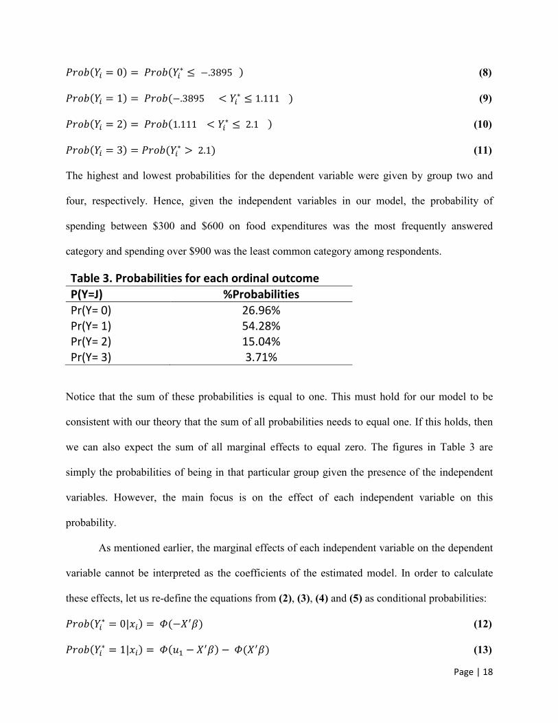
probabilities associated with each ordinal outcome can then be estimated with the help of these
parameters and can be denoted as follows:
�������� � �� � �������
� ���� (2)
�������� � � � ������� � ��
� � ��� (3)
�������� � �� � ������� � ��
� � ��� (4)
�������� � �� � �������
� � ��� (5)
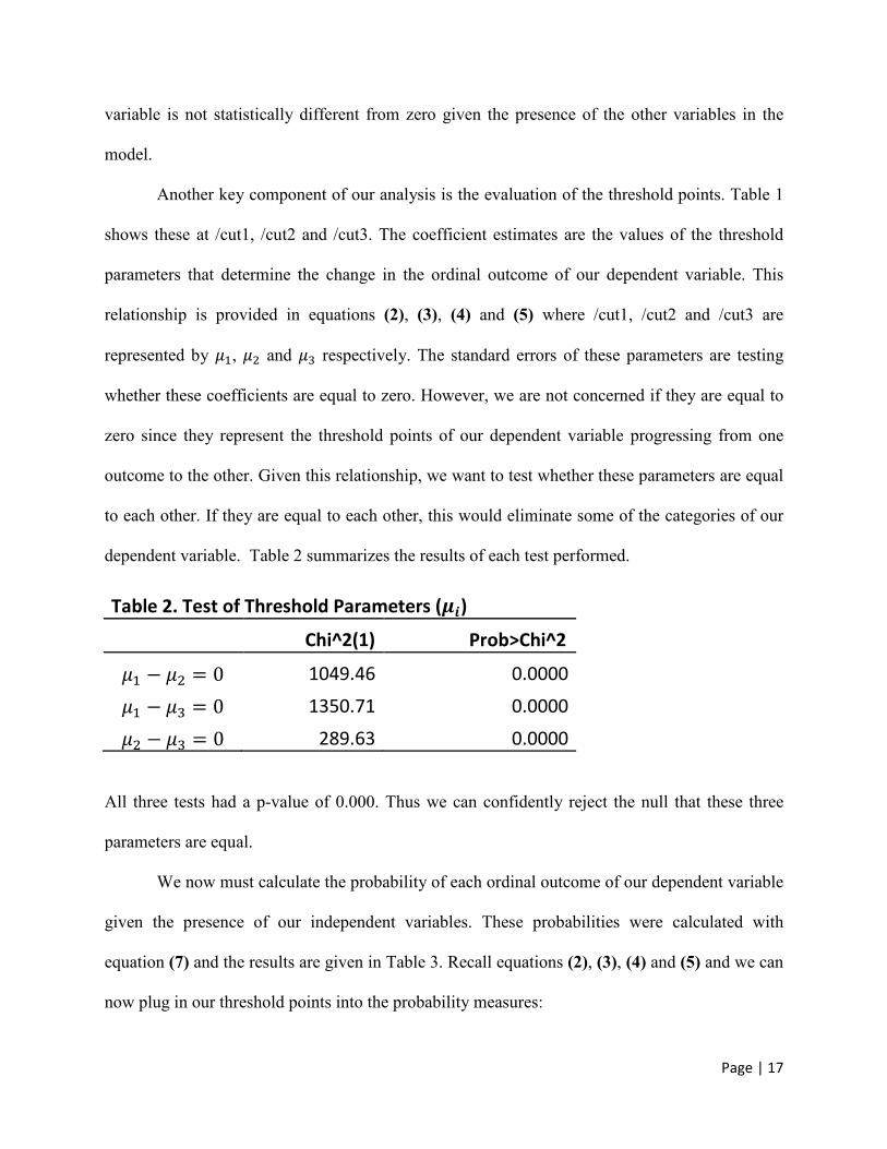
Each parameter ��represents a threshold for the probability of the dependent variable switching
from one category to the other.
The primary interest is to determine the affect of particular independent variables on the
dependent variable. Once a model has been estimated, coefficients are then computed to
determine these effects. If, for example, a linear regression model is estimated and coefficients
for each independent variable are computed, we can predict the change in the dependent variable
Page | 11
given a change in the independent variable ceteris paribus. These marginal effects are estimated
directly from these coefficients. For the ordered probit model, however, estimating these
marginal effects becomes a little more involved. The coefficients estimated in this type of model
do not represent the marginal effects and have no direct interpretation. This can be true for any
nonlinear regression analysis. To determine these effects, we can use the estimated coefficients
to calculate the probabilities of each ordinal outcome as well as their corresponding marginal
probabilities. The next section is intended to provide an explanation of each variable to be
included in the model and how it will be employed within the ordered probit model for this
study.
Dependent and Independent Variables
As mentioned above, the ordered probit model is used when the dependent variable can
have an outcome of more than two categories. Unlike the probit model which uses a binary
response, the ordered probit uses an ordinal response variable. The model to be estimated is as
All other marginal effects of our variable veggie are positive. The second largest affect is
in the third category of food expenditures. We can interpret this as being a vegetarian increases
the probability of spending between $600 and $900 by 2.70%. As demonstrated in table 4, all
marginal effects of the variable veggie are statistically significant. Thus, aside from the first food
expenditure category, begin a vegetarian increases the probability of spending over $300.
Specifically, as food expenditures increase, being a vegetarian will increase the probability of
being part of a higher ordinal category of monthly food expenditures.
Now let us consider the effect of organic food purchases. Recall that the variable organic
will take on a value of 1 if the consumer purchased organic foods in the past year and 0
Page | 22
otherwise. The largest affect is in the first ordinal category. A consumer that purchases organic
foods is 5.90% less likely of spending less than $300 on food expenditures than a consumer that
has not purchased organic foods. All marginal effects of organic are statistically significant.
Therefore, we can reject the null for all values and conclude that buying organic foods has a
significant effect on overall food expenditures. Specifically, as food expenditures increase, there
is a higher probability of being in a higher ranked ordinal category when a consumer has
purchased organic foods.
This particular trend is also the case for our dummy variable children. Similar to the
independent variables veggie and organic, there is a negative effect on the first ordinal category
of food expenditures and all other higher ranked ones are positive (refer to Table 4). The first
marginal effect for children is the largest effect in this study. However, this is expected due to
the nature of the dummy variable children. Recall that the marginal effect is the discrete change
of the dummy variable children from 0 to 1. If there were no children under the age of 18 present
in the respondent’s household, then children took on the value of 0 and 1 otherwise. Thus, the
probability of spending less than $300 on food expenditures decreased by 24.87% if there were
one or more children present in the household. Conversely, the probability of spending between
$600 and $900 increased by 15.29% when there were one or more children under the age of 18
present in the household. This dummy variable also had the largest Z value for all affects (except
for the marginal effect on the P(Y=1|children) where we failed to reject the null) which indicates
that it is the most statistically significant variable in our model.
The three variables discussed above all have a similar trend when it came to the
probability of our dependent variable, food expenditures. All three variables veggie, organic and
children negatively affected the lowest food expenditure category. The other three higher ranked
Page | 23
categories were positively affected by the presence of these variables. However, the three
remaining dummy variables (yage, sage and male) have the exact opposite effect on our
dependent variable.
Yage and sage are the two subcategories of the age specification of the respondent. Recall
that the middle aged category of 35 to 54 was dropped to avoid the dummy variable trap. The
dummy variable yage represents the younger aged group of 18 to 34. Evaluating Table 3, we can
see that there is a rather large effect on the probability of spending less than $300 on overall food
expenditure when the respondent was part of this age category. Specifically, the probability of
being in the first ordinal category of the dependent variable, food expenditures, increased by
19.87% if the respondent was aged 18 to 34. In contrast, the probability of being in a higher
ranked category of food expenditures decreased when the respondent was of this age category.
This result was expected given the type of respondent that would fall into this category.
Particularly, college and university students tend to spend less than a middle aged consumer that
might possess a family or significant other. It should also be noted that all values were
statistically significant for the dummy variable yage.
The dummy variable sage had a similar affect on the dependent variable. The probability
of spending less than $300 on food expenditures increased by 11.50% when the respondent was
aged 55 or over. Its affect on higher ranked ordinal categories was identical to the dummy
variable yage but slightly less pronounced and all values were also statistically significant.
The last dummy variable in our model identified the gender of the respondent. Similar to
the logic of dropping one of the age categories as mentioned above, the dummy variable for
females was dropped. The male coefficient estimate as well as all marginal effects of this
variable was not found to be statistically significant. Thus, we must conclude that the gender of a
Page | 24
consumer does not affect the probability of being in a particular ordinal outcome of food
expenditures. It should be noted that the relationship between gender and food expenditures
might not be prevalent in this study. However, further empirical work should consider the impact
of gender on vegetarian diets. Considering that our dependent variable was food expenditures,
this study was unable to identify the likelihood of being a vegetarian when one is male or female.
The study of this relationship might shed some light on the frequency of vegetarian diets as well
as the purchase behavior of this lifestyle.
Discussion and Final Remarks
As discussed previously, the literature on the economics of vegetarianism is very limited.
There have been no attempts, to this study’s knowledge, at evaluating the food expenditures a
consumer might face when following a vegetarian diet. Considering the amount of attention and
popularity this diet has accumulated, it is shocking that most of the claims being put forth are not
supported by empirical research. To fill this gap, this study attempted to address the claim that
vegetarians tend to have lower food expenditures than non-vegetarian consumers. We were able
to show that the probability of spending less than $300 on food expenditures decreased when a
consumer was a vegetarian. Conversely, the probability of being in a high ranked ordinal
category of food expenditures increased when a consumer followed a vegetarian diet.
In addition to evaluating the effects of a vegetarian diet, we also estimated the impact of
purchasing organic foods on food expenditures. Similar to the effect of a vegetarian diet on the
lowest ordinal outcome of food expenditures, purchasing organic foods also decreased the
probability of being in this category. Furthermore, every observation was statistically significant
in our model and thus we showed with confidence that purchasing organic foods increases
Page | 25
overall food expenditure. The next step to consider is the relationship between organic foods and
vegetarians. This study did not consider this relationship but does recommend further research on
this topic. Given that the market for organic foods will continue to increase, we need to
understand how particular food regimes affect purchasing behavior. If organic agriculture is part
of the “going green” initiative, then gathering information on “green” consumers and what type
of diet they are following is crucial for capturing the true potential of this market.
One thing to consider when analyzing these results is the fact that vegetarians are more
likely to be in the younger aged group. As mentioned earlier, generation Y consumers (born in
1980s and 1990s) demanded more cutting edge, exotic and vegetarian foods than any other
generation. We can also assume that a younger aged consumer will spend less on food
expenditures. They are more likely to be living a student life or have less income than a middle
aged consumer with a family and children to provide for. If this is the case, we would expect
vegetarians to fall within the lower food expenditure category. Taking this into consideration, it
should be noted that results found by this study are very sensitive to the current characteristics of
a vegetarian consumer. The relationship between a vegetarian and food expenditures might be
more pronounced if this study were to be evaluated in ten years from now. By that time,
generation Y will now be part of the middle aged category and possess more purchasing power
and disposable income. This might drastically alter the results found by this study.
Given all this information, we were still able to statistically prove that the probability of
spending less than $300 on food expenditures decreased when a consumer followed a vegetarian
diet and increased when food expenditures were higher than this amount. As mentioned earlier,
vegetarianism is a growing trend among today’s green society. We cannot ignore its growth nor
can we assume that its followers have little impact on the overall food market. Canada’s market
Page | 26
for vegetarian foods might be minimal, but we must also consider the type of consumer currently
living and immigrating to this country. Between the years 1990 to 2000, 40% of Canada’s
immigration came from several Asian countries such as China, Pakistan, Taiwan and India
(Oliveira, 2003). Although some of these countries do not follow a pure vegetarian lifestyle, they
tend to consume more plant-based foods.
Although still a young market, vegetarianism is proving itself as an emerging force
within today’s food demand market. It is also very versatile in terms of its overall marketability.
Specifically, it is not restricted to pure vegetarians or vegans. Non-vegetarians seeking a
healthier or meat-less option once or twice a week can also purchase these types of foods. Also,
the number of vegetarian restaurants continues to grow, and vegetarian options are being added
to everyday restaurant menus in order to accommodate for this new demand. A new market is
emerging and in order to fully capture its potential, new research is needed to empirically
understand its benefits as well as its costs.
Page | 27
References
1. Agriculture and Agri-Food Canada. “Consumption Trends to 2020.” Available from http: //www4.agr.gc.ca/AAFC-AAC/display-afficher.do?id=1201554109150&lang=eng. Accessed September 21st, 2010.
2. Alley, Holly. “Vegetarianism” University of Georgia, Cooperative Extension Service, Athens, GA. Available from http://www.fcs.uga.edu/pubs/current/FDNS-E-18.html; Accessed November 13th, 2010.
3. Blay-Palmer, Alison. “Growing Innovation Policy: The Case of Organic Agriculture in Ontario, Canada.” Environment and Planning C: Government and Policy, Vol 23, No. 4. (2005), pp. 557-581.
4. Canadian Wheat Board, Newsroom “A Few Facts.” Available from http://www.cwb.ca/ public/en/newsroom/releases/2009/091709.jsp; Accessed September 20th, 2010.
5. Dimitri, Carolyn., and Catherine Greene. “Recent Growth Patterns in the U.S. Organic Foods Market” Agriculture Information Bulletin No. (AIB777) (2002), pp.42(1-27).
6. Guido, Gianluigi. “The role of ethics and product personality in the intention to purchase organic food products: a structural equation modeling approach,” International Review of Economics, Vol. 57, No. 1. (2010), pp. 79-102.
7. Honkanen, Pirjo., and Bar Verplanken. “Ethical Values and Motives Driving Organic Food Choice” Journal of Consumer Behavior, Vol. 5, No.5 (2006), pp.420-430.
8. Lusk, Jayson L. “Some Economic Benefits and Costs of Vegetarianism” Agricultural and Applied Economics Association, Vol 38, No. 2. (October 2009), pp. 109-124.
9. Olivera, Sarah. “Vegetarianism – A Meatless Eating Experience” Alberta Agriculture, Food and Rural Development. Government of Alberta, August, 2003. Available from http://www1.agric.gov.ab.ca/$department/deptdocs.nsf/all/sis8739/$file/vegetarianism.pdf?OpenElement; Accessed November 13th, 2010.
10. Onyango, Benjamin., and William Hallman. “Purchasing Organic Food in U.S. Food Systems: A Study of Attitudes and Practice.” Agricultural and Applied Economics Association, Meeting (July 23-26, 2006)