Food Store Location AnalysisAlbuquerque New Mexico, 2010

Prepared for: Geography 586L - Spring Semester, 2014

Larry Spear M.A., GISPSr. Research Scientist (Ret.)

Division of Government ResearchUniversity of New Mexico

http://www.unm.edu/~lspear

Preliminary (OLS-Global) Version – Update 4/19/14

Preface

• Follow-up to thesis research completed, 1982• Also Applied Geography Conference, 1985• Previous work using 1970 and 1980 data• Used state-of-art technology at the time• Pen and Ink and Zip-a-Tone (decal) cartography• SAS (Statistical Analysis System)• ESRI’s Automap II (first product) and Fortran• IBM Mainframe computer at UNM• Updates with recent GIS and statistical facilities –

OLS (Global) and GWR (Local) versions planned

Research Project Components

• A well defined research project should address- Theory (previous research and practice)- Method (established and proposed

statistical and spatial techniques)- Application/Results (maps, tables,

charts, and future research)• This presentation follows this outline

Theory

• Economic Geography and Retail Geography (sub field)-Food stores are lower-order retail service-Tend to locate close to residential customer

population they are intended to serve• Most previous research focused on customer shopping

patterns-Delineation of trade or market areas-Based on rational customers (consumers) who shop

at closest store???• Also proprietary sales (geocoded customer location) data

collected by individual companies (*Not Shared)

Method

• Can a method be employed (developed) to:-Test assumption (hypothesis) that full-service food

stores tend to locate with respect to residential population• Needs to use readily available (non-proprietary) store and

population (potential customer) data• Should be easy to apply with generally available GIS and

statistical software• Should be useful to others (not just supermarket

corporations) like city planners and small business owners

Method – Gravity Model

• Gravity model developed to measure overall opportunity (retail coverage) available to customers provided by location and size of all stores

• Potential shopping choices without any assumption of customers just shopping at the closest store

• Spatial Interaction – closer larger stores are more attractive than smaller distant stores.

Spatial Interaction and Distance Decay

Method – Ordinary Least Squares Regression (OLS - Global)

• Measure of retail coverage (gravity model) statistically compared with population

• Population from 2010 Census block groups (count and population density)

• Regression determines the expected (predicted or “average”) retail coverage value(s) given observed population (count and density) values:

• determine relatively over (+), under (-), or adequate (≈0) serviced areas (map of standard residuals, observed - expected)

Positive (+)

Negative (-)

Residual = Observed Y – Predicted YESRI Graphic ?

Residual = Observed - Predicted

Application – (Analysis Results)

• ArcGIS ModelBuilder used to perform analysis and produce the maps (layers) – IDW and OLS Tools – also SPSS, Minitab, and R for statistics

• Layer 1 – Food Store Density, approximate size of store (n=59, ArcGIS World Imagery, Geocoding)

• Layer 2 – Population Density per square kilometer by census block group 2010 (n=417)

• Layer 3 – Retail Coverage from Gravity Model• Layer 4 – Retail Servicing from regression (OLS –

Global), map of standardized residuals

ArcGIS ModelBuilder and Regression (OLS) Results (Preliminary March, 2014)

Linear Regression Assumptions and Diagnostics*Geographic data never meets all assumptions

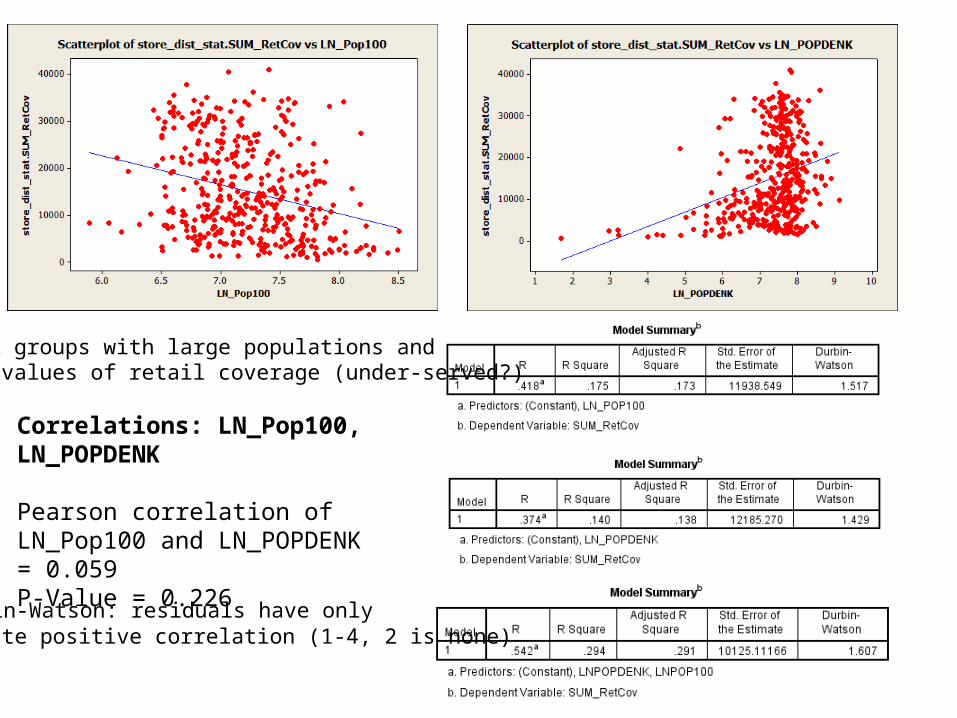
• Normally distributed (kinda OK) – transformations of population (LnPOP100), and population density (POPDENK to LnPOPDENK?)

• Multicollinearity (OK?) – LnPOP100 and LnPOPDENK not globally but locally correlated

• Redundant variables (OK) – VIF much less than 7.5• Linear relationship (Violation) – LnPOP100 curvilinear (biased?)• Normally distributed standard residuals (OK?), Jarque-Bera*

significant, also non-linear relationship• Residual heteroscedasticity (Violation) – residuals increase with

value of independent variables (non-constant variance)• Nonstationary spatial relationships – Robust_Pr (OK), Koenker p* • Possible solution – Geographically Weighted Regression (GWR -

Local) may improve results, OLS OK for initial study (“models the average relationship” not used as a predictive model), <AICc better

Sum_RetCov = 76284.3 -10844.3(LnPOP100) + 5365.0(LnPOPDENK)*Preliminary Results (March, 2014)

ArcGIS ModelBuilder and Regression(OLS-Global) Results (Preliminary March, 2014)

Correlations: LN_Pop100, LN_POPDENK

Pearson correlation of LN_Pop100 and LN_POPDENK = 0.059P-Value = 0.226

*Durbin-Watson: residuals have only moderate positive correlation (1-4, 2 is none)

*Block groups with large populations andsmall values of retail coverage (under-served?)

Standard Residuals

OLS Regression

Preliminary ResultsMarch, 2014

Note: Residual clustering isexpected for this application

Base Data Layers

Legend

Food Stores

Major Roads

High : 11111.7

Low : 0.0259983

Food Store Density

±0 5 10 15 202.5

Miles

Population Density

Legend

ABQ Major Roads

High : 8794.37

Low : 0.00808593

Analysis (Results) LayersPreliminary Results (March, 2014)

Retail Coverage Retail Servicing

Legend

Food Stores

Major Roads

High : 62733.6

Low : 0.438917

Legend

Food Stores

Major Roads

-2.401698112 - -1.5

-1.499999999 - -0.5

-0.5 - 0.5

0.5 - 1.5

1.500000001 - 2.5

0 5 10 15 202.5Miles

±

OLS (R2a=.291) and GWR(R2a=.716)

VARNAME VARIABLE

Bandw idth 5650.152102

ResidualSquares 16174172106.31266

EffectiveNumber 22.41857

Sigma 6402.398599

AICc 8505.980062

R2 0.730943

R2Adjusted 0.716338

What Next?

• Further validation of store food areas (determine and exclude non-food areas) by field survey

• Use Manhattan and Network distances• Apply Geographically Weighted Regression (GWR) –

Need to learn (study) more about this local technique!• Updates for 2014 stores (gain and loss) and updated

population estimates• ArcGIS Server (on ArcGIS Online)• Develop Python script (on ArcGIS Resources)• Presentation(s) and Publication