Page 1
8/4/2019 Forecasting 2008
http://slidepdf.com/reader/full/forecasting-2008 1/67
Demand Forecasting
• Four Fundamental Approaches• Time Series „„„
– General Concepts – Evaluating Forecasts – How ‗good‘ is it? – Forecasting Methods (Stationary) Š
• Cumulative Mean Š• Naïve Forecast ŠŠ„ŠŠŠŠ• Moving Average• Exponential Smoothing
– Forecasting Methods (Trends & Seasonality)• OLS Regression• Holt‘s Method• Exponential Method for Seasonal Data• Winter‘s Model Other Models
Page 2
8/4/2019 Forecasting 2008
http://slidepdf.com/reader/full/forecasting-2008 2/67
Demand Forecasting
• Forecasting is difficult – especially for the future• Forecasts are always wrong• The less aggregated, the lower the accuracy• The longer the time horizon, the lower the accuracy
• The past is usually a pretty good place to start• Everything exhibits seasonality of some sort• A good forecast is not just a number – it should include a
range, description of distribution, etc.• Any analytical method should be supplemented by
external information• A forecast for one function in a company might not beuseful to another function (Sales to Mkt to Mfg to Trans)
Page 3
8/4/2019 Forecasting 2008
http://slidepdf.com/reader/full/forecasting-2008 3/67
Four Fundamental Approaches
Subjective – Judgmental
• Sales force surveys• Delphi techniques• Jury of experts
– Experimental
• Customer surveys• Focus group sessions• Test Marketing
Objective – Causal / Relational
• Econometric Models• Leading Indicators• Input-Output Models
– Time Series
• ―Black Box‖ Approach • Uses past to predict
the future
Page 4
8/4/2019 Forecasting 2008
http://slidepdf.com/reader/full/forecasting-2008 4/67
Time Series Concepts
1. Time Series – Regular & recurring basis to forecast2. Stationarity – Values hover around a mean3. Trend- Persistent movement in one direction4. Seasonality – Movement periodic to calendar
5. Cycle – Periodic movement not tied to calendar6. Pattern + Noise – Predictable and random components of aTime Series forecast
7. Generating Process –Equation that creates TS8. Accuracy and Bias – Closeness to actual vs Persistent
tendency to over or under predict9. Fit versus Forecast – Tradeoff between accuracy to past
forecast to usefulness of predictability10. Forecast Optimality – Error is equal to the random noise
Page 5
8/4/2019 Forecasting 2008
http://slidepdf.com/reader/full/forecasting-2008 5/67
Page 6
8/4/2019 Forecasting 2008
http://slidepdf.com/reader/full/forecasting-2008 6/67
Demand Forecasting
• Generate the large number of short-term, SKUlevel, locally dis-aggregated demand forecastsrequired for production, logistics, and sales to
operate successfully. „• Focus on: ŠŠŠŠŠ – Forecasting product demand – Mature products (not new product releases)
– Short time horizon (weeks, months, quarters, year) – Use of models to assist in the forecast – Cases where demand of items is independent
Page 7
8/4/2019 Forecasting 2008
http://slidepdf.com/reader/full/forecasting-2008 7/67
Historical Data
0 50
100 150 200 250 300 350 400
0 10 20 30 40 50
Forecasting Terminology
Initialization ExPostForecast
Forecast
Historical Data
Page 8
8/4/2019 Forecasting 2008
http://slidepdf.com/reader/full/forecasting-2008 8/67
―We are now looking at a future from here, and thefuture we were looking at in February now includessome of our past, and we can incorporate the past
into our forecast. 1993, the first half, which is nowthe past and was the future when we issued our firstforecast, is now over‖
Laura D‘Andrea Tyson, Head of the President‘s Council of Economic Advisors, quoted in November of 1993 in the Chicago Tribune , explaining why the Administration reduced its projectionsof economic growth to 2 percent from the 3.1percent it predicted inFebruary.
Forecasting Terminology
Page 9
8/4/2019 Forecasting 2008
http://slidepdf.com/reader/full/forecasting-2008 9/67
Forecasting Problem
• Suppose your fraternity/sorority houseconsumed the following number of cases ofbeer for the last 6 weekends: 8, 5, 7, 3, 6, 9
0
1
23
4
5
6
7
8
9
10
0 1 2 3 4 5 6 7
Week
C a s e s
• How many casesdo you think yourfraternity / sorority
will consume thisweekend?
Page 10
8/4/2019 Forecasting 2008
http://slidepdf.com/reader/full/forecasting-2008 10/67
0 1 2 3 4 5 6 7 8 9 10
0 1 2 3 4 5 6 7 8 Week
C a s e s
Forecasting:Simple Moving Average Method
• Using a three period moving average, wewould get the following forecast:
63
963F
Page 11
8/4/2019 Forecasting 2008
http://slidepdf.com/reader/full/forecasting-2008 11/67
0 1 2 3 4 5 6 7 8 9 10
0 1 2 3 4 5 6 7 8 Week
C a s e s
Forecasting:Simple Moving Average Method
• What if we used a two period moving average?
5.72
96F
Page 12
8/4/2019 Forecasting 2008
http://slidepdf.com/reader/full/forecasting-2008 12/67
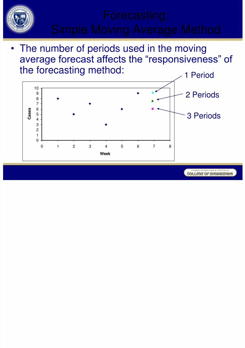
• The number of periods used in the movingaverage forecast affects the ―responsiveness‖ of the forecasting method:
0 1 2 3 4 5 6 7 8 9 10
0 1 2 3 4 5 6 7 8 Week
C a s e s
Forecasting:Simple Moving Average Method
2 Periods
3 Periods
1 Period
Page 13
8/4/2019 Forecasting 2008
http://slidepdf.com/reader/full/forecasting-2008 13/67
t A(t) F(t)1 8
2 5
3 7
4 3 6.67
5 6 5
6 9 5.33
7 68 6
9 6
10 6
Forecasting Terminology
• Applying this terminology to our problemusing the Moving Average forecast:
Initialization
ExPostForecast
Forecast
ModelEvaluation
Page 14
8/4/2019 Forecasting 2008
http://slidepdf.com/reader/full/forecasting-2008 14/67
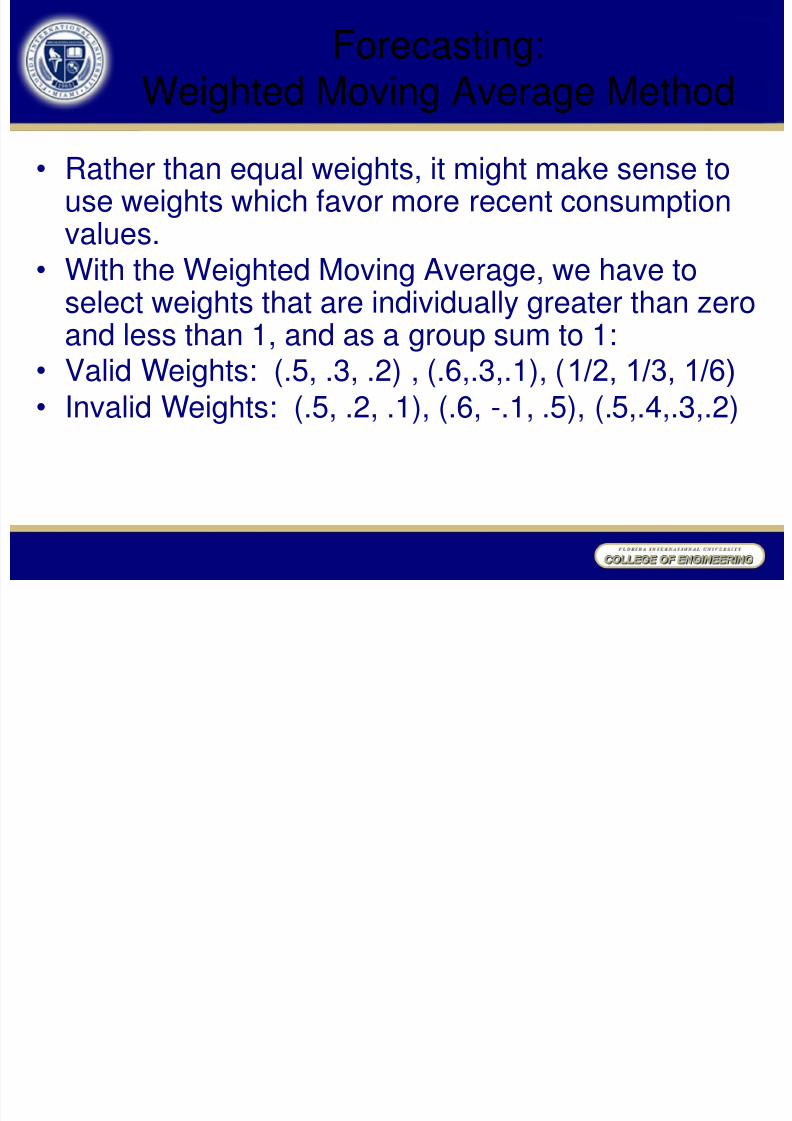
• Rather than equal weights, it might make sense touse weights which favor more recent consumptionvalues.
• With the Weighted Moving Average, we have toselect weights that are individually greater than zeroand less than 1, and as a group sum to 1:
• Valid Weights: (.5, .3, .2) , (.6,.3,.1), (1/2, 1/3, 1/6)
• Invalid Weights: (.5, .2, .1), (.6, -.1, .5), (.5,.4,.3,.2)
Forecasting:Weighted Moving Average Method
Page 15
8/4/2019 Forecasting 2008
http://slidepdf.com/reader/full/forecasting-2008 15/67
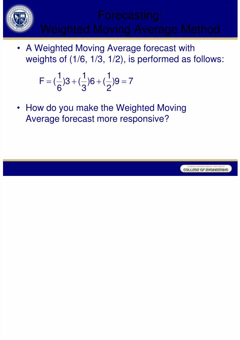
Forecasting:Weighted Moving Average Method
• A Weighted Moving Average forecast withweights of (1/6, 1/3, 1/2), is performed as follows:
• How do you make the Weighted MovingAverage forecast more responsive?
79)2
1
(6)3
1
(3)6
1
(F
Page 16
8/4/2019 Forecasting 2008
http://slidepdf.com/reader/full/forecasting-2008 16/67
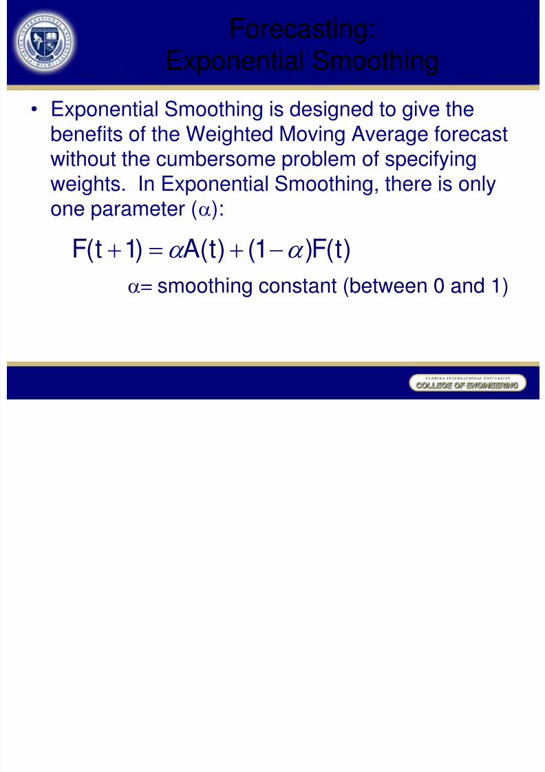
• Exponential Smoothing is designed to give thebenefits of the Weighted Moving Average forecastwithout the cumbersome problem of specifying
weights. In Exponential Smoothing, there is onlyone parameter ():
= smoothing constant (between 0 and 1)
Forecasting:Exponential Smoothing
)t(F)1()t(A)1t(F
Page 17
8/4/2019 Forecasting 2008
http://slidepdf.com/reader/full/forecasting-2008 17/67
Initialization:•
• )2(F)1()2(A)3(F
)1(A)2(F
Forecasting:Exponential Smoothing
)2(F)1()2(A)3(F
2 / )]2(A)1(A[)2(F
Page 18
8/4/2019 Forecasting 2008
http://slidepdf.com/reader/full/forecasting-2008 18/67
t A(t) F(t)
1 8
2 5 6.5
3 7 5.9
4 3 6.34
5 6 5
6 9 5.4
7 6.84
8 6.84
9 6.84
10 6.84
Forecasting:Exponential Smoothing
• Using = 0.4,
Initialization
ExPostForecast
Forecast
Page 19
8/4/2019 Forecasting 2008
http://slidepdf.com/reader/full/forecasting-2008 19/67
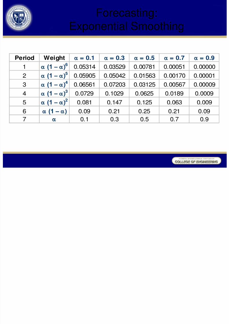
Forecasting:Exponential Smoothing
Period Weight 0.1 0.3 0.5 0.7 0.9
1 (1 – )6
0.05314 0.03529 0.00781 0.00051 0.00000
2 (1 – )5
0.05905 0.05042 0.01563 0.00170 0.00001
3 (1 – )4 0.06561 0.07203 0.03125 0.00567 0.00009
4 (1 – )3 0.0729 0.1029 0.0625 0.0189 0.0009
5 (1 – )2
0.081 0.147 0.125 0.063 0.009
6 (1 – ) 0.09 0.21 0.25 0.21 0.09
7 0.1 0.3 0.5 0.7 0.9
Page 20
8/4/2019 Forecasting 2008
http://slidepdf.com/reader/full/forecasting-2008 20/67
Forecasting:Exponential Smoothing
0 0.1 0.2 0.3 0.4 0.5 0.6 0.7 0.8 0.9
1
1 2 3 4 5 6 7 Period
W e i g h t
= 0.1 = 0.3 = 0.5 = 0.7 = 0.9
Page 21
8/4/2019 Forecasting 2008
http://slidepdf.com/reader/full/forecasting-2008 21/67
Outliers (eloping point)
Exp Exp
t A(t) = 0.3 = 0.7
1 8
2 5 6.50 6.50
3 6 6.05 5.454 3 6.04 5.84
5 4 5.12 3.85
6 15 4.79 3.96
7 7.85 11.69
8 7.85 11.699 7.85 11.69
10 7.85 11.69
0
2
4
6
8
10
12
14
16
1 2 3 4 5 6 7 8 9 10
Outlier
Page 22
8/4/2019 Forecasting 2008
http://slidepdf.com/reader/full/forecasting-2008 22/67
Data with Trends
01
2
3
4
5
67
8
9
10
0 1 2 3 4 5 6 7
Page 23
8/4/2019 Forecasting 2008
http://slidepdf.com/reader/full/forecasting-2008 23/67
0 1 2
3 4 5 6 7 8 9
10
1 2 3 4 5 6 7
A(t)
Data with Trends
= 0.3 = 0.5 = 0.7 = 0.9
Page 24
8/4/2019 Forecasting 2008
http://slidepdf.com/reader/full/forecasting-2008 24/67
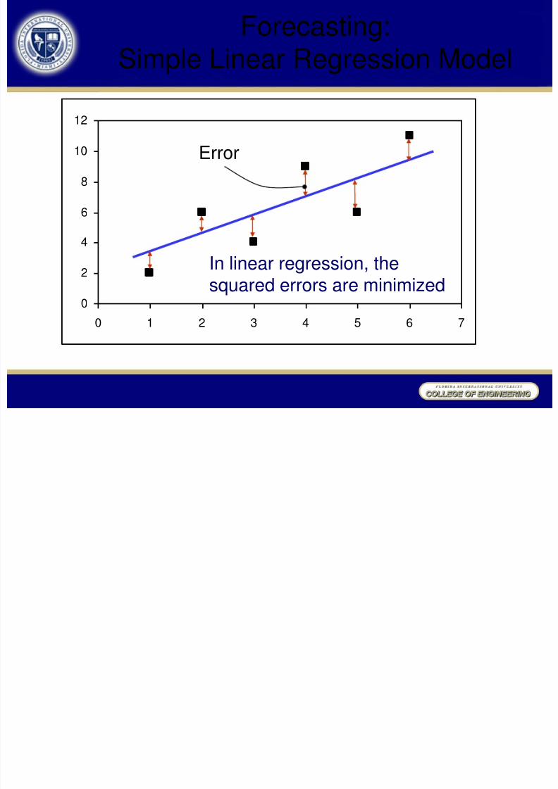
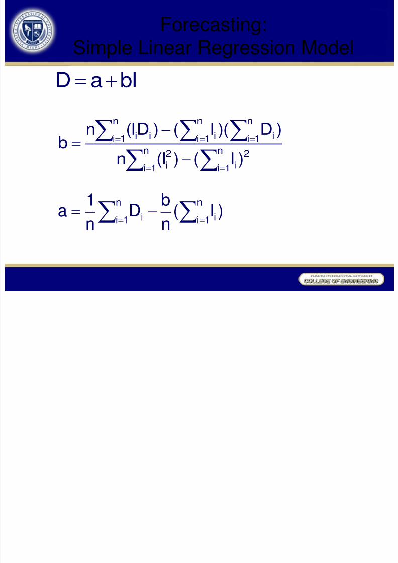
Forecasting:Simple Linear Regression Model
Simple linear regressioncan be used to forecastdata with trends
D is the regressed forecast value or dependentvariable in the model, a is the intercept value of theregression line, and b is the slope of the regressionline.
a
bIaD
D
0 1 2 3 4 5 I
b
Page 25
8/4/2019 Forecasting 2008
http://slidepdf.com/reader/full/forecasting-2008 25/67
0
2
4
6
8
10
12
0 1 2 3 4 5 6 7
Forecasting:Simple Linear Regression Model
In linear regression, the
squared errors are minimized
Error
Page 26
8/4/2019 Forecasting 2008
http://slidepdf.com/reader/full/forecasting-2008 26/67
Forecasting:Simple Linear Regression Model
n
1i
n
1i
2
i
2
i
n
1i
n
1i
n
1i iiii
)I()I(n
)D)(I()DI(nb
bIaD
n
1in
1i ii )I(nbD
n1a
Page 27
8/4/2019 Forecasting 2008
http://slidepdf.com/reader/full/forecasting-2008 27/67
0 50
100 150 200 250
0 2 4 6 8 10 12 14 16
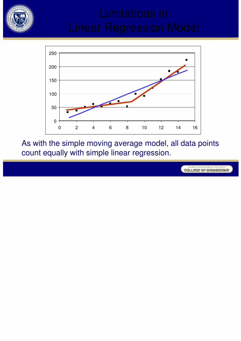
Limitations inLinear Regression Model
As with the simple moving average model, all data pointscount equally with simple linear regression.
Page 28
8/4/2019 Forecasting 2008
http://slidepdf.com/reader/full/forecasting-2008 28/67
Forecasting:Holt‘s Trend Model
• To forecast data with trends, we can usean exponential smoothing model withtrend, frequently known as Holt‘s model:
L(t) = A(t) + (1- ) F(t) T(t) = [L(t) - L(t-1) ] + (1- ) T(t-1)
F(t+1) = L(t) + T(t)• We could use linear regression to initialize
the model
Page 29
8/4/2019 Forecasting 2008
http://slidepdf.com/reader/full/forecasting-2008 29/67
Holt‘s Trend Model: Initialization
t A(t)
1 32
2 38
3 50
4 61
5 526 63
7 72
8 53
9 99
10 92
11 12112 153
13 183
14 179
15 224
First, we‘ll initialize the model: x y x2 xy
1 32 1 32
2 38 4 76
3 50 9 150
4 61 16 244Sum 30 502
Average 2.5 45.25
5.20)(9.9)(2.5-45.3=xb-y=a
9.95
5.49
)5.2(430
.5)4(45.25)(2-502=
)xn(-x
)x)(yn(-xy=b
222
L(4) = 20.5+4(9.9)=60.1T(4) = 9.9
Page 30
8/4/2019 Forecasting 2008
http://slidepdf.com/reader/full/forecasting-2008 30/67
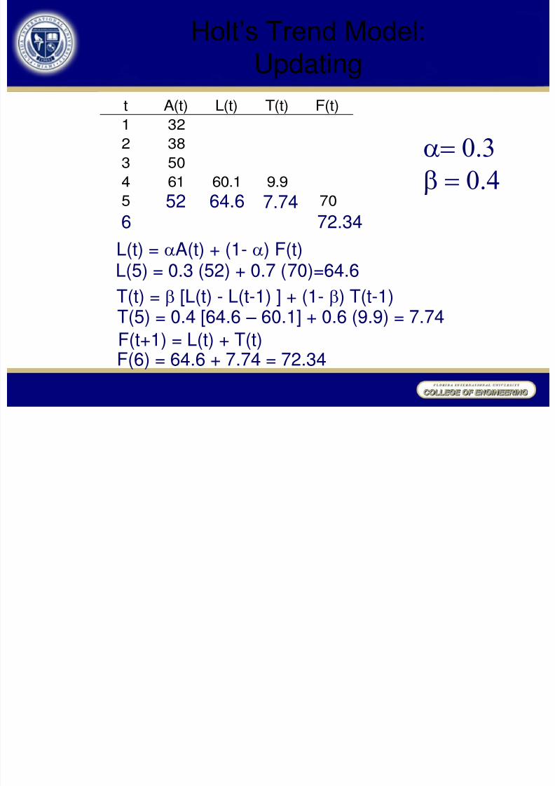
Holt‘s Trend Model: Updating
t A(t) L(t) T(t) F(t)
1 32
2 38
3 50
4 61 60.1 9.9
5 7052
L(t) = A(t) + (1- ) F(t)
0.3
0.4
L(5) = 0.3 (52) + 0.7 (70)=64.6
T(t) = [L(t) - L(t-1) ] + (1- ) T(t-1)T(5) = 0.4 [64.6 – 60.1] + 0.6 (9.9) = 7.74F(t+1) = L(t) + T(t)F(6) = 64.6 + 7.74 = 72.34
64.6 7.7472.346
Page 31
8/4/2019 Forecasting 2008
http://slidepdf.com/reader/full/forecasting-2008 31/67
t A(t) L(t) T(t) F(t)
1 32
2 38
3 50
4 61 60.1 9.9
5 52 64.60 7.74 70
6 72.34
Holt‘s Trend Model: Updating
63
0.3
0.4
L(6) = 0.3 (63) + 0.7 (72.34)=69.54T(6) = 0.4 [69.54 – 64.60] + 0.6 (7.74) = 6.62
F(7) = 69.54 + 6.62 = 76.16
69.54 6.6276.167 72
Page 32
8/4/2019 Forecasting 2008
http://slidepdf.com/reader/full/forecasting-2008 32/67
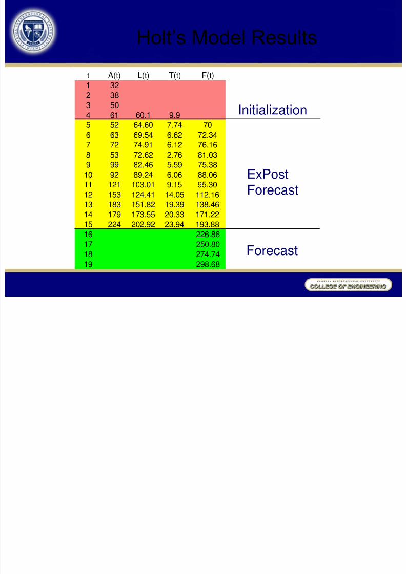
Holt‘s Model Results
t A(t) L(t) T(t) F(t)
1 32
2 38
3 50
4 61 60.1 9.9
5 52 64.60 7.74 70
6 63 69.54 6.62 72.34
7 72 74.91 6.12 76.16
8 53 72.62 2.76 81.03
9 99 82.46 5.59 75.38
10 92 89.24 6.06 88.06
11 121 103.01 9.15 95.30
12 153 124.41 14.05 112.16
13 183 151.82 19.39 138.46
14 179 173.55 20.33 171.22
15 224 202.92 23.94 193.88
16 226.86
17 250.80
18 274.74
19 298.68
Initialization
ExPostForecast
Forecast
Page 33
8/4/2019 Forecasting 2008
http://slidepdf.com/reader/full/forecasting-2008 33/67
Regression
0 50
100 150 200 250 300 350
0 5 10 15 20
Initialization ExPost Forecast Forecast
Holt‘s Model Results
Page 34
8/4/2019 Forecasting 2008
http://slidepdf.com/reader/full/forecasting-2008 34/67
Forecasting: Seasonal Model (No Trend)
0
5
10
15
20
25
30
35
40
45
50
S p r i n g 2
0 0 3
S u m m
e r 2 0
0 3
F a l l 2
0 0 3
W i n t
e r 2 0 0 3
S p r i n g 2
0 0 4
S u m m
e r 2 0
0 4
F a l l 2
0 0 4
W i n t
e r 2 0 0 4
S p r i n g 2
0 0 5
S u m m
e r 2 0
0 5
F a l l 2
0 0 5
W i n t
e r 2 0 0 5
A(t)
2003 Spring 16
Summer 27
Fall 39Winter 22
2004 Spring 16
Summer 26
Fall 43
Winter 23
2005 Spring 14Summer 29
Fall 41
Winter 22
Page 35
8/4/2019 Forecasting 2008
http://slidepdf.com/reader/full/forecasting-2008 35/67
L(t) = A(t) / S(t-p) + (1- ) L(t-1)
S(t) = g [A(t) / L(t)] + (1- g) S(t-p)
Seasonal Model Formulas
p is the number of periods in a season
Quarterly data: p = 4Monthly data: p = 12
F(t+1) = L(t) * S(t+1-p)
Page 36
8/4/2019 Forecasting 2008
http://slidepdf.com/reader/full/forecasting-2008 36/67
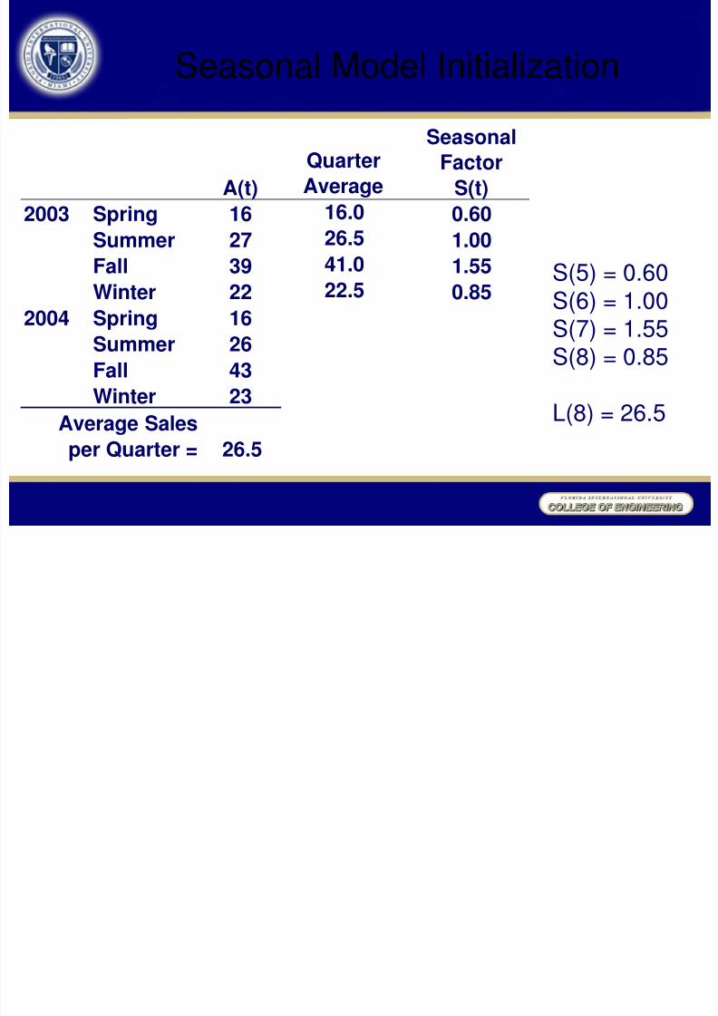
Seasonal Model Initialization
S(5) = 0.60S(6) = 1.00S(7) = 1.55S(8) = 0.85
L(8) = 26.5
Quarter Average
16.0 26.5 41.0 22.5
Seasonal Factor
S(t) 0.60 1.00
1.55 0.85
Average Sales per Quarter = 26.5
A(t) 2003 Spring 16
Summer
27
Fall 39 Winter 22
2004 Spring 16 Summer 26 Fall 43 Winter 23
Page 37
8/4/2019 Forecasting 2008
http://slidepdf.com/reader/full/forecasting-2008 37/67
Seasonal Model Forecasting
g 0.3
0.4
26.71 1.03 25.18 26.62 1.55 41.32 25.18 0.59 16.00 2005 Spring 14
Summer 29 Fall 41 Winter 22 26.34 0.84 22.60 2006 Spring Summer Fall Winter
15.53 27.02 40.69 22.25
A(t) L(t) Seasonal
Factor S(t) F(t)
2004 Spring 16 0.60 Summer 26 1.00 Fall 43 1.55 Winter 23 26.50 0.85
Page 38
8/4/2019 Forecasting 2008
http://slidepdf.com/reader/full/forecasting-2008 38/67
0 5
10 15 20 25 30 35 40 45 50
0 2 4 6 8 10 12 14 16
Seasonal Model Forecasting
Page 39
8/4/2019 Forecasting 2008
http://slidepdf.com/reader/full/forecasting-2008 39/67
Forecasting: Winter‘s Model for Data
with Trend and Seasonal Components
L(t) = A(t) / S(t-p) + (1- )[L(t-1)+T(t-1)]
T(t) = [L(t) - L(t-1)] + (1- ) T(t-1)
S(t) = g [A(t) / L(t)] + (1- g) S(t-p)
F(t+1) = [L(t) + T(t)] S(t+1-p)
Page 40
8/4/2019 Forecasting 2008
http://slidepdf.com/reader/full/forecasting-2008 40/67
Seasonal-Trend ModelDecomposition
• To initialize Winter‘s Model, we will use
Decomposition Forecasting, which itselfcan be used to make forecasts.
Page 41
8/4/2019 Forecasting 2008
http://slidepdf.com/reader/full/forecasting-2008 41/67
41
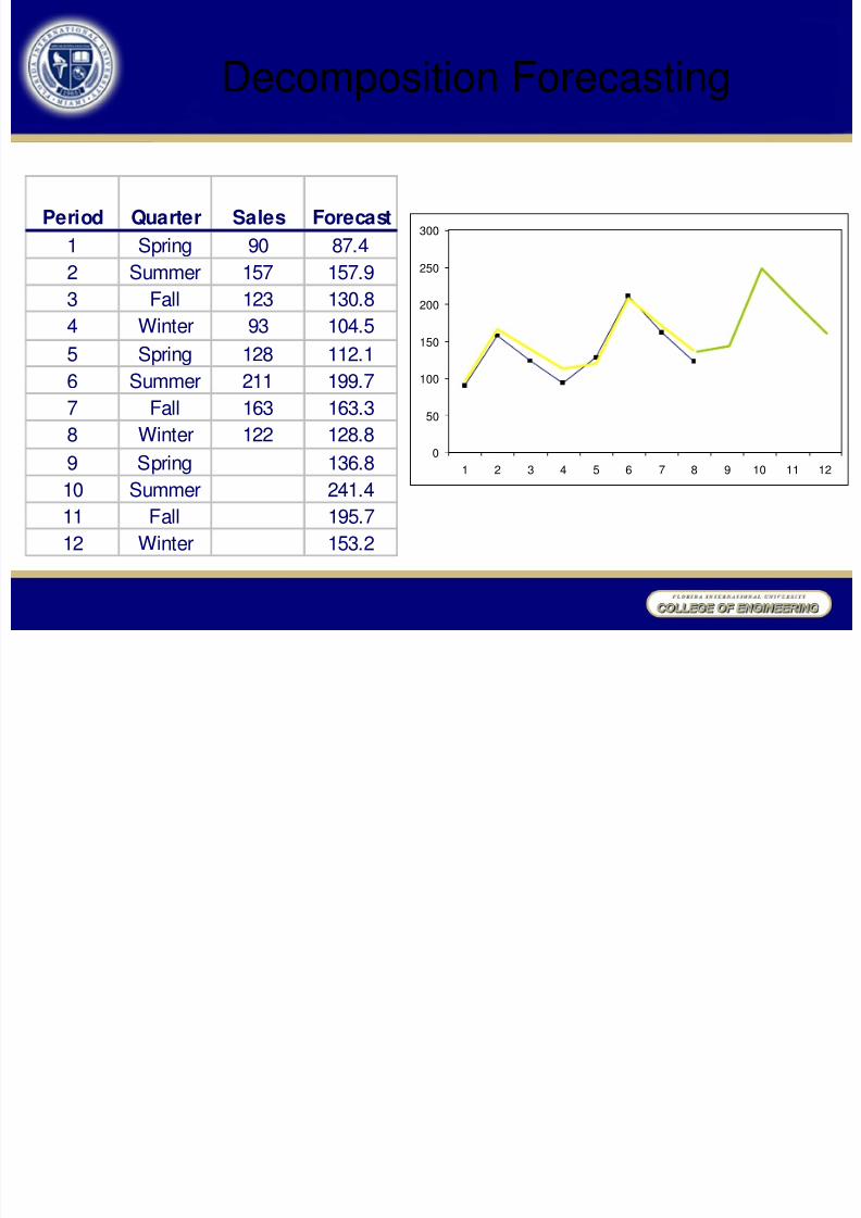
Decomposition Forecasting
• There are two ways to decompose forecastdata with trend and seasonal components:
– Use regression to get the trend, use the trendline to get seasonal factors
– Use averaging to get seasonal factors, ―de-seasonalize‖ the data, then use regression to
get the trend.
Page 42
8/4/2019 Forecasting 2008
http://slidepdf.com/reader/full/forecasting-2008 42/67
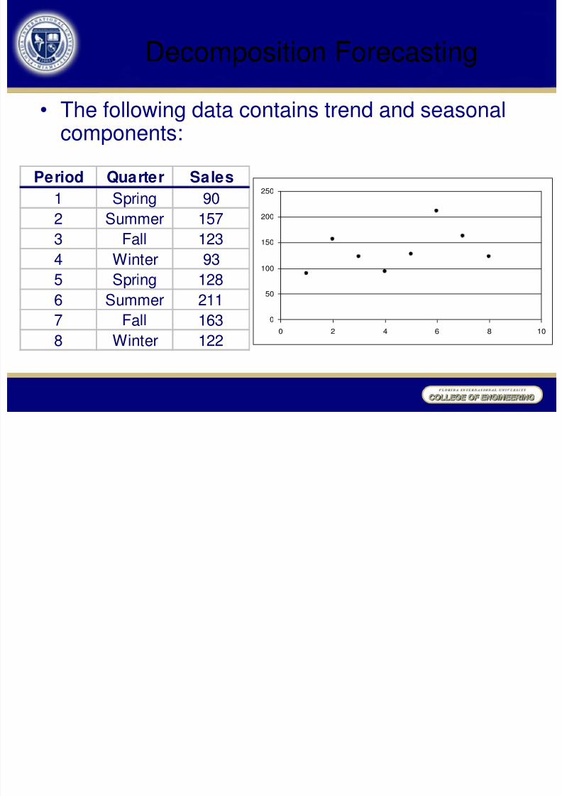
Decomposition Forecasting
• The following data contains trend and seasonalcomponents:
0
50
100
150
200
250
0 2 4 6 8 10
Period Quarter Sales
1 Spring 902 Summer 157
3 Fall 123
4 Winter 93
5 Spring 128
6 Summer 211
7 Fall 163
8 Winter 122
Page 43
8/4/2019 Forecasting 2008
http://slidepdf.com/reader/full/forecasting-2008 43/67
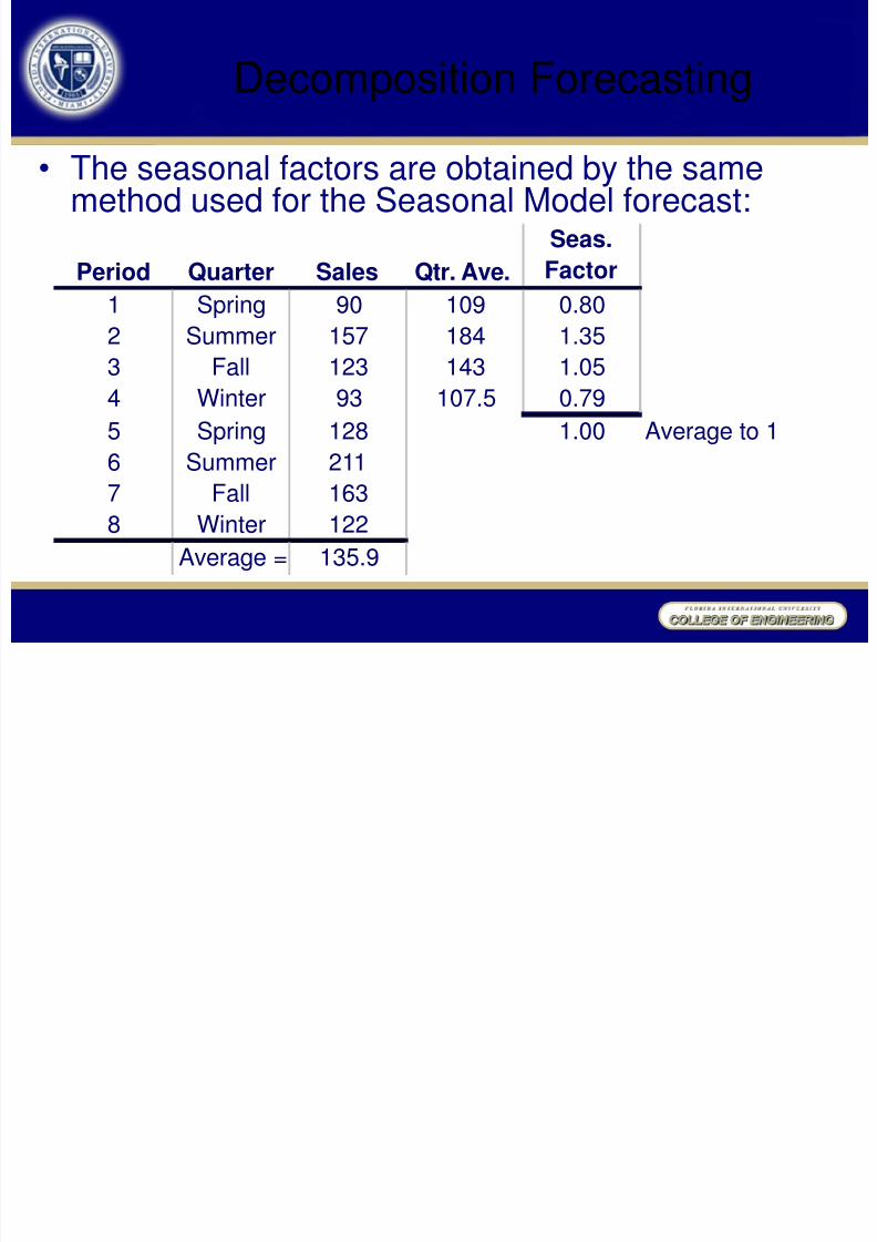
Decomposition Forecasting
• The seasonal factors are obtained by the samemethod used for the Seasonal Model forecast:
Period Quarter Sales 1 Spring 90 2 Summer 157 3 Fall 123 4 Winter 93 5 Spring 128 6 Summer 211 7 Fall 163 8 Winter 122
Average = 135.9
Average to 1
Qtr. Ave. 109 184 143
107.5
Seas.
Factor 0.80 1.35 1.05 0.79 1.00
Page 44
8/4/2019 Forecasting 2008
http://slidepdf.com/reader/full/forecasting-2008 44/67
Decomposition Forecasting
• With the seasonal factors, the data can be de-seasonalized by dividing the data by the seasonalfactors:
Deseasonalized Data
100.0
110.0
120.0
130.0
140.0
150.0
160.0
170.0
0 2 4 6 8 10
Sales
Seas.
Factor
Deseas.
Data90 0.80 112.2
157 1.35 115.9
123 1.05 116.9
93 0.79 117.5
128 0.80 159.6211 1.35 155.8
163 1.05 154.9
122 0.79 154.2
Regression on the De-seasonalizeddata will give the trend
Decomposition Forecasting
Page 45
8/4/2019 Forecasting 2008
http://slidepdf.com/reader/full/forecasting-2008 45/67
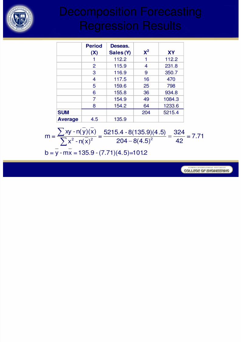
Decomposition ForecastingRegression Results
Period
(X)
Deseas.
Sales (Y) X2 XY
1 112.2 1 112.2
2 115.9 4 231.8
3 116.9 9 350.7
4 117.5 16 470
5 159.6 25 7986 155.8 36 934.8
7 154.9 49 1084.3
8 154.2 64 1233.6
SUM 204 5215.4
Average 4.5 135.9
2.101)=5(7.71)(4.-135.9=xm-y=b
7.71=42
324
)5.4(8204
.5)8(135.9)(4-5215.4=
)xn(-x
)x)(yn(-xy=m
222
Page 46
8/4/2019 Forecasting 2008
http://slidepdf.com/reader/full/forecasting-2008 46/67
Decomposition Forecast
• Regression on the de-seasonalized dataproduces the following results: – Slope (m) = 7.71 – Intercept (b) = 101.2
• Forecasts can be performed using thefollowing equation – [mx + b](seasonal factor)
Page 47
8/4/2019 Forecasting 2008
http://slidepdf.com/reader/full/forecasting-2008 47/67
0
50 100 150 200
250 300
1 2 3 4 5 6 7 8 9 10 11 12
Decomposition Forecasting
Period Quarter Sales Forecast
1 Spring 90 87.4
2 Summer 157 157.9
3 Fall 123 130.84 Winter 93 104.5
5 Spring 128 112.1
6 Summer 211 199.7
7 Fall 163 163.3
8 Winter 122 128.8
9 Spring 136.8
10 Summer 241.4
11 Fall 195.7
12 Winter 153.2
Page 48
8/4/2019 Forecasting 2008
http://slidepdf.com/reader/full/forecasting-2008 48/67
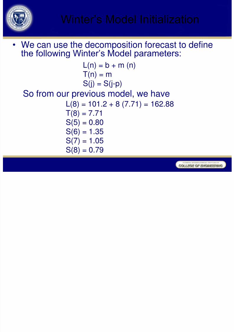
Winter‘s Model Initialization
• We can use the decomposition forecast to definethe following Winter‘s Model parameters:
L(n) = b + m (n)T(n) = m
S(j) = S(j-p)
L(8) = 101.2 + 8 (7.71) = 162.88T(8) = 7.71
S(5) = 0.80S(6) = 1.35S(7) = 1.05S(8) = 0.79
So from our previous model, we have
Page 49
8/4/2019 Forecasting 2008
http://slidepdf.com/reader/full/forecasting-2008 49/67
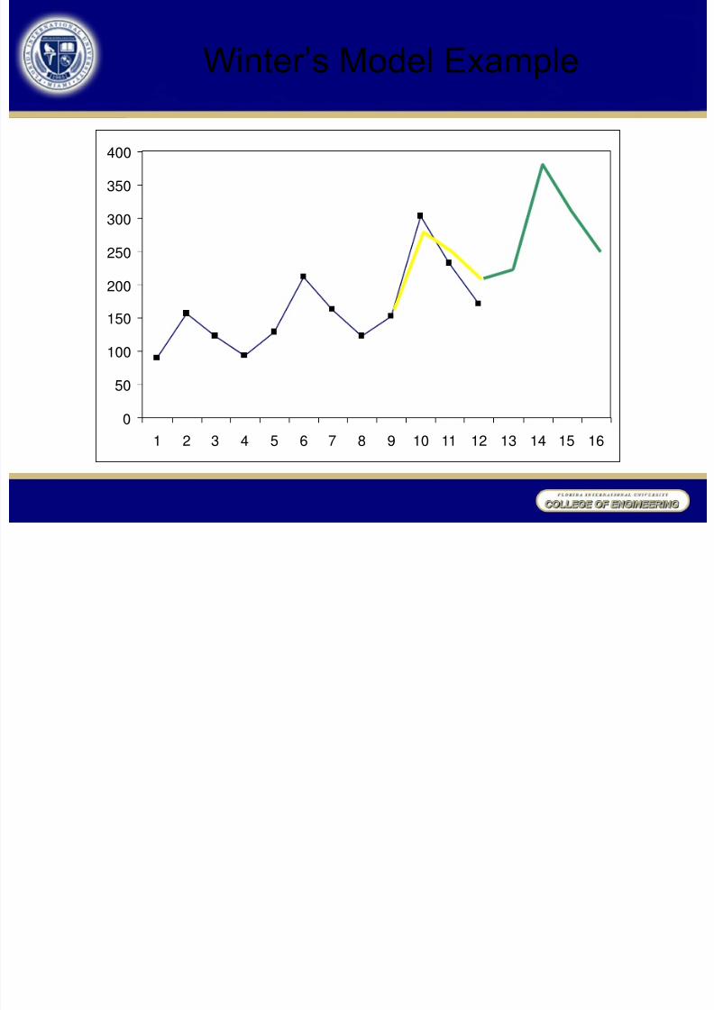
Winter‘s Model Example
176.41 10.04 0.81 136.47 197.85 14.60 1.39 251.71 215.00 15.62 1.06 223.07
9 Spring 152 10 Summer 303 11 Fall 232 12 Winter 171 226.37 13.92 0.78 182.19 13 Spring 14 Summer 15 Fall 16 Winter
195.19 352.41 283.09 220.87
= 0.3 = 0.4 g = 0.2 Period Quarter Sales L(t) T(t) S(t) F(t)
1 Spring 90 2 Summer 157 3 Fall 123 4 Winter 93 5
Spring
128
0.8
6 Summer 211 1.35 7 Fall 162 1.05 8 Winter 122 162.88 7.71 0.79
Page 50
8/4/2019 Forecasting 2008
http://slidepdf.com/reader/full/forecasting-2008 50/67
0 50
100 150 200 250 300 350 400
1 2 3 4 5 6 7 8 9 10 11 12 13 14 15 16
Winter‘s Model Example
Page 51
8/4/2019 Forecasting 2008
http://slidepdf.com/reader/full/forecasting-2008 51/67
Evaluating Forecasts
―Trust, but Verify‖ Ronald W. Reagan
• Computer software gives us the ability to mess up
more data on a greater scale more efficiently• While software like SAP can automatically selectmodels and model parameters for a set of data,and usually does so correctly, when the data is
important, a human should review the modelresults• One of the best tools is the human eye
Page 52
8/4/2019 Forecasting 2008
http://slidepdf.com/reader/full/forecasting-2008 52/67
0 10 20 30 40 50 60
1 2 3 4 5 6 7 8 9 10 11 12 13 14 15
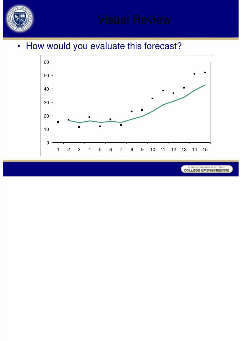
Visual Review
• How would you evaluate this forecast?
Page 53
8/4/2019 Forecasting 2008
http://slidepdf.com/reader/full/forecasting-2008 53/67
0 50
100 150 200 250 300 350 400
0 10 20 30 40 50
Forecast Evaluation
Initialization ExPostForecast
Forecast
Where Forecast is EvaluatedDo not includeinitialization datain evaluation
Page 54
8/4/2019 Forecasting 2008
http://slidepdf.com/reader/full/forecasting-2008 54/67
Page 55
8/4/2019 Forecasting 2008
http://slidepdf.com/reader/full/forecasting-2008 55/67
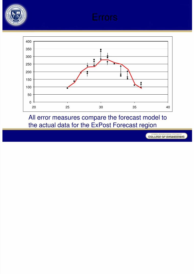
Errors Measure
All error measures are based on the comparison of forecastvalues to actual values in the ExPost Forecast region—do notinclude data from initialization.
t F(t) A(t)Error
F(t) - A(t) | F(t) - A(t) |
25 95 91 4 4
26 125 137 -12 12
27 197 193 4 4
28 227 199 28 28
29 230 278 -48 48
30 274 344 -70 70
31 274 291 -17 17
32 255 250 5 5
33 244 171 73 73
34 211 152 59 59
35 114 111 3 3
36 85 127 -42 42Sum -13 365
Page 56
8/4/2019 Forecasting 2008
http://slidepdf.com/reader/full/forecasting-2008 56/67
Bias and MAD
t F(t) A(t)Error
F(t) - A(t) | F(t) - A(t) |
25 95 91 4 4
26 125 137 -12 12
35 114 111 3 336 85 127 -42 42
Sum -13 365
08.1
12
13
n
)t( A )t(FBias
42.3012
365
n
)t( A )t(FMAD
Page 57
8/4/2019 Forecasting 2008
http://slidepdf.com/reader/full/forecasting-2008 57/67
• Bias tells us whether we have a tendency to over-or under-forecast. If our forecasts are ―in themiddle‖ of the data, then the errors should beequally positive and negative, and should sum to 0.
• MAD (Mean Absolute Deviation) is the averageerror, ignoring whether the error is positive ornegative.
• Errors are bad, and the closer to zero an error is,
the better the forecast is likely to be.• Error measures tell how well the method worked inthe ExPost forecast region. How well the forecastwill work in the future is uncertain.
Bias and MAD
Page 58
8/4/2019 Forecasting 2008
http://slidepdf.com/reader/full/forecasting-2008 58/67
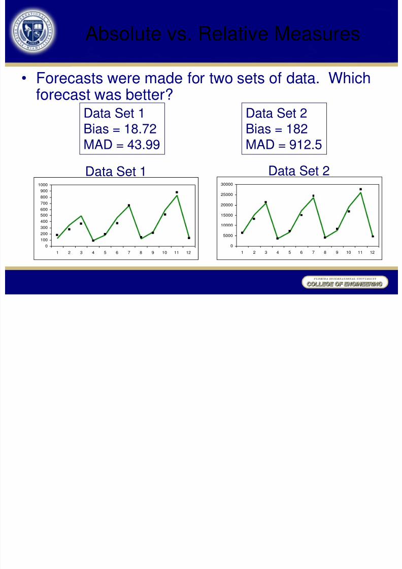
Absolute vs. Relative Measures
• Forecasts were made for two sets of data. Whichforecast was better?
Data Set 1Bias = 18.72
MAD = 43.99
Data Set 2Bias = 182
MAD = 912.5
0
100
200
300
400
500
600
700
800
900
1000
1 2 3 4 5 6 7 8 9 10 11 12
Data Set 1 Data Set 2
0
5000
10000
15000
20000
25000
30000
1 2 3 4 5 6 7 8 9 10 11 12
Page 59
8/4/2019 Forecasting 2008
http://slidepdf.com/reader/full/forecasting-2008 59/67
MPE and MAPE
• When the numbers in a data set are larger inmagnitude, then the error measures are likely tobe large as well, even though the fit might not be
as ―good‖. • Mean Percentage Error (MPE) and MeanAbsolute Percentage Error (MAPE) are relativeforms of the Bias and MAD, respectively.
• MPE and MAPE can be used to compareforecasts for different sets of data.
Page 60
8/4/2019 Forecasting 2008
http://slidepdf.com/reader/full/forecasting-2008 60/67
MPE and MAPE
• Mean Percentage Error (MPE)
n
)t( A
)t( A )t(F
MPE
n
)t( A
)t( A )t(F
MAPE
• Mean Absolute Percentage Error (MAPE)
Page 61
8/4/2019 Forecasting 2008
http://slidepdf.com/reader/full/forecasting-2008 61/67
MPE and MAPE
Data Set 1
148.012
774.1MAPE
037.012446.0MPE
t A(t) F(t)
F(t) - A(t)
A(t)
| F(t) - A(t) |
A(t)
9 177 125.4 -0.292 0.292
10 275 338.85 0.232 0.232
11 363 493.2 0.359 0.35912 91 89.1 -0.021 0.021
13 194 176 -0.093 0.093
14 376 463.05 0.232 0.232
15 659 658.8 0.000 0.000
16 146 116.7 -0.201 0.201
17 219 226.6 0.035 0.03518 514 587.25 0.143 0.143
19 875 824.4 -0.058 0.058
20 130 144.3 0.110 0.110
0.446 1.774
Page 62
8/4/2019 Forecasting 2008
http://slidepdf.com/reader/full/forecasting-2008 62/67
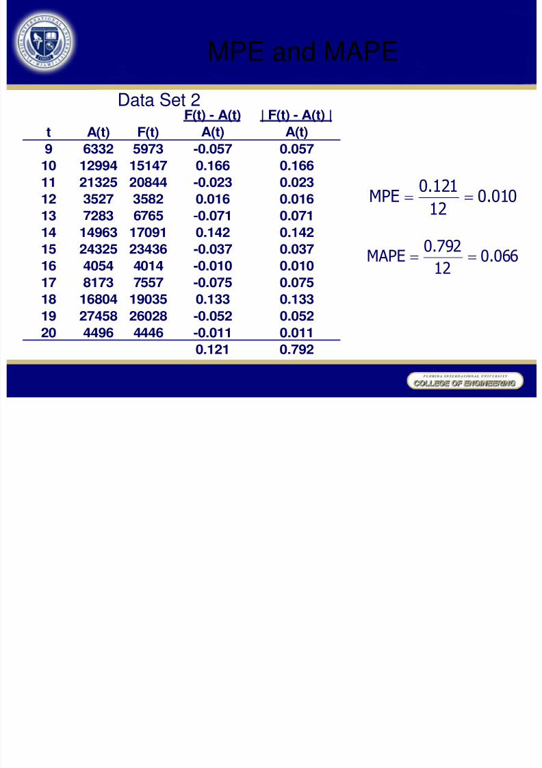
MPE and MAPE
Data Set 2
066.012
792.0MAPE
010.012121.0MPE
t A(t) F(t)
F(t) - A(t)
A(t)
| F(t) - A(t) |
A(t)
9 6332 5973 -0.057 0.057
10 12994 15147 0.166 0.166
11 21325 20844 -0.023 0.023
12 3527 3582 0.016 0.016
13 7283 6765 -0.071 0.071
14 14963 17091 0.142 0.142
15 24325 23436 -0.037 0.037
16 4054 4014 -0.010 0.010
17 8173 7557 -0.075 0.07518 16804 19035 0.133 0.133
19 27458 26028 -0.052 0.052
20 4496 4446 -0.011 0.011
0.121 0.792
Page 63
8/4/2019 Forecasting 2008
http://slidepdf.com/reader/full/forecasting-2008 63/67
MPE and MAPE
Data Set 2
066.012
792.0MAPE
010.012
121.0MPE
148.012774.1MAPE
037.012
446.0MPE
Data Set 1
0
100
200
300
400500
600
700
800
900
1000
1 2 3 4 5 6 7 8 9 10 11 12
0
5000
10000
15000
20000
25000
30000
1 2 3 4 5 6 7 8 9 10 11 12
Page 64
8/4/2019 Forecasting 2008
http://slidepdf.com/reader/full/forecasting-2008 64/67
0 10 20 30 40 50 60
1 2 3 4 5 6 7 8 9 10 11 12 13 14 15
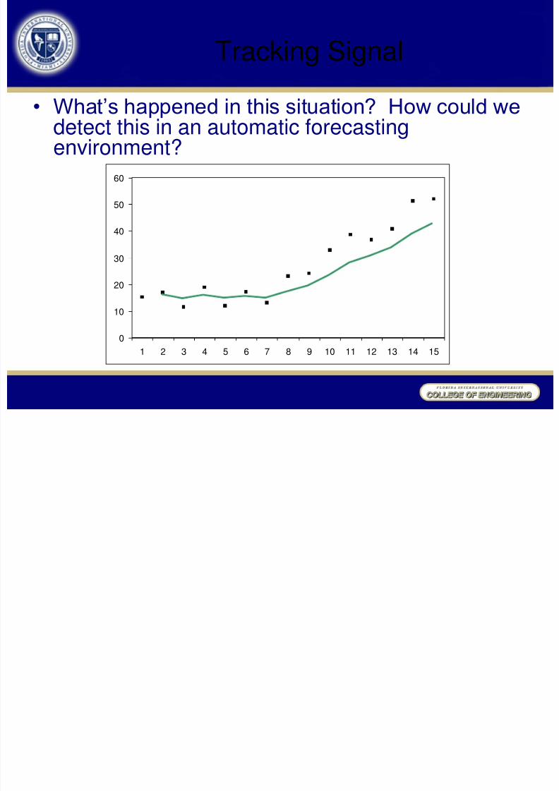
Tracking Signal
• What‘s happened in this situation? How could wedetect this in an automatic forecastingenvironment?
Page 65
8/4/2019 Forecasting 2008
http://slidepdf.com/reader/full/forecasting-2008 65/67
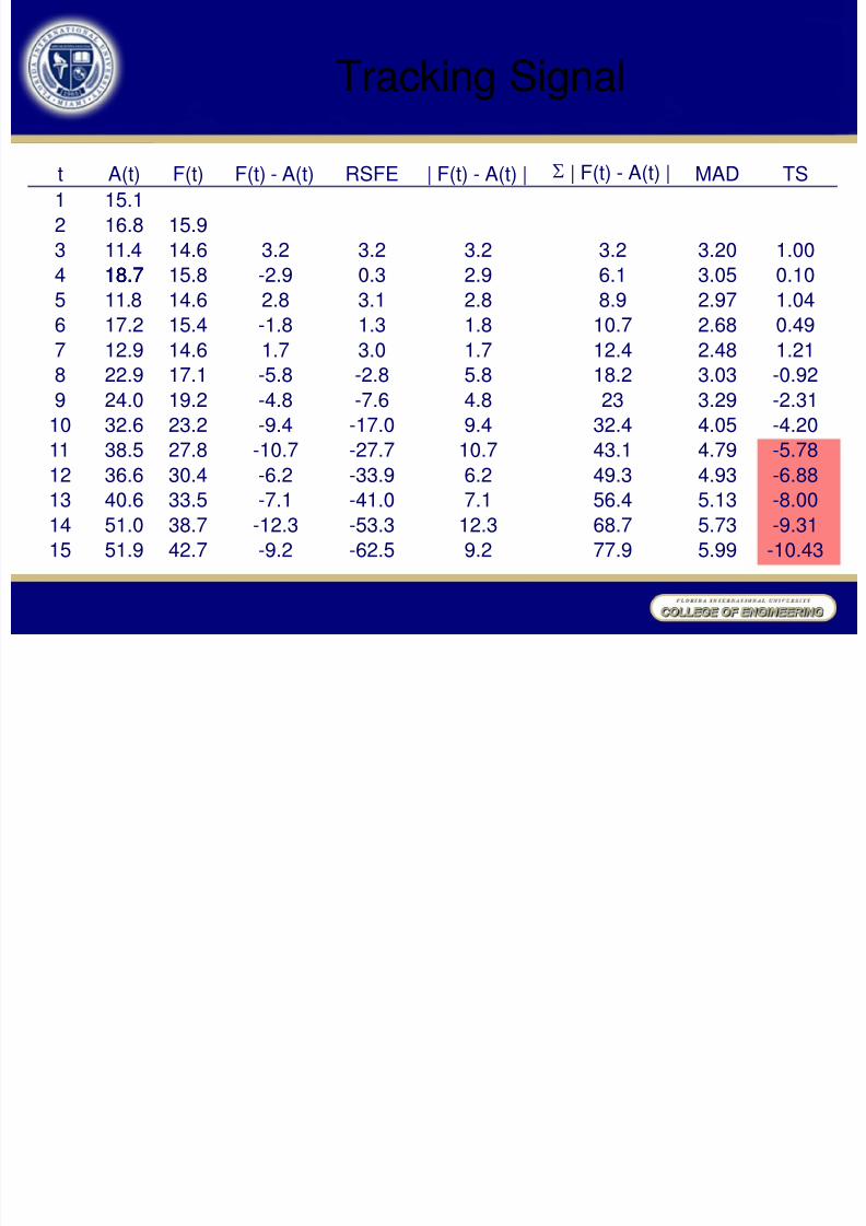
Tracking Signal
• The tracking signal can be calculated after each actualsales value is recorded. The tracking signal iscalculated as:
n
)t( A )t(F
)t( A )t(F
)t(MAD
RSFE)t(TS
• The tracking signal is a relative measure, like MPE
and MAPE, so it can be compared to a set value(typically 4 or 5) to identify when forecastingparameters and/or models need to be changed.
Page 66
8/4/2019 Forecasting 2008
http://slidepdf.com/reader/full/forecasting-2008 66/67
Tracking Signal
t A(t) F(t) F(t) - A(t) RSFE | F(t) - A(t) | S | F(t) - A(t) | MAD TS 1 15.1 2 16.8 15.9 3 11.4 14.6 3.2 3.2 3.2 3.2 3.20 1.00 4 18.7 15.8 -2.9 0.3 2.9 6.1 3.05 0.10 5
11.8
14.6
2.8
3.1
2.8
8.9
2.97
1.04
6 17.2 15.4 -1.8 1.3 1.8 10.7 2.68 0.49 7 12.9 14.6 1.7 3.0 1.7 12.4 2.48 1.21 8 22.9 17.1 -5.8 -2.8 5.8 18.2 3.03 -0.92 9 24.0 19.2 -4.8 -7.6 4.8 23 3.29 -2.31
10 32.6 23.2 -9.4 -17.0 9.4 32.4 4.05 -4.20 11
38.5
27.8
-10.7
-27.7
10.7
43.1
4.79
-5.78
12 36.6 30.4 -6.2 -33.9 6.2 49.3 4.93 -6.88 13 40.6 33.5 -7.1 -41.0 7.1 56.4 5.13 -8.00 14 51.0 38.7 -12.3 -53.3 12.3 68.7 5.73 -9.31 15 51.9 42.7 -9.2 -62.5 9.2 77.9 5.99 -10.43
18.7 18.7
Page 67
8/4/2019 Forecasting 2008
http://slidepdf.com/reader/full/forecasting-2008 67/67
0 10 20 30 40
50 60
1 2 3 4 5 6 7 8 9 10 11 12 13 14 15
Tracking Signal
TS = -5.78