FEDERAL RESERVE BANK OF SAN FRANCISCO WORKING PAPER SERIES Working Paper 2007-16 http://www.frbsf.org/publications/economics/papers/2007/wp07-16bk.pdf The views in this paper are solely the responsibility of the authors and should not be interpreted as reflecting the views of the Federal Reserve Bank of San Francisco or the Board of Governors of the Federal Reserve System. Forecasting Recessions: The Puzzle of the Enduring Power of the Yield Curve Glenn D. Rudebusch Federal Reserve Bank of San Francisco John C. Williams Federal Reserve Bank of San Francisco July 2008
Transcript
FEDERAL RESERVE BANK OF SAN FRANCISCO
WORKING PAPER SERIES
Working Paper 2007-16 http://www.frbsf.org/publications/economics/papers/2007/wp07-16bk.pdf
The views in this paper are solely the responsibility of the authors and should not be interpreted as reflecting the views of the Federal Reserve Bank of San Francisco or the Board of Governors of the Federal Reserve System.
Forecasting Recessions:
The Puzzle of the Enduring Power of the Yield Curve
Glenn D. Rudebusch Federal Reserve Bank of San Francisco
John C. Williams
Federal Reserve Bank of San Francisco
July 2008
Forecasting Recessions:
The Puzzle of the Enduring Power of the Yield Curve∗
Glenn D. Rudebusch† John C. Williams‡
July 2008
Abstract
For over two decades, researchers have provided evidence that the yield curve, specif-
ically the spread between long- and short-term interest rates, contains useful infor-
mation for signaling future recessions. Despite these findings, forecasters appear to
have generally placed too little weight on the yield spread when projecting declines in
the aggregate economy. Indeed, we show that professional forecasters appear worse
at predicting recessions a few quarters ahead than a simple real-time forecasting
model that is based on the yield spread. This relative forecast power of the yield
curve remains a puzzle.
Keywords: yield spread, probability forecasts, real-time
∗For helpful comments, we thank Boragan Aruoba, Frank Diebold, Arturo Estrella, Oscar Jorda, participantsat the conference on real-time data analysis held at the Federal Reserve Bank of Philadelphia in 2007, our JBESEditor and Associate Editor, and two anonymous referees. Wayne Huang, Vuong Nguyen, Anjali Upadhyay, andStephanie Wang provided excellent research assistance. The views expressed in this paper are our own and notnecessarily those of others at the Federal Reserve Bank of San Francisco.†Federal Reserve Bank of San Francisco; www.frbsf.org/economists/grudebusch; [email protected].‡Federal Reserve Bank of San Francisco; [email protected].
1
First on Monday and then again on Thursday, [former Fed Chairman] Greenspan upset stockmarkets merely by uttering the word “recession” and saying that one might but probably wouldnot occur by the end of this year. . . . Mr. Greenspan’s use of the R-word helped push down theDow Jones industrial average by about 200 points on Thursday morning.
— The New York Times, March 2, 2007
1 Introduction
The word “recession” conjures a variety of fears—for workers who suffer job losses, for investors
who endure asset price declines, for entrepreneurs who risk bankruptcy. Recessions are periods
of greater dislocation and anxiety, higher unemployment and suicide rates, and lower output and
profits. In the United States, recessions have become less frequent and less severe in the past two
decades; however, nonrecessionary episodes have also become more stable, so in relative terms,
as the market sensitivity in the epigraph suggests, recessions appear to many to be as perilous
as before. Therefore, any ability to predict recessions remains highly profitable to investors and
very useful to policymakers and other economic agents. Accordingly, there remains a keen and
widespread interest in predicting recessions, and our paper examines what economic forecasters
know about the likely occurrence of a recession and, most importantly, when do they know it.
Our analysis focuses on two divergent strands in the recession prediction literature. First,
it is common wisdom that economists are not very good at forecasting recessions. For example,
Zarnowitz and Braun (1993) showed that economic forecasters made their largest prediction
errors during recessions, and Diebold and Rudebusch (1989, 1991a,b) reach a pessimistic as-
sessment of the ability of the well-known index of leading indicators to provide useful signals of
future recessions. The second strand of the literature comes to a very different conclusion about
the predictability of recessions, namely, that the slope of the yield curve, that is, the spread
between long- and short-term interest rates, is useful in forecasting real gross domestic product
(GDP) growth and recessions. The predictive power of the yield spread for real activity was
demonstrated by Harvey (1989), Stock and Watson (1989), and Estrella and Hardouvelis (1991).
The ability of the yield spread to predict recessions has been most recently described by Dotsey
(1998), Estrella and Mishkin (1998), Estrella (2005), Chauvet and Potter (2005), Ang, Piazzesi,
and Wei (2006), and Wright (2006).
In this paper, we examine the apparent contradiction between these two strands of the reces-
1
sion prediction literature. We provide new evidence on this issue by examining the information
content of probability forecasts provided by participants in the Survey of Professional Forecast-
ers (SPF) and compare these forecasts to real-time recession predictions based on the yield curve
spread. As discussed in Croushore (1993), SPF forecasts of GDP growth and inflation have been
found to perform well in forecast evaluation exercises. The SPF also asks panelists to estimate
the probabilities that real GDP will decline in the quarter in which the survey is taken and
in each of the following four quarters. These data have two advantages as real-time recession
forecasts. First, unlike other surveys that occasionally ask questions on recession probabilities
(e.g., the Blue Chip survey), the SPF has asked these questions each quarter for nearly 40 years,
providing a long time series of real-time recession forecasts. Second, these forecasts should incor-
porate all information available to professional forecasters and therefore provide better forecasts
of recessions than implied by the leading indicators and other forecasting methods that have
been found wanting in past forecast evaluations. Indeed, Lahiri and Wang (2006) analyzed the
forecast performance of the SPF probability forecasts for the current and the next quarter and
found them to contain predictive power. But, those authors did not compare these forecasts to
those from other models or look at forecast horizons beyond one quarter.
We find that the SPF probability forecasts are somewhat better at forecasting recessions in
the current quarter than forecasts from a simple probit model using the yield spread; however,
this difference is not statistically significant at the 5% level. Moreover, the SPF’s relative
predictive power deteriorates at forecast horizons of one quarter or more. These findings are
robust to alternative measures of forecast performance. Evidently, the pessimistic assessment of
the ability of economists to forecast recessions holds for the SPF probability forecasts as well.
The forecasts from the yield spread model, based on real-time estimates, are significantly
more accurate than the SPF probability forecasts for forecast horizons of three and four quarters.
At shorter horizons, the yield curve spread model is not useful at predicting recessions and its
forecast accuracy is statistically indistinguishable from those of the SPF. This finding that
the simple yield curve spread model dominates the SPF at longer horizons is a puzzle for the
hypothesis that forecasters incorporate all available information (as discussed by Fernald and
Trehan 2006). We show that SPF forecasts of real GDP growth exhibit the same pattern, with
forecast errors highly correlated with the lagged yield spread.
We find that the puzzling dominance of the yield curve model over the SPF forecasts has
2
endured, suggesting that economists in the survey failed to “learn” about the usefulness of
the yield spread for forecasting recessions. In particular, the yield curve model dominates the
SPF forecasts in a sample covering only the past 20 years. This finding is especially puzzling,
because the usefulness of the yield curve spread to predict output growth and recessions received
widespread attention among economists in the late 1980s. Indeed, in our analysis, we use a very
simple real-time model identical to that proposed by Estrella and Hardouvelis (1991), which
practitioners should have been aware of for most of the past 20 years. The simple yield curve
model still dominates the SPF forecasts at horizons of three and four quarters in most cases for
this shorter sample. Even after the predictive power of the yield curve had been well publicized,
it appears that SPF participants did not incorporate all of the available yield curve information
into their forecasts of economic activity.
The paper proceeds as follows. In the next section, we provide a simple definition of recessions
in terms of real GDP growth. In Section 3, we describe a variety of alternative real-time
probability forecasts for these GDP-based recessions. In Section 4, we assess the accuracy of
these forecasts. In Section 5, we examine whether the evidence on the relative forecast accuracy
has changed over time, and we conclude with some speculation about possible resolutions to the
puzzle of the enduring relative power of the yield curve for predicting recessions.
2 Defining Recessions
As a first step, it is necessary to define what constitutes a “recession.” The National Bureau of
Economic Research (NBER), which has been dating recessions for almost 80 years, provides the
most widely accepted definition of a recession (NBER 2003):
A recession is a significant decline in economic activity spread across the economy,lasting more than a few months, normally visible in real GDP, real income, employ-ment, industrial production, and wholesale-retail sales. A recession begins just afterthe economy reaches a peak of activity and ends as the economy reaches its trough.Between trough and peak, the economy is in an expansion.
Thus, in determining the dates of business cycle peaks and troughs, the NBER does not rely on
any single macroeconomic indicator, but instead examines a large collection of variables. These
individual series have idiosyncratic movements but also display substantial comovement and
correlation, and the NBER selects the overall business cycle peak and trough months to best
capture the general consensus among the various series of the high and low points in economic
3
activity. For detailed discussion of the NBER methodology, see Diebold and Rudebusch (1992,
1996). Based on this methodology, the NBER publishes a historical chronology of the monthly
dates of past business cycle peaks and troughs, which delineate recessions and expansions. (For
a modern dynamic factor approach for measuring economic activity, see Aruoba, Diebold, and
Scotti, 2008.)
The NBER business cycle dating methodology requires substantial judgment in its applica-
tion, and the resulting chronology is not without measurement error. Diebold and Rudebusch
(1992) describe some of the uncertainty about the precise monthly dating of the general turns in
business activity; however, even if one accepts the NBER dates of cyclical peaks and troughs as
stated, there remains some ambiguity about when a recession starts and ends. Specifically, the
peak and trough months could be classified as the first month of a recession and the first month
of an expansion, respectively, or as the last month of an expansion and the last month of a re-
cession, respectively. The latter convention, in which the recession starts in the month following
the peak month and ends on the date of the subsequent trough month, is the more common one
(e.g., Diebold and Rudebusch 1989). (In contrast, the NBER’s view is that the day when the
economy turns around is contained within the peak or trough month, so those months are blends
of both recession and expansion phases.) A further complication arises from the translation
of the monthly dates into designations of peaks and troughs at a quarterly frequency, which
we employ in our analysis because the SPF is quarterly. Such a translation can be done in a
variety of ways, and we follow the most common convention (e.g., Estrella and Trubin 2006)
and assume that a recession starts in the quarter that directly follows the quarter containing
the peak month and that it ends in the quarter containing the trough month. Our resulting
chronology of quarterly NBER recessions and expansions is represented by a binary variable,
with a one for a recession quarter and a zero otherwise, which will be denoted as RNBERt. See
the web appendix to this article for further details of this variable. We also obtained similar
dating of recessions using an alternative convention in which a recession quarter was defined to
contain two or more recession months or using the convention in Wright (2006), in which both
the peak quarter and trough quarter were counted as recession quarters, but we do not report
those results here.
For our analysis, we employ a simple rule that links declines in real GDP to recessions.
As noted by the NBER (2003): “The NBER considers real GDP to be the single measure
4
that comes closest to capturing what it means by ‘aggregate economic activity.’ The [NBER]
therefore places considerable weight on real GDP and other output measures.” Of course, as in
any real-time analysis, the issue of which vintage of data to use is important, and we consider
three different data series for real GDP growth. The first series is the so-called “first-final”
data which is released about three months after the end of each quarter. This is our preferred
real-time measure of GDP. It incorporates a great deal of information about expenditures and
is a reasonably accurate measure of GDP based on the methodology in place at the time. The
second is the latest revised estimates available as of February 2007. These data have been subject
to multiple revisions and, importantly, incorporate significant changes in methodology, making
comparison of real-time forecasts to revised data problematic. The third is the “advance” data,
which is released about one month after the end of the quarter. At the time of publication of
these data, several important source data are still unavailable, making these estimates subject to
greater measurement error than the “first-final” estimates. See the web appendix to this article
for further details on these data.
A straightforward rule for defining recessions that works quite well is what we dub the
“R1 rule,” which simply defines any single quarter of negative real GDP growth as a recession
quarter. The associated binary variable of recession quarters is denoted as R1t. A value of one
indicates that the growth rate of real GDP was negative in that quarter, otherwise the value
is zero. Applied to first-final data, the R1 rule produces 14 recession quarters that match one
of the 21 NBER recession quarters, with only seven missed calls of recession. The R1 rule also
produces five false calls of recession (including one by a whisker in 1978:Q1). Therefore, there
are 12 total quarters of incorrect signals and the mix of missed calls is reasonably balanced. The
R1 rule has advantages in terms of simplicity and its direct connection to the survey questions
in the SPF (described below), and we therefore use it for our analysis for the remainder of the
paper.
For comparison, we also consider the recession dates that one obtains by applying what we
call the “R2 rule,” which defines a recession as occurring if there are two consecutive quarters of
negative real GDP growth. In particular, we say that a quarter is in an R2 recession if real GDP
falls in that quarter and if either (or both) the previous and following quarters post negative
real GDP growth as well. This definition of a recession is often mentioned in the media, but in
practice, it performs rather poorly as a proxy for NBER recession dates. Using any of the three
5
vintages of data, the R2 rule appears too stringent a criterion to provide a good match to the
NBER business-cycle dating methodology. For example, applying the R2 rule to the first-final
data produces only ten recession quarters that match one of the 21 NBER recession quarters,
with 11 quarters of missed recession signals. Perhaps most problematic, the R2 rule using the
first-final data completely misses the 1980 and 2001 NBER recessions. The R2 rule produces
only two false calls of recession quarters relative to the NBER definition (in 1969 and 1991).
Overall then, the R2 rule gives a total of 13 quarters of incorrect recession signals. See the web
appendix to this article for detailed R1 and R2 chronologies.
3 Recession Probability Forecasts
In this section, we describe various alternative real-time probability forecasts of R1 recession
quarters using the first-final data. These are based on information from the SPF or from a
probit model using the yield curve slope as an explanatory variable. In the next section, we will
provide a formal statistical examination of their relative accuracy.
3.1 SPF reported probability forecasts
Every quarter since the fourth quarter of 1968, the SPF has asked its participants to provide
estimates of the probability of negative real GDP growth in that quarter as well as probabilities
of negative growth in the current quarter and each of the next four quarters. The survey typically
was due by the middle of the second month of the quarter (in recent years, the due date has
been moved up a week, to around the 7th of the second month of the quarter). The number
of respondents has varied over time, with a median of about 34. For a detailed discussion of
the SPF, see Croushore (1993). There are four missing observations for the four-quarter-ahead
probability forecasts, with the final one occurring during the survey taken in the third quarter
of 1974. Because we allow for autocorrelation of residuals in the computation of standard errors
for our forecast accuracy statistics, the missing observations would require us to drop six years of
data from our sample. Instead, we replaced the missing observations on the four-quarter-ahead
probability forecasts with the three-quarter-ahead probability forecasts from the same survey.
Our main results also hold if we simply drop the six years of data for the four-quarter-ahead
forecasts.
6
The wording of the specific survey question is very clear and has changed little over time,
and in 2007 it read as follows:
Indicate the probability you would attach to a decline in real GDP (chain-weightedbasis, seasonally adjusted) in the next five quarters. Write in a figure that may rangefrom 0 to 100 in each of the cells (100 means a decline in the given quarter is certain,i.e. 100 percent, 0 means there is no chance at all, i.e. 0 percent).
The mean probability forecast for quarter t that was reported in response to this question asked
in the survey in quarter t− h is denoted PSPFt|t−h.
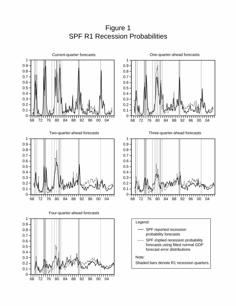
Importantly, these are direct real-time probability forecasts of what we have termed R1
recessions that require no ex post adjustments or filtering. The solid lines in the five panels of
Figure 1 plot these probabilities for the current quarter (h = 0) and for the future four quarters.
(Note that in each panel PSPFt|t−h is plotted in quarter t, regardless of the value of the forecast
horizon h.)
For forecasting the current quarter, the SPF participants appear to be able to delineate
periods of weak or negative real GDP growth. However, the SPF predictive information re-
garding R1 recessions quickly erodes as the forecast horizon increases. Certainly for three-
and four-quarter-ahead forecasts, it does not appear that the SPF forecasts have much, if any,
information.
3.2 SPF implied probability forecasts
Our second sequence of recession probability forecasts is derived from the real output forecasts
reported in the SPF. We use this measure primarily as a check to see whether the SPF proba-
bility forecasts are consistent with the SPF real GDP forecasts. We use the median real GDP
forecasts for quarter t from the SPF in quarter t − h and the historical error variances associ-
ated with forecasts at various horizons to compute implied recession probabilities PGDPt|t−h . For
the purpose of constructing the SPF implied probability forecasts, we have replaced the four
missing observations for the four-quarter-ahead real GDP forecasts (mentioned above) with the
corresponding three-quarter-ahead forecasts. Excluding these data entirely from the analysis
does not affect our results.
Unfortunately, we do not have real-time data on the distributions forecasters placed around
their output forecasts. Moreover, we do not have SPF forecasts prior to the fourth quarter of
1968 that we could use to construct estimates of such distributions based on past forecast errors.
7
Instead, we assume that the distributions around the forecasts follow the normal distribution,
with variances set equal to the full-sample variances of SPF real GDP growth forecast errors for
each forecast horizon. (There are four missing observations for the four-quarter-ahead real GDP
forecasts, with the final one occurring in the first quarter of 1970. These are dropped from the
sample in computing the forecast error variances.) Note that because we apply the same forecast
error variances to all forecast vintages, these are not true real-time recession probabilities in that
they are computed as if forecasters knew the full-sample variances of forecast errors. Still, these
probabilities are based on the real-time GDP point forecasts. The resulting forecasts are shown
by the dashed lines in Figure 1.
The differences between the reported SPF recession probabilities and the implied probabili-
ties based on the GDP forecasts are generally small and fairly uniform over time, which suggests
that the SPF participants provide GDP point forecasts that are fairly consistent with their re-
ported negative growth probability forecasts. This helps validate the probability forecasts as
serious predictions. Furthermore, it suggests that there has been little change in the perceived
forecast error volatility over time. Recall that the implied probabilities assume a constant fore-
cast error variance, which is set to its average over the full sample. This appears to be a pretty
good estimate. Notably, the differences between the reported and implied probabilities show no
clear trend and are not significantly larger or smaller at the beginning or end of the sample. This
lack of trend in the conditional volatility may appear a little surprising but is not inconsistent
with the well-known “Great Moderation” in the unconditional volatility of real GDP growth
over this period (see Campbell, 2007, and Tulip, 2005, for further discussion). Finally, a com-
parison of the two time series shows some interesting episodes. In particular, in 1979 and 1980,
which was a period of relatively high reported and implied probabilities of negative growth, the
SPF participants underestimated that likelihood relative to what was implied by their GDP
forecasts. Similarly, during much of the 1990s, the reported probabilities were lower than would
be expected based on the GDP forecasts and historical forecast error distributions.
3.3 Yield-curve probability forecasts
We now consider forecasts of an R1 recession that are based on the yield spread. Following
Estrella and Hardouvelis (1991), we define the yield spread, St, to be the difference between
the yield on a 10-year U.S. Treasury note, iLt , and the yield on a 3-month Treasury bill, iSt :
8
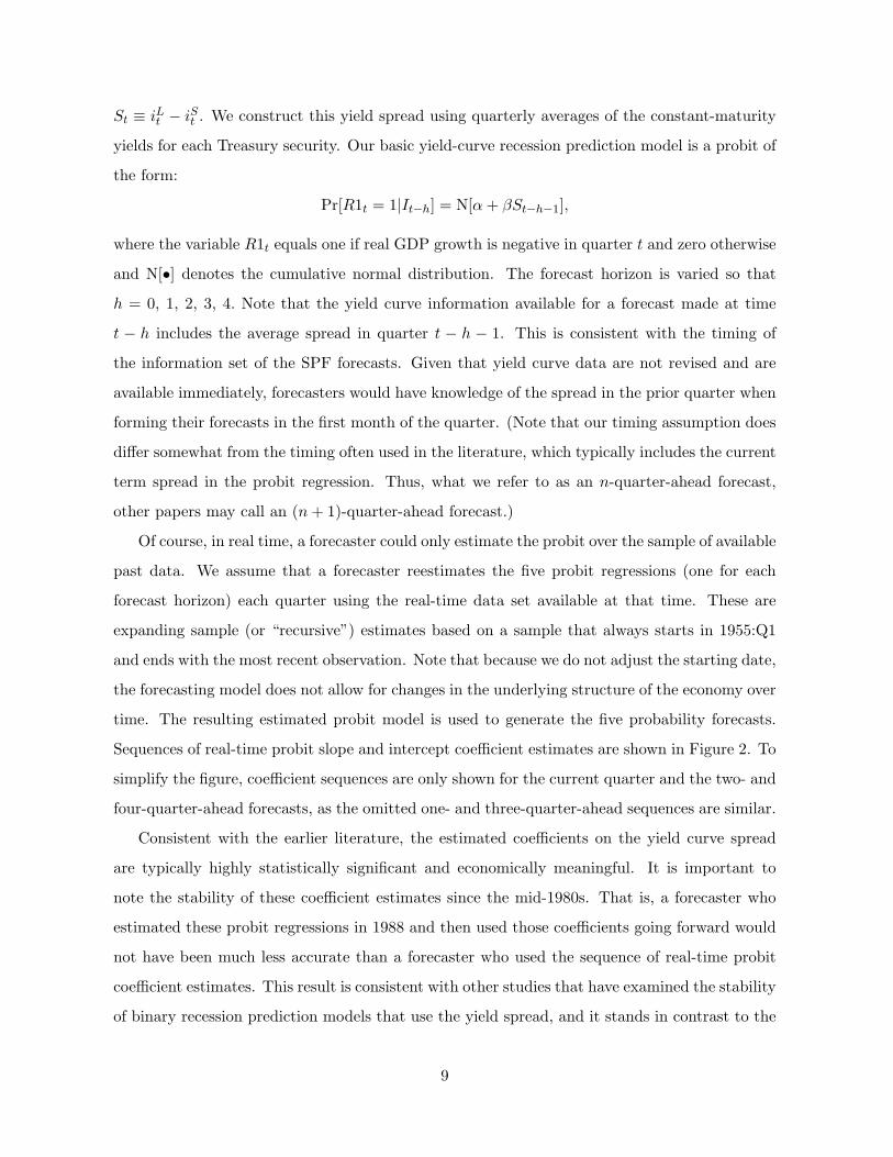
St ≡ iLt − iSt . We construct this yield spread using quarterly averages of the constant-maturity
yields for each Treasury security. Our basic yield-curve recession prediction model is a probit of
the form:
Pr[R1t = 1|It−h] = N[α+ βSt−h−1],
where the variable R1t equals one if real GDP growth is negative in quarter t and zero otherwise
and N[•] denotes the cumulative normal distribution. The forecast horizon is varied so that
h = 0, 1, 2, 3, 4. Note that the yield curve information available for a forecast made at time
t − h includes the average spread in quarter t − h − 1. This is consistent with the timing of
the information set of the SPF forecasts. Given that yield curve data are not revised and are
available immediately, forecasters would have knowledge of the spread in the prior quarter when
forming their forecasts in the first month of the quarter. (Note that our timing assumption does
differ somewhat from the timing often used in the literature, which typically includes the current
term spread in the probit regression. Thus, what we refer to as an n-quarter-ahead forecast,
other papers may call an (n+ 1)-quarter-ahead forecast.)
Of course, in real time, a forecaster could only estimate the probit over the sample of available
past data. We assume that a forecaster reestimates the five probit regressions (one for each
forecast horizon) each quarter using the real-time data set available at that time. These are
expanding sample (or “recursive”) estimates based on a sample that always starts in 1955:Q1
and ends with the most recent observation. Note that because we do not adjust the starting date,
the forecasting model does not allow for changes in the underlying structure of the economy over
time. The resulting estimated probit model is used to generate the five probability forecasts.
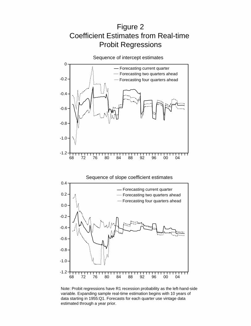
Sequences of real-time probit slope and intercept coefficient estimates are shown in Figure 2. To
simplify the figure, coefficient sequences are only shown for the current quarter and the two- and
four-quarter-ahead forecasts, as the omitted one- and three-quarter-ahead sequences are similar.
Consistent with the earlier literature, the estimated coefficients on the yield curve spread
are typically highly statistically significant and economically meaningful. It is important to
note the stability of these coefficient estimates since the mid-1980s. That is, a forecaster who
estimated these probit regressions in 1988 and then used those coefficients going forward would
not have been much less accurate than a forecaster who used the sequence of real-time probit
coefficient estimates. This result is consistent with other studies that have examined the stability
of binary recession prediction models that use the yield spread, and it stands in contrast to the
9
documented instability of (continuous) output growth prediction regressions that use the yield
spread (see Estrella, Rodrigues, and Schich 2003). This later result helps motivate our focus on
recession prediction rather than output growth prediction.
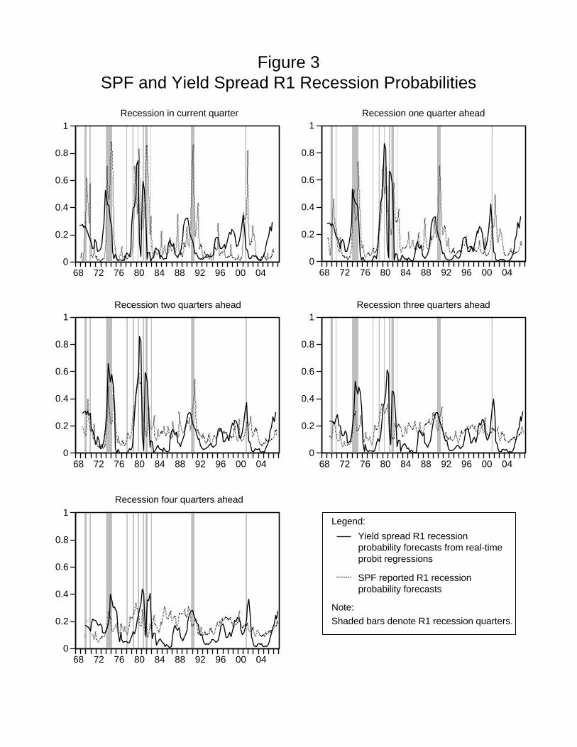
Given the real-time coefficient estimates, we define the real-time yield spread R1 recession
probability forecast as
P Y St|t−h = N[α̂t−h + β̂t−hSt−h−1],
where α̂t−h and β̂t−h are taken from the sequences of real-time estimates. The resulting yield
spread recession probability forecasts—based on real-time yield spread data and real-time probit
estimates—are shown as solid lines in Figure 3, with the SPF reported probability forecasts
repeated as the dotted line. (Again, the timing of this display plots P Y St|t−h in quarter t.)
A striking result is that the yield curve model appears to do a better job than the SPF
probability forecast at predicting when the economy is not going to be in recession for horizons
of one or more quarters. At short horizons of zero and one quarter, the SPF forecasts appear
to do better at forecasting recessions, while at horizons of three and four quarters, the yield
curve model appears to perform better. An explanation for this pattern of predictive power
of the yield spread is that the yield spread encapsulates the stance of monetary policy, which
affects the economy with a lag of a few quarters. For example, a tightening of monetary policy,
say to slow growth and inflation during an economic expansion, typically causes short rates to
rise above long rates. As a result, the yield curve model predicts a heightened probability of
recession. If the economy actually enters into a recession, the stance of monetary policy may
loosen, causing the yield curve to predict expansion just as the economy has entered into a
recession. Thus, for short forecast horizons, the data provide mixed signals, with the occurrence
of recessions sometimes being contemporaneously associated with loose monetary policy and
other times with tight monetary policy. We now turn to a formal evaluation of the relative
forecast accuracy of these two sets of forecasts.
4 Assessing Probability Forecasts
We do not know the objective that SPF participants used in deriving their forecasts. Therefore,
in assessing the relative accuracy of the SPF forecasts, we consider several alternative objectives.
In particular, we evaluate the forecasts using both the “first-final” and the “advance” GDP
releases. Although the former arguably provides a more accurate measure of economic activity,
10
economic forecasters may have been aiming to match the advance release which they (and their
clients) will see first.
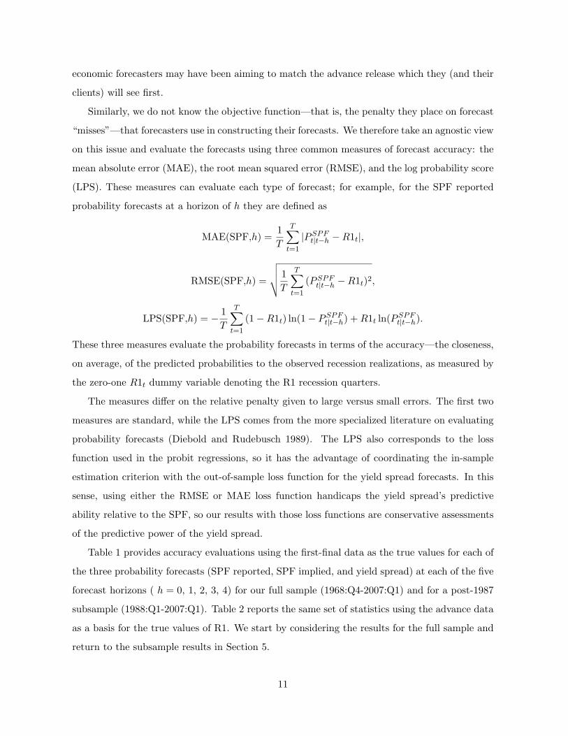
Similarly, we do not know the objective function—that is, the penalty they place on forecast
“misses”—that forecasters use in constructing their forecasts. We therefore take an agnostic view
on this issue and evaluate the forecasts using three common measures of forecast accuracy: the
mean absolute error (MAE), the root mean squared error (RMSE), and the log probability score
(LPS). These measures can evaluate each type of forecast; for example, for the SPF reported
probability forecasts at a horizon of h they are defined as
MAE(SPF,h) =1T
T∑t=1
|PSPFt|t−h −R1t|,
RMSE(SPF,h) =
√√√√ 1T
T∑t=1
(PSPFt|t−h −R1t)2,
LPS(SPF,h) = − 1T
T∑t=1
(1−R1t) ln(1− PSPFt|t−h) +R1t ln(PSPF
t|t−h).
These three measures evaluate the probability forecasts in terms of the accuracy—the closeness,
on average, of the predicted probabilities to the observed recession realizations, as measured by
the zero-one R1t dummy variable denoting the R1 recession quarters.
The measures differ on the relative penalty given to large versus small errors. The first two
measures are standard, while the LPS comes from the more specialized literature on evaluating
probability forecasts (Diebold and Rudebusch 1989). The LPS also corresponds to the loss
function used in the probit regressions, so it has the advantage of coordinating the in-sample
estimation criterion with the out-of-sample loss function for the yield spread forecasts. In this
sense, using either the RMSE or MAE loss function handicaps the yield spread’s predictive
ability relative to the SPF, so our results with those loss functions are conservative assessments
of the predictive power of the yield spread.
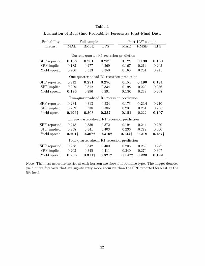
Table 1 provides accuracy evaluations using the first-final data as the true values for each of
the three probability forecasts (SPF reported, SPF implied, and yield spread) at each of the five
forecast horizons ( h = 0, 1, 2, 3, 4) for our full sample (1968:Q4-2007:Q1) and for a post-1987
subsample (1988:Q1-2007:Q1). Table 2 reports the same set of statistics using the advance data
as a basis for the true values of R1. We start by considering the results for the full sample and
return to the subsample results in Section 5.
11
4.1 Comparing SPF and yield curve probability forecasts
For the full sample of current-quarter forecasts, the SPF forecast yields smaller forecast errors
than the yield spread forecast based on both the first-final and advance data for all three mea-
sures (MAE, RMSE, and LPS). For the one-quarter-ahead forecast, the evidence is mixed as
to the relative performance of the two forecasts, with the SPF slightly more accurate in four
out of six cases based on first-final data, and in only one of six cases using advance data. For
forecast horizons of two or more quarters, however, the yield spread forecasts are consistently
more accurate than the SPF, based on all three criteria and both data series for R1 (with only
one exception out of 36 cases).
To examine the statistical significance of these differences, we apply the Diebold-Mariano
(1995) test of relative forecast accuracy. This test is based on the mean accuracy differential (or,
more generally, the loss differential) between the two forecasts. In particular, the loss differential
at a horizon h for the three accuracy measures are
Difft(MAE) = |PSPFt|t−h −R1t| − |P Y S
t|t−h −R1t|,
Difft(MSE) = (PSPFt|t−h −R1t)2 − (P Y S
t|t−h −R1t)2,
Difft(LPS) = (1−R1t)(ln(1− PSPFt|t−h)− ln(1− P Y S
t|t−h)) +R1t(ln(PSPFt|t−h)− ln(P Y S
t|t−h)).
The Diebold-Mariano (DM) test can be simply based on the t-statistic for the hypothesis of a
zero population mean differential, taking into account the fact that the differential time series
is not necessarily white noise. (The DM test is not available for an RMSE loss function, so we
report the results from the MSE version of the test.) Thus, we compute the DM test by regressing
each differential time series on an intercept and testing the significance of that intercept using
HAC standard errors, which correct for possible heteroskedasticity and autocorrelation in the
residuals.
There are two complications involved in evaluating the distribution of any DM test statistic.
First, it is important to consider potential finite sample size distortions, especially in small sam-
ples. Ideally, we would conduct a monte carlo experiment tailored to the specific circumstances
of our application in order to help guide inference. However, the absence of a model underly-
ing the SPF probability forecasts precludes use of such a tool. Instead, we employ the Kiefer,
Vogelsang, and Bunzel (2000) method for computing the HAC standard errors. As noted by
Kiefer and Vogelsang (2002), this method is equivalent to using the usual Bartlett kernel of the
12
Newy-West HAC standard error but without truncation (together with the use of nonstandard
asymptotic critical values). Importantly, Christensen, et al. (2008) find that, in the DM test
context, this method has much better finite sample size properties than other robust estima-
tors. Second, in assessing the distribution of the DM test, the issue of accounting for parameter
estimation error also arises, as discussed in detail by Corradi and Swanson (2006). Again, our
use of non-model-based judgmental SPF forecasts essentially removes such errors as a subject
of analysis. In the case of the yield spread probit forecasts, West (1996) shows that when the
in-sample objective function is the same as the out-of-sample loss function, which is true for the
LPS loss function, parameter estimation error vanishes.
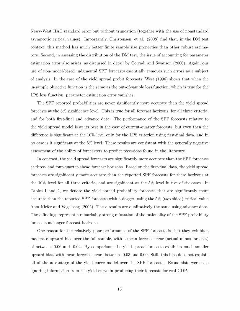
The SPF reported probabilities are never significantly more accurate than the yield spread
forecasts at the 5% significance level. This is true for all forecast horizons, for all three criteria,
and for both first-final and advance data. The performance of the SPF forecasts relative to
the yield spread model is at its best in the case of current-quarter forecasts, but even then the
difference is significant at the 10% level only for the LPS criterion using first-final data, and in
no case is it significant at the 5% level. These results are consistent with the generally negative
assessment of the ability of forecasters to predict recessions found in the literature.
In contrast, the yield spread forecasts are significantly more accurate than the SPF forecasts
at three- and four-quarter-ahead forecast horizons. Based on the first-final data, the yield spread
forecasts are significantly more accurate than the reported SPF forecasts for these horizons at
the 10% level for all three criteria, and are significant at the 5% level in five of six cases. In
Tables 1 and 2, we denote the yield spread probability forecasts that are significantly more
accurate than the reported SPF forecasts with a dagger, using the 5% (two-sided) critical value
from Kiefer and Vogelsang (2002). These results are qualitatively the same using advance data.
These findings represent a remarkably strong refutation of the rationality of the SPF probability
forecasts at longer forecast horizons.
One reason for the relatively poor performance of the SPF forecasts is that they exhibit a
moderate upward bias over the full sample, with a mean forecast error (actual minus forecast)
of between -0.06 and -0.04. By comparison, the yield spread forecasts exhibit a much smaller
upward bias, with mean forecast errors between -0.03 and 0.00. Still, this bias does not explain
all of the advantage of the yield curve model over the SPF forecasts. Economists were also
ignoring information from the yield curve in producing their forecasts for real GDP.
13
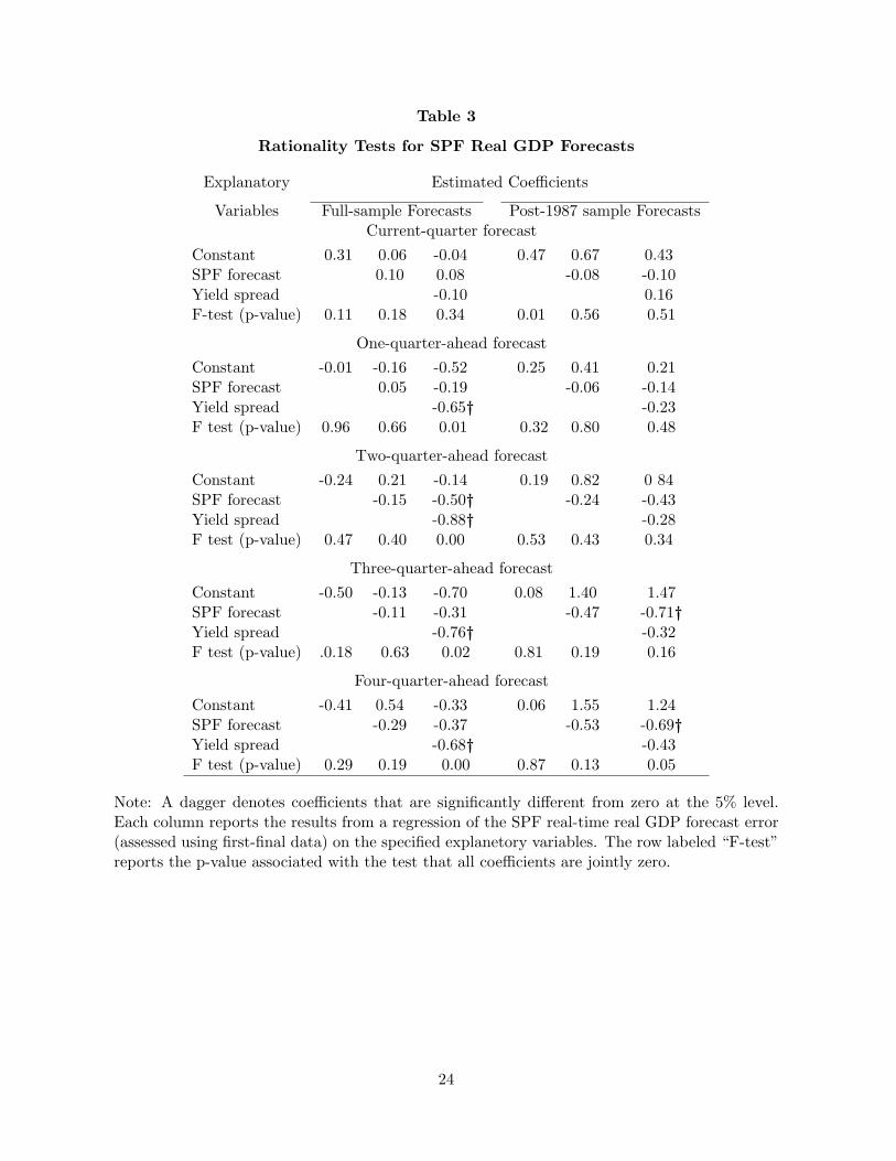
The finding that forecasters have not efficiently used all available information is also apparent
from the results of standard rationality tests of the SPF real GDP forecasts, which are reported
in Table 3. (These tests as well as more comprehensive ones are described in Corradi, Fernandez,
and Swanson, in press.) Estimated coefficients that are statistically significant at the 5% level
are indicated with a dagger. For these tests, we use Newey-West HAC standard errors with four
lags. The dependent variable is the forecast error using first-final data. (For the four-quarter-
ahead forecasts, we dropped the data before 1970:Q2 because of missing observations in some
of those quarters.) The first two columns of the table report results from standard rationality
tests. As shown in the first column of the table, over the full sample, the mean GDP forecast
errors are not significantly different from zero. The second column shows that the GDP forecast
errors are not correlated with the SPF forecasts. Thus, these two commonly used measures
suggest that SPF GDP forecasts are rational. However, as seen in the third column of the table,
the forecast errors are significantly correlated with the lagged yield curve spread for forecast
horizons of one or more quarters, indicating that the SPF GDP forecasts suffer from the same
problem as the SPF recession forecasts. Evidently, forecasters either did not know about the
predictive power of the yield curve or failed to use this knowledge effectively in the past. We
return to this issue in the next section.
One potential explanation for the weak performance of the SPF forecasts is our choice of
accuracy measures. It could be the case that forecasters use a very different loss function in
preparing their probability forecasts, and other measures of forecast accuracy could give different
results. Indeed, there is a large literature and long history of formal evaluations of probability
forecasts, particularly in meteorology, with a variety of measures of accuracy. (See, for example,
Diebold and Rudebusch 1989, Lahiri and Wang 2006, and Galbraith and van Norden 2007
for discussion of these measures as well as other forecast attributes, such as calibration and
resolution.) However, like the MAE and RMSE, these are symmetrical accuracy measures,
weighing these false and missed signals equally, and would likely yield similar conclusions.
As a robustness check, we reexamine the relative performance of the forecasts using asym-
metric preferences over forecast errors. The underlying impediment in adopting asymmetric
measures is that they require some specificity about why false alarms and missed calls are being
treated differently. Such asymmetric weighting requires knowledge of the particular decision-
making context in which the forecasts are being used. For example, given the uncertain lags
14
in the transmission of monetary policy, a central banker may not attach much if any cost to a
false signal that a recession will occur in the second quarter if one actually does occur in the
third quarter. In contrast, a market trader may attach a high cost to a false signal with such a
one-quarter miss in timing. Obviously, like many other researchers before us, we cannot provide
clear guidance on this issue but only highlight it.
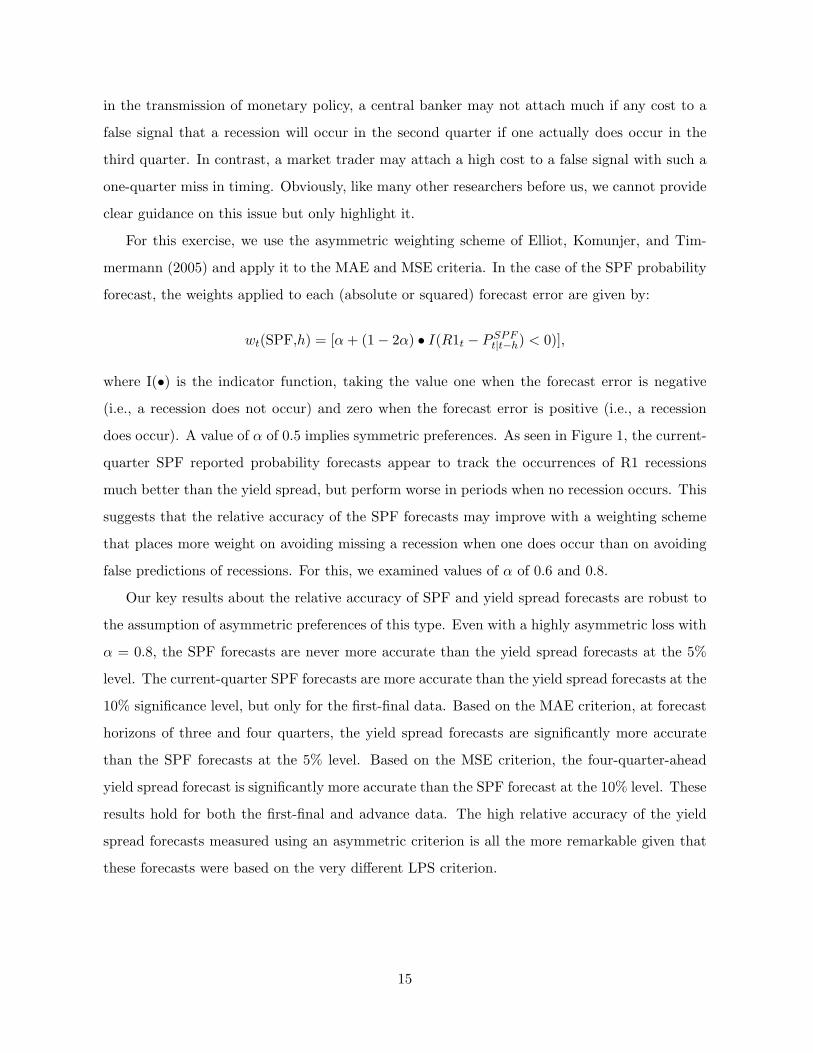
For this exercise, we use the asymmetric weighting scheme of Elliot, Komunjer, and Tim-
mermann (2005) and apply it to the MAE and MSE criteria. In the case of the SPF probability
forecast, the weights applied to each (absolute or squared) forecast error are given by:
where I(•) is the indicator function, taking the value one when the forecast error is negative
(i.e., a recession does not occur) and zero when the forecast error is positive (i.e., a recession
does occur). A value of α of 0.5 implies symmetric preferences. As seen in Figure 1, the current-
quarter SPF reported probability forecasts appear to track the occurrences of R1 recessions
much better than the yield spread, but perform worse in periods when no recession occurs. This
suggests that the relative accuracy of the SPF forecasts may improve with a weighting scheme
that places more weight on avoiding missing a recession when one does occur than on avoiding
false predictions of recessions. For this, we examined values of α of 0.6 and 0.8.
Our key results about the relative accuracy of SPF and yield spread forecasts are robust to
the assumption of asymmetric preferences of this type. Even with a highly asymmetric loss with
α = 0.8, the SPF forecasts are never more accurate than the yield spread forecasts at the 5%
level. The current-quarter SPF forecasts are more accurate than the yield spread forecasts at the
10% significance level, but only for the first-final data. Based on the MAE criterion, at forecast
horizons of three and four quarters, the yield spread forecasts are significantly more accurate
than the SPF forecasts at the 5% level. Based on the MSE criterion, the four-quarter-ahead
yield spread forecast is significantly more accurate than the SPF forecast at the 10% level. These
results hold for both the first-final and advance data. The high relative accuracy of the yield
spread forecasts measured using an asymmetric criterion is all the more remarkable given that
these forecasts were based on the very different LPS criterion.
15
5 Have Forecasters Learned to Use Yield Curve Information?
We regard the result that the simple yield curve model outperforms professional forecasters
at forecasting recessions as very puzzling. One possible explanation is that forecasters were
unaware of the predictive power of the yield curve for much of our sample, which starts at
the end of the 1960s. We therefore reexamine our results using forecast errors from 1988 on.
As mentioned above, the early papers trumpeting the predictive power of the yield curve were
already published or widely circulated around the start of this subsample. Therefore, economists
by then should have incorporated this information in their forecasts and the puzzling predictive
power of the yield curve model over that of the SPF should have vanished. The results for the
post-1987 sample are reported in the right-hand-most columns of Tables 1 and 2.
In the post-1987 sample, the yield spread still contains predictive information that appears
not to have been taken into account by the SPF participants at horizons of three and four
quarters. Based on the first-final data, the yield spread forecasts are significantly more accurate
than the SPF forecasts in half of the cases of forecast horizons of three quarters and longer. The
results are even stronger using the advance data. The upward bias in forecasts is larger for both
the SPF and the yield curve forecasts for this subsample, reflecting the reduced frequency of
recessions during this period relative to earlier decades. For horizons of three and four quarters,
the smaller mean error of the yield curve model explains much of its better performance over
this sample, but it also performs better in quarters when a recession did occur. The rationality
tests of SPF GDP forecasts over this subsample, reported in Table 3, provide some evidence
that economists also failed to heed the information in the yield curve in making GDP forecasts.
Specifically, the four-quarter-ahead forecasts fail the rationality test when the yield spread is
included in the regression.
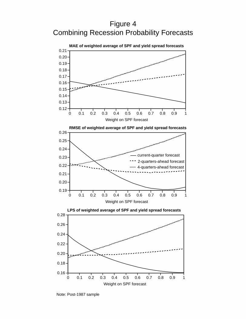
The relative value of the yield spread versus the SPF for forecasting recessions in the post-
1987 sample can also be illustrated by examining the accuracy of the weighted average probability
forecast
PAV Gt|t−h = λPSPF
t|t−h + (1− λ)P Y St|t−h,
where λ is the weight on the real-time SPF reported probability and (1 − λ) is the weight on
the real-time probability forecast based on the yield spread. Figure 4 shows the accuracy, for
the three different measures, of these weighted average forecasts at horizons of h = 0, 2, 4. For
16
forecasting the current quarter (the solid lines), the optimal weight λ is close to one, so the
yield spread adds nothing, but for a four-quarter horizon (the dotted lines), the optimal weight
is zero, so the SPF adds nothing. At a forecast horizon of four quarters, it is clear that one of
the failings of the SPF reported probabilities is the sustained 20% or so chance of a recession
during the long expansions of the past two decades.
6 Conclusion
As witnessed by the public attention to recent pronouncements of probabilities of recession,
there is a great deal of interest in predicting recessions. Nonetheless, economists have a very
spotty track record of predicting downturns. One possible explanation is that recessions are
simply unpredictable. But, this view is contradicted by evidence that the yield curve provides
useful information for forecasting future periods of expansion and contraction. In this paper,
we show that the yield curve has significant real-time predictive power for distinguishing be-
tween expansions and contractions several quarters out relative to the predictions of professional
macroeconomic forecasters. Indeed, we find that a simple model for predicting recessions that
uses only real-time yield curve information would have produced better forecasts of recessions
at horizons beyond two quarters than the professional forecasters provided. This conclusion
remains true during the past 20 years, despite the fact that the yield curve model’s usefulness
has been widely known since the late 1980s.
There are a number of potential reconciliations for this puzzle. One possibility is that
forecasters may have down-weighted the yield curve information because they systematically
underestimated the macroeconomic repercussions of changes in the stance of monetary policy as
proxied for by shifts in the slope of the yield curve. Indeed, the relationship between output and
interest rates is estimated very imprecisely and is subject to econometric difficulties that may
bias estimates of the interest rate sensitivity of output downward. Nonetheless, the longevity of
this puzzle makes one question why forecasters have not caught on to this mistake. Finally, it
is interesting to note that many times during the past 20 years forecasters have acknowledged
the formidable past performance of the yield curve in predicting expansions and recessions but
argued that this past performance did not apply in the current situation. That is, signals from
the yield curve have often been dismissed because of supposed changes in the economy or special
factors influencing interest rates. This paper, however, shows that the puzzling power of the yield
17
curve to predict recessions relative to that of professional forecasters appears to have endured,
despite the wide dissemination of knowledge about the yield curve’s predictive power.
18
References
Ang, A., Piazzesi, M., and Wei, M. (2006), “What Does the Yield Curve Tell Us AboutGrowth?,” Journal of Econometrics, 131, 359-403.
Aruoba, S., Diebold, F.X., and Scotti, C., (in press), “Real-Time Measurement of BusinessConditions,” Journal of Business and Economics Statistics.
Campbell, S. D. (2007), “Macroeconomic Volatility, Predictability and Uncertainty in the GreatModeration: Evidence From the Survey of Professional Forecasters,” Journal of Businessand Economics Statistics, 25, 191-200.
Chauvet, M., and Potter, S. (2005), “Predicting a Recession: Evidence From the Yield Curvein the Presence of Structural Breaks,” Journal of Forecasting, 24, 77-103.
Christensen, J.H., Diebold, F.X., Rudebusch, G.D., and Strasser, G.H. (2008), “MultivariateComparisons of Predictive Accuracy,” Federal Reserve Bank of San Francisco, unpublishedmanuscript.
Corradi, V., and Swanson, N.R. (2006), “Predictive Density Evaluation,” in Handbook of Eco-nomic Forecasting, eds. C.W.J. Granger, G. Elliot, and A. Timmerman, Amsterdam:Elesvier, pp. 197-284.
Corradi, V., Fernandez, A., and Swanson, N.R. (in press), “Information in the Revision Processof Real-Time Datasets,” Journal of Business and Economics Statistics.
Croushore, D. (1993), “Introducing: The Survey of Professional Forecasters,” Federal ReserveBank of Philadelphia Business Review, November/December, 3–13.
Diebold, F.X., and Mariano, R.S. (1995), “Comparing Forecast Accuracy,” Journal of Businessand Economics Statistics, 13, 253-265.
Diebold, F.X., and Rudebusch, G.D. (1989), “Scoring the Leading Indicators,” Journal ofBusiness, 62, 369-391.
Diebold, F.X., and Rudebusch, G.D. (1991a), “Forecasting Output with the Composite LeadingIndex: A Real-Time Analysis,” Journal of the American Statistical Association, 86, 603-610.
Diebold, F.X., and Rudebusch, G.D. (1991b), “Turning Point Prediction With the CompositeLeading Index: An Ex Ante Analysis,” in Leading Economic Indicators: New Approachesand Forecasting Records, eds. Lahiri and Moore, Cambridge: Cambridge University Press,231-256.
Diebold, F.X., and Rudebusch, G.D. (1992), “Have Postwar Economic Fluctuations Been Sta-bilized?,” American Economic Review, 82, 993-1005.
Diebold, F.X., and Rudebusch, G.D. (1996), “Measuring Business Cycles: A Modern Perspec-tive,” Review of Economics and Statistics, 78, 67-77.
Dotsey, M. (1998), “The Predictive Content of the Interest Rate Term Spread for FutureEconomic Growth,” Federal Reserve Bank of Richmond Economic Quarterly, 84, 31-51.
19
Elliot, G., Komunjer, I., and Timmermann, A. (2005), “Estimation and Testing of ForecastRationality Under Flexible Loss,” Review of Economic Studies, 72, 1107-1125.
Estrella, A. (2005), “Why Does the Yield Curve Predict Output and Inflation?” The EconomicJournal, 115, 722-744.
Estrella, A., and Hardouvelis, G.A. (1991), “The Term Structure as a Predictor of Real Eco-nomic Activity,” The Journal of Finance, 46, 555-576.
Estrella, A., and Mishkin, F.S. (1998), “Predicting U.S. Recessions: Financial Variables asLeading Indicators,” The Review of Economics and Statistics, 80, 45-61.
Estrella, A., Rodrigues, A.P., and Schich, S. (2003), “How Stable Is the Predictive Power ofthe Yield Curve? Evidence from Germany and the United States,” Review of Economicsand Statistics, 85, 629-644.
Estrella, A., and Trubin, M.R. (2006), “The Yield Curve as a Leading Indicator: Some PracticalIssues,” Federal Reserve Bank of New York, Current Issues in Economics and Finance 12.
Fernald, J., and Trehan, B. (2006), “Is a Recession Imminent?,” Federal Reserve Bank of SanFrancisco Economic Letter, 2006-32.
Galbraith, J., and van Norden, S. (2007), “The Resolution and Calibration of ProbabilisticEconometric Forecasts,” unpublished manuscript.
Havey, C.R. (1989), “Forecasts of Economic Growth From the Bond and Stock Markets,”Financial Analysts Journal September/October, 38-45.
Kiefer, N. M., and Vogelsang, T.V. (2002) “Heteroskedasticity-Autocorrelation Robust Stan-dard Errors Using The Bartlett Kernel Without Truncation,” Econometrica, 70(5), Septem-ber, 2093-2095.
Kiefer, N.M., Vogelsang, T.J., and Bunzel, H. (2000), “Simple Robust Testing of RegressionHypotheses,” Econometrica 68(3), May, 695-714.
Lahiri, K., and Wang, G.J. (2006), “Subjective Probability: Forecasts for Recessions,” BusinessEconomics 41, 26-36.
National Bureau of Economic Research (2003), “The NBER’s Business-Cycle Dating Proce-dure,” unpublished manuscript.
Stock, J. H., and Watson, M.W. (1989), “New Indices of Coincident and Leading Indicators,”in NBER Macroeconomic Annual 4, eds. O. Blanchard and S. Fischer, Cambridge, MA:The MIT Press, 351-394.
Tulip, P. (2005), “Has Output Become More Predictable? Changes in Greenbook ForecastAccuracy,” Finance and Economics Discussion Series, 2005-31, Federal Reserve Board.
Wright, J. (2006), “The Yield Curve and Predicting Recessions,” Finance and Economics Dis-cussion Series, 2006-07, Federal Reserve Board.
20
Zarnowitz, V., and Braun, P.A. (1993), “Twenty-two Years of the NBER-ASA Quarterly Eco-nomic Outlook Surveys: Aspects and Comparisons of Forecasting Performance,” in Busi-ness Cycles, Indicators, and Forecasting, eds. J.H. Stock and M.W. Watson, Chicago:University of Chicago Press.
21
Table 1
Evaluation of Real-time Probability Forecasts: First-Final Data
Probability Full sample Post-1987 sampleforecast MAE RMSE LPS MAE RMSE LPS
Note: The most accurate entries at each horizon are shown in boldface type. The dagger denotesyield curve forecasts that are significantly more accurate than the SPF reported forecast at the5% level.
22
Table 2
Evaluation of Real-time Probability Forecasts: Advance Data
Probability Full sample Post-1987 sampleforecast MAE RMSE LPS MAE RMSE LPS
Note: The most accurate entries at each horizon are shown in boldface type. The dagger denotesyield curve forecasts that are significantly more accurate than the SPF reported forecast at the5% level.
Note: A dagger denotes coefficients that are significantly different from zero at the 5% level.Each column reports the results from a regression of the SPF real-time real GDP forecast error(assessed using first-final data) on the specified explanetory variables. The row labeled “F-test”reports the p-value associated with the test that all coefficients are jointly zero.
24
SPF reported recession probability forecastsSPF implied recession probability forecasts using fitted normal GDP forecast error distributions
Legend:
Note: Shaded bars denote R1 recession quarters.
68 72 76 80 84 88 92 96 00 040
0.10.20.30.40.50.60.70.80.9
1Current-quarter forecasts
68 72 76 80 84 88 92 96 00 040
0.10.20.30.40.50.60.70.80.9
1One-quarter-ahead forecasts
68 72 76 80 84 88 92 96 00 040
0.10.20.30.40.50.60.70.80.9
1Two-quarter-ahead forecasts
68 72 76 80 84 88 92 96 00 040
0.10.20.30.40.50.60.70.80.9
1Three-quarter-ahead forecasts
68 72 76 80 84 88 92 96 00 040
0.10.20.30.40.50.60.70.80.9
1Four-quarter-ahead forecasts
Figure 1SPF R1 Recession Probabilities
68 72 76 80 84 88 92 96 00 04-1.2
-1.0
-0.8
-0.6
-0.4
-0.2
0Forecasting current quarterForecasting two quarters aheadForecasting four quarters ahead
68 72 76 80 84 88 92 96 00 04-1.2
-1.0
-0.8
-0.6
-0.4
-0.2
0.0
0.2
0.4Forecasting current quarterForecasting two quarters aheadForecasting four quarters ahead
Sequence of intercept estimates
Sequence of slope coefficient estimates
Figure 2Coefficient Estimates from Real-time
Probit Regressions
Note: Probit regressions have R1 recession probability as the left-hand-side variable. Expanding sample real-time estimation begins with 10 years of data starting in 1955:Q1. Forecasts for each quarter use vintage data estimated through a year prior.
68 72 76 80 84 88 92 96 00 040
0.2
0.4
0.6
0.8
1
68 72 76 80 84 88 92 96 00 040
0.2
0.4
0.6
0.8
1
68 72 76 80 84 88 92 96 00 040
0.2
0.4
0.6
0.8
1
68 72 76 80 84 88 92 96 00 040
0.2
0.4
0.6
0.8
1
68 72 76 80 84 88 92 96 00 040
0.2
0.4
0.6
0.8
1
Recession in current quarter Recession one quarter ahead
Recession two quarters ahead Recession three quarters ahead
Recession four quarters ahead
Note: Shaded bars denote R1 recession quarters.
Yield spread R1 recession probability forecasts from real-time probit regressions
Legend:
SPF reported R1 recession probability forecasts
Figure 3SPF and Yield Spread R1 Recession Probabilities
RMSE of weighted average of SPF and yield spread forecasts
0 0.1 0.2 0.3 0.4 0.5 0.6 0.7 0.8 0.9 10.16
0.18
0.20
0.22
0.24
0.26
0.28
Weight on SPF forecast
LPS of weighted average of SPF and yield spread forecasts
Figure 4Combining Recession Probability Forecasts
JBES web appendix for
Forecasting Recessions:
The Puzzle of the Enduring Power of the Yield Curve
Glenn D. Rudebusch∗ John C. Williams†
July 2008
∗Federal Reserve Bank of San Francisco; www.frbsf.org/economists/grudebusch; [email protected].†Federal Reserve Bank of San Francisco; [email protected].
1
1 Defining Recessions
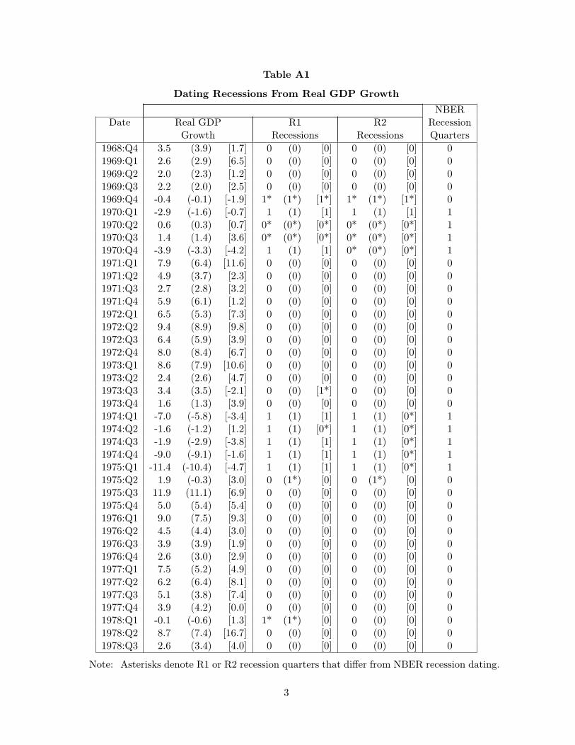
Our chronology of quarterly NBER recessions and expansions is shown in the final column of
Table A1, with a one for a recession quarter and a zero otherwise. This binary variable will be
denoted as RNBERt.
For our analysis, we employ a simple rule that links declines in real GDP to recessions.
Of course, as in any real-time analysis, the issue of which vintage of data to use is important.
The first three columns of Table A1 displays three data series for real GDP growth. The first
series is the so-called “first-final” data which is released about three months after the end of
each quarter. This is our preferred real-time measure of GDP. It incorporates a great deal of
information about expenditures and is a reasonably accurate measure of GDP based on the
methodology in place at the time. The second column, the numbers in parentheses, reports the
latest revised estimates available as of February 2007. These data have been subject to multiple
revisions and, importantly, incorporate significant changes in methodology, making comparison
of real-time forecasts to revised data problematic. The third column, the numbers in square
brackets, reports the “advance” data, which are released about one month after the end of
the quarter. At the time of publication of these data, several important source data are still
unavailable, making these estimates subject to greater measurement error than the first-final
estimates.
A straightforward rule for defining recessions that works quite well is what we dub the
“R1 rule,” which simply defines any single quarter of negative real GDP growth as a recession
quarter. The associated binary variable of recession quarters is denoted as R1t. Columns four
through six in Table A1 report the R1 data for the first-final, current vintage, and advance data,
respectively. A value of one indicates that the growth rate of real GDP was negative in that
quarter, otherwise the value is zero. As shown in the table, the R1 rule applied to first-final data
produces 14 recession quarters that match one of the 21 NBER recession quarters, with only
seven missed calls of recession. The R1 rule also produces five false calls of recession (including
one by a whisker in 1978:Q1). Therefore, there are 12 total quarters of incorrect signals and the
mix of missed calls is reasonably balanced. The R1 rule has advantages in terms of simplicity
and its direct connection to the survey questions in the SPF and we therefore use it for our
analysis for the remainder of the paper.
For comparison, we also report the recession dates that one obtains by applying what we
1
call the “R2 rule,” which defines a recession as occurring if there are two consecutive quarters of
negative real GDP growth. In particular, we say that a quarter is in an R2 recession if real GDP
falls in that quarter and if either (or both) the previous and following quarters post negative
real GDP growth as well. Columns seven through nine in Table A1 report the R2 data for
the first-final, current vintage, and advance data, respectively. This definition of a recession is
often mentioned in the media, but in practice, it performs rather poorly as a proxy for NBER
recession dates. Using any of the three vintages of data, the R2 rule appears too stringent a
criterion to provide a good match to the NBER business-cycle dating methodology. For example,
applying the R2 rule to the first-final data produces only ten recession quarters that match one
of the 21 NBER recession quarters, with 11 quarters of missed recession signals. Perhaps most
problematic, the R2 rule using the first-final data completely misses the 1980 and 2001 NBER
recessions. The R2 rule produces only two false calls of recession quarters relative to the NBER
definition (in 1969 and 1991). Overall then, the R2 rule gives a total of 13 quarters of incorrect