Forecasting Recessions Using the Yield Curve ∗ Marcelle Chauvet and Simon Potter † June 2001 Abstract We compare forecasts of recessions using four different specifica- tions of the probit model: a time invariant conditionally independent version; a business cycle specific conditionally independent model; a time invariant probit with autocorrelated errors; and a business cycle specific probit with autocorrelated errors. The more sophisticated versions of the model take into account some of the potential underlying causes of the documented predic- tive instability of the yield curve. We find strong evidence in favor of the more sophisticated specification, which allows for multiple break- points across business cycles and autocorrelation. We also develop a new approach to the construction of real time forecasting of recession probabilities. Keywords: Recession Forecast, Yield Curve, Structural Breaks, Bayesian, Classical Methods. ∗ The views expressed in this paper are those of the authors and do not necessarily reflect the views of the Federal Reserve Bank of New York or the Federal Reserve System. † Address first author: Department of Economics, University of California, Riverside, CA, 92521. Tel: (909) 787-5037 x1587; email: [email protected]. Address second author: Domestic Research, Federal Reserve Bank of New York, NY, 10045. Tel: (212) 720-6309; email:[email protected]. 1
Transcript
Forecasting Recessions Using the Yield Curve∗
Marcelle Chauvet and Simon Potter †
June 2001
Abstract
We compare forecasts of recessions using four different specifica-tions of the probit model: a time invariant conditionally independentversion; a business cycle specific conditionally independent model; atime invariant probit with autocorrelated errors; and a business cyclespecific probit with autocorrelated errors.The more sophisticated versions of the model take into account
some of the potential underlying causes of the documented predic-tive instability of the yield curve. We find strong evidence in favor ofthe more sophisticated specification, which allows for multiple break-points across business cycles and autocorrelation. We also develop anew approach to the construction of real time forecasting of recessionprobabilities.Keywords: Recession Forecast, Yield Curve, Structural Breaks,
Bayesian, Classical Methods.
∗The views expressed in this paper are those of the authors and do not necessarilyreflect the views of the Federal Reserve Bank of New York or the Federal Reserve System.
†Address first author: Department of Economics, University of California, Riverside,CA, 92521. Tel: (909) 787-5037 x1587; email: [email protected]. Address secondauthor: Domestic Research, Federal Reserve Bank of New York, NY, 10045. Tel: (212)720-6309; email:[email protected].
1
1 IntroductionA large recent literature has shown that asset prices have significant pre-dictive content for future economic activity.1 In particular, recent empiricalwork has found evidence of systematic movements in the yield curve andfuture real output growth or recessions across a number of countries2
In general, the yield curve is upward sloped since long-term rates arehigher than short-term ones. However, the slope of the curve tends to becomeflat or inverted before NBER-dated recessions. One of the possible reasonsis that a tight monetary policy may precede a recession. Further, long-termrates reflect financial markets’ expectation for future short-term rates. Hence,a flat or inverted curve might indicate that the market expects that futurereal interest rates should fall in face of a potential future recession or weakeconomic activity.Although the yield curve is a statistically significant predictor of future
activity, the predictive power of the spread is not stable over time. In par-ticular, most models using the yield curve found it difficult to signal the1990 recession in real time.3 One of the possible reasons for parameter in-stability of models using the yield curve is that its predictive power maydepend on whether the economy is responding to real or monetary shocks(and implicitly on the monetary policy reaction function see Hamilton andKim 2000 for a decomposition of the spread). In addition, there have beenhave been numerous changes in the market for U.S. Treasury debt over thelast two decades. For example, recently the Treasury has been buying backdebt leading to a reduction in the supply of long-term Treasury bonds.Another potential reason is the recent changes in the volatility of the
U.S. economy. In particular, McConnell and Perez (2000), Kim and Nelson(1999), and Chauvet and Potter (20001b) find evidence of a break towardsmore stability in the economy since 1984. Since these factors might affectthe relationship between the yield curve and economic activity, models thatdo not take into account these evolving dynamics may lead to poor real timeforecasts.
1See Stock and Watson (2000) for a comprehensive literature review.2The terms ‘yield curve‘, ‘term structure of interest rates’, or simply ‘term spread’ refer
to the difference in return between between long term and short term government bonds.3The exception is Laurent (1989). Harvey (1989) and Stock andWatson (1989) signaled
the economic slowdown that started in 1989. See Stock and Watson’s (2000) for a moredetailed discussion.
2
In general, linear regression models that use output growth as the de-pendent variable indicate that the forecasting ability of the term spread hasreduced since mid 1980s.4 However, models that focus instead on predictinga binary indicator of recession or expansion are more successful and stableover time than continuous ones.5 This evidence is corroborated in the recentwork by Estrella, Rodrigues, and Schich (2000) (ERS hereafter), who exam-ine the stability of the predictive model using classical tests for an unknownsingle breakpoint. They find evidence of structural break in the continuousmodel of U.S. industrial output in late 1983, but no evidence of instabilityover the full sample using binary models.6
In contrast with the results of ERS, Chauvet and Potter (2001a) find over-whelming evidence of structural instability when the binary probit model isestimated using the Gibbs sampler. The probability of recessions is sub-stantially affected by consideration of a breakpoint as well as its location.Although the model used considered only a single break, there was evi-dence of the presence of multiple breakpoints. One possible resolution ofthese differing results is the presence of autocorrelated errors in the probitmodel. ERS adjust their test statistics for the presence of autocorrelationand heteroscedasticity under the null hypothesis, whereas Chauvet and Pot-ter (2001a) use Bayesian tests that are not amenable to such non-parametricadjustment techniques.7 The potential effects on forecasting of not explicitlymodeling correlation in the errors is large, and examining its importance isone of the main goals of this paper.We extend the probit specification of Estrella and Miskin (1998) (EM
hereafter) to account for these two forms of potential misspecifications: time-varying parameters due to existence of multiple breakpoints, and the pres-ence of autocorrelated errors. We examine the predictive content of the term
4See, for example, Haubrich and Dombrosky (1996), Dotsey (1998), Friedman andKuttner’s (1998) or Stock and Watson’s (2000) survey.
5See Neftci (1996), Dueker (1997), Estrella and Mishkin (1998), and Estrella, Ro-drigues, and Schich (2000).
6They use real industrial production and the spread between 10 year and 1 year interestinterest rates from 1967:01 to 1998:12.
7For example, if we assume a break in the first month of 1984, the maximized likelihoodof the model with a break is 1000 times that of a model without a break. In the classical testused by ERS this difference is not statistically significant after allowing for autocorrelatederrors under the null hypothesis and the endogenity of the breakpoint. In contrast, theBayesian test compares the average (over the prior distribution) height of the likelihoodbetween the two models and makes no correction for misspecification of either model.
3
structure in forecasting recessions under four different specifications: a timeinvariant conditionally independent version, as in EM, a time-varying con-ditionally independent version that takes into account multiple breakpointsacross business cycles, a time invariant probit model with autocorrelated la-tent variable, and a time-varying probit model with autocorrelated latentvariable.In the standard probit model of EM conditional on the observed yield,
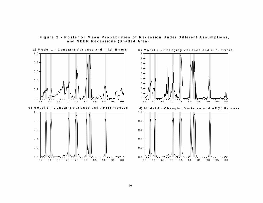
the probabilities of the recession states are independent of each other (thisfollows directly from the assumption of independent errors). Figure 2a showsthe implied probability of a recession state each month from 1955 throughthe end of 2000.8 Notice that until 1995-96 the probability of any particularmonth being a recession state was relatively low in the current expansion.Under the independence assumption, one can easily calculate the probabilityof not observing a recession over the 117 months from April 1991 to Decem-ber 2000. For example, if the probability of a recession had remained fixedat the low value of 0.025, the probability of not observing a recession (i.e.,continuing expansion for 117 months) would be (0.975)117, which is approx-imately 5%. In other words, the probability of a recession occuring wouldbe 95% (i.e., the probability that the first hitting time to a recession is 117months or less). Alternatively, if we use the 60 estimated probabilities sincethe end of 1995 to 2000 from Figure 2a, we obtain a 12.5% probability of norecession through the period of 1996-1997, 5% through the period of 1996-1998, 0.5% through the period of 1996-1999, and an effectively 0 probabilityof no recession through the period of 1996-2000.9 These low probabilitiesof continuing expansion indicate that either the 1990s represent a period ofextraordinary good luck or that the probit model suffers from some severemisspecification.In this paper we estimate and compare probabilities of recession using al-
ternative probit specifications. We use probabilities of continuing expansionand first recession time as described in the previous paragraph for producingforecasts. We believe that these probabilities provide more accurate real time
8The probabilities come from a standard probit model estimated by the Gibbs sampler(maximum likelihood techniques produce virtually identical results), using yield data fromJanuary 1954 to December 1999 and NBER business cycle dates from January 1955 toDecember 2000. Thus, we are assuming that the U.S economy was still expanding inDecember 2000.
9Note that the decrease in the probabilities of no recession around 1997 and 1999 isassociated with the Asian and Russian currency crisis, respectively.
4
predictions of the likelihood of turning points.10 The models are estimatedand analyzed using Bayesian methods. There are two motivations for the useof Bayesian techniques. The first is that maximum likelihood estimation forprobit models with an autoregressive component is impractical for the size ofdataset used.11 In contrast, the Gibbs sampler can be used to simulate thelatent variable of the probit model, which drastically reduces the computa-tional complexity. Second, we are interested in presenting distributions overthe forecast probabilities that contain information on both parameter un-certainty and uncertainty over the most recent value of the latent variable.These can be directly obtained from the output of the Gibbs sampler. Inaddition, it is computationally simple to calculate Bayes factors to comparethe various models using the Savage-Dickey Density ratio within the Gibbssampler.The Bayes factor indicates overwhelming evidence in favor of the more
complicated specifications. Plots of the in-sample predicted recession proba-bilities indicate that specifications with autocorrelated errors provide a muchcleaner classification of the business cycle into expansion and recession peri-ods. We also compare the performance of the alternative models in a real-time forecasting exercise using yield curve data from January 2000 to March2001. While all the models considered indicate that the yield curve is cur-rently signaling weak future economic activity in 2001-2002, we find that thestrength of a recession signal differs substantially across specifications withweaker signals coming from the more complicated specfications.The paper is organized as follows. The next section introduces the probit
model and discusses our various extensions. The third section outlines theGibbs sampler and the construction of the Bayes factors. In the fourthsection the empirical results from the alternative specifications are discussedand some real time forecasting results presented. The fifth section concludes.
2 Extending the Probit ModelThe probit model assumes an underlying latent variable Y ∗t for which thereexists a dichotomous realization of an indicator Yt denoting the occurrence or
10These probabilities consider uncertainty on both the parameters and the most recentvalues of the latent variable.11The difficulty comes from the fact that it is necessary to evaluate multiple integration
over the unobserved lagged variable.
5
non-occurrence of an event. Here we assume that the variable Y ∗t representsthe state of the economy and we use as its indicator the recession datingprovided by the NBER. Yt can take on two values, 0 if the observation is anexpansion or 1 if it is a recession:
Yt =
½0 if Y ∗t < 01 if Y ∗t ≥ 0 . (1)
In addition, it is useful to have a notation for the specific dates of the businesscycles. We assume that a business cycle starts the month after a NBERtrough and continues up to the month of the next NBER trough. We denotethe business cycle dates n by tn−1+1, . . . tn. Further, we indicate the dates ofthe expansion and recession phases of business cycle n by the sets En and Rn,respectively. Hence, the dates of business cycle expansions and recessions aregiven by E = ∪En and R = ∪Rn, respectively.The unobservable variable Y ∗t is related to the yield curve according to
following regression:
Y ∗t+K = β0 + β1St + εt, (2)
where St is the spread between the 10-year and 3-month Treasury Bill rates,K is the forecast horizon of the latent variable in months, and βi ( i = 0, 1)are the regression coefficients. The error term εt is assumed to be indepen-dently distributed over time with a standard normal distribution. Noticethat multiplying Y ∗t+K by any positive constant does not change the indica-tor variable Yt+K . This implies that the coefficients βi can be estimated onlyup to a positive multiple. Thus, the standard probit model assumes that thevariance of the errors is equal to one in order to fix the scale of Y ∗t+K .From equations (1) and (2) we obtain:
P (Y ∗t+K ≥ 0|St, β) = Φ[β0 + β1St], (3)
where Φ is the cumulative distribution function of the standard normal dis-tribution, and P (Y ∗t+K ≥ 0|St, β) is the conditional probability of a recessionat the forecast horizon K. Note that this is not necessarily the probabilityof most interest in forecasting.
6
As an alternative way of constructing probabilities considers the firsthitting time to a recession given by:
HR(t) = {H : Y ∗t+H > 0, Y∗
t+H−1 < 0, . . . , Y∗
t+1 < 0},
with the associated probability:
πR(k, t) = P [HR(t) = k] = P [Y∗
t+k > 0|Y ∗t+k−1 < 0, . . . , Y∗
t+1 < 0](1− πR(k − 1, t)).
Conditional on a sequence of values for Skt−K = {St−K+1, St−K+2, . . . , St−K+k}
we can evaluate these expressions by:
πR(k, t) = Φ[β0 + β1St−K+k]k−1Ys=1
{1−Φ[β0 + β1St−K+s]} . (4)
Notice that this expression reflects a conditionally constant probability ofrecession, and it is directly related to the likelihood function of the observeddata:
`(Y T |ST−K,β) =Yt∈R
Φ[β0 + β1St−K ]Yt∈E
{1−Φ[β0 + β1St−K ]} , (5)
where β = [β0, β1]0.
In addition, the ordering ofQk−1
s=1 {1− Φ[β0 + β1St]} makes no differenceto the hitting probability or to the value of the likelihood function. Thisis a direct consequence of the assumption of conditional independence andconstant relationship between the yield spread and the probability of reces-sions. In particular, if we consider two expansions where the values of theterm spread are given by permutations on the set
{St−K+1, St−K+2, . . . , St−K+k−1},
and fix the most recent value at St−K+k, they will have exactly the sameprobabilities of the expansion ending at time T + k.We extend this framework in two main ways. First, we allow the variance
of the innovation to change with the business cycle, which accounts for po-tential structural breaks in the relationship between the yield curve and theeconomy. Second, we add an autoregressive component to the model.
7
2.1 Business Cycle Specific Model
We consider a more general specification of the probit model in which thevariance of the innovation may change across the N business cycles:
Y ∗t = β0 + β1St−K + σ(t)εt, (6)
where
σn = σ(t) if tn−1 < t ≤ tn, n = 1, . . .N,
and the initial business cycle is partially observed starting at t = K + 1(t1 = K). Hence, even in the case that the collection of yield spreads is thesame, we can obtain different hitting probabilities across business cycle, sincenow we have:
πR(t, k) = Φn [β0 + β1St−K+k]k−1Ys=1
{1− Φn[β0 + β1St−K+k]} . (7)
where
Φn[β0 + β1St] = Φ[(β0 + β1St)/σn].
There are two interpretations of this model. The first is the literal one thatshocks to the latent variable may change over business cycles. For example,one could imagine that a long business cycle has a smaller innovation variancethan a short one. The alternative interpretation arises from the fact that thescale of the innovation and the coefficient parameters βi can not be separatelyidentified. Thus, we can think of this as a time-varying parameter model, inwhich the innovation variance is normalized to 1 across all business cycles,but each cycle has a unique intercept βn0 = β0/σn and slope βn1 = β1/σn.The likelihood function for the business-cycle specific variance is now:
`(Y T |ST−K,β, {σn}) =NY
n=1
µ Qt∈Rn
Φn[β0 + β1St−K ]Qt∈En
{[1−Φn[β0 + β1St−K ]}¶, (8)
and now is grouped into particular expansions and contractions.
8
2.2 Dependence in the Latent Variable
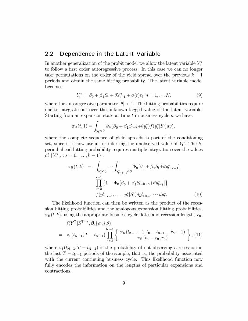
In another generalization of the probit model we allow the latent variable Y ∗tto follow a first order autoregressive process. In this case we can no longertake permutations on the order of the yield spread over the previous k − 1periods and obtain the same hitting probability. The latent variable modelbecomes:
Y ∗t = β0 + β1St + θY∗
t−1 + σ(t)εt, n = 1, . . . N. (9)
where the autoregressive parameter |θ| < 1. The hitting probabilities requireone to integrate out over the unknown lagged value of the latent variable.Starting from an expansion state at time t in business cycle n we have:
πR(t, 1) =
Zy∗t <0
Φn(β0 + β1St−k+θy∗t )f(y
∗t |St)dy∗t ,
where the complete sequence of yield spreads is part of the conditioningset, since it is now useful for inferring the unobserved value of Y ∗t . The k-period ahead hitting probability requires multiple integration over the valuesof {Y ∗t+s : s = 0, . . . , k − 1} :
The likelihood function can then be written as the product of the reces-sion hitting probabilities and the analogous expansion hitting probabilities,πE(t, k), using the appropriate business cycle dates and recession lengths rn:
`(Y T |ST−k,β,{σn},θ)
= πI(tN−1, T − tN−1)N−1Yn=2
½πR(tn−1 + 1, tn − tn−1 − rn + 1)
πE(tn − rn, rn)
¾, (11)
where πI(tN−1, T − tN−1) is the probability of not observing a recession inthe last T − tN−1 periods of the sample, that is, the probability associatedwith the current continuing business cycle. This likelihood function nowfully encodes the information on the lengths of particular expansions andcontractions.
9
3 Estimation and Forecasting TechniquesThe model with an autoregressive process for the latent variable is difficultto estimate using maximum likelihood, since multiple integration over theunobserved lagged variable is required. Thus, we use the Gibbs sampler toevaluate the likelihood function.12 Further, since we are interested in out-of-sample estimates of the hitting probabilities of recessions, we focus on theproperties of the joint posterior distribution of the model parameters andmost recent value of the latent variable.
3.1 Obtaining Draws of the Latent Variable
The Gibbs sampler proceeds by generating draws of the latent Y ∗t conditionalon (β0,β1, {σn}, θ) and the observed term spread. To simplify notation, letX 0
tβ = β0 + β1St−k. If θ = 0, then the sampler would have the followingsimple form:
1. Draw εt from the truncated normal on (−∞,−X 0tβ/σn) if t is an ex-
pansion period of business cycle n .
2. Draw εt from the truncated normal on [−X 0tβ/σn,∞) if t is a recession
period of business cycle n.
The presence of the lagged value of the latent variable in the conditionalmean complicates the sampler. Consider first generating the last value inthe observed sample, Y ∗T . If we could condition on a value for Y
∗T−1, then we
could use the steps above by redefining X 0Tβ = β0 + β1ST−K + θY
∗T−1. This
would generate a draw of the last period value of the latent variable.Now with this “new” value of Y ∗T and the “old” value of Y
∗T−2, we can use
the a priori joint normality of the underlying latent variable model to form aconditional normal distribution for Y ∗T−1. The exact form of this distributiondepends on an assumption about the initial value Y ∗K. We simplify the anal-ysis by assuming that Y ∗K = β0+ β1S0 = 0. Then, as shown in the appendix,
12See Geweke 1999 and Chib 2001 for excellent introductions to modern Bayesian com-putational techniques and references to earlier work on probit models that we implicitlydraw on.
10
we have a priori the conditional normal distribution with mean:
eXT−1 + θ
"V (eYT−1)
V (eYT−2)
#"V (eYT ) θ2V (eYT−2)
θ2V (eYT−2) V (eYT−2)
#−1 "Y ∗T − eXT
Y ∗T−2 − eXT−2
#,
and variance:
V (eYT−1)− θ2
"V (eYT−1)
V (eYT−2)
#"V (eYT ) θ2V (eYT−2)
θ2V (eYT−2) V (eYT−2)
#−1 "V (eYT−1)
V (eYT−2)
#0,
where
V (eYt) =t−K−1X
s=0
θ2sσ2(t− s)
and
eXt =t−K−1X
s=0
θsX 0t−sβ.
Hence, we draw from the appropriate truncated normal as above to obtaina new draw of Y ∗T−1. This process continues until we arrive at the initialobservation period. The value of Y ∗K+1 is drawn in a similar manner to Y
∗T ,
by conditioning on the new draw of Y ∗K+2. However, this value has a differentform, since its mean is given by:
X 0K+1β +
θσ2(1)
σ2(1) + θ2σ2(2)
³Y ∗K+2 − eX 0
K+2
´,
and variance by:
σ2(1)− θ2σ4(1)
σ2(1) + θ2σ2(2).
11
3.2 Obtaining Draws of Probit Model Parameters
Given this sequence of draws for {Y ∗t }, we then need to obtain draws ofthe parameters (β, {σn}, θ). For simplicity, we use prior distributions fromparametric families that generate simple conditional distributions for theposterior.13 We assume that the parameters of the conditional mean β area priori bivariate normal with mean vector µ(β) and variance matrix V (β).In addition, the autoregressive parameter θ is assumed to have an a prioritruncated normal on (−1, 1) with mean µ(θ) and variance V (θ) independentof β. Finally the N − 1 variance parameters are assumed to be a prioriindependent with identical inverted gamma distributions.For a draw of β, define the time series Zt = (Y
∗t −θY ∗t−1). Then, conditional
on ({Y ∗t }, {σn}, θ), the parameters β are obtained from a normal distributionwith variance matrix:
V (β) =
"V (β)−1 +
TXt=K+1
XtX0t/σ
2(t)
#−1
,
and mean vector:
µ(β) = V (β)
"V (β)−1µ(β) +
TXt=K+1
XtZt/σ2(t)
#.
For a draw of θ, define the time series Wt = (Y∗
t −X 0tβ). Then, conditional
on ({Y ∗t }, {σn},β) a potential draw for θ is from a normal distribution withvariance:
V (θ) =
"V (θ)−1 +
TXt=K+1
Y ∗2t−1/σ
2(t)
#−1
,
and mean:
µ(θ) = V (θ)
"V (θ)−1µ(θ) +
TXt=K+1
Y ∗t−1Wt/σ2(t)
#.
13The sampler will require draws from normal and gamma distributions. Random drawsfrom both types of distributions are available in widely used packages such as Gauss andMatlab.
12
If this draw satisfies the stationary condition, it is accepted. If not, it isrejected and new draws are made until one is obtained that satisfies thestationarity condition.For draws of {σn}, we assume that the prior distributions are independent
inverted gammas with identical degrees of freedom ν and scale νs2. Hence,the prior mean is νs2/(ν − 2). The prior parameters are then updated forbusiness cycle n ≥ 2 by:
νn = ν + tn − tn−1
νs2n = νs2 +
tnXt=tn−1+1
(Y ∗t −X 0tβ − θY ∗t−1)
2.
3.3 Bayes Factors
We are interested in the recession probabilities obtained from four differentmodels:
1. Model 1: a probit specification with constant variance and seriallyuncorrelated latent variable;
2. Model 2: a probit specification with business cycle specific varianceand serially uncorrelated latent variable;
3. Model 3: a probit specification with constant variance and autoregres-sive latent process;
4. Model 4: a probit specification with business cycle specific varianceand autoregressive latent process.
We use Bayes factors to assess the value-added of the business cycle spe-cific variances and autoregressive structure specifications. That is, we com-pare the marginal likelihoods of the various models, which correspond to theaverage height of the likelihood of the observed data (i.e., the NBER businesscycle dates) with respect to the prior distribution. In some situations, theBayes factor corresponds to the likelihood ratio statistic. For example, thelikelihood ratio and Bayes factor are equal for the case of testing the probitmodel with autoregressive errors and time invariant variance, with θ = 0.8,against the conditionally independent time invariant probit model with allother parameters known.
13
More generally, the Bayes factor differs from the likelihood ratio by theway it integrates out nuisance parameters and averages over possible param-eter values for the alternative model. In order for these operations to makesense, it is necessary that the prior distributions are proper, that is, thatthey integrate to 1. For example, if we place an improper prior distributionon θ, its average height over the line is not well-defined. Further, even if wearbitrarily fixed a height for the prior distribution by construction, it wouldplace zero weight on values of θ where the likelihood was higher than in therestricted model.The major disadvantage of marginal likelihoods is their dependence on
the prior distribution and the difficulty in their calculation. As explainedabove, diffuse prior distributions are not appropriate when calculating Bayesfactors. However, we have prior distributions that are sufficiently uninfor-mative so that the sample information will dominate. In our case, we havethe general restriction that θ ∈ (−1, 1). In addition, for the business cyclespecific variances model we choose a prior with a small number of degrees offreedom and with a mean equal to 1.With respect to their calculation, the Bayes factor can be greatly sim-
plified by using the Savage-Dickey Density ratio. If two models are nested,then there exists at least one point in the parameter space of the unrestrictedmodel where its likelihood is equivalent to the restricted model. For exam-ple, if we evaluate our most general model at θ = 0, then its likelihood isequivalent to the business cycle specific probit. In the nested case, the Bayesfactor can be found by the ratio of posterior density at θ = 0 to the priordensity at θ = 0, under some mild regularity conditions. Continuing withthe example the Bayes factor would be:
BF2 vs 4 =p(θ = 0|Data)p(θ = 0)
.
Notice that with Gibbs sampling we do not have direct access to theunconditional posterior densities. Instead, we can calculate them at eachiteration of the sampler as:
we can average these values across draws of the sampler to obtain an estimate.The Bayes factor (BF) is assessed using the recommendations of Jeffrey’s
(1961, Appendix B), which states the weight of evidence against the nullgiven by the following range of values:
• lnBF > 0 evidence supports null;• −1.15 < lnBF < 0 very slight evidence against null;
• −2.3 < lnBF < −1.15 slight evidence against the null;• −4.6 < lnBF < −2.3 strong to very strong evidence against the null;• lnBF < −4.6 decisive evidence against null.
3.4 Real Time Forecasts
The main objective of the analysis of the relationship between the yield curveand business cycle turning points is to provide better real time predictions ofturning points. In the original probit model of EM, forecasts were constructedby using the maximum likelihood estimates and recent observations on theyield curve. For example:
P (Y ∗T +K ≥ 0|ST , bβ) = Φ[bβ0 + bβ1ST ].
Note that since it is unlikely that the predicted probability is exactly equalto 0 or 1 some judgement is required on how to interpret the predictions.We have emphasized a different type of prediction in Section 2, namely theprobability of an expansion continuing for k more months. For the originalprobit specification of EM, this forecast is obtained from:
kYs=1
n1−Φ[bβ0 +
bβ1ST +k−s]o,
where this forecast converges to 0 as k increases by construction.The first difference in prediction using the Gibbs sampler approach is
that instead of evaluating the cumulative distribution function using themaximum likelihood estimator, one evaluates it at each draw of the Gibbs
15
sampler. The collection of forecasts can then be averaged to produce anestimated posterior mean probability of recession:
bP (Y ∗T+K ≥ 0|ST , ST−K ,ψ, YT ) =
1
I
IXi=1
Φ[β{i}0 + β
{i}1 ST ],
where ψ signifies the hyperparameters of the prior distributions and the as-sumption on the initial conditions of the latent variable and the yield curve.Alternatively, the posterior predictive distribution can be analyzed directlyand used to present probability intervals on the probability of recession.Analogously, one can form the cumulative product of the individual prob-abilities at each iteration of the Gibbs sampler and examine its posteriorproperties.The second difference arises from the more complicated model with an au-
toregressive component. In this case, as noted above, one needs to integrateout over the unknown lagged value of the latent variable to form predictions.This requires a numerical integration step at each iteration of the Gibbs sam-pler. The Gibbs sampler produces a draw of Y ∗T , θ, and σN . These valuescan be used to simulate J time series realizations of {Y ∗T +s; s = 1, . . . k} usingthe observed yield values from T −K + 1 to T − 1. The average over theseJ draws is formed as:bP (Y ∗T+K ≥ 0|ST , S
T−K,ψ, Y∗{i}
T , ξ{i}) =
1
J
JXj=1
Φh(β{i}0 + β
{i}1 ST + θ
{i}Y ∗{j}T +k−1)/σ{i}N
i,
where ξ{i} denotes the set of parameter draws at the ith iteration of the Gibbssampler. Averaging this estimated probability over the I draws from theGibbs sampler produces an estimate of the posterior mean of the probabilityof recession and the collection of draws provides an estimate of the posteriordistribution.
4 Results
4.1 Priors
We assume that the prior variance of β is the identity matrix. For the priormean we use the maximum likelihood estimate from model 1, which assumes
16
unit variance and no autoregressive component, as in EM. Given the size ofthe sample there is little influence from the prior. However, we decided togive to EM’s standard probit model the advantage of a prior centered at itsMLE. For the autoregressive parameter θ the prior is taken to be a truncatedstandard normal on (−1, 1). With respect to the prior for the business cyclespecific variances, we center it at 1, with diffuse degrees of freedom equal to3.
4.2 Empirical Results
The data on the yield curve cover the period from January 1954 to March2001.14 We set the forecast horizon K to 12 and assume that no recessionwill be called in the last three months of 2000.15 Thus, our business cycledata run from January 1955 to December 2000. The last 15 observations ofthe yield spread are used to form real time forecasts of the probability ofrecession state for each month from January 2001 to March 2002, and theprobability of an expansion continuing through March 2002.We use 40, 000 iterations to estimate the probit models using the Gibbs
sampler. We start the sampler from the maximum likelihood estimate forthe whole sample from Model 1, but calculate the posterior properties onlyafter 10, 000 draws (thus, 50, 000 draws in total).16
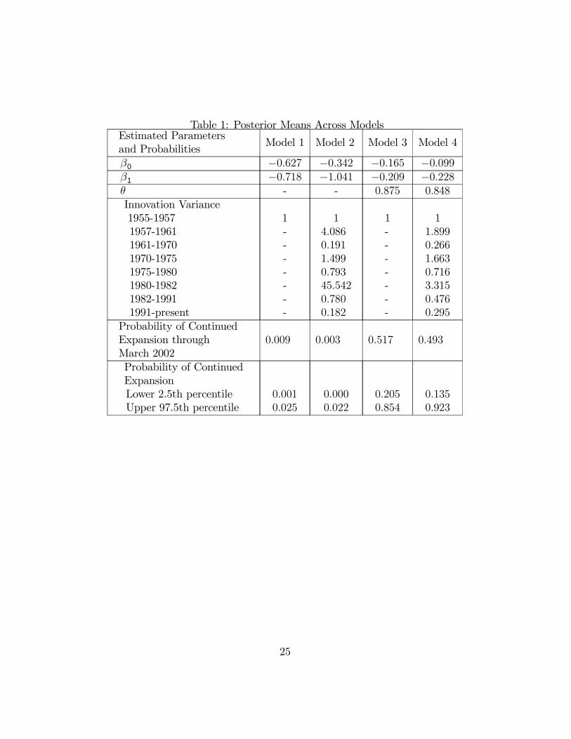
Table 1 summarizes the posterior means of the parameters for the fouralternative specifications and also gives some forecasts of the probability ofrecession in 2001 − 2002. The results from all models corroborate previousfindings, indicating a significant relationship between inversions of the termstructure and the probability of a recession 12 months ahead.The posterior means of the parameters for the different models can not
be directly compared due to the presence of the autoregressive componentand/or business cycle specific variance. However, we can observe that in
14The yield spread is defined as the difference between the 10-year constant maturityTreasury Bond and the 3-month constant maturity Treasury Bill. We take the average ofthe daily rates each month.15Hall (2001) suggests that there the NBER is unlikely to call a recession in the last
quarter of 2000. Robert Hall is one the members of the NBER Business Cycle DatingCommittee.16The computation time for the most complicated model is around 4 hours, including
the construction of the out-of-sample forecasts with the use of 1000 simulated draws foreach Gibbs draw.
17
all cases the posterior mean of the intercept and slope coefficients are neg-ative as expected. Further, the autoregressive parameters in Models 3 and4 are relatively large and positive, implying highly persistent movements inthe underlying latent variable. These results affect the recession forecastssubstantially, as discussed below.Table 1 shows the different values obtained for the variance across the
seven business cycles in the sample for Models 2 and 4, which allow thevariance to change over the business cycle. Except for a scale factor, theestimated variances from these models capture the same features across dif-ferent business cycles in the sample. In particular, the highest estimatedvariance occurs during the short 1980-81 business cycle. This corresponds tothe period in which the Federal Reserve changed its operating procedures.The level and volatility of interest rates and consequently, of the yield curve,increased substantially during the 1979-82 period. On the other hand, thevariances with lowest values are associated with the long expansions of the1960s, 1980s and 1990s.The negative of the posterior means for the latent variable (Y ∗t ) are plot-
ted in Figure 1 together with the yield spread for all four models considered.We can observe that the posterior mean of the latent variable from the sim-plest version of the probit specification (Model 1) does not vary much ascompared to the other models, and essentially tracks the yield curve.This can also be observed in Figure 2, which plots the posterior mean of
the probabilities of recession from January 1955 to March 2002 for all fourspecifications. The probabilities consistently rise before each of the sevenfull recessions in the sample dated by the NBER. However, the probabilitiesof a recession for Model 1 are only above 50% for the 1974-75, the 1980,and the 1981-1982 recessions. In addition, Model 1 gives more false signalsof recessions than the other specifications. Notice that the probabilities ofrecessions from this model rise as much for recessions as for the low-growthphases in the U.S. economy in 1966-67, in 1995, and in 1997, which areassociated, respectively, with slowdowns in Europe, with the Mexican crisis,and with the East Asian crisis. As a result, interpretation of increases inprobabilities as an indication of future recessions is not unambiguous. Thisis also the case for the current slowdown in 2000-2001, as discussed in thenext section.Model 2 allows for the possibility of time-varying parameters or, more
specifically, for variances that may change for each of the recessions in thesample. There are two main differences between the posterior probabilities
18
of recession from Models 1 and 2. First, the posterior probabilities risesubstantially more before each of the NBER-dated recessions in Model 2than in Model 1. Second, Model 2 gives only one false signal of recession —the probabilities forecast the 1966-67 low-growth phase as a recession. Thus,probabilities of recession from Model 2 are easier to interpret as signallingturning points. An interesting feature of this model is that the posteriorlatent variable increases substantially after the 1990-91 recession. Perhapsthe magnitude of the increase in the latent variable is associated with thelong extension of the 1990s expansion.When allowing for an autoregressive process in the probit model, the esti-
mated parameters and posterior probabilities of recessions are quite differentfrom the other specifications. As seen in Figure 2, the posterior probabilitiesfrom Model 3 and 4 are very similar to each other and very different fromModels 1 and 2. In particular, the probabilities of recession from Models 3and 4 consistently increase above 80% before each of the recessions in thesample. Thus, there is much less uncertainty regarding interpretation of theseprobabilities. In addition, the probabilities increase only before recessions,not before slowdowns. That is, the probabilities from these models do notgive any false signals of recession.The Bayes factor allows us to evaluate the sample evidence in favor of
the alternative models. The Bayes factor indicates overwhelming evidence infavor of the specification that includes both business cycle specific varianceand an autoregressive process for the latent variable. This could be expectedgiven the significant improvement in fit produced by the extensions to thebasic probit model, as exhibited in Figure 2. Further, the Bayes factor alwaysfavors the more complicated model in each possible pairwise comparison.First, the natural logarithm of the Bayes factor for constant variance versusbusiness cycle specific variance is −55 (for Model 1 versus 2) and −27 (forModel 3 versus 4) showing decisive evidence for the time varying variance.Second, the Bayes factor for no autoregressive term versus an autoregressiveterm is impossible to distinguish from computer zero. Thus, the sampleevidence decisively supports Model 4.
4.3 Recession Forecasts for 2001-2002
In this section, we illustrate the differences between the various models andalso between the simple recession probabilities and hitting time probabilitiesin a real time forecasting exercise. The exercise uses the 15 months of yield
19
spread data after the end of the estimation sample in December 2000Figure 3 plots the posterior mean of probabilities of recessions for 2001-
2002 for all models. As it can be observed, the probability of recessionsfor this period differ considerably across the alternative specifications. Inparticular, the simplest versions of the probit model that do not correct forserially correlated errors have the highest probabilities of recession states in2001-2002 (Models 1 and 2). Model 2 indicates that the U.S. economy mayexperience a short recession during the second semester of 2001, while Model1 gives more moderate signals of a weak economy. On the other hand, themore sophisticated specifications that allow the latent variable to be seriallycorrelated yield substantially smaller probabilities of a recession in the nearfuture (Models 3 and 4).More specifically, the probabilities of a recession state for particular months
in the second semester of 2001 for Model 1 are around 40%. They reach apeak of 46% in December 2001 and decrease steadily to 27% in March 2002,the last month in the forecast exercise. However, one of the problems withModel 1, in addition to be misspecified, is that it equally signals both re-cessions and slowdowns. Thus, the probabilities may be indicating either apotential recession or simply the continuation of the low-growth phase in theU.S. economy that started in 2000. For Model 2, the probabilities of a re-cession in the second semester of 2001 are substantially higher (around 59%)reaching a peak in December 2001 of 70%. Given the recession probabilityhistory from this model, as observed in Figure 1b, these high values indicatethat the economy may experience a short recession in the second semester of2001. However, the probabilities of recession decline quickly to only 11% inMarch 2002.A more accurate reading on the likelihood of recessions can be obtained
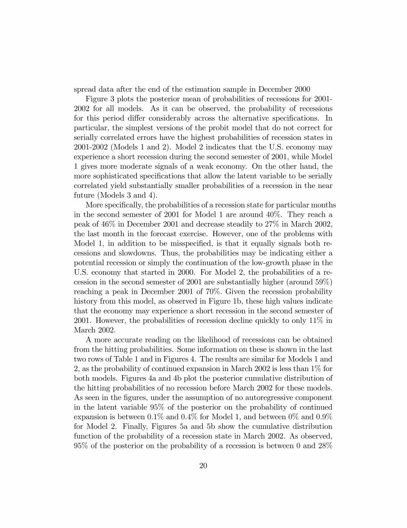
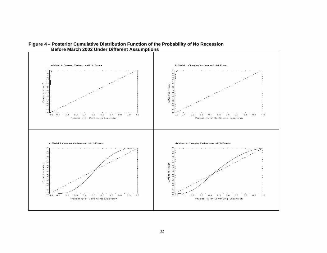
from the hitting probabilities. Some information on these is shown in the lasttwo rows of Table 1 and in Figures 4. The results are similar for Models 1 and2, as the probability of continued expansion in March 2002 is less than 1% forboth models. Figures 4a and 4b plot the posterior cumulative distribution ofthe hitting probabilities of no recession before March 2002 for these models.As seen in the figures, under the assumption of no autoregressive componentin the latent variable 95% of the posterior on the probability of continuedexpansion is between 0.1% and 0.4% for Model 1, and between 0% and 0.9%for Model 2. Finally, Figures 5a and 5b show the cumulative distributionfunction of the probability of a recession state in March 2002. As observed,95% of the posterior on the probability of a recession is between 0 and 28%
20
indicating that the positive steepening of the yield curve in early 2001 signalsstronger economic activity in 2002.On the other hand, when we allow the latent variable to follow an autore-
gressive process, the resulting recession probability forecasts are substantiallysmaller. In particular, the probability of a recession in the second semesterof 2001 is around 18% for both models 3 and 4 (Figures 3c and 3d). Theprobabilities reach a maximum in January 2002 of only 25% for Model 3and 31% for Model 4, and slowly decrease until March 2002. As observed inFigures 2c and 2d, the probabilities from these models increase above 80%before each of the recessions in the sample.However, the evidence from the hitting probabilities show higher uncer-
tainty with respect to a future recession. In particular, the probabilitiesthat a expansion will continue in March 2002 are around 50% for Models 3and 4 (Table 1). As illustrated in Figures 4c, 4d, 5c and 5d, if the modelexplicitly addresses the error misspecification by introducing an autoregres-sive process, the inferences of recession probabilities as well the forecasts ofrecession in March 2002 change considerably. Figures 5c and 5d plot the pos-terior distribution of the probability of a recession state in March 2002 forthese models. While the estimated mean recession probability for Model 3 is24%, a symmetric probability interval of 95% around this mean is around 2%and 51%. For Model 4, this symmetric probability interval around the meanrecession probability of 31% in March 2002 is between 0% to 64%. That is,the uncertainty with respect to a recession probability increases somewhatwhen taking into account multiple breakpoints and serial correlation in theconditional mean of the term structure. Further, Figures 4c and 4d showthe cumulative distribution function of the probability of no recession beforeMarch 2002 for Models 3 and 4. We observe that 95% of the posterior onthe probability of no recession before March 2002 is between 12% and 89%for Model 3, and between 0.6% and 96% for Model 4.In summary, the posterior recession probabilities for all four models peak
around either December 2001 or January 2002. Further, all models indicatea subsequent smaller probability of recession state in 2002 with the reductionin risk lower for the models with autocorrelation. However, the magnitudeof the probabilities differ substantially across model specifications.
21
4.4 Previous Forecast Performance
We consider out-of-sample predictions for four periods, which were estimatedusing data up to the month preceding the starting date of the forecast inter-vals below:17
1. December 1988 to February 1990 using yield data up to February 1989,
2. December 1989 to February 1991 using yield data up to February 1990,
3. January 1999 to March 2000 using yield data up to March 1999,
4. January 2000 to March 2001 using yield data up to March 2000.
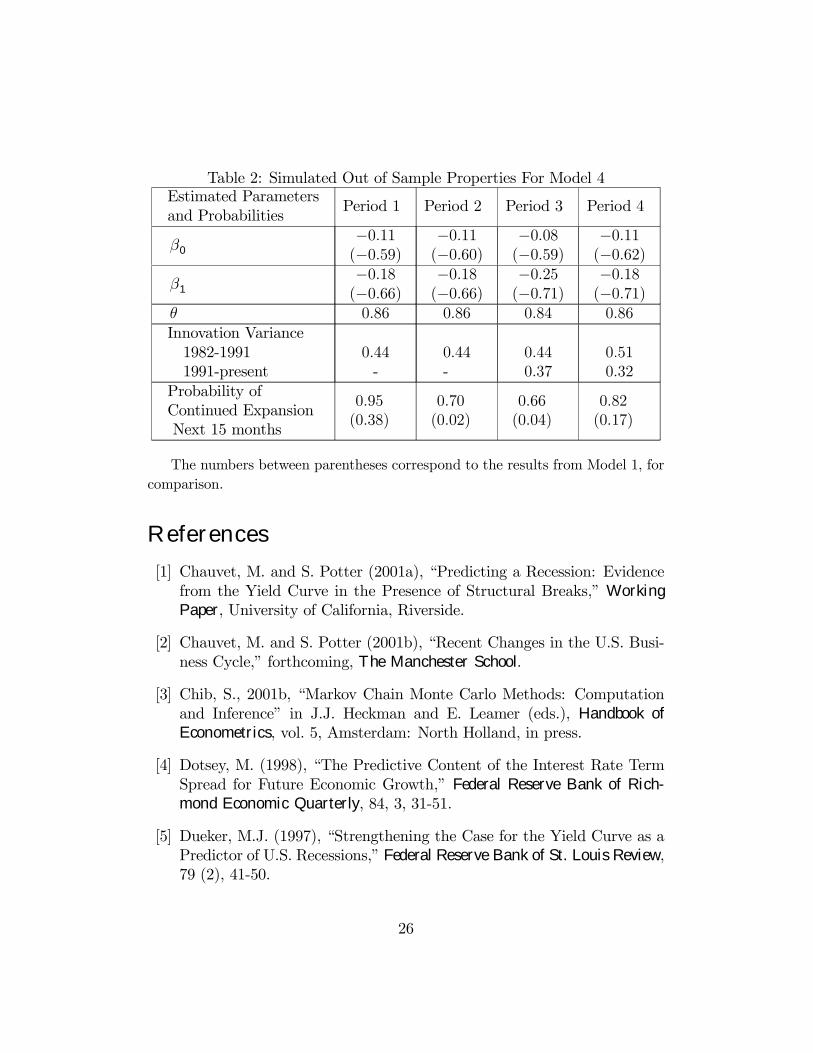
Notice that the first and third periods do not contain a recession, whilethe second period includes the 1990-91 recession. It is possible that the fourthperiod might contain a recession in its last two months.Table 2 contains some posterior features of this modified out-of-sample
forecasting exercise implemented for Model 4. The quantities in parenthesesrepresent the analogous results obtained using the original probit model ofEM (Model 1). The first thing to note is that the posterior means of theparameters are relatively stable across the estimation periods. The onlyminor exception is when the data from January 1999 to December 2000 isincorporated (i.e., moving from period 3 to period 4).With respect to the hitting probabilities, the probability of continuing
expansion from January 1999 to March 2000 is relatively low at 0.66. Al-though it is providing a stronger recession signal than period 2, it is not asstrong as the current prediction of 0.49 (Table 1). From Figure 1 we canobserve that the term spread was relatively low at the end of 1998, but thelack of a subsequent recession in 1999 leads to an attenuation of the effectof the spread compared to the constant term. On the other hand, the im-portance of the spread increases with the introduction of the 1990s into thesample, indicating that the large positive spreads for most of the period wereconsistent with the long expansion observed18.
17EM find that the in-sample results for the standard probit specification did not nec-essarily match with the out-of-sample performance. For the more complicated versionsconsidered here, the computational burden is too high to repeat the the comprehensiverecursive forecasting exercise conducted by these authors.18That is, the slope coefficient divided by the innovation standard deviation is substan-
tially larger in absolute value.
22
The model is relatively successful in forecasting the 1990-91 recession inthe sense that it did not produce a false signal in 1989. However, only a weakrecession signal is produced before the actual recession, as found by previousmodels. In particular, the probability of continuing expansion for period 2 is0.70. Notice that if we return to the recession forecast for the 1999 period,there was considerable speculation regarding the end of the expansion in theFall of 1998, given the financial turmoil experienced by Russia and fears offinancial contagion. These discussions were cut short with the strong growthof the US economy in the first quarter of 1999. Similar speculations weretaking place before the 1990 recession, but the strong economic growth inthe first quarter of 1990 also faded away discussions of a recession. However,in 1990 a recession hit the economy in the third quarter of the year.The performance of the EM model is similar to the more complicated
model in a qualitative sense. However, the standard probit model of EMgives hitting probabilities that are poorly calibrated. In particular, the pos-terior mean of the probability of continuing expansion from this model tendto be very low. Even for the prediction in period 1, which does not includea recession (but does include a slowdown), the upper 97.5% percentile of theprobability of a continuing expansion is only 0.5. Thus, the model is basi-cally signalling the 1989 slowdown. Given that generally slowdowns precederecessions, but not all slowdowns turn into recessions, this suggests that themore complicated probit model gives a more accurate quantitative evidenceon the likelihood of recession.
5 ConclusionsThis paper extends the probit specification of EM to account for the pos-sibility of multiple breakpoints and serially correlated errors. We use thealternative specifications to construct hitting probabilities to the next reces-sion. We find that a probit model with business cycle specific innovationvariance and an autoregressive component has a much better in sample fitthan the original probit model of EM. In particular, the recession forecastsfrom this more complicated model are very different from the ones obtainedfrom the standard probit specification. In addition, the hitting probabilitiessuggest substantial misspecification in the standard probit model of EM.All specifications considered indicate that the yield curve is signaling
weak future economic activity in 2000-2001. However, the strength of the
23
recession signals differs substantially across the specifications. The versionsof the probit model that do not correct for serially correlated errors displaythe highest posterior probability of a recession for 2001-2002. On the otherhand, the more sophisticated specifications that allow the latent variable tobe serially correlated lead to smaller probabilities of a recession in the nearfuture.
AppendixIn this appendix we derive the formula required for the Gibbs sampler drawsin the case of Model 4. First note that the full conditional distribution underthe first order autoregressive assumption
f(Y ∗t |Y ∗T , . . . , Y ∗t+1, Y∗
t−1, . . . , Y∗
K+1)
is equivalent to:
f(Y ∗t |Y ∗t+1, Y∗
t−1).
Since Y ∗t+1, Y∗
t , Y∗
t−1 has a joint normal distribution, the conditional distribu-tion is normal. Under the assumption that all initial values are zero, we canwrite the latent time series Y ∗t at time t as:
Y ∗t = eXt +t−K−1X
s=0
θsσ(t− s)εt−s.
Thus, the latent time series conditional on the yield is multivariate normalwith mean vector
h eXt+1, eXt, eXt−1
iand variance matrix: V (eYt+1) θV (eYt) θ2V (eYt−1)
θV (eYt) V (eYt) θV (eYt−)θ2V (eYt−1) θV (eYt−1) V (eYt−1)
.The results are then based on standard relationships between joint normalsand conditional normals.
24
Table 1: Posterior Means Across ModelsEstimated Parametersand Probabilities
The numbers between parentheses correspond to the results from Model 1, forcomparison.
References[1] Chauvet, M. and S. Potter (2001a), “Predicting a Recession: Evidence
from the Yield Curve in the Presence of Structural Breaks,” WorkingPaper, University of California, Riverside.
[2] Chauvet, M. and S. Potter (2001b), “Recent Changes in the U.S. Busi-ness Cycle,” forthcoming, The Manchester School.
[3] Chib, S., 2001b, “Markov Chain Monte Carlo Methods: Computationand Inference” in J.J. Heckman and E. Leamer (eds.), Handbook ofEconometrics, vol. 5, Amsterdam: North Holland, in press.
[4] Dotsey, M. (1998), “The Predictive Content of the Interest Rate TermSpread for Future Economic Growth,” Federal Reserve Bank of Rich-mond Economic Quarterly, 84, 3, 31-51.
[5] Dueker, M.J. (1997), “Strengthening the Case for the Yield Curve as aPredictor of U.S. Recessions,” Federal Reserve Bank of St. Louis Review,79 (2), 41-50.
26
[6] Estrella, A. and G. Hardouvelis (1991), “The Term Structure as a Pre-dictor of Real Economic Activity,” Journal of Finance, 46 (2), 555-576.
[7] Estrella, A. and F. S. Mishkin (1998), “Predicting U.S. Recessions: Fi-nancial Variables as Leading Indicators,” The Review of Economics andStatistics, 80, 45-61.
[8] Estrella, A., A.P. Rodrigues, and S. Schich (2000), “How Stable Is thePredictive Power of the Yield Curve? Evidence from Germany and theUnited States,” mimeo, Federal Reserve Bank of New York.
[9] Friedman, B.M. and K.N. Kuttner (1998), “Indicator Properties of thePaper-Bill Spread: Lessons from Recent Experience,” The Review ofEconomics and Statistics, 80, 34-44.
[10] Geweke, J., (1999), “Using Simulation Methods for Bayesian Economet-ric Models: Inference, Development and Communication,” EconometricReviews, 18, 1-126.
[11] Hamilton, J.D. and D.H. Kim, (2000), “A Re-Examination of thePredictability of Economic Activity Using the Yield Spread,” mimeo,UCSD.
[12] Harvey, C.R. (1989), “Forecasts of Economic Growth from the Bondand Stock Markets,” Financial Analysts Journal, 45 (5), 38-45.
[13] Haubrich, J.G. and A.M. Dombrosky (1996), “Predicting Real GrowthUsing the Yield Curve,” Federal Reserve Bank of Cleveland EconomicReview, 32 (1), 26-34.
[14] Jeffrey, H. (1961), Theory of Probability 3rd ed., Oxford: ClarendonPress.
[15] Kim, C-J. and C. Nelson (1999), “Has the U.S. Economy Become MoreStable? A Bayesian Approach Based on a Markov Switching Model ofthe Business Cycle,” Review of Economics and Statistics, 81(4) pp 1-10.
[16] Koop, G. and S. M. Potter (1999), “Bayes Factors and Nonlinearity:Evidence from Economic Time series,” Journal of Econometrics, 88,251-281.
27
[17] Laurent, R. (1989), “Testing the Spread,” Federal Reserve Bank ofChicago Economic Perspectives, 13, 22-34.
[18] McConnell, M. and G. Perez-Quiros (2000), “Output Fluctuations in theUnited States: What Has Changed Since the Early 1980s?” AmericanEconomic Review, 90, 5, 1464-1476.
[19] Neftci, S. (1996): An Introduction to the Mathematics of FinancialDerivatives, New York: Academic Press.
[20] Stock, J. and M. Watson (1989), “New Indices of Coincident and Lead-ing Indicators,” In O. Blanchard and S. Fischer edited NBER Macroe-conomic Annual Cambridge, MIT Press.
[21] Stock, J.H. and M.W. Watson (2000), “Forecasting Output and Infla-tion: The Role of Asset Prices,”mimeo, Kennedy School of Government,Harvard University.
28
29
- 4
- 3
- 2
- 1
0
1
2
3
4
5
5 5 6 0 6 5 7 0 7 5 8 0 8 5 9 0 9 5 0 0- 4
- 2
0
2
4
6
8
1 0
1 2
5 5 6 0 6 5 7 0 7 5 8 0 8 5 9 0 9 5 0 0
- 4
- 2
0
2
4
6
8
5 5 6 0 6 5 7 0 7 5 8 0 8 5 9 0 9 5 0 0- 4
0
4
8
1 2
5 5 6 0 6 5 7 0 7 5 8 0 8 5 9 0 9 5 0 0
F ig u r e 1 - N e g a t iv e P o s te r io r M e a n L a te n t V a r ia b le U n d e r D if f e r e n t A s s u m p t io n s (_ _ ) , A c t u a l Y ie ld C u r v e (S t - 1 2 ) ( - - - ) , a n d N B E R R e c e s s io n s (S h a d e d A r e a )
a ) M o d e l 1 - C o n s ta n t V a r ia n c e a n d i. i. d . E r r o r s b ) M o d e l 2 - C h a n g i n g V a r ia n c e a n d i. i. d . E r r o r s
c ) M o d e l 3 - C o n s ta n t V a r i a n c e a n d A R ( 1 ) P r o c e s s d ) M o d e l 4 - C h a n g in g V a r i a n c e a n d A R (1 ) P r o c e s s
30
0 . 0
0 . 2
0 . 4
0 . 6
0 . 8
1 . 0
5 5 6 0 6 5 7 0 7 5 8 0 8 5 9 0 9 5 0 0.0
.1
.2
.3
.4
.5
.6
.7
.8
.9
5 5 6 0 6 5 7 0 7 5 8 0 8 5 9 0 9 5 0 0
0 . 0
0 . 2
0 . 4
0 . 6
0 . 8
1 . 0
5 5 6 0 6 5 7 0 7 5 8 0 8 5 9 0 9 5 0 00 .0
0 .2
0 .4
0 .6
0 .8
1 .0
5 5 6 0 6 5 7 0 7 5 8 0 8 5 9 0 9 5 0 0
F ig u r e 2 - P o s t e r io r M e a n P r o b a b ili t i e s o f R e c e s s io n U n d e r D if fe r e nt A s s u m p t io n s , a nd N B E R R e c e s s io n s ( S h a d e d A r e a )
a ) M o d e l 1 - C o n s ta n t V a r i a n c e a n d i. i.d . E r r o r s b ) M o d e l 2 - C h a n g i n g V a r ia n c e a n d i. i. d . E r r o r s
c ) M o d e l 3 - C o n s t a n t V a r ia n c e a n d A R ( 1 ) P ro c e s s d ) M o d e l 4 - C h a n g in g V a r i a n c e a n d A R (1 ) P r o c e s s
31
0 .0
0 .2
0 .4
0 .6
0 .8
1 .0
0 .0
0 .2
0 .4
0 .6
0 .8
1 .0
0 .0
0 .2
0 .4
0 .6
0 .8
1 .0
0 .0
0 .2
0 .4
0 .6
0 .8
1 .0
F ig u r e 3 - P o s t e r io r M e a n F o r e c a s ts o f R e c e s s io n U n d e r D i f f e r e n t A s s u m p t io n s f o r 2 0 0 1 /2 0 0 2
a ) M o d e l 1 - C o n s t a n t V a r ia n c e a n d i .i. d . E r r o r s b ) M o d e l 2 - C h a n g i n g V a r ia n c e a n d i . i.d . E r r o r s
d ) M o d e l 4 - C h a n g i n g V a r i a n c e a n d A R (1 ) P r o c e s sc ) M o d e l 3 - C o n s t a n t V a r ia n c e a n d A R (1 ) P r o c e s s