Page 1
Munich Personal RePEc Archive
Forecasting the optimal order quantity in
the newsvendor model under a correlated
demand
Halkos, George and Kevork, Ilias
University of Thessaly, Department of Economics
4 February 2013
Online at https://mpra.ub.uni-muenchen.de/44189/
MPRA Paper No. 44189, posted 04 Feb 2013 12:29 UTC
Page 2
1
Forecasting the Optimal Order Quantity in the
Newsvendor Model under a Correlated Demand
George E. Halkos and Ilias S. Kevork Laboratory of Operations Research, Department of Economics,
University of Thessaly, Korai 43, Volos, Greece
Abstract
This paper considers the classical newsvendor model when, (a) demand is
autocorrelated, (b) the parameters of the marginal distribution of demand are
unknown, and (c) historical data for demand are available for a sample of successive
periods. An estimator for the optimal order quantity is developed by replacing in the
theoretical formula which gives this quantity the stationary mean and the stationary
variance with their corresponding maximum likelihood estimators. The statistical
properties of this estimator are explored and general expressions for prediction
intervals for the optimal order quantity are derived in two cases: (a) when the sample
consists of two observations, and (b) when the sample is considered as sufficiently
large. Regarding the asymptotic prediction intervals, specifications of the general
expression are obtained for the time#series models AR(1), MA(1), and ARMA(1,1).
These intervals are estimated in finite samples using in their theoretical expressions,
the sample mean, the sample variance, and estimates of the theoretical autocorrelation
coefficients at lag one and lag two. To assess the impact of this estimation procedure
on the optimal performance of the newsvendor model, four accuracy implication
metrics are considered which are related to: (a) the mean square error of the
estimator, (b) the accuracy and the validity of prediction intervals, and (c) the actual
probability of running out of stock during the period when the optimal order quantity
is estimated. For samples with more than two observations, these metrics are
evaluated through simulations, and their values are presented to appropriately
constructed tables. The general conclusion is that the accuracy and the validity of the
estimation procedure for the optimal order quantity depends upon the critical fractile,
the sample size, the autocorrelation level, and the convergence rate of the theoretical
autocorrelation function to zero.
Keywords: Newsvendor model; accuracy implication metrics; time#series models;
prediction intervals; Monte#Carlo simulations.
JEL Codes: C13; C22; C53; M11; M21.
Page 3
2
1. Introduction
In the majority of papers in stock control, the optimal inventory policies are
derived under two conditions: (a) the parameter values of the stochastic law which
generates the demand are known, and (b) the demand in successive periods is formed
independently. In practice, the first condition does not hold. One solution to this
problem is the substitution of the true moments of the demand distribution in the
theoretical formulae determining the target inventory measures with values which are
obtained through certain estimation procedures (e.g. Syntetos & Boylan, 2008;
Janssen et al., 2009). Then, in the context of managerial aspects of inventories, the
combined estimation – stock control operation should be evaluated through specific
accuracy implication metrics which are usually related to service levels and inventory
costs (Boylan & Syntetos 2006; Syntetos et al., 2010).
Regarding the second condition, for the last three decades, an increasing
number of works has been starting to appear in the literature aiming to study the
effect of a serially correlated demand on the behavior of target inventory measures in
stock control and supply chain management (Zhang, 2007). In this context, a variety
of time#series models, including ARIMA processes and linear state space models
(Aviv, 2003), have been used to describe the evolution of demand. Adopting these
time#series demand models, the research has been expanded to resolve several
problems in inventory management including the determination of safety stocks and
optimal policies in continuous and periodic review systems, as well as, the study of
the bullwhip effect and the value of information sharing.
For the classical newsvendor model, the research on determining the order
quantity when the demand in successive periods is autocorrelated and the parameters
of demand distribution are unknown is very limited. Although a number of works
Page 4
3
offer solutions to the problem of not knowing the parameters of demand distribution
(e.g. Ritchken & Sankar, 1984; Liyanage & Shanthikumar, 2005; Kevork, 2010,
Akcay et al., 2011; Halkos & Kevork, 2012a), these works assume that demand in
successive periods is formed independently. To the extent of our knowledge, the work
of Akcay et al. (2012) is the only one which addresses in the classical newsvendor
model the issues of both the correlated demand and the demand parameters
estimation. In particular, using a simulation#based sampling algorithm, this work
quantifies the expected cost due to parameter uncertainty when the demand process is
an autoregressive#to#anything time series, and the marginal demand distribution is
represented by the Johnson translation system with unknown parameters.
In the current paper, we study the classical newsvendor model (e.g. Silver et
al., 1998; Khouja, 1999) when it operates under optimal conditions, and the demand
for each period (or inventory cycle) is generated by the non#zero mean linear process
with independent normal errors which have zero mean and the same variance.
Assuming that historical data on demand are available for the most recent �
successive periods, we determine for period �� + the order quantity, by replacing in
the theoretical expression which holds under optimality the unknown true stationary
mean and the unknown true stationary variance with their corresponding Maximum
Likelihood (ML) estimates.
This process leads to deviations between the computed order quantity and the
corresponding optimal one. These deviations are not systematic since they are caused
by the variability of the sample mean and the sample variance. Therefore, we
consider the computed order quantity as an estimate for the optimal order quantity.
This estimate belongs to the sampling distribution of the estimator which has been
constructed after replacing in the theoretical expression (which gives the optimal
Page 5
4
order quantity) the true mean and the true variance with their corresponding ML
estimators.
The distribution of this estimator for the optimal order quantity is derived for
�� = and when � is sufficiently large. Then, general expressions of the exact (for
�� = ) and the asymptotic prediction interval for the optimal order quantity are
obtained. Regarding the exact prediction interval, apart from the sample mean and the
sample variance, its formula contains also the theoretical autocorrelation coefficient
at lag one. Using the estimate of this coefficient, we take the corresponding estimated
exact prediction interval whose performance is evaluated for different autocorrelation
levels over a variety of choices for the critical fractile. The latter quantity is the
probability not to experience a stock out during the period when the newsvendor
model operates at optimal conditions. Although the case of �� = could be considered
as an extreme case, and possibly not realistic, the examination of the properties of the
exact prediction interval for such a very small sample size gives considerable insights
in the process of estimating the optimal order quantity. Besides, as it will be clearer
below, it is too difficult to give for �� > analogous general expressions for exact
prediction intervals.
As it is not possible to obtain exact prediction intervals for any �� > , to carry
on with the estimation of the optimal order quantity at any finite sample, we use the
general expression of the asymptotic prediction interval. To evaluate its performance
in finite samples, we consider three special cases of the linear process, which are the
time#series models AR(1), MA(1), and ARMA(1,1). For each model, the
specification of the general expression of the asymptotic prediction interval is
obtained. In the models AR(1) and MA(1), the specified formula contains, apart from
the sample mean and the sample variance, the unknown true variance and the
Page 6
5
theoretical autocorrelation coefficient at lag one. The corresponding formula in the
ARMA(1,1) includes also the theoretical autocorrelation coefficient at lag two.
Replacing the variance and the two autocorrelation coefficients with their
corresponding sample estimates, we get the estimated prediction intervals whose
performance is also evaluated for different sample sizes and again for different
autocorrelation levels over a variety of choices for the critical fractile.
To assess the impact of the aforementioned estimation procedure for the order
quantity on the optimal performance of the newsvendor model, we consider four
accuracy implication metrics which are related to:
(a) the accuracy of the prediction intervals,
(b) the validity of the prediction intervals,
(c) the mean square error of the estimator of the optimal order quantity, and
(d) the actual probability not to have a stock#out during the period when the
optimal order quantity is estimated.
Exact values for the four metrics are obtained for �� = . For larger sample
sizes, the metrics are obtained through Monte Carlo simulations. The values of these
four metrics enable us to trace at different autocorrelation levels the minimum
required sample size so that the estimation procedure to have a negligible impact on
the optimal performance of the newsvendor model.
To derive the prediction intervals for the optimal order quantity, we studied
the conditions under which the sample mean and the sample variance are
uncorrelated and independent. For the general ARMA model, Kang and Goldsman
(1990) showed that the correlation between the sample mean and several variance
estimators is zero. These variance estimators are based on the techniques of the non#
overlapping/overlapping batched means and the standardized time series. Bayazit et
Page 7
6
al. (1985) offered an expression for the covariance of the sample mean and the
sample variance of a skewed AR(1).
Extending these findings, we prove in our work two further results. First, for
any sample with two observations being drawn from the general linear process with
independent normal errors, which have zero mean and constant variance, the sample
mean and the sample variance are independent. Second, for the same linear process,
when the theoretical autocorrelation function is positive and the autocorrelation
coefficients are getting smaller as the lag increases, in any sample with more than two
observations, the sample mean and the sample variance are uncorrelated but not
independent.
Given the above arguments and remarks, the rest of the paper is organized as
follows. In the next section we give a brief literature review of studies which adopted
time series models to describe the evolution of demand in continuous review and
periodic review inventory systems. In section 3 we present the newsvendor model
with the demand in each period to follow the non#zero mean linear process, and we
derive the theoretical expression which determines the optimal order quantity. In
section 4 we derive the general expressions of the exact for �� = and the asymptotic
prediction interval for the optimal order quantity. The evaluation of the estimated
prediction intervals is performed and presented in section 5. Finally, section 6
concludes the paper summarizing the most important findings.
�
2. A brief review of the relevant literature
In the context of continuous review systems, the AR(1) and MA(1) processes
have been adopted as demand models for studying customer service levels and
deriving safety stocks and reorder points. Zinn et al. (1992) explained and quantified
Page 8
7
through simulations the effect of correlated demand on pre#specified levels of
customer service when lead#time distribution is discrete uniform. Fotopoulos et al.
(1988) offered a new method to find an upper bound of the safety stock when the lead
time follows an arbitrary distribution. Ray (1982) derived the variance of the lead#
time demand under fixed and random lead times when the parameters of the AR(1)
and MA(1) are known, and when the expected demand during lead time is forecast.
With fixed lead times, Urban (2000) derived variable reorder levels using for the
demand during lead time appropriate forecasts and time#varying forecast errors
variance/covariance, which are updated every period conditional upon the most recent
observed demand.
For periodic review systems, Johnson and Thompson (1975) showed that
when demand is generated by the stationary general autoregressive process, the
myopic policy for the one period is optimal for any period of an infinite time horizon.
To prove it they showed that in any period it is always possible to order up to the
optimal order quantity. Assuming that demand is normal and covariance#stationary
with known autocovariance function, Charnes et al. (1995) derived the safety stock
required to achieve the desired stock#out probability with an order#up#to an initial
inventory level. Urban (2005) developed a periodic review model when demand is
AR(1) and depends on the amount of inventory displayed to the customer. Zhang
(2007) quantified the effect of a temporal heterogeneous variance on the performance
of a periodic review system using an AR(1) and a GARCH(1,1) to describe the
dynamic changes in the level and the variance of demand respectively. Adopting the
ARIMA (0,1,1) as the demand generating process in a periodic review system,
Strijbosch et al. (2011) studied the effect of single exponential smoothing and simple
moving average estimates on the fill rate conducting appropriate simulations.
Page 9
8
Apart from the classical continuous and periodic review systems, there are
also other active research areas on inventories where time series processes have been
adopted as demand models. For instance, Zhang (2007) provides a list of works
which use time series models to study the bullwhip effect, the value of information
sharing, and the evolution of demand in supply chains. Ali et al. (2011) also provide a
relevant literature for those works which by adopting time series processes as demand
models explore the interaction between forecasting performance and inventory
implications.
3. Background
Suppose that the demand size for period t (or inventory cycle t) of the classical
newsvendor model is generated by the non# zero mean linear process
∑∞
=−εψ+=
0k
ktjtY , (1)
where ∞<ψ∑∞
=0k k , and tε s are independent normal variables with ( )2εσ0ε ,N~t .
Denote also by tQ the order quantity for period t, � the selling price, � the purchase
cost per unit, � the salvage value, and � the loss of goodwill per unit of product. To
satisfy the demand of period t, the newsvendor has available stock at the start of the
period only the order quantity tQ . This means that any excess inventory at the end of
period 1−t was disposed of through either consignment stocks or buyback
arrangements and the salvage value was used to settle such arrangements. Further, by
receiving this order quantity, no fixed costs are charged to the newsvendor.
Under the aforementioned notation and assumptions, and providing that the
coefficient of variation of the marginal distribution of tY is not large (e.g. see Halkos
Page 10
9
and Kevork, 2012b), the expected profit of the newsvendor at the end of period t is
derived from expression (1) of Kevork (2010) and is given by
( ) ( ) ( ) ( )[ ] ( )+≥−≥−−−−−=π 0YQPr0YQ YEQvpQcpE tttttttt
( )[ ] ( )0YQPr0YQ YEQs tttttt <−<−−+ .
Let ( )zϕ and ( )zΦ be respectively the probability density function and the
distribution function of the standard normal evaluated at ( ) otQz γ−= , where oγ
is the variance of the marginal distribution of tY . Since
( ) ( ) ( )zQPr0YQPr t0k ktktt Φ=−≤εψ=≥− ∑∞
= − ,
( ) ( )=−≤εψεψ+=≥− ∑∑∞
= −
∞
= − t0k ktk0k ktkttt Q E0YQ YE
( )( )z
zQ ZZE o
o
to Φ
ϕγ−=
γ
−≤γ+= ,
and
( ) ( )( )z1
zQ ZZE0YQ YE o
o
tottt Φ−
ϕγ+=
γ
−>γ+=<− ,
the expected profit becomes
( ) ( ) ( ) ( ) ( ) ( ) ( ){ }otttt zzQsvpQsQcpE γϕ+Φ−+−−−+−=π .
The first and second order conditions obtained by differentiating ( )tE π with respect
to tQ are
( ) ( ) ( ) ( ) 0zsvpscpdQ
dE
t
t =Φ+−−+−=π
and
( ) ( ) ( )0
zscp
dQ
Ed
o
2
t
t
2
<γ
ϕ+−−=
π.
Page 11
10
Setting ( ) ( )svpscpR +−+−= , the first order condition leads to the
following equation, which is known as the ctitical fractile equation,
( ) ( ) Rsvp
scpzZPrQYPr R
*
ttzR=
+−+−
=≤=≤=Φ ,
where R is the critical fractile, *
tQ is the optimal order quantity, and
( ) o
*
tR Qz γ−= . Thus the optimal order quantity for period t is determined from
oR
*
t zQ γ+= . (2)
In the classical newsvendor model, no stock is carried from previous periods
to the current. So, for a time horizon consisting of a number of periods, if the
distribution of demand in each period remained the same with the same mean and the
same variance, the optimal order quantity would depend upon only the critical fractile
R. And R is function of the overage and underage costs. In the analysis which
follows, to simplify notations and symbols, we shall assume that in each period of the
time horizon for which demand data are available, the critical fractile does not
change. Thus for each period of the time horizon, the optimal order quantity remains
the same, and so it is legitimate to drop out the subscript t from the symbol of the
optimal order quantity.
4. Prediction intervals for the optimal order quantity ��
Suppose that the linear process given in (1) has generated the realization
nY,...,Y,Y 21 , which represents demand for the most recent n successive periods in
the newsvendor model. Further, let nYYn
1t t∑ == and ( )2
1ˆ
�
� ��� � �γ
== −∑ be ML
estimators of and oγ respectively. Since in practice and oγ are unknown
Page 12
11
quantities, replacing the ML estimators into (2), in the places of and oγ , the
resulting estimator for the optimal order quantity takes the form�
( ) oRo
* ˆzYˆ,YQ̂ γ+=γ= � . (3)
Given the estimator *Q̂ , the rest of this section is organized as follows. At
first, we derive the general expression for the exact prediction interval for *Q when
the sample consists of two observations. On the other hand, it is too difficult to give
for 2n > analogous general expressions for the exact prediction interval for two
reasons. The first is that the sample variance consists of correlated chi#squared
random variables and the second reason is that, as we shall show later, for the time
series models AR(1), MA(1), and ARMA(1,1), the sample mean and the sample
variance are not independent.
Despite the dependency of the sample mean and the sample variance, in the
second part of this section we prove that for any 2n > their covariance is zero. So,
with the asymptotic distributions of Y and oγ̂ to be available in the literature, this
allows us to construct the asymptotic variance#covariance matrix of Y and oγ̂ , and
then, by applying the multivariate Delta method, to derive the general expression of
the asymptotic distribution of *Q̂ .
���� �������������������� ������ �� ������ �� = �
If tY is determined by the linear process given in (1) with ∞<ψ∑∞
=0k k and
tε ’s to be i.i.d. normal random variables with zero mean and constant variance, the
sample 1Y , 2Y follows the bivariate normal with marginal mean and variance oγ .
In this case, 2
o Xˆ =γ , where ( ) 2YYX 21 −= , with ( ) 0XE = , ( ) ( ) 21XVar 1o ρ−γ=
and 1ρ to be the autocorrelation coefficient at lag one. Then the statistic
Page 13
12
( )1o 1X2 ρ−γ follows the standard normal, and hence ( ) 2
1o1o ~1ˆ2 χγρ−γ . It
also holds that the sample mean ( ) 2YYY 21 += is normally distributed with mean
and variance ( ) 21 1o ρ+γ .
Proposition 1: If 1Y , 2Y is a sample drawn from the linear process given in (1),
with ∞<ψ∑∞
=0k k , and tε ’s to be i.i.d. random variables with ( )2εσ0ε ,N~t , then
Y and oγ̂ are distributed independently.
Proof: See in the appendix.
Using the result of proposition 1, together with the distributions of Y and oγ̂ ,
for 2n = we derive the following statistic
( )( )
( )
( )λ′γ
−ρ+
ρ−=
γρ−
γ
ρ+−+
ρ+γ
−
=′ 1
o
*
1
1
o1
o
1
R
1ot~
ˆ
QY
1
1
1
ˆ2
1
2z
1
Y2
T , (4)
where ( )λ′1t is the non#central student#t distribution with one degree of freedom and
non#centrality parameter
1
R1
2z
ρ+−=λ . (5)
So the interval
( ) ( )
ρ−
ρ+γλ′−
ρ−
ρ+γλ′− αα
−1
1o
2,1
1
1o
21,1 1
1ˆtY ,
1
1ˆtY (6)
is the exact ( ) %1001 α− prediction interval (P.I.) for *Q for the special case where
2n = �
Page 14
13
��� ���� The exact distribution of oγ̂ for 2n = allows the exact computation of the
Bias of *
tQ̂ . The statistic ( )[ ]1oo 1ˆ2 ρ−γγ follows the chi#distribution with one
degree of freedom, and so we have ( ) ( ) πρ−γ=γ 1oo 1ˆE and
( ) ( )
−
πρ−
γ=−= 11
zQQ̂EQ̂Bias 1oR
*** .
The expression within the parentheses containing 1ρ and π is always negative. So, for
any 5.0R < the �� of *Q̂ is positive, while for 5.0R > the �� is negative.
��� ����� To evaluate the performance of the exact P.I. of (6), we define its relative
expected half#length (REHL) as
( ) ( )( )
( ) ( )
( )R
1
2,1
21,1
1o*
2,1
21,1
1
1
zCV2
tt1
ˆEQ2
tt
1
1REHL
+
λ′−λ′
πρ+
=γ
λ′−λ′
ρ−ρ+
=−
αα−
αα−
, (7)
where γ= oCV is the coefficient of variation, and *Q is given in (2). Dividing by
*Q ensures the comparability of REHLs evaluated at different Rs, since increasing the
critical fractile R, we get larger optimal order quantities.
Figure 1 illustrates the graph of the REHL versus R for different values of CV
and .1ρ . The choice of values for .1ρ is explained in the next section. By setting also
the maximum CV at 0.2, we avoid to take a negative demand (especially in the
simulations which are described in the next section), as we give a negligible
probability (less than 0.00003%) to take a negative value from the marginal
distribution of tY . Finally, the critical values of the non#central t were obtained
through the statistical package MINITAB.
Page 15
14
Figure 1: Graph of REHL as a function of R; n=2 and nominal confidence level 95%.
CV=0.05 CV=0.2
Looking at the two graphs of Figure 1, we first observe the increase of the
REHL as R is getting closer either to zero or to one. Given CV and R, as .1ρ increases
the REHL is also increasing, while given .1ρ and R, a higher CV results in larger
REHLs. Finally, we observe that as CV is getting larger, the minimum of REHL is
slightly shifted to the right of R=0.5.
������������������������������� ������� �� �
To derive the asymptotic distribution of *Q̂ , we shall use the asymptotic
distributions of Y and oγ̂ stated in Priestley (1981, pp. 338, 339). Especially, when
demand follows the non#zero mean linear process given in (1) with ∞<ψ∑∞
=0k k ,
and tε ’s to be independent normal variables with zero mean and constant variance, it
holds that,
(a) ( )−Yn has a limiting normal distribution with zero mean and variance
∑+∞
−∞=
ργk
ko , and
(b) ( )ooˆn γ−γ is asymptotically normal with mean zero and variance ∑
+∞
−∞=
ργk
2
k
2
o2 ,
where kρ is the autocorrelation coefficient at lag k.
Page 16
15
Proposition 2: Let nY,...,Y,Y 21 be a sample drawn from the linear process given in
(1) with ∞<ψ∑∞
=0k k , and tε ’s to be i.i.d. random variables with ( )2εσ0ε ,N~t .
Then, for any sample size the covariance of the sample mean and the sample variance
is zero.
Proof: See in the appendix.
The result of proposition 2, together with the asymptotic distributions of Y
and oγ̂ lead us to state that
( ) , Nˆˆ
Yn 2
oo
Σ0→
γ−γ
− �,
where
ργ
ργ
=
∑
∑
∞+
−∞=
+∞
−∞=
k
2
k
2
o
k
ko
20
0
Σ ,
“�” stands for convergence in distribution, and N2 is the bivariate normal
distribution. It also holds that
( ) *
oR
5.0
oR
* QzˆlimpzYQ̂limp =γ+=γ+= �� .
So, by applying the multivariate Delta Method (e.g. Knight, 2000 pp. 149) we take
( ) ( ){ } ( ) ( ) , NQQ̂n,ˆ,Yn **
oo LΣL0 ⋅⋅′→−=γ−γ ��� ,
γ=
γ∂∂
∂∂
=′
γ=γ=
γ=γ=
o
R
ˆYoˆ
Y 2
z1
ˆYoooo
��L ,
and
ρ+ργ=⋅⋅′ ∑∑∞+
−∞=
∞+
−∞= k
2
k
2
R
k
ko2
z LΣL .
Thus,
Page 17
16
( ) ( )1,0N
2
z
QQ̂n
k
2
k
2
R
k
ko
**
→
ρ+ργ
−
∑∑∞+
−∞=
∞+
−∞=
� , (8)
and so the asymptotic ( ) %1001 α− prediction interval for *Q will have the form
ρ+ρ
γ± ∑∑
∞+
−∞=
∞+
−∞=α
k
2
k
2
R
k
ko
2
*
2
z
nzQ̂ . (9)
�� ������ Consider the stationary AR(1) model given by ( ) t1tt YY ε+−φ+= − ,
where 1<φ , ( )22
o 1 φ−σ=γ ε , and k
k φ=ρ (k=0, 1, 2,…). Considering that the
process has been started at some time in the remote past, and substituting repeatedly
for 1tY − , 2tY − , 3tY − , …, the AR(1) takes the form of process (1) with j
j φ=ψ . Then
we have
φ−φ+
=φ−φ
+=ρ+=ρ ∑∑∞
=
∞
−∞= 1
1
1
2121
0k
k
k
k
and
2
2
2
2
0k
2
k
k
2
k1
1
1
2121
φ−
φ+=
φ−
φ+=ρ+=ρ ∑∑
∞
=
∞
−∞=
.
Hence the asymptotic prediction interval for *Q is specified as
ρ−
ρ++
ρ−
ρ+γ± α 2
1
2
1
2
R
1
1o2
*
1
1
2
z
1
1
nzQ̂ , (10)
since φ=ρ1 .
�� ����� �� Consider the invertible MA(1) model, 1tttY −θε+ε+= , with 1<θ ,
( )22
o 1 θ+σ=γ ε , ( )2
1 1 θ+θ=ρ , and 0k =ρ for 2k ≥ . This model takes the form of
process (1) by setting 1o =ψ , θ=ψ1 , and 0k =ψ for 2k ≥ . Hence we take
Page 18
17
1
k
k 21 ρ+=ρ∑∞
−∞=
, 2
1
k
2
k 21 ρ+=ρ∑∞
−∞=
, and so the asymptotic prediction interval for *Q is
given by ( )
ρ++ρ+
γ± α
2
1
2
R1
o2
* 212
z21
nzQ̂ . (11)
��� ����� � Consider the stationary and invertible ARMA(1,1) model which is given
by ( ) 1tt1tt YY −− θε+ε+−φ+= , 1<φ , 1<θ , 2
2
2
o1
21εσφ−
φθ+θ+=γ ,
( )( )φθ+θ+
θ+φφθ+=ρ
21
121 , and 1
1k
k ρφ=ρ − for 2k ≥ . Given that the process has been
started at some time in the remote past, Harvey (1993, pp. 26) shows that this model
takes the form of process (1) with 1o =ψ , θ+φ=ψ1 , and 1kk −φψ=ψ for 2k ≥ .
Thus, we take ( )φ−ρ+=ρ∑∞
−∞=
121 1
k
k and ( )22
1
k
2
k 121 φ−ρ+=ρ∑∞
−∞=
. So the
asymptotic prediction interval for *Q is specified as
ρ−ρ
ρ++
ρ−ρ
ρ+
γ± α 2
2
2
1
4
1
2
R
21
2
1o
2
* 21
2
z21
nzQ̂ , (12)
after replacing φ by the ratio 12 ρρ .
We are closing this section by noting that for the three aforementioned time
series models and for 2n > the sample mean and the sample variance are not
independent random variables. This is proved in proposition 3. So, it is required these
intervals to be evaluated when they are applied to finite samples after replacing oγ ,
1ρ and 2ρ with their sample estimates. The results from this exercise and the relevant
discussion are given in the next section.
Page 19
18
Proposition 3: Let nY,...,Y,Y 21 be a sample from the linear process given in (1) with
∞<ψ∑∞
=0k k , and tε ’s to be i.i.d. random variables with ( )2εσ0ε ,N~t . Suppose
also that appropriate values are assigned to the jψ ’s weights such that
1...0 12n1n <ρ<<ρ<ρ≤ −− . Then for any 2n > , the ML estimators Y and oγ̂ are
not independent.
Proof: See in the appendix.
�
5. Prediction Interval Estimation
In this section we assess the performance of prediction intervals (6) and (9)
when the demand in each period of the newsvendor model is generated by the three
time#series models AR(1), MA(1), and ARMA(1,1). The evaluation is performed
over a variety of values for the critical fractile R, and choices of number of
observations in the sample n, when in the expressions (6), (10), (11) and (12) the
unknown population parameters are replaced respectively with the sample mean Y ,
the sample variance oγ̂ , and the estimates of the theoretical autocorrelation
coefficients 1ρ and 2ρ , which are obtained from (e.g. see Harvey, 1993, page 11)
( )( )
( )∑
∑
=
+=−
−
−−=
γ
γ=ρ
k
1t
2
t
n
1kt
ktt
o
kk
YY
YYYY
ˆ
ˆˆ .
For ease of exposition we divided this section into three parts. In the first part,
we justify the choice of the parameter values for the three models, describe the
evaluation criteria, and present the process of generating different realizations (or
replications) for each model through Monte#Carlo simulations. In the second part, we
derive and present some exact results for the evaluation criteria when the sample
Page 20
19
consists of only two observations. Finally, in the third part, we present and discuss
simulation results for the evaluation criteria, which are computed for different sample
sizes drawn from the generated replications of each model.
!�"���#������������������� ���� �������
The choice of values for the parameters φ , θ and 2
εσ of the three models
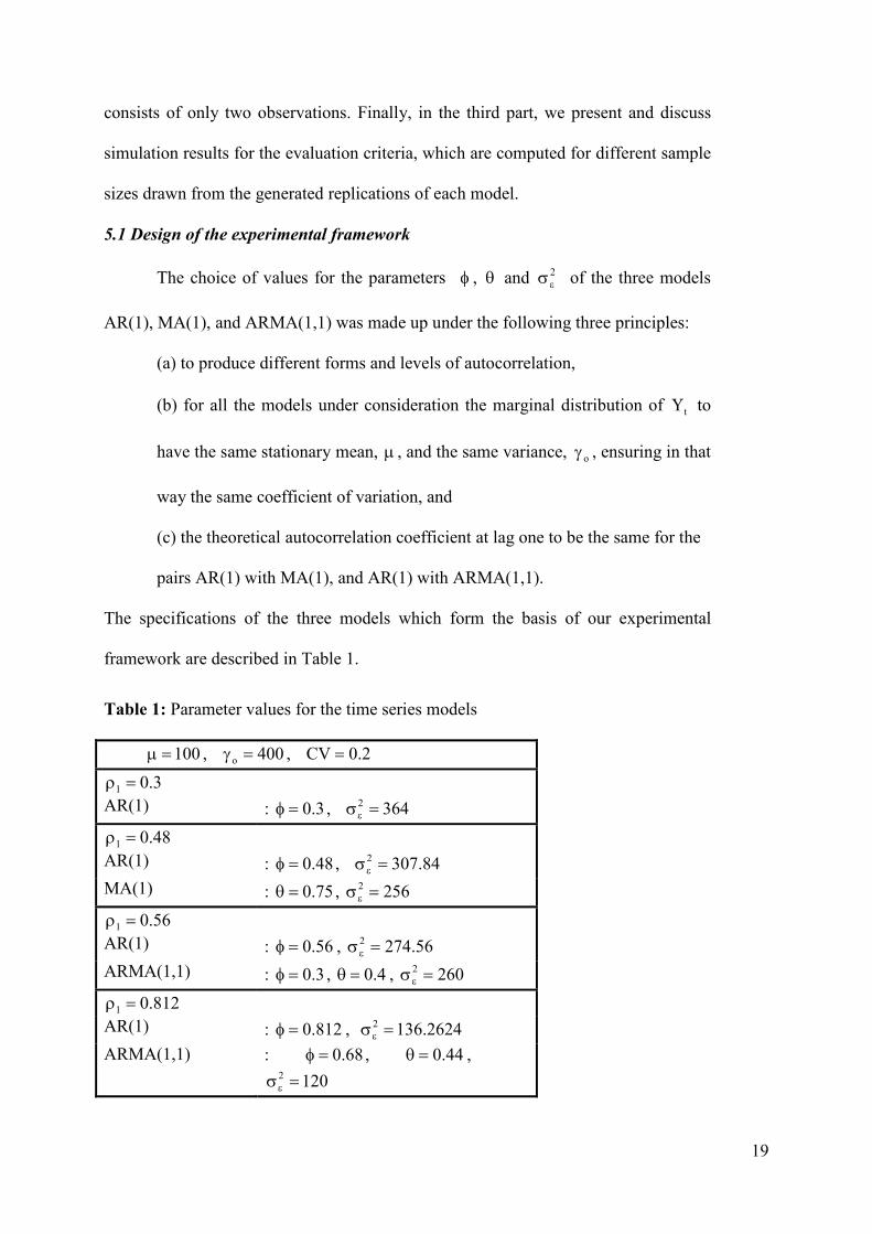
AR(1), MA(1), and ARMA(1,1) was made up under the following three principles:
(a) to produce different forms and levels of autocorrelation,
(b) for all the models under consideration the marginal distribution of tΥ to
have the same stationary mean, , and the same variance, oγ , ensuring in that
way the same coefficient of variation, and
(c) the theoretical autocorrelation coefficient at lag one to be the same for the
pairs AR(1) with MA(1), and AR(1) with ARMA(1,1).
The specifications of the three models which form the basis of our experimental
framework are described in Table 1.
Table 1: Parameter values for the time series models
100= , 400o =γ , 2.0CV =
3.01 =ρ
AR(1) : 3.0=φ , 3642 =σε
48.01 =ρ
AR(1) : 48.0=φ , 84.3072 =σε
MA(1) : 75.0=θ , 2562 =σε
56.01 =ρ
AR(1) : 56.0=φ , 56.2742 =σε
ARMA(1,1) : 3.0=φ , 4.0=θ , 2602 =σε
812.01 =ρ
AR(1) : 812.0=φ , 2624.1362 =σε
ARMA(1,1) : 68.0=φ , 44.0=θ ,
1202 =σε
Page 21
20
After replacing in (6), (10), (11), (12), the population parameters , oγ , 1ρ
and 2ρ by their corresponding sample estimates, the performance of the estimated
prediction intervals is assessed through four Accuracy Implication Metrics (AIM).
The first AIM is the actual probability the estimated prediction interval to include (or
otherwise to cover) the unknown population parameter which in our case is the
optimal order quantity *Q . We call this actual probability as coverage (CVG). The
next two AIMs are related to the precision of the estimated prediction intervals.
Particularly, we consider the Relative Mean Square Error (RMSE) of the estimator
*Q̂ and the relative expected half length (REHL) of the prediction interval for *Q .
These two metrics are computed by dividing respectively the mean square error and
the expected half#length of the interval by *Q . The justification of dividing by *Q
has been already explained in the previous section.
The last AIM is related to the actual probability actR not to experience a
stock#out during the period. The use of this metric is imposed since by replacing in
(2) the unknown quantities , oγ with their corresponding estimates, it is very likely
the order quantity to differ from *Q . Then, when the newsvendor model operates at
the optimal situation, the probability of not experiencing a stock#out during the period
is not equal to the critical fractile R. The last AIM, therefore, gives the difference
actRR − .
For the time series models of Table 1, we showed in the previous section that
for any 2n > , Y and oγ̂ are not independent. Due to the dependency of Y and oγ̂ ,
it is extremely difficult, or even impossible, to derive for 2n > the exact distribution
of the estimator *Q̂ , and so to obtain exact values for the four aforementioned AIMs.
To overcome this problem, we organized and conducted appropriate Monte#Carlo
Page 22
21
Simulations. In particular, for each model of Table 1, 20000 independent replications
of maximum size 2001 observations were generated. To achieve stationarity in each
AR(1) and ARMA(1,1), oY was generated from the stationary distribution ( )o,N γ ,
with 100= and 400o =γ . These values for and oγ were also used in the MA(1).
Furthermore, in each replication of ARMA(1,1) and MA(1), oε was generated
from the distribution ( )2,0N εσ , with the values of 2
εσ to be given in Table 1. We
found out that with oε randomly generated, for 2n = , the simulated results for the
CVG and the REHL were very close to the corresponding exact ones. On the
contrary, starting each replication with 0o =ε , the observed discrepancies among
simulated and exact results of CVGs and REHLs were considerable.
For each model of Table 1, and in each one of the 20000 replications, the
estimates Y , oγ̂ , 1ρ̂ and 2ρ̂ were obtained for different combinations of values of R
and sample sizes n. Then, in each replication, having available these four estimates,
for each combination of R and n, *Q̂ was computed using formula (2), and the
corresponding prediction interval was constructed using respectively (10), (11), (12),
after replacing in the variance of *Q̂ the unknown quantities oγ , 1ρ and 2ρ with their
corresponding estimates.
Using, therefore, for each model and for each combination of R and n, the
20000 different estimates from *Q̂ , and the 20000 different estimated prediction
intervals for *Q , the four AIMs were obtained as follows:
(a) The CVG was computed as the percentage of the 20000 prediction
intervals which included *Q .
Page 23
22
(β) The REHL was obtained dividing the average half#length of the 20000
prediction intervals by *Q .
(c) For the RMSE, first we computed the MSE as the sum of the variance of
the 20000 estimates from *Q̂ plus the squared of the difference of the average
of the 20000 estimates from *Q̂ minus *Q . Then the RMSE was computed
dividing the MSE by *Q .
(d) The difference actRR − was obtained by computing actR as the percentage
of the estimates from *Q̂ which were greater than the corresponding 1nY +
values.
Finally, let us mention that the random number generator which was used in
this study is described in Kevork (2010), while details about its validity are found in
Kevork (1990). To generate values from the normal distribution, we adopted the
traditional method of Box and Muller which is described in Law (2007).
�
!���� ������$��������%&'� �����()������ �� =
For 2n = , the estimate of 1ρ is
5.0
2
YYY
2
YYY
2
YYY
2
YYY
ˆ2
212
2
211
211
212
1 −=
+−+
+−
+−
+−
=ρ .
The lack of variability in 1ρ̂ when 2n = allows the exact computation of the CVG
and the REHL. The process of obtaining the exact results for these two metrics is
illustrated below.
Page 24
23
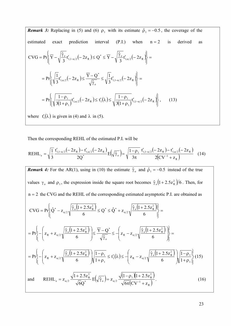
��� ��� � Replacing in (5) and (6) 1ρ with its estimate 5.0ˆ1 −=ρ , the coverage of the
estimated exact prediction interval (P.I.) when 2n = is derived as
( ) ( ) =
−′γ
−≤≤−′γ
−= αα− R2,1o*
R21,1o z2t
3
ˆYQz2t
3
ˆYPrCVG
( ) ( ) =
−′≤γ
−≤−′= α−α R21,1
o
*
R2,1 z2t3
1
ˆ
QYz2t
3
1Pr
( )( ) ( )
( )( )
−′ρ+
ρ−≤λ′≤−′
ρ+
ρ−= α−α R21,1
1
11R2,1
1
1 z2t13
1tz2t
13
1Pr , (13)
where ( )λ′1t is given in (4) and λ in (5).
Then the corresponding REHL of the estimated P.I. will be
( ) ( ) ( ) ( ) ( )( )R
1
R2,1R21,11o*
R2,1R21,1
ezCV2
z2tz2t
3
1ˆE
Q2
z2tz2t
3
1REHL
+
−′−−′
π
ρ−=γ
−′−−′=
−
αα−αα− (14)
��� ����� For the AR(1), using in (10) the estimate oγ̂ and 5.0ˆ1 −=ρ instead of the true
values oγ and 1ρ , the expression inside the square root becomes ( ) 6z5.21ˆ 2
Ro +γ . Then, for
2n = the CVG and the REHL of the corresponding estimated asymptotic P.I. are obtained as
( ) ( )
=
+γ
+≤≤+γ
−= αα6
z5.21ˆzQ̂Q
6
z5.21ˆzQ̂PrCVG
2
Ro
2
**
2
Ro
2
*
( ) ( )=
+γ−−≤
γ
−≤
+γ+−= αα
6
z5.21ˆzz
ˆ
QY
6
z5.21ˆzzPr
2
Ro2R
o
*2
Ro2R
( ) ( ) ( )
ρ+
ρ−
+γ−−≤λ′≤
ρ+
ρ−
+γ+−= αα
1
1
2
Ro2R1
1
1
2
Ro2R
1
1
6
z5.21ˆzzt
1
1
6
z5.21ˆzzPr (15)
and ( ) ( )( )( )R
1
2
R1
2o*
2
R
2ezCV6
z5.211zˆE
Q6
z5.21zREHL
+π
+ρ−=γ
+=
−αα . (16)
Page 25
24
��� ��� !� For the ΜΑ(1), replacing in (11) oγ and 1ρ with their corresponding
estimates, the expression inside the square root becomes 2
Rozˆ375.0 γ . So, for the
estimated asymptotic prediction interval we have
{ }=γ+≤≤γ−= αα2
Ro2
**2
Ro2
* zˆ375.0zQ̂Qzˆ375.0zQ̂PrCVG
( ) ( ) =
−−≤γ
−≤+−= αα
2
R2R
o
*2
R2R z375.0zzˆ
QYz375.0zzPr
( ) ( ) ( )
ρ+ρ−
−−≤λ′≤ρ+ρ−
+−= αα1
12
R2R1
1
12
R2R1
1z375.0zzt
1
1z375.0zzPr (17)
And ( ) ( )( )R
1
2
R1
2o*
2
R2
ezCV
z1375.0zˆE
Q
z375.0zREHL
+π
ρ−=γ=
−αα
. (18)
��� ��� *� For the ARMA(1,1), setting in (12) 02 =ρ and 2n = the expression inside the
square root is the same as that one of the MA(1), namely 2
Rozˆ375.0 γ . Thus, for the two models
CVGs and REHLs are the same when 2n = . The only difference among the two models is the
range of 1ρ . For the MA(1) it holds 5.01 <ρ , while for the ARMA(1,1) we have 11 <ρ .
In Figure 2, for 2n = we plot the CVGs of the estimated exact and the
estimated asymptotic P.I.s versus the critical fractile R. The CVGs for the exact P.I.s
were computed from (13), while the CVGs for the asymptotic P.I.s were obtained
from (15) or (17). For any pair of values R and R1− , the CVGs are the same. We
observe from graph (a) that the CVGs are approaching the nominal confidence level
0.95, and in some cases they exceed it, when R is relatively close either to zero or to
one. From graph (b), all the CVGs are poor as they are considerably lower than 0.95.
Page 26
25
Also for the pairs, AR with MA, and, AR with ARMA, for which 1ρ is the same, the
CVGs in the corresponding ARs are greater.
Figure 2: Graph of CVG as a function of R for 2n = and nominal confidence level 95%.
(a) Estimated exact Prediction Intervals (b) Estimated asymptotic Prediction
Intervals
In conjunction with Figure 2, Table 2 gives the CVGs of the estimated
asymptotic P.I.s for some selected values of R. Together with the exact values, we
also give the corresponding simulated ones, namely, the CVGs as these have been
resulted in using the 20000 independent replications generated from running Monte#
Carlo simulations. When the simulation run in each replication starts with oY and/or
oε to be randomly chosen from their stationary normal distributions, the exact and
the simulated CVGs are very close to each other, verifying the validity of the
simulation results which follow in the next part. For the MA, we also give the
simulated CVGs when the simulation run in each replication starts with 0o =ε . In
this case, all the simulated CVGs (apart from R=0.5) are lower than their exact
values.
The REHLs of the estimated P.I.s are displayed in Table 3. Their exact values
have been obtained from (14), (16) and (18) setting the nominal confidence level at
0.95. At this point, let us remind that the true REHLs which ensure equality between
Page 27
26
CVGs and the nominal confidence level increase as 1ρ is getting larger (see Figure
1). Unfortunately, such pattern of changes is not met in Table 3. Particularly, given R,
the REHLs are
(a) decreasing when 1ρ is getting larger, and
(b) greater in the exact P.I.s.
Table 2: Comparison between exact and simulated results for the coverage (CVG) which is
attained by the estimated asymptotic prediction intervals, when 2n = and the nominal
confidence level is set at 95%. The simulated results are based on 20000 independent
replications starting the simulation run in each replication with oY and/or oε to be randomly
chosen from their stationary normal distributions. Critical Fractile
ρ1=0.3 R=0.5 R=0.6 R=0.7 R=0.8 R=0.9 R=0.95 R=0.99 R=0.999
AR Exact 0.338 0.356 0.398 0.447 0.481 0.486 0.478 0.469
Simulated 0.332 0.349 0.392 0.440 0.472 0.479 0.470 0.464
ρ1=0.48 R=0.5 R=0.6 R=0.7 R=0.8 R=0.9 R=0.95 R=0.99 R=0.999
MA Exact 0 0.112 0.218 0.309 0.376 0.395 0.395 0.387
Simulated 0 0.111 0.218 0.306 0.372 0.394 0.393 0.386
0 0.089* 0.175* 0.247* 0.294* 0.301* 0.293* 0.283*
AR Exact 0.282 0.298 0.337 0.383 0.419 0.426 0.416 0.405
Simulated 0.277 0.291 0.330 0.374 0.409 0.418 0.409 0.399
ρ1=0.56 R=0.5 R=0.6 R=0.7 R=0.8 R=0.9 R=0.95 R=0.99 R=0.999
ARMA Exact 0 0.101 0.196 0.280 0.344 0.362 0.360 0.350
Simulated 0 0.098 0.193 0.272 0.325 0.341 0.334 0.327
AR Exact 0.256 0.270 0.307 0.351 0.386 0.392 0.382 0.368
Simulated 0.253 0.265 0.302 0.342 0.376 0.385 0.375 0.364
ρ1=0.812 R=0.5 R=0.6 R=0.7 R=0.8 R=0.9 R=0.95 R=0.99 R=0.999
ARMA Exact 0 0.061 0.120 0.171 0.208 0.215 0.199 0.177
Simulated 0 0.063 0.123 0.170 0.200 0.204 0.184 0.164
AR Exact 0.161 0.170 0.193 0.221 0.241 0.239 0.216 0.192
Simulated 0.162 0.168 0.192 0.218 0.236 0.237 0.216 0.192
*: The simulation run in each replication started with 0o =ε
The latter two remarks fully justify the size and the pattern of changes of the
CVGs in Figures 2a and 2b. Furthermore, regarding the asymptotic P.I.s, for the pairs
AR with MA and AR with ARMA, the estimated REHLs are greater in the
corresponding AR models. This justifies why in Figure 2, for each pair of models
with the same 1ρ , the AR gives higher CVGs.
Page 28
27
Table 3: Exact results for the REHLs of the estimated prediction intervals, when 2n = and
the nominal confidence level is set at 95%. Critical Fractile
ρ1=0.3 R=0.2 R=0.4 R=0.5 R=0.55 R=0.6 R=0.8 R=0.95 R=0.99
Exact P.I. 1.793 0.821 0.693 0.697 0.742 1.277 2.131 2.728
AR asymptotic P.I. 0.151 0.086 0.076 0.075 0.077 0.108 0.158 0.197
ρ1=0.48 R=0.2 R=0.4 R=0.5 R=0.55 R=0.6 R=0.8 R=0.95 R=0.99
Exact P.I. 1.546 0.708 0.597 0.601 0.640 1.100 1.836 2.351
MA asymptotic P.I. 0.099 0.026 0.000 0.012 0.024 0.070 0.121 0.155
AR asymptotic P.I. 0.130 0.074 0.065 0.065 0.067 0.093 0.137 0.169
ρ1=0.56 R=0.2 R=0.4 R=0.5 R=0.55 R=0.6 R=0.8 R=0.95 R=0.99
Exact P.I. 1.422 0.651 0.549 0.552 0.588 1.012 1.689 2.162
ARMA asymptotic P.I. 0.091 0.024 0.000 0.011 0.022 0.065 0.111 0.143
AR asymptotic P.I. 0.120 0.068 0.060 0.060 0.061 0.085 0.126 0.156
ρ1=0.812 R=0.2 R=0.4 R=0.5 R=0.55 R=0.6 R=0.8 R=0.95 R=0.99
Exact P.I. 0.929 0.426 0.359 0.361 0.385 0.662 1.104 1.413
ARMA asymptotic P.I. 0.059 0.016 0.000 0.007 0.014 0.042 0.073 0.093
AR asymptotic P.I. 0.078 0.044 0.039 0.039 0.040 0.056 0.082 0.102
! ����$���������+����,% ����-��$� ������
In this part, we present simulated results for the four Accuracy Implication
Metrics (AIMs), which have been obtained using for each model of Table 1 the 20000
generated independent replications after running the Monte#Carlo Simulations.
For the MA(1) and ARMA(1,1), Table 4 gives the number of replications for
which in small samples the estimated asymptotic variance of *Q̂ was negative. This
number becomes smaller when R approaches either 0 or 1. Nonetheless, with at least
20 observations in the sample, the number of negative values becomes negligible
compared to the total of 20000 replications. For example, for the ARMA with
812.01 =ρ , when n=20 and R=0.99, the percentage of negative values ranges below
0.7%. In Tables 5, 6, 7, and 8 which follow, in small samples from the MA and the
ARMA models the AIMs were computed using only those replications for which the
estimated asymptotic variance of *Q̂ was positive.
In Table 5, all the CVGs are poor for small n, but approach the nominal
confidence level 95% as n increases. The rate of convergence to 0.95 depends upon
Page 29
28
the autocorrelation level expressed by the size of 1ρ and the rate of convergence of
the autocorrelation function (ACF) to zero. The AR and the ARMA models of Table
1 have ACF of the same form. But in the ARMA the ACF converges to zero faster.
So we observe that the CVGs in the ARMA approach 0.95 faster than those of the
AR. Regarding the MA with 48.01 =ρ , since its ACF has a “cut#off” at lag 1, its
CVGs are almost of the same size as those of the AR with 3.01 =ρ .
Table 4 : Number of replications with negative estimated asymptotic variance of *Q̂ for the
MA(1) and ARMA(1,1) models. Results are based on 20000 independent replications
generated from running Monte#Carlo simulations.
Sample Sizes
ρ1=0.48 n=5 n=10 n=20 n=30 n=40 n=50 n=60 n=80 n=100
MA(1) R=0.2 0 0 0 0 0 0 0 0 0
R=0.3 216 1 0 0 0 0 0 0 0
R=0.4 488 8 0 0 0 0 0 0 0
R=0.5 624 15 0 0 0 0 0 0 0
R=0.6 488 8 0 0 0 0 0 0 0
R=0.7 216 1 0 0 0 0 0 0 0
R=0.8 0 0 0 0 0 0 0 0 0
R=0.99 0 0 0 0 0 0 0 0 0
ρ1=0.56 n=5 n=10 n=20 n=30 n=40 n=50 n=60 n=80 n=100
ARMA(1,1) R=0.2 650 119 14 3 0 0 0 0 0
R=0.3 806 100 8 0 0 0 0 0 0
R=0.4 921 87 3 0 0 0 0 0 0
R=0.5 997 85 2 0 0 0 0 0 0
R=0.6 921 87 3 0 0 0 0 0 0
R=0.7 806 100 8 0 0 0 0 0 0
R=0.8 650 119 14 3 0 0 0 0 0
R=0.99 367 178 39 5 1 0 0 0 0
ρ1=0.812 n=5 n=10 n=20 n=30 n=40 n=50 n=60 n=80 n=100
ARMA(1,1) R=0.2 958 279 85 38 18 8 3 3 0
R=0.3 1228 291 72 18 10 5 2 1 0
R=0.4 1465 299 60 11 5 2 0 0 0
R=0.5 1611 302 56 8 4 1 0 0 0
R=0.6 1465 299 60 11 5 2 0 0 0
R=0.7 1228 291 72 18 10 5 2 1 0
R=0.8 958 279 85 38 18 8 3 3 0
R=0.99 344 276 135 84 35 14 12 4 0
To make general recommendations for the required sample size to attain
acceptable sizes of CVG, we consider that a CVG equal to 0.90 is a satisfactory
approximation to the 95% nominal confidence level. So, looking at the entries of
Table 5:
Page 30
29
(a)� For the AR with 3.01 =ρ and the MA with 48.01 =ρ , a sample of at
least 30 observations should be available.
(b)� For the AR with 48.01 =ρ and for the pair AR, ARMA with
56.01 =ρ we need a sample of 50 observations or more.
(c)� For the pair AR, ARMA with 812.01 =ρ a sample of more than 100
observations is necessary.
Table 5: Coverage (CVG) of asymptotic prediction intervals for the AR(1), ARMA(1,1), and
MA(1) models at nominal confidence level 0.95. Results are based on 20000 independent
replications generated from running Monte#Carlo simulations. Sample Sizes
ρ1=0.3 n=5 n=10 n=20 n=30 n=50 n=100 n=200 n=500 n=1000 n=2000
R=0.5 AR 0.66 0.81 0.88 0.90 0.92 0.93 0.94 0.94 0.95 0.95
R=0.6 AR 0.67 0.81 0.88 0.90 0.92 0.93 0.94 0.94 0.95 0.95
R=0.8 AR 0.71 0.82 0.88 0.90 0.92 0.93 0.94 0.95 0.95 0.95
R=0.95 AR 0.74 0.83 0.88 0.90 0.92 0.93 0.94 0.95 0.95 0.95
R=0.99 AR 0.73 0.82 0.88 0.90 0.92 0.93 0.94 0.95 0.95 0.95
ρ1=0.48 n=5 n=10 n=20 n=30 n=50 n=100 n=200 n=500 n=1000 n=2000
R=0.5 MA 0.67 0.83 0.89 0.91 0.93 0.94 0.94 0.95 0.95 0.95
AR 0.60 0.76 0.85 0.88 0.91 0.93 0.94 0.94 0.95 0.95
R=0.6 MA 0.67 0.83 0.89 0.91 0.93 0.94 0.94 0.95 0.95 0.95
AR 0.60 0.76 0.85 0.88 0.90 0.93 0.94 0.94 0.95 0.95
R=0.8 MA 0.68 0.82 0.89 0.91 0.92 0.93 0.94 0.95 0.95 0.95
AR 0.64 0.77 0.85 0.88 0.90 0.92 0.94 0.94 0.95 0.95
R=0.95 MA 0.68 0.81 0.87 0.90 0.92 0.93 0.94 0.95 0.95 0.95
AR 0.66 0.77 0.84 0.88 0.90 0.92 0.94 0.94 0.95 0.95
R=0.99 MA 0.67 0.79 0.87 0.89 0.91 0.93 0.94 0.95 0.95 0.95
AR 0.65 0.76 0.84 0.87 0.90 0.92 0.94 0.94 0.95 0.95
ρ1=0.56 n=5 n=10 n=20 n=30 n=50 n=100 n=200 n=500 n=1000 n=2000
R=0.5 ARMA 0.64 0.78 0.86 0.89 0.91 0.93 0.94 0.94 0.95 0.95
AR 0.56 0.73 0.83 0.87 0.90 0.92 0.93 0.94 0.95 0.95
R=0.6 ARMA 0.64 0.78 0.86 0.89 0.91 0.93 0.94 0.94 0.95 0.95
AR 0.56 0.73 0.83 0.87 0.90 0.92 0.94 0.94 0.95 0.95
R=0.8 ARMA 0.64 0.78 0.86 0.89 0.91 0.92 0.94 0.95 0.95 0.95
AR 0.59 0.74 0.83 0.87 0.89 0.92 0.94 0.94 0.95 0.95
R=0.95 ARMA 0.62 0.76 0.85 0.88 0.91 0.92 0.94 0.94 0.95 0.95
AR 0.61 0.73 0.82 0.86 0.89 0.91 0.93 0.94 0.95 0.95
R=0.99 ARMA 0.61 0.74 0.84 0.87 0.90 0.92 0.94 0.94 0.95 0.95
AR 0.60 0.72 0.81 0.85 0.88 0.91 0.93 0.94 0.95 0.95
ρ1=0.812 n=5 n=10 n=20 n=30 n=50 n=100 n=200 n=500 n=1000 n=2000
R=0.5 ARMA 0.45 0.62 0.76 0.82 0.86 0.90 0.93 0.94 0.95 0.95
AR 0.39 0.56 0.70 0.77 0.83 0.88 0.92 0.93 0.94 0.95
R=0.6 ARMA 0.45 0.62 0.76 0.82 0.86 0.90 0.93 0.94 0.95 0.95
AR 0.39 0.55 0.70 0.76 0.83 0.88 0.92 0.93 0.94 0.95
R=0.8 ARMA 0.45 0.62 0.76 0.81 0.86 0.90 0.93 0.94 0.95 0.95
AR 0.40 0.55 0.69 0.76 0.82 0.88 0.91 0.93 0.94 0.95
R=0.95 ARMA 0.43 0.60 0.74 0.80 0.85 0.89 0.92 0.94 0.94 0.95
AR 0.39 0.53 0.67 0.74 0.81 0.87 0.91 0.93 0.94 0.95
R=0.99 ARMA 0.40 0.58 0.72 0.78 0.84 0.88 0.92 0.94 0.94 0.95
AR 0.36 0.51 0.65 0.72 0.79 0.85 0.90 0.93 0.94 0.94
Page 31
30
From Tables 6 and 7, the REHL and the RMSE exhibit the same behavior for
each model of Table 1. As R is getting larger, these two metrics decrease when
5.0R < , reach a minimum at some 5.0R > and then start to increase again as R
approaches one. Increasing either 1ρ or n, the minimum REHLs are attained at
values of R which are closer to 1. For example, with 48.01 =ρ and 100n = , the
minimum REHL is attained at some R around 0.7, while for 812.01 =ρ and 500n =
the minimum occur for R around 0.8.
On the contrary, for any model and sample size of Table 7, the minimum
RMSEs are observed when R ranges between 0.55 and 0.7. Regarding their sizes,
given n and R , both REHLs and RMSEs become larger when 1ρ increases. To
relate also the CVGs of Table 5 to the REHLs and the RMSEs of Tables 6 and 7, in
any of the three pairs of models under consideration, we observe that the CVGs of the
estimated prediction intervals in the AR are always accompanied by larger REHLs
and larger RMSEs compared to those of the corresponding MA or ARMA models.
Finally, from Table 8, the size of differences actRR − declines as n is getting
larger. For 5.0R > and small samples these differences are positive. The differences
are negative for 5.0R < , but we do not report them in order (a) to reduce the length
of the table, and (b) because for any pair of values R and R1− , the absolute value of
the differences is approximately the same. Given 1ρ and n, actRR − becomes larger
when R ranges between 0.8 and 0.95. In the same range of R, for samples neither too
small nor too large, actRR − is larger in the AR than in the model which belongs to
the same pair and has the same 1ρ . Considering also that an actRR − below 1.5% is
negligible from the management practice point of view, we make the following
recommendations for the required sample sizes to attain such small differences: (a) at
Page 32
31
least 30 observations for 3.01 =ρ , (b) at least 50 observations for 1ρ equal to 0.48 or
0.56, and (c) more than 100 observations when 812.01 =ρ .
Table 6: Relative Expected Half#Length (REHL) of the asymptotic confidence intervals for
the AR(1), ARMA(1,1), and MA(1) models at nominal confidence level 0.95, and coefficient
of variation equal to 0.2. Results are based on 20000 independent replications generated from
running Monte#Carlo simulations. Sample Sizes
ρ1=0.3 n=10 n=20 n=30 n=50 n=100 n=200 n=500 n=1000 n=2000
R=0.2 AR 0.1778 0.1420 0.1206 0.0961 0.0695 0.0498 0.0317 0.0225 0.0159
R=0.6 AR 0.1242 0.1011 0.0863 0.0690 0.0500 0.0359 0.0228 0.0162 0.0115
R=0.7 AR 0.1235 0.0998 0.0851 0.0679 0.0492 0.0352 0.0224 0.0159 0.0113
R=0.8 AR 0.1266 0.1011 0.0859 0.0684 0.0495 0.0354 0.0225 0.0160 0.0113
R=0.9 AR 0.1349 0.1061 0.0898 0.0713 0.0514 0.0368 0.0234 0.0166 0.0117
R=0.99 AR 0.1616 0.1242 0.1044 0.0825 0.0593 0.0423 0.0269 0.0191 0.0135
ρ1=0.48 n=10 n=20 n=30 n=50 n=100 n=200 n=500 n=1000 n=2000
R=0.2 MA 0.1830 0.1472 0.1253 0.1000 0.0724 0.0518 0.0330 0.0234 0.0166
AR 0.1886 0.1617 0.1407 0.1142 0.0837 0.0604 0.0386 0.0274 0.0194
R=0.6 MA 0.1293 0.1046 0.0892 0.0712 0.0515 0.0369 0.0235 0.0167 0.0118
AR 0.1343 0.1169 0.1021 0.0831 0.0610 0.0441 0.0282 0.0200 0.0142
R=0.7 MA 0.1280 0.1033 0.0880 0.0703 0.0509 0.0364 0.0232 0.0164 0.0116
AR 0.1325 0.1148 0.1001 0.0813 0.0597 0.0431 0.0276 0.0196 0.0139
R=0.8 MA 0.1303 0.1048 0.0892 0.0712 0.0515 0.0369 0.0235 0.0167 0.0118
AR 0.1342 0.1151 0.1002 0.0813 0.0596 0.0430 0.0275 0.0195 0.0138
R=0.9 MA 0.1379 0.1102 0.0938 0.0748 0.0541 0.0388 0.0247 0.0175 0.0124
AR 0.1408 0.1192 0.1034 0.0837 0.0613 0.0442 0.0282 0.0200 0.0142
R=0.99 MA 0.1636 0.1297 0.1101 0.0878 0.0635 0.0455 0.0289 0.0205 0.0145
AR 0.1645 0.1363 0.1175 0.0947 0.0692 0.0498 0.0318 0.0226 0.0160
ρ1=0.56 n=10 n=20 n=30 n=50 n=100 n=200 n=500 n=1000 n=2000
R=0.2 ARMA 0.1855 0.1601 0.1383 0.1116 0.0814 0.0587 0.0374 0.0266 0.0188
AR 0.1915 0.1716 0.1516 0.1246 0.0923 0.0669 0.0429 0.0305 0.0216
R=0.6 ARMA 0.1316 0.1141 0.0991 0.0802 0.0586 0.0423 0.0270 0.0191 0.0136
AR 0.1371 0.1246 0.1105 0.0910 0.0674 0.0489 0.0314 0.0223 0.0158
R=0.7 ARMA 0.1300 0.1126 0.0976 0.0789 0.0576 0.0415 0.0265 0.0188 0.0133
AR 0.1351 0.1221 0.1081 0.0890 0.0659 0.0478 0.0306 0.0218 0.0154
R=0.8 ARMA 0.1321 0.1140 0.0985 0.0795 0.0580 0.0418 0.0266 0.0189 0.0134
AR 0.1363 0.1221 0.1079 0.0887 0.0657 0.0476 0.0305 0.0217 0.0154
R=0.9 ARMA 0.1393 0.1195 0.1029 0.0828 0.0603 0.0434 0.0277 0.0196 0.0139
AR 0.1423 0.1259 0.1110 0.0910 0.0673 0.0488 0.0313 0.0222 0.0157
R=0.99 ARMA 0.1647 0.1395 0.1194 0.0957 0.0695 0.0499 0.0318 0.0226 0.0160
AR 0.1647 0.1428 0.1252 0.1023 0.0755 0.0547 0.0350 0.0249 0.0176
ρ1=0.812 n=10 n=20 n=30 n=50 n=100 n=200 n=500 n=1000 n=2000
R=0.2 ARMA 0.1765 0.1864 0.1759 0.1523 0.1171 0.0865 0.0560 0.0399 0.0284
AR 0.1736 0.1949 0.1921 0.1744 0.1397 0.1055 0.0692 0.0496 0.0353
R=0.6 ARMA 0.1259 0.1347 0.1276 0.1107 0.0852 0.0630 0.0408 0.0291 0.0207
AR 0.1259 0.1428 0.1409 0.1281 0.1026 0.0775 0.0509 0.0364 0.0259
R=0.7 ARMA 0.1242 0.1322 0.1251 0.1085 0.0834 0.0616 0.0399 0.0285 0.0202
AR 0.1234 0.1394 0.1375 0.1250 0.1001 0.0756 0.0496 0.0356 0.0253
R=0.8 ARMA 0.1256 0.1327 0.1252 0.1084 0.0833 0.0616 0.0398 0.0284 0.0202
AR 0.1235 0.1388 0.1367 0.1242 0.0994 0.0751 0.0493 0.0353 0.0251
R=0.9 ARMA 0.1317 0.1374 0.1292 0.1117 0.0857 0.0633 0.0409 0.0292 0.0207
AR 0.1275 0.1419 0.1396 0.1266 0.1013 0.0765 0.0502 0.0360 0.0256
R=0.99 ARMA 0.1539 0.1572 0.1469 0.1265 0.0969 0.0714 0.0462 0.0329 0.0234
AR 0.1449 0.1585 0.1554 0.1407 0.1125 0.0849 0.0557 0.0399 0.0284
Page 33
32
Table 7: Relative Mean Square Error (RMSE) of the estimator *Q̂ when the coefficient of
variation equals to 0.2. Results are based on 20000 independent replications generated from
running Monte#Carlo simulations. Sample Sizes
ρ1=0.3 n=10 n=20 n=30 n=50 n=100 n=200 n=500 n=1000 n=2000
R=0.2 AR 1.0576 0.5387 0.3644 0.2199 0.1097 0.0559 0.0223 0.0109 0.0054
R=0.55 AR 0.6802 0.3518 0.2385 0.1457 0.0737 0.0368 0.0148 0.0073 0.0036
R=0.6 AR 0.6752 0.3488 0.2363 0.1444 0.0732 0.0364 0.0147 0.0072 0.0036
R=0.7 AR 0.6906 0.3552 0.2400 0.1465 0.0744 0.0367 0.0148 0.0073 0.0036
R=0.8 AR 0.7482 0.3818 0.2570 0.1565 0.0796 0.0390 0.0158 0.0078 0.0039
R=0.99 AR 1.4238 0.7031 0.4671 0.2799 0.1419 0.0689 0.0280 0.0140 0.0070
ρ1=0.48 n=10 n=20 n=30 n=50 n=100 n=200 n=500 n=1000 n=2000
R=0.2 MA 1.1726 0.5920 0.3983 0.2394 0.1192 0.0606 0.0242 0.0119 0.0059
AR 1.4766 0.7781 0.5326 0.3251 0.1634 0.0833 0.0334 0.0164 0.0081
R=0.55 MA 0.7324 0.3751 0.2537 0.1545 0.0780 0.0389 0.0156 0.0077 0.0038
AR 0.9772 0.5222 0.3578 0.2206 0.1122 0.0561 0.0226 0.0111 0.0055
R=0.6 MA 0.7280 0.3726 0.2519 0.1535 0.0777 0.0385 0.0155 0.0076 0.0038
AR 0.9681 0.5168 0.3537 0.2182 0.1111 0.0554 0.0224 0.0110 0.0055
R=0.7 MA 0.7501 0.3825 0.2581 0.1571 0.0798 0.0393 0.0159 0.0078 0.0039
AR 0.9820 0.5220 0.3562 0.2195 0.1121 0.0555 0.0225 0.0111 0.0055
R=0.8 MA 0.8233 0.4171 0.2807 0.1703 0.0867 0.0424 0.0172 0.0085 0.0043
AR 1.0482 0.5531 0.3760 0.2311 0.1183 0.0582 0.0237 0.0117 0.0058
R=0.99 MA 1.6536 0.8162 0.5430 0.3238 0.1649 0.0801 0.0325 0.0163 0.0082
AR 1.8735 0.9564 0.6410 0.3878 0.1989 0.0966 0.0395 0.0197 0.0099
ρ1=0.56 n=10 n=20 n=30 n=50 n=100 n=200 n=500 n=1000 n=2000
R=0.2 ARMA 1.4366 0.7444 0.5056 0.3066 0.1535 0.0781 0.0313 0.0153 0.0076
AR 1.7470 0.9416 0.6495 0.3993 0.2017 0.1029 0.0413 0.0203 0.0100
R=0.55 ARMA 0.9194 0.4841 0.3302 0.2028 0.1029 0.0514 0.0207 0.0102 0.0050
AR 1.1649 0.6370 0.4395 0.2727 0.1391 0.0698 0.0282 0.0138 0.0069
R=0.6 ARMA 0.9129 0.4802 0.3272 0.2009 0.1021 0.0508 0.0205 0.0101 0.0050
AR 1.1536 0.6302 0.4343 0.2695 0.1377 0.0688 0.0278 0.0137 0.0068
R=0.7 ARMA 0.9350 0.4895 0.3326 0.2040 0.1040 0.0514 0.0208 0.0102 0.0051
AR 1.1677 0.6352 0.4364 0.2705 0.1386 0.0688 0.0279 0.0137 0.0069
R=0.8 ARMA 1.0154 0.5272 0.3568 0.2180 0.1114 0.0547 0.0222 0.0110 0.0055
AR 1.2419 0.6705 0.4588 0.2837 0.1458 0.0719 0.0293 0.0144 0.0072
R=0.99 ARMA 1.9515 0.9794 0.6527 0.3914 0.1999 0.0969 0.0395 0.0198 0.0099
AR 2.1829 1.1385 0.7677 0.4677 0.2410 0.1173 0.0481 0.0240 0.0120
ρ1=0.812 n=10 n=20 n=30 n=50 n=100 n=200 n=500 n=1000 n=2000
R=0.2 ARMA 2.6566 1.5318 1.0786 0.6761 0.3456 0.1770 0.0713 0.0350 0.0172
AR 3.3529 2.1202 1.5516 1.0064 0.5273 0.2727 0.1105 0.0542 0.0268
R=0.55 ARMA 1.7169 1.0185 0.7198 0.4557 0.2352 0.1188 0.0482 0.0237 0.0118
AR 2.2089 1.4441 1.0619 0.6936 0.3651 0.1865 0.0762 0.0375 0.0186
R=0.6 ARMA 1.7049 1.0095 0.7124 0.4509 0.2329 0.1173 0.0476 0.0234 0.0116
AR 2.1900 1.4292 1.0494 0.6851 0.3608 0.1838 0.0753 0.0370 0.0184
R=0.7 ARMA 1.7444 1.0247 0.7200 0.4546 0.2353 0.1177 0.0479 0.0236 0.0118
AR 2.2268 1.4407 1.0533 0.6861 0.3617 0.1833 0.0753 0.0371 0.0184
R=0.8 ARMA 1.8895 1.0944 0.7640 0.4804 0.2490 0.1236 0.0505 0.0249 0.0124
AR 2.3863 1.5197 1.1037 0.7161 0.3779 0.1905 0.0784 0.0387 0.0193
R=0.99 ARMA 3.5832 1.9532 1.3325 0.8205 0.4244 0.2073 0.0851 0.0423 0.0211
AR 4.3303 2.5632 1.8126 1.1534 0.6088 0.3032 0.1255 0.0624 0.0310
Page 34
33
Table 8: Values for actRR − using the estimator *Q̂ instead of the optimal order quantity *Q
when the coefficient of variation equals to 0.2. Results are based on 20000 independent
replications generated from running Monte#Carlo simulations. Sample Sizes
ρ1=0.3 n=5 n=10 n=20 n=30 n=50 n=100 n=200 n=500 n=1000
R=0.6 AR 2.5% 1.9% 0.6% 0.4% 0.4% 0.4% #0.5% #0.2% 0.1%
R=0.7 AR 5.3% 3.3% 1.5% 1.1% 0.3% 0.6% 0.1% #0.5% #0.3%
R=0.8 AR 7.9% 4.6% 2.2% 1.4% 0.9% 0.9% 0.0% #0.4% 0.0%
R=0.9 AR 9.4% 4.9% 2.1% 1.4% 0.7% 0.5% 0.2% 0.0% #0.2%
R=0.95 AR 9.1% 4.5% 2.1% 1.3% 0.5% 0.5% 0.1% 0.0% #0.2%
R=0.99 AR 6.6% 2.6% 1.3% 0.7% 0.2% 0.1% 0.1% 0.1% 0.0%
ρ1=0.48 n=5 n=10 n=20 n=30 n=50 n=100 n=200 n=500 n=1000
R=0.6 MA 3.1% 1.8% 1.0% 0.5% 0.1% 0.6% #0.3% #0.2% 0.4%
AR 3.1% 2.4% 1.2% 0.7% 0.6% 0.4% #0.3% #0.3% #0.2%
R=0.7 MA 6.3% 3.5% 1.9% 1.0% 0.4% 0.6% #0.2% #0.2% #0.3%
AR 6.4% 4.1% 1.9% 1.3% 0.8% 0.8% 0.1% #0.2% #0.2%
R=0.8 MA 9.2% 5.0% 2.4% 1.5% 0.7% 0.7% #0.1% #0.1% #0.3%
AR 9.0% 5.5% 2.9% 1.8% 1.0% 1.0% 0.2% #0.1% 0.0%
R=0.9 MA 10.7% 5.4% 2.5% 1.7% 0.9% 0.5% 0.2% 0.3% 0.0%
AR 10.5% 5.9% 2.8% 2.0% 1.0% 0.5% 0.4% 0.0% #0.1%
R=0.95 MA 10.2% 4.8% 2.1% 1.6% 0.8% 0.3% 0.1% 0.3% #0.1%
AR 10.2% 5.4% 2.5% 1.8% 0.7% 0.4% 0.2% 0.1% 0.0%
R=0.99 MA 7.4% 2.9% 1.2% 0.8% 0.3% 0.1% 0.1% 0.1% 0.0%
AR 7.4% 3.1% 1.5% 0.9% 0.3% 0.2% 0.1% 0.1% 0.0%
ρ1=0.56 n=5 n=10 n=20 n=30 n=50 n=100 n=200 n=500 n=1000
R=0.6 ARMA 3.5% 2.5% 1.1% 0.7% 0.5% 0.5% #0.3% #0.2% 0.1%
AR 3.5% 2.7% 1.3% 0.9% 0.6% 0.4% -0.4% -0.5% -0.2%
R=0.7 ARMA 7.1% 4.1% 2.2% 1.3% 0.7% 0.8% #0.1% #0.2% 0.0%
AR 6.9% 4.7% 2.5% 1.6% 1.0% 0.8% 0.1% -0.3% -0.2%
R=0.8 ARMA 10.1% 5.6% 3.0% 1.8% 1.0% 0.9% 0.1% 0.0% #0.2%
AR 9.5% 6.1% 3.4% 2.1% 1.3% 1.1% 0.3% 0.0% -0.1%
R=0.9 ARMA 11.6% 6.5% 2.9% 2.1% 1.1% 0.6% 0.3% 0.2% #0.1%
AR 11.1% 6.6% 3.3% 2.4% 1.3% 0.6% 0.4% 0.0% 0.0%
R=0.95 ARMA 11.2% 5.5% 2.6% 1.8% 0.7% 0.3% 0.2% 0.2% 0.0%
AR 10.8% 6.0% 2.8% 2.1% 1.0% 0.5% 0.2% 0.1% 0.0%
R=0.99 ARMA 8.2% 3.4% 1.5% 1.0% 0.3% 0.2% 0.2% 0.1% 0.0%
AR 7.8% 3.4% 1.6% 1.1% 0.4% 0.2% 0.1% 0.1% 0.1%
ρ1=0.812 n=5 n=10 n=20 n=30 n=50 n=100 n=200 n=500 n=1000
R=0.6 ARMA 4.9% 3.5% 2.0% 1.8% 0.9% 0.6% #0.1% 0.0% 0.1%
AR 4.1% 3.4% 2.5% 2.0% 1.3% 1.0% 0.0% 0.1% 0.4%
R=0.7 ARMA 9.4% 6.7% 4.0% 2.9% 1.9% 1.2% 0.3% #0.1% 0.2%
AR 8.1% 6.9% 4.7% 3.7% 2.4% 1.7% 0.2% 0.0% 0.1%
R=0.8 ARMA 12.9% 9.3% 5.2% 3.7% 2.3% 1.3% 0.8% 0.2% #0.1%
AR 11.9% 9.6% 6.0% 4.8% 3.1% 1.7% 0.9% 0.3% 0.1%
R=0.9 ARMA 15.0% 9.6% 5.3% 4.1% 2.2% 1.1% 0.8% 0.4% 0.0%
AR 13.5% 10.2% 6.3% 5.0% 3.1% 1.6% 1.2% 0.2% 0.3%
R=0.95 ARMA 14.4% 8.6% 4.4% 3.3% 1.6% 0.7% 0.6% 0.4% 0.1%
AR 12.8% 8.6% 5.0% 4.2% 2.3% 1.0% 0.8% 0.4% 0.1%
R=0.99 ARMA 10.2% 5.0% 2.4% 1.6% 0.7% 0.4% 0.2% 0.2% 0.1%
AR 9.1% 4.9% 2.5% 1.8% 1.1% 0.4% 0.2% 0.2% 0.1%
Page 35
34
6. Conclusions
For the classical newsvendor model operating under optimal conditions we
have developed a procedure to determine the order quantity when (a) demand in
successive periods is autocorrelated, (b) the parameters of the stochastic law which
generates the demand are unknown, and (c) data for the demand are available for a
number of recent successive periods.
Using estimates for the stationary mean, the stationary variance and the
theoretical autocorrelation coefficients at lags one and two, we illustrated how to
estimate the optimal order quantity and to construct the corresponding prediction
interval. General expressions for two types of predictions intervals were derived. The
exact when the sample consists of two observations, and the asymptotic when the
sample is considered as sufficiently large. Specifications of the asymptotic prediction
interval were obtained for the stationary time series models AR(1), MA(1), and
ARMA(1,1).
To study the impact of the estimation procedure on the optimal performance
of the newsvendor model, we have considered four accuracy implication metrics. The
first is the coverage of the estimated prediction intervals, that is, the actual probability
the interval to include the optimal order quantity. The second is the expected half#
length of the estimated prediction interval divided by the optimal order quantity. The
third is the mean square error of the estimator for the optimal order quantity divided
by the optimal order quantity. Finally, the last implication metric is the difference
between the critical fractile and the actual probability of not running out of stock
during the period when the optimal order quantity is estimated. Exact values for the
first two metrics were obtained only when the sample size was two. In any other
Page 36
35
sample size greater than two, the four metrics were evaluated through Monte Carlo
simulations.
Although the case of a sample with only two observations could be
considered as extreme and unrealistic, the evaluation for such a small sample of the
performance of both the exact and the asymptotic prediction intervals for the three
time series models under consideration gave useful insights in the estimation process
of the optimal order quantity. For instance, the analysis showed that it is too difficult
to obtain exact prediction intervals for samples with more than two observations.
Regarding the asymptotic prediction intervals, when they are estimated using a
sample of size two, we verified the validity of the simulation results since the
discrepancies between the exact and the simulated values of the coverage were
negligible.
By estimating the exact and the asymptotic prediction intervals using a sample
of two observations, we illustrated that only the exact prediction interval gave
acceptable coverage in relation to the nominal confidence level, providing that the
critical fractile was quite close either to zero or to one. The last remark cannot be
taken as promising for using a sample of size two, since the actual probability not to
experience a stock out during the period differed considerably from the critical
fractile, especially when the critical fractile was close to zero or to one. Furthermore,
the differences between the two probabilities were getting larger when the theoretical
autocorrelation coefficient at lag one was approaching one.
The estimation of the asymptotic prediction intervals in finite samples of size
greater than two gave some promising and acceptable results. For the three time series
models under consideration the coverage was approaching to the nominal confidence
level as the sample was getting larger. The rate of convergence, however, differed
Page 37
36
accordingly (a) of how fast the autocorrelation function decays to zero, and (b) the
size of the theoretical autocorrelation coefficient at lag one. So, the convergence rate
was slower for heavy autocorrelation levels and autocorrelation functions decaying to
zero quite slowly. With a nominal confidence level of 0.95, a coverage of at least 0.90
was attained
(a) for low autocorrelation levels when the sample size was at least 30 observations,
(b) for moderate autocorrelation levels with a sample size of at least 50 observations,
and
(c) for high autocorrelation levels when the sample exceeded 100 observations.
Furthermore, only for quite large samples the coverage was almost the same in the
whole range of values of the critical fractile which we considered. For very small, or
moderate, sample sizes the coverage was declining as the critical fractile was
approaching one (or zero).
Increasing the critical fractile, the relative precision of the prediction intervals
and the relative mean square error of the estimator for the optimal order quantity
exhibited the same behavior. Depending upon the sample size and the size of the
theoretical autocorrelation coefficient at lag one, the minimum values of these two
accuracy implication metrics were attained at a critical fractile ranging between 0.5
and one.
Regarding the actual probability of not experiencing a stock#out during the
period when the optimal order quantity is estimated, this probability was approaching
the critical fractile as the sample size was increasing. For the autocorrelations levels
and the sample sizes which we considered in this work, the differences between the
critical fractile and this actual probability became larger when the critical fractile was
ranging between 0.8 and 0.95. Nonetheless, having at least available the three
Page 38
37
aforementioned minimum required sample sizes for the three different autocorrelation
levels for which an acceptable coverage was attained, the differences between these
two probabilities were ranging below 1.5%.
Summarizing, therefore, for certain autocorrelation forms we give in the
current paper guidelines for the minimum required sample size in order the prediction
interval of the optimal order quantity to attain an acceptable coverage. But, even with
this minimum required sample size, the researcher faces a dilemma. For that critical
fractile where the precision is relatively large, for the same critical fractile the actual
probability of not experiencing a stock out during the period has a relatively large
distance from the critical fractile. We consider that the tables which we offer can help
the practitioner to give his own priority and eventually to decide upon the size of the
critical fractile that he will be aiming at. There is also the case the available sample
size to be smaller than the required minimum. Again the tables which we offer can
help the practitioner to trace the losses in the coverage and in the precision of the
prediction interval for the optimal order quantity, as well as, to know a#priori the
actual probability of not running out of stock during the period.
Page 39
38
Appendix
.��������.������������
Let [ ]n21 Y...YY=′Y and [ ]1...11=′B . If tY is generated by the linear process
given in (1) with tε ’s to be i.i.d. normal random variables with mean zero and constant
variance, then Y follows the n#variate normal distribution with mean B and variance#
covariance matrix
ρρρ
ρρρ
ρρρ
ρρρ
γ=
−−−
−
−
−
1...
...............
...1
...1
...1
3n2n1n
3n12
2n11
1n21
oΣ .
Rewrite also Yβ ⋅′=Y , where ( )[ ]1...11n1=′β and
YGY ⋅⋅′=
−
−=γ ∑∑∑= +==
n
1i
n
1ij
ij
n
1j
2
jo Yn
2Y
n
11
n
1ˆ , where
−−−
−−−
−−−
=
1n...11
............
1...1n1
1...11n
n
12
G .
Theorem 2 of section 2.5 of Searle (1971) says that nY and oγ̂ are distributed independently
when 0GΣβ ′=⋅⋅′ . For n=2 this condition is met, and the proof is completed.
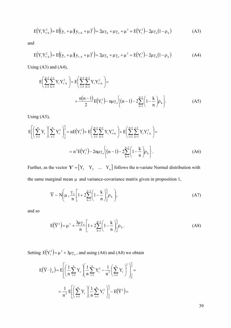
.��������.�������������
This proof requires a set of prerequisite results. Setting −= tt Yy and using (1) we have
( ) ( ) ( ) 0E2EyyE0i 0j 1jr
rktjktitrji
0i 0j
2
jktit
2
ji
2
ktt =εεεψψψ+εεψψ= ∑∑∑∑∑∞
=
∞
=
∞
+=−+−+−
∞
=
∞
=−+−+ , (A1)
and
( ) ( ) ( ) 0E2EyyE0i 0j 1jr
rktjktitrji
0i 0j
2
jktit
2
ji
2
ktt =εεεψψψ+εεψψ= ∑∑∑∑∑∞
=
∞
=
∞
+=−+−−−
∞
=
∞
=−−−− , (A2)
since ( ) 0E 3
t =ε , ( ) ( ) 0EE 2
rtr
2
t =εε=εε for rt ≠ , and ( ) 0E urt =εεε for urt ≠≠ .
Using (A1) and (A2),
Page 40
39
( ) ( )( )( ) ( ) ( )ko
3
t
3
ok
2
ktt
2
ktt 12YE2yyEYYE ρ−γ−=+γ+γ=++= ++ (A3)
and
( ) ( )( )( ) ( ) ( )ko
3
t
3
ok
2
ktt
2
ktt 12YE2yyEYYE ρ−γ−=+γ+γ=++= −− (A4)
Using (A3) and (A4),
=
=
∑∑∑∑−
=
−
=+
−
=
−
=−
1n
1t
tn
1k
2
ktt
1n
2t
1t
1k
2
ktt YYEYYE
( ) ( ) ( ) . n
k121nnYE
2
1nnk
1n
1k
o
3
t
ρ
−−−γ−−
= ∑−
=
(A5)
Using (A5),
( ) =
+
+=
∑∑∑∑∑∑−
=
−
=−
−
=
−
=+
==
1n
2t
1t
1k
2
ktt
1n
1t
tn
1k
2
ktt
3
t
n
1t
2
t
n
1t
t YYEYYEYnEYYE
( ) ( )
ρ
−−−γ−= ∑−
=k
1n
1k
o
3
t
2 n
k121nn2YEn . (A6)
Further, as the vector [ ]n21 Y...YY=′Y follows the n#variate Normal distribution with
the same marginal mean and variance#covariance matrix given in proposition 1,
ρ
−+γ
∑−
=k
1n
1k
o n
k121
n , N~Y , (A7)
and so
( ) k
1n
1k
o33 n
k121
n
3YE ρ
−+γ
+= ∑−
=
. (A8)
Setting ( ) o
33
t 3YE γ+= , and using (A6) and (A8) we obtain
( ) =
−
=γ⋅ ∑ ∑∑
= ==
n
1t
2n
1t
t2
2
t
n
1t
to Yn
1Y
n
1Y
n
1EˆYE
( )=−
= ∑∑
==
3n
1t
2
t
n
1t
t2YEY
n
1YE
n
1
Page 41
40
. n
k121n
nk
1n
1k
o
ρ
−−−γ
= ∑−
=
(A9)
Finally, Sutradhar (1994) showed that
( )
ρ
−−−γ
=γ ∑−
=k
1n
1k
oo
n
k121n
nˆE . (A10)
Hence, from (A7), (A9), and (A10) we obtain
( ) ( ) ( ) ( ) 0ˆEYEˆYEˆ,YCov ooo =γ−γ⋅=γ ,
which completes the proof.
.��������.����������� �
Using Theorem 2 of Searle (1971), which was stated in proposition 1, we have
−−−
−−−
−−−
ρρ+ρρ+ρρ
γ=⋅⋅′ ∑∑∑∑∑
−
=
−
==
−
=
−
=
1n...11
............
1...1n1
1...11n
...n
1n
0k
k
3n
0k
k
2
1k
k
2n
0k
k1
1n
0k
k3
oGΣβ .
To prove that Y and oγ̂ are not independent random variables, it is enough to show that at
least one element of the product GΣβ ⋅⋅′ is not zero. We choose the element in row 1 and
column 1 of GΣβ ⋅⋅′ which is
( ) ( )( )[ ]
ρ−+−−ρ−γ
∑ ∑−
=
−
=
1n
0k
1n
1k
kk3
o 1k23n21nn
. (A11)
The proof is completed by noting that when n is odd, the expression inside the brackets of
(A11) becomes
( ) ( ) ( )( ) 0k2n k2n k2n kkn
2
1n
1k
kn
2
1n
1k
k
2
1n
1k
<ρ−ρ−=ρ−+ρ−− −
−
=−
−
=
−
=∑∑∑ ,
while for n even this is
( ) ( ) ( )( ) 0k2n k2n k2n kkn
12
n
1k
kn
12
n
1k
k
12
n
1k
<ρ−ρ−=ρ−+ρ−− −
−
=−
−
=
−
=∑∑∑ .
Page 42
41
References
Akcay A., Biller B., Tayur S. (2011). Improved inventory targets in the presence of
limited historical data. ��������������������� ���������������, 13: 297#
309.
Akcay A., Biller B., Tayur S. (2012). A simulation#based approach to capturing
autocorrelated demand parameter uncertainty in inventory management. Proceedings
of the 2012 Winter Simulation Conference.
Ali M., Boylan J.E., Syntetos A.A. (2011). Forecast errors and inventory performance
under forecast information sharing. ������������������������������, 28(4): 830#
841.
Aviv Y. (2003). A time#series framework for supply#chain inventory management.
� ��������������, 51: 210#227.
Bayazit M., Obeysekera J.T.B., Yevjevich V. (1985). Covariance between subsample
mean and variance as related to storage variables. ���������� !"�����!, 78: 137#150.
Boylan J.E., Syntetos A.A. (2006). Accuracy and accuracy implication metrics for
intermittent demand. Foresight:�#������������������������$ ��"����������, 4:
39#42.
Charnes J.M., Marmorstein H., Zinn W. (1995). Safety stock determination with
serially correlated demand in a periodic#review inventory system. ������� ��� ����
� ��������������������!, 46: 1006#1013.
Fotopoulos S., Wang M.C., Rao S.S. (1988). Safety stock determination with
correlated demands and arbitrary lead times. %��� ��� ������� ��� � �������
�������, 35: 172#181.
Halkos G.E., Kevork I.S. (2012a). Evaluating alternative frequentist inferential
approaches for optimal order quantities in the newsvendor model under exponential
demand. MPRA Paper No. 39650.
Halkos G.E., Kevork I.S. (2012b). The classical newsvendor model under normal
demand with large coefficients of variation. MPRA Paper No. 40414.
Harvey A.C. (1993). #��� ��������"���. 2nd
Edition, Prentice Hall, An imprint of
Pearson Education Limited.
Janssen E, Strijbosch L, Brekelmans R. (2009). Assessing the effects of using demand
parameters estimates in inventory control and improving the performance using a
correction function. ���������������������&��"������%�������, 118: 34–42.
Johnson G.D., Thompson H.E. (1975). Optimality of myopic policies for certain
dependent demand processes. ���������������, 21: 1303#1307.
Page 43
42
Kang, K., Goldsman, D. (1990). The correlation between mean and variance
estimators in computer simulation. ��%�#��������, 22: 15#23.
Kevork I.S. (1990). Confidence interval methods for discrete event computer
simulation: theoretical properties and practical recommendations. Unpublished Ph.D.
thesis, University of London, London.
Kevork I.S. (2010). Estimating the optimal order quantity and the maximum expected
profit for single#period inventory decisions. ����, 38: 218–227.
Khouja M. (1999). The single#period (news#vendor) problem: literature review and
suggestions for future research. ����' 27: 537–53.
Knight K. (2000). ����������������. Taylor & Francis Ltd.
Law A.M. (2007). ����������"������"�$��!��( 4th
Edition, McGraw Hill.
Liyanage L.H., Shanthikumar J.G. (2005). A practical inventory control policy using
operational statistics. � ���������������)������( 33: 341#348.
Priestely M.B. (1981). Spectral analysis and time series. Academic Press.
Ray W.D. (1982). ARIMA forecasting models in inventory control. ������� ��� ����
� ��������������������!, 33: 567#574.
Ritchken P.H., Sankar R. (1984). The effect of estimation risk in establishing safety
stock levels in an inventory model. #������������������ ��������������������!,
35: 1091–1099.
Searle S.R. (1971). )������"���. John Wiley & Sons, new York, NY.
Silver E.A., Pyke D.F., Peterson R. (1998). ��������!���������� �"� ��"������
�������"�����"����( 3rd
Edition, New York, John Wiley and Sons.
Strijbosch L.W.G., Syntetos A.A., Boylan J.E., Janssen E. (2011). On the interaction
between forecasting and stock control: The case of non#stationary demand.
���������������������&��"������%�������, 133: 470#480.
Sutradhar B.C. (1994). Moments of the sampled autocovariances and autocorrelations
for a general Gaussian process. ��*�!+�#�����"�������������������, 56(B): 272#
285.
Syntetos A.A., Nikolopoulos K., Boylan J.E. (2010). Judging the judges through
accuracy#implication metrics: The case of inventory forecasting. �����������
�������������������, 26: 134–143.
Syntetos A.A., Boylan J.E. (2008). Demand forecasting adjustments for service#level
achievement. ��$����������������������������, 19: 175#192.
Page 44
43
Urban T.L. (2000). Reorder level determination with serially#correlated demand.
��������������� ��������������������!, 51: 762#768.
Urban T.L. (2005). A periodic#review model with serially#correlated, inventory#level#
dependent demand. ���������������������&��"������%�������, 95: 287#295.
Zhang X. (2007). Inventory control under temporal demand heteroskedasticity.
%��� �������������� ��������������, 182: 127#144.
Zinn W., Marmorstein H., Charnes J. (1992). The effect of autocorrelated demand on
customer service. ����������,�������)������, 13: 173#192.