Tree Physiology 9, 147-160 0 1991 Heron Publishing-Victoria, Canada FOREST-BGC, A general model of forest ecosystem processes for regional applications. II. Dynamic carbon allocation and nitrogen budgets’ STEVEN W. RUNNING2 and STITH T. GOWER3 ’ School of Forestry, University of Montana, Missoula, MT 59812, USA 3 Department of Forestry, University of Wisconsin, Madison, WI 53706, USA Summary A new version of the ecosystem process model FOREST-BGC is presented that uses stand water and nitrogen limitations to alter the leaf/root/stem carbon allocation fraction dynamically at each annual iteration. Water deficit is defined by integrating a daily soil water deficit fraction annually. Current nitrogen limitation is defined relative to a hypothetical optimum foliar N pool, computed as maximum leaf area index multiplied by maximum leaf nitrogen concentration. Decreasing availability of water or nitrogen, or both, reduces the leaf/root carbon partitioning ratio. Leaf and root N concentrations, and maximum leaf photosynthetic capacity are also redefined annually as functions of nitrogen availability. Test simulations for hypothetical coniferous forests were performed for Madison, WI and Missoula, MT, and showed simulated leaf area index ranging from 4.5 for a control stand at Missoula, to 11 for a fertilized stand at Madison, with Year 50 stem carbon biomasses of 31 and 128 Mg ha-‘, respectively. Total nitrogen incorporated into new tissue ranged from 34 kg ha-’ yea-’ for the unfertilized Missoula stand, to 109 kg ha-’ year-t for the fertilized Madison stand. The model successfully showed dynamic annual carbon partitioning controlled by water and nitrogen limitations. Introduction A primary limitation to our ability to complete a carbon balance of forests and to model forest growth from “first principles” of tree physiology has been a poor understanding of the partitioning of photosynthetic production to permanent tissue (Landsberg 1986). Early studies showed that as much as 60% of annual net photo- synthate was invested in root production, but, because of high annual root mortality and turnover, relatively little permanent root biomass remained (Kinerson et al. 1977, Santantonio et al. 1977). Later studies illustrated substantial variability in above- ground/helowground carbon partitioning related to the availability of water and nutrients (Keyes and Grier 1981, Grier et al. 1981, Linder and Troeng 1981, Nadelhoffer et al. 1985). Attempts to formalize and model abovegroundl belowground carbon partitioning have borrowed from economic theory (Bloom et al. 1985), optimization logic (Hof et al. 1990), and theoretical modeling (Agren and Ingestad 1987). In the first generation of forest carbon models exhibiting variable carbon partition- ing, aboveground/helowground allocation or leaf/root growth was controlled mainly by external parameters (McMurtrie and Wolf 1983, Oikawa 1985, Mohren 1987, ’ The FOREST-BGC model program and source code are available from the senior author.
Transcript
Tree Physiology 9, 147-160 0 1991 Heron Publishing-Victoria, Canada
FOREST-BGC, A general model of forest ecosystem processes for regional applications. II. Dynamic carbon allocation and nitrogen budgets’
STEVEN W. RUNNING2 and STITH T. GOWER3 ’ School of Forestry, University of Montana, Missoula, MT 59812, USA 3 Department of Forestry, University of Wisconsin, Madison, WI 53706, USA
Summary
A new version of the ecosystem process model FOREST-BGC is presented that uses stand water and nitrogen limitations to alter the leaf/root/stem carbon allocation fraction dynamically at each annual iteration. Water deficit is defined by integrating a daily soil water deficit fraction annually. Current nitrogen limitation is defined relative to a hypothetical optimum foliar N pool, computed as maximum leaf area index multiplied by maximum leaf nitrogen concentration. Decreasing availability of water or nitrogen, or both, reduces the leaf/root carbon partitioning ratio. Leaf and root N concentrations, and maximum leaf photosynthetic capacity are also redefined annually as functions of nitrogen availability. Test simulations for hypothetical coniferous forests were performed for Madison, WI and Missoula, MT, and showed simulated leaf area index ranging from 4.5 for a control stand at Missoula, to 11 for a fertilized stand at Madison, with Year 50 stem carbon biomasses of 31 and 128 Mg ha-‘, respectively. Total nitrogen incorporated into new tissue ranged from 34 kg ha-’ yea-’ for the unfertilized Missoula stand, to 109 kg ha-’ year-t for the fertilized Madison stand. The model successfully showed dynamic annual carbon partitioning controlled by water and nitrogen limitations.
Introduction
A primary limitation to our ability to complete a carbon balance of forests and to model forest growth from “first principles” of tree physiology has been a poor understanding of the partitioning of photosynthetic production to permanent tissue (Landsberg 1986). Early studies showed that as much as 60% of annual net photo- synthate was invested in root production, but, because of high annual root mortality and turnover, relatively little permanent root biomass remained (Kinerson et al. 1977, Santantonio et al. 1977). Later studies illustrated substantial variability in above- ground/helowground carbon partitioning related to the availability of water and nutrients (Keyes and Grier 1981, Grier et al. 1981, Linder and Troeng 1981, Nadelhoffer et al. 1985). Attempts to formalize and model abovegroundl belowground carbon partitioning have borrowed from economic theory (Bloom et al. 1985), optimization logic (Hof et al. 1990), and theoretical modeling (Agren and Ingestad 1987).
In the first generation of forest carbon models exhibiting variable carbon partition- ing, aboveground/helowground allocation or leaf/root growth was controlled mainly by external parameters (McMurtrie and Wolf 1983, Oikawa 1985, Mohren 1987,
’ The FOREST-BGC model program and source code are available from the senior author.
148 RUNNING AND GOWER
Running and Coughlan 1988). We have now developed a model that allows dynamic changes in leaf/root carbon allocation, controlled annually by carbon, nitrogen and water availability. In this paper we present the theory and algorithms for this carbon partitioning, the optimization logic used to determine at each yearly timestep which of the three controlling factors will limit partitioning, and test runs under control and fertilized conditions for two climates.
The FOREST-BGC model
A compartment flow diagram for the FOREST-BGC model is shown in Figure 1 (see also Running and Coughlan 1988). A complete description of the daily half of the model has been published (Running and Coughlan 1988, Hunt et al. 1991). Changes made to the original version of the model include definition of all 20 state variables, and many new constant parameters have been defined for the carbon and nitrogen calculations presented here (Table 1). In essence, the entire yearly half of the old model with its “static” carbon budget has been replaced with dynamic and interacting carbon and nitrogen budgets.
In addition, it is now possible to direct the simulation to loop to the “yearly” half at any timestep, e.g., weekly, so that within-year activity of carbon and nitrogen can be simulated. It is also possible to change the value of a constant parameter within a seasonal simulation, or within the life cycle of a stand, using MS-DOS textfiles. There is also a version of the model with hourly, rather than daily hydrologic and canopy process simulations.
Model logic
The FOREST-BGC model structure, as presented in Running and Coughlan (1988)
Figure 1. A compartment flow diagram of the FOREST-BGC simulation model. This diagram illustrates the compartments of carbon, water and nitrogen, the critical mass flow linkages, and the mixed daily/annual time resolution (from Running and Coughlan 1988, with permission).
A GENERAL MODEL OF FOREST ECOSYSTEM PROCESSES 149
Table 1. Initial state variables and parameters for model runs, using the Madison site fertilized with 100 kg N at Year 20 as an example.
Specific leaf area m* kg-’ Canopy light extinction coefficient Soil water capacity Water interception coefficient Snowmelt coefficient Latitude 1 - surface albedo
m3 ha-’ m L*-’ day-’ m “C-’ day-’ degree
Minimum water potential in spring Radiation reducing leaf conductance threshold Maximum canopy average leaf conductance Leaf water potential at stomata1 closure Slope of absolute humidity reduction Photosynthesis light compensation point Photosynthesis maximum Maximum leaf conductance (CO2) Minimum temperature for photosynthesis Maximum temperature for photosynthesis Leaf respiration coefficient Stem respiration coefficient Root respiration coefficient Temperature effect on mesophyll condition coefficient Decomposition temperature optimum Q’a = 2.3 for exponential respiration surface Maximum canopy average leaf nitrogen concentration Minimum canopy average leaf nitrogen concentration Leaf nitrogen retranslocation fraction Soil/litter decomposition rate fraction Nitrogen/carbon decomposition release fraction
MPa kJ m-2 day-’ ms -1
MPa m S- Habs -I
kJ mm2 k.I me2 day-’ ms-’ “C “C kg kg-’ “C-’ day-’ kg kg-’ “C-’ day-’ kg kg-’ “C-’ day-’ “C “C “C kg N kg-’ C kg N kg’ C fraction year-’ fraction year-’
m3 ha-’ m3 ha-’ m3 ha-’ m3 ha-’ m3 ha-’ kg ha-’ kg ha-’ kg ha-’ kg ha-’ kg ha-’ kg ha-’ kg ha-’ kg ha-’ kg ha-’ kg ha-’ kg ha-’ kg ha-’ kg ha-’ kg ha-’ kg ha-’
150 RUNNING AND GOWER
Table 1. Cont’d.
Initial value Description Unit
12 Maximum leaf area index, all sides 4 Leaf turnover age 25 Leaf lignin fraction 1 Soil water leaf/root allocation factor 1 Nitrogen availability leaf/root allocation factor 20 Mobile N retention time 5 Atmospheric N deposition 0 Biological N fixation 0.02 Stem turnover coefficient 0.8 Root turnover coefficient 0.35 Leaf growth respiration 0.3 Stem growth respiration 0.35 Root growth respiration
m2 m-* years %
years kg ha-’ year-’ kg ha-’ year-’ fraction year-’ fraction year-’ kg kg-’ C kg kg-’ C kg kg-’ C
defined leaf, stem, and root carbon compartments that received annual carbon allocations from accumulated net photosynthesis (GL). Maintenance respiration of leaf, stem and root tissues was subtracted daily, controlled by temperature, leaving all of the residual assimilate at the end of the year available for growth. The fraction of net photosynthate allocated to these three sinks was specified by externally defined parameters (see Table 3 in Running and Coughlan 1988) as 0.25,0.35 and 0.40 (= 100% of net photosynthate available) for leaf, stem and root carbon alloca- tion, respectively. In both model versions, after carbon has been allocated to the leaf, stem and root compartments, growth respiration for leaf, stem and root tissues is subtracted, and the remaining carbon “deposited” in the compartments as new growth. The growth respiration fractions subtracted are derived from the biochemical energetics logic of Penning De Vries et al. (1974).
Limitations to leaf growth
The FOREST-BGC model emphasizes leaf area index (L*) as a key structural attribute with substantial control over ecosystem process rates. This version of the FOREST-BGC model begins the optimization process by calculating the L* that could be produced if carbon (net photosynthate), water or nitrogen alone were limiting. Carbon available for leaf growth when leaf growth is limited only by the supply of photosynthate (C,, kg C ha-’ year-‘) is determined by annual net photosynthate (GL, kg C ha-’ year-‘) and the (dimensionless) leaf/root partitioning ratio (RR&:
CLC = GL RLIR (1)
Because the final leaf/root carbon partitioning cannot be known until the end of the computation, a preliminary leaf/root partitioning ratio provides an initial estimate of the proportion of net photosynthate available for leaf growth.
A GENERAL MODEL OF FOREST ECOSYSTEM PROCESSES 151
The value of CLc places an upper limit on the carbon available for leaf growth, which prevents the model from producing excessive leaf area when water and nitrogen are in adequate supply, and allows a controlled simulation of development from seedling to sapling beginning from a small L*.
Leaf growth may be modified by leaf water status, which is determined by the ratio of the highest simulated predawn leaf water stress, YL, to a defined maximum leaf water stress, Y,,,, usually around 1 J-2.0 MPa. This modification allows the model to produce more leaf area the following year if the water stress Y,,, (which equals the water potential with the sign reversed) is not reached, but provides a feedback control lowering L* if ‘Pm,, is exceeded.
CLY=CLCWmax/YL) (2)
where CLy, kg C ha-’ year-‘, . 1s carbon available for leaf growth when leaf growth is limited by water stress.
Leaf growth may also be modified by nitrogen availability, in which case the current available N pool, divided by the leaf N concentration defines the carbon available for leaf growth (CLN, kg C ha-’ year-‘):
CLN=CLC (NavadJ'JL) (3)
where NL is current leaf nitrogen concentration, kg N kg-’ C and Navait is available nitrogen, kg ha-‘. Nitrogen availability is defined using an approach similar to the N productivity concept of Agren (1983) in which maximum needle biomass is con- trolled by available N (see Equation 8).
The model then takes the smallest of C ~c, CLY and CLN as the carbon actually allocated to leaf growth (CL) and computes L* as:
L” = CL SLA, (4)
where SLA is specific leaf area (m* kg-’ C), an externally determined model parameter.
Leaflroot partitioning ratio
The final leaf/root carbon partitioning ratio (RLE) ranges between 0.5 (33% to leaves, 67% to roots) and 0.1 (9% to leaves, 91% to roots) (cf. Cannel1 1985). The final L/R ratio is defined by summing a soil water index (Zsw) and a nitrogen availability index (IN). For the soil water index, the logic of Grier and Running (1977) and Nemani and Running (1989) relating site water balance to a “carrying capacity” of L* is repre- sented, where the water balance is defined as the average soil water deficit (fraction of field capacity) computed by the daily hydrologic balance in FOREST-BGC. Equation 12 uses this same soil water index as part of the decomposition calculations.
Once RL~ has been calculated, and the limit on carbon available for leaf growth defined by Equations 1-3, the model allocates the absolute quantity of carbon to
152 RUNNING AND GOWER
leaves (CL) and roots (CR).
CL=GLRLIR
CR = CL 1IRm
CST=GL-CL-CR (7)
Stem allocation, CST, is not explicitly defined, but is generated as a residual after leaf and root growth have been satisfied.
This procedure allocates carbon according to the following priorities: (1) mainte- nance respiration, (2) growth respiration, (3) leaf growth, (4) root growth, (5) stem growth. Although it is mathematically possible for leaf and root growth to consume all available annual photosynthate, leaving nothing for stem growth, it is biologically impossible for stem growth to be zero because leaf growth is controlled by water or nitrogen so that all available carbon is not consumed. No reproductive carbon, starch storage pool or defensive chemical production is currently defined.
For every unit of leaf growth an appropriate quantity of root biomass will be required to provide the necessary water and nutrients. Specific root functions, such as hydraulic conductivity and water and nutrient uptake are not simulated.
Nitrogen budget
The nitrogen budget is most sensitive to the compartment sizes and decomposition rates of N in the litter and soil. These pools are conceptually equivalent to the active and slow soil organic matter and N pools of the Century model (Par-ton et al. 1987). The amount of leaf litter incorporated in the soil pool is proportional to the leaf lignin concentration, the remainder goes to the litter compartment. For the present simula- tions, 25% of leaf litter was directed to the soil carbon and nitrogen pools, and 75% to the litter pools of carbon and nitrogen.
Input to the litter and soil pools is from annual leaf fall and root mortality. Leaf turnover rate (or leaf longevity) has a marked effect on the rate of carbon and nutrient cycling, but no simple relationship exists between leaf longevity and climate or fertility (Vogt et al. 1986). However, trends detected by Gower et al. (unpublished observations) suggest that increased fertility is positively correlated with leaf longev- ity of natural, unfertilized conifer stands. Leaf turnover age is one of the most sensitive parameters in the model because it connects the annual dynamics of carbon and nitrogen turnover. Stem turnover is effectively a stand mortality rate, because large biomass decomposition is not defined.
A major component of the nitrogen budget is the concentration of N in leaf and root tissues. A general N availability index is first defined by:
IN = Navad(W*max NL,~~J/SLA)
where IN is the fractional N availability index, {O-l ) , I,*,,,, is the maximum defined
A GENERAL MODEL OF FOREST ECOSYSTEM PROCESSES 153
site L*, and NL,max is the maximum defined leaf N concentration, kg N kg-’ C. The N available for canopy growth is defined as:
NC = (Navail R~/~)l(L*max N~,max) (9)
where NC is the fractional index of N available for canopy growth, (O-l 1. Current leaf nitrogen concentration, NL, is defined by the equation:
NL = (N~,max - NL,min) NC + NL,min (10)
where NL is leaf nitrogen concentration, kg N kg-’ C, and Nr,min is the minimum defined leaf N concentration, kg N kg-’ C.
Equation 10 calculates an NL range equivalent to 0.6-2.0% N per leaf dry weight, which is appropriate for conifers. For deciduous trees or other plant types NL and NL,~,, can easily be redefined to give a new NL range. Root nitrogen concentration, NR, is set at 50% of the calculated NL. Representation of the nitrogen cycle depends on canopy nitrogen and avoids reference to belowground pools or processes in an attempt to simplify complex physiological and biogeochemical processes. This allows regional applications and canopy-oriented, remote sensing definitions of key ecosystem variables (Wessman et al. 1988).
The canopy turnover functions produce a balancing point for the interaction of the carbon and nitrogen cycles. A fertile site will have a high NL, which then requires more N per unit of leaf (and root) mass grown, or less L* per unit N. However, NL positively controls maximum canopy photosynthesis rate, as suggested by Field et al. (1983), producing more fixed carbon.
Leaf retranslocation before litterfall is also important, and is defined by a leaf nitrogen retranslocation fraction, currently 50% of original NL (Prescott et al. 1989). Retranslocation of root nitrogen is thought to be zero (Nambiar 1987). However, fine root decomposition and reabsorption of that nitrogen is probably rapid so that, for an annual timestep, the model returns all NR from root turnover to the available N pool.
The decomposition rates of the soil and litter pools are calculated as functions of the integrated daily average water fraction and a daily temperature degree day summation, both provided from the daily half of the model:
Ts = (=~/365)~0,, (11)
where TS is the fractional expression {O-l ) of annual average soil temperature at 20 cm, C is the summation of daily soil temperatures, T, and To,, is the optimum decomposition temperature “C.
ws =C(WD)/F,,@~~ (12)
where WS is the fractional expression {O-l ) of annual average soil water content, WD is daily soil water content, m3 ha-‘, and Fcap is field soil water capacity, m3 ha-‘.
154 RUNNING AND GOWER
The basic decomposition rate is then defined as the sum of these two fractions:
km = (Ts + wd4.0 (13)
where kLTc is the decomposition rate for leaf/root litter carbon, year-‘, and 4.0 is a scaling factor that allows a maximum decomposition rate of 0.5, (i.e., a 2-year turnover time).
This logic is functionally similar to the Actual ET (Evapotranspiration) control decomposition model of Meetenmeyer (197Q except that we model evapotranspi- ration explicitly in generating the soil water content, and we separate temperature and water driving variables.
Decomposition mobilizes nitrogen at a fraction (currently 50%) of the rate that carbon is released to simulate the decrease in C/N ratio found as microbial popula- tions immobilize nitrogen:
kriv =NLT UkLTc (14)
where kLTN is the litter N mineralization rate, kg year-‘, NLT is the litter N compart- ment, kg ha-‘, and a is the fraction of N release relative to C release.
The soil decomposition pools for carbon and nitrogen decay at a fractional rate of the litter pools, currently 3%.
kc = cs FSIL kLTc (15)
km = Ns FS,L k-rc (16)
where ksc is carbon release from the soil C pool, kg ha-’ year-‘, Cs is the soil C compartment, kg ha-‘, Ns is the soil N compartment, kg ha-‘, and Fsk is the fractional constant of soil/litter decomposition rates.
Annual turnover rates ranging from 15% at Fairbanks, AK, to 87% at Jacksonville, FL, have been calculated for fixed lignin concentrations of 15% (Running and Coughlan 1988). The soil nitrogen pool also releases a fraction of the N pool annually to external losses, such as leaching or volatilization. This is the only point of N removal from the system.
Test simulations
The model structure was tested by making 50-year simulations for forest stands in Madison WI, representing a cool, wet climate, and in Missoula, MT, representing a cool, dry climate. A single-year climate tile, 1984, was repeated for the 50 years. Control runs were made with an annual N input of 5 kg ha-’ at each site, and a fertilization simulation of 25 kg ha-’ year- ’ N input was also run. Additionally, a simulation for Madison was run with a one-time 100 kg ha-’ fertilization at Year 20. On Day 1 of the simulation, the snowpack was initialized at 12.1 cm and soil water
A GENERAL MODEL OF FOREST ECOSYSTEM PROCESSES 155
at 23.3 cm. Leaf carbon was initialized for all runs at 1.2 Mg C ha-‘, equivalent to a total L* = 3, and stem carbon at 10 Mg ha-‘. The active litter compartment was defined as 3 Mg ha-’ for C and 300 kg ha-’ for N, and the soil compartments were 40 Mg ha-’ and 2000 kg ha-’ N. For the Missoula simulations, only the snowpack, soil water content and latitude were defined differently.
Results
Carbon budget
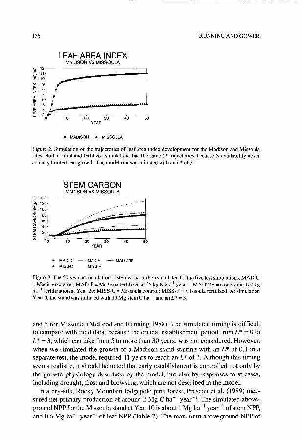
The 50-year simulation results for the fertilized Madison site and the control Mis- soula site are given in Table 2, and the L* and stem biomass trends are shown in Figures 2 and 3. Beginning with a “sapling” of L* = 3, L* equilibrates to about 10 for the Madison stand and 4.5 for the Missoula stand by around Year 10. At each site, both control and fertilized stands produce the same L*, because nitrogen availability never controlled leaf area development, which may be a model error. These values of L* are close to the measured values of 13 for Madison (Gower and Norman 1990)
Table 2. Simulation results for two 50.year runs.
Year T’ GPP’ RN’ RG’ CL*
Missoula control, 5 kg N ha-’ year-’ 1 24.7 4.5 1.3 1.5
’ Transpiration, cm H20 year-‘. 2 Mg C ha-’ year-‘. 3 kg N ha-’ year-‘.
156
LEAF AREA INDEX MADISON VS MISSOULA
RUNNING AND GOWER
9 5 9 4 !Y 3
0 10 20 30 40 50 YEAR
-- MADISON * MISSOULA
Figure 2. Simulation of the trajectories of leaf area index development for the Madison and Missoula sites. Both control and fertilized simulations had the same L* trajectories, because N availability never actually limited leaf growth. The model run was initiated with an L* of 3.
STEM CARBON MADISON VS MISSOULA
= MAD-C - MAD-F + MAD-POF A MISS-C MISS-F
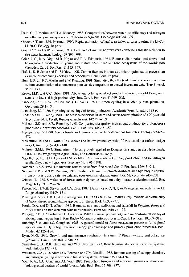
Figure 3. The 50.year accumulation of stemwood carbon simulated for the five test simulations, MAD-C = Madison control; MAD-F = Madison fertilized at 25 kg N ha-’ year-‘, MAD20F = a one-time 100 kg ha-’ fertilization at Year 20; MISS-C = Missoula control; MISS-F = Missoula fertilized. At simulation Year 0, the stand was initiated with 10 Mg stem C ha-’ and an L* = 3.
and 5 for Missoula (McLeod and Running 1988). The simulated timing is difficult to compare with field data, because the crucial establishment period from L* = 0 to L* = 3, which can take from 5 to more than 30 years, was not considered. However, when we simulated the growth of a Madison stand starting with an L* of 0.1 in a separate test, the model required 11 years to reach an L* of 3. Although this timing seems realistic, it should be noted that early establishment is controlled not only by the growth physiology described by the model, but also by responses to stresses, including drought, frost and browsing, which are not described in the model.
In a dry-site, Rocky Mountain lodgepole pine forest, Prescott et al. (1989) mea- sured net primary production of around 2 Mg C ha-’ year-‘. The simulated above- ground NPP for the Missoula stand at Year 10 is about 1 Mg ha-’ year-’ of stem NPP, and 0.6 Mg ha-’ year-’ of leaf NPP (Table 2). The maximum aboveground NPP of
A GENERAL MODEL OF FOREST ECOSYSTEM PROCESSES 157
the Madison simulation, again around Year 10, after L* had been optimized, but before major respiration loading occurred, was about 4.2 Mg C ha-’ year-‘, and for the fertilized simulation it was about 5.4 Mg C ha-’ year-‘.
The stem carbon trends show two particularly interesting results. First, in a dry environment like that of the Missoula stand, fertilization increased stem biomass at 50 years by 45% from 31 to 45 Mg C ha-‘, whereas in the Madison stand, stem biomass increased by 58% from 81 to 128 Mg C ha-‘, which may be optimistic. Second, the one-time fertilization of the Madison site at Year 20 resulted in a measurable, but only temporary, improvement in stem primary production and biomass development (Figures 3 and 4).
At all sites, stem biomass was still accumulating at Year 50. The Missoula control stand showed a simulated NPP of about 0.8 Mg ha-’ year-‘, but stem primary production was only 0.03 Mg ha-’ year- ‘, because of maintenance respiration. Although 4.7 Mg ha-’ of gross primary production remained after respiration losses and leaf and root replacement, the amount available for stem growth was small. Additional work on quantifying absolute magnitudes of maintenance respiration (Ryan 1990) is required. The simulated stem carbon mass at Year 50 at Missoula was 3 1 Mg ha-’ compared to an aboveground biomass at age 90 of about 50 Mg C ha-’ as measured by Prescott et al. (1989) for a lodgepole pine stand in Alberta. Year 50 stem carbon was 81 Mg ha-’ for the Madison control simulation. Field data from Minnesota for 40-year-old Pinus resinosa stands show aboveground biomass of 76-94 Mg C ha-’ (Perala and Alban 1982). At Year 50, the Madison fertilizer simulation still had nearly 11 Mg ha-’ GPP and a net stem NPP of almost 1 Mg ha-‘.
Despite the much higher litter production rate on the fertilized Madison site compared with the Missoula site, the Missoula site at Year 50 had the greatest active litter carbon pool, 22 Mg ha-’ compared to 19 Mg ha-‘, reflecting the more rapid decomposition at Madison. The simulated litter turnover rate was 10% year-’ at Missoula, and 19% year-’ at Madison, where frequent summer rainfall keeps litter wet. The control simulations show leaf nitrogen concentrations at Year 50 of 0.026
LEAF/STEM/ROOT C ALLOCATION FERTILIZED YR 20, MADISON
YEAR
m STEM ROOT m LEAF
Figure 4. An illustration of the variable carbon partitioning exhibited by the model during a 30.year period for the Madison-Year 20 fertilized simulation. Note the change in allocation after the one-time Year 20 fertilization.
158 RUNNING AND GOWER
kg N kg-’ C (1.2% DW). Simulations of the fertilized sites had 0.044 kg N kg-’ C (2.0% DW), even after beginning the simulations at a conservative 0.015 kg N kg-’ C (0.7% DW). Total canopy nitrogen ranged from 53 kg ha-’ in the Missoula control to 194 kg ha-’ in the Madison fertilized stand; the active litter N pools ranged from 136 kg ha-’ to 253 kg ha-’ for the Missoula and Madison stands, respectively (Table 2).
Table 3 shows the annual inputs of N to the available pool at Year 30, near the midpoint of the simulation when the N budgets and C partitioning had stabilized. The modeled sources of input to the available N pool are retranslocation from root and leaf compartments before litterfall, N mineralization from the litter and soil compart- ments, and external inputs from atmospheric or fertilization sources. The model does not differentiate between root N retranslocation and root litter N turnover, and so calculates fine root litter N decomposition as 100% year-‘, returning all root turnover N back to the tree. This logic approximates some poorly understood physiology concerning the sources, magnitudes and timing of available N in the root-litter-soil complex. We suggest this treatment is reasonable for describing nitrogen processes at annual timesteps representing a steady-state system. However, the decomposition and root retranslocation results combined may better represent the annual system N mineralization measured in field studies.
The higher L* at Madison resulting in more leaf litter, coupled with higher decomposition rates results in the production of more available N at Madison than at Missoula. Even the fertilization treatment at Missoula only increased N availability from 34 to 41 kg ha-’ year-’ total N, because of overwhelming water limitations. In the model dynamics, carbon is required to retain and cycle nitrogen, and the weak carbon budget at Missoula simply cannot cycle much nitrogen, even when nitrogen is made available through fertilization.
Dynamic C partitioning
The test simulations showed that stem C allocation in Year 30 ranged from 0.26 for the Missoula control stand to 0.50 for the Madison fertilized stand, with little change
Table 3. Nitrogen cycle components at Year 30, given identical initial N pools at Year 0.
’ All units are kg N ha-’ year-‘. * Control treatment received 5 kg N ha-’ year-’ , fertilized treatment received 25 kg N ha-’ year-‘. 3 See text for explanation of root N retranslocation logic.
A GENERAL MODEL OF FOREST ECOSYSTEM PROCESSES 159
in later years (Table 4). Leaf carbon allocation, as a fraction of total photosynthate, remained essentially constant at 14-16%, although those fractions operated on net available photosynthate ranging from 4.8 to 11.7 Mg C ha-’ year-‘. Consequently, the more fertile sites had higher absolute carbon allocation to leaves, because of higher available photosynthate and higher L* than the poor sites. Because stem carbon allocation is treated in the model as a residual after leaf and root carbon needs are met, increased demand for root carbon was directly reflected in reduced stem carbon. These dynamics compare well with the logic and synthesized data presented by Cannel1 (1989).
Table 4. Carbon allocation fractions at Year 30 of the 50-year simulations.
Total GPP’ Leaf Stem Root
Madison Control 10.2 0.16 0.34 0.50 Fertilized 11.7 0.14 0.50 0.35 Fertilized at Year 20 10.6 0.16 0.39 0.46
Changes in partitioning dynamics with life cycle for the Madison simulation with fertilization at Year 20 are illustrated in Figure 4. For the first few years, root carbon allocation is nearly 70%, and the remainder is leaf allocation. Stem allocation as abstracted in this model stabilizes around Year 7. The single 100 kg N fertilization at Year 20 resulted in an instantaneous decline in root allocation and an increase in stem allocation. However, after about 5 years, the added N has cycled through the canopy, has been deposited as litter or soil N, and its influence has declined as it has been slowly mineralized.
Acknowledgments
In developing FOREST-BGC we have had helpful discussions with Drs. Richard Waring, E. Raymond Hunt, Jr., Mike Ryan, Kate Lajtha, and Henry Gholz. Funding for this work has been provided by NASA grant NAGW-952, NASA Joint Research Interchange #NCA2-252 with the Ames Research Center, NSF grant #NSR-8919646, and M&tire-Stennis Funding to the University of Montana.
References Agren, G.I. 1983. Nitrogen productivity of some conifers. Can. J. For. Res. 13:494-500. Agren, G.I. and T. Ingestad. 1987. Root:shoot ratio as a balance between nitrogen productivity and
photosynthesis. Plant, Cell Environ. 10:579-586. Bloom, A.J., ES. Chapin and H.A. Mooney. 1985. Resource limitation in plants-an economic analogy.
Ann. Rev. Ecol. System. 16:363-392. Cannell, M.G.R. 1985. Dry matter partitioning of tree crops. In Attributes of Trees as Crop Plants. Eds.,
M.G.R. Cannel1 and J.E. Jackson. Inst. of Terrestrial Ecology, Midlothian Scotland, pp 160-193. Cannell, M.G.R. 1989. Physiological basis of wood production: a review. Stand. J. For. Res. 4:459-490.
160 RUNNING AND GOWER
Field, C., J. Merino and H.A. Mooney. 1983. Compromises between water use efficiency and nitrogen use efficiency in five species of California evergreens. Oecologia 60:384-389.
Gower, S.T. and J.M. Norman. 1990. Rapid estimation of leaf area index in forests using the Li-Cor LI-2000. Ecology. In press.
Grier, C.C. and S.W. Running. 1977. Leaf area of mature northwestern coniferous forests: Relation to site water balance. Ecology 58893-899.
Grier, C.C., K.A. Vogt, M.R. Keyes and R.L. Edmonds. 1981. Biomass distribution and above- and belowground production in young and mature Abies amabilis zone ecosystems of the Washington Cascades. Can. J. For. Res. 11:155-167.
Hof, J., D. Rideout and D. Binkley. 1990. Carbon fixation in trees as a micro optimization process: an example of combining ecology and economics. Ecol. Econ. In press.
Hunt, E.R. Jr., EC. Martin and S.W. Running. 1991. Simulating the effects of climatic variation on stem carbon accumulation of a ponderosa pine stand: comparison to annual increment data. Tree Physiol. 9:161-171
Keyes, M.R. and C.C. Grier. 1981. Above and belowground net production in 40 year old Douglas-fir stands on low and high productivity sites. Can. J. For. Res. 11:599-605.
Kinerson, R.S., C.W. Ralston and C.G. Wells. 1977. Carbon cycling in a loblolly pine plantation. Oecologia 29: I-10.
Landsberg, J.J. 1986. Physiological ecology of forest production. Academic Press, London, 198 p. Linder, S and E. Troeng. 1981. The seasonal variation in stem and coarse root respiration of a 20-year-old
Scats pine. Mitt. Forstl. Bundesversuchsanst. 142: 125-139. McLeod, S.D. and S.W. Running. 1988. Comparing site quality indices and productivity in Ponderosa
pine stands in western Montana. Can. J. For. Res. 18:346-352. Meetenmeyer, V. 1978. Macroclimate and lignin control of litter decomposition rates. Ecology 59:465-
472. McMurtrie, R. and L. Wolf. 1983. Above and below ground growth of forest stands: a carbon budget
model. AM. Bot. 52:437-448. Mohren, G.M.J. 1987. Simulation of forest growth, applied to Douglas-fir stands in the Netherlands.
Ph.D. Diss., Wageningen Agric. Univ., The Netherlands, 184 p. Nadelhoffer, K.J., J.D. Aber and J.M. Melillo. 1985. Fine roots, net primary production, and soil nitrogen
availability: a new hypothesis. Ecology 66: 1370-1390. Nambiar, E.K.S. 1987. Do nutrients retranslocate from fine roots? Can. J. For. Res. 17:913-918. Nemani, R.R. and S.W. Running. 1989. Testing a theoretical climate-soil-leaf area hydrologic equilib-
rium of forests using satellite data and ecosystem simulation. Agric. For. Meteorol. 44:245-260. Oikawa, T. 1985. Simulation of forest carbon dynamics based on a dry-matter production model. Bot.
Mag. Tokyo 98:225-238. Parton, W.J., J.W.B. Stewart and C.V. Cole. 1987. Dynamics of C, N, P, and S in grassland soils: a model.
Biogeochemistry 5:109-131. Penning de Vries, F.W.T., A. Brunsting and H.H. van Laar. 1974. Products, requirements and efficiency
of biosynthesis; a quantitative approach. J. Theor. Biol. 45:339-377. Perala, D.A. and D.H. Alban. 1982. Biomass, nutrient distribution and litterfall in Populus, Pinus and
Picea stands on two different soils in Minnesota. Plant Soil 64:177-192. Prescott, C.E., J.P Corbin and D. Parkinson. 1989. Biomass, productivity, and nutrient-use efficiency of
aboveground vegetation in four Rocky Mountain coniferous forests. Can. J. For. Res. 19:309-317. Running, S.W. and J.C. Coughlan. 1988. A general model of forest ecosystem processes for regional
applications. I. Hydrologic balance, canopy gas exchange and primary production processes. Ecol. Model. 42:125-154.
Ryan, M.G. 1990. Growth and maintenance respiration in stems of Pinus contorta and Picea en- gelmannii. Can. J. For. Res. 20:48-57.
Santantonio, D., R.K. Hermam and W.S. Overton. 1977. Root biomass studies in forest ecosystems. Pedobiologia 17: l-3 1.
Wessman, C.A., J.D. Aber, D.L. Peterson and J.M. Melillo. 1988. Remote sensing of canopy chemistry and nitrogen cycling in temperate forest ecosystems. Nature 335: 154-1.56.
Vogt, K.A., C.C. Grier and D.J. Vogt. 1986. Production, turnover and nutrient dynamics of above- and belowground detritus of world forests. Adv. Ecol. Res. 15:303-377.