44
Foundations of Science-based Target Setting Version 1.0 April 2019

Foundations of Science-based Target Setting
Version 1.0
April 2019

Foundations of Science-based Target Setting 1.0 2
Table of Contents
1. Introduction ...............................................................................................................................4
1.1 Outline ........................................................................................................................4
2. Background ................................................................................................................................6
2.1 Target-setting methods ................................................................................................6
GHG budgets ......................................................................................................................................... 7
Emissions scenarios ............................................................................................................................... 7
Allocation approach .............................................................................................................................. 8
Constructing SBTi methods ................................................................................................................... 8
Box 1. Understanding scenarios ..............................................................................................9
Box 2. Determining useful GHG budgets ............................................................................... 11
3. Methods and scenarios the SBTi currently endorses .................................................................. 13
3.1 Absolute Contraction ................................................................................................. 13
Determining a scenario envelope ....................................................................................................... 13
Results ................................................................................................................................................. 21
3.2 Sectoral Decarbonization Approach ............................................................................ 24
Overview ............................................................................................................................................. 24
ETP scenario modelling ....................................................................................................................... 24
Box 3. Understanding ETP scenarios .............................................................................................. 25
The SDA target-setting method .......................................................................................................... 26
Scopes ................................................................................................................................................. 27
Comparison of IEA emission reduction scenarios to WB-2˚C and 1.5˚C scenarios ............................. 28
Changes to the SDA method and tool ................................................................................................. 30
Box 4. Adjustment to the market share parameter equation in the SDA method ........................ 31
3.3 Economic intensity targets ......................................................................................... 32

Foundations of Science-based Target Setting 1.0 3
4. Scope 3 .................................................................................................................................... 33
5. References ............................................................................................................................... 34
6. Appendix 1. Scenarios removed at each step ............................................................................. 37
6.1 1.5˚C scenario envelope ............................................................................................. 37
6.2 WB-2˚C scenario envelope ......................................................................................... 37
7. Appendix 2. Comparison of scenario envelope and SSPs ............................................................ 40
8. Appendix 3. Scientific Advisory Group ....................................................................................... 43
9. Document History ..................................................................................................................... 44

Foundations of Science-based Target Setting 1.0 4
1. Introduction
Central to the Science Based Targets initiative’s (SBTi) mission is ensuring that companies have the tools
they need to set targets in line with climate science, recognizing that the science itself is nuanced and
dynamic. Due to the complexity of the science, the SBTi plays an important role by conducting in-depth
research and analysis, as well as consulting with scientists and sustainability professionals, in order to
develop science-based target (SBT) setting methods that are transparent, robust, and actionable.
This document describes the SBTi’s framework for developing target-setting methods that are in line with
science and for evaluating emissions scenarios associated with these methods. In the spirit of
transparency and recognizing the value of sharing a full description of the SBTi’s approach, this document
includes a substantial amount of analytical detail and specifies how a diverse body of research is reflected
by methods endorsed by the SBTi. The intended audience of this document includes researchers,
sustainability professional who are involved with sector-specific development, and readers who wish to
understand the technical underpinnings of SBTi methods. For practical guidance on setting an SBT,
please refer to the Science-based Target Setting Manual.
1.1 Outline
Section 2 provides a general overview of how SBTs relate to climate science. A schematic of SBT-setting
methods is described in Section 2.1. The relationship between scenarios and the determination of SBT-
setting methods, and the establishment of key scenario principles, is explained in Box 1; and a discussion
of emissions budgets, as relevant to target-setting, is found in Box 2.
Section 3 comprises a full explanation of how the SBTi has updated two, key target-setting methods—
absolute contraction and the Sectoral Decarbonization Approach (SDA)—to provide companies with the
opportunity to set SBTs aligned with 1.5˚C and well below 2˚C (WB-2˚C); and a brief description of the
SBTi’s current stance on an economic intensity target-setting method. In Section 3.1 on absolute
contraction, an updateable process that is used to define global emissions scenario envelopes that are
aligned with key principles for each level of warming is detailed. Section 3.2 on SDA provides a description
of the method, and Box 3 explains the sectoral pathways underlying it. Box 4 clarifies a target-setting
adjustment to the SDA in the Science-based Target Setting Tool. Section 3.3 provides a brief overview of
the Greenhouse Gas Emissions per Unit of Value Added target-setting method (GEVA), which is currently
limited to scope 3 for determining minimum target ambition.

Foundations of Science-based Target Setting 1.0 5
Section 4 identifies the challenges associated with scope 3 target-setting and explains the rationale for
there being different criteria for scope 1 and/or scope 2 targets and scope 3 targets.

Foundations of Science-based Target Setting 1.0 6
2. Background
2.1 Target-setting methods
Methods endorsed by the SBTi are instructive frameworks that may be used by companies to set
emissions reduction targets consistent with the best available climate science. These methods are
constructed from three main elements: a greenhouse gas (GHG) budget, a set of emission scenarios, and
an allocation approach. The SBTi’s procedure for developing a method begins with determining a
representative set of emissions scenarios that are considered plausible, responsible, objective, and
consistent and that are aligned with a specific temperature goals (1.5˚C or WB-2˚C of global warming). In
general, SBTi scenarios must not exceed the GHG budget associated with the temperature goal prior to
reaching global net-zero emissions, in addition to meeting other criteria. An allocation approach is used
to translate the resulting global or sector-specific emissions pathway into practical requirements that align
company emissions with the pathway.
Figure 1: Schematic of target-setting elements (please note that the SBTi uses GHG budgets, instead
of carbon budgets, where applicable)
Foundations of Science-based Target Setting 1.0 7
GHG budgets
A GHG budget is an estimate of the cumulative CO2, methane, and other Kyoto gases1 that can be emitted
over a period of time, while limiting temperature rise to a specific amount. Budget calculations are highly
sensitive to assumptions regarding climate sensitivity and likelihood of temperature outcome, despite the
apparent simplicity. For target-setting purposes, the chosen GHG budget is secondary to emissions
scenarios themselves, which provide more relevant information such as reduction rates over time;
however, the two elements are closely related, as most emissions scenarios rely either directly or
indirectly on a GHG budget. The SBTi incorporates the concept of a GHG budget into its assessment criteria
for different emissions scenarios and allocation approaches.
Emissions scenarios
Although it is not possible to predict when and to what extent GHGs will be emitted in the future, scenarios
provide us with insight into how emissions reductions could be achieved under a variety of socioeconomic
and political conditions, while conserving a net GHG budget. In some scenarios, cumulative emissions
surpass the budget and must then be reduced by a greater amount to meet the desired temperature goal
by 2100 (emissions and/or temperature overshoot).
SBTi scenarios are drawn primarily from the Integrated Assessment Modeling Consortium (IAMC) and the
International Energy Agency (IEA). The IAMC hosts an ensemble of more than 400 peer-reviewed
emissions pathways, which have been compiled and assessed by the authors of the Intergovernmental
Panel on Climate Change (IPCC) Special Report on Global Warming of 1.5˚C (SR15);2 and the IEA publishes
its own scenarios regularly, which provide a greater amount of sectoral granularity.3 These scenarios vary
depending on assumptions made about population, policy trajectories, and economic growth;
technological advances and their cost-effectiveness; and, of course, temperature outcomes. Many newer
scenarios have been developed to reflect five different Shared Socioeconomic Pathways (SSPs), which
represent diverse assumptions related to the achievement of sustainable development goals (SDGs), the
1 GHGs required by the UNFCCC/Kyoto Protocol are currently: carbon dioxide (CO2), methane (CH4), nitrous oxide (N2O), hydrofluorocarbons
(HFCs), perfluorocarbons (PFCs), sulphur hexafluoride (SF6), and nitrogen trifluoride (NF3). 2 Hupman et al., IAMC 1.5°C Scenario Explorer and Data hosted by IIASA;
Rogelj et al., Mitigation pathways compatible with 1.5°C in the context of sustainable development, in "Special Report on Global Warming of
1.5°C (SR15)" 3 IEA, Future Scenarios for Climate Change.

Foundations of Science-based Target Setting 1.0 8
extent of future fossil fuel reliance, and the degree of global coordination. A more detailed discussion of
scenarios can be found in the following sections.
Allocation approach
An allocation approach refers to the way the carbon budget underlying a given emissions scenario is
allocated among companies with the same level of disaggregation (e.g., in a region, in a sector, or globally).
The SBT-setting methods referenced in this manual use two main approaches to allocate emissions at a
company level:
1. Convergence, where all companies within a given sector reduce their emissions intensity to a
common value by some future year as dictated by a global emissions pathway (e.g., the emissions
intensity of all electric power companies converges to a maximum of 29 g CO2e per kWh of
electricity in 2050). The reduction responsibilities allocated to a company vary depending on its
initial carbon intensity and growth rate relative to those of the sector, as well as the sector-wide
emissions intensity compatible with the global emissions pathway. The convergence approach
can only be used with sector-specific emissions scenarios and physical intensity metrics (e.g.,
tonnes GHG per tonne product or MWh generated).
2. Contraction, where all companies reduce their absolute emissions or economic emissions
intensity (e.g., tonnes GHG per unit value-added) at the same rate, irrespective of initial emissions
performance, and do not have to converge upon a common emissions value. The contraction
approach can be used with sector-specific or global emissions scenarios.
The SBTi endorses the Sectoral Decarbonization Approach (SDA), which employs the IEA ETP sector
budgets, for physical intensity targets and the absolute contraction approach for absolute targets.
In theory, the contraction approach can also be used to determine economic intensity targets. The
greenhouse gas emissions per unit of value added (GEVA) method equates a carbon budget to total GDP
and a company’s share of emissions is determined by its gross profit, since the sum of all companies’ gross
profits worldwide equate to global GDP. However, applicability of this method is currently restricted to
modeling of scope 3 targets, as it may not constrain global emissions to a specified budget in its current
formulation.
Constructing SBTi methods

Foundations of Science-based Target Setting 1.0 9
The relationship between these three elements is conceptually straightforward, but complex in practice.
Each element is associated with different assumptions and uncertainties, which vary as a function of
temperature goal and need to be considered collectively. For example, the WB-2°C GHG budget is less
relevant to long-term warming than the 1.5˚C GHG budget due to the increased impact and uncertainty
surrounding non-instantaneous earth system feedbacks, such as permafrost carbon release, that are not
reflected by the transient climate response to emissions (TCRE).4 Additionally, the effectiveness of an
allocation approach can depend largely on the shape of the emissions pathway: WB-2˚C scenarios are
better represented by a linear reduction to net-zero, while 1.5˚C scenarios must be approximated more
carefully due to the smaller remaining emissions budget, which requires more rapid reductions between
2020-2030. These considerations are reflected by figures and comparisons throughout this document.
Box 1. Understanding scenarios
What is a scenario?
A scenario describes a hypothetical future and the path leading to that future. These futures are storylines created to identify hidden risks and opportunities, test the impact of potential outcomes, and develop strategies that build resiliency and frame decision-making. Scenarios are commonly misinterpreted as being predictions or forecasts. In fact, the concept of scenarios is explicitly based on the premise that the future cannot be predicted. A key aspect of the approach known as ‘scenario analysis’, therefore, is to evaluate a variety of alternative futures, both desirable and undesirable. Readers are directed to the Financial Stability Board’s Task Force on Climate-related Financial Disclosures (TCFD)’s Technical Supplement on Scenario Analysis for a more in-depth discussion of this topic.5
How is a scenario relevant to SBT-setting?
Adopting a scenario for SBT-setting is considered to be part of a wider scenario analysis approach that enables companies to prepare for political/economic uncertainty, as well as aligning with the Paris Agreement and the ethical imperative to avert the most devastating effects of climate change.
4 Steffen et al. “Trajectories of the Earth System in the Anthropocene.” 5 TCFD, “Technical Supplement: The Use of Scenario Analysis in Disclosure of Climate-related Risks and Opportunities.”

Foundations of Science-based Target Setting 1.0 10
Ultimately, global carbon emissions must decline to net-zero, and scenarios shed light on how companies can contribute toward the achievement of this goal.
Scenario characteristics
While scenario analysis accepts an infinite number of possible scenarios for any temperature goal, the specific purpose of SBT-setting narrows the range of possible scenarios available. There are two reasons for this:
1. The SBTi must constrain scenarios to determine key benchmarks and minimum ambition. Itfollows, therefore, that scenarios that are considered more likely to occur should takepriority. For example, a company may want to use a particular scenario to test a riskcharacterized by high consequence and low probability of occurring. Though this scenario isuseful as part of a comprehensive scenario analysis involving a variety of other scenarios, itwould be suboptimal to use it as an SBT scenario.
2. The SBTi aims to validate targets as fairly and objectively as possible. While accepting that ascenario is not a prediction, and thus the future may be represented by more than onescenario, the freedom to choose from a range of scenarios opens up the possibility of ‘cherrypicking’. For example, a scenario that assumes lower mitigation in one sector is selected byan organization of that sector because it presents less of a challenge. The objective viewwould be to prioritize responsible scenarios that minimize climate risk, regardless of whetherthis scenario is preferable to the organization.
Following from these distinctions, the ideal SBT scenario can be defined as a scenario that maximizes the characteristics of plausibility and responsibility. These core characteristics embody a number of specific qualities and are quantified through numerous indicators, some of which are summarized below:
● Plausible. A plausible6 scenario is a scenario based on a credible narrative. The degree ofplausibility in a scenario is linked to the probability of it being realized, i.e. a scenario withhigh plausibility may be considered relatively likely to occur. This scenario may not be themost likely of all futures. Rather it is the most likely of scenarios that achieve the goal oflimiting warming to 1.5˚C or staying well below 2°C.
6 This characteristic is one of several, along with ‘consistent’, outlined by the TCFD for the purpose of conducting a scenario analysis.
Foundations of Science-based Target Setting 1.0 11
● At minimum, a plausible scenario is consistent. A scenario is consistent if it has stronginternal logic and is not built on assumptions or parameters that completely overturn theevidence of current trends and positions without logical explanation. Statistical methods maybe adopted to assess scenario plausibility. For example, a median and range can becalculated from a sample of scenarios which satisfy a given criteria. This approach wasadopted in the IPCC Fifth Assessment report, and subsequently by the UN, to correspondranges of scenario emissions budget with temperature limits.7 This type of analysis can betaken further by drawing from a wider pool of data and analyzing other important metrics toidentify outlying assumptions.
● Responsible. A responsible scenario is predicated on minimizing the risk of not achieving theParis Agreement. Responsible scenarios are also objective, in that they are agnostic of whatis preferable to the organization. Risk can be managed in numerous ways. Risk can be spreadby avoiding dependency on a specific future development and taking a portfolio approach.Risk can also be prepared for and mitigated by not delaying action.
Box 2. Determining useful GHG budgets
The most commonly used emissions budget is the transient climate response to emissions (TCRE), which estimates the instantaneous global temperature response to cumulative emissions. Several approaches have been used to estimate TCRE, drawing from earth system models of varying levels of complexity based on both CO2-only and multi-gas and aerosol experiments, as well as observations of historical warming. These estimates vary substantially, but have been aggregated by the IPCC and assigned probabilistic bins for each level of warming. The IPCC also includes adjustment amounts for different uncertainties and use-cases of the TCRE, such as an estimate of the impact of non-instantaneous earth system feedbacks, such as permafrost thawing, if evaluated to 2100.
7 IPCC, “Climate Change 2014: Mitigation of Climate Change. Contribution of Working Group III to the Fifth Assessment Report of the
Intergovernmental Panel on Climate Change;”
UNEP, Emissions Gap Report 2018.

Foundations of Science-based Target Setting 1.0 12
SBTi methods are relevant to all warming gases that are included in the Kyoto protocol and temperature goals have been defined based on the Paris Agreement, which specifies warming in 2100. Thus, SBTi GHG budgets are calculated by adding the approximate projected impact of non-CO2 emissions (320 GT CO2e) to the TCRE CO2 budget associated with a warming level, and subtracting 100 GT, which reflects the approximate impact of non-instantaneous earth system feedbacks. The SBTi uses the 50th percentile TCRE for 1.5˚C, which evaluates to 990 GT CO2e (670 GT CO2), and the 66th percentile TCRE associated with 2˚C warming as a WB-2˚C budget,8 which evaluates to 1540 GT CO2e (1220 GT CO2).9
Table 1: The remaining carbon budget (IPCC SR15)
8 See the Temperature Limit Probability subsection of this paper for a discussion of these probability bins. 9 By comparison, the UNEP Gap Report (2018) defines a Below 2˚C scenario as one where maximum cumulative CO2 emissions from 2018 until
the time of net zero CO2 emissions to be between 900 and 1,300 GtCO2, and cumulative 2018-2100 emissions to be at most 1,200 GtCO2. They
also define Below 1.8C scenarios and Below 1.5˚C scenarios as limiting maximum cumulative emissions between 2018 and the time of net zero
CO2 emissions to 600-900 GT CO2 and below 600 GT CO2, with total cumulative emissions of 900 and 360 GT CO2, respectively. The SBTi
definition of WB-2˚C is aligned with the UNEP Below 2˚C definition, assuming median impact of non-CO2 emissions, while the SBTi definition of
1.5˚C is qualitatively different from the UNEP’s Below 1.5˚C budget, which is based on a 66% likelihood, but allows for a larger CO2 emissions
overshoot (i.e. the difference between maximum cumulative emissions and total cumulative emissions from 2018-2100).

Foundations of Science-based Target Setting 1.0 13
3. Methods and scenarios the SBTi currently endorses
3.1 Absolute Contraction
The absolute contraction approach is a method for companies to set emissions reduction targets that are
aligned with the global, annual emissions reduction rate that is required to meet 1.5˚C or WB-2˚C. In order
to determine a science-based reduction rate, a scenario envelope is constructed and the full range of
slopes for a representative target-setting timespan, specified as 2020-2035, is considered valid. The final
scenario envelope also represents a baseline that is used to assess other methods such as the SDA, which
requires the use of a different pathways.
The SBTi’s approach to determining a scenario envelope is detailed in the next subsection, and an analysis
of reduction rate calculations is discussed in the paragraphs that follow. The resulting scenario envelope
is compared to well-understood ‘archetype scenarios’ as an additional check and to provide meaningful
context in Appendix 1, and the specific scenarios included in each envelope are indicated in Appendix 2.
Determining a scenario envelope
A four-step selection process is used to ensure that the combined set of emissions scenarios is aligned
with the aforementioned principles of plausibility, responsibility, objectivity, and consistency:
1. Temperature limit probability—scenarios are classified in terms of temperature thresholds and
probabilities based on the results of MAGICC6, a reduced-complexity climate model.10 Input
scenario sets are composed for 1.5˚C and WB-2˚C according to these classifications
2. Emissions budget -- the appropriate TCRE-derived emissions budget must not be exceeded before
net-zero annual emissions are achieved (Box 2)
3. Year of peak emissions—emissions must peak in the 2020 timestep. Scenarios with an earlier
year of peak emissions (2010 or 2015) are considered out of date, while scenarios with a later
year of peak emissions (2025 or later) are characterized by delayed action and lead to an implicitly
lower likelihood of limiting warming to either temperature goal
4. Qualitative screens: Delay and Near-term Emissions— any scenarios that depict an annual linear
reduction (2020-2035) that is less ambitious than the 20th percentile of the envelope are removed
10 Meinshausen et al., "Emulating coupled atmosphere-ocean and carbon cycle models with a simpler model, MAGICC6: Part I – Model
Description and Calibration."

Foundations of Science-based Target Setting 1.0 14
Step 1. Temperature limit probability
The IPCC began classifying scenarios based on temperature limit probabilities using MAGICC6 in AR5 and
has continued this approach in SR15.11 IPCC-defined pathway classes are defined with consideration of
the predicted warming in 2100, as well as ‘peak warming’ that may occur before then.
Table 2: IPCC pathway classes based on temperature limit probability criteria. Please note that these
probabilities specify the likelihood of remaining below a temperature limit if the scenario is achieved;
they do not reflect the plausibility of a scenario
11 The FAIR model is also used in SR15, but mainly for carbon budget adjustments rather than scenario classification. Warming is less sensitive
to emissions in FAIR than in MAGICC; however, neither model in their SR15 setup accounts for permafrost melting. For a discussion of reduced
complexity climate models, please see SR15 Section 2.SM.1.

Foundations of Science-based Target Setting 1.0 15
Figure 2: Number of IAMC scenarios in each pathway class. Scenarios represented by the green and
blue bars pass the temperature limit probability filter step for 1.5˚C and WB-2˚C, respectively
Because the Paris Agreement mandates that the global average temperature must be held “well below
2˚C” above pre-industrial levels, as well as aiming to limit the increase to 1.5˚C, these terms are of the
most interest. Although “well below 2˚C” is not strictly defined in the Paris Agreement, it is commonly
understood to be analogous to the IPCC’s ‘likely chance’ terminology, which is equivalent to a 66%
probability of keeping temperature rise below a certain limit (in this case, 2˚C).12 The equivalent median
warming is in the vicinity of 1.7˚C due to uncertainties in the carbon budget. Additionally, holding
temperatures below 2˚C implies that warming cannot temporarily overshoot 2˚C, so both ‘peak warming’
and warming at 2100 are constrained (i.e. pathway class Lower 2˚C).
The input scenario set for 1.5˚C is comprised of scenarios with at least a 50% probability of limiting
warming in 2100 to 1.5˚C, as well as a 50% chance of limiting peak warming to 1.5˚C. Thus, it includes
scenarios with no overshoot and low overshoot (i.e. pathway classes Below 1.5˚C, Lower 1.5˚C low
overshoot, and Higher 1.5˚C low overshoot).
Classifying emissions pathways based on temperature probability likelihood represents an important first
step in the determination of a scenario envelope and represents the minimum analysis that is needed to
associate a scenario with a temperature goal. It mainly bears on the plausibility and consistency of a
12 https://www.cicero.oslo.no/en/posts/climate-news/well below-2˚C

Foundations of Science-based Target Setting 1.0 16
scenario: the scenario is plausible partially to the extent of its temperature limit probability and consistent
based on its assessment using MAGICC. This step does not, however, address the responsibility or
consistency of the mechanics and assumptions underlying an emissions pathway, other than the fact that
peer-review and publication are prerequisites to inclusion in the IAMC scenario set.
Step 2. Emissions budget
Many scenarios that limit warming to 1.5°C or WB2°C may be classified as normative (or prescriptive)
transforming scenarios according to the typology forwarded by Borheson, et al.13 These are scenarios that
answer the question “How can a target be reached?” and are constructed by starting with a future state
and backcasting scenarios to the present; however, 1.5˚C and WB-2˚C scenarios may also exhibit
characteristics of exploratory scenarios, whereby challenging assumptions are tested within the
constraint of the end goal. For example, a scenario may explore how to limit warming to below 2˚C in the
absence of policy or in the case of delayed action. While these scenarios should not be removed on the
basis of objectivity, they must be carefully considered in terms of responsibility and consistency.
Scenarios that limit warming to 1.5˚C, in particular, may rely on controversial assumptions to achieve an
emissions pathway. Despite the challenges associated with achieving the Paris Agreement, it is
problematic to rely on sustained, negative global emissions at the scale of gigatons of CO2 per year to
compensate for reduced near-term ambition. Considered separately from the inclusion of specific
technologies like carbon capture and storage (CCS) and bioenergy, which may be important options in the
achievement of the Paris Agreement, relying on globally negative emissions after reaching net-zero is
considered irresponsible and potentially not plausible. It is irresponsible for myriad reasons: over-reliance
on these technologies may defer near-term ambition and the associated system changes that are needed
to avoid ‘carbon lock-in,’ as well as overestimating our ability to manage global carbon cycle flows.14
Additionally, the bearers of the consequences of a potentially failed gamble on negative emission
technologies (NETs) are future generations and the global poor, whose lack of representation in such a
decision would constitute an ethical failure.15 Reliance on NETs may be considered not plausible due to
13 Börjeson et al., “Scenario types and techniques: Towards a user’s guide.” 14 Minx et al., “Negative emissions—Part 1: Research landscape and synthesis;”
Anderson K and Peters G, “The trouble with negative emissions;”
Smith P et al., “Biophysical and economic limits to negative CO2 emissions.” 15 Smith P et al., “Biophysical and economic limits to negative CO2 emissions”

Foundations of Science-based Target Setting 1.0 17
the disparities between both current development and estimates of technically feasible implementation,
and the scale of implementation in models.16
Nonetheless, it must be reiterated that the SBTi does not remove scenarios due to the inclusion of NETs
or bioenergy with carbon capture and storage (BECCS); rather, a subset of these scenarios are removed
due to over-reliance on globally negative emissions in the second half of the century. These are effectively
filtered by step 2, as scenarios that surpass the relevant TCRE budget prior to achieving net-zero emissions
are eliminated (Table X: relevant budgets).17
Figure 3: Histogram of cumulative Kyoto GHG emissions (2018 to year of net-zero emissions) in the
1.5˚C envelope (left) and WB-2˚C envelope (right). Scenarios represented by the grey bars are filtered
out in this step
Step 3. Year of peak emissions
The Paris Agreement asserts that emissions should peak ‘as soon as possible’. As global emissions are still
rising, a threshold is introduced here which defines a future window in time within which emissions need
to peak. Given the early creation of some scenarios in the SR15 database, this threshold will remove
scenarios that predicted a peak that is in the past, or earlier than the nearest time-step of 2020. At the
16 Haszeldine et al., “Negative emissions technologies and carbon capture and storage to achieve the Paris Agreement commitments;
IEAGHG 2014, CCS Industry Build-Out Rates - Comparison with Industry Analogues” 17 In scenarios where only CO2 data are available, the average non-CO2 GHG contribution of the pre-budget filter scenario envelope is added to
each scenarios’ projected CO2 emissions

Foundations of Science-based Target Setting 1.0 18
other end of the threshold, scenarios in which emissions peak in the 2025 time-step or later are also
removed (although, it is apparent in Figure 4 that those have been removed by prior filters).
Figure 4: Histogram of year of peak emissions in the 1.5˚C (left) and WB-2˚C (right). Scenarios
represented by the grey bars are filtered out in this step
Step 4. Qualitative screens: Delay and Near-term Emissions
A filter is applied to the scenario envelope that detects pathways characterized by delayed action or
unlikely historic and near-term emissions. Scenarios that depict delayed action are qualitatively similar to
scenarios that peak in 2025 or later, despite not having been filtered out for that exact reason, while
scenarios with low estimates of historic or near-term emissions may have passed the emissions budget
filter (Step 2) due to the low annual emissions starting point, rather than reductions that are more likely
needed between 2020-2035.
Scenarios are removed if they depict an annual linear reduction (2020-2035) that is less ambitious than
the 20th percentile of the envelope. Despite their undesirable qualities, these scenarios may have passed
through prior filters for a number of reasons; for example, some scenarios with relatively low annual
reduction rates may have passed the emissions budget filter (Step 2) due to underestimates of historical
and near-term projected emissions. Others scenarios that peak in 2020 (passing Step 3) are followed by
negligible or relatively slow reductions for the next five to ten years, and rely on rapid emissions
reductions beyond the target-setting horizon that are not consistent with the main scenario envelope. For
the purposes of defining a minimum ambition rate, removing these scenarios, which are generally
characterized by delayed action or unlikely near-term emissions, provides us with a more representative
sample of pathways that are aligned with the envelope overall and the SBTi principles.

Foundations of Science-based Target Setting 1.0 19
Figure 5: Scenarios in final 1.5˚C envelope are shown by navy, green, and violet lines, colored by linear
reduction between 2020-2035 (navy: higher than median; green: lower than median; violet: pre-screen
median; where pre-screen median refers to the scenario envelope before the bottom 20th percentile
has been removed). Dotted orange lines are the bottom 20th percentile scenarios, which are removed
by the qualitative screen. Dotted black line shows a hypothetical scenario where emissions are reduced
at the pre-screen envelope median (4.5% linear), while solid black line shows emissions reduced at the
post-envelope minimum (4.2% linear)

Foundations of Science-based Target Setting 1.0 20
Figure 6: Scenarios in final WB-2˚C envelope, colored according to the same convention described
above. Dotted black line shows a hypothetical scenario where emissions are reduced at the pre-screen
median (2.7% linear), while solid black line shows emissions reduced at the post-envelope minimum
(2.5% linear)

Foundations of Science-based Target Setting 1.0 21
Figure 7: Histogram of linear reduction rate (2020-2035) in pre-statistical filter 1.5˚C (left) and WB-2˚C
(right) scenario envelopes. Scenarios represented by the grey bars are filtered out in this step
Results
From an initial set of 177 scenarios from 25 models, the stepwise filter produces a final 1.5˚C envelope of
20 scenarios and a final WB-2˚C envelope of 28 scenarios. The first step, identifying scenarios with
temperature limit probabilities aligned with the respective goal, reflects the IPCC’s own temperature
categorization of pathways and results in input sets of 53 and 74 scenarios for 1.5˚C and WB-2˚C
respectively. The next two steps, emissions budget and peak year of emissions filters, reduce each
envelope by about 50% by eliminating scenarios that either rely too heavily on net negative emissions
beyond the target-setting horizon or are considered outdated for depicting a global emissions peak before
2020. This is an important pair of steps, as they align the scenario envelope with the principles of
plausibility and responsibility by comparison to geophysical, rather than statistical, thresholds. The fourth
and final step eliminates scenarios that depict emissions reductions in the bottom 20th percentile, which
are likely characterized by delayed action or underestimates of near-term emissions.
Discussion
Scenarios where warming is limited to 1.5˚C are characterized by immediate, steep GHG reductions in the
short-term that are critical to constraining cumulative emissions (Figure 8). This reflects the extremely
limited remaining emissions budget and urgency of near-term reductions that must be achieved to limit
warming to 1.5˚C, without relying on extensive carbon dioxide removal after net-zero is reached. The WB-
2˚C scenario envelope has a shallower slope (Figure 9) because the pathway to net-zero is not as tightly
constrained by the relevant GHG budget (Box 2). It should be noted, however, that the uncertainty
associated with climate feedbacks and the corresponding risk of irreversible climate change are amplified
as warming exceeds 1.5˚C and approaches 2˚C; so 1.5˚C scenarios may be considered more robust.
1.5˚C scenarios are highly pathway dependent and linearization over a longer timespan can result in
cumulative emissions more than 30% higher than prescribed. Thus, linear reduction rates are calculated
based on the timespan 2020-2035, which aligns with the lifetime of a science-based target that is assessed
by the SBTi and minimizes distortion.
Minimum absolute contraction rates

Foundations of Science-based Target Setting 1.0 22
Having passed the stepwise filter process, each remaining 1.5˚C and WB-2˚C pathway is considered valid,
so the minimum reduction rates associated with each temperature goal correspond to the minimum
reduction rate of a scenario in each respective envelope.
The minimum annual linear reduction rates aligned with 1.5˚C and WB-2˚C are 4.2% and 2.5%,
respectively.
Figure 8: Stepwise filtering process for 1.5˚C. A. Full set of low/no-overshoot 1.5˚C IAMC scenarios. B.
Removed 10 scenarios due to exceeded emissions budget C. Removed 18 scenarios due to peak year
of emissions D. Removed 5 scenarios due to qualitative screen | delay and near-term. 20 final scenarios
(Appendix I)

Foundations of Science-based Target Setting 1.0 23
Figure 9: Stepwise filtering process for WB-2˚C. A. Full set of Lower 2˚C IAMC scenarios. B. Removed
22 scenarios due to exceeded emissions budget C. Removed 17 scenarios due to peak year of emissions
D. Removed 7 scenarios due to qualitative screen | delay and near-term. 28 final scenarios (Appendix
I)

Foundations of Science-based Target Setting 1.0 24
3.2 Sectoral Decarbonization Approach
Overview
First published in 2015 in Nature Climate Change18, the Sectoral Decarbonization Approach (SDA) method
was developed by CDP, WRI and WWF with the technical support of Navigant (formerly Ecofys) as a
consultancy partner. The methodology was created with input from a group of technical advisors, two
public stakeholder workshops and one online workshop, and aims to provide businesses with a sector-
specific and research-backed method to set their emissions goals. The SDA uses the IEA Energy Technology
Perspectives global sectoral scenarios, comprising emissions and activity projections, which are used to
compute sectoral intensity pathways.19
The method takes sectoral differences and abatement potentials into account, which are considered in
the making of the different sector scope 1 scenarios. It also includes sector-specific scope 2 scenarios,
which better translate the corporate GHG accounting practices, and it can be used to set valid scope 3
targets to the extent that certain activity pathways correspond to scope 3 categories or the emissions
sources of a company’s scope 3 inventory. For homogeneous sectors, the SDA method also accommodates
differentiated levels of historical action, as it requires GHG emissions-intensive companies to reduce their
emissions faster than the sectoral average; and, conversely, companies with relatively low initial emissions
intensities may reduce their emissions more slowly. New companies entering a homogeneous sector are
also accommodated and allocated portions of budget.
ETP scenario modelling
The latest Energy Technology Perspectives (ETP) report published by the International Energy Agency (IEA)
in 2017 includes three emissions scenarios that run from 2014 and until 2060: the Reference Technology
Scenario (RTS), the 2°C Scenario (2DS) and the Beyond 2°C Scenario (B2DS). These scenarios were
developed using “backcasting” and “forecasting” analysis with the aim of identifying an economic
pathway (cost-optimization framework) to achieve a desired outcome.
18 Krabbe et al., “Aligning corporate greenhouse-gas emissions targets with climate goals” 19 Reference data for IEA ETP scenarios can be acquired here: https://www.iea.org/etp2017/

Foundations of Science-based Target Setting 1.0 25
Figure 10: Structure of the ETP model
The ETP-TIMES Supply model used by the IEA is a technology-rich bottom-up model that relates energy
supply (energy conversion model) with the three sectors with the greatest energy demand (industry,
transport and buildings). The ETP 2017 considers policies that are already implemented and decided,
affecting short-term pathways (short-term pathways differ from what would be considered cost-effective
pathways), and considers longer term normative analysis with fewer constraints related to political
objectives aiming for a cost-effective transition to a low carbon energy system.
Box 3. Review of ETP scenarios
ETP 2017 offers three scenarios: 20
The Reference Technology Scenario (RTS) takes into account today’s commitments by countries to limit emissions and improve energy efficiency, including the NDCs pledged under the Paris Agreement. By factoring in these commitments and recent trends, the RTS already represents a major shift from a historical “business as usual” approach with no meaningful climate policy response. The RTS requires significant changes in policy and technologies in the period to 2060 as well as substantial additional cuts in emissions thereafter. These efforts
20 IEA, Energy Technology Perspectives 2017 | Catalysing Energy Technology Transformations

Foundations of Science-based Target Setting 1.0 26
would result in an average temperature increase of 2.7°C by 2100, at which point temperatures are unlikely to have stabilised and would continue to rise.
The 2°C Scenario (2DS) lays out an energy system pathway and a CO2 emissions trajectory consistent with at least a 50% chance of limiting the average global temperature increase to 2°C by 2100. Annual energy-related CO2 emissions are reduced by 70% from today’s levels by 2060, with cumulative emissions of around 1,170 gigatonnes of CO2 (GtCO2) between 2015 and 2100 (including industrial process emissions). To stay within this range, CO2 emissions from fuel combustion and industrial processes must continue their decline after 2060, and carbon neutrality in the energy system must be reached before 2100. The 2DS continues to be the ETP’s central climate mitigation scenario, recognizing that it represents a highly ambitious and challenging transformation of the global energy sector that relies on a substantially strengthened response compared with today’s efforts.
The Beyond 2°C Scenario (B2DS) explores how far deployment of technologies that are already available or in the innovation pipeline could take us beyond the 2DS. Technology improvements and deployment are pushed to their maximum practicable limits across the energy system in order to achieve net-zero emissions by 2060 and to stay net zero or below thereafter, without requiring unforeseen technology breakthroughs or limiting economic growth. This “technology push” approach results in cumulative emissions from the energy sector of around 750 GtCO2 between 2015 and 2100, which is consistent with a 50% chance of limiting average future temperature increases to 1.75°C. Energy sector emissions reach net zero around 2060, supported by significant negative emissions through deployment of bioenergy with CCS. The B2DS falls within the Paris Agreement range of ambition, but does not purport to define a specific temperature target for “well below 2°C”.
The SDA target-setting method
The SDA differs from other existing methods by virtue of its sector-level approach and physical intensity
perspective. The SDA is intended to help companies in homogenous energy intensive sectors (sectors that
can be described with a physical indicator), including the following:
● Power generation (MWh)
● Iron and steel (metric tons of crude steel)
● Aluminum (metric tons of aluminum)
● Cement (metric tons of cement)
● Pulp and paper (metric tons of pulp and paper)
● Passenger and Freight transport (passenger-kilometer, tons-kilometer)

Foundations of Science-based Target Setting 1.0 27
● Service and commercial buildings (square meters).
Within each sector, companies can derive their science-based emission reduction targets based on their
relative contribution to the total sector activity and their initial carbon intensity relative to the sector’s
intensity. The allocation approach of the method is “intensity convergence”. It is based on the assumption
that the carbon intensity of each company in a homogeneous sector will converge with the sector carbon
intensity in 2050. As it currently stands, the method does not cover certain activity sectors (Agriculture,
forestry, and other land use; Oil and gas production; Residential Buildings, and others).
The method steepens intensity pathways of fast growing companies to account for their increase in
market share. If this is not accounted for, the sector average intensity will increase owing to the growth,
resulting in an exceedance of the sector's carbon budget. The opposite happens to the intensity pathways
of the companies that show a decreasing market share. Although this might seem unrealistic or unfair, it
makes sense from a business perspective, because when a company's market share is decreasing, it will
probably invest less in new, more efficient technologies, and vice versa.
In the absence of sector-specific decarbonization pathways for heterogeneous industry sectors, the SDA
method uses an absolute contraction approach. All heterogeneous industry sectors are part of the “Other
industry” sector in the SDA tool. The emissions pathway expressed in tCO2 is determined by subtracting
the homogeneous energy intensive sectors’ budgets from the total industry budget in the ETP model.
For a full description of the SDA method please refer to the SDA Report21.
Scopes
This method of convergence is used for scope 1 and scope 2 emissions in the SDA tool, resulting in the
following outputs for homogeneous sectors: scope 1 carbon intensity target, absolute scope 1 emissions
reduction target, scope 2 carbon intensity target, absolute scope 2 emissions reduction target. In addition,
a company can use multiple sector pathways in the SDA to also address scope 3 activities. For example, a
company may require its aluminum suppliers to set targets in line with the SDA aluminum pathway
(purchased goods and services), use the commercial buildings pathway for its leased assets, or use the
SDA Transport tool to set targets for its transportation and distribution activities in its value chain.
21 SBTi. 2015 “SDA: A method for setting corporate emission reduction targets in line with climate science”

Foundations of Science-based Target Setting 1.0 28
Comparison of IEA emission reduction scenarios to WB-2˚C and 1.5˚C scenarios
Due to the revised GHG budgets that were introduced in SR15, which may invalidate the temperature
limit probabilities associated with 2DS and B2DS specified in Box 3, as well as the SBTi’s decision to define
target ambition by relation to scenario envelopes aligned with each temperature goal, it is important to
compare the different IEA scenarios to the scenario envelopes determined in Section 3.1. Based on the
results of this comparison, the ambition of the SDA using a specific ETP pathway may be considered
aligned with 1.5˚C or WB-2˚C. Most importantly, the overall emissions reductions shown by an ETP
pathway should align with the reductions depicted by a scenario envelope, to be considered aligned in
terms of ambition. Additionally, the overall trajectory of annual emissions should be comparable.
A key difference between the IEA scenarios and envelope scenarios is the type of emissions covered: ETP
pathways are limited to CO2 emissions from energy and industrial activities, while the scenario envelopes
were calculated based on Kyoto GHGs. Fortunately, IIASA provides dozens of variables for each IAMC
scenario, including CO2 emissions from energy and industrial activities, enabling a relevant comparison
between ETP pathways and established scenario envelops.
The annual linear emissions reduction rates from 2020 to a benchmark year for 2DS and B2DS are
compared to those of each scenario envelope in Figures 11 and 12. These confirm that while the B2DS
scenario falls outside the range of reductions required for a 1.5 C temperature goal, it falls within the
range of ambition defined for the WB-2°C scenario envelope, and therefore targets modeled with the SDA
using the B2DS scenario can be considered aligned with a WB-2°C temperature goal.
To compare the trajectory of annual emissions in B2DS to that of the scenario envelope, emissions in each
scenario were first normalized to 2018 due to the broad spread of estimates among different scenarios.
Figure 13 shows that while the 2DS scenario falls outside the range of the WB-2°C envelope by around
2035, annual emissions in B2DS are comparable to the envelope median by that year.22
22 While the veracity of normalizing each emissions scenario was considered to be potentially problematic for the sake of determining scenario
envelopes in Section 3.1, it is a reasonable approximation for the comparison exercise here.

Foundations of Science-based Target Setting 1.0 29
Figure 11: Range of annual linear reduction rates (years 2020 to 2035) for energy and industrial
activity CO2 emissions in the IEA ETP 2DS (solid red) and B2DS (dotted red) pathways and the 1.5°C
scenario envelope.
Figure 12: Range of annual linear reduction rates (years 2020 to 2035) for energy and industrial CO2
emissions in the IEA ETP 2DS (solid red) and B2DS (dotted red) pathways and the WB-°2C scenario
envelope.

Foundations of Science-based Target Setting 1.0 30
Figure 13: Annual emission trajectories (normalized to 2018) for energy and industrial emissions in the
IEA ETP B2DS scenario and the WB-2°C scenario envelope.
Changes to the SDA method and tool
The SDA method uses both sectoral GHG emissions pathways and sectoral activity growth projections.
Both can deviate over time due to changing decarbonization rates or demand rates. This fact requires that
the method is periodically revised to check the validity of the projections used, including all the carbon
budget assumptions. Thus, regularly updating the global budget figure in the underlying pathways will
constitute an important condition on the robustness and integrity of the method. The SBTi is assessing
the suitability of other reference sector models, as well, since SDA tool updates are currently dependent
on the publication of ETP reports.
The SDA sector coverage is also expanding, as partners of the SBTi and other external organizations are
developing new sector pathways not covered by the current SDA tool. External developments need to
pass through a validation process, offer public consultation opportunities, and align with the SBTi
accepted emissions scenarios definitions and budgets.
With regards to the current technical update, the SBTi acknowledges that the development of sectoral
pathways aligned with a 1.5˚C temperature goal must be prioritized as a technical resource to support
companies in setting more ambitious targets. Unfortunately, IEA ETP scenarios aligned with 1.5˚C are not
currently available, and the SBTi is therefore unable to provide a 1.5˚C SDA at this time as no appropriate

Foundations of Science-based Target Setting 1.0 31
scenario model with sectoral emissions and activity breakdown has been identified. The SBTi intends to
dedicate additional technical capacity and engage with researchers and other stakeholders to include
1.5˚C sectoral pathways in the SDA Excel tool in future work.
Box 4. Adjustment to the market share parameter equation in the SDA method
When applying the convergence approach for homogeneous sectors, a company’s expected future activity levels are combined with the sector’s expected activity levels from the 2DS scenario to calculate its market share parameter for a selected target year. This calculation yields an inverse proportion of the company’s market share, resulting in a decreasing parameter when company’s market share is increasing.
However, during beta-testing the first SDA Excel tool, stakeholders raised the potential threat of over allocating the carbon budget in cases where a company underestimated their growth. To preserve the integrity of the IEA ETP carbon budget, the SBT team introduced a safeguard to the market share parameter when a homogeneous company projected a decrease in their activity levels leading to a reduced market share (i.e. market share parameter is capped to 1.0).
Since the release of the SDA tool occurred after the publication of the SDA technical paper in 2014, this safeguard was not fully described in the SDA formulae. Therefore, while the actual market share calculation remained unmodified, the ex-post adjustment in the SDA tool is as follows:
=if (my<=1, my, 1)
my = (CAb /SAb) / (CAy /SAy) equation (4) in SDA report
Where:
my Market share parameter in year y (%) CAb Activity of the company in base year b SAb Activity of the sector in base year b CAy Activity of the company in year y SAy Activity of the sector in year y

Foundations of Science-based Target Setting 1.0 32
3.3 Economic intensity targets
The GEVA method, introduced by Jorgen Randers in 2012, equates a carbon budget to total global GDP
and a company’s share of emissions is determined by its gross profit, since the sum of all companies’ gross
profits worldwide equate to global GDP.23 Randers’ highlights that if all nations (or companies) reduced
their emissions per unit of GDP (value added) by 5% per year, global emissions would be 50% lower in
2050 compared to 2010. In the six years since that paper was published, both the underlying GDP and
emissions assumptions have changed, and the minimum reduction rate endorsed by the SBTi has
increased from 5% to 7%.24
Importantly, the effectiveness of the method itself has not been robustly assessed. GEVA is founded on a
subtle mathematical approximation that cannot be accepted without justification; thus, we specify that
the currently accepted GEVA value depends on idealized conditions where all companies are growing at
the same rate, equal to that of GDP, and GDP growth is precisely known25. Future work will focus on the
determination of a more robust economic intensity target-setting method, either by addressing the
practical implications of this assumption and adjusting the rate accordingly or by conducting a similarly
thorough assessment of existing third-party methods; however, in the interim, the SBTi only accepts
economic intensity targets formulated with GEVA for scope 3 targets.
23 Randers, Greenhouse gas emissions per unit of value added (“GEVA”) — A corporate guide to voluntary climate action 24 SBTi, Updated GEVA calculation (forthcoming) 25 The GEVA method equates a sum of products (the sum of each company’s GEVA target multiplied by its value added) to the product of sums (global
GEVA target multiplied by global GDP), which is an invalid mathematical approximation -- particularly under actual market conditions, in order to
achieve a global emissions reduction

Foundations of Science-based Target Setting 1.0 33
4. Scope 3
Scope 3 emissions are the largest source of a company’s emissions in most sectors, often accounting for
several times the impact of its scope 1 and 2 emissions.26 From an accounting perspective, however, it is
unclear how to assign responsibility for these emissions, as one company’s emissions inventory overlaps
with those of one or more other companies or consumers. Moreover, the level of influence that a
company has over its scope 3 emissions varies by scope 3 category and many other factors such as the
reporting company’s purchasing power, operational areas, and the nature of its investments. While
presenting a challenge to determining scope 3 benchmarks that are comparable across companies and
sectors, the overlap also creates collaborative opportunities to reduce a much greater volume of
emissions. The SBTi’s Value Change in the Value Chain: Best Practices in Scope 3 Target-Setting describes
these opportunities and provides practical guidance on how companies in different sectors can best
address their scope 3 emissions.
Companies are encouraged to set scope 3 targets using the same science-based methods that are required
for scopes 1 and 2; however, due to the complexities described above, the SBTi also accepts a number of
target formulations that are considered “ambitious,” but not science-based according to the
same models. Readers are directed to the “Science-based Target Setting Manual” and the “SBTi Criteria”
for an in-depth explanation of scope 3 target requirements.
26 SBTi, Value Change in the Value Chain
Foundations of Science-based Target Setting 1.0 34
5. References
Daniel Hupmen et al. IAMC 1.5°C Scenario Explorer and Data hosted by IIASA. Integrated Assessment
Modeling Consortium & International Institute for Applied Systems Analysis, 2018.
doi: 10.22022/SR15/08-2018.15429 | url: data.ene.iiasa.ac.at/iamc-1.5˚C-explorer
Joeri Rogelj, Drew Shindell, Kejun Jiang, et al. “Mitigation pathways compatible with 1.5°C in the context
of sustainable development”, in Special Report on Global Warming of 1.5°C (SR15). Intergovernmental
Panel on Climate Change, Geneva, 2018.
url: http://www.ipcc.ch/report/sr15/
IEA, Future Scenarios for Climate Change. 2018.
url: https://www.iea.org/topics/climatechange/scenarios/
Will Steffen et al. “Trajectories of the Earth System in the Anthropocene,” Proceedings of the National
Academy of Sciences, 2018, 115 (33) 8252-8259.
doi: 10.1073/pnas.1810141115 | url: https://www.pnas.org/content/115/33/8252
Task Force on Climate-Related Financial Disclosure, “Technical Supplement: The Use of Scenario Analysis
in Disclosure of Climate-Related Risks and Opportunities,” 2017.
url: https://www.fsb-tcfd.org/publications/final-technical-supplement/
IPCC, “Climate Change 2014: Mitigation of Climate Change. Contribution of Working Group III to the Fifth
Assessment Report of the Intergovernmental Panel on Climate Change,”
url: https://www.ipcc.ch/report/ar5/wg3/
UNEP, Emissions Gap Report 2018, United Nations Environment Programme.
url: https://www.unenvironment.org/resources/emissions-gap-report-2018
Meinshausen et al., "Emulating coupled atmosphere-ocean and carbon cycle models with a simpler
model, MAGICC6: Part I – Model Description and Calibration," Atmos. Chem. Phys., 11, 1417-1456, 2011.
doi: https://doi.org/10.5194/acp-11-1417-2011 | url: https://www.atmos-chem-
phys.net/11/1417/2011/acp-11-1417-2011.html
G. Peters, “What does “well below 2°C” mean?” Climate News, Center for International Climate Research,
2017.
url: https://www.cicero.oslo.no/en/posts/climate-news/well below-2˚C

Foundations of Science-based Target Setting 1.0 35
Börjeson et al., “Scenario types and techniques: Towards a user’s guide.” Futures, 38, 723-289, 2006.
doi: 10.1016/j.futures.2005.12.002 | url: http://paper.shiftit.ir/sites/default/files/article/1GIII-
L%20Borjeson-2006.pdf
Minx et al., “Negative emissions—Part 1: Research landscape and synthesis,” Environ. Res. Lett. 13
063001, 2018.
doi: https://doi.org/10.1088/1748-9326/aabf9b
K. Anderson and G. Peters, “The trouble with negative emissions,” Science 354 182–3, 2016.
doi: 10.1126/science.aah4567
P. Smith et al., “Biophysical and economic limits to negative CO2 emissions,” Nat. Clim. Change 6 42–50,
2016.
doi: https://doi.org/10.1038/nclimate2870 | url: https://www.nature.com/articles/nclimate2870
R. S. Haszeldine, S. Flude, G. Johnson, V. Scott, “Negative emissions technologies and carbon capture and
storage to achieve the Paris Agreement commitments,” Phil. Trans. R. Soc. A 376: 20160447, 2018.
doi: http://dx.doi.org/10.1098/rsta.2016.0447
IEAGHG, CCS Industry Build-Out Rates - Comparison with Industry Analogues, 2014/TR6, 2017.
url: https://ieaghg.org/exco_docs/2017-TR6.pdf
Riahi et al. “The Shared Socioeconomic Pathways and their energy, land use, and
greenhouse gas emissions implications: An overview,” Global Environmental Change, 42 153-168, 2016.
doi: http://dx.doi.org/10.1016/j.gloenvcha.2016.05.009
O. Fricko, et al., “The marker quantification of the Shared Socioeconomic Pathway 2: A middle-of-the-road
scenario for the 21st century,” Global Environmental Change, 2016.
doi: http://dx.doi.org/10.1016/j.gloenvcha.2016.06.004
Krabbe et al. “Aligning corporate greenhouse-gas emissions targets with climate goals,” Nature Climate
Change, 5 1057-1060, 2015.
url: https://www.nature.com/articles/nclimate2770
IEA. “Energy Technology Perspectives 2017: Catalysing Energy Technology Transformations,”
International Energy Agency, 2017.

Foundations of Science-based Target Setting 1.0 36
url: https://www.iea.org/etp2017/
SBTi. “Sectoral Decarbonization Approach (SDA): A method for setting corporate emission reduction
targets in line with climate science,” the Science Based Targets initiative. 2015.
url: https://sciencebasedtargets.org/wp-content/uploads/2015/05/Sectoral-Decarbonization-Approach-
Report.pdf
Jorgen Randers. “Greenhouse gas emissions per unit of value added (“GEVA”) — A corporate guide to
voluntary climate action,” Energy Policy, 48, 46-55, 2012.
doi: https://doi.org/10.1016/j.enpol.2012.04.041 | url:
https://www.sciencedirect.com/science/article/pii/S0301421512003461
SBTi, “Updated GEVA calculation,” the Science Based Targets initiative. 2019 (pending release).
SBTi, Gold Standard, and Navigant. “Value Change in the Value Chain: Best Practices in Scope 3
Greenhouse Gas Management,” the Science Based Targets initiative, 2018.
url: https://sciencebasedtargets.org/wp-content/uploads/2018/12/SBT_Value_Chain_Report-1.pdf

Foundations of Science-based Target Setting 1.0 37
6. Appendix 1. Scenarios removed at each step
6.1 1.5˚C scenario envelope
See figure 8 for a schematic of scenarios removed at each step
1. Full set of IAMC low/no-overshoot 1.5˚C scenarios
2. Removed 10 scenarios due to emissions budget: C-ROADS-5.005-Ratchet-1.5-noCDR, REMIND-
MAgPIE 1.7-3.0-SMP_2˚C_Sust, WITCH-GLOBIOM 4.4-CD-LINKS_NPi2020_1000, MESSAGE-
GLOBIOM 1.0-SSP2-19, GCAM 4.2-SSP1-19, MESSAGE-GLOBIOM 1.0-SSP1-19, REMIND-MAgPIE
1.7-3.0-SMP_1p5C_Def, MERGE-ETL 6.0-DAC15_50, POLES EMF33-EMF33_WB-2˚C_full,
MESSAGEix-GLOBIOM 1.0-LowEnergyDemand
3. Removed 18 scenarios due to peak yr emissions: C-ROADS-5.005-Ratchet-1.5-noCDR-noOS,
IMAGE 3.0.1-IMA15-TOT, C-ROADS-5.005-Ratchet-1.5-limCDR-noOS, REMIND-MAgPIE 1.7-3.0-
SMP_1p5C_Sust, REMIND-MAgPIE 1.7-3.0-SMP_1p5C_regul, IMAGE 3.0.1-IMA15-LiStCh,
REMIND-MAgPIE 1.7-3.0-SMP_1p5C_lifesty, IMAGE 3.0.1-SSP1-19, IMAGE 3.0.1-IMA15-AGInt,
REMIND-MAgPIE 1.7-3.0-SMP_1p5C_early, IMAGE 3.0.1-IMA15-Pop, IMAGE 3.0.1-IMA15-Eff,
IMAGE 3.0.1-IMA15-Def, MESSAGE-GLOBIOM 1.0-ADVANCE_2020_1.5˚C-2100, REMIND 1.5-
EMC_LimSW_100$, REMIND 1.5-EMC_Def_100$, REMIND 1.5-EMC_lowEI_100$, REMIND 1.5-
EMC_NucPO_100$
4. Removed 5 scenarios in qualitative screen | delay and near-term:
POLES EMF33-EMF33_WB-2˚C_limbio, AIM/CGE 2.1-CD-LINKS_NPi2020_400, POLES EMF33-
EMF33_WB-2˚C_nofuel, POLES EMF33-EMF33_WB-2˚C_cost100, POLES ADVANCE-
ADVANCE_2020_1.5˚C-2100
20 final scenarios: POLES EMF33-EMF33_WB-2˚C_nobeccs, AIM/CGE 2.0-SSP1-19, REMIND 1.7-
CEMICS-1.5-CDR8, REMIND 1.7-CEMICS-1.5-CDR12, REMIND-MAgPIE 1.7-3.0-PEP_1p5C_red_eff,
AIM/CGE 2.1-TERL_15D_NoTransportPolicy, AIM/CGE 2.0-SSP2-19, AIM/CGE 2.1-
TERL_15D_LowCarbonTransportPolicy, POLES EMF33-EMF33_1.5˚C_nofuel, POLES EMF33-
EMF33_1.5˚C_cost100, WITCH-GLOBIOM 4.4-CD-LINKS_NPi2020_400, POLES EMF33-
EMF33_1.5˚C_full, POLES EMF33-EMF33_1.5˚C_limbio, MESSAGE-GLOBIOM 1.0-
EMF33_1.5˚C_cost100, MESSAGE-GLOBIOM 1.0-EMF33_1.5˚C_full, POLES EMF33-EMF33_WB-
2˚C_none, WITCH-GLOBIOM 3.1-SSP1-19, WITCH-GLOBIOM 3.1-SSP4-19, AIM/CGE 2.0-
ADVANCE_2020_1.5˚C-2100, WITCH-GLOBIOM 4.2-ADVANCE_2020_1.5˚C-2100
6.2 WB-2˚C scenario envelope
See figure 9 for a schematic of scenarios removed at each step

Foundations of Science-based Target Setting 1.0 38
1. Full set of IAMC low 2˚C scenarios
2. Removed 22 scenarios due to emissions budget: MESSAGE-GLOBIOM 1.0-
EMF33_Med2˚C_nobeccs, MESSAGE-GLOBIOM 1.0-EMF33_Med2˚C_none, REMIND-MAgPIE 1.7-
3.0-EMF33_WB-2˚C_nobeccs, AIM/CGE 2.0-SSP1-26, AIM/CGE 2.0-SSP4-26, GCAM 4.2-SSP1-26,
IMAGE 3.0.1-CD-LINKS_NPi2020_1000, AIM/CGE 2.1-TERL_2D_LowCarbonTransportPolicy,
REMIND 1.7-CEMICS-2.0-CDR12, WITCH-GLOBIOM 4.4-CD-LINKS_NPi2020_1600, IMAGE 3.0.1-
SSP1-26, AIM/CGE 2.0-SSP2-26, AIM/CGE 2.1-TERL_2D_NoTransportPolicy, WITCH-GLOBIOM 3.1-
SSP1-26, MESSAGE-GLOBIOM 1.0-EMF33_tax_hi_full, WITCH-GLOBIOM 3.1-SSP2-26, WITCH-
GLOBIOM 3.1-SSP4-26, REMIND-MAgPIE 1.7-3.0-EMF33_WB-2˚C_nofuel, AIM/CGE 2.1-
EMF33_Med2˚C_nofuel, AIM/CGE 2.1-EMF33_Med2˚C_none, POLES ADVANCE-
ADVANCE_2020_Med2˚C, POLES ADVANCE-ADVANCE_2030_Med2˚C
3. Removed 17 scenarios due to peak yr emissions: REMIND-MAgPIE 1.7-3.0-SMP_2˚C_early,
REMIND-MAgPIE 1.7-3.0-SMP_2˚C_Def, AIM/CGE 2.0-SFCM_SSP2_Bio_1p5Degree, AIM/CGE 2.0-
SFCM_SSP2_EEEI_1p5Degree, AIM/CGE 2.0-SFCM_SSP2_LifeStyle_1p5Degree, AIM/CGE 2.0-
SFCM_SSP2_Ref_1p5Degree, AIM/CGE 2.0-SFCM_SSP2_ST_CCS_1p5Degree, AIM/CGE 2.0-
SFCM_SSP2_ST_bio_1p5Degree, AIM/CGE 2.0-SFCM_SSP2_ST_nuclear_1p5Degree, AIM/CGE
2.0-SFCM_SSP2_ST_solar_1p5Degree, AIM/CGE 2.0-SFCM_SSP2_ST_wind_1p5Degree, AIM/CGE
2.0-SFCM_SSP2_SupTech_1p5Degree, AIM/CGE 2.0-SFCM_SSP2_combined_1p5Degree,
MESSAGE V.3-GEA_Eff_AdvNCO2_1p5C, MESSAGE V.3-GEA_Eff_1p5C, MESSAGE V.3-
GEA_Mix_1p5C_AdvNCO2_PartialDelay2020, MESSAGE V.3-
GEA_Mix_1p5C_AdvTrans_PartialDelay2020
4. Removed 7 scenarios in qualitative screen | delay and near-term:
REMIND-MAgPIE 1.7-3.0-PEP_2˚C_red_goodpractice, REMIND-MAgPIE 1.7-3.0-
PEP_2˚C_red_NDC, IMAGE 3.0.1-SSP2-26, REMIND-MAgPIE 1.7-3.0-PEP_2˚C_full_netzero,
MESSAGEix-GLOBIOM 1.0-CD-LINKS_NPi2020_1000, POLES CD-LINKS-CD-LINKS_NPi2020_1000,
MESSAGE-GLOBIOM 1.0-ADVANCE_2030_WB-2˚C
28 final scenarios: REMIND-MAgPIE 1.7-3.0-EMF33_WB-2˚C_none, POLES EMF33-
EMF33_Med2˚C_nobeccs, POLES EMF33-EMF33_Med2˚C_none, IMAGE 3.0.1-SSP4-26, REMIND
1.7-CEMICS-2.0-CDR8, REMIND-MAgPIE 1.7-3.0-PEP_2˚C_red_eff, REMIND-MAgPIE 1.7-3.0-
PEP_2˚C_red_netzero, REMIND-MAgPIE 1.7-3.0-EMF33_WB-2˚C_limbio, AIM/CGE 2.1-
EMF33_WB-2˚C_full, POLES EMF33-EMF33_Med2˚C_limbio, REMIND-MAgPIE 1.7-3.0-
PEP_2˚C_full_eff, AIM/CGE 2.1-CD-LINKS_NPi2020_1000, REMIND-MAgPIE 1.7-3.0-CD-
LINKS_NPi2020_1000, POLES EMF33-EMF33_Med2˚C_nofuel, POLES EMF33-
EMF33_Med2˚C_cost100, POLES EMF33-EMF33_Med2˚C_full, AIM/CGE 2.0-SSP5-26, IMAGE
3.0.1-ADVANCE_2030_WB-2˚C, IMAGE 3.0.1-ADVANCE_2020_WB-2˚C, AIM/CGE 2.0-
ADVANCE_2030_WB-2˚C, MESSAGE-GLOBIOM 1.0-ADVANCE_2020_WB-2˚C, AIM/CGE 2.0-

Foundations of Science-based Target Setting 1.0 39
ADVANCE_2020_WB-2˚C, AIM/CGE 2.0-ADVANCE_2030_Price1.5˚C, MESSAGE V.3-
GEA_Eff_1p5C_Delay2020, REMIND 1.7-ADVANCE_2020_WB-2˚C, WITCH-GLOBIOM 4.2-
ADVANCE_2030_Price1.5˚C, WITCH-GLOBIOM 4.2-ADVANCE_2030_WB-2˚C, WITCH-GLOBIOM
4.2-ADVANCE_2020_WB-2˚C

Foundations of Science-based Target Setting 1.0 40
7. Appendix 2. Comparison of scenario envelope and SSPs
In this appendix, the 1.5˚C and WB-2˚C scenario envelopes are compared to SSPs to better understand
the potential socioeconomic and mitigation context of each envelope. The five SSPs, which were first
published in 2016, reflect broad narratives about how the future might evolve. The SSPs themselves are
not tied to specific temperature outcomes, but are run with various levels of climate policy to limit
radiative forcing to a specific level, ranging from 1.9-8.0 W/m^2 as in the Radiative Concentration
Pathways (RCPs).27 SSP1 (Sustainability) and SSP2 (Middle of the Road) are the most relevant to the SBTi,
as they are characterized by the co-achievement of SDGs (SSP1) or maintenance of the status quo (SSP2),
as well as representing low to medium challenges to mitigation and adaptation, whereas SSP3 (Regional
Rivalry), SSP4 (Inequality), and SSP5 (Fossil-Fueled Development) are characterized by high challenges to
adaptation and/or mitigation.28 In SR15, four archetype pathways that limit warming to 1.5˚C were
designated based on SSP1-RCP1.9 (S1), SSP2-RCP1.9 (S2), SSP5-RCP1.9 (S3), and a new 1.5˚C sustainability-
focused scenario called Low Energy Development (LED) (Figure 14).29
Figure 14: Global net CO2 emissions in Below-1.5°C, 1.5°C-low-OS, and 1.5°C-high-OS pathways with
archetype scenarios highlighted30
27 IPCC, AR5 28 Riahi et al., “The Shared Socioeconomic Pathways and their energy, land use, and greenhouse gas emissions implications: An overview”
29 The following models are used: AIM/CGE 2.0 (S1), MESSAGE-GLOBIOM 1.0 (S2), REMIND-MAgPIE 1.5 (S3), and MESSAGEix-GLOBIOM 1.0 (LED)
30 IPCC, SR15

Foundations of Science-based Target Setting 1.0 41
The 1.5˚C scenario envelope is compared to all four archetype pathways between 2020-2035, which
corresponds to the span of time that the SBTi is currently assessing targets. As shown by Figure 15, the
envelope is most closely aligned with LED and S1, while S2 and S3 fall outside the envelope due to their
extensive reliance on negative emissions to return to 1.5˚C levels after overshooting the carbon budget.
Figure 15: Comparison of the 1.5˚C scenario envelope (purple lines) with archetype pathways (bold,
black lines) between 2020 and 2035
There are analogous RCP2.6 pathways for archetypes S1, S2, and S3, but their relationship to WB-2˚C is
different than that of RCP1.9 pathways to 1.5˚C because of the higher temperature probability threshold
associated with the SBTi WB-2˚C classification. Among the analogous scenarios, identified here by the
archetype symbol appended by e, only S1e (AIM/CGE 2.0 SSP1-RCP2.6) has a >66% chance of staying
below 2˚C (i.e. “Lower 2˚C” classification), whereas S2e (MESSAGE-GLOBIOM 1.0 SSP2-RCP2.6) has a 50-
66% chance of staying below 2˚C (i.e. “Higher 2˚C” classification), and S3e (REMIND-MAgPIE 1.5 SSP5-
RCP2.6) has a >50% chance of exceeding 2˚C between 2020-2100 (i.e. “Above 2˚C” classification). As
described in Chapter X (Table X), S2e and S3e would be filtered out of a WB-2˚C envelope in the first step
due to their MAGICC-derived temperature limit probability, so they are somewhat less relevant for
comparison. To provide additional context, three SSP2-26 “Lower 2˚C” pathways (run using different

Foundations of Science-based Target Setting 1.0 42
models) with temperature limit probabilities that conform to the input WB-2˚C scenario set are also
included for comparison (Figure 16). SSP2 is highlighted because the pathway represents a true
middleground among the suite of SSPs in terms of challenges to mitigation and adaptation, and it is most
aligned with historical experience, particularly in terms of carbon and energy improvements in the
baseline RCP.31
As expected, S3e and S2e fall outside the WB-2˚C scenario envelope between 2020-2035. S1e and the
other three SSP2-26 pathways fall around the 50th percentile or lower relative to the envelope.
Figure 16: Comparison of the WB-2˚C scenario envelope (colored lines) with a selection of SSP/RCP2.6
pathways (bold, black lines and yellow lines) between 2020 and 2035
31 Fricko et al., “The Marker Quantification”
Foundations of Science-based Target Setting 1.0 43
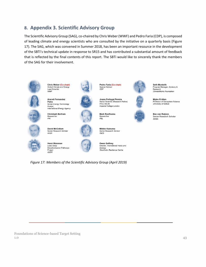
8. Appendix 3. Scientific Advisory Group
The Scientific Advisory Group (SAG), co-chaired by Chris Weber (WWF) and Pedro Faria (CDP), is composed
of leading climate and energy scientists who are consulted by the initiative on a quarterly basis (Figure
17). The SAG, which was convened in Summer 2018, has been an important resource in the development
of the SBTi’s technical update in response to SR15 and has contributed a substantial amount of feedback
that is reflected by the final contents of this report. The SBTi would like to sincerely thank the members
of the SAG for their involvement.
Figure 17: Members of the Scientific Advisory Group (April 2019)

Foundations of Science-based Target Setting 1.0 44
9. Document History
Version Change/update description Date finalized Effective Dates
1.0 First publication April 2019 Not applicable


