Page 1
FP6-IST-2003-506745 CAPANINA Deliverable 14
Mobile link Propagation Aspects, Channel Model and Impairment Mitigation Techniques
Document Number CAP-D14-WP22-UOY-PUB-01 Contractual Date of Delivery to the CEC 1st May 2005
Actual Date of Delivery to the CEC 29th April 2005
Author(s): Candida Spillard (UOY), Emanuela Falletti (POLITO), Jose Delgado Penin (UPC), Jose L. Ruíz-Cuevas (UPC), Marina Mondin (POLITO).
Participant(s) (partner short names): UOY, UPC, POLITO
Editor (Internal reviewer) David Grace (UOY)
Workpackage: WP 2.2
Estimated person months 40
Security (PUBlic, CONfidential, REStricted)
PUB
Nature R-report
CEC Version 1.1
Total number of pages (including cover): 105
Abstract: This report deals with the propagation aspects involved in providing broadband services via High-Altitude
Platforms (HAPs) to users who may be fixed or on trains moving at up to 300 km/hour, for both long-term and event/disaster relief servicing. The ITU has assigned two bands of mm-wave frequencies for these services: one at 47-48 GHz (worldwide) and one at 28-31 GHz (40 countries including Russia and most of Asia). Propagation is predominantly Line-Of Sight, and adversely affected by rain attenuation, for example a margin of 12 dB would be needed to guarantee service availability for 99.9% of the time. For event servicing, the natural variability of weather phenomena has to be taken into account, and an example of the resulting increase in margin is given.
Other considerations include total outages due to railway tunnels, which have been fully characterised in the example of the U.K., loss of line-of-sight due to trees and cuttings, for which statistical models are presented (showing, for example, a good approximation to Rayleigh scattering by trees), and depolarisation due to rain and ice in the event that polarisation re-use may be considered, in which case ice depolarisation may contribute to link outage time. Short-term channel variations such as rain and turbulent scintillation, and Doppler shift and spread, are characterised, and it is shown that for these link geometries at modulations up to 64QAM these factors are unlikely to present a problem.
A Multi-Antenna Channel Simulator has been developed, which models the channel as a tapped delay line, in which each ‘tap’ represents a numerically distinct path. Near each scatterer there is a continuum of small-scale scatterers which give rise to numerically inseparable paths which are modelled as a continuum. The time autocorrelation function is characterised so as to enable the modelling of adaptive fade mitigation techniques, and the spatial autocorrelation function is characterised as it is a necessary input to the design of smart antenna systems for the links.
Finally the various propagation impairment mitigation techniques (PIMTs) are discussed and the applicability of adaptive PIMTs is demonstrated using as an example, adaptive modulation, which is evaluated using a realistic attenuation time-series.
Keyword list: Propagation, Link Margins, Topology, Mobility, Channel model, Fade mitigation
Page 2
Mobile link Propagation Aspects, Channel Model and Impairment Mitigation Techniques CAP-D14-WP22-UOY-PUB-01
DOCUMENT HISTORY
Date Revision Comment Author / Editor Affiliation
29/04/05 01 First issue Candida Spillard UOY
Document Approval (CEC Deliverables only)
Date of
approval Revision Role of approver Approver Affiliation
29/04/05 01 Editor (internal reviewer) David Grace UOY
29/04/05 01 On behalf of scientific board David Grace UOY
29th April 2005 FP6-IST-2003-506745 CAPANINA Page 2 of 105
Page 3
Mobile link Propagation Aspects, Channel Model and Impairment Mitigation Techniques CAP-D14-WP22-UOY-PUB-01
Executive Summary This report constitutes Deliverable 14 of the Propagation workpackage (WP 2.2) of CAPANINA.
The first part describes work contributing to the identification of topology and mobility effects on link margins. This discusses propagation issues, additional to those already covered in previous Ka-band propagation work carried out as part of the HeliNet project (HeliNet Task T2), which need to be considered in the provision of services at Ka-band from High-Altitude Platforms (HAPs) to mobile, broadband users.
The user and backhaul links are at Ka-band (28-31 GHz), meaning propagation is predominantly Line-Of Sight (LOS), and adversely affected by rain attenuation. In the absence of other Propagation Impairment Mitigation Techniques (PIMTs), an attenuation margin of 12 dB would be needed to guarantee service availability for 99.9% of the time, and 32 dB for 99.99%, in a typical hilly mid-latitude location. At the higher bands (47-48GHz) presently specified for Europe, rain attenuation in dB is very approximately double this. The natural variability of meteorological statistics such as rainfall means that for short-term services such as disaster relief and event servicing, even higher margins have to be used if there are fixed guarantee requirements for availability.
The HeliNet project identified rain scatter as a possible issue, but because the antenna beamwidths in the CAPANINA scenario are so narrow, meaning that scattered power arrives in the sidelobes, and it has itself also been attenuated by the rain, interference due to rain scatter is unlikely to present a problem.
The statistics of distributions of the lengths of propagation impairment events such as rain, tunnels, excessive scintillation due to clouds, and trees interrupting the Line-Of-Sight path have been characterised. At Ka-band, tunnels will obscure the signal altogether, while trees will give rise to scattering which, it is shown in a later section, can by modelled as a Rayleigh process with a reasonable degree of accuracy.
Shorter-term variations such as scintillation due to atmospheric turbulence and rain have been characterised and a channel model for events on this timescale has been developed. Scintillation has been shown not to be a relevant issue for CAPANINA links because of their relatively high elevation angle and because 256QAM modulation is not being considered.
Large-scale multipath due to reflections from terrain and buildings is not an issue due to the lack of specular reflections as nearly all relevant surfaces (fields, tarmac, brick walls) are too rough. However, a smaller-scale continuum of multipaths exist due to scattering by objects (such as trees) within a few hundred wavelengths of the Ground Station (GS). These are modelled more rigorously in Chapter 3. The path differences involved are of the order of less than one metre, giving rise to coherence bandwidths in the range of 1 GHz.
The possibility of doubling capacity by polarisation re-use (i.e. the use of right- and left-hand circular polarisation, or vertical and horizontal polarisation) depends upon the extent of depolarisation caused by channel conditions, mainly rain. Typical values are 20 dB of XPD exceeded for 99.9% of the time, and 12 dB for 99.99%. Ice presents an additional problem as it depolarises without attenuating, thus adding to the total time for which adverse conditions prevail, as well as becoming a serious issue if Adaptive Power Control is used at the same time as polarisation re-use.
Doppler effects have been modelled assuming a periodic Doppler shift. Neither HAP nor train vibrations are rapid enough to cause a significant Doppler shift, and the HAP and train travelling velocities will result in Doppler shifts in the KHz range. Doppler spread will be very small, in the range of a few tens of Hz, due to the absence of large-scale, i.e. separable, multipath components.
The conclusions of the general propagation considerations are that the main issues are attenuation due to rain, loss of signal altogether due to railway tunnels, and loss of Line-of-Sight path due to trees and railway cuttings. Depolarisation due to ice may be an issue if polarisation re-use is envisaged, and turbulent scintillation may be an issue if modulation schemes of a higher order than 64QAM are contemplated, or coverage area expanded to the extent of including elevation angles of less than 10o.
29th April 2005 FP6-IST-2003-506745 CAPANINA Page 3 of 105
Page 4
Mobile link Propagation Aspects, Channel Model and Impairment Mitigation Techniques CAP-D14-WP22-UOY-PUB-01
There follows a description of the Multi-Antenna Channel Simulator, which models the channel as a tapped delay line, in which each ‘tap’ represents a numerically distinct path via a large-scale scattering or reflecting object. Near each scatterer there is a continuum of small-scale scatterers which give rise to numerically inseparable paths which are modelled as a continuum. The model takes into account the time autocorrelation function of he channel, which is necessary in the implementation of adaptive PIMTs, and the space autocorrelation function, which must be characterised realistically if one is to evaluate smart antenna systems for the links. For all but dense urban paths there is only one tap on the channel, because no surfaces except the glass and smooth concrete typical of central urban buildings are smooth enough to give specular reflections at Ka-band frequencies. Results of typical channel characteristics are given, showing for example how accurately scattering from trees can be modelled as a Rayleigh process. In the absence of trees Ricean conditions prevail, with typical Rica factors between 15 and 21 dB.
The final part of the report discusses and evaluates different Propagation Impairment Mitigation Techniques, based on diversity, signal processing and adaptive considerations. The performance of a system implementing an adaptive PIMT has been simulated using realistic time-series attenuation data generated using a Markov-like simulation of rain rates. This analysis shows that adaptive PIMT in this scenario is a feasible solution for concatenated digital transmission, by using a time series generator. The performance improves as the BER value decreases, but the values of Eb/ No are only increased around 0.5 dB. It is possible to reduce these values using a concatenated coding based on Turbocodes.
29th April 2005 FP6-IST-2003-506745 CAPANINA Page 4 of 105
Page 5
Mobile link Propagation Aspects, Channel Model and Impairment Mitigation Techniques CAP-D14-WP22-UOY-PUB-01
TABLE OF CONTENTS
EXECUTIVE SUMMARY ......................................................................................................... 3
1 INTRODUCTION............................................................................................................... 9 1.1 The CAPANINA Scenario ...........................................................................................................9 1.2 Structure of the report...............................................................................................................10
2 TOPOLOGY AND MOBILITY EFFECTS ....................................................................... 11 2.1 Introduction ...............................................................................................................................11 2.2 Basic Link Margins....................................................................................................................11 2.2.1 Variability of Link Margins ......................................................................................................14
2.3 Link Outage Durations ..............................................................................................................15 2.3.1 Rain ........................................................................................................................................15 2.3.2 Clouds and Excessive scintillation .........................................................................................17 2.3.3 Cuttings and Tunnels .............................................................................................................17 2.3.4 Trees ......................................................................................................................................19
2.4 Short-term Variations................................................................................................................20 2.4.1 Scintillation .............................................................................................................................20
2.4.1.1 Effect on amplitude........................................................................................................................ 20 2.4.1.2 Effect on Angle-of-arrival ............................................................................................................. 21 2.4.1.3 Effect on phase .............................................................................................................................. 21
2.4.2 Channel model for short-term variations................................................................................24 2.4.3 Typical outputs .......................................................................................................................26
2.5 The significance of Multipath ....................................................................................................27 2.5.1 Terrain multipath ....................................................................................................................27 2.5.2 Reflections from buildings and other structures.....................................................................29
2.6 Polarisation ...............................................................................................................................29 2.6.1 Effect of Rain on XPD ............................................................................................................30 2.6.2 Effect of Ice on XPD...............................................................................................................31 2.6.3 Methods for the improvement of XPD....................................................................................33
2.7 Doppler Studies ........................................................................................................................33 2.7.1 Origins of the Doppler effect ..................................................................................................34 2.7.2 Signal distortion caused by the Doppler effect ......................................................................35 2.7.3 Theoretical considerations .....................................................................................................35
2.7.3.1 Distortion as additional modulation............................................................................................... 35 2.7.3.2 Distortion of the symbol rate ......................................................................................................... 37
2.7.4 Simulation of the Doppler effect .............................................................................................38 2.7.5 Simulation results...................................................................................................................39 2.7.6 Significance of Doppler effect ................................................................................................52
2.8 Conclusions ..............................................................................................................................53
3 THE MULTI-ANTENNA CHANNEL SIMULATOR ......................................................... 55 3.1 Introduction ...............................................................................................................................55
29th April 2005 FP6-IST-2003-506745 CAPANINA Page 5 of 105
Page 6
Mobile link Propagation Aspects, Channel Model and Impairment Mitigation Techniques CAP-D14-WP22-UOY-PUB-01
3.2 Problem Geometry....................................................................................................................56 3.3 Numerical Implementation........................................................................................................58 3.4 The MATLAB files.....................................................................................................................60 3.4.1 Function Demo1Main.m.........................................................................................................62 3.4.2 Function MAMatrixChannel.m................................................................................................63 3.4.3 Data files Cap_R_xx.m..........................................................................................................64
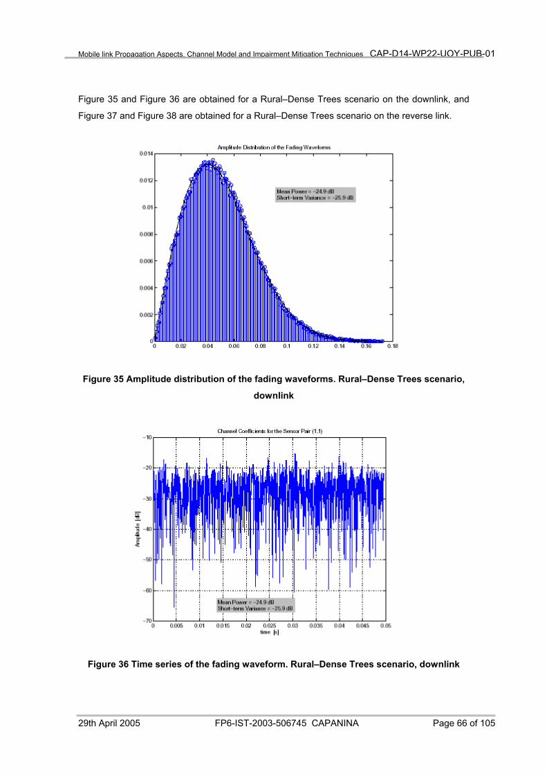
3.5 Simulation Results ....................................................................................................................65 3.6 Conclusion ................................................................................................................................68
4 PROPAGATION IMPAIRMENT MITIGATION TECHNIQUES ....................................... 68 4.1 Introduction ...............................................................................................................................68 4.1.1 Diversity techniques ...............................................................................................................69
4.1.1.1 Spatial diversity ............................................................................................................................. 69 4.1.1.2 Frequency diversity ....................................................................................................................... 70
4.1.2 Signal processing techniques ................................................................................................71 4.1.3 Adaptive Techniques..............................................................................................................71
4.1.3.1 Adaptive TDMA............................................................................................................................ 71 4.1.3.2 Adaptive Uplink/Downlink Power Control ................................................................................... 71 4.1.3.3 Adaptive antennas/beam-shaping .................................................................................................. 72 4.1.3.4 Adaptive Modulation..................................................................................................................... 72
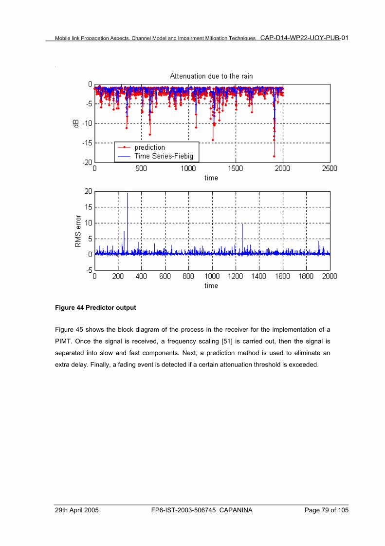
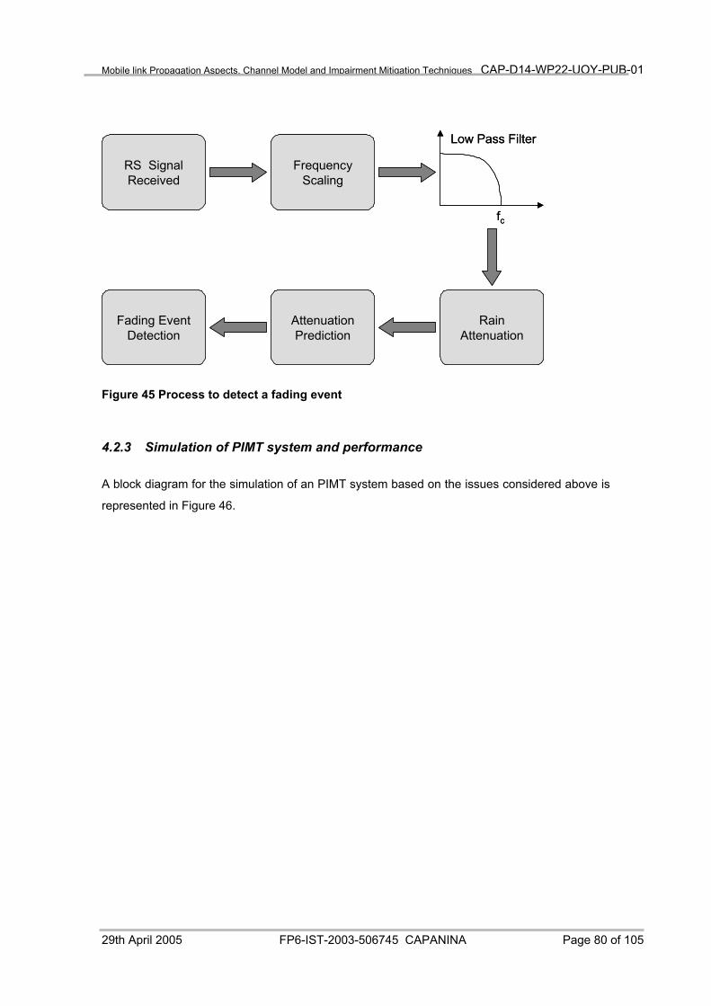
4.2 Performance analysis of a PIMT: Adaptive modulation/coding................................................74 4.2.1 Filtering the time series ..........................................................................................................75 4.2.2 Implementation of a predictor ................................................................................................77 4.2.3 Simulation of PIMT system and performance........................................................................80
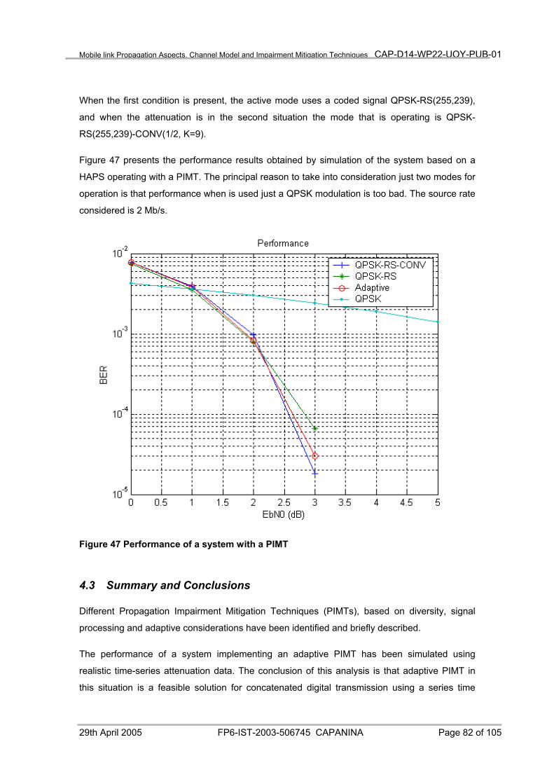
4.3 Summary and Conclusions.......................................................................................................82
5 CONCLUSIONS.............................................................................................................. 83
6 REFERENCES................................................................................................................ 85
7 APPENDIX: DETAILS OF THE CHANNEL SIMULATOR MODEL ............................... 91
29th April 2005 FP6-IST-2003-506745 CAPANINA Page 6 of 105
Page 7
Mobile link Propagation Aspects, Channel Model and Impairment Mitigation Techniques CAP-D14-WP22-UOY-PUB-01
LIST OF ACRONYMS
CDF Cumulative Distribution Function
CINR Carrier to Interference plus Noise Ratio
CPA Co-Polar Attenuation
DSD Drop Size Distribution
FMT Fade Mitigation Technique
FSPL Free-Space Path Loss
GS Ground Station
HAP High Altitude Platform
IPL Inter-Platform Link
ITU-R International Telecommunications Union – Radio communications sector
PIMT Propagation Impairment Mitigation Technique
RB Bit Rate
RET Radiative Energy Transfer
XPD Cross-Polar Degradation
XPI Cross-Polar Isolation
29th April 2005 FP6-IST-2003-506745 CAPANINA Page 7 of 105
Page 8
Mobile link Propagation Aspects, Channel Model and Impairment Mitigation Techniques CAP-D14-WP22-UOY-PUB-01
LIST OF SYMBOLS
aTX(>) transmitter array steering vector in the direction >
÷ the set of complex numbers
f0 carrier frequency (Hz)
h(.,t) path impulse response at time t
M number of antennas at the receiver
N number of antennas at the transmitter
p position vector of array element
RB bit rate (Hz)
RTD Time delay path autocorrelation matrix
s vector of transmitted signals (one component per element of transmitter array)
u transmitted signal
(x,y,z) position vector
t time (sec)
v* beamforming weight vector
"sc, Nsc attenuation and phase rotation of scattered radiation
LTX velocity vector of transmitter
LRX velocity vector of receiver
2 angle of arrival
. tap delay
> angle of departure
J0 LOS propagation time (sec)
P vector consisting of Angle-of-Arrival, Angle-of-Departure and Doppler angle
R Doppler angle
29th April 2005 FP6-IST-2003-506745 CAPANINA Page 8 of 105
Page 9
Mobile link Propagation Aspects, Channel Model and Impairment Mitigation Techniques CAP-D14-WP22-UOY-PUB-01
1 Introduction
This report deals with the propagation aspects of the provision of broadband services to mobile
users via High-Altitude Platforms (HAPs). The ITU has assigned two bands of mm-wave
frequencies for broadband services from HAPs: one at 47-48 GHz (worldwide) and one at 28-31
GHz (40 countries including Russia and most of Asia). These bands have the advantage over
lower microwave frequencies of few, if any, incumbent operators and wide bandwidth, and have
potential to provide very high capacity. For the purposes of this report, only the lower of the two
bands (28-31 GHz) is considered, however given the similarity of propagation mechanisms in
the two bands, the findings are easily adapted to the generally harsher propagation conditions
of the higher band.
1.1 The CAPANINA Scenario
A block diagram of the CAPANINA scenario for delivering broadband services from HAPs is
shown in Figure 1.
31/28GHz, (47/48GHz)+ optical backhaul & interplatform
Up to 120Mbit/s
17-22km
Fixed BFWA particularly for rurallocations
Moving Train
Up to 300km/h
WLAN
31/28GHz, (47/48GHz)+ optical backhaul & interplatform
Up to 120Mbit/s
17-22km
Fixed BFWA particularly for rurallocations
Moving Train
Up to 300km/h
WLAN
Up to 120Mbit/s
17-22km
Fixed BFWA particularly for rurallocations
Moving Train
Up to 300km/h
Moving Train
Up to 300km/hUp to 300km/h
WLANWLAN
Figure 1 The CAPANINA scenario
Broadband Fixed Wireless Access (BFWA) links are provided via HAPs to users in remote
locations with a similar, cellular network architecture to that described in the HeliNet project [1],
with the aggregate data rate in each cell being 120 MB/s to be shared on demand between all
users in that cell. Multiple HAPs, with mm-wave or optical Inter-Platform Links (IPLs), may be
29th April 2005 FP6-IST-2003-506745 CAPANINA Page 9 of 105
Page 10
Mobile link Propagation Aspects, Channel Model and Impairment Mitigation Techniques CAP-D14-WP22-UOY-PUB-01
deployed either to increase capacity within their common footprint area, or to extend coverage
to an entire region over many footprints. Satellite or terrestrial backhaul can be used for
connection to other networks. Connection at the user end will either be direct to the home or
business, or to a WLAN access node, serving a group of users (e.g. a village or street).
In addition, the CAPANINA scenario offers Broadband services at similar data rates, to users
interfacing with on-board wireless LAN base stations on trains travelling at speeds of up to 300
km/hr. The high data rate and the velocity of the vehicle present a need for additional
information about the propagation channel.
For IPL and backhaul infrastructure, optical free space transmission technology can be used as
it is capable of delivering very high data rates in clear air, using spectrum that is free to the
operator. HAPs will be situated well above the clouds so optical interplatform links should in
principle be permanently available. This also affords the chance of exploiting HAP spatial
diversity to ensure an increased likelihood of backhaul to the ground in clear air. However it will
be augmented by mm-wave band backhaul to provide a link at reduced data rate for critical
traffic.
The nature of the services determines some of the Propagation Impairment Mitigation
Techniques (PIMTs) that can be used. Services offered include Broadband Internet access to
residential/soho, ad-hoc networks for special events and disaster recovery, broadband
connection WiFi on trains and coaches, WiFi backhauling, content distribution, streaming media
and TV broadcasting. Some of these are amenable to caching or retransmission, while some
are amenable to other PIMTs such as transmission at reduced data rates during adverse
conditions.
1.2 Structure of the report
Section 2 builds on work already undertaken as part of the EU framework 5 project HeliNet [1],
which dealt with some of the propagation mechanisms involved in the provision of lower data-
rate services to fixed users. The section deals with extra factors, such as Doppler shift, which
must be considered when users are moving, and scintillation, which may have to be considered
if coverage areas are to be extended outwards from the Sub-Platform Point (SPP) to fringe
areas where the HAP is seen at a low elevation angle.
In Section 3 we describe a numerical Channel Simulator which has been developed to consider
the time and space autocorrelation characteristics of the channel. Characterisation of the
temporal variations is necessary in order to implement certain adaptive Propagation Impairment
29th April 2005 FP6-IST-2003-506745 CAPANINA Page 10 of 105
Page 11
Mobile link Propagation Aspects, Channel Model and Impairment Mitigation Techniques CAP-D14-WP22-UOY-PUB-01
Mitigation Techniques (PIMTs), whereas knowledge of the spatial autocorrelation
characteristics is needed in the design and implementation of smart antennas for the links.
The final section deals with the PIMTs which may be applied in the case of a HAP network
providing broadband services.
2 Topology and Mobility Effects
2.1 Introduction
For the purpose of channel modelling, we start with longer-term effects, such as rain fades,
which are used in the ascertaining of mean link availabilities over long periods. It is also
necessary to quantify how appropriate these long-term statistics are when applied to a short-
term scenario, such as event servicing.
We then move on to consider the durations of fade and other propagation impairment events,
such as those due to tunnels, which at these frequencies cut out the signal altogether, and trees,
which give rise to attenuation and scattering. Knowledge of these durations enables us to
incorporate models of each single channel state (e.g. ‘Attenuated by trees’) into a complete
channel model.
Finally we must evaluate the effects of short-term phenomena, such as scintillation and
reflection. These are simulated using numerical channel models in order to evaluate the
effectiveness of dynamic Propagation Impairment Mitigation Techniques (PIMTs). In this section,
part 2 deals with long-term effects, part 3 with short-term effects, part 4 describes a channel
simulator for short and long-term effects and the remaining parts deal with issues which have
both short- and long-term effects.
2.2 Basic Link Margins
The calculation of link margins for static link geometry is similar to that for HeliNet [1], [2]
because of the similar link geometry. It is envisaged, at least initially, that the cellular pattern
developed in that project [3] will be used for the user links, with steerable Ground Station (GS)
antennas of beamwidths of a few degrees.
29th April 2005 FP6-IST-2003-506745 CAPANINA Page 11 of 105
Page 12
Mobile link Propagation Aspects, Channel Model and Impairment Mitigation Techniques CAP-D14-WP22-UOY-PUB-01
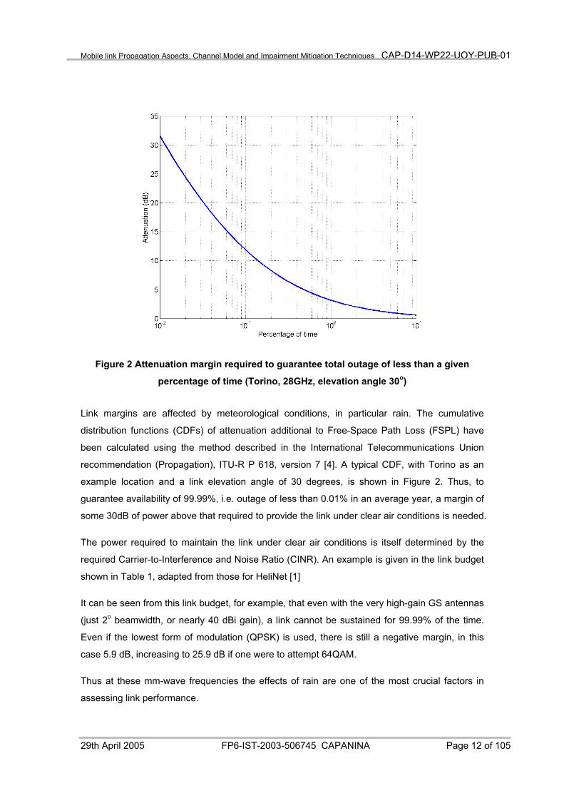
Figure 2 Attenuation margin required to guarantee total outage of less than a given
percentage of time (Torino, 28GHz, elevation angle 30o)
Link margins are affected by meteorological conditions, in particular rain. The cumulative
distribution functions (CDFs) of attenuation additional to Free-Space Path Loss (FSPL) have
been calculated using the method described in the International Telecommunications Union
recommendation (Propagation), ITU-R P 618, version 7 [4]. A typical CDF, with Torino as an
example location and a link elevation angle of 30 degrees, is shown in Figure 2. Thus, to
guarantee availability of 99.99%, i.e. outage of less than 0.01% in an average year, a margin of
some 30dB of power above that required to provide the link under clear air conditions is needed.
The power required to maintain the link under clear air conditions is itself determined by the
required Carrier-to-Interference and Noise Ratio (CINR). An example is given in the link budget
shown in Table 1, adapted from those for HeliNet [1]
It can be seen from this link budget, for example, that even with the very high-gain GS antennas
(just 2o beamwidth, or nearly 40 dBi gain), a link cannot be sustained for 99.99% of the time.
Even if the lowest form of modulation (QPSK) is used, there is still a negative margin, in this
case 5.9 dB, increasing to 25.9 dB if one were to attempt 64QAM.
Thus at these mm-wave frequencies the effects of rain are one of the most crucial factors in
assessing link performance.
29th April 2005 FP6-IST-2003-506745 CAPANINA Page 12 of 105
Page 13
Mobile link Propagation Aspects, Channel Model and Impairment Mitigation Techniques CAP-D14-WP22-UOY-PUB-01
Table 1 Link budget for CAPANINA user link
1 Transmitter (HAP)2 Power per carrier (dBm) a3 Antenna beamwidth - theta (degrees)4 Antenna beamwidth - phi (degrees)5 Antenna electrical efficiency6 Antenna gain (dBi) 29.3 b7 Antenna feed loss (dB) c8 HAP EIRP (dBm) 58.3 d=a+b-c9
10 Receiver (Ground Station)11 The Boltzmann Constant (dBJ/K) -228.612 Noise Temperature (K)13 Thermal noise density (dBm/Hz) -173.8 e14 Receiver noise figure (dB) f15 Receiver noise density (dBm/Hz) -168.8 g=e+f16 Receiver interference noise density (dBm/Hz) -168.8 j = g17 Total effective noise density (dBm/Hz) -165.8 k= 10*log(10^(g/10)+10^(j/10))1819 Antenna beamwidth (degrees)20 Antenna electrical efficiency21 Antenna gain (dBi) 39.4 l22 Cable loss at ground station m23 Maximum C/(Io+No) (dBHz) 261.5 o=d-k+l-m2425 Modulation Scheme26 Required Eb/No (BER 10-9) ab27 Bit/symbol2829 Bandwidth (MHz)30 Code Rate aj31 Data Rate (Mbit/s) (25% rolloff) 120 80 60 20 ad32 Data Rate (dBbit/s) 80.8 79.0 77.8 73.0 p33 Required C/(Io+No) (dBHz) 100.8 95.0 91.8 80.8 ae=ab+p3435 Maximum allowed losses (dB) 160.7 166.4 169.7 180.7 q=o-ae3637 Link Parameters38 Frequency (GHz)39 Wavelength (m) 0.01140 Ground Distance (km)41 Platform Height (km)4243 LOS Distance (km) 34.4844 FSPL (dB) 152.1 r45 Misc Atmospheric Losses (dB) s46 Edge of cell and antenna beam losses sa47 Clear air losses (dB) 157.8 t=r+s+sa4849 Received margin clear air (dB) 2.9 8.6 11.9 22.9 u=q-t50 Minimum required transmit power clear air (dBm) 27.1 21.4 18.1 7.151
User Link for High Rate Broadband Services at 28GHz, Torino
30.03.88.2
0.95
1.0
300.0
5.0
2.00.95
2.0
64QAM 16QAM 8AMPM QPSK20 16 14 7.86 4 3 2 ac
25.0 25.0 25.0 25.01.00 1.00 1.00 0.50
28.0
30.017.0
0.75.0
29th April 2005 FP6-IST-2003-506745 CAPANINA Page 13 of 105
Page 14
Mobile link Propagation Aspects, Channel Model and Impairment Mitigation Techniques CAP-D14-WP22-UOY-PUB-01
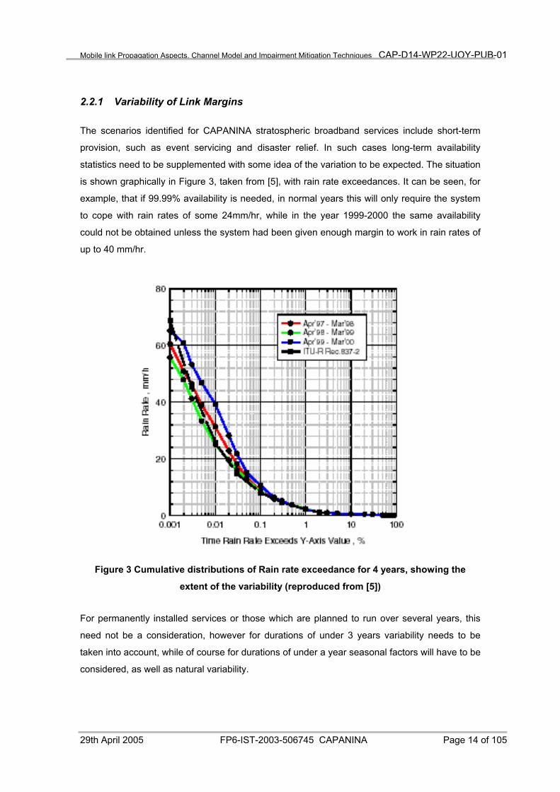
2.2.1 Variability of Link Margins
The scenarios identified for CAPANINA stratospheric broadband services include short-term
provision, such as event servicing and disaster relief. In such cases long-term availability
statistics need to be supplemented with some idea of the variation to be expected. The situation
is shown graphically in Figure 3, taken from [5], with rain rate exceedances. It can be seen, for
example, that if 99.99% availability is needed, in normal years this will only require the system
to cope with rain rates of some 24mm/hr, while in the year 1999-2000 the same availability
could not be obtained unless the system had been given enough margin to work in rain rates of
up to 40 mm/hr.
Figure 3 Cumulative distributions of Rain rate exceedance for 4 years, showing the
extent of the variability (reproduced from [5])
For permanently installed services or those which are planned to run over several years, this
need not be a consideration, however for durations of under 3 years variability needs to be
taken into account, while of course for durations of under a year seasonal factors will have to be
considered, as well as natural variability.
29th April 2005 FP6-IST-2003-506745 CAPANINA Page 14 of 105
Page 15
Mobile link Propagation Aspects, Channel Model and Impairment Mitigation Techniques CAP-D14-WP22-UOY-PUB-01
2.3 Link Outage Durations
Given a power, CINR or phase stability requirement for a particular service, the durations of
intervals in which these requirements are not met, need to be quantified. In particular, this is
because the shortest outages may be overcome by some means, thus improving the service
availability for a given link availability.
2.3.1 Rain
The new recommendation ITU-R P.1623 [4] gives number P(d>D|a>A), and time F(d>D|a>A),
distributions of rain outage durations, where these are defined as:
1 P(d>D|a>A), the probability of occurrence of fades of duration d longer than D seconds,
given that the attenuation a is greater than A dB. This probability can be estimated from the
ratio of the number of fades of duration longer than D to the total number of fades observed,
given that the threshold A is exceeded.
2 F(d>D|a>A), the cumulative exceedance probability, or, equivalently, the total fraction
(between 0 and 1) of fade time due to fades of duration d longer than D seconds, given that the
attenuation a is greater than A dB. This probability can be estimated from the ratio of the total
fading time due to fades of duration longer than D given that the threshold A is exceeded, to the
total exceedance time of the threshold.
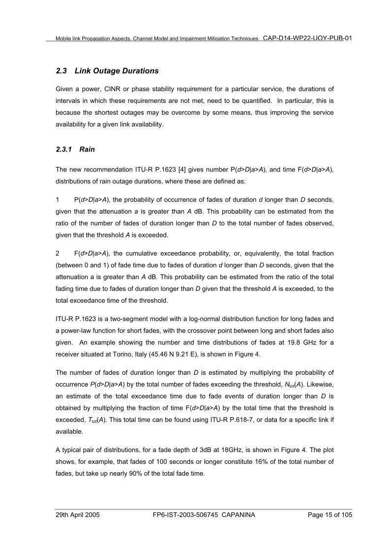
ITU-R P.1623 is a two-segment model with a log-normal distribution function for long fades and
a power-law function for short fades, with the crossover point between long and short fades also
given. An example showing the number and time distributions of fades at 19.8 GHz for a
receiver situated at Torino, Italy (45.46 N 9.21 E), is shown in Figure 4.
The number of fades of duration longer than D is estimated by multiplying the probability of
occurrence P(d>D|a>A) by the total number of fades exceeding the threshold, Ntot(A). Likewise,
an estimate of the total exceedance time due to fade events of duration longer than D is
obtained by multiplying the fraction of time F(d>D|a>A) by the total time that the threshold is
exceeded, Ttot(A). This total time can be found using ITU-R P.618-7, or data for a specific link if
available.
A typical pair of distributions, for a fade depth of 3dB at 18GHz, is shown in Figure 4. The plot
shows, for example, that fades of 100 seconds or longer constitute 16% of the total number of
fades, but take up nearly 90% of the total fade time.
29th April 2005 FP6-IST-2003-506745 CAPANINA Page 15 of 105
Page 16
Mobile link Propagation Aspects, Channel Model and Impairment Mitigation Techniques CAP-D14-WP22-UOY-PUB-01
Figure 4 Number and time distributions of fade durations on a 19.8 GHz link (GS antenna
Height 120m, diameter 1.5m, situated at Torino, Italy)
At present, ITU-R P.1623 takes no account of climatic zones other than indirectly via the CDFs
produced by ITU-R P.617. That is, once the CDF of received signal level has been ascertained,
the distribution of fade lengths within it is location-independent. Investigations carried out as
part of COST programme 280 (Propagation impairment mitigation at mm-wave bands) [6] are
assessing the validity of this assumption. Preliminary findings by Amaya and Rogers [7] indicate
that for Asian sites the distribution of lengths is more heavily biased towards long outages than
for the comparison site in Ottawa.
They also propose that the two-part nature of the fade duration distribution, with different laws
for short and long rain fades, may reflect the dual nature of rainfall, with convective and
stratiform events caused by different physical processes.
Inter-fade durations have as yet not been quantified in such detail, and a general prediction
method has not been established. However Ventouras et al [8] have carried out a detailed study
of fade and interfade durations for satellite beacon signals at frequencies ranging from 18 to 50
GHz at sites in the south of England, and Vilar et al have performed a thorough statistical
analysis of 49 years of rainfall data, recorded near Barcelona at intervals of 10 seconds [9].
Both these studies identified two types of interfade: those between exceedances within an
29th April 2005 FP6-IST-2003-506745 CAPANINA Page 16 of 105
Page 17
Mobile link Propagation Aspects, Channel Model and Impairment Mitigation Techniques CAP-D14-WP22-UOY-PUB-01
‘episode’ of fades (intra-exceedances) and those between episodes (‘inter-exceedances’). This
makes interfade duration statistics more complicated than those of fade duration because two
completely separate models are necessary. However, it turns out that both are log-normal
distributions. The ITU are integrating these and other studies with a view to producing a
universally applicable model for intervals between fades.
2.3.2 Clouds and Excessive scintillation
Excessive scintillation may give rise to outages, not by decreasing carrier level but by causing
synchronisation to be lost in an effect similar to that of phase noise in oscillators, giving rise to
Bit Error Rates (BER) exceeding the minimum specified for that service. Vilar and Catalan [10]
have in fact demonstrated the similarity of the mathematics describing the two phenomena.
This section deals only with the durations of these events treated as outages: their nature
(spectrum, type of disruption caused, etc) is dealt with elsewhere in this report.
Excessive scintillation can occur during rain events and when the path passes through heavy
clouds such as Cumulus (Cu) or Cumulonimbus (Cb), particularly at the edges where water
vapour gradients are steep. The cloud events rarely last long, and their duration is inversely
proportional to mean wind speed. Statistics of cloud cover and movement are available from the
national meteorological organisations who subscribe to the World Meteorological Organisation
(WMO) and are listed on their website [11] under ‘members’.
Scintillation during rain is of course masked by attenuation, such that if the rain rate is high
enough to cause significant scintillation, attenuation has masked the signal. Scintillation during
rain events therefore does not need to be considered here as it does not constitute extra events.
Cloud-induced scintillation is shown, in a later section, not to present a problem for any but the
highest orders of modulation e.g. 256QAM.
2.3.3 Cuttings and Tunnels
At the Ka-band frequencies specified by CAPANINA, propagation is essentially by Line-Of Sight
(LOS), so that there is negligible diffraction into cuttings and tunnels, but instead complete loss
of signal unless alternative provisions, such as relay points at tunnel and station building
openings, have been put in place.
The total outage time, and number and time distributions of outages, can be quantified using
databases of bridge, tunnel and station superstructure lengths obtainable from rail infrastructure
29th April 2005 FP6-IST-2003-506745 CAPANINA Page 17 of 105
Page 18
Mobile link Propagation Aspects, Channel Model and Impairment Mitigation Techniques CAP-D14-WP22-UOY-PUB-01
providers, from maps of routes and even, in the case of the UK, from publications by rail
enthusiasts [12].
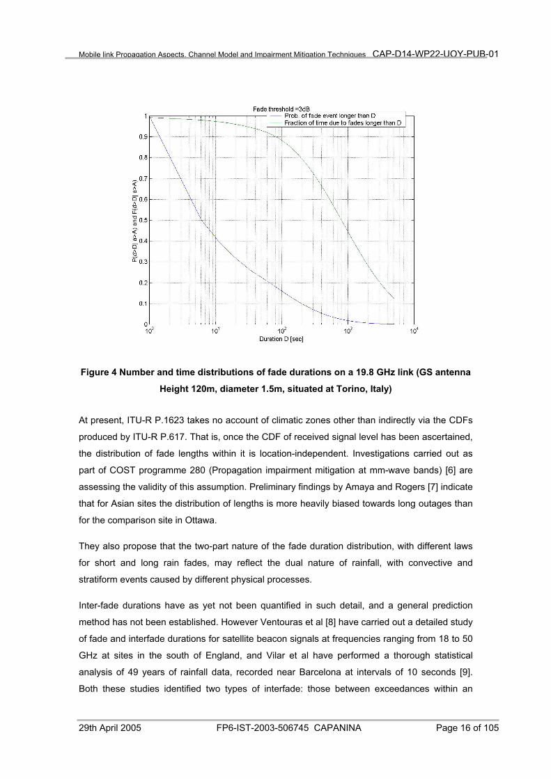
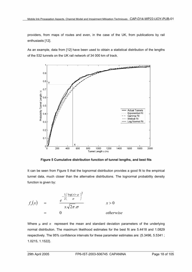
As an example, data from [12] have been used to obtain a statistical distribution of the lengths
of the 532 tunnels on the UK rail network of 34 000 km of track.
Figure 5 Cumulative distribution function of tunnel lengths, and best fits
It can be seen from Figure 5 that the lognormal distribution provides a good fit to the empirical
tunnel data, much closer than the alternative distributions. The lognormal probability density
function is given by:
( )
otherwise
xx
exf
x
s
0
0.2.
2)log(21
=
>=
−
−
σπ
σµ
Where : and F represent the mean and standard deviation parameters of the underlying
normal distribution. The maximum likelihood estimates for the best fit are 5.4418 and 1.0829
respectively. The 95% confidence intervals for these parameter estimates are: {5.3496, 5.5341 ;
1.0215, 1.1522}.
29th April 2005 FP6-IST-2003-506745 CAPANINA Page 18 of 105
Page 19
Mobile link Propagation Aspects, Channel Model and Impairment Mitigation Techniques CAP-D14-WP22-UOY-PUB-01
Data of this kind are useful in simulations to evaluate generically the gains which may be made
using different outage mitigation techniques (antenna diversity, caching etc), whereas for
particular rail routes it is more efficient to use route maps to make it possible to tailor the
mitigation technique (e.g. length of cache, duration for which lost link can be ‘held’, etc) so as to
avoid service outages altogether.
2.3.4 Trees
In woods or cuttings the LOS path will be interrupted by trees. The result is additional
attenuation, scattering, scintillation and depolarisation. Studies undertaken by Ledl et al as part
of the COST 280 project [6] (document as yet only available with password) have measured
Rayleigh-like distributions of signal fading when Ka-band beams are interrupted by trees.
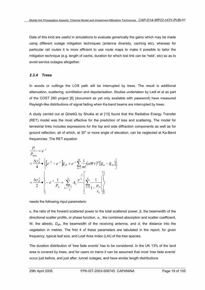
A study carried out at QinetiQ by Shukla et al [13] found that the Radiative Energy Transfer
(RET) model was the most effective for the prediction of loss and scattering. The model for
terrestrial links includes expressions for the top and side diffraction components as well as for
ground reflection, all of which, at 30o or more angle of elevation, can be neglected at Ka-Band
frequencies. The RET equation
[ ] ( ) [ ]
−+−•
∆+
−+−•∆
+
=
∑∑
∑
=+=
−
−
=
−−−
−
N
n
k
n
N
Nk
s
kN
R
Mm
M
m
mM
R
r
s
eAP
e
qqWm
eqee
ePP
k
02
1
ˆ
ˆ2
1
ˆ2
max
1
112
!1
4
µγ
ταγ
τ
τ
τττ
τ
needs the following input parameters:
", the ratio of the forward scattered power to the total scattered power, $, the beamwidth of the
directional scatter profile, or phase function, Ft , the combined absorption and scatter coefficient,
W, the albedo, DgR, the beamwidth of the receiving antenna, and d, the distance into the
vegetation in metres. The first 4 of these parameters are tabulated in the report, for given
frequency, typical leaf size, and Leaf Area Index (LAI) of the tree species.
The duration distribution of ‘tree fade events’ has to be considered. In the UK 13% of the land
area is covered by trees, and for users on trains it can be assumed that most ‘tree fade events’
occur just before, and just after, tunnel outages, and have similar length distributions
29th April 2005 FP6-IST-2003-506745 CAPANINA Page 19 of 105
Page 20
Mobile link Propagation Aspects, Channel Model and Impairment Mitigation Techniques CAP-D14-WP22-UOY-PUB-01
2.4 Short-term Variations
Once the Cumulative Distribution Functions of received signal level over the long term are
available, and the durations of the different types of Propagation Impairment event have been
characterised, shorter-term variations have to be considered.
2.4.1 Scintillation
Turbulent eddies in the atmosphere mix air masses whose temperatures, pressures and
humidities vary slightly, causing small random variations in refractive index. These give rise to
random variations in amplitude, phase and angle-of-arrival of mm-waves on HAP links. All of
these effects increase dramatically at low angles of elevation. At very low elevations (less than
a few degrees), scintillation can merge into atmospheric multipath, which is characterised by
slower, deeper (>10dB) fades and is the result of partial reflections from atmospheric layers or
‘feuillets’ associated with rapid refractivity gradients, causing alternately constructive and
destructive interference. However these need not be considered for CAPANINA link geometries
because the elevation angles are too great (i.e. above 5o).
Here we assume that variations in amplitude and phase due to scintillation can be ‘tracked’ for
demodulation, unless the scintillation is excessive.
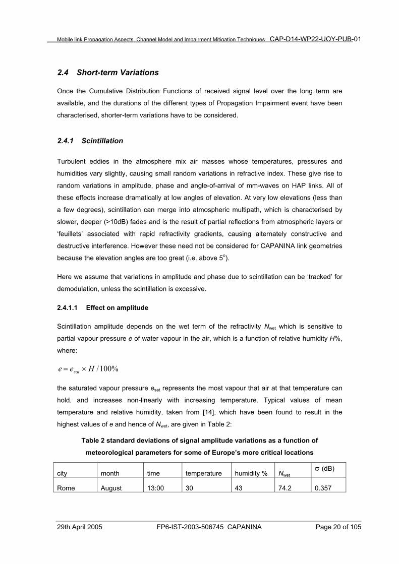
2.4.1.1 Effect on amplitude
Scintillation amplitude depends on the wet term of the refractivity Nwet which is sensitive to
partial vapour pressure e of water vapour in the air, which is a function of relative humidity H%,
where:
%100/Hee sat ×=
the saturated vapour pressure esat represents the most vapour that air at that temperature can
hold, and increases non-linearly with increasing temperature. Typical values of mean
temperature and relative humidity, taken from [14], which have been found to result in the
highest values of e and hence of Nwet, are given in Table 2:
Table 2 standard deviations of signal amplitude variations as a function of
meteorological parameters for some of Europe’s more critical locations
city month time temperature humidity % Nwet σ (dB)
Rome August 13:00 30 43 74.2 0.357
29th April 2005 FP6-IST-2003-506745 CAPANINA Page 20 of 105
Page 21
Mobile link Propagation Aspects, Channel Model and Impairment Mitigation Techniques CAP-D14-WP22-UOY-PUB-01
Rome December 13:00 13 70 47.8 0.272
Rome August 07:00 20 73 74.2 0.357
Rome December 07:00 6 85 38.1 0.240
Gibraltar August 14:30 29 60 98.4 0.434
Nicosia August 14:00 37 35 85.4 0.398
The final column gives the standard deviations of the signal amplitude variations, calculated
following the method described in [4].
2.4.1.2 Effect on Angle-of-arrival
Variations in the angle of arrival are estimated in ITU-R P.834 for frequencies up to 20 GHz,
and by Vilar [15]. The random variations in angle-of-arrival for link elevation 1o are of the order
of 0.1o, and will be considerably more than a magnitude less at 5o of elevation. This is much
less than the minimum antenna beamwidth specified in any CAPANINA HAP link budget, which
is 2o.
The magnitude and rate of change of phase have an important bearing on the choice of
modulation and coding schemes. They are not covered by the ITU.
2.4.1.3 Effect on phase
As previously mentioned, Vilar and Catalan [10] have shown that phase changes due to
atmospheric turbulence can be modelled in a similar way to phase noise in an oscillator. If the
variance of an ensemble of phase shifts )J(N) over a series of time intervals J is given by:
12 ))(( +=∆ bDτφσ τ
where D is the phase diffusion coefficient, then as J increases the variance of the phase errors
increases by a factor t(b+1)/2. The case b=0 represents white FM noise and b=1 represents
flicker FM noise.
Phase noise due to turbulence can be modelled by using b = 2/3. If the phase variations shifts
)J(N) are assumed to have zero mean value then their variance is equivalent to the structure
function of the turbulence, which is given by [16]:
3/522
22 )(246.1)))((( τνλπφσ τ LCrad n
=∆
29th April 2005 FP6-IST-2003-506745 CAPANINA Page 21 of 105
Page 22
Mobile link Propagation Aspects, Channel Model and Impairment Mitigation Techniques CAP-D14-WP22-UOY-PUB-01
where 8 is the wavelength of the radiation, < is the wind speed, L is the path length through the
turbulence and Cn2 is the ‘Refractive index Structure constant’ of the turbulence. The time
interval J is that between preambles (which allow for corrections of the phase of the signal),
which for IEEE802.16 is of the order of 1ms.
The structure constant may vary considerably with atmospheric conditions, between 10-16 m–2/3
when the air is calm, to 10-11 m–2/3 or more at the edges of cumulus (Cu) clouds. At a given
location, it also increases with increasing refractivity gradient, which in turn is dependent on
atmospheric moisture content.
Except for that at the edges of cumulus clouds, turbulence tends to occur in extended layers
within the atmosphere, so that in general the path length L through the turbulence increases
with decreasing elevation angle.
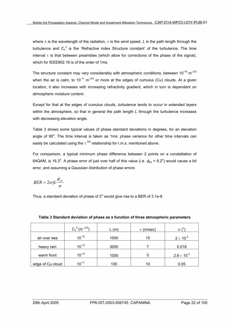
Table 3 shows some typical values of phase standard deviations in degrees, for an elevation
angle of 90o. The time interval is taken as 1ms: phase variance for other time intervals can
easily be calculated using the J 5/6 relationship for r.m.s. mentioned above.
For comparison, a typical minimum phase difference between 2 points on a constellation of
64QAM, is 16.3o. A phase error of just over half of this value (i.e. Npe = 8.2o) would cause a bit
error, and assuming a Gaussian distribution of phase errors:
σφ peerfcBER 2=
Thus, a standard deviation of phase of 2o would give rise to a BER of 3.1e-8.
Table 3 Standard deviation of phase as a function of three atmospheric parameters
Cn2 (m –2/3) L (m) ν (m/sec) σ (o)
air over sea 10-15 1000 15 2 × 10⁻³
heavy rain 10-13 3000 7 0.018
warm front 10-14 1000 5 2.6 × 10⁻³
edge of Cu cloud 10-11 100 10 0.05
29th April 2005 FP6-IST-2003-506745 CAPANINA Page 22 of 105
Page 23
Mobile link Propagation Aspects, Channel Model and Impairment Mitigation Techniques CAP-D14-WP22-UOY-PUB-01
Comparing the standard deviation figures in the final column with the values above, it can be
seen that for these links the effect of atmospheric scintillation on phase alone does not present
a problem for 64QAM.
There is evidence that the ITU model for scintillation in recommendation P.618-7 may
underestimate the problem at Ka-band, because these frequencies are at the very highest of
the measurements on which the model was based.
The turbulence model described by Tatarski [16] results in a spectral density distribution which
is even above a certain corner frequency fc, and falls off below it at a rate of 80/3 dB per decade.
A typical scintillation spectrum derived using the method described by Vanhoenacker at al [17]
based on Tatarski’s theory, for 28 GHz signal with an elevation angle of 30o passing through a
turbulent layer in which the Structure Parameter Cn2 = 10-15 m-2/3 is shown in Figure 6.
Figure 6 Typical scintillation spectrum showing f-80/3 dependence above the corner
frequency
The difficulty in assessing the effects of turbulence lies in evaluating Cn2 which may vary
between 10-16 and 10-12 m-2/3. Decreasing the elevation angle results in a decrease in the corner
frequency, but an overall increase in Power Spectral Density in both halves of the spectrum.
29th April 2005 FP6-IST-2003-506745 CAPANINA Page 23 of 105
Page 24
Mobile link Propagation Aspects, Channel Model and Impairment Mitigation Techniques CAP-D14-WP22-UOY-PUB-01
For elevation angles above 30o such as those in the CAPANINA scenario, and modulation of up
to 64QAM with training sequences every millisecond characteristic of IEEE802.16, the effects
of atmospheric scintillation are not a propagation impairment issue.
2.4.2 Channel model for short-term variations
Figure 7 Block diagram of channel model
The channel model developed for this study is shown in Figure 7. The rain attenuation time-
series generator is based on the time-series generator developed by Fiebig [18] [19].
Segments of the trace of the signal power received are classified as one of three kinds:
Almost constant (C), Monotonically decreasing (D) or Monotonically increasing (U).
According to the analysis of data obtained from the measurements carried out by Fiebig, the
attenuation level at a certain instant depends only on the attenuation in some time )t seconds
before and on the actual type of signal segment (C, D or U). Furthermore, the measured PDFs
of the likelihood P(y/x) for the segments C, D and U has a Gaussian-like shape, where P(y/x) is
the likelihood that the attenuation level is y dB, conditional that it has been x dB )t seconds
before. For these measurements Fiebig uses a value of 64 seconds for )t. The implementation
of this time series generator is based on the scheme shown in Figure 8.
29th April 2005 FP6-IST-2003-506745 CAPANINA Page 24 of 105
Page 25
Mobile link Propagation Aspects, Channel Model and Impairment Mitigation Techniques CAP-D14-WP22-UOY-PUB-01
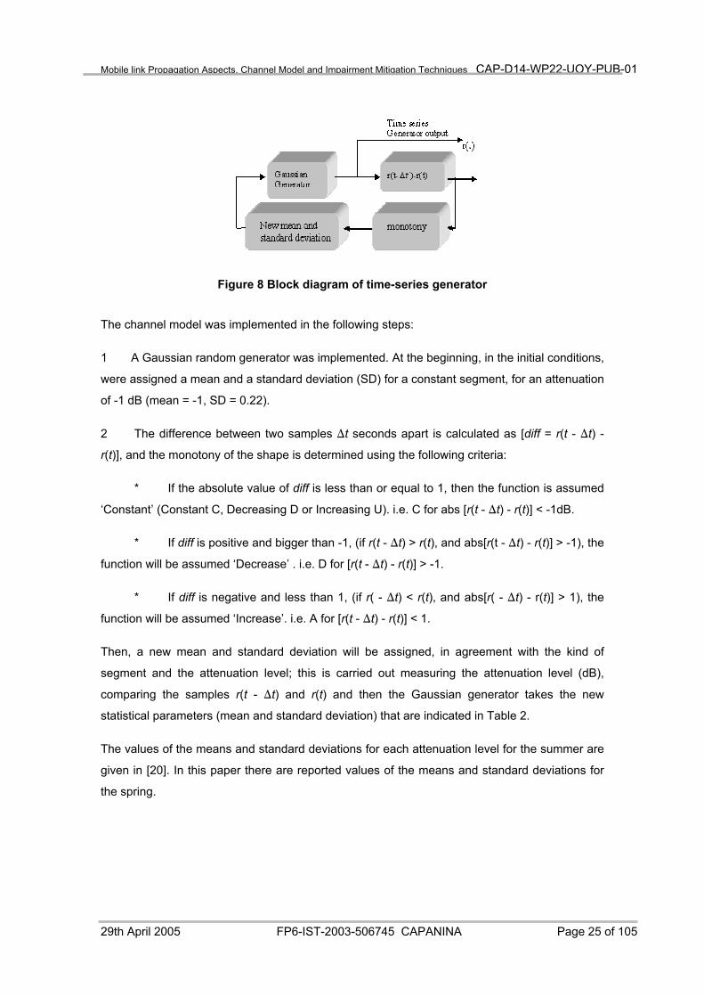
Figure 8 Block diagram of time-series generator
The channel model was implemented in the following steps:
1 A Gaussian random generator was implemented. At the beginning, in the initial conditions,
were assigned a mean and a standard deviation (SD) for a constant segment, for an attenuation
of -1 dB (mean = -1, SD = 0.22).
2 The difference between two samples )t seconds apart is calculated as [diff = r(t - )t) -
r(t)], and the monotony of the shape is determined using the following criteria:
* If the absolute value of diff is less than or equal to 1, then the function is assumed
‘Constant’ (Constant C, Decreasing D or Increasing U). i.e. C for abs [r(t - )t) - r(t)] < -1dB.
* If diff is positive and bigger than -1, (if r(t - )t) > r(t), and abs[r(t - )t) - r(t)] > -1), the
function will be assumed ‘Decrease’ . i.e. D for [r(t - )t) - r(t)] > -1.
* If diff is negative and less than 1, (if r( - )t) < r(t), and abs[r( - )t) - r(t)] > 1), the
function will be assumed ‘Increase’. i.e. A for [r(t - )t) - r(t)] < 1.
Then, a new mean and standard deviation will be assigned, in agreement with the kind of
segment and the attenuation level; this is carried out measuring the attenuation level (dB),
comparing the samples r(t - )t) and r(t) and then the Gaussian generator takes the new
statistical parameters (mean and standard deviation) that are indicated in Table 2.
The values of the means and standard deviations for each attenuation level for the summer are
given in [20]. In this paper there are reported values of the means and standard deviations for
the spring.
29th April 2005 FP6-IST-2003-506745 CAPANINA Page 25 of 105
Page 26
Mobile link Propagation Aspects, Channel Model and Impairment Mitigation Techniques CAP-D14-WP22-UOY-PUB-01
2.4.3 Typical outputs
Figure 9 shows a typical time series generated by the model proposed by Fiebig and
implemented in [21] and [22].
Figure 9 A typical signal level time-series produced by the Fiebig generator
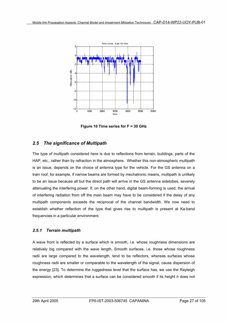
Long term frequency scaling of attenuation allows extension of long term statistics at one
frequency to a different frequency. In this case, the frequency scaling is used for obtaining a
time series for rain attenuation at 30 GHz, from Fiebig´s time series at 40 GHz. For this, we use
the model recommended by the ITU [4]; this model is expressed by:
1 1
2 2
( )( )
A g fA g f
=
where:
( )272.17
72.1
1031)(
fffg
××+=
−
with A1 and A2 being the hydrometeors attenuation in dB at frequencies f1 and f2 in GHz
respectively. Therefore, applying the expression for g(f) to the time series generated, it is
possible to obtain a time series that characterizes the rain attenuation at 30 GHz. This time
series, implemented as explained in [21] and [22], is shown in Figure 10.
29th April 2005 FP6-IST-2003-506745 CAPANINA Page 26 of 105
Page 27
Mobile link Propagation Aspects, Channel Model and Impairment Mitigation Techniques CAP-D14-WP22-UOY-PUB-01
Figure 10 Time series for F = 30 GHz
2.5 The significance of Multipath
The type of multipath considered here is due to reflections from terrain, buildings, parts of the
HAP, etc., rather than by refraction in the atmosphere. Whether this non-atmospheric multipath
is an issue, depends on the choice of antenna type for the vehicle. For the GS antenna on a
train roof, for example, if narrow beams are formed by mechatronic means, multipath is unlikely
to be an issue because all but the direct path will arrive in the GS antenna sidelobes, severely
attenuating the interfering power. If, on the other hand, digital beam-forming is used, the arrival
of interfering radiation from off the main beam may have to be considered if the delay of any
multipath components exceeds the reciprocal of the channel bandwidth. We now need to
establish whether reflection of the type that gives rise to multipath is present at Ka-band
frequencies in a particular environment.
2.5.1 Terrain multipath
A wave front is reflected by a surface which is smooth, i.e. whose roughness dimensions are
relatively big compared with the wave length. Smooth surfaces, i.e. those whose roughness
radii are large compared to the wavelength, tend to be reflectors, whereas surfaces whose
roughness radii are smaller or comparable to the wavelength of the signal, cause dispersion of
the energy [23]. To determine the ruggedness level that the surface has, we use the Rayleigh
expression, which determines that a surface can be considered smooth if its height h does not
29th April 2005 FP6-IST-2003-506745 CAPANINA Page 27 of 105
Page 28
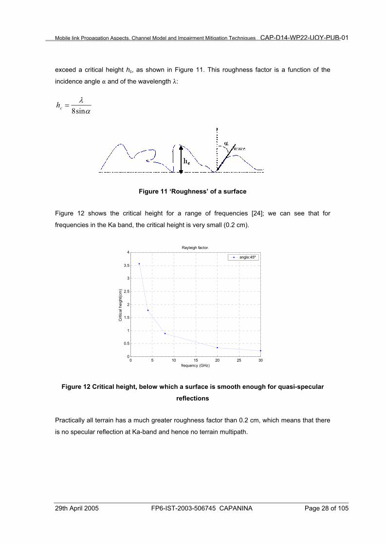
Mobile link Propagation Aspects, Channel Model and Impairment Mitigation Techniques CAP-D14-WP22-UOY-PUB-01
exceed a critical height hc, as shown in Figure 11. This roughness factor is a function of the
incidence angle " and of the wavelength 8:
αλ
sin8=ch
Figure 11 ‘Roughness’ of a surface
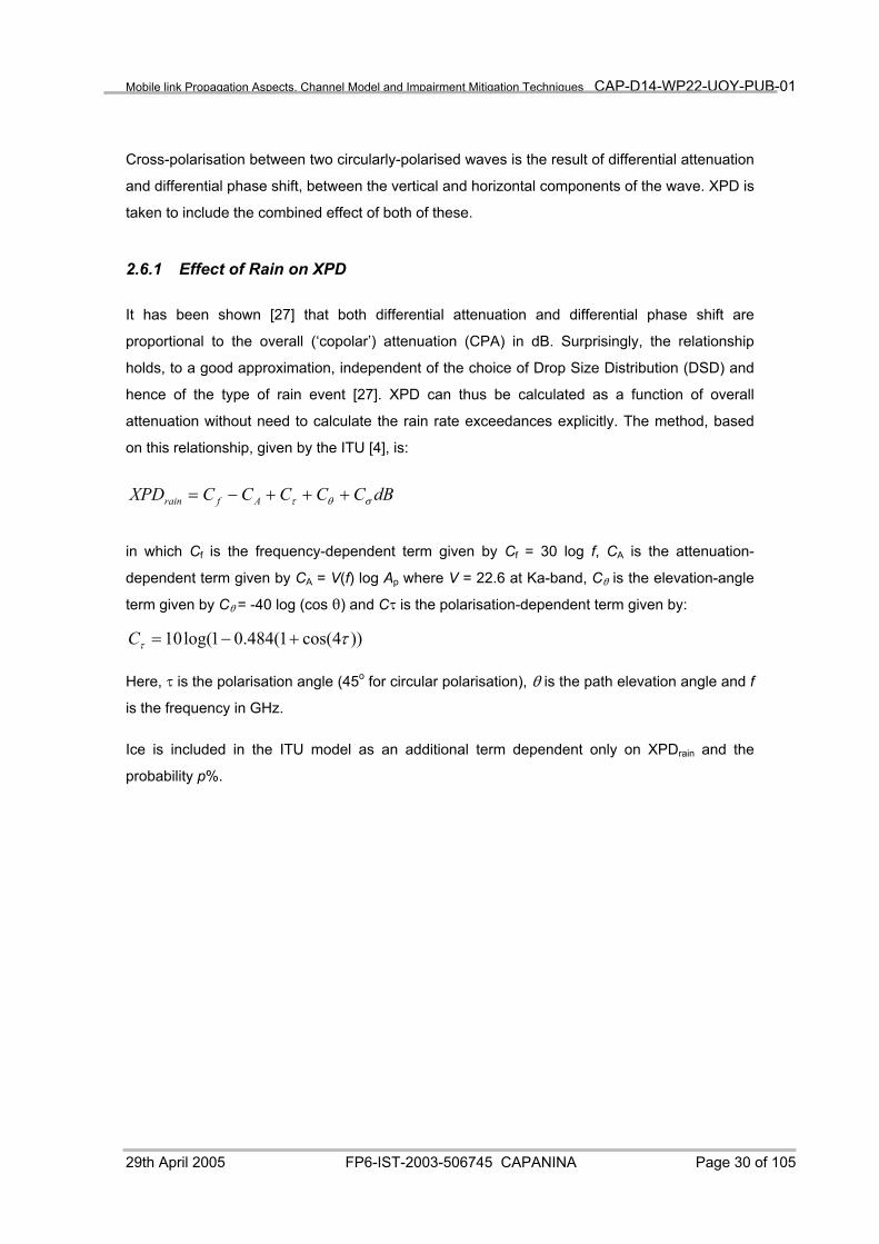
Figure 12 shows the critical height for a range of frequencies [24]; we can see that for
frequencies in the Ka band, the critical height is very small (0.2 cm).
0 5 10 15 20 25 300
0.5
1
1.5
2
2.5
3
3.5
4
frequency (GHz)
Crit
ical
hei
ght(c
m)
Rayleigh factor.
angle:45º
Figure 12 Critical height, below which a surface is smooth enough for quasi-specular
reflections
Practically all terrain has a much greater roughness factor than 0.2 cm, which means that there
is no specular reflection at Ka-band and hence no terrain multipath.
29th April 2005 FP6-IST-2003-506745 CAPANINA Page 28 of 105
Page 29
Mobile link Propagation Aspects, Channel Model and Impairment Mitigation Techniques CAP-D14-WP22-UOY-PUB-01
2.5.2 Reflections from buildings and other structures
Many building materials such as windows, the smoother walls and metal beams (including parts
of the HAP payload) are smooth enough to give rise to specular reflections.
A study by Andreyev and Bugaev [25] reported in COST 280 [6] provides a full-wave model of
the reflected fields. Their results, both measured and modelled, show that a typical wall may
have a reflection co-efficient of up to 98% if the whole of the main beam is incident on the wall
(i.e. 98% of the energy incident on the wall is reflected and may give rise to interference).
However it is important to stress that with the very narrow GS antenna beamwidths specified for
CAPANINA mobile communications, this is unlikely to present a problem.
Analyses of whether reflections from the HAP payload may present a problem are dependent
on the geometry of the mechanical parts of the payload, which have not yet been specified in
enough detail. Reflections from railway infrastructure (power cable supports etc) may in future
be the subject of similar analysis, but some information can be found in [26].
2.6 Polarisation
The possibility exists of doubling link capacity by using the two polarisations for two channels
(polarisation re-use). However certain propagation conditions, such as the presence of ice
crystals and non-spherical raindrops, give rise to cross-polarisation, in the form of an unwanted
power Pxpol at the receiver, as well as the desired power Pcopol. Cross-Polar Discrimination
(XPD) is defined as:
dBPP
XPDcopol
xpollog20=
It is generally acknowledged that, in the absence of any signal processing method for
combining the polarisations to extract the two channels (such as MIMO), at least 25 dB of XPD
is required to sustain a link. The antennas themselves will contribute some radiation in the
unwanted polarisation, ranging from 30dB (boresight) downwards to 20 dB (cell edge) in a
typical horn-lens combination used on the HAP for CAPANINA.
It is assumed that for circular polarisation XPI (cross-polar isolation, or the ratio of desired to
undesired radiation at the receiver) is the same as XPD (defined as the ratio of desired signal at
the receiver to undesired radiation received elsewhere but from the same transmitter).
29th April 2005 FP6-IST-2003-506745 CAPANINA Page 29 of 105
Page 30
Mobile link Propagation Aspects, Channel Model and Impairment Mitigation Techniques CAP-D14-WP22-UOY-PUB-01
Cross-polarisation between two circularly-polarised waves is the result of differential attenuation
and differential phase shift, between the vertical and horizontal components of the wave. XPD is
taken to include the combined effect of both of these.
2.6.1 Effect of Rain on XPD
It has been shown [27] that both differential attenuation and differential phase shift are
proportional to the overall (‘copolar’) attenuation (CPA) in dB. Surprisingly, the relationship
holds, to a good approximation, independent of the choice of Drop Size Distribution (DSD) and
hence of the type of rain event [27]. XPD can thus be calculated as a function of overall
attenuation without need to calculate the rain rate exceedances explicitly. The method, based
on this relationship, given by the ITU [4], is:
dBCCCCCXPD Afrain σθτ +++−=
in which Cf is the frequency-dependent term given by Cf = 30 log f, CA is the attenuation-
dependent term given by CA = V(f) log Ap where V = 22.6 at Ka-band, C2 is the elevation-angle
term given by C2 = -40 log (cos 2) and CJ is the polarisation-dependent term given by:
))4cos(1(484.01log(10 ττ +−=C
Here, J is the polarisation angle (45o for circular polarisation), 2 is the path elevation angle and f
is the frequency in GHz.
Ice is included in the ITU model as an additional term dependent only on XPDrain and the
probability p%.
29th April 2005 FP6-IST-2003-506745 CAPANINA Page 30 of 105
Page 31
Mobile link Propagation Aspects, Channel Model and Impairment Mitigation Techniques CAP-D14-WP22-UOY-PUB-01
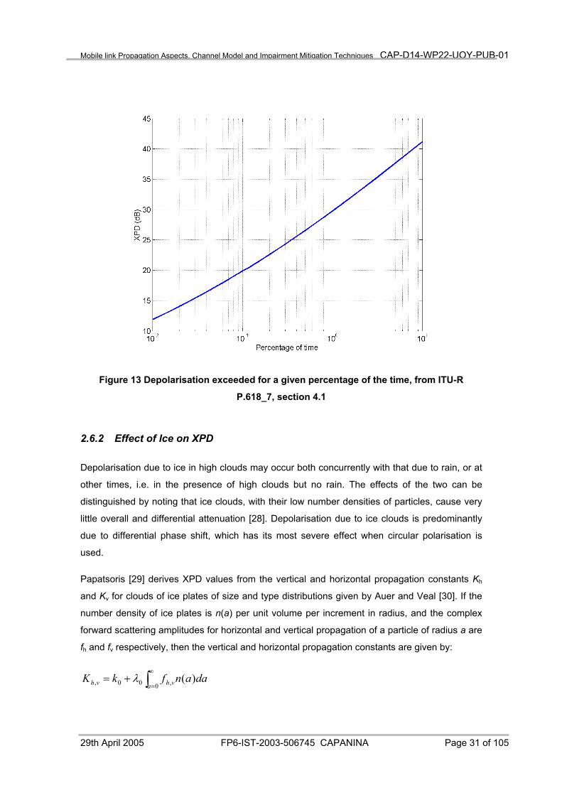
Figure 13 Depolarisation exceeded for a given percentage of the time, from ITU-R
P.618_7, section 4.1
2.6.2 Effect of Ice on XPD
Depolarisation due to ice in high clouds may occur both concurrently with that due to rain, or at
other times, i.e. in the presence of high clouds but no rain. The effects of the two can be
distinguished by noting that ice clouds, with their low number densities of particles, cause very
little overall and differential attenuation [28]. Depolarisation due to ice clouds is predominantly
due to differential phase shift, which has its most severe effect when circular polarisation is
used.
Papatsoris [29] derives XPD values from the vertical and horizontal propagation constants Kh
and Kv for clouds of ice plates of size and type distributions given by Auer and Veal [30]. If the
number density of ice plates is n(a) per unit volume per increment in radius, and the complex
forward scattering amplitudes for horizontal and vertical propagation of a particle of radius a are
fh and fv respectively, then the vertical and horizontal propagation constants are given by:
daanfkKa vhvh )(
0 ,00, ∫∞
=+= λ
29th April 2005 FP6-IST-2003-506745 CAPANINA Page 31 of 105
Page 32
Mobile link Propagation Aspects, Channel Model and Impairment Mitigation Techniques CAP-D14-WP22-UOY-PUB-01
where k0 and 80 are the propagation constant and wavelength in free space. The complex
forward scattering amplitudes can be obtained accurately using Rayleigh scattering theory.
From the propagation constants the differential phase shift ( introduced by travelling a distance
L through the ice is:
LKKj vhe )( −−=γ
from which the cross-polar discrimination is:
θγγθ
2tan)1(tan
+−
=xpd
for linear polarisation at an angle 2 from the horizontal, and
) 45( o=×= θxpdjxpd
for circular polarisation.
The XPD for columns is also derived, but the derivation is more complicated and leads to
interference levels which are insignificant compared to those caused by ice plates.
Cumulative distributions of the ice density exceedances in clouds in a given location are for
obvious practical reasons less readily available than those of rainfall rate exceedances.
However, assumptions can be made about the sequences of cloud types that precede and
follow rain events, for example the sequence Cirrus, Cirrostratus, Altostratus, Altocumulus,
usually precedes the rain on a warm front, and the numbers of fronts passing a given location in
Europe will be readily available from meteorological records. Number densities for Altostratus
and Altocumulus clouds can be approximated by the expression 2.0H104 e –2.0D mm-1m-3, and for
Cumulonimbus (storm clouds) by 3.0H104 D-1 e-2.5Dmm-1m-3 [29], where D is the diameter of the
ice plate in mm.
Fukuchi [31] has derived a relationship between the total depolarisation distribution and that
due to rain alone, by assuming that the Ice Depolarisation Ratio r given by:
%100)(
),(×
≤≤≤
=xXPDP
aAxXPDP xρ
is constant for a given link and rainfall type. This ratio, for a value x of the cross-polar
discrimination, is that of the probability that the XPD is less than x given that attenuation is less
than a corresponding value ax, to the probability that the XPD is less than x in any case. This
gives rise to a correction factor * in the time percentages given by:
29th April 2005 FP6-IST-2003-506745 CAPANINA Page 32 of 105
Page 33
Mobile link Propagation Aspects, Channel Model and Impairment Mitigation Techniques CAP-D14-WP22-UOY-PUB-01
ρ
δ
δ
−=
>×=<
100100
)()( xaAPxXPDP
The correction factor is 10 at or below an attenuation of 10 dB, falling linearly with attenuation to
a value of 1 (i.e. ice makes a negligible contribution to overall depolarisation) at an attenuation
of 40 dB and above. The advantage of this model over that of the ITU [4] is that it takes site
characteristics into account: the attenuations of 10 and 40 dB are translatable directly into
rainfall rates, which in turn, for a given site, translate into time percentages.
2.6.3 Methods for the improvement of XPD
From the calculations in the previous section it can be seen that for most of the time XPD for
circularly-polarised links will exceed 25dB, i.e. links using both polarisations will be sustainable.
However, there are methods available for improving link performance beyond this level.
Extra signal processing can be used, for example MIMO (multiple-In, Multiple-Out) which
reduces the channel crosstalk caused by cross-polar interference by knowing the data in the
cross-talk and subtracting it from the signal. Work on this is ongoing within CAPANINA [32].
A circuit for a compensator which relies on pilot tones but which can operate on links with very
high data rates (3.2GB/s) was designed by Bazak et al [33]. It was found to be able to enhance
values of XPD due to rain of as little as 10dB by as much as a further 10 dB, which in the case
of the HAP links would significantly increase the amount of time for which polarisation re-use
could be made available.
Tomiyasu [34] has proposed the use of vertical dielectric plates for compensating for the fact
that most particles responsible for depolarisation (oblate raindrops, ice plates) have greater
horizontal than vertical dimensions, resulting in a relatively weak and phase-delayed horizontal
component. With an appropriate differential amplitude and phase delay, this will increase XPD
during adverse conditions, at the expense of a slight decrease during clear-air conditions.
2.7 Doppler Studies
The Doppler effect due to aerial platform motion influences the transmitted modulated signal,
which will be distorted. The first effect is the spectral shift caused by the fact that the frequency
changes when transmitter and receiver are moving relatively to each other. Moreover, the
29th April 2005 FP6-IST-2003-506745 CAPANINA Page 33 of 105
Page 34
Mobile link Propagation Aspects, Channel Model and Impairment Mitigation Techniques CAP-D14-WP22-UOY-PUB-01
Doppler frequency shift makes all the signal components vary, and this produces a distortion of
the waveform as a final effect on the modulated signal.
2.7.1 Origins of the Doppler effect
Consider two observers, O and O', whose relative velocity is u; i.e. O' is moving at u m/s with
respect to O. A plane harmonic wave can be described by observer O as a sinusoidal function
sin k(x - ct), where k is the wave number and c is the speed of light in free space. In a different
inertial reference system, co-ordinates x and t must be substituted by x' and t', according to
Lorentz transforms. So observer O' will describe the same wave as sin k'(x' - c t'), where k'
doesn't need to be the same as before. On the other hand, according to relativity laws, c must
be invariant for both O and O' : thus, the following equation holds:
( ) ( tcxkctxk )′−′′=−
This can be rewritten using Lorentz transforms:
( ) ( ) ( )tcxkc
cxtcctxk ′−′′=
−
′+′−
−
′+′2/122
2
2/122 /1/
/1 υυ
υυ
from which the following results
( )
+−
=−
−=′
cck
cckk
/1/1
/1/1
2/122 υυ
υυ
Finally, remembering that T = ck and f = T/2B , this results in:
+−
=′ 2
2
/1/1ccff
υυ
which is known as relativistic Doppler effect. Since both HAP and GS are travelling at much less
than the speed of light, i.e. u<<c, this can be approximated using the binomial expansion in
series, yielding
−≈
+
−≈′
cf
c
cff υ
υ
υ1
/211
/211
2
2
29th April 2005 FP6-IST-2003-506745 CAPANINA Page 34 of 105
Page 35
Mobile link Propagation Aspects, Channel Model and Impairment Mitigation Techniques CAP-D14-WP22-UOY-PUB-01
If a modulated signal is used to carry information, the Doppler effect causes a distortion due to
the consequent carrier shift; moreover, also the symbol timing will be altered.
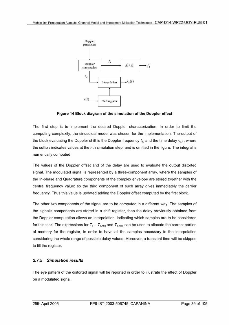
2.7.2 Signal distortion caused by the Doppler effect
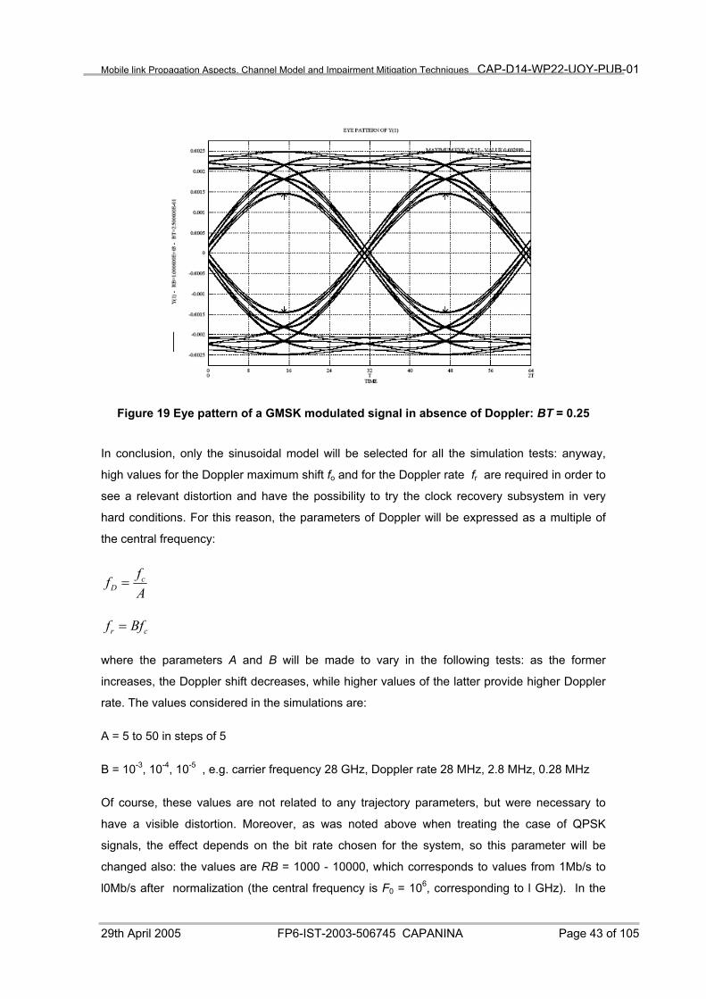
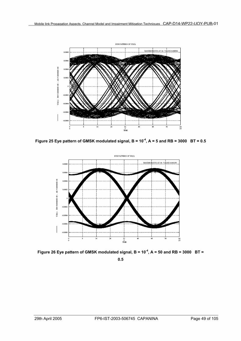
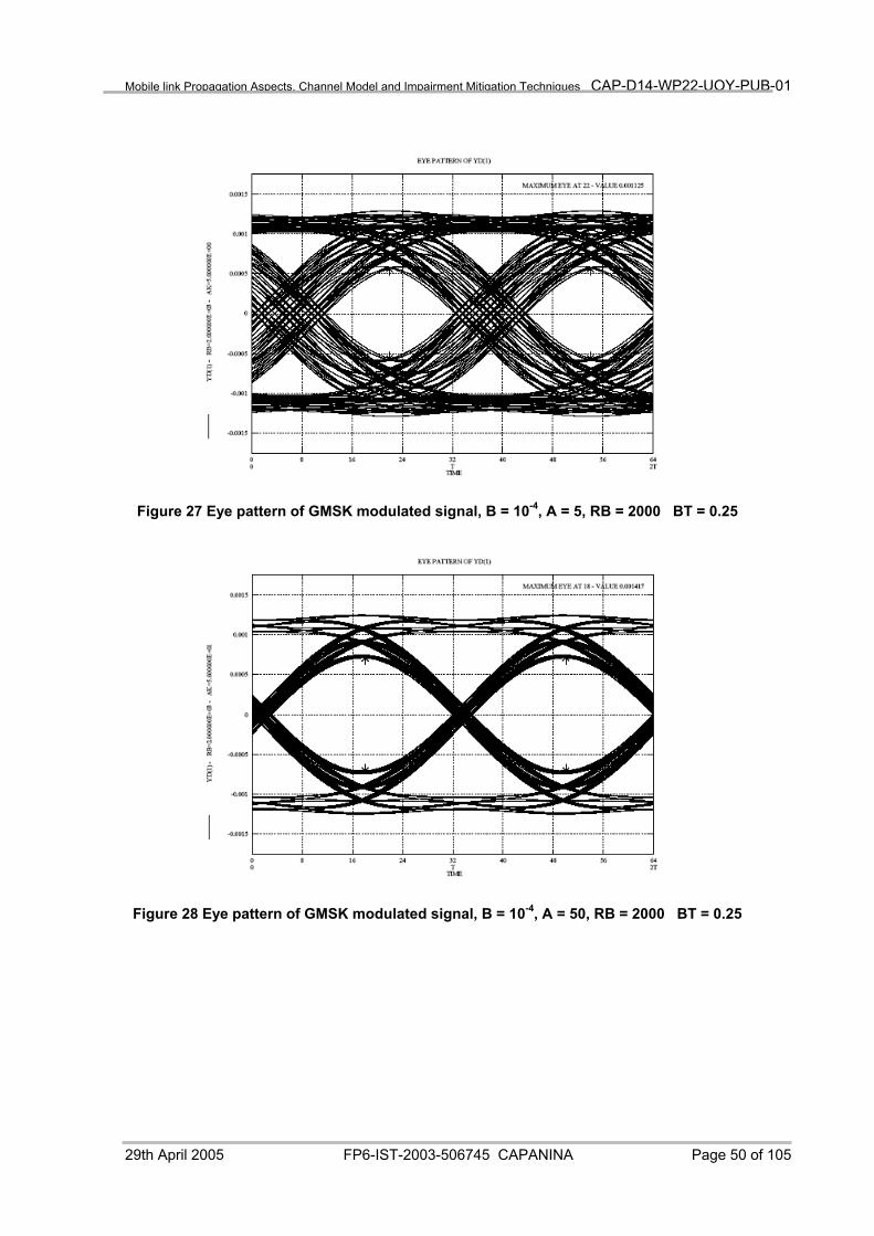
In this section some results will be also illustrated: the GMSK signal will be considered; the eye
pattern will be a useful means to observe the effect in a qualitative way. In addition, a
subroutine will be described, by which the software simulation of the Doppler distortion is
possible.
2.7.3 Theoretical considerations
Let us consider the analytical representation of a modulated signal:
{ }tfj cetxtx π2)(~)( ℜ=
where )(~ tx is the complex envelope of the signal, which bears the information, and fc is the
carrier frequency. If a frequency/phase modulation scheme is considered, the transmitted signal
at the output of the modulator has a constant envelope, say A, and the information symbols are
carried by the carrier phase. The output signal will be of the form
[ )(2cos)( ttfAtx cc ]ϕπ +=
where
(∑ −=k
bk kTtqaht πϕ 2)( )
with h the modulation index and q(t) the phase pulse; ak are the information symbols.
2.7.3.1 Distortion as additional modulation
In presence of Doppler effect the signal will be modulated by the Doppler shift. This distortion
can be represented as a modulator signal having the form fd = fD sin("(t)). Thus, if the signal x(t)
is written in the simplified form x(t) = A cos (2B fc t), where the contribution of data symbols has
been omitted for simplicity, the effect of such frequency modulation will be expressed as
follows:
[ ])(2cos)( ttfAtx dc ϕπ +=
29th April 2005 FP6-IST-2003-506745 CAPANINA Page 35 of 105
Page 36
Mobile link Propagation Aspects, Channel Model and Impairment Mitigation Techniques CAP-D14-WP22-UOY-PUB-01
( )
+= ∫
∞−
t
dc dftfA ζζππ 22cos
( ) ( )
++= ∫
∞−
t
ddc dftfA 022cos ϕζζππ
where Nd(t) is the time-varying phase caused by Doppler effect, which can be written as
( )∫=t
dd dft ζζπϕ 2)(∞−
with fd(.) the Doppler frequency shift. The initial phase Nd(0) can be put to zero without loss of
generality. Now, if the Doppler shift varies sinusoidally, fd(t) can be written as:
( )( )tff Dd αsin=
where "(t) depends on the characterization chosen.
Since the frequency shift introduces a time-varying phase in the modulated signal, this leads to
a time delay Jd(t), where the suffix d indicates that it is caused by the Doppler effect. Thus,
substituting for fd into the expression for x(t), the signal can be expressed as follows:
[ ])(2cos)( ttfAtx dc τπ +=
Comparing this with the previous expression for x(t), the time-varying delay will be:
( ) ( )∫ +=t
dc
d constdff
t0
1 ζζτ
where the constant comes from the integration operation and can be set to zero: the integral
here introduces a ‘memory’ in the non-linearity represented by the Doppler distortion. That is,
when the presence of Doppler alters the lengths of pulses, the effect is cumulative.
From this expression it is clear that the distortion of the transmitted signal strongly depends on
the Doppler characterization considered, since the time delay depends on the final expression
for the Doppler shift fd; in general the integral in the previous equation can be numerically
evaluated but, if the simple case of a sinusoidally varying velocity is considered, then fd can be
substituted with
29th April 2005 FP6-IST-2003-506745 CAPANINA Page 36 of 105
Page 37
Mobile link Propagation Aspects, Channel Model and Impairment Mitigation Techniques CAP-D14-WP22-UOY-PUB-01
( )tfff rDd π2sin=
where fD is the maximum Doppler shift and fr is the Doppler rate. Carrying out the integration
leads to the following expression for the time delay:
( ) ( )( )tfff
ft rrc
Dd π
πτ 2cos1
2−=
where the time dependence of the delay is explicit, whose maximum occurs at t = 1/(2fr) and its
value is:
rc
Dd ff
fπ
τ =max,
2.7.3.2 Distortion of the symbol rate
From the discussion above it is clear that the modulated transmitted signal is distorted by the
Doppler effect since its frequency components are modulated by the Doppler shift. We shall
now see that the duration of an information symbol will also be affected.
Let Ts be the symbol period, expressed in seconds, and Rs = 1/Ts the symbol rate: the former
can be written as a function of the central frequency fc, in Hz, in the form
c
cs f
NT =
where Nc is the ratio between the symbol and the carrier periods. If the Doppler effect is
affecting the system, the Doppler offset will be added to the nominal frequency:
( )tfff dcc +→
where fd(t) is the Doppler shift. Substituting for fc, we have that the actual symbol period is
( ) ( )tffNtT
dc
cs +
=
and becomes a function of time t. Considering the maximum Doppler offset fd(t) a simple
expression can be found for the maximum and the minimum period Ts, max and Ts, min:
Dc
cs ff
NT−
=max,
29th April 2005 FP6-IST-2003-506745 CAPANINA Page 37 of 105
Page 38
Mobile link Propagation Aspects, Channel Model and Impairment Mitigation Techniques CAP-D14-WP22-UOY-PUB-01
Dc
cs ff
NT+
=min,
From the previous equations, the maximum and minimum symbol rate can be derived:
c
Dc
ss N
ffT
R +==
min,max,
1
c
Dc
ss N
ffT
R −==
max,min,
1
as well as the variation with respect to the nominal value of the symbol period as the difference
between Ts and the distorted value. The results are listed below:
( )Dcc
Dcss fff
fNTT+
=− min,
( )Dcc
Dcs fff
fNT+
=max,
from which can be noted that Ts,max - Ts > Ts - Ts,min, thus the variation is not symmetrical and
the range of values in which the actual period is greater that the nominal one results being
larger.
The derivation developed above suggests that the transmitted symbols are compressed or
stretched according to the Doppler shift that is actually distorting the transmitted signal. In the
following section the problem of simulating such effect is discussed, with the aim of deriving a
software subroutine to be included in computer simulation tests.
2.7.4 Simulation of the Doppler effect
In order to simulate the Doppler effect all the discussions developed above are to be taken into
consideration: in fact, the distorted signal should present a distortion of the symbol rate and of
the central frequency according to different Doppler models to be implemented. A block
diagram of the implementation is shown in Figure 14.
29th April 2005 FP6-IST-2003-506745 CAPANINA Page 38 of 105
Page 39
Mobile link Propagation Aspects, Channel Model and Impairment Mitigation Techniques CAP-D14-WP22-UOY-PUB-01
Figure 14 Block diagram of the simulation of the Doppler effect
The first step is to implement the desired Doppler characterization. In order to limit the
computing complexity, the sinusoidal model was chosen for the implementation. The output of
the block evaluating the Doppler shift is the Doppler frequency fd,i and the time delay Jd,i , where
the suffix i indicates values at the i-th simulation step, and is omitted in the figure. The integral is
numerically computed.
The values of the Doppler offset and of the delay are used to evaluate the output distorted
signal. The modulated signal is represented by a three-component array, where the samples of
the In-phase and Quadrature components of the complex envelope are stored together with the
central frequency value: so the third component of such array gives immediately the carrier
frequency. Thus this value is updated adding the Doppler offset computed by the first block.
The other two components of the signal are to be computed in a different way. The samples of
the signal's components are stored in a shift register, then the delay previously obtained from
the Doppler computation allows an interpolation, indicating which samples are to be considered
for this task. The expressions for Ts – Ts,min and Ts,max can be used to allocate the correct portion
of memory for the register, in order to have all the samples necessary to the interpolation
considering the whole range of possible delay values. Moreover, a transient time will be skipped
to fill the register.
2.7.5 Simulation results
The eye pattern of the distorted signal will be reported in order to illustrate the effect of Doppler
on a modulated signal.
29th April 2005 FP6-IST-2003-506745 CAPANINA Page 39 of 105
Page 40
Mobile link Propagation Aspects, Channel Model and Impairment Mitigation Techniques CAP-D14-WP22-UOY-PUB-01
Figure 15 Eye pattern of an ideal QPSK modulated signal in absence of Doppler
The first example is a QPSK signal, whose ideal eye pattern is illustrated in Figure 15. The
pulse is rectangular, so in computer simulations the zero-crossing with a vertical slope presents
a serious problem. Thus an approximation is necessary, and a trapezoidal pulse is instead
chosen for numerical representation of such a signal: the sample corresponding to the zero-
crossing is forced to be zero. In this way, when the autocorrelation is computed as the output of
the matched filter, the input is not rectangular and the output will not be correct: this effect is
clear from the figure, where a trapezoidal waveform can be recognized.
29th April 2005 FP6-IST-2003-506745 CAPANINA Page 40 of 105
Page 41
Mobile link Propagation Aspects, Channel Model and Impairment Mitigation Techniques CAP-D14-WP22-UOY-PUB-01
Figure 16 Eye pattern of QPSK signal in presence of Doppler
However, what is important in this case is that the zero-crossing should show as a single point
in the diagram, and that the ‘eye’, i.e. separation between +1 and –1 that enables the ‘decision’
to be made when each bit is decoded, should remain open. In Figure 16 it can be seen that the
zero-crossing is ‘blurred’ when the Doppler effect impairs the system: in a qualitative way, the
figure depicts the effect and allows us to see that the symbol timing is varying.
Figure 17 Eye pattern of QPSK signal in presence of Doppler: faster bit rate
29th April 2005 FP6-IST-2003-506745 CAPANINA Page 41 of 105
Page 42
Mobile link Propagation Aspects, Channel Model and Impairment Mitigation Techniques CAP-D14-WP22-UOY-PUB-01
The simulations ran with bit rates RB=1000 and RB=2000, with a central frequency F0=106:
considering a numerical normalization, this means having frequencies in GHz and bit rate in
Mb/s. From Figure 16 and Figure 17 it can be noted that the effect on the modulated signal is
strongly dependent on both the parameters of Doppler and the parameters of the signal itself:
these figures refer to different bit rates, which means different symbol period if all other signal
parameters are kept constant, so the time interval in which the Doppler affects the signal and is
averaged changes from a case to another. As we will see, this leads to an extremely variable
distortion of the signal affected by Doppler. In addition, in many cases the distortion leads to an
almost complete closure of the eye pattern, which means that the data will be lost because of
the excessive Doppler distortion. From these figures it can be noted that the sensitivity to timing
error is increased by the distortion caused by the Doppler effect: in fact, a larger zero-crossing
distortion can be measured.
Figure 18 Eye pattern of a GMSK modulated signal in absence of Doppler: BT = 0.5
Let us now consider GMSK signals, since this is the modulation scheme chosen for the system
considered. The principal parameter for such signals is BT: two values have been chose, BT =
0.5 and BT = 0.25; in Figure 18 and Figure 19 the ideal signals at the output of the receiving
filter is illustrated, without Doppler effect. Even the undistorted signal presents an intrinsic inter-
symbol interference (ISI).
29th April 2005 FP6-IST-2003-506745 CAPANINA Page 42 of 105
Page 43
Mobile link Propagation Aspects, Channel Model and Impairment Mitigation Techniques CAP-D14-WP22-UOY-PUB-01
Figure 19 Eye pattern of a GMSK modulated signal in absence of Doppler: BT = 0.25
In conclusion, only the sinusoidal model will be selected for all the simulation tests: anyway,
high values for the Doppler maximum shift fo and for the Doppler rate fr are required in order to
see a relevant distortion and have the possibility to try the clock recovery subsystem in very
hard conditions. For this reason, the parameters of Doppler will be expressed as a multiple of
the central frequency:
Aff c
D =
cr Bff =
where the parameters A and B will be made to vary in the following tests: as the former
increases, the Doppler shift decreases, while higher values of the latter provide higher Doppler
rate. The values considered in the simulations are:
A = 5 to 50 in steps of 5
B = 10-3, 10-4, 10-5 , e.g. carrier frequency 28 GHz, Doppler rate 28 MHz, 2.8 MHz, 0.28 MHz
Of course, these values are not related to any trajectory parameters, but were necessary to
have a visible distortion. Moreover, as was noted above when treating the case of QPSK
signals, the effect depends on the bit rate chosen for the system, so this parameter will be
changed also: the values are RB = 1000 - 10000, which corresponds to values from 1Mb/s to
l0Mb/s after normalization (the central frequency is F0 = 106, corresponding to l GHz). In the
29th April 2005 FP6-IST-2003-506745 CAPANINA Page 43 of 105
Page 44
Mobile link Propagation Aspects, Channel Model and Impairment Mitigation Techniques CAP-D14-WP22-UOY-PUB-01
following the peak distortion will be considered as the evaluation parameter for the signal
distortion: it is very easy to compute from the eye pattern, since it can be defined as:
mp x
xxD minmax −=
where xmax and xmin are the maximum and minimum values of the signal respectively, at the
instant corresponding to the maximum aperture of the eye; their difference is normalized with
respect to the mean value of the signal level, which also can be derived from the eye pattern.
This parameter represents a measure of the aperture of the diagram: the higher Dp, the higher
the interference and the signal distortion. In case of absence of Doppler effect, the values for
the two cases BT = 0.5 and BT = 0.25 are around 0.12 and 0.5 respectively, as reported in
Table 4: together with these values also the maximum eye aperture is included for different
values of RB, as a reference for the values we have in case of distortion; this measure is given
by the TOPSIM subroutine EYEPAT [35], used in these simulation tests.
In the following examples the Doppler effect is added in order to increase the distortion.
Table 4 Peak distortion for GMSK: BT = 0.5 and BT = 0.25
Table 6 reports the maximum peak distortion and the range of values for the maximum eye
opening as A varies in the range indicated above. From these tables it can be seen that the
effect on the signal covers a large range of values and it is not trivial to find a relationship
between the values obtained, since a non linear dependence on the variable parameters can be
noted. Anyway, for some combinations of values for A, B and RB the eye pattern of the received
signal is completely closed that means the loss of the information transmitted. In many cases,
29th April 2005 FP6-IST-2003-506745 CAPANINA Page 44 of 105
Page 45
Mobile link Propagation Aspects, Channel Model and Impairment Mitigation Techniques CAP-D14-WP22-UOY-PUB-01
however, the distortion results are acceptable, and represent a good test for other subsystem at
the receiver, such as the clock recovery circuit.
Table 5 Peak distortion for GMSK in presence of Doppler effect: BT = 0.5.
Table 6 Peak distortion for GMSK in presence of Doppler effect: BT = 0.25
From the values reported in Table 6, it is clear that the most distortion is caused by higher
Doppler shift fD, while for A = 50 the eye aperture is almost equal to the ideal case in absence of
Doppler effect for both BT = 0.5 and BT = 0.25; in addition, the peak distortion is higher for
higher values of bit rate, since the lower values correspond to longer symbol period during
which the effect is averaged. When B = 10-5 the eye is often closed: thus, higher values of A
should be chosen in order to have lower distortion; in the following this value will be treated
carefully.
29th April 2005 FP6-IST-2003-506745 CAPANINA Page 45 of 105
Page 46
Mobile link Propagation Aspects, Channel Model and Impairment Mitigation Techniques CAP-D14-WP22-UOY-PUB-01
Some eye patterns are illustrated for different values of the parameters considered. They are a
useful means to illustrate the increase in timing error sensitivity, since a larger distortion in the
zero-crossing can be observed; this corresponds to the larger bundle of lines present in the
diagram.
Figure 20 Eye pattern of a GMSK modulated signal with B = 10-3, BT = 0.5
Figure 20 illustrates the distortion with A = 5, B = 10-3 and RB = 1000: according to Table 5, the
distortion is negligible and this is true for this value of B and for both values of BT (see also
Figure 21). The case of BT = 0.25 is more critical and, thus, for some RB the distortion can be
stronger, as illustrated in Figure 23. Other significant examples are the eye pattern for B = 10-4:
in this case the distortion is much more evident and for many combinations of parameter values
can also be critical, with an eye completely closed. Figure 23 to Figure 30 show examples of
these diagrams. Also in this case the signal with BT = 0.25 is more critical; the figures illustrate
the eye pattern with the highest and the lowest values of A considered in the simulations, in
order to show that the distortion decreases with the Doppler maximum shift.
29th April 2005 FP6-IST-2003-506745 CAPANINA Page 46 of 105
Page 47
Mobile link Propagation Aspects, Channel Model and Impairment Mitigation Techniques CAP-D14-WP22-UOY-PUB-01
Figure 21 Eye pattern of a GMSK modulated signal with B = 10-3 and RB=1000; BT = 0.25
Figure 22 Eye pattern of a GMSK modulated signal with B = 10-3 and RB
29th April 2005 FP6-IST-2003-506745 CAPANINA Page 47 of 105
Page 48
Mobile link Propagation Aspects, Channel Model and Impairment Mitigation Techniques CAP-D14-WP22-UOY-PUB-01
Figure 23 Eye pattern of GMSK modulated signal, B = 10-4, A = 5 and RB = 2000 BT = 0.5
Figure 24 Eye pattern of GMSK modulated signal, B = 10-4, A = 50 and RB = 2000, BT = 0.5
29th April 2005 FP6-IST-2003-506745 CAPANINA Page 48 of 105
Page 49
Mobile link Propagation Aspects, Channel Model and Impairment Mitigation Techniques CAP-D14-WP22-UOY-PUB-01
Figure 25 Eye pattern of GMSK modulated signal, B = 10-4, A = 5 and RB = 3000 BT = 0.5
Figure 26 Eye pattern of GMSK modulated signal, B = 10-4, A = 50 and RB = 3000 BT =
0.5
29th April 2005 FP6-IST-2003-506745 CAPANINA Page 49 of 105
Page 50
Mobile link Propagation Aspects, Channel Model and Impairment Mitigation Techniques CAP-D14-WP22-UOY-PUB-01
Figure 27 Eye pattern of GMSK modulated signal, B = 10-4, A = 5, RB = 2000 BT = 0.25
Figure 28 Eye pattern of GMSK modulated signal, B = 10-4, A = 50, RB = 2000 BT = 0.25
29th April 2005 FP6-IST-2003-506745 CAPANINA Page 50 of 105
Page 51
Mobile link Propagation Aspects, Channel Model and Impairment Mitigation Techniques CAP-D14-WP22-UOY-PUB-01
Figure 29 Eye pattern of GMSK modulated signal with B = 10-4, A = 5, RB = 3000, BT =
0.25
Figure 30 Eye pattern of GMSK modulated signal, B = 10-4, A = 50, RB = 3000, BT = 0.25
29th April 2005 FP6-IST-2003-506745 CAPANINA Page 51 of 105
Page 52
Mobile link Propagation Aspects, Channel Model and Impairment Mitigation Techniques CAP-D14-WP22-UOY-PUB-01
2.7.6 Significance of Doppler effect
For a train travelling at 300 km/hr, i.e. some 85 m/s, with a link to a HAP at an elevation of 30o,
the Doppler shift at Ka-band is some 7 KHz. However this does not have a periodic variation
such as the ones modelled in this section, and will therefore not give rise to the type of signal
distortion displayed.
The nature of the periodic changes in velocity of both ends of the link needs to be
characterised. From the frequency spectra for Zeppelin vibrations quoted in CAPANINA
Deliverable D08 (page 25) [36], velocity maxima, and periods, for HAP vibrations can be
obtained. The highest velocity involved is that for the ‘Frequency 2Hz, Acceleration 4milli-
gravities’ vibration mode point, which is just 3.2 e-3 m/s. This is far too slow to cause a problem.
The range of Doppler frequencies experienced over 1 millisecond, the interval between training
sequences, is also small because of the low rate of change of speed within the vibration cycle in
that time.
As well as vibrating, the HAP will also change velocity (station-keeping). Typical flight-paths
envisaged in the HeliNet project [1] can be modelled as an 'orbit' of 4km diameter at up to 200
km/hr, giving Doppler frequencies of up to fd = 4.5 KHz. Thus, there will be one orbit every 460
seconds, making an orbit frequency of fr = 2.18 e-3 Hz), on top of which are superposed other,
smaller, circles at different velocities (and some of opposite directions) to get a total, non-
circular, 'orbit'. These smaller circles will range in radius from 1 to 4000m (where 4000m means
the HAP will be flying in straight lines).
An antenna on the top of a train will be subject to quasi-periodic movement as the train travels
along. For an order-of-magnitude estimate of the Doppler frequencies involved, we can assume
typical figures of fr = 0.5 Hz (i.e. sways to and fro every 2 seconds), displacement 0.1 metres,
giving rise to a maximum speed of 0.31 m/sec, giving fD of about 1Hz, which is too small to be
of significance.
Doppler spread will be very small due to the absence of large-scale, i.e. separable, multipath
components. That is, with all multipath components following geometrically very similar paths,
the range of Doppler shifts between them will be very small.
The impact of Doppler considerations on signal processing is under further investigation as part
of Workpackage 2.3.
29th April 2005 FP6-IST-2003-506745 CAPANINA Page 52 of 105
Page 53
Mobile link Propagation Aspects, Channel Model and Impairment Mitigation Techniques CAP-D14-WP22-UOY-PUB-01
2.8 Conclusions
This section has covered the propagation issues which need to be considered in the provision
of Ka-band fast data-rate services from HAPs for users on trains travelling at up to 300 km/hr.
These are in addition to those already covered in the HeliNet project [1] for stationary users.
The CAPANINA scenario includes user and backhaul links at Ka-band (28-31 GHz) which are
adversely affected by rain attenuation. For example, in the absence of other PIMTs an
attenuation margin of 12 dB would be needed to guarantee service availability for 99.9% of the
time, and 32 dB for 99.99%, in a typical hilly mid-latitude location. At the higher bands (47-
48GHz) presently specified for Europe, rain attenuation in dB is very approximately double this.
The HeliNet project identified rain scatter as a possible issue, but because the antenna
beamwidths in the CAPANINA scenario are so narrow, and scattered power arrives in the
sidelobes and has itself also been attenuated by the rain, interference due to rain scatter is
unlikely to present a problem in this case.
The natural variability of meteorological statistics such as rainfall means that for event servicing
even higher margins have to be used if there are fixed guarantee requirements for service
availability.
The statistics of distributions of the lengths of propagation impairment events such as rain,
tunnels, excessive scintillation due to clouds, and trees interrupting the Line-Of-Sight path have
been characterised. At Ka-band, tunnels will obscure the signal altogether, while trees will give
rise to scattering which, it is shown in a later section, can by modelled as a Rayleigh process
with a reasonable degree of accuracy.
Shorter-term variations such as scintillation due to atmospheric turbulence and rain have been
characterised and a channel model developed. Scintillation has been shown not to be a
relevant issue for CAPANINA links because of their relatively high elevation angle and because
the 256QAM modulation is not being considered.
Large-scale multipath due to reflections from terrain and buildings is not an issue due to the
lack of specular reflections as nearly all relevant surfaces (fields, tarmac, brick walls) are too
rough. In the next chapter, however, it will be seen that a smaller-scale continuum of multipaths
exist due to scattering by objects (such as trees) within a few hundred wavelengths of the
Ground Station. The path differences involved are of the order of less than one metre, giving
rise to coherence bandwidths in the range of 1 GHz.
29th April 2005 FP6-IST-2003-506745 CAPANINA Page 53 of 105
Page 54
Mobile link Propagation Aspects, Channel Model and Impairment Mitigation Techniques CAP-D14-WP22-UOY-PUB-01
The possibility of doubling capacity by polarisation re-use (i.e. the use of right- and left-hand
circular polarisation, or vertical and horizontal polarisation) depends upon the extent of
depolarisation caused by channel conditions, mainly rain. Typical values are 20 dB of XPD
exceeded for 99.9% of the time, and 12 dB for 99.99%. Ice presents an additional problem as it
depolarises without attenuating, thus adding to the total time for which adverse conditions
prevail, as well as becoming a serious issue if Adaptive Power Control is used at the same time
as polarisation re-use.
Doppler effects have been modelled assuming a periodic Doppler shift. Neither HAP nor train
vibrations are rapid enough to cause a significant Doppler shift, and the HAP and train travelling
velocities will result in Doppler shifts in the KHz range.
Doppler spread will be very small, in the range of a few 10s of Hz, due to the absence of large-
scale, i.e. separable, multipath components.
Thus the main issues to be considered are attenuation due to rain, loss of signal altogether due
to railway tunnels and loss of Line-of-Sight path due to trees and railway cuttings.
Depolarisation due to ice may be an issue if polarisation re-use is envisaged, and turbulent
scintillation may be an issue if modulation schemes of a higher order than 64QAM are
contemplated, or coverage area expanded to the extent of including elevation angles of less
than 10o.
29th April 2005 FP6-IST-2003-506745 CAPANINA Page 54 of 105
Page 55
Mobile link Propagation Aspects, Channel Model and Impairment Mitigation Techniques CAP-D14-WP22-UOY-PUB-01
3 The Multi-Antenna Channel Simulator
3.1 Introduction
Physically, there is much similarity between the HAP channel and the satellite channel at Ka-
band, as Ionospheric effects are negligible at these frequencies. The main differences are those
due to the motion of the HAP, which causes non-periodic Doppler shifts, and may also result in
antenna tracking losses, bearing in mind that both the HAP and the user are moving. In
addition, the HAP elevation angle, and with it certain channel characteristics which are usually
regarded as constants (such as Rice factor and scintillation spectrum) may change during the
course of a session.
The difference in channel models lies more in the fact that systems engineers wishing to
dimension a HAP network will need to know different things about the channel than their
counterparts in the satellite industry. The short delay times on HAP links, and the possibility of
implementing, and periodically updating, a wide range of network functionality on the HAP itself,
enable the use of certain adaptive Fade Mitigation Techniques which are not possible in
satellite systems. The implementation of these adaptive techniques requires knowledge of the
time autocorrelation function of the channel.
In addition, the microcellular structure of the typical HAP broadband set-up [2], as well as
having the disadvantage of giving rise to inter-cell interference, has the advantage of offering
the possibility of adaptive channel allocation, for which instantaneous power and CINR (carrier-
to-interference and noise ratio) figures are needed. Finally, a range of new types of smart
antenna can be implemented on HAPs, which have not been used on satellites. In order to do
this, the effect spatial autocorrelation function of short-term signal variations has to be
modelled.
The model builds a picture of the spatial and temporal variations of a single mobile link from one
antenna array to another (HAP to GS or vice versa), which is subject to rapid flat-fading, scatter
from objects in the vicinity of the Ground Station, and Doppler. It does not attempt to determine
the absolute received power, which is easily obtained from tools such as ITU-R P.618 [4]. It is
not a coverage plot tool, such as that available from AWE [37] or Radio Mobile [38] It can be
used in addition to coverage plots to determine typical channel characteristics over a
geographical area, for example a wooded railway cutting or an open field, just as a coverage
tool will give typical powers received over that area.
29th April 2005 FP6-IST-2003-506745 CAPANINA Page 55 of 105
Page 56
Mobile link Propagation Aspects, Channel Model and Impairment Mitigation Techniques CAP-D14-WP22-UOY-PUB-01
The model does not attempt to predict changes from one state (e.g. Urban clear sky) to
another (e.g. Rural clear sky), but rather offers a complete description of each state, which can
then be incorporated into a Markov chain such as that in [23], or alternatively used with a non-
Markovian fade duration model such as that in ITU-R P.1623 [4].
3.2 Problem Geometry
Local M icro-scatterers
HAP antenna
Direct path (LOS)
ξ
θ
ψ rx
v rx
v tx
ψ rx
Elevation angle
Doppler angle
Doppler angle
Angle ofArrival
Angle of Departure
ground antenna
Figure 31 Geometry modelled by the Channel Simulator
The geometry of the problem described by the channel simulator is shown in Figure 31. in
which the HAP and Ground Station (GS) antennas are shown as arrays (not to scale). The path
may be LOS or non-LOS, and there are randomly-distributed scatterers (nearby trees, rail
infrastructure, etc) within some hundreds of wavelengths (i.e. few metres) of the GS. The path
is modelled as LOS or non-LOS according to which environment, such as rural/urban, with or
without trees, rain, etc, is chosen.
The first step is to model the ‘basic’ channel, i.e. from a single point at the transmitter to another
at the receiver, as a tapped delay line with impulse response h(.;t), where . is the “dummy”
temporal variable and t represent the variability of the channel response during the time. Thus,
the signal arriving at the receiver antenna array is the temporal convolution of the transmitted
signal with the time-variant channel temporal impulse response.
29th April 2005 FP6-IST-2003-506745 CAPANINA Page 56 of 105
Page 57
Mobile link Propagation Aspects, Channel Model and Impairment Mitigation Techniques CAP-D14-WP22-UOY-PUB-01
The complex time-domain elementary-path impulse response h(.;t) includes the effects of
different physical phenomena:
• free-space amplitude attenuation along the path, "FS(J0): this is a function of the
distance c J0 along the direct path, where c is the speed of light in empty space. The
free-space extra-attenuation essentially depends on the path loss exponent, <FS;
• scattering attenuation "sc and phase rotation Nsc: they represent the amplitude and
phase rotation associated with the interaction of the signal ray with the scattering
element. They are unpredictable quantities, depending on the angle, amplitude and
phase of the incidence and on the local surface of the obstacle (material, roughness,
temperature, ...); if the receiver is an array antenna, they are also dependent on the
angle of arrival (AoA) of the scattered ray.
• extra phase rotation due to propagation delay J: due to the extra path covered by
the signal ray in the time τ with respect to the direct path, J0;
• Doppler phase shift: due to the relative speeds between TX and RX, and is a function
of the Doppler angles RTX and RRX ; it is written as
02 cos(vdiff
c diffj f te
π ψ )
• where vdiff diff RX TX
υ υ υ=| |=| − | , and diff RX TX
ψ ψ ψ= − .
The time-domain elementary path impulse response h(.;t) can thus be written as:
002 cos( )2
0 0( ) ( ) (vdiff
c diffSC
FS SC
j f tj j fh t e e eπ ψφ π τ )ζ α τ α δ ζ τ−; = − .
The next step is to include the effects of local micro-scatterers along the signal path. This can
be described as a continuum of microscopic scattering elements in a given spatial domain. Let
>0, 20,Rdiff, 0 be the nominal AoA, Angle of Departure (AoD), and Doppler angle, respectively, for
the direct path. Define the vector of all the independent variables of interest as P = [>,2,Rdiff] and
the vector of their nominal values as P =[>0, 20,Rdiff, 0]. Define D(P0) as the multi-dimensional
domain of the distribution of the vector of variables P about their nominal values P0. In order to
introduce also the spatial component in the model, we employ the steering vectors at the
transmitting and receiving antenna arrays, aTX(>) and aRX(2) respectively. Then, we can
compute the multi-antenna direct-path channel matrix H0(.;t) as
29th April 2005 FP6-IST-2003-506745 CAPANINA Page 57 of 105
Page 58
Mobile link Propagation Aspects, Channel Model and Impairment Mitigation Techniques CAP-D14-WP22-UOY-PUB-01
. 0
0 ( )( ) ( ) ( ) ( )
RX TX
T
Dt hζ θ ξ ζ; = ;∫ χ
H a a χt d
Finally, the overall signal received by the RX array is
10( ) ( ) ( ) ( ) Mt t u tζ ζ∗ ,= ; + , ∈r H v η C
where v* ∈ CN,1is the beamformer weight vector employed by the transmitter, u(ζ) is the
transmitted information signal and 0(t) is a vector of Additive White Gaussian Noise processes,
one for each receive antenna and independent from one another, with zero mean and variance
F02.
A proper adaptive receive beamforming vector w(t) should be designed at the receiver, able
to exploit the spatial dimension in order to improve the received signal quality.
It can be shown that the spatial and temporal parts of the power density function are
separable, thus the path autocorrelation matrix is also separable into the spatial and temporal
domains. Time-domain power density functions for the downlink (scatterers near the RX) and
uplink (scatterers near the TX) are then obtained.
The spatial domain power density function is assumed to take the form of a Gaussian variation
in 2 and >. Finally, from this the spatial domain path autocorrelation matrix is calculated.
Further details of the mathematics can be found in the Appendix.
3.3 Numerical Implementation
Given the above auto-correlation matrices, it is possible to translate the model developed so far
into a discrete-time structure suitable for the numerical implementation of the channel simulator,
as suggested in [39].
The structure of the simulator is a bi-dimensional bank of Finite Impulse Response (FIR) filters,
with time-varying tap coefficients. In particular, there is one FIR filter for each pair of TX–RX
antenna elements. Each macro-scatterer active in the system determines the presence of a
filter tap, associated to a numerical delay z-*l , where *l is the relative delay of the l-th macro-
scatterer normalized with .respect to the simulation step size. Therefore, for the simple
geometry assumed in this model, where no significant macro-scatterers are present, the FIR
filter structure reduces to a single tap with time-variant coefficient. Thus, for each connection
from one TX antenna element to an RX one, a multiplicative fading process is generated, as
29th April 2005 FP6-IST-2003-506745 CAPANINA Page 58 of 105
Page 59
Mobile link Propagation Aspects, Channel Model and Impairment Mitigation Techniques CAP-D14-WP22-UOY-PUB-01
sketched in Figure 32. A complex noise signal modelling the additive thermal noise 0(t) is
subsequently added to the signal received at each RX antenna element.
Figure 32 One-tap filter structure from the N-element TX antenna to the M-element RX
antenna. Parameter k is the simulation step
The main task of the channel simulator is to synthesize the complex, time-varying tap
coefficients bn,m(k) of the one-tap FIR filter bank, for each n = 1,2,...N and m = 1,2,...M, so that
their cross-correlation is given by expression (25) in the Appendix.
It is possible to assume that the channel coefficients are independent over different clusters,
then they can be independently generated. Moreover, thanks to the separability of the temporal
and spatial component of the auto-correlation matrix (25), it is possible to firstly employ a time
transformation for the introduction of the time correlation RTD,l()t), followed by a spatial
transformation for the introduction of the spatial correlation RSD,l. More precisely, the desired
time-varying complex coefficients can be obtained from the generation scheme shown in Figure
33.
29th April 2005 FP6-IST-2003-506745 CAPANINA Page 59 of 105
Page 60
Mobile link Propagation Aspects, Channel Model and Impairment Mitigation Techniques CAP-D14-WP22-UOY-PUB-01
NM Uncorrelated
Complex Gaussian Variable
Generators
NM x NM Matrix
Product
b1,1 T(z)
T(z)
T(z)
Spatial correlation
Temporalcorrelation
Filtering
b1,2
bN,M
Figure 33 Generation of the tap coefficients {bnm}, n = 1..N , m = 1..M for the direct path
In fact, NM complex white Gaussian noise processes are firstly generated. Then, a suitably
designed time correlation shaping filter with transfer function T(z) guarantees that the time auto-
correlation of the output process is exactly RTD()t). The space correlation shaping
transformation is obtained by multiplying the NM filtered complex processes by an NM by MN
matrix S, which introduces the memory-less spatial component RSD of the auto-correlation
function. At this point the samples of the fading processes are generated.
Note that the bandwidth of the fading process is always significantly narrower than that of the
communication signal. Therefore, in order to reduce the implementation complexity, the
generation of the fading samples is generally implemented at lower rate with respect to the
sampling rate of the communication system. Then, in order to guarantee the same sampling
rate for the source signal and the fading processes, it is necessary to properly upsample the
fading processes. However, it must be consider that, if the signal simulation bandwidth is on the
order of some MHz or more, the upsampling factor becomes very large (on the order of
thousands), significantly slowing down the simulation.
3.4 The MATLAB files
The multi-antenna channel simulation structure described above has been implemented in a
MATLAB files toolbox, that we are going to briefly describe hereafter. In order to make our
description easier to understand, we start with the description of the demo file (Demo1Main.m),
that simulates the generation of a complete uplink or downlink scenario, properly setting the link
geometry and the fading statistics. The fading processes and the filtering of the source signal
29th April 2005 FP6-IST-2003-506745 CAPANINA Page 60 of 105
Page 61
Mobile link Propagation Aspects, Channel Model and Impairment Mitigation Techniques CAP-D14-WP22-UOY-PUB-01
are implemented by the function MAMatrixChannel.m. An high-level flow chart of the whole
procedure is shown in Figure 34.
Channel Model
General Simulation Parameters
EnvironmentalParameters
EnvironmentSelection
DatabaseInitialization
Source SignalGeneration
Uncorrelated Gaussian Variables
Temporal CorrelationFilter
Spatial CorrelationMatrix
LOS?
Direct Path
Upsampling
Uncorrelated GaussianNoise
y
n
Low rate
Received Signal withFlat Fading and AWGN
Flat FadingCoefficients
Demo1Main.mDemo1Main.m
MAMatrixChannel.mMAMatrixChannel.mChannel Model
General Simulation Parameters
EnvironmentalParameters
EnvironmentSelection
DatabaseInitialization
Source SignalGeneration
Uncorrelated Gaussian Variables
Temporal CorrelationFilter
Spatial CorrelationMatrix
LOS?
Direct Path
Upsampling
Uncorrelated GaussianNoise
y
n
Low rate
Received Signal withFlat Fading and AWGN
Flat FadingCoefficients
Demo1Main.mDemo1Main.m
MAMatrixChannel.mMAMatrixChannel.m
Figure 34 Flow chart of the propagation channel simulator
29th April 2005 FP6-IST-2003-506745 CAPANINA Page 61 of 105
Page 62
Mobile link Propagation Aspects, Channel Model and Impairment Mitigation Techniques CAP-D14-WP22-UOY-PUB-01
The statistics of the fading processes are chosen in the following data files:
Cap_R_CS.m, for a Rural–Clear Sky scenario,
Cap_R_DT.m, for a Rural–Dense Trees scenario,
Cap_R_CS_rev.m, for a Rural–Clear Sky–Reverse Link scenario, and
Cap_R_DT_rev.m, for a Rural–Dense Trees–Reverse Link scenario.
The “reverse link" is intended from the terrestrial terminal to the HAP. The fading statistics have
been derived from [40]. Most toolbox functions include their own ’help’ section.
3.4.1 Function Demo1Main.m
The first section of Demo1Main.m is devoted to set the main simulation parameters. First of all,
it selects the environmental scenario to be simulated (variable EnvType) and runs the
corresponding data file (Cap_R_CS.m, Cap_R_DT.m, Cap_R_CS_rev.m and
Cap_R_DT_rev.m). Specific choices for these data are discussed in Section 3.
Then, the function sets the simulation length, in terms of number of simulated signal samples
(variable SequenceLen). A proper transient length is also selected (variable TransientLen),
taking into account the transient length of the source signal filter. Note that, in the case of flat
fading, the propagation channel does not introduce delay on the transmitted signal, therefore no
transient needs to be considered as far as the channel is concerned. Then the expected signal-
to-noise ratio at the RX antenna is imposed, in dB.
At this point, the transmitter parameters are set. As an example, a white Gaussian process
filtered by a lowpass Butterworth filter is generated as a transmitted signal. The simulation
bandwidth is computed as 2 times the Butterworth filter bandwidth (in general, the fading
process bandwidth is narrower than the signal’s one). Thus, the sampling time is computed
(variable Tc). The geometry of the TX antenna is then defined: a rectangular planar array of
sensors is assumed, composed of TXSensorNumberX×TXSensorNumberY antenna sensors,
along the X and Y axis respectively. The antenna geometry is generated by the function
UCubAGen.m. The inter-sensor spacing is set to half the carrier wavelength. The function
ShowArrayArch shows the antenna structure. The RX antenna geometry is analogously
generated.
29th April 2005 FP6-IST-2003-506745 CAPANINA Page 62 of 105
Page 63
Mobile link Propagation Aspects, Channel Model and Impairment Mitigation Techniques CAP-D14-WP22-UOY-PUB-01
At this point the link geometry is generated: the terrestrial terminal is always placed at the origin
of the coordinate reference frame (coordinates (0,0,0)), while the HAP is assumed in the
position x = 0, y = D0 z = H0. The velocity vectors are also defined.
The following section of the function Demo1Main.m is devoted to the database initialization,
implemented by the function MAChannelMatrixInit.m. It provides the data structures
necessary to the functions that generate the spatio-temporal fading processes (varibles
MacroScatMemSVec and EnvParamStruct).
At this point the system simulation can start. The source signal is generated and it is normalized
so that its power is equal to 1. Then, a TX beamforming is simulated. Since it is not the object of
this simulator, it is assumed to have omnidirectional radiation pattern, with unit gain.
The source signal (complex envelope model) is passed to the function MAMatrixChannel.m,
which completely simulates the channel effects and returns both the signal sequences affected
by fading (matrix variable RXSignal, where each row represents the signal sequence arriving
at each RX antenna sensor) and the fading coefficients, i.e. the time series of the fading
process (matrix variable STCorrelatedTapsUps), used by the function
MAMatrixChannel.m itself to compute the matrix RXSignal.
Finally, the RX beamforming structure is implemented (omnidirectional with unitary gain, for
simplicity), thus the received signal is obtained in the variable rxsignal, which is a row vector
of length SequenceLen samples.
The last section of Demo1Main.m plots some useful figures, namely the time series of the
transmitted and received signals and of the fading process associated to the first pair of TX-RX
antennas, then the amplitude distribution of the fading waveforms.
3.4.2 Function MAMatrixChannel.m
The core of the function MAMatrixChannel.m is constituted by three sections:
the implementation of the generation scheme of Figure 33;
the filtering section (grey/blue portion of Figure 32);
the noise section (red portion of Figure 32).
29th April 2005 FP6-IST-2003-506745 CAPANINA Page 63 of 105
Page 64
Mobile link Propagation Aspects, Channel Model and Impairment Mitigation Techniques CAP-D14-WP22-UOY-PUB-01
The independent complex Gaussian processes are generated in the matrix variable
GaussUncorrelatedVar. The filter T(z) is defined by the function
BuildTemporalCorrFilters.m. Since the determination of IIR filter coefficients from their
autocorrelation is a complex task, unless the autocorrelation has a simple Fourier-transformable
form, we decided to determine the T(z) coefficients through an optimization procedure based on
genetic algorithms. Since this procedure was significantly time-consuming, it has been
conducted just for one set of “reference" parameters for each considered scenario, so that we
obtained one “reference" filter for each scenario. In such a way, by means of an opportune
rescaling procedure, the reference filter, stored within the BuildTemporalCorrFilters.m
code, can be adapted to the current parameters, without further optimization iterations. The
rescaling procedure is the essential task of the function BuildTemporalCorrFilters.m.
The temporally correlated coefficients are then written into the matrix variable
TimeCorrelatedVar, obtained by filtering GaussUncorrelatedVar with T(z). In case of
LOS propagation, the presence of a direct ray with proper “shadowed" power is added.
Then, the function BuildSpatialCorrMatrix.m directly computes the spatial matrix, starting
from the definition of the spatial autocorrelation matrix RSD, then computing its Cholesky
decomposition (variable SMatrix). After the left product of SMatrix with the matrix
TimeCorrelatedVar, the matrix of the spatially and temporally correlated fading samples is
indicated as STCorrelatedTaps.
Now the fading coefficients are upsampled, with an upsampling factor determined within the
function MAMatrixChannel.m, as the ratio between the sampling interval of the reference filter
and the sampling interval of the source signal.
At this point, the fading processes are completely generated and they are ready to be multiplied
by the source signal. This is done by the function TimeVaryingFilter.m, which can
implement a FIR filter with time-varying coefficients. In our simple case without significant time-
differentiable multipath, each filter has just one coefficient. The signal affected by fading is
written into the matrix variable RXSignal_NoNoise.
The last section of the function MAMatrixChannel.m generates the spatially and temporally
white Gaussian noise processes (matrix variable Noise), and adds it to the signal
RXSignal_NoNoise, to obtain signal matrix RXSignal that is returned to the main program.
3.4.3 Data files Cap_R_xx.m
The data file Cap_R_CS.m, Cap_R_DT.m, Cap_R_CS_rev.m and Cap_R_DT_rev.m, are
29th April 2005 FP6-IST-2003-506745 CAPANINA Page 64 of 105
Page 65
Mobile link Propagation Aspects, Channel Model and Impairment Mitigation Techniques CAP-D14-WP22-UOY-PUB-01
written to contain the main environmental parameters of each considered scenario. Note that
just “Rural" scenarios are considered, since a flat fading model is currently implemented. In
case of “Urban" scenarios, there is a higher probability of having a few multipath rays, and the
model should be slightly modified to take into account the bounced signal components.
The parameters contained within the data files are organized in three sections:
• Fading statistics, which indicates the number of multipath rays (0 for the “Rural"
cases), the presence of LOS, the mean and variance of the processes (see Table 7 for
the selected numerical values, obtained from the final report of COST 252 [40]);
• Temporal filter, which lists the reference parameters used to compute the
“reference" form of the filter T(z), along with the expression of its temporal
autocorrelation (variable hsatheo);
• Angles variance, which sets the AoD and AoA variances 2
coξσ , 2
loξσ , 2
coθσ , 2
loθσ
(variables sigma2xiVec, sigma2thetaVec).
While the second section must not be varied, the parameters inserted in other ones could be
modified to take into account slightly different scenarios.
Table 7 Fading statistics for different “Rural" scenarios. Note that the parameters are the
same for each pair forward–reverse link.
Rural
Clear Sky Rural
Clear Sky (Reverse)
Rural Dense Trees
Rural Dense Trees
(Reverse) LOS Yes Yes No No
Fading Model Rice Rice Rayleigh Rayleigh Mean Power
due to shadowing -15.4 dB -15.4 dB -25.3 dB -25.3 dB
Long-term Power Variance due to shadowing
2.2 dB 2.2 dB 7.2 dB 7.2 dB
Short-term Power Variance due to fast fading
-20 to -15 dB
-20 to -15 dB
-34 to -23 dB
-34 to -23 dB
Rice Factor 21.5 dB 21.5 dB – –
3.5 Simulation Results To give some examples of the behaviour of the simulator, we show the time series of the fading
processes, and the distribution of their amplitudes, for the more interesting of the scenarios
discussed above.
29th April 2005 FP6-IST-2003-506745 CAPANINA Page 65 of 105
Page 66
Mobile link Propagation Aspects, Channel Model and Impairment Mitigation Techniques CAP-D14-WP22-UOY-PUB-01
Figure 35 and Figure 36 are obtained for a Rural–Dense Trees scenario on the downlink, and
Figure 37 and Figure 38 are obtained for a Rural–Dense Trees scenario on the reverse link.
Figure 35 Amplitude distribution of the fading waveforms. Rural–Dense Trees scenario,
downlink
Figure 36 Time series of the fading waveform. Rural–Dense Trees scenario, downlink
29th April 2005 FP6-IST-2003-506745 CAPANINA Page 66 of 105
Page 67
Mobile link Propagation Aspects, Channel Model and Impairment Mitigation Techniques CAP-D14-WP22-UOY-PUB-01
Figure 37 Amplitude distribution of the fading waveforms. Rural–dense Trees scenario,
reverse link
Figure 38 Time series of the fading waveform. Rural–Dense Trees scenario, reverse link
29th April 2005 FP6-IST-2003-506745 CAPANINA Page 67 of 105
Page 68
Mobile link Propagation Aspects, Channel Model and Impairment Mitigation Techniques CAP-D14-WP22-UOY-PUB-01
3.6 Conclusion
The examples shown highlight the effect of trees obstructing the Line of Sight of the path, for
example in Figure 36 we see a large fast-fading component. These time-series outputs will
enable the modelling of any proposed adaptive PIMTs working on the timescale of the fast
fading, for example linear tracking of the received phase, by including the effects of any time
delay in implementing the PIMT.
The channel simulator outputs will also be used to evaluate proposed array-based technologies
as part of CAPANINA’s ongoing work in the design and implementation of smart antenna
systems in Workpackage 3.3, and baseband signal processing and the design of the radio
interface, in Workpackage 2.3.
4 Propagation Impairment Mitigation Techniques
4.1 Introduction
Radio communications links are subject to different attenuation levels due to phenomena that
exist in the atmosphere. As previously discussed, this attenuation is frequency-dependent,
generally increasing with frequency. When higher-frequency bands are used in order to obtain
more bandwidth, it is necessary to consider atmospheric factors to calculate the attenuation for
the link budget.
HAP Systems operating at frequencies 28/30 GHz experience severe propagation impairments
due to rain events, reducing the signal values by as much as 30dB during short periods and 15
dB along a 0.1% of the attenuation time, according to the ITU [4]
These values are unlikely to be compensated for by fade margin alone. As the demand for
spectrum increases, more and more systems are moving up to these higher frequencies and so
need to be capable of dealing with rain fading and scintillation. This can be accomplished by the
introduction of propagation impairment mitigation techniques (PIMTs), which aim to compensate
for the impairments, while at the same time minimizing the disruption to other services and the
misuse of system resources. Therefore, it is necessary to apply PIMTs to guarantee some QoS
level and availability. About this issue there are technical literature related with communications
and broadcast satellite. The following references are actions and workshops about PIMT [41]
[6].
In this section, the first part describes different categories of PIMT. The second is concerned
with Adaptive Modulation and the implementation of a technique of PIMT where it is necessary
29th April 2005 FP6-IST-2003-506745 CAPANINA Page 68 of 105
Page 69
Mobile link Propagation Aspects, Channel Model and Impairment Mitigation Techniques CAP-D14-WP22-UOY-PUB-01
to detect and predict in real time the dynamic behaviour of a fading event. Finally, we present
an analysis by simulation of a PIMT system and analyse the performance results with this
scheme.
PIMT is a topic considered for several technologies and situations. The field more analyzed on
the technical literature is that related with the Satellite Communications for fixed, mobile and
broadcast systems and it is possible for HAPs systems. A possible taxonomy and not
exhaustive may be the following:
1) Diversity Techniques.
2) Signal Processing Techniques
3) Adaptive Techniques
4.1.1 Diversity techniques
Diversity techniques include time, frequency and spatial diversity, and mainly deal with the
problem of a fade by moving around it. This can be done either in space, by sending the
information on a different route to the one that is being adversely affected, or similarly in the
time or frequency domains; transmitting at a different time or in a different frequency band such
that the probabilities of each signal being affected by a fade are statistically uncorrelated.
The principle behind diversity is the concept of routing the radio path around the source of the
impairment that may occur in the space, time or frequency domains. Expressions for the
modified outage probabilities for scenarios in which the alternative route is treated as a ‘shared
resource’ have been derived as part of the work carried out for the Propagation And Diversity
task in the HeliNet project [1].
4.1.1.1 Spatial diversity
Rain is spatially and temporally intermittent and inhomogeneous. Intense rain cells that cause
extreme attenuation on radio links often have horizontal dimensions of only a few kilometres.
Spatial diversity takes advantage of this by routing the transmitted information along the path
experiencing the least fading.
The performance gains achieved using spatial diversity are heavily dependent on the space and
time correlation of rain fields, i.e. the distance that one has to have between two points before
the behaviour of the rain at both points is completely uncorrelated. Hence there are a large
number of studies focusing on the spatial and temporal variation of rain [6] [42].
29th April 2005 FP6-IST-2003-506745 CAPANINA Page 69 of 105
Page 70
Mobile link Propagation Aspects, Channel Model and Impairment Mitigation Techniques CAP-D14-WP22-UOY-PUB-01
Other techniques from Satellite communications systems can be considered for HAP systems,
such as Site and High Altitude diversity.
Site diversity employs two or more ground stations receiving the same signal with a separation
distance usually greater than the diameter of the rain cells. The sites in a properly configured
arrangement encounter intense rainfall at different times, and switching to the site experiencing
the least fading improves system performance considerably. This idea can be valid in HAP
networks.
Site diversity as a PIMT can be further subdivided into two categories: switched diversity and
wide area diversity. Switched diversity involves one main receiving station and one standby
station, which is switched to when the attenuation at the main station is too intense. Wide area
diversity involves resource sharing between several earth stations interconnected using a
terrestrial network. Typical diversity gains achievable with this method at Ka band are between
10 dB and 30 dB, according to the distance between the base stations [43] [44] [45].
High Altitude Diversity
High Altitude diversity should allow the earth stations to pick between various HAPs and use the
one that permits the most favourable link in terms of propagation characteristics. Models for
system performance could be adapted from orbital diversity models for satellite systems, to
optimize the size of the constellation (i.e. the number of HAPs) in order to limit the number of
HAPs at low elevations angles in the Ka bands.
Experiments carried out in the past have demonstrated the possible use of orbital diversity as a
PIMT for communications satellites. The main disadvantage of High Altitude diversity is the cost
of adding in different HAPs to the network. For low attenuation, HAPs diversity can provide
gains if the clouds or rain motion are significant enough to successively disturb both links with a
sufficient time delay
4.1.1.2 Frequency diversity
Frequency diversity may be used for HAP systems with links for fixed users.
If the transponder, which may operate at higher frequencies, is adversely affected by a fade, it
is possible to switch to a transponder that operates at a lower frequency which is less sensitive
to the cause of the fade. Frequency diversity is particularly effective when low levels of outage
probability are required and very low levels of outage time cannot be achieved by means of
29th April 2005 FP6-IST-2003-506745 CAPANINA Page 70 of 105
Page 71
Mobile link Propagation Aspects, Channel Model and Impairment Mitigation Techniques CAP-D14-WP22-UOY-PUB-01
other PIMTs that directly improve the power margin, such as up-link power control. This
technique is relatively expensive, as it requires the user to have a pair of terminals, one for each
frequency, as well as a double transmitter payload on the HAP. It makes it more complicated to
share frequencies, both between users in the same system, and between different services in
Europe. Frequency diversity is also very spectrum intensive. Correct implementation of the
technique also calls for knowledge of frequency scaling characteristics and statistics (both long
term and instantaneous) for the primary (higher) frequency and backup (lower) frequency.
4.1.2 Signal processing techniques
Signal processing techniques work at the data layer, where the impairment is compensated for
by a more efficient or robust coding or modulation scheme. In terms of spectrum efficiency,
these keep the same basic amount of spectrum constant, and alter the rate at which the data is
sent through that amount of bandwidth, in order to compensate for a fade. In situations where
the data throughput must be kept constant, the amount of bandwidth used may be modified to
compensate for a fade.
4.1.3 Adaptive Techniques
Adaptive techniques involve changing some aspect of the system setup to compensate for the
impairments. There are three categories: adaptive coding, adaptive modulation and adaptive
data rate. There are other techniques such as adaptive power control, in which the transmit
power is increased to compensate for the effects of a fade.
4.1.3.1 Adaptive TDMA
Adaptive TDMA can be designed to be more robust in the presence of fades, because of the
assignment of extra slots in the transmit frame to compensate for rain attenuation and
scintillation on frequency planning, as the use of extra slots to compensate for rain attenuation
means a reduction in the data throughput [46].
4.1.3.2 Adaptive Uplink/Downlink Power Control
Adaptive Power Control is used with earth-space links, though it could also be applied to HAP
links. It involves increasing the transmit power in order to be able to compensate for
propagation impairments.
Given a reliable power control system, it could be possible to reduce the fixed fade margin
during clear sky conditions (i.e. no fading), thereby improving the rate of frequency reuse in the
29th April 2005 FP6-IST-2003-506745 CAPANINA Page 71 of 105
Page 72
Mobile link Propagation Aspects, Channel Model and Impairment Mitigation Techniques CAP-D14-WP22-UOY-PUB-01
geographical area of the link. This is because lower fade margins mean less transmit power,
which lessens the interference on adjacent links. It is considered sensible to have the same
availability on both up-link and down-link, though for services such as DVB-RCS and video-on-
demand this may not be necessary. There are also potential problems associated with the
stability of this technique, as it involves increasing transmit power, with the implication that if
there is no fade present, the resulting increase could adversely interfere with other neighbouring
systems. Potential misuse could result in a feedback loop where two or more systems interfere
with each other, each increasing their transmit power to compensate, and thereby interfering
with the other system even more [47] [48] [49].
4.1.3.3 Adaptive antennas/beam-shaping
This technique is based on the flexibility of adaptive antennas, whereby spot beams can be
adapted to propagation conditions in a specific ground area. This is done by adjusting the
satellite or HAP antenna gain by reducing the size of the spot beam in the affected region,
thereby compensating for rain only in the areas where it is likely to occur [50].
The results obtained are similar to those achieved using up-link/down-link power control, but
without increasing the transmit power, thereby reducing the risk of increased interference This
technique is spectrally more efficient, but comes at the cost of added complexity due to the
need to dynamically manage the spot beams. With this PIMT, the characteristics of the fade as
it occurs are not as important as with other PIMTs. However, the meteorological conditions on
the ground are of great importance, and short-term weather prediction (also known as
“nowcasting”) is required to determine the orientation and velocity of the rain cells and fronts.
The cost of the adaptive antennas is also high in comparison with other methods [51] [52]
4.1.3.4 Adaptive Modulation
The aim of the adaptive modulation technique is to change the required bit energy to noise ratio
corresponding to a given BER (bit error rate) by reducing/increasing the spectral efficiency as
the carrier to noise ratio decreases/increases. This means that during a fade the modulation
scheme is changed so as to allow more of the data to get through, or in cases where the
bandwidth is constrained, the data throughput is reduced. As the carrier to noise ratio
increases, the spectral efficiency improves. Using modulation schemes with high spectral
efficiency results in higher system capacity for a given bandwidth. This makes it possible to
transmit more bits per second without increasing the bandwidth proportionally. The
disadvantage of using higher order modulations is that their susceptibility to noise is increased.
29th April 2005 FP6-IST-2003-506745 CAPANINA Page 72 of 105
Page 73
Mobile link Propagation Aspects, Channel Model and Impairment Mitigation Techniques CAP-D14-WP22-UOY-PUB-01
Working on the assumption that the system wishes to maximize the data throughput for a given
constant bandwidth, this technique, along with adaptive coding, is bandwidth neutral. Therefore
its use as a PIMT does not have the potential of reducing the amount of bandwidth used by the
system during non-fading conditions, as the system will automatically seek to use the most
efficient method of modulation at all times. However, in situations where the data rate is
constant, adaptive modulation can reduce the amount of bandwidth needed during clear sky
conditions, resulting in a gain in spectral efficiency [52].
0
1
2
3
4
5
6
7
5 10 15 20 25 30 35 400
64 QAM
16 QAM
QPSK
BPSK
SNR(dB)
Spe
ctra
l effi
cien
cy (b
/s/H
z)
0
1
2
3
4
5
6
7
5 10 15 20 25 30 35 400
64 QAM
16 QAM
QPSK
BPSK
SNR(dB)
Spe
ctra
l effi
cien
cy (b
/s/H
z)
Figure 39 Spectral efficiency of some modulations schemes
In a system based on HAPS, the channel does not produce independent errors, but bursts of
errors. FEC codes were designed to give improvements in system performance by correction of
errors assuming that these errors are independent, therefore these codes are not the most
efficient for impairment mitigation. An RS coder (or another block coder) and an interleaver are
necessary to decrease the bit error rate.
29th April 2005 FP6-IST-2003-506745 CAPANINA Page 73 of 105
Page 74
Mobile link Propagation Aspects, Channel Model and Impairment Mitigation Techniques CAP-D14-WP22-UOY-PUB-01
In adaptive modulation it is possible to achieve great capabilities for a specific bandwidth using
modulation schemes with higher spectral efficiency as code modulation or combined modulation
implement multilevel combine phase and amplitude. Figure 39 shows the spectral efficiency of
some modulations.
The objective of this technique is to decrease the required energy per bit, for the signal to noise
ratio.
4.2 Performance analysis of a PIMT: Adaptive modulation/coding
For implementation of a PIMT, it is necessary to detect and predict in real time the dynamic
behaviour of a fading event. Therefore, it is necessary to establish a way to detect and quantify
a possible attenuation and the method to active the respective PIMT. The first task is to
evaluate the moment in which an error in the transmission has happened due to the
propagation conditions. Similarly, it is necessary to evaluate whether or not the system margin
will be able to compensate for the fade. Therefore, it is necessary to measure the depth of a
fading event. In this deliverable is presented and implemented an attenuation predictor which
follows three steps:
1. When the signal is received, there is filtering to separate the component with a fast
variation (scintillation) of the slow (rain) variation.
2. Frequency scaling of the attenuation due to the rain is applied.
3. A real-time prediction techniques is applied.
The filtering process is a key factor, because the precise separation of the effects of rain and of
scintillation is very important for the next steps. In general in the literature, the spectral density
of the signal attenuated by hydrometeors in the Ka band has a theoretical PSD as shown on the
Figure 40.
29th April 2005 FP6-IST-2003-506745 CAPANINA Page 74 of 105
Page 75
Mobile link Propagation Aspects, Channel Model and Impairment Mitigation Techniques CAP-D14-WP22-UOY-PUB-01
Wx(f)
(dB2/Hz)m1
m2
m3
fa ft fc f(Hz)
Wx(f)
(dB2/Hz)m1
m2
m3
fa ft fc f(Hz)
Figure 40 Theoretical power spectrum density of attenuation produced by hydrometeors
4.2.1 Filtering the time series
In Figure 40, it is possible to identify 3 slopes and 3 transition frequencies. The constant
segment in the lowest part of the frequency range is formed by the slow phenomena and starts
in the origin of the spectrum of the attenuation up to a cut-off frequency fa. The next section of
the spectrum has a slope m1 of negative value. The zone with a slope m2 is due to fast
phenomena: partly due to rain and partly due to scintillation; this zone is limited by the
transitions frequency ft and the corner frequency fc and this slope m2 has a negative value too,
however with a less value that m1 and it is near to zero. Finally, the third zone, with slope m3, is
due to scintillation alone and is limited only by the receiver sensitivity. The value of this slope is
approximately -8/3 in clear sky conditions. In [52] and [49] are given some values of cut-off
frequencies. For our case is recommended a value of 0.23 Hz. This separation is done using a
21 order Butterworth filter.
Figure 41 gives the spectrum of the temporal series due to the attenuation occasioned by
hydrometeors and generated using the time series generator mentioned earlier [18].
29th April 2005 FP6-IST-2003-506745 CAPANINA Page 75 of 105
Page 76
Mobile link Propagation Aspects, Channel Model and Impairment Mitigation Techniques CAP-D14-WP22-UOY-PUB-01
10-2 10-1 100 101 102-40
-30
-20
-10
0
10
20
30
Frequency
Pow
er S
pect
rum
Mag
nitu
de (d
B)
Figure 41 Power Spectrum (dB) of the attenuation using time series generator
Once the signal is filtered, we obtain the time series due to the rain alone (slow variations),
shown in Figure 42 and Figure 43.
29th April 2005 FP6-IST-2003-506745 CAPANINA Page 76 of 105
Page 77
Mobile link Propagation Aspects, Channel Model and Impairment Mitigation Techniques CAP-D14-WP22-UOY-PUB-01
0 500 1000 1500 2000 2500 3 000 3 500 4 000 4500 5000
-8
-6
-4
-2
0
Attenuation(dB)
Time (sg)0 500 1000 1500 2000 2500 3 000 3 500 4 000 4500 5000
-8
-6
-4
-2
0
Attenuation(dB)
Time (sg)
Figure 42 Rain and scintillation together
0 500 1000 1500 2000 2500 3000 3500 4000 4500-6
-4
-2
0
Attenuation(dB)
Time (sg)
0 500 1000 1500 2000 2500 3000 3500 4000 4500-6
-4
-2
0
Attenuation(dB)
Time (sg)
Figure 43 Attenuation with slow variations (due to Rain)
4.2.2 Implementation of a predictor
The implementation of a predictor avoids the extra delay to the system while the level of
attenuation is determined. The model presented by Max Van de Kamp [50] is based in the value
29th April 2005 FP6-IST-2003-506745 CAPANINA Page 77 of 105
Page 78
Mobile link Propagation Aspects, Channel Model and Impairment Mitigation Techniques CAP-D14-WP22-UOY-PUB-01
of two previous samples. The parameters and equations presented in the model have been
derived from measures done. The initial value, in t=0 is given by:
(0) stA A=
The second value, at t = ts, it is generated using the Van de Kamp [50] model for one sample.
The distribution of probability is known as logarithmic hyperbolic secant distribution.
ln( / )( ) sec2 2
A A
A A
m m Ap A hA
πσ σ
=
Am
with mA and σΑ dependent of the previous values and the sample time as follows:
0
0 1
A
A s
m A
A tσ β
=
=
the next values are calculated as
( )
2
0 1
00
1
ln( / )0 1 0 2 1
A
A AA s
Am AA
A t A e
α
σ β γ −
−
−
=
= + −
where A0=A((i-1)ts) and A-1=A((i-2)ts, for the samples in its, with i = 1,2,3,4…n.
The model was applied using a sample time ts= 1 sec. In this case, the values recommended for
the parameters are given as:
4 1 4 11 2 28.7 10 0.77 2.9 10 0.25x s x sβ α β γ− − − −= = = 2 =
Figure 44 shows the output of the predictor and the r.m.s. error generated.
29th April 2005 FP6-IST-2003-506745 CAPANINA Page 78 of 105
Page 79
Mobile link Propagation Aspects, Channel Model and Impairment Mitigation Techniques CAP-D14-WP22-UOY-PUB-01
Figure 44 Predictor output
Figure 45 shows the block diagram of the process in the receiver for the implementation of a
PIMT. Once the signal is received, a frequency scaling [51] is carried out, then the signal is
separated into slow and fast components. Next, a prediction method is used to eliminate an
extra delay. Finally, a fading event is detected if a certain attenuation threshold is exceeded.
29th April 2005 FP6-IST-2003-506745 CAPANINA Page 79 of 105
Page 80
Mobile link Propagation Aspects, Channel Model and Impairment Mitigation Techniques CAP-D14-WP22-UOY-PUB-01
RS SignalReceived
FrequencyScaling
Fading EventDetection
AttenuationPrediction
RainAttenuation
fc
Low Pass Filter
RS SignalReceived
FrequencyScaling
Fading EventDetection
AttenuationPrediction
RainAttenuation
fc
Low Pass Filter
Figure 45 Process to detect a fading event
4.2.3 Simulation of PIMT system and performance
A block diagram for the simulation of an PIMT system based on the issues considered above is
represented in Figure 46.
29th April 2005 FP6-IST-2003-506745 CAPANINA Page 80 of 105
Page 81
Mobile link Propagation Aspects, Channel Model and Impairment Mitigation Techniques CAP-D14-WP22-UOY-PUB-01
RS
CONV.
MOD
TS30 GHz
DEMOD DEC. CONV DEC.RS
TS28 GHz
SCALINGTO 30 GHz
LOW PASFILTERPRED¿A>P?
CHANGE OF VALUES(Rx parameters)
CHANGE OFVALUES
(Tx parameters)
Data Tx
AWGN
IPMT
IPMT(No)
IPMT(Yes)
DOWNLINK
UP LINK
RS
CONV.
MOD
TS30 GHz
DEMOD DEC. CONV DEC.RS
TS28 GHz
SCALINGTO 30 GHz
LOW PASFILTERPRED¿A>P?
CHANGE OF VALUES(Rx parameters)
CHANGE OFVALUES
(Tx parameters)
Data Tx
AWGN
IPMT
IPMT(No)
IPMT(Yes)
DOWNLINK
UP LINK
Figure 46 Simulation model for a concatenated digital communication system
This figure shows the simulations steps followed to obtain the system performance. The HAP
station sends the signals using all the elements given in the chain and where it is supposed a
30 GHz Downlink. In this first approach to the PIMT, the received signal has some fading and
the Doppler effect is not considered. The attenuation due to the fading is simulated by a time
series generator following the steps indicated in Figure 45. In the Uplink at 28 GHz, the
mechanism explained previously is used to detect and, if necessary, activate the PIMT. When a
fading event is detected, some parameters of the chain are changed. Two situations are
considered:
• The attenuation A<5 dB
• The attenuation A>5 dB.
29th April 2005 FP6-IST-2003-506745 CAPANINA Page 81 of 105
Page 82
Mobile link Propagation Aspects, Channel Model and Impairment Mitigation Techniques CAP-D14-WP22-UOY-PUB-01
When the first condition is present, the active mode uses a coded signal QPSK-RS(255,239),
and when the attenuation is in the second situation the mode that is operating is QPSK-
RS(255,239)-CONV(1/2, K=9).
Figure 47 presents the performance results obtained by simulation of the system based on a
HAPS operating with a PIMT. The principal reason to take into consideration just two modes for
operation is that performance when is used just a QPSK modulation is too bad. The source rate
considered is 2 Mb/s.
Figure 47 Performance of a system with a PIMT
4.3 Summary and Conclusions
Different Propagation Impairment Mitigation Techniques (PIMTs), based on diversity, signal
processing and adaptive considerations have been identified and briefly described.
The performance of a system implementing an adaptive PIMT has been simulated using
realistic time-series attenuation data. The conclusion of this analysis is that adaptive PIMT in
this situation is a feasible solution for concatenated digital transmission using a series time
29th April 2005 FP6-IST-2003-506745 CAPANINA Page 82 of 105
Page 83
Mobile link Propagation Aspects, Channel Model and Impairment Mitigation Techniques CAP-D14-WP22-UOY-PUB-01
generator as model under the circumstances considered above. The performance is better
when the BER value decreases, but the values of Eb/ No are only increased around 0.5 dB. It is
possible to reduce these values using a concatenated coding based on Turbocodes, but the
principle and the methodology of analysis will remain the same as that described above.
5 Conclusions
In this report the work undertaken for the Propagation and Diversity workpackage of CAPANINA
has been described in detail. The first part covers the effects of topology and mobility on link
margins and availability which need to be considered in the provision of services at Ka-band
from High-Altitude Platforms (HAPs) to mobile, broadband users. These effects are to be
considered, in addition to those already covered in previous Ka-band propagation work carried
out as part of the HeliNet project (HeliNet Task T2).
The user and backhaul links are at Ka-band (28-31 GHz), meaning propagation is
predominantly Line-Of Sight (LOS), and adversely affected by rain attenuation, a typical value
being exceeding 12 dB for 99.9% of the time, and 32 dB for 99.99%, in a typical hilly mid-
latitude location. At the higher bands (47-48GHz) presently specified for Europe, rain
attenuation in dB is very approximately double this. The natural variability of meteorological
statistics such as rainfall means that for short-term services such as disaster relief and event
servicing, even higher margins have to be used if there are fixed guarantee requirements for
availability.
Interference due to rain scatter is unlikely to present a problem because the antenna
beamwidths in the CAPANINA scenario are so narrow, meaning that scattered power arrives in
the sidelobes, and it has itself also been attenuated by the rain.
The statistics of distributions of the lengths of propagation impairment events such as rain,
tunnels, excessive scintillation due to clouds, and trees interrupting the Line-Of-Sight path have
been characterised. At Ka-band, tunnels will obscure the signal altogether, while trees will give
rise to scattering which, it is shown in a later section, can by modelled as a Rayleigh process
with a reasonable degree of accuracy. Both of these, taken in addition to rain attenuation, are
significant effects.
Shorter-term variations such as scintillation due to atmospheric turbulence and rain have been
characterised and a channel model for events on this timescale has been developed.
Scintillation has been shown not to be a relevant issue for CAPANINA links because of their
relatively high elevation angle and because 256QAM modulation is not being considered.
29th April 2005 FP6-IST-2003-506745 CAPANINA Page 83 of 105
Page 84
Mobile link Propagation Aspects, Channel Model and Impairment Mitigation Techniques CAP-D14-WP22-UOY-PUB-01
Large-scale multipath due to reflections from terrain and buildings is not an issue due to the
lack of specular reflections. Nearly all relevant surfaces (fields, tarmac, brick walls) are too
rough for this. However, a smaller-scale continuum of multipaths exist due to scattering by
objects such as trees within a few hundred wavelengths of the Ground Station (GS). The path
differences involved are of the order of less than one metre, giving rise to coherence
bandwidths in the range of 1 GHz.
The possibility of doubling capacity by polarisation re-use (i.e. the use of right- and left-hand
circular polarisation, or vertical and horizontal polarisation) depends upon the extent of
depolarisation caused by channel conditions, mainly rain. Typical values are 20 dB of XPD
exceeded for 99.9% of the time, and 12 dB for 99.99%. Ice presents an additional problem as it
depolarises without attenuating, thus adding to the total time for which adverse conditions
prevail, as well as becoming a serious issue if Adaptive Power Control is used at the same time
as polarisation re-use.
Doppler effects have been modelled, assuming a periodic Doppler shift. Neither HAP nor train
vibrations have velocity components rapid enough to cause a significant Doppler shift, and the
HAP and train travelling velocities will result in Doppler shifts in the KHz range. Doppler spread
will be very small, in the range of a few tens of Hz, due to the absence of large-scale, i.e.
separable, multipath components.
The conclusions of the general propagation considerations are that the main issues are
attenuation due to rain, loss of signal altogether due to railway tunnels, and loss of Line-of-Sight
path due to trees and railway cuttings. Depolarisation due to ice may be an issue if polarisation
re-use is envisaged, and turbulent scintillation may be an issue if modulation schemes of a
higher order than 64QAM are contemplated, or coverage area expanded to the extent of
including elevation angles of less than 10o.
Most importantly from the signal processing and interference cancellation point of view, it has
been shown that for all but central urban locations with their highly reflective buildings (and then
only when widebeam antennas are used, which is unlikely to be the case in any CAPANINA
work). Multipath is generally not an issue at these frequencies.
A Multi-Antenna Channel Simulator has been developed, modelling the received signal as the
resultant of waves scattered from a continuum of small-scale scatterers situated within a space
of diameter several hundreds of wavelengths of the Ground Station. The model takes into
account the time autocorrelation function of he channel, which is a necessary input in the
implementation of adaptive PIMTs, and the space autocorrelation function, which must be
29th April 2005 FP6-IST-2003-506745 CAPANINA Page 84 of 105
Page 85
Mobile link Propagation Aspects, Channel Model and Impairment Mitigation Techniques CAP-D14-WP22-UOY-PUB-01
characterised realistically if one is to evaluate smart antenna systems for the links. The channel
simulator is easily adaptable to dense urban paths, for which the channel may be modelled as
the sum of more than one larger-scale ‘tap’, each representing a separate path via specular
reflections from surfaces such as the glass and smooth concrete typical of central urban
buildings. Results of typical channel characteristics are given, showing for example how
accurately scattering from trees can be modelled as a Rayleigh process. In the absence of trees
Ricean conditions prevail, with typical Rice factors between 15 and 21 dB. The channel
simulator outputs will be used to evaluate proposed array-based technologies as part of
CAPANINA’s ongoing work in the design and implementation of smart antenna systems in
Workpackage 3.3, and baseband signal processing and the design of the radio interface, in
Workpackage 2.3.
The final part of the report discusses and evaluates different Propagation Impairment Mitigation
Techniques, based on diversity, signal processing and adaptive methods. The performance of a
system implementing an adaptive PIMT has been simulated using realistic time-series
attenuation data generated using a Markov-like simulation of rain rates. This analysis shows
that adaptive PIMT in this scenario results in a reduced BER.
6 References
[1] "The HeliNet Project, http://www.helinet.polito.it," vol. 2002, 2002.
[2] D. Grace, J. Thornton, T. Konefal, C. Spillard, and T. C. Tozer, "Broadband
Communications from High Altitude Platforms - The HeliNet Solution," presented at
Fourth International Symposium on Wireless Personal Multimedia Communications
(WPMC01), Aarlborg, Denmark, 2001.
[3] J. Thornton, D. Grace, M. H. Capstick, and T. C. Tozer, "Optimising an Array of
Antennas for Cellular Coverage from a High Altitude Platform," IEEE Transactions on
Wireless Communications, vol. 2, pp. 484-492, 2003.
[4] "ITU-R P Radiowave propagation (P-series) of recommendations," 2002.
[5] S. Ventouras, C. L. Wrench, and S. A. Callaghan, "New thinking required to offset
limitations imposed by V-band propagation," presented at AIAA International
Communications Satellite Systems Conference, Toulouse, France, 2001.
29th April 2005 FP6-IST-2003-506745 CAPANINA Page 85 of 105
Page 86
Mobile link Propagation Aspects, Channel Model and Impairment Mitigation Techniques CAP-D14-WP22-UOY-PUB-01
[6] "COST 280: Propagation impairment mitigation techniques at millimetre-wave bands,"
vol. 2004: COST, 2004.
[7] C. Amaya and D. V. Rogers, "Analysis of Fade Duration Characteristics Based on
Attenuation Measurements in Canada and Southeast Asia," presented at COST 280
Joint Workshop with COST272, ESTEC, Noordwijk, Netherlands, 2003.
[8] S. Ventouras, C. Wrench, and S. Callaghan, "Measurement and analysis of satellite
beacon transmissions at frequencies up to 50GHz," Radiocommunications Agency,
U.K. D40-3, January 2001 2001.
[9] E. Vilar and A. Burgueno, "Analysis and modeling of time intervals between rain rate
exceedances in the context of fade dynamics," IEEE Transactions on Communications,
vol. 39, pp. 1306-1312, 1990.
[10] E. Vilar and C. Catalan, "Propagation phase noise and impact on future VSAT system
design," International journal of satellite communications, vol. 19, pp. 303-316, 2001.
[11] "World Meteorological Organisation," 2004.
[12] N. Callaghan, UK Railway & Canal Tunnel Database: Pullman publications, 2004.
[13] N. C. Rogers, A. Seville, J. Richter, D. Ndzi, N. Savage, R. F. S. Caldeirinha, A. K.
Shukla, M. O. Al-Nuaimi, K. Craig, E. Vilar, and J. Austin, "A Generic Model of 1-60
GHz Radio Propagation through Vegetation," QinetiQ, Report, UK
Radiocommunications Agency, contract number AY3880/510005719
QINETIQ/KI/COM/CR020196/1.0, 2002 2002.
[14] E. A. Pearce and C. G. Smith, The world weather guide. London: Hutchinson, 1990.
[15] E. Vilar, G. Weaver, P. Lo, and H. Smith, "Angle of arrival fluctuations in high and low
elevation earth space paths," presented at International Conference on Antennas and
Propagation (ICAP 85), Coventry, England, 1985.
[16] V. I. Tatarski, Wave propagation in a turbulent medium. New York: Dover, 1961.
[17] D. Vanhoenacker, H. Vasseur, C. Amaya, and A. V. Vorst, "Atmospheric model for
cloud produced scintillation and evaluation of its impact on communication signals,"
European Space Agengy 113272, July 1993 1993.
29th April 2005 FP6-IST-2003-506745 CAPANINA Page 86 of 105
Page 87
Mobile link Propagation Aspects, Channel Model and Impairment Mitigation Techniques CAP-D14-WP22-UOY-PUB-01
[18] U. C. Fiebig, "A Time-Series Generator Modelling Rain Fading and its Seasonal and
Diurnal Variations," presented at COST 280 1st International Workshop, Malvern, UK,
2002.
[19] U. Fiebig, "Satellite Communications at Ka-Band and Above," DLR (germany), 2004.
[20] M. Rice, J. Slack, and B. Humphrerys, "Ka-Band Land Mobile Satellite Channel
Characterization Using ACTS," Int. Journal of Satellite Communications, vol. 14, pp.
283-296, 1996.
[21] J. L. Cuevas-Ruíz and J. A. Delgado-Penín, "Channel model based on semi-Markovian
processes. An approach for HAPS systems," presented at CONIELECOMP'04,
Veracruz, Ver, México, 2004.
[22] J. L. Cuevas-Ruíz and J. A. Delgado-Penín, "Channels models for a HAPS systems,"
presented at IEEE International Symposium on Information Theory (ISIT 2005),
Adelaide, Australia, 2005.
[23] Cuevas-Ruíz J. L. and D.-P. J. A., "Channel model based on semi-Markovian
processes. An approach for HAPS systems," presented at CONIELECOMP'04,
Veracruz, Ver, México, 2004.
[24] G. M. Djuknic, J. Freidenfelds, and Y. Okunev, "Establishing Wireless Communications
Services via High Altitude Aeronautical Platforms: A Concept Whose Time Has
Come?," IEEE Communications Magazine, 1997.
[25] G. A. Andreyev and A. S. Bugaev, "MM-Wave Propagation in Urban and Rural
Environment," presented at COST 280 Joint Workshop with COST272, ESTEC,
Noordwijk, Netherlands, 2003.
[26] G. Sciascia, S. Scalise, H. Ernst, and R. Mura, "Statistical Characterization of the
Railroad Satellite Channel at Ku-Band," presented at COST 280 workshop, ESTEC,
Netherlands, 2003.
[27] I. P. Shkarofski, "Dependence of rain attenuation and cross-polarization on drop-size
distribution," IEEE Trans. Antennas and Propagation, vol. AP-27, pp. 538-542, 1979.
[28] R. A. Hogers, M. H. A. J. Herben, and G. Brussaard, "Distinction between rain and ice
depolarisation by calculation of differential attenuation and phase shift," Electronics
Letters, vol. 27, 1991.
29th April 2005 FP6-IST-2003-506745 CAPANINA Page 87 of 105
Page 88
Mobile link Propagation Aspects, Channel Model and Impairment Mitigation Techniques CAP-D14-WP22-UOY-PUB-01
[29] A. D. Papatsoaris, "Effect of ice clouds on millimetre-wave aeronautical and satellite
communications," Electronics Letters, vol. 33, 1997.
[30] A. Auer and D. Veal, "The dimensions of ice crystals in natural clouds," Journal of the
Atmospheric Sciences, vol. 27, pp. 919-926, 1970.
[31] H. Fukuchi, "Prediction of depolarisation distributions on earth-space paths," IEE
Proceedings, part H, vol. 137, 1990.
[32] D. Yu, "Polarization Diversity for High-altitude Platforms," in Electronics. York: The
University of York, 2005.
[33] H. V. Bazak, C. E. Hendrix, K. F. Naya, and V. S. Reinhardt, "A simple depolarisation
compensator for very wideband communications links _ An experimental evaluation,"
IEEE Transactions on Communications, vol. 42, 1994.
[34] K. Tomiyasu, " Mitigation of rain and ice particle cross-polarisation at RF for dual
circularly-polarised waves," IEEE Trans. Antennas and Propagation, vol. AP-46, pp.
1379-1385, 1998.
[35] M. Alonso and E. J. Finn, Fisica: corso per l'università, 2 ed. Milano: Masson, 1996.
[36] "CAPANINA," vol. 2004, 2004.
[37] R. Hoppe and et al., "AWE Communications, http://www.awe-communications.com/,"
2005.
[38] R. Coudé, "Radio Mobile, http://www.cplus.org/rmw/english1.html," 2003.
[39] A. Stephenne and B. Champagne, "Effective multi-path vector channel simulator for
antenna array systems," IEEE Trans. Vehicular Technology, vol. 49, pp. 2370-2381,
2000.
[40] E. Del Re, L. Pierucci, and et al., Satellite personal communications fro future-
generation systems - Final report of COST Action 252: Springer, 2002.
[41] various, presented at ESA Workshop on Fade Mitigation Techniques. "Adaptive coding
and Modulation techniques for Ka and Q/V -band systems"-, 2004.
[42] A. Daru, Z. Kormanyos, and J. Bito, "Space and time correlation of rain attenuation in
millimetre wave feeder network",," presented at First International Workshop of the
COST 280 Action, Malvern, 2002.
29th April 2005 FP6-IST-2003-506745 CAPANINA Page 88 of 105
Page 89
Mobile link Propagation Aspects, Channel Model and Impairment Mitigation Techniques CAP-D14-WP22-UOY-PUB-01
[43] O. Fiser, "Estimation of the space diversity gain from rain rate measurements,"
presented at First International Workshop of the COST 280 Action, Malvern, UK, 2002.
[44] C. Capsoni, M. D'Amico, and C. Riva, "Performance of small scale multiple site diversity
scheme evaluated through a 3D rain model," presented at IEE Twelfth International
Conference on Antennas and Propagation (ICAP 03), Exeter, UK, 2003.
[45] E. Lutz, D. CYGAN, M. DIPPOLD, F. DOLAINSKY, and W. PAPKE, "THE LAND
MOBILE SATELLITE COMMUNICATION CHANNEL - RECORDING, STATISTICS,
AND CHANNEL MODEL," IEEE Trans. Vehicular Technology, vol. 40, pp. 375-386,
1991.
[46] S. K. Barton, "Adaptive TDMA for 20/30 GHz fade countermeasures," presented at
Olympus Utilisation Conference, Vienna, 1989.
[47] R. Bolla, F. Davoli, and M. Marchese, "Adaptive Bandwidth Allocation Methods in the
Satellite Enviroment," presented at IEEE International Conference on Communications,
2001.
[48] L. Chun and J. Butterworth, "Land Mobile Satellite Channel Measurements and
Modeling," Proceedings of the IEEE, vol. 86, 1998.
[49] W. Li, C.L. Law, J. T. Ong, and V. Dubey, "Ka band land Mobile Satellite Channel
Model: Whit Rain Attenuation and Other impairments in Equatorial Zone," presented at
IEEE VTC 2000, 2000.
[50] M. Van de Kamp, "Short-term prediction of rain attenuation using two samples," IEE
Electronics Letters, vol. 28, 2002.
[51] T. K. P. Chung, A. P. Gallois, and B. C. Gremont, "Frequency scaling of rain
attenuation: results from Olympus satellite," presented at IEE International Conference,
Antennas and Propagation (ICAP95), Eindhoven Netherlands, 1995.
[52] M. J. Willis and B. G. Evans, "Fade countermeasures at Ka band for Olympus,"
International Journal of Satellite Communications, vol. 6, 1988.
[53] T. S. Rappaport, Wireless communications: Principles and practice. Upper Saddle
River, N.J.: Prentice-Hall, 1996.
[54] M. J. Gans, "A power spectral theory of propagation in the mobile radio environment,"
IEEE Trans. Vehicular Technology, vol. 21, pp. 27-38, 1972.
29th April 2005 FP6-IST-2003-506745 CAPANINA Page 89 of 105
Page 90
Mobile link Propagation Aspects, Channel Model and Impairment Mitigation Techniques CAP-D14-WP22-UOY-PUB-01
[55] M. Abramowitz and I. A. Stegun, Handbook of mathematical functions, 10 ed. New
York: Dover, 1972.
29th April 2005 FP6-IST-2003-506745 CAPANINA Page 90 of 105
Page 91
Mobile link Propagation Aspects, Channel Model and Impairment Mitigation Techniques CAP-D14-WP22-UOY-PUB-01
7 Appendix: Details of the Channel Simulator model
We start by recapitulating the relevant propagation effects and hence the expression for the
time-domain elementary path impulse response h( t)ζ ; . Equations are numbered so as to
correspond with those in section 3.
The complex time-domain elementary-path impulse response (h t)ζ ; includes the effects of
different physical phenomena:
• free-space amplitude attenuation along the path, 0( )FS
α τ : this is a function of
the distance covered by the signal along the direct path. This distance is written as
0c τ⋅ , where c is the light speed in empty space. The free-space extra-attenuation
essentially depends on the path loss exponent, FS
ν ;1
• scattering attenuation SC
α and phase rotation SC
φ : they represent the
amplitude and phase rotation associated to the interaction of the signal ray with the
scattering element. They are, in general, unpredictable quantities, depending in some
manner on the angle, amplitude and phase of the incidence and on the local surface of
the obstacle (material, roughness, temperature, ...); besides, in the presence of an
array antenna at the receiver, they are also dependent of the AoA of the scattered ray.
• extra phase rotation due to the propagation delay τ : this is due to the extra
path covered by the signal ray in the time τ with respect to the non-scattered direct
path, 0τ ;
• Doppler phase shift: it is due to the relative speeds between TX and RX, and is a
function of the Doppler angles TX
ψ and RX
ψ ; it is written as
02 cos(vdiff
c diffj f te
π ψ )
(8)
0 01Without loss of generality, the numerical simulator will assume and . τ = (0) 1
FSα =
29th April 2005 FP6-IST-2003-506745 CAPANINA Page 91 of 105
Page 92
Mobile link Propagation Aspects, Channel Model and Impairment Mitigation Techniques CAP-D14-WP22-UOY-PUB-01
• where diff diff RX TX
v υ υ υ| |=| − | , and diff RX TX
ψ ψ ψ− .
As a consequence of the discussion above, the time-domain elementary path impulse response
(h t)ζ ; can be written as
002 cos( )2
0( ) ( ) ( )vdiff
c diffSC
FS SC
j f tj j fh t e e e π ψφ π τ0ζ α τ α δ ζ τ−; − .
u
(9)
Now, developing the formulation (7) by means of (1), it is possible to obtain
ˆ( ) ( ) ( ) ( ) ( )RX TX
Tt h tθ ξ ζ ζ∗= ;r a a v ,
)
(10)
where the operator indicates temporal convolution between a matrix and a vector, and it is defined as follows.
Definition 1. Matrix-Vector Convolution Let ( tζ ;M be a complex M N× matrix. Let ( )ζc
be a complex N vector. The matrix-vector temporal convolution between 1× ( t)ζ ;M and
( )ζc is defined as
1( ) ( ) ( ) ( ) ( ) M
Rt t t t d Cζ ζ ω ω ω ,= ; ; − ∈∫y M c M c .
NC∈ ,
(11)
Thus, introducing the definition of the spatio-temporal elementary-path MIMO channel matrix
(12) ( ) ( ) ( ) ( )RX TX
T Mt h tζ θ ξ ζ ,; ; ,H a a
the elementary signal ray at the RX antenna is written as
ˆ( ) ( ) ( )t t uζ ζ∗= ;r H v . (13)
The presence of local micro-scattering effect along the signal path from TX to RX can be
analytically described as a continuum of microscopic scattering elements in a given spatial
domain. Let 0 0 0diffξ θ ψ ,, ,
the nominal AoA, AoD, and Doppler angle, respectively, for the direct,
unscattered, path. We define the vector of all the independent variables of interest as
and the vector of their nominal values as diff
χ ξ θ ψ
, , 0 0 0 0diffχ ξ θ ψ
, , , . Let us define 0( )D χ
as the multi-dimensional domain of the distribution of the vector of variables χ about their
29th April 2005 FP6-IST-2003-506745 CAPANINA Page 92 of 105
Page 93
Mobile link Propagation Aspects, Channel Model and Impairment Mitigation Techniques CAP-D14-WP22-UOY-PUB-01
nominal values 0χ . Then, we can compute the multi-antenna direct-path channel matrix
0 ( t)ζ ;H
0
as
( )
( ) (t t= ;
η
SCα
0 0( )
( ) ( ) ( ) ( ) ( )RX TX
T
D Dt t d h t
χ χζ ζ χ θ ξ ζ; ; = ;∫ ∫H H a a χ,
)
(14) d
where it is worth to recall the dependence of the elementary-path impulse response (h tζ ; on
the whole set of variables χ , as shown in expression (9).
Finally, the overall signal received by the RX array is
10 ) ( ) ( ) Mu tζ ζ η∗ ,+ , ∈r H v C (15)
where ( )t is a vector of Additive White Gaussian Noise processes, one for each receive
antenna and independent from one another, with zero mean and variance 2ησ .
The Multi-Antenna Matrix Channel Model
It has been shown that the above Multi-Antenna channel matrix (14) depends on random
scattering effects. To properly characterize it from a statistical point of view, it is necessary to
statistically characterize the elementary-path matrices (12). First of all, the following
assumptions must be stated.
Assumption 1. The random part of the elementary path matrix is represented by the random
portion of its elementary path temporal impulse response h( )tζ ; :
(16) SCje φ .
Furthermore, the random variables SC
α and SC
φ are statistically independent.
Assumption 2. The random phase SC
φ is uniformly distributed in [0 2 )π, .
Assumption 3. Doppler angles TX RX
ψ ψ, are assumed to be independent from any other
variable. Therefore, the variable diff
ψ is independent from any other variable.
29th April 2005 FP6-IST-2003-506745 CAPANINA Page 93 of 105
Page 94
Mobile link Propagation Aspects, Channel Model and Impairment Mitigation Techniques CAP-D14-WP22-UOY-PUB-01
Assumption 3 is essentially taken for modelling convenience. It will allow to separate the time-
dependent portion of the path matrix from the space-dependent one. Then, the following
property is directly derived.
Property 1. The path matrix 0 ( t)ζ ;H is a matrix of zero-mean circular complex Gaussian
variables.
Proof. Applying the Central Limit Theorem to the expression (14), it is easy to infer that each
matrix entry is a circularly complex Gaussian variable. Furthermore, because of the uniformly
distributed random phase noise SC
φ , the statistical mean value of the path matrix coefficients
results to be
{ } { }0
0 ( )( ) ( ) ( ) ( )
RX TX
T
DE t E h t d
χζ θ ξ ζ χ; = ;∫H a a = (17)
00
0
2 cos(20 0 ( )
( ) ( )vdiff
c diff
FS
j f tj f
De e
π ψπ τ
χα τ δ ζ τ −= − ∫
)⋅
,
(18)
0
( ) ( ) 0SC
RX TX SC
jT E E e dφθ ξ α χ
=
⋅ =a a14243
where denotes statistical expectation. {}E ⋅
Since Gaussian random variables are entirely characterized by their first and second order
statistics, the goal of the remainder of this section is to write a closed form for the covariance
matrix of the Gaussian variable 0 ( )tζ ;H .
Let the vector 0 ( t)ζ ;h be defined as
{ } 10 0( ) ( ) MNt vec t Cζ ζ ,; ; , ∈h H .
)
(19)
Property 2. The vector 0 ( tζ ;h is wide-sense stationary (WSS) with respect to the variable . t
As a consequence of Property 2, the short-term spatio-temporal autocorrelation matrix of such a
vector can be computed, in the argument 1t t t2∆ = − , as
29th April 2005 FP6-IST-2003-506745 CAPANINA Page 94 of 105
Page 95
Mobile link Propagation Aspects, Channel Model and Impairment Mitigation Techniques CAP-D14-WP22-UOY-PUB-01
{ }0 0( ) ( ) ( )Ht E t t tζ ζ∆ ; ; − ∆R h h = (20)
{ } { }0
0 ( )( ) ( ) ( ) ( )
RX TX RX TX
T THD
P vec ldsymbolvecχ
θ ξ θ= ⋅ ∫ a a a a ξ ⋅
02 cos( )( )
vdiffc diffj f t
f e dπ ψ
χ χ∆
⋅ , (21)
where
(22) 2( )SC
f Eχ α| |
)
is the spatio-temporal power density function, and
(23) ( 2
0 0( )FS
P α τ
is the long-term power fraction associated to the direct path. The superscript H indicates Hermitian operator. Note that expression (22) puts in evidence the statistical dependence of the
random variable SC
α on the parameter vector χ . As a consequence of Assumption 3, we can
set the following property:
Property 3. The power density function is separable in the variable sets ( )ξ θ, , . Then diff
ψ
( ) ( ) ( )diffdiff
f f fχ ξ θ ψΘ,Ξ Ψ= , .
TD SD,
(24)
As a consequence, the following property can be easily inferred.
Property 4. The path auto-correlation matrix is separable with respect to the spatial and
temporal domains, i.e.
(25) ( ) ( )t R t∆ = ∆R R
where
29th April 2005 FP6-IST-2003-506745 CAPANINA Page 95 of 105
Page 96
Mobile link Propagation Aspects, Channel Model and Impairment Mitigation Techniques CAP-D14-WP22-UOY-PUB-01
02 cos( ) 1 1
( )( ) ( )
vdiffc diff
TD diff diffdiffdiff
j f t
DR t f e dπ ψ
ψψ ψ
∆ C ,Ψ∆ ∈∫ (26)
is the Time-Domain (TD) path auto-correlation matrix including all the time-dependent
contributes, and
{ } { }
0 0
0 0
( )
( )
( ) ( ) ( ) ( ) ( )
( )( ( ) ( )) ( ( ) ( )) (27
SD RX TX RX TX
TX TX RX RX
T THD
H H NM
D
f vec d dvec
f d
ξ θ
ξ θ
ξ θ θ ξ θ ξ θ ξ
ξ θ ξ ξ θ θ θ ξ
Θ,Ξ,
,Θ,Ξ,
= , =
= , ⊗ ∈
∫∫
R a a a a
a a a a )NMd C .
)
is the Space-Domain (SD) path autocorrelation matrix, including all the space-dependent
contributes.
In equation (27) known relationships from the ‘ ’ operator and the Kronecker product,
indicated by the symbol , have been exploited.
vec⊗
The next step requires to assign a proper analytic formulation to the power density function
components (f ξ θΘ,Ξ , and (diffdiff
f )ψΨ . It is important to choose functions such that
they can take into account the geometry of the system;
they are analytically tractable, in order to obtain a closed analytic form for the spatio-temporal
path autocorrelation matrix;
they give an always positive product, since it must represent a power density.
Keeping in mind the above requirements, we propose the following development.
Time-domain power density functions
To choose opportune power distributions depending from the Doppler angle diff
ψ , it is
necessary to rely to the geometry of the considered system. Indeed, different kinds of geometry
can lead to different characterizations of the Doppler angles distributions. In the CAPANINA
context, two geometries can be considered, according to the fact that the local micro-scattering
can be seen just about the ground antenna, which acts either as a transmitter or as a receiver.
29th April 2005 FP6-IST-2003-506745 CAPANINA Page 96 of 105
Page 97
Mobile link Propagation Aspects, Channel Model and Impairment Mitigation Techniques CAP-D14-WP22-UOY-PUB-01
Downlink: local micro-scattering around the RX antenna
In the downlink geometry, the HAP antenna transmits and the ground-placed one receives, as
sketched in Figure 1. In this case, we can assume a uniform distribution for diff
ψ in [0 2 ]π, , so
that:
[0 2 ]1
2diff diffdifff I πψ ψ
π
Ψ ,=
(28)
where is a rectangular window function taking unitary value over [0[0 2 ] diffI π ψ
, 2 ]π, . Thus,
the TD path autocorrelation matrix for the downlink case can be developed as
02 2 cos( )0 00
1( ) 22
vdiffdiffc diff
TD diff
j f t vR t e d J f
cπ π ψ
ψ ππ
∆ ∆ = = ∆
∫ t . (29)
It is easy to see that this final expression corresponds to the well-known Clarke’s
autocorrelation for the Rayleigh fading [53] [54].
Uplink: local micro-scattering around the TX antenna
In the uplink case, the Doppler angles seen by the RX on board of the HAP are clusterised
around the nominal Doppler angle. This condition can be modelled with a Gaussian normalized
power density function, with variance and centred about the nominal Doppler angle 2
diffψσ
0diffψ
,.Then, the normalized power density function can be written as
2( )022
2
12
diff diff
diff
diffdiff
diff
f e
ψ ψ
σψ
ψ
ψπσ
− ,
−
Ψ = . (30)
The function is normalized so that the total received power with respect to the Doppler angle is
unitary. Therefore, the TD path autocorrelation matrix becomes
29th April 2005 FP6-IST-2003-506745 CAPANINA Page 97 of 105
Page 98
Mobile link Propagation Aspects, Channel Model and Impairment Mitigation Techniques CAP-D14-WP22-UOY-PUB-01
2( )022
02 cos( )
2
1( )2
diff diffvdiff
cdiff diff
TD diff
diff
j f tR t e e d
ψ ψ
σψ π ψ
ψ
ψπσ
− ,−∞ ∆
−∞∆ = ∫ .
nx
(31)
To manipulate the above expression, it is useful to exploit the Jacobi-Anger expansion [55].
(32) cos( )0
1( ) 2 ( ) cos( )jz x n
nn
e J z j J z+∞
=
= + ∑
where is the -order Bessel function of the first kind. Then, setting ( )nJ z n 02 diffv
cπ= ∆z f
and expanding the series, we obtain
t
2( )022
02 cos( )
2
12
diff diffvdiff
cdiff diff
diff
diff
j f t siI e e d
ψ ψ
σψ π
ψ
ψπσ
− ,−∞ ∆
−∞=∫ (33)
2( )022
0 21
1( ) ( )2
diff diff
diff diff diff
diff
jn jnnn
nJ z j J z e e mathrme
ψ ψ
σψ ψ ψ
ψπσ
− ,
−+∞ ∞ −
−∞=
= + +∑ ∫ . (34)
Now, recalling the definition of characteristic function for the random variable x ,
(35) ( )
( ) ( ) j xx XD x
C f x e ωω − ,∫ dx
the above integral becomes
01
( ) ( ) ( ) ( )diff diff
nn
nI J z j J z C n C nψ ψ
+∞
=
= + − + ∑ . (36)
The characteristic function of a Gaussian random variable x with mean value 0x and variance
2xσ is
2 2
0 2( )xj x
xC e eω σ
ωω −−= , (37)
29th April 2005 FP6-IST-2003-506745 CAPANINA Page 98 of 105
Page 99
Mobile link Propagation Aspects, Channel Model and Impairment Mitigation Techniques CAP-D14-WP22-UOY-PUB-01
so that the integral (36) can be written as
2 2
20 0
1( ) 2 ( ) cos( )
ndiff
diff
nn
nI J z j J z e n
σψ
ψ,
+∞−
=
= + ∑ . (38)
In conclusion, the TD path autocorrelation matrix for a Gaussian power density function with
respect to the Doppler angle diff
ψ can be written as
2 2
20 0 0 0
1( ) 2 2 2 cos( )
ndiff
diff diff
TD diff
nn
n
v vR t J f t j J f t e n
c c
σψ
π π,
+∞−
=
∆ = ∆ + ∆
∑ ψ . (39)
Spatial-domain power density function
In order to choose a suitable expression for the power density function with respect to the AoD
ξ and the AoA θ , we need establishing the following assumptions.
Assumption 4. The covariance matrix of the variable vector [ ]ξ θ, is diagonal. In the case of
2D geometry, the diagonal vector is 2 2ξ θσ σ
, , while for a 3D geometry it is
. 2 2 2 2
co lo co loξ ξ θ θσ σ σ σ
, , ,
Assumption 5. The power density function with respect to the variables ξ θ, can be chosen as
a Gaussian multi-variate density function. In 2D geometries it has the form
22 ( )( ) 0022 22
2 2
1( )2
f eξ ξθ θ
σσ ξθ
θ ξ
ξ θπ σ σ
−− −−
Θ,Ξ , = e , (40)
where 0 0( ) ( ) ( )D Dθ ξ= = −∞,+∞ . In 3D geometries, instead:
2 2 2( ) ( ) ( ) ( )0 0 0 02 2 2 22 2 2 2
2 2 2 2
1( )2
co lo co loco lo co lo
co lo co lo
co lo co lo
f e e eθ θ ξ ξθ θ ξ ξ
σ σ σ σθ θ ξ ξ
θ θ ξ ξ
ξ θπ σ σ σ σ
− − − −− − − −
Θ,Ξ , =
2
e , (41)
29th April 2005 FP6-IST-2003-506745 CAPANINA Page 99 of 105
Page 100
Mobile link Propagation Aspects, Channel Model and Impairment Mitigation Techniques CAP-D14-WP22-UOY-PUB-01
where ( ) ( )0 0( ) ( )D Dθ ξ= = −∞, +∞ × −∞, +∞ .
2D geometry
Let us consider for a moment only the 2D geometry. The SD auto-correlation matrix becomes
2 2( ) ( )0 02 22 2
2 2
1 1( ) ( ) ( ) ( )2 2SD TX TX RX RX
H H
ınftye d e
ξ ξ θ θσ σξ θ
ξ θ
ξ ξ ξ θ θ θπσ πσ
− −− −+∞ +∞
−∞ −
d
= ⊗
=
∫ ∫R a a a a
0( ) ( 0 )TX RX
ξ ξ θ= , ⊗ ,B B θ (42)
where
2( )0
220 2
1( ) ( ) ( )2
x x
x N NH
x
x x e x x dx Cσ β ββ β β
πσ
−−+∞ ,
−∞, ,∫B a a ∈ (43)
being Nβ the length of the vector ( )xβa . The resulting dimension of the matrix R is NM *
MN.
SD
)Let us write the expression of the generic entry (m,n) of the matrix 0(x xβ ,B for a uniform
linear array, as represented in Figure 31:
2( )0
22 02 ( )sin( )
0 2
1( )2
x xd
xj n m x
m nx
x x e eσ λπβ
πσ
−−+∞ − −
, −∞ , = ∫B dx
x
(44)
where is the distance between two adjacent elements of the array. Recalling again the
Jacobi-Anger expansion in the form
d
cos( )0
1( ) 2 ( ) ( )cos( )jz xe J z j J zν
νν
ν′
+∞− ′
=
= + −∑ (45)
29th April 2005 FP6-IST-2003-506745 CAPANINA Page 100 of 105
Page 101
Mobile link Propagation Aspects, Channel Model and Impairment Mitigation Techniques CAP-D14-WP22-UOY-PUB-01
with 0
2 (dz nλ )mπ= − and 2x xπ′ = − , and recalling the definition of characteristic function
given in equation (35), the integral (44) can be written as
( ) ( ) ( ) 0 00 0
1( ) ( ) ( )j x j x
x xm nx x J z j J z e C e Cν ν ν
β νν
ν ν′ ′
′ ′
+∞−
,=
, = + − + − . ∑B (46)
with the obvious notation 0 2 0x xπ′ = − . Then, expanding the above expression, the matrix entry
(44) becomes
( )2 2
20 0 0
10 0
( ) 2 ( ) 2 2 ( ) cos2
x
m n
d dx x J n m j J n m e xν σν
β νν
ππ πλ λ
+∞
ν−
, =
, = − + − − −
∑B
.
)SD TX RX
(47)
Thus, a closed-form expression for the 2D SD auto-correlation matrix (42) is now available.
3D geometry
In the case of a 3D geometry, the SD auto-correlation matrix can be written as
00( ) (ξ ξ θ θ= ⊗, ,R B B (48)
where, now,
2 2( ) ( )0 02 22 2
0 2 2
1( ) ( ) ( )2
z zz zco loco lo
z zco lo
co lo
Hco lo
z z
e e dz dzσ σ
β βπ σ σ
− −− −+∞
−∞ β ., ∫ ∫B az z z a z
) )
(49)
Then, the generic entry of the matrix (m n, 0(β ,B z z for a planar array becomes
2 2( ) ( )0 02 22 2
20 2 2
1 1( )2 2
z zz zco loco lo
z zco lo
co lo
m n Rz z
e eσ σ
βπσ πσ
− −− −
, = ⋅, ∫B z z
0exp 2 sin( )cos( ) sin( )sin( )x n x m co lo y n y m co lo co lofj p p z z p p z z dzc
π , , , ,
⋅ − − + − dz . (50)
29th April 2005 FP6-IST-2003-506745 CAPANINA Page 101 of 105
Page 102
Mobile link Propagation Aspects, Channel Model and Impairment Mitigation Techniques CAP-D14-WP22-UOY-PUB-01
Now, in order to simplify the formulation above, let us define the following auxiliary functions
and variables:
2( )0
22
2
1( )2
z z
z
z
G z e σ
πσ
−−; (51)
02x x n xfa p pc
π , , m− ; (52)
02y y nfa p pc
π , ,
− y m (53)
so that the above expression simplifies as
{ }20( ) ( ) ( ) exp sin cos( ) sin( )co lo co x lo y lo co lom n RG z G z j z a z a z dz dzβ ,
= − +, ∫B z z
(54)
which can be rewritten as
{ }0( ) ( ) ( ) exp coslo lom n R RG z G j d dzβ ζ α ζ ζ
, = − ,, ∫ ∫B z z (55)
having used the auxiliary variables 2 zζπ/ − , and cos( ) sin( )x lo ya z a zloα + . Thus, using the
Jacobi-Anger expansion (45) and the usual development in the characteristic function, as in
(35)–(37), we obtain
( )001
( ) ( ) ( ) ( ) ( ) ( ) ( )lo lom n RG z J j J C C dzν
β ν ζν
α α ν ν+∞
,=
ζ= + − + −, ∑∫B z z =
α =
)
( )01
( ) ( ) ( ) ( ) ( ) ( ) ( )lo lo lo loR RG z J dz j C C G z J dzν
ζ ζ νν
α ν ν+∞
=
= + − + −∑∫ ∫
(01
( ) ( ) ( )I j C C Iνζ ζ ν
ν
ν ν+∞
=
= + − + −∑ , (56)
where we have to compute the integrals
29th April 2005 FP6-IST-2003-506745 CAPANINA Page 102 of 105
Page 103
Mobile link Propagation Aspects, Channel Model and Impairment Mitigation Techniques CAP-D14-WP22-UOY-PUB-01
( )( ) cos( ) sin( ) 0 1lo x lo y lo loRI G z J a z a z dz …ν ν ν+ ,∫ = , , (57)
Let us recall the following known expansion for the ν -order Bessel function of the first kind [55]
( )2
0
4( )
2 (
k
k
xxJ xk k
ν
ν ν
+∞
=
− / = , !Γ + + ∑ 1)
(58)
where Γ ⋅ is the Gamma function. Then, shortly manipulating the expression above we can
obtain
( )
( ) 22
0
12 ( 1) 2 ( ) cos( ) sin( )( 1)
n kk klo lox lo y loR
kI G z dza z a z
k kν
ν ν
+∞ +− −
=
= − +!Γ + +∑ ∫ =
2 22
0
22 ( 1) 2 ( ) ( ) ( )( 1)
lo lo
k kjz jzk klo x y x y loR
k
G z a ja e a ja e dzk k
ν νν
ν
− −+∞ +−− −
=
= − − + +!Γ + +∑ ∫ . (59)
Defining now the variable arctan( )y xa aγ /
)
as the phase of the complex numbers a and
developing the (
x ja± y
2kν + -th power of the binomial, we write
2 2
[ 2( )] 2
0 0
2( 1) 44 ( )( )( 1)
lo
k k kjz k j
lo x y loRk
kI G z a ja e e dz
k k
νν ρν γρ
νρ
νρν
−+∞ ++ −−
= =
+ −= − !Γ + +
∑ ∑∫ =
2 2
[ 2( )]2
0 0
2( 1) 44 ( ) ( )( 1)
lo
k k kjz kj
x y loRk
ka ja e G z e dz
k k
νν ρν γρ
ρ
νρν
−+∞ ++ −−
= =
+ −= − !Γ + +
∑ ∑ ∫ lo , (60)
where the characteristic function of the variable can be found in the last integral. Then loz
2 2
2
0 0
2( 1) 44 ( ) (( 1) lo
k k kj
x y zk
kI a ja e C
k k
νν γ
νρ
ν2 2 )kρ ν ρ
ρν
−+∞ +−
= =
+ −= − !Γ + +
∑ ∑ + + . (61)
Observing now that both ζ in (55) and are Gaussian variables with mean loz 0 02 cozζ π= / −
and respectively, and variance 0loz 2cozσ and 2
lozσ respectively, the characteristic functions
( )Cζ ν , ( )Cζ ν− , and C ( 2 2k )ploz ν + + become respectively
29th April 2005 FP6-IST-2003-506745 CAPANINA Page 103 of 105
Page 104
Mobile link Propagation Aspects, Channel Model and Impairment Mitigation Techniques CAP-D14-WP22-UOY-PUB-01
( )2 2
02 2( )zco
coj zC e eν σ
πνζ ν − − −= , (62)
( )2 2
02 2( )zco
coj zC e eν σ
πνζ ν − −− = , (63)
2 2( 2 2 )
0 2( 2 2 )( 2 2 )k p zlo
lo
lo
j k zzC k e e
ν σν ρν ρ
+ +−− + ++ + = .
) )
(64)
Finally, substituting (61) and (62)–(64) into (56), it is now possible to write the closed form of the
entry of the matrix for a generic planar array: (m n, 0(β ,B z z
2 2( 2 2 )
0 2
2 2(2 2 )2
00 0
2( 1) 4( ) ( )( 1)
k p zlolo
k k kj k zj
x ym nk
ka ja e e e
k k
σργρ
βρ ρ
+−+∞−− +
,= =
− = − +, !Γ + ∑ ∑B z z
2 2
20
1
( ) 2cos2
zco
coj zν σ
ν
ν
πν +∞ −
=
+ − −∑ e ⋅
2 2( 2 2 )
0 2
2 2( 2 2 )2
0 0
2( 1) 44 ( )( 1)
k p zlolo
k k kj k zj
x yk
ka ja e e e
k k
ν σνν ρν γρ
ρ
νρν
+ + −+∞ + −− + +−
= =
+ −⋅ − !Γ + +
∑ ∑ , (65)
thus obtaining the spatial domain path auto-correlation matrix for a 3D geometry.
29th April 2005 FP6-IST-2003-506745 CAPANINA Page 104 of 105
Page 105
Mobile link Propagation Aspects, Channel Model and Impairment Mitigation Techniques CAP-D14-WP22-UOY-PUB-01
29th April 2005 FP6-IST-2003-506745 CAPANINA Page 105 of 105