Friedrich-Alexander University Erlangen-Nuremberg · DVB-S Digital Video Broadcasting - Satellite...

Friedrich-Alexander University Erlangen-Nuremberg

Chair of Multimedia Communications and Signal

Processing

Prof. Dr.-Ing. Andre Kaup

Student Research Project

Feature-Based Image Registration forInter-Sequence Error Concealment:

A Performance Evaluation

by Martin Hirschbeck

July 2010

Supervisor: Tobias Troger

Erklarung (Assertion)

Ich versichere, dass ich die vorliegende Arbeit ohne fremde Hilfe und

ohne Benutzung anderer als der angegebenen Quellen angefertigt habe,

und dass die Arbeit in gleicher oder ahnlicher Form noch keiner an-

deren Prufungsbehorde vorgelegen hat und von dieser als Teil einer

Prufungsleistung angenommen wurde. Alle Ausfuhrungen, die wortlich

oder sinngemaß ubernommen wurden, sind als solche gekennzeichnet.

————————————

Ort, Datum

————————————

Unterschrift

CONTENTS I

Contents

Abstract V

Zusammenfassung VI

List of abbreviations VIII

Formula symbols XI

1 Introduction 1

2 Error Concealment 5

2.1 Recent Error Concealment Techniques . . . . . . . . . . . . . . . . . . 5

2.2 Inter-Sequence Error Concealment . . . . . . . . . . . . . . . . . . . . . 7

3 Image Registration 10

3.1 Overview . . . . . . . . . . . . . . . . . . . . . . . . . . . . . . . . . . . 10

3.2 Area-based Image Registration . . . . . . . . . . . . . . . . . . . . . . . 14

3.2.1 Overview . . . . . . . . . . . . . . . . . . . . . . . . . . . . . . 14

3.2.2 Image Registration applied for Inter-Sequence Error Concealment 16

3.3 Feature-based Image Registration . . . . . . . . . . . . . . . . . . . . . 17

3.3.1 Feature Detection . . . . . . . . . . . . . . . . . . . . . . . . . . 17

3.3.1.1 SIFT Detector . . . . . . . . . . . . . . . . . . . . . . 20

3.3.1.2 SURF Detector . . . . . . . . . . . . . . . . . . . . . . 23

3.3.1.3 Harris-Laplace Detector . . . . . . . . . . . . . . . . . 27

II

3.3.2 Feature Description . . . . . . . . . . . . . . . . . . . . . . . . . 28

3.3.2.1 SIFT Descriptor . . . . . . . . . . . . . . . . . . . . . 29

3.3.2.2 PCA-SIFT Descriptor . . . . . . . . . . . . . . . . . . 29

3.3.2.3 SURF Descriptor . . . . . . . . . . . . . . . . . . . . . 31

3.3.2.4 GLOH Descriptor . . . . . . . . . . . . . . . . . . . . . 32

3.3.3 Feature Matching . . . . . . . . . . . . . . . . . . . . . . . . . . 34

3.3.4 Pair Refinement . . . . . . . . . . . . . . . . . . . . . . . . . . . 35

3.3.5 Pair Selection . . . . . . . . . . . . . . . . . . . . . . . . . . . . 37

3.3.6 Image Transformation . . . . . . . . . . . . . . . . . . . . . . . 43

4 Simulation 46

4.1 Test setup . . . . . . . . . . . . . . . . . . . . . . . . . . . . . . . . . . 46

4.1.1 Test sequences . . . . . . . . . . . . . . . . . . . . . . . . . . . 46

4.1.2 Test environment . . . . . . . . . . . . . . . . . . . . . . . . . . 47

4.1.3 Parameters for Feature Detection and Feature Description . . . 47

4.1.4 Parameters for Feature Matching, Pair Refinement and Pair Se-

lection . . . . . . . . . . . . . . . . . . . . . . . . . . . . . . . . 49

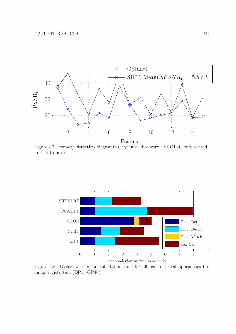
4.2 Test results . . . . . . . . . . . . . . . . . . . . . . . . . . . . . . . . . 52

4.2.1 Pair selection modi . . . . . . . . . . . . . . . . . . . . . . . . . 52

4.2.2 Feature-based approaches . . . . . . . . . . . . . . . . . . . . . 57

4.2.3 Comparison with intensity-based approach . . . . . . . . . . . . 60

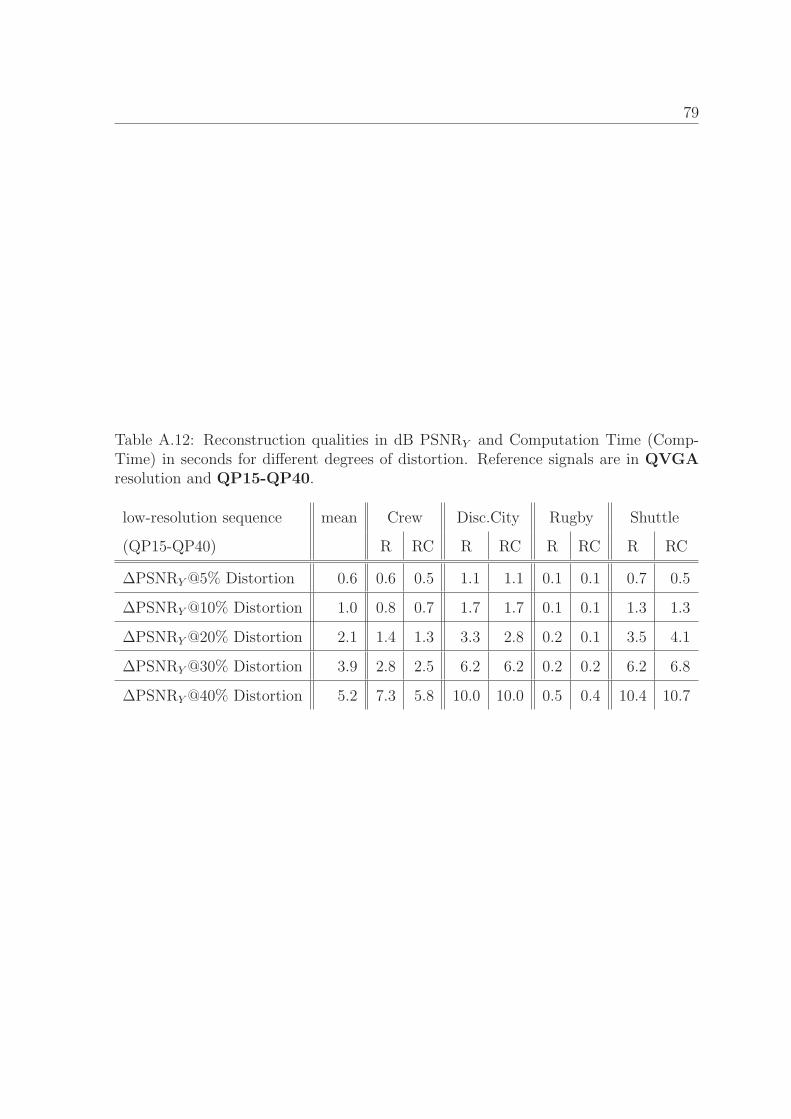
4.2.4 Performance depending on the degree of distortion . . . . . . . 61

4.2.5 Oracle-based measurements . . . . . . . . . . . . . . . . . . . . 63

5 Conclusion and Outlook 67

A Appendix 70

List of figures 83

List of tables 85

CONTENTS III

List of references 89

ABSTRACT V

Abstract

Mobile reception of digital TV signals such as DVB-T yields to block and slice losses

in TV images. In the future, mobile devices can deal with more than one digital TV

signal simultaneously. Inter-sequence error concealment conceals these errors by using

a reference signal such as a DVB-H or a T-DMB signal. After temporal synchroniza-

tion, the signals have to be registered spatially due to different image resolutions. Up

to now, a numerical approach is applied for image registration having a high com-

plexity. Feature-based approaches for image registration which can reduce the com-

plexity are evaluated regarding registration quality and computation time. Detailed

analysis in this work points out that the SIFT detector outperforms both the SURF

detector and the Harris-Laplace detector regarding sub-pixel accuracy. The SURF de-

scriptor achieves at least similar performance as SIFT, GLOH and PCA-SIFT by a

reduced complexity. Instead of taking the most certain pairs in the descriptor space, a

Speeded-Up-Search is introduced to select the best pairs in the image-space. Simulation

results show that the combination of the SIFT detector, the SURF descriptor and the

Speeded-Up-Search outperforms previous feature-based techniques for inter-sequence

error concealment regarding registration quality (on average by 0.2 dB PSNRY ) and

computational complexity (10%-15%). Furthermore, the simulations demonstrate that

the proposed algorithm for image registration yields to similar registration results as

the numerical approach for reference signals being compressed with high bitrates while

reducing the computation time by a factor of ten.

VI ZUSAMMENFASSUNG

Zusammenfassung

Der mobile Empfang digitaler TV-Signale, wie zum Beispiel DVB-T, kann zu Block-

oder Zeilenverlusten im dekodierten TV-Bild fuhren. Zukunftig werden mobile Gerate

gleichzeitig mehrere digitale TV Signale empfangen konnen. Die Inter-Sequenz-Fehler-

Verschleierung kann die auftretenden Verlustbereiche verschleiern - mit Hilfe eines Ref-

erenzsignals, beispielsweise mit einem DVB-H-Signal oder einem T-DMB-Signal. Nach-

dem die Signale zeitlich synchronisiert wurden, mussen sie ortlich registriert werden, da

die Signale unterschiedliche Bild-Auflosungen besitzen. Bisher steht fur diesen Zweck

ein numerisches Verfahren zur Verfugung, welches jedoch eine sehr hohe Rechenkom-

plexitat aufweist. Merkmalsbasierte Verfahren zur Bildregistrierung konnen diese Kom-

plexitat reduzieren. In dieser Arbeit werden diese Ansatze anhand ihrer Registrierungs-

qualitat und ihrer Rechenkomplexitat verglichen. Diese Arbeit macht deutlich, dass

der SIFT-Detektor die beiden anderen getesteten Detektoren SURF und Harris-Laplace

hinsichtlich der Subpixel-Genauigkeit deutlich ubertrifft. Obwohl der SURF-Deskriptor

die geringste Komplexitat aufweist, erreicht er mindestens die gleiche Leistungsfahigkeit

wie die Deskriptoren SIFT, GLOH und PCA-SIFT. Anstatt die Paare zu nehmen,

welche im Deskriptor-Raum die niedrigste Distanz aufweisen, wird ein Speeded-Up-

Search Verfahren vorgestellt, welches die besten Paare im Bildraum findet. Die Sim-

ulationsergebnisse zeigen, dass fur eine merkmalsbasierten Inter-Sequenz-Fehler-Ver-

schleierung eine Kombination aus SIFT-Detektor, SURF-Deskriptor und dem Speeded-

Up-Search-Verfahren am besten geeignet ist, da es die bisherigen merkmalsbasierte

Techniken sowohl bezuglich der Rekonstruktions-Qualitat (im Schnitt um 0.2 dB PSNRY )

als auch bezuglich der Rechenkapazitat (um 10% bis 15%) ubertrifft. Weiterhin zeigen

VII

die Simulationsergebnisse von Referenz-Sequenzen mit hohen Bitraten, dass der vorgeschla-

gene Algorithmus ahnliche Ergebnisse liefert wie das numerische Verfahren. Die Rechen-

zeit kann dabei jedoch um den Faktor zehn verringert werden.

VIII LIST OF ABBREVIATIONS

List of abbreviations

ATSC Advanced Television Systems Committee

BMA Boundary Matching Algorithm

CABLR Content-Based Adaptive Spatio-Temporal Method

CC Cross-Correlation

CIF Common Intermediate Format

CompTime Computational Time

CT Computed Tomography

DMVE Decoder Motion Vector Estimation

DOG Difference of Gaussian

DVB-C Digital Video Broadcasting - Cable

DVB-H Digital Video Broadcasting - Handheld

DVB-S Digital Video Broadcasting - Satellite

DVB-T Digital Video Broadcasting - Terrestrial

EBMA Extended Boundary Matching Algorithm

FBIR Feature-Based Image Registration

FSE Frequency Selective Extrapolation

GBM Gradient-Based Boundary Matching

GLOH Gradient Location and Orientation Histogram

HRI High-Resolution Image

IFS Improved Fading Scheme

II Integral Images

IX

ISDB Integrated Services Digital Broadcasting

IR Image Registration

ISEC Inter-Sequence Error Concealment

LESH Local Energy Shape Histogram

LO-RANSAC Local Optimized RANSAC

LRI Low-Resolution Image

LMA Levenberg-Marquardt algorithm

MI Mutual Information

MPEG Moving Picture Experts Group

MSE Mean Squared Error

M-SAC Estimation Sample Consensus

NMR Nuclear Magnetic Resonance

PCA Principle Components Analysis

PSNRY peak signal-to-noise ratio in the luminance

QP Quantization Parameter

QVGA Quarter Video Graphics Array

R resized

RC resized and cropped

RANSAC Random Sample Consensus

SBTFS Spatio-Bi-Temporal Fading Scheme

SIFT Scale-Invariant Feature Transform

SSDA Sequential Similarity Detection Algorithm

SSE Sum of Squared Errors

STBMA+PDE Combination of spatio-temporal boundary matching algo-

rithm and partial differential equation

SU Speeded-Up-Search

SURF Speeded-Up Robust Features

T-DMB Terrestrial - Digital Multimedia Broadcasting

U-SURF Upright SURF

X

FORMULA SYMBOLS XI

Formula symbols

∗ convolution

α angle of rotation deformation

κ number of pairs taken at refinement step

λ threshold used in RANSAC and M-SAC

λpenalty cost value for an outlier in M-SAC

µ(x, y, σI , σN ) second order moment matrix

µab entry of second order moment matrix at a,b

ω factor for refinement

ρ factor for refinement

σ standard deviation

σD standard deviation of the differentiation scale

σI standard deviation of the integration scale

σn standard deviation of the pre-defined scale

τ feature of matched feature pair

det(.) determinant of .

LoG(x, y, σ) Laplacian of Gaussian at scale σ at pixel position (x,y)

trace(.) trace of .

θ distance threshold

θ(x, y) orientation of gradient in location (x, y)

Aj,k candidate transformation matrix of pairs j and k

× times

XII

h′

i position vector of upscaled low resolution feature in high res-

olution image

hi position vector of feature in high resolution image

li position vector of feature in low resolution image

x vector consisting of σ and coordinates x and y

LRIup(m,n) value of pixel (m,n) in upscaled LRI

A transformation matrix

ALS matrix for least-squares algorithm

ai feature in image A

aij parameters for bicubic interpolation

bi feature in image B

c vector consisting of parameters c1 and c3

costFull(j) cost for pair j in full search

costRANSAC(j, k) cost in RANSAC using j and k for transformation

costMSAC(j, k) cost in MSAC using j and k for transformation

costSpeed(j) cost for pair j in Speeded-Up Search

cost(j, k) cost for the combination of j and k as keypoint set

coverness(x,y) coverness in pixel position (x, y)

ci parameter in transformation matrix

c parameter set in transformation matrix

ci parameter in candidate transformation matrix

d(i) distance of keypoint i for pair selection

di(j, k) distance of keypoint pair i using j and k for transformation

in RANSAC

dMSAC,i(j, k) distance of keypoint pair i using j and k for transformation

in M-SAC

Dxy box filter which approximates derivatives in x and y direction

desc(ai) descriptor vector of ai

det(·) determinant of ·

FORMULA SYMBOLS XIII

det(Happrox) determinant of the approximated Hessian matrix

dis(ai, bj) distance between descriptors ai and bj

disti(A) distance in image-space between h′

i and hi

DOG(x, y, σ) Difference of Gaussian

E(·) expected value of ·eISEC minimum of all tested MSE

f ratio beween the largest magnitude eigenvalue and the small-

est one

G(σ) Gaussian function

G(σI) Gaussian function with standard deviation σI

G(x, y, σ) Gaussian function

H(X) entropy of random variable X

H(x, y, σ) Hessian matrix

HRI(m,n) value of pixel (m,n) in HRI

I number of features found in image A

IΣ(x, y) entry of integral image at location (x, y)

Im(x, y) Image value at location (x, y)

J number of features found in image B

L(x, y, σ) Gaussian image

Lx(x, y, σD) derivative of pixel position (x,y) at scale σD in x direction

Lxy entry at location (x, y) of the convolution of the Image with

Gaussian second order derivative in x and y direction

LRI(m,n) value of pixel (m,n) in LRI

m vector consisting of m-components of all taken pairs

m coordinate of width in high resolution image

M width of high resolution image

m(x, y) gradient magnitude at location (x, y)

mi coordinate of width of feature i in high resolution image

m′

i coordinate of width of the upscaled low resolution feature i

XIV

MSE mean squared error

n coordinate of height in high resolution image

N height of high resolution image

NR number of runs for a pair selection technique

ni coordinate of height of feature i in high resolution image

n′

i coordinate of width of the upscaled low resolution feature i

pij pixel value at location (i− 1; j − 1)

P number of pairs after refinement step

P (X) probability distribution of random variable X

Q number of equations for least-squares algorithm

qcFull(i, j) quality criterion in full search using i and j for transformation

qcSpeed(i, j) quality criterion in Speeded-Up Search using i and j for trans-

formation

r coordinate of width in low resolution image

R width of low resolution image

ri coordinate of width of feature i in low resolution image

s coordinate of height in low resolution image

S height of low resolution image

si coordinate of height of feature i in low resolution image

SSE Sum of Squared Errors

t time

tr(·) trace of ·W (m,n) binary matrix

MI mutual information

CHAPTER 1. INTRODUCTION 1

Chapter 1

Introduction

Nowadays Digital Video Broadcasting - Terrestrial (DVB-T) is the most popular stan-

dard in several countries. It is used in Europe, Russia, India, Australia and some

countries in Asia and Africa. Most of the other countries use equivalent standards for

digital TV such as Advanced Television Systems Committee (ATSC) in North America

and Integrated Services Digital Broadcasting (ISDB) in Japan. DVB-T provides high

video quality using mostly the MPEG-2 codec. MPEG-4 is less available such as in

Slovenia. MPEG-4 is gaining fast popularity and is becoming more and more interest-

ing for the other countries.

DVB-T is designed for both stationary and portable TV reception. Using DVB-T for

mobile reception can be difficult. The quality of reception depends on the channel

properties. Due to the Doppler effect, the carrier frequency shifts when the receiver

moves relatively to the broadcast station. Furthermore, signal reflection and shadow-

ing change more quickly. If the broadcast station has a large distance to the receiver,

the signal strength is very weak. As a result, sometimes the signal cannot be detected

properly and after demodulation, some bits may be detected incorrectly. Due to the

usage of block-based video codec in MPEG-2 and bad channel characteristics, block or

slice losses in the decoded image can occur.

One way to conceal these errors is to examine the neighborhood of the erroneous area

in the image or the frame before and/or after the erroneous one. They are also called

2

Figure 1.1: Multi-Broadcast Receiver [1]

intra-sequence concealment technique (more details in section 2.1). However, the qual-

ity of error concealment can be enhanced even further to provide better TV reception

for the customer.

In Europe especially the Terrestrial - Digital Multimedia Broadcasting (T-DMB) and

Digital Video Broadcasting - Handheld (DVB-H) signals are transmitted terrestrial in

addition to DVB-T. The video quality of these three signals differs not only in reso-

lution, but also in higher compression rate. Since T-DMB and DVB-H are designed

for mobile reception, they have more sophisticated schemes for channel coding which

provides error-free reception. All these characteristics yield to a bitrate of around 300

kbit/s for a TV station with DVB-H having QVGA (Quarter Video Graphics Array)

resolution and in average 3 to 5 Mbit/s for a TV station with DVB-T.

For mobile scenarios it is possible to gain a TV signal combining the high video quality

of DVB-T with error protection or concealment techniques.

In the future Multi-Broadcast-Receivers will be available that can receive more than

one TV signal. It is obvious that this redundancy can be used to get a diversity gain.

Inter-Sequence Error Concealment (ISEC), which is described in section 2.2, is a way

to profit from this Multi-Broadcast-Receiver. It conceals the distorted area in a DVB-T

CHAPTER 1. INTRODUCTION 3

Figure 1.2: Mobile Multi-Broadcast Reception [1]

frame by using one or more reference sequences which have the same image content.

Remaining errors can be concealed by using another DVB-T signal as reference with

the same channel coding technique. The two or more signals have the same resolution

and no synchronization for the image transformation is necessary.

Since DVB-H and T-DMB signals can be assumed to be error-free also for mobile re-

ception, they are a good alternative to be used as reference signals for ISEC. Their

resolutions are a major disadvantage: T-DMB deals with QVGA (320x240) resolu-

tion, DVB-H with QVGA and CIF (Common Intermediate Format) (352x288) as well.

Since the content is the same, shown in [2], it outperforms the intra-sequence error

concealment approaches, even for low bitrates.

DVB-T signals have different resolution (720x576) and possibly different aspect ratios

than these signals, so the images of the two or more sequences have to be registered for

ISEC. The Image Registration (IR) is described in section 3. In this step, the trans-

formation correspondences are determined. The goal is to find a registration approach

which delivers accurate transformation parameters while having a low computational

complexity. The latter claim is important because ISEC shall perform in mobile scenar-

ios like in-car TV reception where computation power, battery life and battery power

are limited.

One way to perform image registration for ISEC is to use Area-Based Image Registra-

tion. Several approaches are introduced in section 3.1 including the method which is

used for ISEC. Feature-Based Image Registration (FBIR) approaches are interesting

for ISEC as they reduce the complexity of ISEC. These methods are described in sec-

4

tion 3.2. Scale-Invariant Feature Transform (SIFT) [3] is a particular FBIR approach

that already works well with ISEC[4]. The emphasis of this work will be the testing

of FBIR methods using T-DMB or DVB-H signals as reference because up to now the

performance of FBIR regarding ISEC is nearly unknown. Section 3.2 also describes

how the features are used for ISEC. This comprises the way feature points are deter-

mined, described, matched and how the best performing feature points are selected.

The chosen parameter set fulfilling the best performance and the simulation results are

explained in section 4.

Until now, only terrestrial TV standards have been mentioned. Of course, other sig-

nals such as DVB-S as satellite and DVB-C as cable reception standards are possible

for ISEC. However, the main focus of ISEC is on mobile reception, so using cable is

impossible and readjusting the satellite antenna while moving is also a very ambitious

challenge. Thus, these scenarios are not part of this project.

Further enhancement will be gained by using more than one reference signal. A good

combination can be for instance DVB-T and DVB-H: Most of the block or slice losses

are then concealed error-free by the DVB-T signal. The rest of distortion is finally

concealed by the DVB-H signal. This combination is not tested in this project because

the additional gain is obvious and can be calculated easily.

CHAPTER 2. ERROR CONCEALMENT 5

Chapter 2

Error Concealment

In this section two important ways to conceal error in a digital TV signal are described

in detail. In section 2.1 temporal, spatial and spatio-temporal error concealment ap-

proaches are introduced. They use either the neighborhood in the erroneous frame or

the previous and following frames or both to estimate the missing blocks. To increase

the performance of error concealment even further, the inter-sequence error conceal-

ment can be applied (see section 2.2). The positions of the erroneous pixels are known

at the decoder because the used channel coding can identify parts of the bitstream

which are defective.

2.1 Recent Error Concealment Techniques

Without any reference signals several temporal, spatial or spatio-temporal error con-

cealment techniques are available.

The Boundary Matching Algorithm (BMA), the Extended Boundary Matching Algo-

rithm (EBMA) [5] and the Decoder Motion Vector Estimation (DMVE) [6] are three

important temporal error concealment approaches. BMA reconstructs lost motion vec-

tor by minimizing the edges which appear during reconstruction. EBMA reconstructs

lost prediction errors in addition. DMVE maximizes the similarity between neighbor-

ing and candidate blocks.

6

Two state-of-the-art spatial error concealment techniques are the Frequency Selective

Extrapolation (FSE) [7] and the Bilinear Interpolation, also known as H264.Intra [8].

The first algorithm takes surrounding image sample to estimate the spatial frequency

spectrum of the lost block. The latter one interpolates adjacents error-free pixels.

Further advancement can be achieved by combining spatial and temporal techniques.

These approaches are called spatial-temporal methods. Content-Based Adaptive Spatio-

Temporal Method (CABLR) [9], Spatio-Bi-Temporal Fading Scheme (SBTFS) [10], Im-

proved Fading Scheme (IFS) [11], Gradient-Based Boundary Matching (GBM) [12] or

a combination of spatio-temporal boundary matching algorithm and partial differential

equation (STBMA+PDE) [13] are some well performing methods. The spatial part of

CABLR replaces erroneous pixels using surrounding neighborhood edge information

and structure. The temporal part estimates the lost motion vector with an adaptive

temporal correlation method. SBTFS estimates a lost macro block pixel-wise spatially

and/or bi-temporally from the previous and the future frame. IFS works with hybrid

approaches using adaptive weights. GBM includes a mode selection algorithm which

decides whether to take the temporal or spatial algorithm or both to estimate the lost

macroblock. STBMA+PDE consists of two stages: In the first step a cost function

is minimized to find a reference macroblock which conceals the error. It covers both

spatial and temporal methods. In the second step this result is refined further using

the gradient field of the reconstructed block.

Troger [2] tested BMA, H.264 Intra and DMVE in the field of error concealment of

distorted DVB-T signals. He found out that in general BMA performs worse and that

DMVE performs best in almost all tested sequences. In some cases H.264 Intra has the

best performance regarding the calculated peak signal-to-noise ratio (PSNRY ) value of

the luminance.

But all these error concealment techniques have limited performance. Objective as well

as subjective measures show that it has to be enhanced further more.

2.2. INTER-SEQUENCE ERROR CONCEALMENT 7

2.2 Inter-Sequence Error Concealment

This section describes the specific steps in ISEC in more detail. It considers the signals

obtained by the multi-broadcast-receiver mentioned in section one.

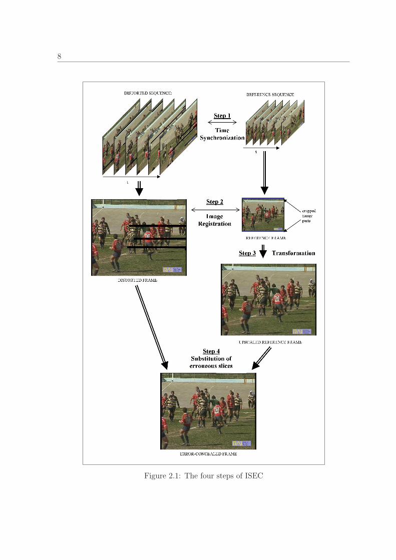
In Fig. 2.1 the four steps of ISEC are visualized and explained in the following:

First, the different signals have to be synchronized in time. A delay between these

signals appears because they use different channel coding and source coding and so

the processing time varies. In addition, the transmission runtimes differ since the

distances to different senders are not equal. Furthermore, the senders might not be

synchronized.

Troger [14] shows a method to synchronize video signals with different resolutions

by using a numerical optimization technique. This approach is robust against image

cropping, different compression rates and block or slice losses. In [15] a simpler method

is introduced to show what happens when the reference signal has the same resolution

as the original signal. The mean squared error of error-free parts in the images over

time is minimized.

Step two covers image registration between the time-synchronized frames. The only

goal of step two is to obtain the transformation matrix in order to transform the Low-

Resolution Image (LRI) into the resolution of the erroneous High-Resolution Image

(HRI). In a way the LRI can be seen as a HRI, which was cropped, downscaled and

further compressed at the sender. Since a constant transformation is not part of the

standard, the inverse-transformation has to be identified for each reference signal to

perform ISEC. Cropping and resizing can be characterized as non-uniform scaling and

translation. These are linear transformations which can be described by an affine 3-

by-3 transformation matrix (see Eq. (2.1)).

The HRI has the resolution M × N, the LRI has the resolution R × S. The pixel

positions in the HRI are defined as m ∈ {1, . . . ,M} and n ∈ {1, . . . , N}, the same

declaration is applied for the LRI with r ∈ {1, . . . , R} and s ∈ {1, . . . , S}. The mapping

between HRI and LRI can be characterized with:

8

Figure 2.1: The four steps of ISEC

2.2. INTER-SEQUENCE ERROR CONCEALMENT 9

Figure 2.2: Translation and Scaling

m

n

1

=

c1 0 c3

0 c5 c6

0 0 1

r

s

1

(2.1)

These four parameters c1, c3, c5 and c6 have to be determined [14].

Moreover, the approach to find these parameters has to be robust to lost image infor-

mation like block losses. The image registration itself is discussed in detail in section

three.

After the four parameters of the transformation matrix are computed, the LRI can be

transformed into the higher resolution in step three.

After the first three steps, at least two signals with the same content and the same

resolution are available. If the reference signal is upsampled, this image will have

lower image quality as the LRI was already compressed and the interpolation in step

three results in less quality compared to the HRI. Furthermore, potentially cropped

image parts in the LRI cannot be reconstructed during the upsampling process. These

changeless missing blocks have to be reconstructed with intra-sequence error conceal-

ment methods (see section 2.1).

In the following sections, this thesis will emphasize on step two of ISEC. The sequences

are assumed to be time-synchronized.

10 CHAPTER 3. IMAGE REGISTRATION

Chapter 3

Image Registration

First, this section describes the image registration in general. Secondly, the area-based

image registration is introduced. A numerical intensity-based approach, as an example

of area-based image registration, is used in ISEC. It is described in detail in section

3.2.2. The focus of this thesis is shown in the third section 3.3.

3.1 Overview

As an accurate transformation is indispensable, image registration is a crucial part in

ISEC. The domain of image registration is extensive. In the 90’s over 1000 papers were

published covering this field of application. The publication of Barbara Zitova et al.

[16] gives a very good overview on this topic. In the following the classifications of

image registration algorithms by Zitova will be explained.

The combination of various image data gained by IR is used to achieve additional in-

formation. Zitova classifies IR into area-based and feature-based methods. Area-based

techniques are also called intensity-based or pixel-based in the literature. To stay

consistent with Zitova’s notation area-based is used in the following sections. Both

methods, area-based and feature based algorithms, are described in more detail in

section 3.1 and 3.2. Later, this work will focus on the performance of feature-based

methods in context of ISEC.

3.1. OVERVIEW 11

Figure 3.1: Image registration of two images

Another classification is done concerning the available image data set: The images can

be registered being acquired at different viewpoints (multiview analysis), at different

times (multitemporal analysis) and with different sensors (multimodal analysis). Then

the so called scene-to-model registration is also possible.

Furthermore it is possible, that the images may have a variety of degradations like ge-

ometric or radiometric deformations. Szeliski [17] gives a good overview of the possible

deformations. They are shown in Fig. 3.2 with the corresponding Eq. (3.1) - (3.4).

The deformation in ISEC was already described in Fig. 2.2 and Eq. (2.1).

Translation can be described with

m

n

1

=

1 0 c3

0 1 c6

0 0 1

r

s

1

, (3.1)

rotation can be described with

12

(a)

(b)

(c)

(d)

Figure 3.2: Deformations: a) Translation b) Rotation c) Affine d) Perspective

3.1. OVERVIEW 13

m

n

1

=

cosα − sinα 0

sinα cosα 0

0 0 1

r

s

1

, (3.2)

affine deformations can be described with

m

n

1

=

c1 c2 c3

c4 c5 c6

0 0 1

r

s

1

, (3.3)

and perspective deformations can be described with

m

n

1

=

c1 c2 c3

c4 c5 c6

c7 c8 c9

r

s

1

. (3.4)

In addition to these deformations, noise, contrast and illumination corruption also ap-

pear, as well as compression effects.

The importance of IR can be seen on the various applications used. It is used for remote

sensing, like weather forecast, image mosaicing, change detection, environmental mon-

itoring and multispectral classification for instance. In medicine, it is used to combine

Computer Tomography (CT) and Nuclear Magnetic Resonance (NMR) data and the

monitoring of tumor growth and treatment. Two further applications are cartography

and Computer Vision. Of course, this list is not complete but shows how multifaceted

is this research field. It is obvious that every single IR algorithm performs differently

in each application regarding complexity cost and accuracy of the registration.

Zitova groups all IR approaches into 4 steps. The first step is the feature detection,

which is mainly important for feature-based methods. Salient and possibly distinc-

tive objects like lines, edges, corners or line intersections are detected and described

by a representation vector, which is called descriptor. After that, the features are

14

matched according to these descriptors in the second step. With alignment between

the sensed and reference images, the mapping functions are calculated using these cor-

respondences. Zitove integrates this calculation in the third step. Image Resampling

and Image Transformation are included in the last step. The transformation can be

performed using the means of the mapping functions. Non-integer pixel values are

calculated with interpolation methods such as nearest-neighbor interpolation, bilinear

interpolation or bi-cubic interpolation.

The requirements of a powerful IR algorithm are described below. The features should

be distinctive and spread over the whole space of the images. Furthermore, they should

be easy to detect and should have common elements in all images, including the case

of object occlusion on an image. To gain accurate mapping parameters, features have

to be localized more accurately. Robustness to image degradations and deformations

often is also very crucial. Ideal, robustly and accurately features are detected in all

projections regardless of particular image deformations.

The matching step as the last one should also perform robust and efficient. Discarding

features without counterparts avoids degrading the accuracy of the mapping functions.

If the rate of deformation is known a-priori, this can be used in the third step of IR.

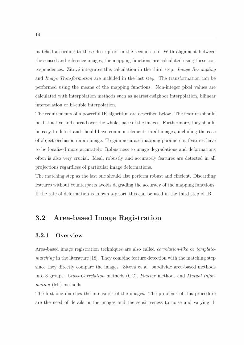
3.2 Area-based Image Registration

3.2.1 Overview

Area-based image registration techniques are also called correlation-like or template-

matching in the literature [18]. They combine feature detection with the matching step

since they directly compare the images. Zitova et al. subdivide area-based methods

into 3 groups: Cross-Correlation methods (CC), Fourier methods and Mutual Infor-

mation (MI) methods.

The first one matches the intensities of the images. The problems of this procedure

are the need of details in the images and the sensitiveness to noise and varying il-

3.2. AREA-BASED IMAGE REGISTRATION 15

lumination. Modifications by [19] cover also affine differences between images, but

the computational demands rise with the degree of deformation. Object Recognition

[20, 21] is another extension of CC which is based on increment sign correlation. Se-

quential Similarity Detection Algorithm (SSDA) is a way to speed-up the procedure by

using thresholding.

Pratt [22], Anuta [23] and Van Wie et al. [24] propose preprocessings before executing

the CC. Pratt filters the image before applying the CC to gain robustness to noise or

highly correlated images. Anuta and Van Wie published an edge-based correlation.

Since this algorithm works only on the edges of the images, it is more robust against

intensity varations between the images. Huttenlocher [25] first computes binary images

and then registeres the images by means of the Hausdorff distance. This registration

method covers translation and rotation transformations. Since there has been a lot of

research in the field of CC, a lot of fast implementations are available.

The second group of area-based methods is the Fourier. Compared to the CC, it has

less computational demands. If the images are distorted with frequency-dependent

noise, it performs very well as it works in the frequency domain. The Fourier methods

consist of phase correlation in which, first the Cross-Power-Spectrum of the sensed and

the reference images is calculated [26] and then the maxima in its inverse are detected.

Fourier approaches perform fast, even for large images and are less sensitive to illumi-

nation changes. Further extensions of the phase correlation techniques are invariant to

rotation [27] and to scaling [28, 29, 30]. Totally affine invariance is introduced in [31].

Last but not least, the most recent area-based technique is the MI method. In health

care applications it bears a high meaning. The MI measures the statistical similarities

between two data. The MI between two Random Variables X and Y can be described

with Eq. (3.5). H is the entropy, calculated with H(X) = −E{log(P (X))}. P(X) is

the probability distribution of X [16].

MI(X, Y ) = H(Y )−H(Y |X) = H(X) +H(Y )−H(X, Y ) (3.5)

16

The goal is to maximize the MI. Viola and Wells [32] use gradient descent optimization,

Thevenaz and Unser [33, 34, 35] use the Levenberg-Marquardt algorithm (LMA) [33]

the maximization application. Another way is shown in [36] where the Gauss-Newton

numerical minimization algorithm is utilized to minimize the sum of squared differences.

The latter approach and the LMA are both based on numerical optimizations. A lot

more approaches and ideas for MI can be found in the literature.

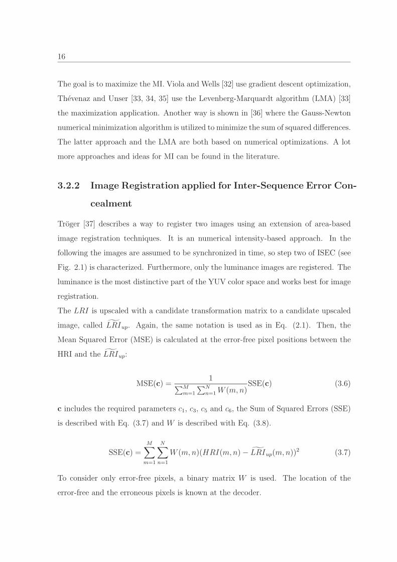
3.2.2 Image Registration applied for Inter-Sequence Error Con-

cealment

Troger [37] describes a way to register two images using an extension of area-based

image registration techniques. It is an numerical intensity-based approach. In the

following the images are assumed to be synchronized in time, so step two of ISEC (see

Fig. 2.1) is characterized. Furthermore, only the luminance images are registered. The

luminance is the most distinctive part of the YUV color space and works best for image

registration.

The LRI is upscaled with a candidate transformation matrix to a candidate upscaled

image, called LRIup. Again, the same notation is used as in Eq. (2.1). Then, the

Mean Squared Error (MSE) is calculated at the error-free pixel positions between the

HRI and the LRIup:

MSE(c) =1

∑Mm=1

∑Nn=1 W (m,n)

SSE(c) (3.6)

c includes the required parameters c1, c3, c5 and c6, the Sum of Squared Errors (SSE)

is described with Eq. (3.7) and W is described with Eq. (3.8).

SSE(c) =M∑

m=1

N∑

n=1

W (m,n)(HRI(m,n)− LRIup(m,n))2 (3.7)

To consider only error-free pixels, a binary matrix W is used. The location of the

error-free and the erroneous pixels is known at the decoder.

3.3. FEATURE-BASED IMAGE REGISTRATION 17

W (m,n) =

1 if HRI(m,n) is error-free

0 else

(3.8)

The goal is to find the 4 parameters which minimize the MSE. The MSE is determined

over the time t by:

eISEC = minc∈R4

(MSE(c, t)) (3.9)

The LMA as a robust gradient descent approach is applied to minimize all candidate

vectors c (Eq. (3.9)). The way LMA is applied for ISEC is described in detail in [2].

3.3 Feature-based Image Registration

The second main classification in image registration theory is the feature-based image

registration. Instead of matching the whole image with other images, the FBIR searches

for distinguish and characteristic points on the images to build the correspondences.

These points are called features.

Section 3.2 is split into the 6 steps of FBIR: Feature Detection, Feature Description,

Feature Matching, Pair Refinement, Pair Selection and Image Transformation (see Fig.

3.3).

3.3.1 Feature Detection

Features are also called interest points or salient points in the literature [17]. From sec-

tion 3.3.5 on, they are named keypoint, because the algorithm then only operates with

the pixel-position of each feature. The features have to be distinct and spread all over

the image. A robust feature-based approach detects a high number of common features

in the two images. The positions of the features should be stable. Furthermore, their

detection and description has to be invariant to several kinds of deformations and has

18

Figure 3.3: Feature-Based Image Registration of Low-Resolution Image (LRI) andHigh-Resolution Image (HRI)


to be robust against illumination and contrast variations, noise and compression.

Zitova [16] also gives an extended overview of methods for feature detection. She

groups them into region, line and point features.

Regions are closed-boundary areas with high contrast of appropriate size in the image

like lakes, buildings or shadows. Subpixel accuracy can be achieved by using segmen-

tation [38], scale invariance by using virtual circles and distance transform [39], and

affine invariance by Harris corner detector [40].

The second group includes edge detector like the Canny detector [41] or the Laplacian

of Gaussian [42]. Zohlanicet et al. [43] register line segments.

Points are usually intersections or corners in the image. Points can be found by Gabor

wavelets [44, 45] or local extrema in wavelet transforms [46, 47]. Kitchen and Rosenfeld

[48] describe a way to use the second order partial derivatives for detecting features.

Local extrema of Gaussian curvatures are performed for this application in [49]. A rise

of computational complexity on the one hand and a rise of robustness on the other

hand is reached by using the first order derivative in [50].

Szeliski [17] found out that the reliability of motion estimates depends on the smallest

eigenvalue λ0 of the image Hessian matrix. Harris and Stephens [51] use the Hessian

and the eigenvalue images to detect features. They also introduced a simpler method

which takes the determinant and the trace of the processed Hessian Matrix. Brown et

al. [52] uses the harmonic mean det(A)tr(A)

of the Hessian. In section 3.3.1.1, the usage of

the Difference of Gaussian (DOG) instead of the Laplacian of Gaussian is described

more in detail. A further acceleration in the detection step is explained in section

3.3.1.2, where an approximation of the determinant of the Hessian is used. The scale-

normalized Laplacian operator [53] was developed further by Mikolajczyk et al. [54]

to the Harris-Laplacian (see section 3.3.1.3). They all work with image-pyramides to

detect the features in scale-space (see Fig. 3.8).

20

Figure 3.4: Creation of the DOGs [3]

3.3.1.1 SIFT Detector

The SIFT detector [3] consists of cascade filtering to reduce the computional cost.

First, candidate locations are found and then further refined in a second step. Lastly

a main orientation is assigned to each keypoint.

The main component of SIFT is the detection of features in the scale-space. The

Gaussian function G(x, y, σ) is one scale-space kernel. L(x, y, σ) is the convolution of

this Gaussian function with an image Im(x, y).

G(x, y, σ) =1√2πσ2

e−(x2+y2)/2σ2

(3.10)

L(x, y, σ) = G(x, y, kσ) ∗ Im(x, y) (3.11)


Scale invariance is achieved by the normalized Laplacian which is equal to the deriva-

tive of the Gaussian. So, the Difference of Gaussian is a close approximation to the

Laplacian.

∂G

∂σ= σ∇2G (3.12)

Lowe searches for scale-space extrema in the convolution of the Difference of Gaussian

function with the image Im(x, y) to detect keypoint candidates:

DOG(x, y, σ) = (G(x, y, kσ)−G(x, y, σ)) ∗ Im(x, y) (3.13)

= L(x, y, kσ)− L(x, y, σ)

The scale space is divided into octaves [55]. One octave consists of a series of filter

responses which is obtained by convolving the same image with a filter of increasing

size. An octave encompasses a scaling factor of 2 and is further subdivided into scale-

levels.

In SIFT, the image is incrementally convolved with the Gaussian kernel for each octave

in the scale space. Then adjacent Gaussian images are substracted to get the DOG

(see Eq. (3.13)). For the next octave, all Gaussian images are downsampled by a factor

of two and the DOG are obtained in the same way (see Fig. 3.4).

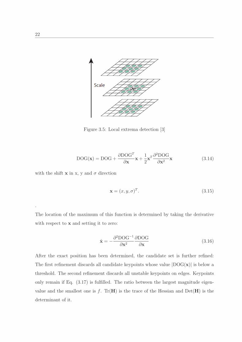
After the DOGs have been calculated, the local extrema have to be detected. Each

sample point in the DOG images is compared to its eight neighbors in the current

image and its nine neighbors in the images one scale above and below. If the sample

point has the maximum value of 27 points, it becomes a candidate keypoint (see Fig.

3.5).

The exact scale and location of these extrema are calculated according to Braun [3].

He fits a 3D quadratic function to the candidate keypoint to find the interpolated

maximum in Eq. (3.14):

22

Figure 3.5: Local extrema detection [3]

DOG(x) = DOG+∂DOGT

∂xx+

1

2xT ∂

2DOG

∂x2x (3.14)

with the shift x in x, y and σ direction

x = (x, y, σ)T . (3.15)

.

The location of the maximum of this function is determined by taking the derivative

with respect to x and setting it to zero:

x = −∂2DOG−1

∂x2

∂DOG

∂x(3.16)

After the exact position has been determined, the candidate set is further refined:

The first refinement discards all candidate keypoints whose value |DOG(x)| is below a

threshold. The second refinement discards all unstable keypoints on edges. Keypoints

only remain if Eq. (3.17) is fulfilled. The ratio between the largest magnitude eigen-

value and the smallest one is f . Tr(H) is the trace of the Hessian and Det(H) is the

determinant of it.


Tr(H)2

Det(H)≤ (r + 1)2

r(3.17)

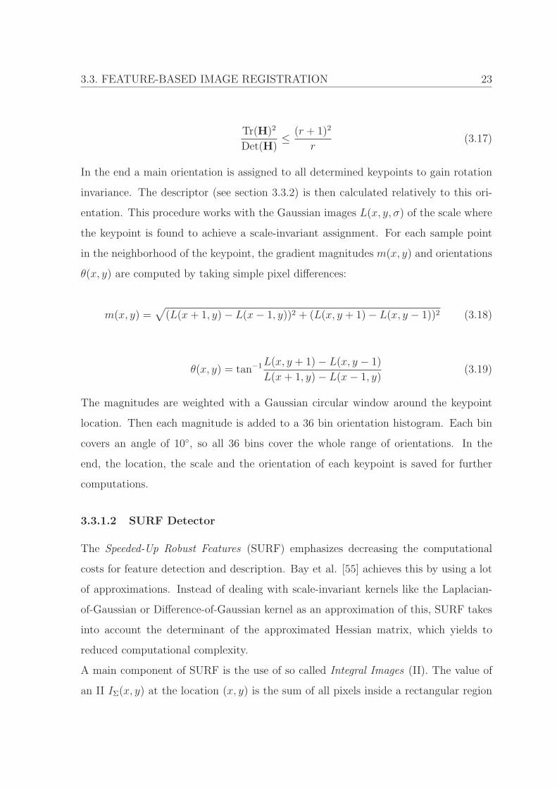
In the end a main orientation is assigned to all determined keypoints to gain rotation

invariance. The descriptor (see section 3.3.2) is then calculated relatively to this ori-

entation. This procedure works with the Gaussian images L(x, y, σ) of the scale where

the keypoint is found to achieve a scale-invariant assignment. For each sample point

in the neighborhood of the keypoint, the gradient magnitudes m(x, y) and orientations

θ(x, y) are computed by taking simple pixel differences:

m(x, y) =√(L(x+ 1, y)− L(x− 1, y))2 + (L(x, y + 1)− L(x, y − 1))2 (3.18)

θ(x, y) = tan−1L(x, y + 1)− L(x, y − 1)

L(x+ 1, y)− L(x− 1, y)(3.19)

The magnitudes are weighted with a Gaussian circular window around the keypoint

location. Then each magnitude is added to a 36 bin orientation histogram. Each bin

covers an angle of 10◦, so all 36 bins cover the whole range of orientations. In the

end, the location, the scale and the orientation of each keypoint is saved for further

computations.

3.3.1.2 SURF Detector

The Speeded-Up Robust Features (SURF) emphasizes decreasing the computational

costs for feature detection and description. Bay et al. [55] achieves this by using a lot

of approximations. Instead of dealing with scale-invariant kernels like the Laplacian-

of-Gaussian or Difference-of-Gaussian kernel as an approximation of this, SURF takes

into account the determinant of the approximated Hessian matrix, which yields to

reduced computational complexity.

A main component of SURF is the use of so called Integral Images (II). The value of

an II IΣ(x, y) at the location (x, y) is the sum of all pixels inside a rectangular region

24

Figure 3.6: Calculation of an Integral Image: Σ = A+D − (C + B)

from the origin to the location (x, y):

IΣ(x, y) =x∑

m=0

y∑

n=0

Im(m,n) (3.20)

Then, integrals over upright rectangular regions in the image Im can be easily calculated

by simple image additions and subtractions:

Keypoint candidates can be found with an approximation of the Hessian Matrix. The

image Im(x,y) is convolved with the four Gaussian second order derivatives:

Lxx(x, y, σ) =∂2

∂x2G(σ) ∗ Im(x, y) (3.21)

Lxy(x, y, σ) =∂2

∂x∂yG(σ) ∗ Im(x, y)

Lyx(x, y, σ) =∂2

∂y∂xG(σ) ∗ Im(x, y)

Lyy(x, y, σ) =∂2

∂y2G(σ) ∗ Im(x, y)

The Hessian matrix consists of these four derivatives.


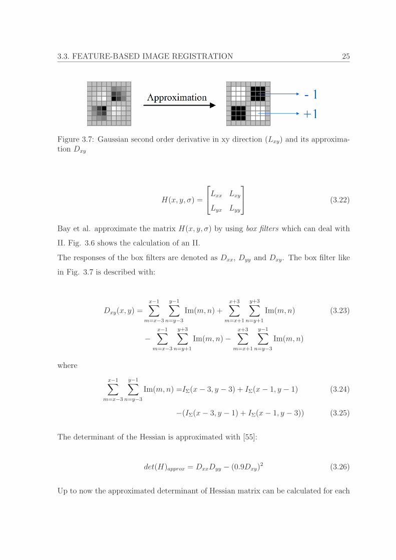
Figure 3.7: Gaussian second order derivative in xy direction (Lxy) and its approxima-tion Dxy

H(x, y, σ) =

Lxx Lxy

Lyx Lyy

(3.22)

Bay et al. approximate the matrix H(x, y, σ) by using box filters which can deal with

II. Fig. 3.6 shows the calculation of an II.

The responses of the box filters are denoted as Dxx, Dyy and Dxy. The box filter like

in Fig. 3.7 is described with:

Dxy(x, y) =x−1∑

m=x−3

y−1∑

n=y−3

Im(m,n) +x+3∑

m=x+1

y+3∑

n=y+1

Im(m,n) (3.23)

−x−1∑

m=x−3

y+3∑

n=y+1

Im(m,n)−x+3∑

m=x+1

y−1∑

n=y−3

Im(m,n)

where

x−1∑

m=x−3

y−1∑

n=y−3

Im(m,n) =IΣ(x− 3, y − 3) + IΣ(x− 1, y − 1) (3.24)

−(IΣ(x− 3, y − 1) + IΣ(x− 1, y − 3)) (3.25)

The determinant of the Hessian is approximated with [55]:

det(H)approx = DxxDyy − (0.9Dxy)2 (3.26)

Up to now the approximated determinant of Hessian matrix can be calculated for each

26

Figure 3.8: Building the scale-space. Left: filter size constant, image size varies; Right:filter size varies, image size constant [55]

pixel in image. The claimed scale-invariance is achieved by the following:

Instead of iteratively downsampling the image, only the box filters are changed in size

(see Fig. 3.8). Due to use of II the computational cost is very low.

Since box filters have integer size, there are not arbitrarily many scales to be proceeded.

The candidate keypoints are then obtained by taking the local maximum value within

a 3× 3× 3 neighborhood, like in SIFT technique (see Fig. 3.5).

The sub-pixel accuracy of these candidate keypoints has to be determined in the next

step. As in SIFT, also in SURF a 3D quadratic function is taken to interpolate pixel

position and scale. The Hessian matrix H can then be described with [56]:

H(x) ≈ H+∂HT

∂xx+

1

2xT ∂

2H

∂x2x (3.27)

Again, the location of the maximum of this function is determined by taking the

derivative with respect to x and setting it to zero:

x = −∂2H−1

∂x2

∂H

∂x(3.28)


3.3.1.3 Harris-Laplace Detector

The Harris-Laplace detector [57] combines the affine-invariant Harris–detector with the

Laplacian-based scale selection. The Harris detector is based on the second moment

matrix µ(x, y, σI , σn) where σI is the integration scale. σD is the differentiation scale

and Lx is the derivative in x direction. G(σI) is the Gaussian kernel with standard

deviation σI .

µ(x, y, σI , σn) =

µ11 µ12

µ21 µ22

(3.29)

= σ2DG(σI) ·

Lxx(x, y, σD) LxLy(x, y, σD)

LxLy(x, y, σD) Lyy(x, y, σD)

Then the trace and the determinant of the second moment matrix are taken to build

the coverness in each pixel position (x, y):

coverness = det(µ(x, y, σI , σD))− α · (trace(µ(x, y, σI , σD)))2 (3.30)

The demanded scale-space representation is computed with pre-defined scales σn =

1, 4n · σ0. Thus candidate keypoints are detected on each scale at local maxima in the

3 × 3 pixel neighborhood of the interest point. Unstable candidates are discarded by

thresholding the coverness.

The second stage of the Harris-Laplacian detector is the Laplacian scale selection. It

is an iterative approach to increase the keypoint’s precision in scale. A more exact

sub-pixel and scale accuracy is gained at the maximum of the Laplacian-of-Gaussian

function (3.31).

|LoG(x, y, σn)| = σ2n |Lxx(x, y, σn) + Lyy(x, y, σn)| (3.31)

28

3.3.2 Feature Description

The easiest way to describe a feature is to express it by its center of gravity [17]. A line

can be characterized by its ends and/or middle points. Again, Zitova [16] lists a lot

approaches for feature description. In the following I will focus on the most important

ones. Mostly features are described by their neighborhood. As in the area-based reg-

istration methods, cross-correlation and mutual information can be performed. There

are also some moment-based and moment invariant descriptors. Moreover, circular

moments, geometic orientations, angle differences, ellipticity and thinness are used to

build the descriptor. Generelly, the performance of a descriptor depends on the degree

of deformation.

Since the approaches search for features in the whole image area, translation is covered

anyway. Rotation-invariance is gained by assigning a dominant orientation for each

feature and a descriptor computation relative to this orientation. Brown et al. [52]

take the direction of the average gradient orientation of the direct neighborhood. In

SIFT (see section 3.3.2.1) and GLOH (Gradient Location and Orientation Histogram)

(see section 3.3.2.4) [54] the peak in the local gradient orientation histogram yields

to the dominate orientation. Scale-invariance can be achieved by working with local

maxima in the scale-space. Affine-invariance is performed differently. GLOH takes the

second moment matrix, Hager and Corso [58] use 2D oriented Gaussian kernels and

Freeman and Adelson [59] use steerable filter, which is a combination of derivatives of

Gaussian filters to detect edge-like or corner-like features. After all, Principle Compo-

nents Analysis (PCA) can be performed to distinguish the descriptors even more.

In this work four promising descriptors are examined: SIFT (see section 3.3.2.1), PCA-

SIFT (see section 3.3.2.2), SURF (see section 3.3.2.3) and GLOH (see section 3.3.2.4).

The Local Energy based Shape Histogram (LESH) descriptor was also tested in com-

bination with the SIFT detector. LESH is based on local energy model of feature

perception [60]. It uses Gabor filters to obtain the descriptor entries. However, the

descriptor computation takes more than 10 times longer as SIFT. Since LESH yields


to both high computational cost and inaccurate image registration results, LESH will

not be part of the following analysis.

3.3.2.1 SIFT Descriptor

The SIFT descriptor calculates a feature decriptor for all input keypoints. In the

previous step the scale and main orientation of each keypoint was determined. The

description shall perform invariantly to the remaining changes like illumination or

contrast changes or deformations. All following operations are performed relative to

the achieved orientation.

Like in the SIFT detection approach, the magnitudes and orientations of the derivatives

around the keypoints are calculated. The magnitudes are weighted with a Gaussian

circular window whose standard deviation depends on the scale where the keypoint

was detected. A Gaussian circular window weights the values near the center point

more heavily. After that, the neighborhood is divided into 4 × 4 regions. Inside each

region the magnitudes of all sample points are assigned to an eight bin orientation

histogram. To avoid boundary influences, all magnitudes are in addition weighted by

a second Gaussian circular window around the center of each region, resulting in a 128

dimensional feature vector.

To gain illlumination invariance, two operations are performed: Non-linear illumination

changes are considered by thresholding the values of the magnitudes of each sample

point. This means, all values larger than this variable (SIFT uses 0,2) are set to

this threshold. The remaining linear illumination changes are taken into account by

normalizing the descriptor vector to unit length.

3.3.2.2 PCA-SIFT Descriptor

PCA-SIFT [61] uses the SIFT approach with some modifications in the description

step. It focuses on increasing the robustness and distinctness of the descriptors and

decreasing the matching time by reducing the dimensionality of the descriptor. The

idea is to describe the neighborhood of a keypoint in more detail and to reduce the

30

Figure 3.9: Computation of the SIFT descriptor with 2 × 2 regions and 8 bins in theorientation histogram [3]

dimensionality using PCA.

The input of PCA-SIFT is the same as in SIFT: keypoints with their sub-pixel-

locations, scales and dominant orientations. Then PCA-SIFT differs from SIFT in

the following steps: First a 41 × 41 patch is taken at the given scale, centered at the

keypoint location and rotated relative to the dominant orientation. Then, the local

image gradients are calculated for the entire 41 × 41 neighborhood which yields to

39 · 39 · 2 entries, or in other words to a 3042 dimensional descriptor vector. In the

last step, PCA [62] is applied to reduce the dimensionality. The key steps of PCA are

described below:

To get the principal axis transformation for PCA some training data are needed. A

large dataset of feature vectors is used for that issue. After calculating the eigenvectors

and eigenvalues of the covariance matrix of these vectors, the eigenvectors are sorted

in descending order of the eigenvalues. New features can be described with the eigen-

vectors with the largest eigenvalues. The number of eigenvectors taken to characterize

a feature yields to a trade-off between descriptor precision and matching speed. Then,

the number of eigenvectors corresponds to the number of dimensions of the descriptor.


Figure 3.10: Haar wavelet filters in x (left) and y (right) direction. Black area =weighted with −1, white area = weighted with +1

If this number is too low, missmatches occur. If it is too high, matching with a large

dataset takes longer.

The largest disadvantage is the increasing computational time for describing the fea-

tures.

3.3.2.3 SURF Descriptor

SURF also describes keypoints using their neighborhood. Instead of taking the gradi-

ent, however, Haar wavelet responses in x and y-direction are taken (see Fig. 3.10).

In contrast to SIFT, the orientation assignment is part of the keypoint description. The

Haar wavelets in x and y-direction are calculated for the pixels around the keypoint and

weighted with a Gaussian circular window. The responses of each pixel are represented

as a point in a coordinate system where the Haar wavelet response in x direction is

assigned to the abscissa and the one in y-direction to the ordinate. Then the sum of all

responses in this coordinate system within a π3sliding orientation window are assigned

to the current position of this sliding window (see Fig. 3.11). The angle of the sliding

window with the largest value becomes the dominant orientation.

In the upright version of SURF (U-SURF), this step is skipped and the descriptor is al-

ways calculated relative to the top direction. The following feature description steps are

proceeded relative to the dominant orientation: First, the neighborhood is subdivided

into 4× 4 regions. Then the Haar wavelet responses in both directions are calculated

for each pixel and weighted by a Gaussian circular window centered at the keypoint

32

Figure 3.11: Orientation assignment: The dominant orientation is determined using asliding window [55]

location. In each region all responses in x and y are summed separately (∑

dx,∑

dy).

The same is done with the absolut values of the responses (∑ |dx| ,∑ |dy|). These

four sums in all 16 regions become the entries of the 64-dimensional feature vector. In

a final step, the descriptor is normalized into unit-length to gain contrast-invariance.

3.3.2.4 GLOH Descriptor

The GLOH descriptor is a modification of the SIFT descriptor. Instead of subdividing

the neighborhood into a quadratic 4× 4 neighborhood (see Fig. 3.9), it is divided into

a log-polar system (see Fig. 3.12) having in total 17 bins. In each area the gradient

orientation is indexed into 8 bins. This yields to a 272 dimensional vector which is

reduced via PCA (see section 3.3.2.3) to 128 dimensions.


Figure 3.12: left: the quadratic grid of SIFT descriptor, right: the log-polar grid ofGLOH descriptor

Figure 3.13: Similiar features found in both images

34

3.3.3 Feature Matching

In the previous steps in each image a set of features including their descriptors are

determined. For each feature ai (i = 1, 2, . . . , K) in image A the corresponding feature

bj (j = 1, 2, . . . , J) in image B has to be determined, if it is available. This is called

matching. K and J are the number of features in image A and B. The easiest way

is, first to calculate the Euclidean distances dis between the descriptors desc of all

features in image A and all features in image B:

dis(ai, bj) = ‖desc(ai)− desc(bj)‖2 (3.32)

Then each feature in image A is assigned a candidate partner in image B whose de-

scriptors have the smallest Euclidean distance between each other:

(ai, bbest) = argminj

(dis(ai, bj)) (3.33)

It might happen that one feature bj in image B is assigned to more than one feature

in image A. In the refinement step these matches can be examined further.

The same procedure can be performed inverse, so that each feature in image B will be

assigned to a counterpart in A.

(abest, bj) = argmini

(dis(ai, bj)) (3.34)

As less features are found in the low-resolution image in ISEC application, only the

counterparts of the low-resolution features are determined, not backwards.

In case of a large set of features, this procedure can take long time, especially if images

or objects in an image have to be registered to a database of thousands of images or

objects. Then, more efficient is the usage of indexing schemes. An extension of the

nearest neighbor approach is described in [63] where the matching decision is made if

the corresponding feature lies inside a hypercube. [64] introduces a modified k-d-tree


algorithm, called Best-Bin-First-Algorighm. Shakhnacovich et al. [65] extended the

locality senstive hashing to a parameter-sensitive hashing which works in the parame-

ter space. As the number of found features is comparatively small in our application,

these efficient matching algorithms are not required.

3.3.4 Pair Refinement

It is obvious that a lot of refinements have to be made on the achieved set of feature

pairs. Discarding mismatches by working on the descriptor domain is the main purpose

of the six methods described in this section.

The first introduced approach works with a threshold. Only pairs whose dis is below

a threshold θ remain:

dis(ai, bj) < θ (3.35)

The second approach [3] passes only pairs whose euclidean distance (ai, bbest) is at

maximum ρ (0 < ρ < 1) times the dis of ai and its second closest counterpart b2ndbest:

dis(ai, bbest) < ρ · dis(ai, b2ndbest) (3.36)

This method discards a lot of potential mismatches. If the current feature does not

have any counterparts, the two lowest distances to the descriptors of the features on

the other images can be close together. Furthermore, if the distance to the correct

counterpart is quite equal to the distance to a wrong feature, the probality of mis-

matching is high.

The problem of getting features having multiple counterparts is solved with (3.37).

Each feature which has more than one corresponding feature in the other image is

assigned only to the one with the smallest distance regarding their descriptors. Con-

sidering Eq. (3.33), the features ai and bbest remain as a pair if the following equation

36

is fulfilled:

(ai, bbest) = argminτ

(dis(aτ , bbest)) for τ = i (3.37)

The forth refinement can be applied by remaining only pairs whose dis is below the

dis of the best match disbest plus ω times the difference between the dis of the best

and the second best match dis2ndbest:

dis(ai, bj) < disbest + ω(disbest − dis2ndbest);ω > 1 (3.38)

disbest = mint,l

(dis(at, bl)) (3.39)

dis2ndbest = minp 6=t,q 6=l

(dis(ap, bq)) (3.40)

The following methods differ only a little from the last one. It takes only the difference

between the dis of the best and the second best match dis2ndbest without adding the

dis of the best match to this difference:

dis(ai, bj) < ω(disbest − dis2ndbest);ω > 1 (3.41)

A last refinement can be made by taking a fixed number κ of feature pairs whose

distances dis are the lowest:

dis(ai, bj) ≤ disκth−best (3.42)

Of course, these six ways to discard outliers can be combined arbitrarily to increase

the detection of outliers.


3.3.5 Pair Selection

In this section different ways of identifying the pairs which are taken for transformation

are shown. After matching, there are still a few pairs left which had been mismatched.

Furthermore, the quality of sub-pixel accuracy is varying. The goal is to identify the

most accurate pairs to perform a precise transformation.

All the following ways for pair selection work only on the pixel coordinates of the

features ignoring any descriptors and descriptor distances at all. Thus, they are called

keypoints in the following. Candidate sets, each containing, two pairs j and k are taken

to build a candidate transformation matrix Aj,k which covers image translation and

image scaling. The generation of a transformation matrix with two or more keypoint

pairs is shown later in section 3.3.6.

In the following, the two keypoints of a refined pair i/j/k ∈ 1, 2, . . . , P are defined as

li/j/k =

ri/j/k

si/j/k

and hi/j/k =

mi/j/k

ni/j/k

. l corresponds to the keypoint in the low

resolution image and h to the one in the high resolution image. P is the number of

refined pairs.

((lj,hj), (lk,hk)) −→ Aj,k =

c1 0 c3

0 c5 c6

0 0 1

; j, k ∈ {1, . . . , P}, j 6= k (3.43)

The low-resolution keypoints li of the refined pair set are transformed with the deter-

mined candidate matrix Aj,k to h′

i =

m

′

i

n′

i

with

m′

i

n′

i

1

=

c1 0 c3

0 c5 c6

0 0 1

ri

si

1

. (3.44)

After that, the euclidean distances dist between the pixel positions of each keypoint

h′

i and its high-resolution counterpart hi are calculated and assigned to the belonging

38

Figure 3.14: Overview of the outlined pair selection approaches


pairs:

disti(Aj,k) =

∥∥∥∥∥∥

mi

ni

−

m

′

i

n′

i

∥∥∥∥∥∥2

(3.45)

Looking at all achieved distances yields to a quality criterion, the best candidate set

can be found. The way candidate sets are chosen and how the quality criterion looks

in detail differ. Full-Search by Troger [4], Random Sample Consensus (RANSAC) [66],

Local Optimized RANSAC (LO-RANSAC) [67] and M-Estimation Sample Consensus

(M-SAC) [68] are examined below. Additionally, a new modified Full-Search and a

new Speeded-Up-Search (SU) are introduced. Fig. 3.14 gives an overview of these

techniques.

Troger takes the sum over the distances of all refined keypoint pairs and selects the

candidate matrix Aj,k which minimizes this sum:

Abest = argminj,k

M∑

i=1

disti(Aj,k) (3.46)

This simple approach does not reduce the impact of outliers and very noisy pairs, which

can effect the result heavily. Furthermore, only two pairs of the best candidate matrix

are taken to build the transformation matrix. However, using a least-squares approach

with more than two pairs can achieve even better results (see section 3.3.6).

RANSAC works on the assumption that a keypoint set consists of inliers and outliers.

In addition both groups are corrupted by noise. RANSAC tries to find a subset which

models the uninterrupted situation accurately. It is an iterative approach which consists

of four steps for our scenario:

1. A random set with the minimum number of keypoints to construct a model is

selected randomly. These keypoints are called hypothetical inliers.

2. A transformation matrix Aj,k is built with these keypoints in the second step (see

Eq. (3.43)).

40

3. All li are transformed with Aj,k (see Eq. (3.44)).

4. The distances for all i (see Eq. (3.45)) are calculated and those pairs are defined

as inliers whose dist is below a predefined threshold λ. These inliers are then

called consensus set of Aj,k:

costRANSAC(j, k) =∑

all i

di(j, k) (3.47)

where

di(j, k) =

1 for disti(Aj,k) > λ

0 else

(3.48)

These steps are repeated several times and after all, the consensus set with the largest

number of inliers is selected. All pairs of this consensus set are taken to build the

transformation matrix (see section 3.3.6).

LO-RANSAC is an extension of RANSAC. Instead of taking the consensus set directly,

the set is refined even further. After step four of RANSAC a refined transformation

matrix A is built taking the keypoints from the consensus set. Then, step three and

four are repeated again and a refined consensus set is created.

Another extension of RANSAC is called M-SAC. In addition to the number of inliers

also the distances disti(Aj,k) of the inliers are taken into account on evaluating the

candidate matrices Aj,k.

costMSAC(j, k) =∑

all i

dMSAC,i(j, k) (3.49)

dMSAC,i(j, k) =

disti(Aj,k) if disti(Aj,k) < λ

λpenalty else

(3.50)


In the application of ISEC more than 100 keypoint pairs can be found. To detect the

best pairs, lots of runs are necessary to find a good subset. In the worst case, each pair

is tested with each other pair of the set. If P pairs are found after refinement, this

yields to the number of runs NR:

NR =P−1∑

i=1

i =(P − 1)P

2(3.51)

This means, the computional complexity rises quadratically with the number of pairs.

Besides, choosing a fitting threshold λ is very difficult because different approaches for

feature detection and description are used (see section 3.3.1 and 3.3.2) and also the

reference signals differ in resolution and quality. As a result, a constant threshold is

unadvisable in practice.

In the following, a new paradigm for the pair selection is introduced. Instead of dis-

carding most of the keypoint pairs prior to pair selection, a large number of pairs is

taken including those whose matching reliability is not very high. In section 4.1 it is

demonstrated that the correlation between matching robustness and pixel-coordinate

accuracy is not very high.

At first, an exhaustive search is shown where several of the best pairs are determined.

As Troger proposes, each combination is tested. Therefore, the same number of runs

is necessary (see Eq. (3.51)). Each run consists of the following steps:

1. A candidate transformation matrix Aj,k is built (see Eq. (3.43)) with the currently

selected two pairs j and k.

2. All LRI-keypoints li are transformed into l′

i of the high-resolution domain (see

Eq. (3.44))

3. The distances are calculated (see Eq. (3.45)).

4. To make sure that outliers or noisy inliers do not effect the cost of each combi-

nation, only the 30% least distances are summed (see Eq. (3.53)).

42

As more than cost has been calculated for each pair, the lowest one is assigned to each

pair:

costFull(j) = argmink

(cost(j, k)); j, k ∈ 1, . . . , P ; k 6= j (3.52)

where

cost(j, k) =∑

30%

disti(Aj,k) (3.53)

Instead of taking only the two pairs which have the lowest cost, more than these two

are used in this algorithm to deliver more accurate results. As the equation for image

transformation (see Eq. (2.1)) is overfulfilled, a least-squares algorithm (see section

3.3.6) can be applied to find the four parameters.

As the main focus of this algorithm is on the pair selection with a large set of refined

pairs, this yields to a large number of runs. Just as in case of Troger’s exhaustive search,

the number of runs also rise quadratically (see Eq. (3.51)). The main component of

computational cost is in step one. Since step one cannot be reduced and reducing steps

two to four do not effect decreasing of computational complexity so much, the number

of runs has to be reduced. This is demonstrated in the following:

The computational complexity is reduced by using a 2 stage approach. In the first

iteration the number of pairs is reduced to 80 as following:

1. 30 pairs j1, j2, . . . , j30 are taken out of the refined set randomly.

2. Each of these 30 pairs build candidate matrices with all other pairs of the refined

set.

3. The distances are calculated (see Eq. (3.45)).

4. The cost for each candidate matrix is calculated with the same cost function (see

Eq. (3.53)) like in the full search. Also the entire cost function for each keypoint

is calculated similar to the full search:


costSpeed(j) = argmink

(cost(j, k)); k ∈ k1, . . . , k30; j ∈ 1, . . . , P ; k 6= j (3.54)

5. The 80 pairs with the lowest costs are maintained.

In the second iteration a Full-Search is proceeded as described in Eq. (3.52).

3.3.6 Image Transformation

This section first lists possible interpolation methods. Then an explanation is given,

why at least two keypoint pairs are necessary. Finally it shows, how the result can be

enhanced by taking more than two pairs.

The three major methods to interpolate the upscaled image are shown in figure 3.15.

The simplest method is the Nearest Neighbor Method. It takes the exact value of the

nearst pixel ignoring any other surrounding pixel values. A good trade-off between

calculation time and image quality is performed by the Bilinear Interpolation, which

averages the surrounding pixel values. The image quality can be further enhanced by

Bicubic Interpolation [69]. It interpolates much smoother than the others and produces

less interpolation artefacts. However, it has the highest computational complexity.

Considering Eq. (2.1), two keypoint pairs with coordinates (m1, n1), (m2, n2) in the

HRI and the corresponding (r1, s1), (r2, s2) in the LRI are enough to determine the

required parameters c1, c3, c5 and c6. These parameters can be calculated with the

following four equations:

m1 = c1 · r1 + c3 (3.55)

n1 = c5 · s1 + c6

m2 = c1 · r2 + c3

n2 = c5 · s2 + c6

44

(a) (b) (c)

Figure 3.15: Interpolation results: a) Nearest Neighbor, b) Bilinear, c) Bicubic

If more than two pairs are taken to build the transformation matrix, an overdetermined

system with more equations than unknown parameters is available. The least-squares

algorithm, as a form of linear regression, approximates these parameters in a way that

the sum of squared errors in each equation is minimized. The algorithm consists of

several iteration steps.

In Eq. (3.55), there are two equation sets. The first one consists of the parameters c1

and c3, the second one consists of c5 and c6. Below, only the first set is treated. Q

equations are given:

m1 =c1r1 + c3 (3.56)

m2 =c1r2 + c3...

mQ =c1rQ + c3

These equations have to be solved to determine c1 and c3. They can be rewritten in

matrix-form as m = ALS · c with:


m1

m2

...

mQ

=

r1 1

r2 1...

...

rq 1

c1

c3

(3.57)

To get the least-squares solution the following term has to be minimized:

minc1,c3

‖ALS · c−m‖2 (3.58)

In literature, many methods to solve this minimization problem in order to get the

parameters. In [70] the Cholesky Decomposition and the QR Decomposition are charac-

terized in detail. These two methods perform a decomposition of a symmetric, positive-

definite matrix. The first method splits the matrix into a product of a lower triangular

matrix and its conjugate transpose. The latter method achieves an orthogonal and a

upper triangular matrix. A third approach is the Nonlinear Conjugate Gradient Method

[71] which simplifies the conjugate gradient method to a nonlinear optimization.

46 CHAPTER 4. SIMULATION

Chapter 4

Simulation

4.1 Test setup

4.1.1 Test sequences

The following sequences are taken for simulations: crew, discovery city, rugby and

shuttle. To get the low resolution sequence, the error-free high resolution sequence in

DVB-T resolution is downsized to QVGA or CIF resolution. Since the aspect ratio

differs from the one of the DVB-T signal, either they are only resized (R) or cropped

and resized (RC). Both modes are tested. The sequences are based on the H.264/AVC

codec with reference implementation (JM 13.0). They are compressed as quantization

parameter (QP) from 15 to 40 with increment 5. So, each original sequence is down-

sized and compressed into 24 low resolution sequences. Then, the first 25 frames of

each sequence are taken for simulation.

Image registration performs best with the luminance values. Thus, the reconstruction

quality is evaluated only on the luminance image. In the sections 4.2.1-4.2.3 and 4.2.5

5% of the blocks of the test sequences are distorted as slice loss.

Of course, the image registration has to be performed only once to get the transfor-

mation parameters. However, due to evaluation reasons each frame is registered inde-

pendently. Then, each low resolution frame is transformed independently according to

4.1. TEST SETUP 47

the specific transformation parameters. After concealing the errors, the reconstruction

quality is calculated in terms of PSNRY at the distorted locations. Since the registra-

tion is done for each frame, the mean PSNRY of a sequence is calculated as the mean

of the dB values. The Bjontegaard metric [72] is taken to calculate the approximated

average PSNRY of all bitrates between QP15 and QP40.

4.1.2 Test environment

The simulations in section 4.2.3 are performed on one core of a AMD Phenom II X4

940 Quad processor with 3 GHz and 8 GB RAM. The simulations in the other sections

4.2.1, 4.2.2, 4.2.4 and 4.2.5 are executed on one core of a Intel Core2 Quad processor

with 2.66 GHz and 8 GB RAM.

4.1.3 Parameters for Feature Detection and Feature Descrip-

tion

The parameters being introduced in this section are taken for all following sections.

Only the simulations of Troger’s SIFT-based approach and of the intensity-based ap-

proach use the parameters described in [4].

The matlab implementation of Andrea Vedaldi [73] is taken for SIFT detection, SIFT

description and for the matching of all tested feature-based approaches. The following

adaptions of SIFT are performed. With three scales per octave the best results are

obtained for SIFT. The number of octaves is limited to three in both HRI and LRI as

more do not bring any effort. The scale between the resolutions of the two images is

about factor two. Scale one in the HRI nearly corresponds to scale zero in the LRI.

Thus, the image size of the LRI is upscaled by factor two to find keypoints in the scale

beneath the first scale. At the HRI this step is skipped as the corresponding scale in

LRI is missing. This yields to a decrease in computational cost. The thresholding of

48

the maxima of the DOG images is chosen iteratively. The start value is 0.02. If less

than 150 features remain with that value, the threshold value is divided by two. The

iteration stops at the value 0.0025 because decreasing the threshold value even further

increases the number of unstable features. The number of orientation bins is eight as

proposed by Lowe.

The OpenSURF implementation [74] is used for SURF detection and description. The

following modifications are implemented. The features are detected at four octaves.

The threshold value which affects the approximated determinant of the Hessian is it-

erative. The threshold is reduced if less than 150 features remain. 10 · 10−5 is taken

in the first iteration, 7 · 10−5 in the second iteration and 4 · 10−5 in the third and last

iteration. Again, lower values do not make sense due to feature stability. Simulations

showed, that four scales per octave perform best.

The source code of the Harris-Laplacian is not open source (code by Mikolajczyk et al.

[75]), so the parameter choice is limited. Only two parameters can be chosen. First, the

rotation invariance is set off since it does not appear in ISEC. Secondly, the threshold

of the coverness is set to 200.

The parameters for the SIFT descriptor are taken as proposed by Lowe. The number

of bins is set to eight and the number of regions is set to 16. The PCA-SIFT descriptor

uses the parameters as explained in section 3.3.2.2. PCA reduces the dimensionality

of the feature vector to 36 in the following simulations. The code by Ke et al. [76] is

used for applying PCA-SIFT.

No parameters of the proposed SURF descriptor algorithm are modified. The applica-

tion of the upright version of SURF is the only adjustment for the simulations.

Because the same source code is utilized for the GLOH descriptor as for the Harris-

Laplacian detector, no parameter modification can be applied. This does not affect the

quality of the found feature set much, because the default values are already optimized

for images which are quite similar to the used test sequences regarding image quality

and image size.

Finally, a combination of the SIFT detector and the SURF descriptor is tested. The

4.1. TEST SETUP 49

x-Delta(Location optimal/real)

y-D

elta(Location

optimal/real)

-0.25 -0.2 -0.15 -0.1 -0.05 0 0.05 0.1 0.15 0.2 0.25

-0.25

-0.2

-0.15

-0.1

-0.05

0

0.05

0.1

0.15

0.2

0.25

Figure 4.1: Distances between HRI-Keypoints and their oracle-transformed LRI-Counterparts in x and y direction. (Red star: coordinate center, blue points: pairswith least descriptor distance, sequence: crew, CIF, cropped + resized, QP = 15)

goal is to combine the low computational complexity of SURF and the high sub-pixel

accuracy of SIFT. The SIFT detector and the SURF descriptor use the same parame-

ters as described above.

4.1.4 Parameters for Feature Matching, Pair Refinement and

Pair Selection

After calculation of features in both images, some features appear at the location on and

around the erroneous blocks at the HRI. These features do not have any counterparts

at the LRI and so they can be discarded. In the later described algorithm, features

50

in the area within three pixels around the erronous blocks will be discarded. Then all

features are matched according to Eq. (3.33). In the next step uncertain feature pairs

are discarded according to Eq. (3.36) and Eq. (3.37). In the algorithm proposed in

this work, the parameter ρ in Eq. (3.36) is taken iteratively. The start value is 0.5. If

the number of matched feature pairs is below 150, the value will be multiplied by 1.3.

This step is proceeded one more time if the number of matched feature pairs is still

below 150.

After that, the algorithm of Troger [4] and the algorithms, which are introduced in

this work, differ. Troger decreases the number of pairs in the refinement step even

further to reduce the computational complexity in the pair selection step. He applies

a combination of Eq. (3.41) and Eq. (3.42). In Fig. 4.1 the distances between the

high-resolution keypoints and their oracle-based transformed counterparts of the low

resolution image are shown. In Fig. 4.2 the pairs are plotted in the order of descriptor

distance in x-direction and in order of sub-pixel accuracy in y-direction. Both figures

show only little correlation between the distances in feature-space and image-space.

At least the descriptor distance using SURF indicates the sub-pixel accuracy a little.

Two matched features might have a large distance between their descriptor vectors,

but achieve good results for image registration. So, discarding too many features in the

refinement step can corrupt the quality of image registration, especially by using SIFT

descriptor. The main discard procedure should be done in the pair selection step. As a

result, no more additional refinement methods are applied in the proposed algorithms.

Since the number of pairs is limited in Troger’s algorithm, there is no need to speed

up the pair selection step. The way of selecting the pairs is described in section 3.3.5.

Of course, an exhaustive search is also proposed which provides the best registration

accuracy (see Full-Search in section 4.2.1). Since this work also emphasizes on the

computational complexity, the extension Speeded-Up-Search is proposed and tested.

The simulations of Troger’s SIFT algorithm already includes the idea to take only the

lowest distances to calculate the cost function(see Eq. (3.52)). He takes the 80% lowest

distances.

4.1. TEST SETUP 51

pairs sorted according their descriptor distance

pairs

sorted

accordingtheirsub-pixel

accuracy

0 50 100 150 200 2500

50

100

150

200

250

(a)

pairs sorted according their descriptor distance

pairs

sorted

accordingtheirsub-pixel

accuracy

0 20 40 60 80 100 1200

20

40

60

80

100

120

(b)

Figure 4.2: Correlation between distances in feature-space and image-space, bluepoints: ten most accurate pairs, FBIR-methods: a) SIFT b) SURF. (sequence: crew,CIF, cropped + resized, QP = 15)

52

4.2 Test results

In section 4.2.1 different pair selection modi for FBIR-based ISEC are tested. The

approaches for feature detection and feature description are evaluated in section 4.2.2.

Based on the test results of these two sections, a combination of an approach for feature

detection and feature description and a pair selection mode is taken to be compared to

the performance of the intensity-based approach (see section 3.2.2) and the SIFT-based

approach introduced by Troger [4].

Fig. 4.3 shows an erroneous frame of the rugby sequence. The lost parts are concealed

with ISEC. The first detail shows the erroneous case. The errors of the second detail

are concealed with ISEC with optimal registration. In the third detail the result of an

image registration with low accuracy is shown. The reconstruction quality is 2.6 dB

PSNRY lower than optimum.

4.2.1 Pair selection modi

The simulations in this section use the SIFT detector and the SIFT descriptor. The

simulation results are shown in tables 4.1 and A.1 for low resolution sequences in CIF

resolution and in tables A.2 and A.3 for low resolution sequences in QVGA resolution.

The reconstruction quality of ISEC using an oracle-based transformation is listed in

terms of dB PSNRY . The distances to the optimal PSNRY values and the computation

times in seconds using MSAC, FULL-Search and Speeded-Up-Search for pair selection

are also shown. The first table and the third table deal with sequences being compressed

with QP15, the second table and the forth table deal with a range of sequences from

QP15 up to QP40. The PSNRY values of the latter tables are calculated with the

Bjontegaard metric.

The tables show, that the Full-Search always has the highest quality. The Speeded-Up-

Search performs only between 0.0 dB and 0.1 dB worse. MSAC works fine applying

sequences with QP15 but regarding the complete range of bitrates (QP15-QP40) it

performs up to 4.8 dB worse compared to inter-sequence error concealment using the

4.2. TEST RESULTS 53

(a)

(b) (c) (d)

Figure 4.3: a) Erroneous frame, b) detail with no error-correction c) detail withISEC error correction (optimal registered) d) detail with ISEC error correction (2.6dB PSNRY worse registered) (rugby, CIF, R, QP15)

54

Table 4.1: Reconstruction qualities in dB PSNRY and Computation Time (CompTime)in seconds for MSAC, Full-Search and Speeded-Up-Search with reference signals inCIFresolution and QP15 using SIFT detector and SIFT descriptor

low-res. sequence mean Crew Disc.City Rugby Shuttle

(QP15) R RC R RC R RC R RC

PSNRY@True 38.0 40.1 40.6 42.2 40.7 29.7 28.4 41.4 40.9

∆PSNRY@MSAC 0.3 0.1 0.3 0.2 0.4 0.0 0.0 0.4 0.6

∆PSNRY@FULL-S. 0.2 0.1 0.3 0.0 0.3 0.0 0.0 0.4 0.5

∆[email protected]. 0.3 0.2 0.4 0.1 0.4 0.0 0.0 0.4 0.5

CompTime@MSAC 10.3 12 13 14 14 60 61 11 10

CompTime@FULL-S. 10.2 12 13 14 14 60 61 11 10

[email protected]. 6.7 7 7 7 7 11 11 7 7

known transformation parameters. Both, Full-Search and Speeded-Up-Search, achieve

mean PSNRY values between 0.0 dB and 0.5 dB for sequences being compressed with

QP15 and between 0.0 (Speeded-Up-Search: 0.1) and 1.8 dB for sequences being com-

pressed with QP15-QP40.

The rugby sequence consists of more structural images. So, the quality and quantity

of features are very high. This yields to accurate transformation results but also to

a higher computational cost. MSAC and Full-Search take up to 61 seconds for the

rugby sequence. The Speeded-Up-Search reduces the time to 11 seconds for the rugby

sequence by having a mean delta PSNRY of 0.0 dB for a compression with QP15 and

a mean delta PSNRY of 0.1 dB for in case of QP15-QP40.

In Fig. 4.4 a rate-distortion-plot is shown. The reconstruction quality of a inter-

sequence error concealment using optimal registration is plotted as a dashed line. The

blue line corresponds to a feature-based image registration performing with MSAC,

the green line corresponds to the one with a Full-Search and the red line corresponds

to the one with a Speeded-Up-Search. The performance of Speeded-Up-Search and


bit/pixel

PSNR

Y

Optimal

MSACFULLSPEEDED-UP

0 0.02 0.04 0.06 0.08 0.1 0.12 0.14 0.16 0.18 0.232

34

36

38

40

42

Figure 4.4: Rate-Distortion-Plot (sequence: shuttle, QVGA-resolution, resized andcropped)

Full-Search are very simliliar and sufficient for low resolution sequence having a bitrate

of at least 0.02 bit/pixel. Fig. 4.5 gives an insight into the calculation time of the

tested algorithms. The abscissa shows the mean calculation time for each technique.

The blue part of each bar shows the time for feature detection, feature description,

matching and refinement. The green part shows the time for the pair selection step.

The mean of each value is calculated over all sequences, all LRS cases and all QP. The

Speeded-Up-Search outperforms the other techniques by far regarding the calculation

time. Taking the complete algorithm including feature detection and feature descrip-

tion, the Speeded-Up-Search is over two times faster than MSAC and the Full-Search

on average.

It was shown that the Speeded-Up-Search has the best trade-off between image reg-

istration accuracy and computational complexity. Therefore it will be used in the

remaining simulations.

56

mean calculation time in seconds

Feature Det./Des./Matching

Pair Selection

0 2 4 6 8 10 12

MSAC

FULL

SPEEDUP

Figure 4.5: Overview of mean calculation time for all pair selection modi (QP15-QP40)

bit/pixel

PSNR

Y

Optimal

SIFTSURFGLOHPCASIFTSIFTSURF

0 0.5 1 1.528

30

32

34

36

38

40

42

Figure 4.6: Rate-Distortion-Plot (sequence: crew CIF-resolution, resized)


Table 4.2: Reconstruction qualities in dB PSNRY and Computation Time (CompTime)in seconds for SIFT, SURF, GLOH, PCA-SIFT and SIFT-SURF with reference signalsin CIF resolution and QP15 using Speeded-Up Pair Selection

low-resolution sequence mean Crew Disc.City Rugby Shuttle


PSNRY@True 38.0 40.1 40.6 42.2 40.7 29.7 28.4 41.4 40.9

∆PSNRY@SIFT 0.3 0.2 0.4 0.1 0.4 0.0 0.0 0.4 0.5

∆PSNRY@SURF 1.5 1.6 2.3 1.5 1.5 1.2 1.0 1.2 1.4

∆PSNRY@GLOH 0.8 0.3 0.6 2.3 2.2 0.1 0.2 0.4 0.6

∆PSNRY@PCA-SIFT 0.3 0.2 0.4 0.1 0.4 0.0 0.0 0.4 0.5

∆PSNRY@SIFTSURF 0.2 0.2 0.5 0.1 0.2 0.0 0.0 0.3 0.6

CompTime@SIFT 8.0 7 7 7 7 11 11 7 7

CompTime@SURF 5.0 4 4 4 4 7 7 4 4

CompTime@GLOH 5.6 4 4 5 5 7 7 6 6

CompTime@PCA-SIFT 10.0 9 9 9 9 13 13 9 9

CompTime@SIFTSURF 6.0 6 6 6 6 8 8 5 5

4.2.2 Feature-based approaches

To evaluate the different approaches for feature detection and description, the Speeded-

Up-Search is performed for pair selection because it offers the best trade-off between

computational complexity and error concealment quality.

SIFT, PCA-SIFT and SIFTSURF are all based on the SIFT detector. Fig. 4.6 and

Fig. A.2 show a rate-distortion diagram. The green line indicates the reconstruction

quality of SURF. It has the lowest dB PSNRY value. Equivalent to section 4.2.1 the

similar tables 4.2, A.4, A.5 and A.6 are listed to show the performance of the different

approaches. The best PSNRY using SURF (0.8 dB lower than optimum) is reached

using the crew sequence with QP15. The ∆PSNRY of the optimal transformation

and the transformation by SIFT, PCA-SIFT or SIFTSURF is between 0.0 dB and

0.5 dB using sequences with high bitrates. SIFT detector builds the most accurate

58

features in the sub-pixel domain. The performance of the SURF detector is not very

high because it is based on approximations. Looking at the whole range of bitrates

(QP15-QP40), SIFTSURF is between -0.3 dB and +0.3 dB better than PCA-SIFT or

the original SIFT. On average, all three approaches perform equally well. This result

surprises since the SIFTSURF approach deals with the fast SURF descriptor. This

shows, that the feature detection step is more crucial than the feature description step.

So, the computational complexity of the feature description step can be reduced by

using the SURF descriptor. The computation time of the complete algorithm based on

SIFTSURF is up to 33% faster than the algorithm based on SIFT, without corrupting

the transformation accuracy. PCA-SIFT takes up to 100% longer than SIFTSURF. So

it is not usefull in practise.

Above all, the reconstruction quality of the concealed discovery city sequence decreases

using a reference signal with low bitrates. Fig. 4.7 shows the reconstruction quality

of each frame of the concealed sequence using a reference signal with QP40 (first 15

frames of disc.city, CIF, only resized). Each frame is registered independently. The

three marked points are 0.0 dB below optimum. All other registrations are inaccurate.

This means, the registration works fine if the registration is performed on more than

one frame and the best result is chosen. Considering this, the feature-based image

registration yields good results even for low bitrates.

Fig. 4.8 compares the tested approaches regarding the computation time. SIFTSURF

is the fastest algorithm, followed by SURF: The detection and description part inside

SURF takes longer, because keypoints in the HRI are also detected in the scale below

the original scale. Since no corresponding feature can be found in the LRI which can

be matched, this procedure is useless. However, only the calculation time is effected

because the additional HRI-features are not matched.

Since the combination of the SIFT detector and the SURF descriptor performs accu-

rate image registration results by a reduced computation time, it will be used in the

remaining simulations combined with the Speeded-Up-Search.


Frames

PSNR

Y

Optimal

SIFT, Mean(∆PSNRY = 5.8 dB)

2 4 6 8 10 12 14

30

35

40

Figure 4.7: Frames/Distortion-diagramm (sequence: discovery city, QP40, only resized,first 15 frames)


Feat. Det.

Feat. Descr.

Feat. Match.

Pair Sel.

0 1 2 3 4 5 6 7 8

SIFT

SURF

GLOH

PCASIFT

SIFTSURF

Figure 4.8: Overview of mean calculation time for all feature-based approaches forimage registration (QP15-QP40)

60

Table 4.3: Reconstruction qualities in dB PSNRY and Reduction of Computation Time(RCT) for intensity-based (Int) and Feature-Based approaches (Troger and Speeded-UpSearch) with reference signals in CIF resolution and QP15



PSNRY@True 38.0 40.1 40.6 42.2 40.7 29.7 28.4 41.4 40.9

∆PSNRY@Int 0.3 0.1 0.3 0.7 0.7 0.0 0.0 0.3 0.5

∆PSNRY@FeatTroger 0.4 0.1 0.5 0.5 1.0 0.0 0.0 0.3 0.6

∆PSNRY@FeatSpeededUp 0.3 0.2 0.5 0.1 0.4 0.0 0.0 0.4 0.5

RCT@FeatTroger 10.6 4 9 3 9 22 21 8 9

RCT@FeatSpeededUp 9.7 4 9 3 8 16 15 8 10

4.2.3 Comparison with intensity-based approach

For consistency, equivalent tables Tab. 4.3, A.7, A.8 and A.9 are taken as in the sections

before. Instead of listing the computation time in seconds, however, the reduction of

computation time related to the intensity-based approach is given.

Looking at the sequences crew, rugby and shuttle, the intensity-based approach achieves

the best results regarding the reconstruction quality. The PSNRY values are only

between remarkable 0.0 dB and 0.3 dB lower than optimal considering the whole range

of bitrates. Only for the discovery city sequence, especially the SIFT approach with

the Speeded-Up-Search performs better for low compressed sequences. The feature-

based approaches perform well for high bitrates but becomes worse for reduced bitrates

(see the rate-distortion-plot in Fig. 4.9 and in Fig. A.3). On the other hand, low

computational complexity is the main advantage of feature-based image registration

approaches. Compared to the intensity-based approach, the computation time can be

reduced by factor 3 to 22 for Troger’s SIFT-based approach and by factor 3 to 16

with the proposed algorithm using SIFT detector/descriptor and Speeded-Up-Search

for pair selection. Only in two of 16 low-resolution sequences, Troger’s SIFT-based

approach yields better PSNRY values compared to the proposed algorithm.


bit/pixel

PSNR

Y

OptimalIntensity-BasedSIFT/SURF+Speeded-Up-S.SIFT-Troger

0 0.2 0.4 0.6 0.8 1 1.2 1.425

30

35

40

45

Figure 4.9: Rate-Distortion-Plot (sequence: discovery city, QVGA-resolution, resizedand cropped)

Fig. 4.10 gives a comparison of the calculation time of the tested techniques. The

abscissa shows the mean calculation time. The blue part of each bar shows the time for

feature detection, feature description, matching and refinement, the green part shows

the time for the pair selection step. The mean values are taken over all sequences, all

LRS cases and all QP. The combination of the SIFT detector, the SURF descriptor and

the Speeded-Up-Search outperforms Troger’s SIFT-based approach and the numerical

intensity-based approach regarding computational complexity.

4.2.4 Performance depending on the degree of distortion

A combination of the SIFT detector, the SURF descriptor and the Speeded-Up-Search

is performed in this section. The reference signals are the same as in the sections before,

but in this simulation the first 69 frames are tested. The tables 4.4, A.10, A.11 and

A.12 show the results of the simulations with different degrees of distortion ranging

from 5% to 40%. Even for 20% of the pixels being lost, the image registration works

fine. The mean values of PSNRY for a distortion rate of 20% are between 0.0 dB and 0.6

dB below optimum using reference signals with high bitrates in CIF-resolution. Only

62


Feature Det./Descr./Mat.

Pair Selection

00 1010 2020 3030 40 50

Intensity-Based

SIFT-Troger

SIFTSURF + Speed.-Up-S.

Figure 4.10: Overview of mean calculation time for intensity-based approach, Troger’sSIFT-based approach and the proposed approach (QP15-QP40)

Table 4.4: Reconstruction qualities in dB PSNRY and Computation Time (CompTime)in seconds for different degrees of distortion. Reference signals are in CIF resolutionand QP15.



∆PSNRY@5% Distortion 0.2 0.2 0.4 0.2 0.3 0.0 0.0 0.3 0.4





if the reference signals have low bitrates, the transformation accuracy decreases at this

distortion rate. If the distortion rate is over 20%, not enough features can be detected

to create an accurate image registration. The PSNRY value is 5.9 dB below optimum

for the Shuttle sequence (resized and cropped, CIF, QP15) having a distortion rate of

40%. It is remarkable that the rugby sequence with a distortion rate of 40% can be

concealed with high quality. The reconstruction quality is still 0.0 dB below optimum

for QP15 and between 0.2 dB and 0.3 dB for the whole range of bitrates (QP15-QP40)

using a reference signal in CIF resolution.


Table 4.5: Reconstruction qualities in dB PSNRY for SIFT, SURF and GLOH withreference signals in CIF resolution and QP15 using Speeded-Up Pair Selection. Inaddition the oracle-based reconstruction qualities are listed.

low-resolution sequence Crew Disc.City Rugby Shuttle


PSNRY@True 40.1 40.6 42.2 40.7 29.7 28.4 41.4 40.9

∆PSNRY@SIFT 0.2 0.4 0.1 0.4 0.0 0.0 0.4 0.5

∆PSNRY@SIFTOracle 0.1 0.3 0.1 0.2 0.0 0.0 0.2 0.2

∆PSNRY@SURF 1.6 2.3 1.5 1.5 1.2 1.0 1.2 1.4

∆PSNRY@SURFOracle 0.2 0.5 0.2 0.2 0.1 0.0 0.4 0.6

∆PSNRY@GLOH 0.3 0.6 2.3 2.2 0.1 0.2 0.4 0.6

∆PSNRY@GLOHOracle 0.1 0.3 1.7 1.6 0.0 0.0 0.3 0.6

4.2.5 Oracle-based measurements

The values in Tab. 4.5, A.13, A.14 and A.15 show the results of simulations based

on a-priori knowledge. Since the true transformation parameters are known, the real

accuracy of all keypoint pairs can be evaluated. Each LRI-keypoint is transformed

with the known transformation matrix. Then the distance between the transformed

LRI and the corresponding HRI keypoint is calculated and assigned to the pair. In

Fig. 4.12 these distances are shown to evaluate the accuracy of the detected features.

The best pairs can be identified.

These measurement show the efficiency of feature detection. Again, the SIFT detec-

tor performs best. Considering the whole range of bitrates (QP15-QP40), the SIFT

detector achieves a reconstruction quality of 0.0 dB up to 0.4 dB below optimum and

the SURF detector performs 0.0 dB - 0.7 dB below it. The GLOH detector totally

fails concealing the discovery city sequence and shuttle sequence. The loss in terms of

reconstruction quality is between 0.0 dB and 4.4 dB.

The gap between the oracle-based registration and the proposed algorithm points out

64

bit/pixel

PSNR

Y

OptimalSIFTSIFT-Oracle

0 0.5 1 1.525

30

35

40

45

Figure 4.11: Rate-Distortion-Plot (sequence: discovery city CIF-resolution, only re-sized)

how far the pair refinement and pair selection can be enhanced. The rate-distortion-

diagrams in Fig. 4.11, Fig. A.4 and Fig. A.5 indicate that further improvements

are possible. However, the descriptor distances are the only indications which are

assigned to the feature pairs. In section 4.1.4 it is already shown that the best feature

pairs regarding sub-pixel accuracy do not have the lowest descriptor distance. So, the

selection procedure has to be performed dealing on the pixel locations. If the keypoint

accurcies are distributed around the real sub-pixel positions, the pair selection methods

work well. Otherwise the performance of the introduced pair selection methods is

limited. Fig. 4.12 shows the distribution of the keypoint accuracies in a single frame.

The frame used in Fig. 4.12a is compressed with QP15. Fig. 4.12b is a detailed plot

of 4.12a. The frame used in Fig. 4.12c is compressed with QP40. The keypoints are

distributed heavily around the optimal point for QP15. In contrast the keypoints in

a frame with QP40 are spread more extensive with no visible center of distribution.

Thus, the identification of keypoints near the optimal point is very crucial. Only a

small number of pairs can be used to create an accurate transformation matrix in an

image with low quality. The quality of the pair selection step can only be enhanced

if additional information is given. The sub-pixel accuracy of SIFT depends on Eq.


(3.14). It is obvious that the enhancement has to be proceeded in this step. For

instance, the number of iterations for this approximation can be determined and saved

to each feature. A low number of iterations would point to an accurate sub-pixel

position. However, the test of this modification is not part of this project.

66

x-delta(location optimal/real)

y-delta(location

optimal/real)

-0.5 -0.4 -0.3 -0.2 -0.1 0 0.1 0.2 0.3 0.4 0.5

-0.5

-0.4

-0.3

-0.2

-0.1

0

0.1

0.2

0.3

0.4

0.5

(a)


y-delta(location

optimal/real)

-0.06 -0.04 -0.02 0 0.02 0.04 0.06-0.06

-0.04

-0.02

0

0.02

0.04

0.06

(b)


y-delta(location

optimal/real)

-0.5 -0.4 -0.3 -0.2 -0.1 0 0.1 0.2 0.3 0.4 0.5

-0.5

-0.4

-0.3

-0.2

-0.1

0

0.1

0.2

0.3

0.4

0.5

(c)

Figure 4.12: Distances between HRI keypoints and their oracle-transformed LRI-counterparts in x and y-direction. a) + b): frame compressed with QP15, c) frame com-pressed with QP40 (red star: coordinate center, blue points: pairs found by Speeded-Up-Search, sequence: rugby, QVGA, RC)

CHAPTER 5. CONCLUSION AND OUTLOOK 67

Chapter 5

Conclusion and Outlook

The performance of adequate feature-based image registration approaches were tested

for inter-sequence error concealment in this work regarding registration accuracy and

computational complexity.

The SIFT approach, the SURF approach and the Harris-Laplace approach were chosen

and evaluated for the feature detection step. SIFT yields to the most accurate fea-

tures. Using reference signals being compressed with QP15, the reconstruction quality

in terms of PSNRY of the concealed areas is 0 dB to 0.5 dB worse than that of inter-

sequence error concealment based on optimal registration. The emphasis of the SURF

detector is on reducing computational complexity. However, the sub-pixel accuracy is

very low. In most of the sequences the SURF detector performs at least 1 dB below

the optimum on average. The Harris-Laplace detector was combined with the GLOH

detector. This combination yields to good results in three of the four test sequences.

Only in the discovery city sequence it is far away from optimum. Using this reference

signal being compressed with QP15 the reconstruction quality is 2.2 dB to 5.1 dB

PSNRY below optimum. However, the computation time overruns the one of SIFT

and SURF. So, the combination of Harris-Laplace and GLOH and the SURF detector

are not appropriate for inter-sequence error concealment.

Additionally, the SIFT detector was tested with the SIFT descriptor, the PCA-SIFT

descriptor and the SURF descriptor. All three yield to good registration accuracies.

68

The computation times of these descriptors differs. Since the emphasis of SURF is on

low complexity, it performs very fast. It is up to 33% faster than SIFT and up to 50%

faster than PCA-SIFT. As a result, a combination of the SIFT detector and the SURF

descriptor are proposed for feature-based inter-sequence error concealment as a good

trade-off between high image registration accuracy and low computational complexity.

After feature matching the feature pairs are refined iteratively to get enough feature

pairs while avoiding mismatches and unstable feature pairs. Then, adequate pairs have

to be found to perform the image registration. MSAC, as an extension of the RANSAC

algorithm was tested. Even though all pair combinations are tested, MSAC fails using

reference signals with low bitrates. The concealment results are up to 4.8 dB below the

optimum. The proposed Full-Search performs better. It evaluates all pair combinations

and selects the best ones. Reconstruction quality of inter-sequence error concealment

is 0.0 dB to 1.8 dB below the optimum on average. Since the computational com-

plexity of both algorithms is very high, the Speeded-Up-Search is introduced. It is an

extension of the Full-Search algorithm which filters inaccurate keypoint pairs before

evaluating all combinations. The Speeded-Up-Search performs only 0.0 dB - 0.1 dB

PSNRY worse than the Full-Search, but works 50% faster on average.

The algorithm combining the SIFT detector, the SURF detector and the Speed-Up-

Search is very powerful regarding registration accuracy and computational complex-

ity. Compared to a numerical intensity-based approach for image registration, the

results are similar in terms of concealment quality using reference signals with low

resolution but high bitrates. Using a high-bitrate reference signal in CIF resolution

both techniques are 0.3 dB below the optimum on average. Only for low bitrates the

intensity-based technique produces more accurate image registration results. While

the intensity-based approach is very close to optimum registration for low bitrates

(QP15-QP40: 0.2 dB PSNRY ), the reconstruction quality of the proposed feature-

based approach degrades (0.8 dB PSNRY for QP15-QP40). The main advantage of

the proposed approach is the low computational cost. On average, the feature-based ap-

proach is around ten times faster than the intensity-based case. Compared to Troger’s

69

SIFT-based approach, the combination of the SIFT detector, the SURF descriptor and

the Speeded-Up-Search works better. In mean, the computation time for this combi-

nation is around 10% to 15% lower than for Troger’s approach. The mean distance to

a optimal registration is between 0.0 dB and 0.6 dB for the proposed algorithm and

between 0.0 dB and 2.5 dB for Troger’s approach (QP15).

The quality of image registration using the proposed algorithm for inter-sequence error

concealment can be enhanced even further. Thus, an indication for each feature has

to be added which declares how accurate the sub-pixel position was determined in the

feature detection step. The way this additional information is achieved should be part

of future researches. Using this additional information in the pair selection step could

yield to a more qualitative pair set.

70 CHAPTER A. APPENDIX

Appendix A

Appendix

71

Table A.1: Reconstruction qualities in dB PSNRY and Computation Time (Comp-Time) in seconds for MSAC, Full-Search and Speeded-Up-Search with reference signalsin CIF resolution and QP15-QP40 using SIFT detector and SIFT descriptor


(QP15-QP40) R RC R RC R RC R RC

PSNRY@True 35.5 36.6 37 38.7 37.6 28.1 26.9 39.6 39.2

∆PSNRY@MSAC 2.1 1.7 1.6 4.8 4.1 0.2 0.1 2.0 2.5

∆PSNRY@FULL-S. 0.7 0.4 0.6 1.7 1.4 0.1 0.0 0.5 0.6

∆[email protected]. 0.7 0.4 0.6 1.7 1.4 0.1 0.1 0.5 0.6

CompTime@MSAC 5.4 7 7 7 7 40 40 5 5

CompTime@FULL-S. 5.4 7 7 7 7 40 40 5 5

[email protected]. 4.6 5 5 5 5 10 10 5 5

Table A.2: Reconstruction qualities in dB PSNRY and Computation Time (Comp-Time) in seconds for MSAC, Full-Search and Speeded-Up-Search with reference signalsin QVGA resolution and QP15 using SIFT detector and SIFT descriptor



PSNRY@True 37.3 38.7 37.5 41.7 41.9 28.9 28.6 40.8 40.4

∆PSNRY@MSAC 0.1 0.1 0.1 0.3 0.3 0.0 0.0 0.1 0.1

∆PSNRY@FULL-S. 0.1 0.1 0.1 0.4 0.3 0.0 0.0 0.2 0.1

∆[email protected]. 0.2 0.1 0.1 0.5 0.3 0.0 0.0 0.2 0.1

CompTime@MSAC 13.0 6 7 9 9 29 31 7 7

CompTime@FULL-S. 12.9 6 6 7 9 29 31 7 7

[email protected]. 6.4 5 6 6 6 9 9 5 5

72

Table A.3: Reconstruction qualities in dB PSNRY and Computation Time (Comp-Time) in seconds for MSAC, Full-Search and Speeded-Up-Search with reference signalsin QVGA resolution and QP15-QP40 using SIFT detector and SIFT descriptor



PSNRY@True 34.9 35.6 34.7 38.3 38.4 27.4 27.1 39.2 38.8

∆PSNRY@MSAC 2.2 2.6 2.0 4.8 4.2 0.3 0.1 2.0 1.5

∆PSNRY@FULL-S. 0.7 0.5 0.4 1.8 1.7 0.1 0.1 0.7 0.5

∆[email protected]. 0.7 0.5 0.5 1.8 1.8 0.1 0.1 0.7 0.5

CompTime@MSAC 8.8 4 5 5 5 21 22 4 4

CompTime@FULL-S. 8.7 4 5 5 5 21 22 4 4

[email protected]. 5.0 4 4 4 4 8 8 4 4

bit/pixel

PSNR

Y OptimalIntensity-BasedFBIR-Speeded-UpFBIR-Troeger

0 0.5 1 1.520

25

30

35

40

45

Figure A.1: Rate-Distortion-Plot (sequence: discovery city, CIF-resolution, only re-sized)

73

Table A.4: Reconstruction qualities in dB PSNRY and Computation Time (Comp-Time) in seconds for SIFT, SURF, GLOH, PCA-SIFT and SIFT-SURF with referencesignals in CIF resolution and QP15-QP40 using Speeded-Up Pair Selection



PSNRY@True 35.5 36.6 37.0 38.7 37.6 28.1 26.9 39.6 39.2

∆PSNRY@SIFT 0.7 0.4 0.6 1.7 1.4 0.1 0.1 0.5 0.6

∆PSNRY@SURF 1.4 1.2 1.6 2.7 2.0 0.8 0.8 1.1 1.3

∆PSNRY@GLOH 2.6 0.5 0.5 4.6 3.9 0.2 0.2 5.3 5.4

∆PSNRY@PCA-SIFT 0.6 0.4 0.6 1.1 1.2 0.1 0.1 0.6 0.6

∆PSNRY@SIFTSURF 0.7 0.6 0.7 1.5 1.3 0.1 0.1 0.6 0.6

CompTime@SIFT 6.1 5 5 5 5 10 10 5 5

CompTime@SURF 4.7 4 4 4 4 6 6 4 4

CompTime@GLOH 5.4 3 3 5 5 7 7 6 6



bit/pixel

PSNR

Y Optimal

SIFT

SURF

GLOH

PCASIFT

SIFTSURF

0.1

0 0.5 1 1.5 2 2.5 323

24

25

26

27

28

29

Figure A.2: Rate-Distortion-Plot (sequence: rugby, QVGA-resolution, only resized)

74

Table A.5: Reconstruction qualities in dB PSNRY and Computation Time (Comp-Time) in seconds for SIFT, SURF, GLOH, PCA-SIFT and SIFT-SURF with referencesignals in QVGA resolution and QP15 using Speeded-Up Pair Selection



PSNRY@True 37.3 38.7 37.5 41.7 41.9 28.9 28.6 40.8 40.4

∆PSNRY@SIFT 0.2 0.1 0.1 0.5 0.3 0.0 0.0 0.2 0.1

∆PSNRY@SURF 2.1 2.7 2.2 2.6 2.4 1.1 1.6 2.0 1.9

∆PSNRY@GLOH 2.1 0.5 0.9 3.9 5.1 0.4 0.6 2.5 2.7

∆PSNRY@PCA-SIFT 0.2 0.1 0.1 0.5 0.3 0.0 0.0 0.2 0.1

∆PSNRY@SIFTSURF 0.2 0.2 0.2 0.6 0.3 0.0 0.0 0.2 0.1

CompTime@SIFT 6.4 5 6 6 6 9 9 5 5

CompTime@SURF 4.3 3 3 4 4 6 6 4 4

CompTime@GLOH 4.9 3 3 5 5 6 5 6 6



75

Table A.6: Reconstruction qualities in dB PSNRY and Computation Time (Comp-Time) in seconds for SIFT, SURF, GLOH, PCA-SIFT and SIFT-SURF with referencesignals in QVGA resolution and QP15-QP40 using Speeded-Up Pair Selection



PSNRY@True 34.9 35.6 34.7 38.3 38.4 27.4 27.1 39.2 38.8

∆PSNRY@SIFT 0.7 0.5 0.5 1.8 1.8 0.1 0.1 0.7 0.5

∆PSNRY@SURF 2.0 2.2 1.8 3.2 3.0 1.0 1.1 2.1 1.7

∆PSNRY@GLOH 4.0 0.5 1.3 6.2 5.8 0.3 0.5 9.6 7.8

∆PSNRY@PCA-SIFT 0.6 0.5 0.5 1.2 1.6 0.1 0.1 0.7 0.6

∆PSNRY@SIFTSURF 0.7 0.8 0.6 1.7 1.3 0.2 0.2 0.9 0.6

CompTime@SIFT 5.0 4 4 4 4 8 8 4 4

CompTime@SURF 4.3 4 4 4 4 5 6 4 4

CompTime@GLOH 4.7 3 3 5 5 5 5 6 6



76

Table A.7: Reconstruction qualities in dB PSNRY and Reduction of Computation Time(RCT) for intensity-based (Int) and Feature-Based approaches (Troger and Speeded-UpSearch) with reference signals in CIF resolution and QP15-QP40



PSNRY@True 35.5 36.6 37.0 38.7 37.6 28.1 26.9 39.6 39.2

∆PSNRY@Int 0.2 0.0 0.1 0.5 0.6 0.0 0.0 0.3 0.3



RCT@FeatTroger 10.2 5 9 4 9 17 20 8 10


Table A.8: Reconstruction qualities in dB PSNRY and Reduction of Computation Time(RCT) for intensity-based (Int) and Feature-Based approaches (Troger and Speeded-UpSearch) with reference signal in QVGA resolution and QP15



PSNRY@True 37.3 38.7 37.5 41.7 41.9 28.9 28.6 40.8 40.4

∆PSNRY@Int 0.2 0.0 0.0 0.5 0.5 0.0 0.0 0.2 0.1



RCT@FeatTroger 6.1 4 5 8 4 7 9 6 6


77

Table A.9: Reconstruction qualities in dB PSNRY and Reduction of Computation Time(RCT) for intensity-based (Int) and Feature-Based approaches (Troger and Speeded-UpSearch) with reference signal in QVGA resolution and QP15-QP40



PSNRY@True 34.9 35.6 34.7 38.3 38.4 27.4 27.1 39.2 38.8

∆PSNRY@Int 0.1 0.0 0.0 0.5 0.4 0.0 0.0 0.1 0.1



RCT@FeatTroger 6.0 5 5 7 5 6 7 5 7


bit/pixel

PSNR

Y

Optimal (R)Intensity-Based (R)SIFT/SURF+Speeded-Up-S. (R)SIFT-Troger (R)Optimal (RC)Intensity-Based (RC)SIFT/SURF+Speeded-Up-S. (RC)SIFT-Troger (RC)

0 0.5 1 1.5 2 2.5 3 3.5 424

25

26

27

28

29

30

Figure A.3: Rate-Distortion-Plot (sequence: rugby, CIF-resolution, resized + resizedand cropped)

78

Table A.10: Reconstruction qualities in dB PSNRY and Computation Time (Comp-Time) in seconds for different degrees of distortion. Reference signals are in CIFresolution and QP15-QP40.








Table A.11: Reconstruction qualities in dB PSNRY and Computation Time (Comp-Time) in seconds for different degrees of distortion. Reference signals are in QVGAresolution and QP15.








79

Table A.12: Reconstruction qualities in dB PSNRY and Computation Time (Comp-Time) in seconds for different degrees of distortion. Reference signals are in QVGAresolution and QP15-QP40.








80

Table A.13: Reconstruction qualities in dB PSNRY for SIFT, SURF and GLOH withreference signals in CIF resolution and QP15-QP40 using Speeded-Up Pair Selection.In addition the oracle-based reconstruction qualities are listed.



PSNRY@True 36.6 37.0 38.7 37.6 28.1 26.9 39.6 39.2

∆PSNRY@SIFT 0.4 0.6 1.7 1.4 0.1 0.1 0.5 0.6


∆PSNRY@SURF 1.2 1.6 2.7 2.0 0.8 0.8 1.1 1.3


∆PSNRY@GLOH 0.5 0.5 4.6 3.9 0.2 0.2 5.3 5.4


Table A.14: Reconstruction qualities in dB PSNRY for SIFT, SURF and GLOH withreference signals in QVGA resolution and QP15 using Speeded-Up Pair Selection. Inaddition the oracle-based reconstruction qualities are listed.



PSNRY@True 38.7 37.5 41.7 41.9 28.9 28.6 40.8 40.4

∆PSNRY@SIFT 0.1 0.1 0.5 0.3 0.0 0.0 0.2 0.1


∆PSNRY@SURF 2.7 2.2 2.6 2.4 1.1 1.6 2.0 1.9


∆PSNRY@GLOH 0.5 0.9 3.9 5.1 0.4 0.6 2.5 2.7


81

Table A.15: Reconstruction qualities in dB PSNRY for SIFT, SURF and GLOH withreference signals in QVGA resolution and QP15-QP40 using Speeded-Up Pair Se-lection. In addition the oracle-based reconstruction qualities are listed.



PSNRY@True 35.6 34.7 38.3 38.4 27.4 27.1 39.2 38.8

∆PSNRY@SIFT 0.5 0.5 1.8 1.8 0.1 0.1 0.7 0.5


∆PSNRY@SURF 2.2 1.8 3.2 3.0 1.0 1.1 2.1 1.7


∆PSNRY@GLOH 0.5 1.3 6.2 5.8 0.3 0.5 9.6 7.8


bit/pixel

PSNR

Y

OptimalSURFSURF-Oracle

0 0.5 1 1.525

30

35

40

45

Figure A.4: Rate-Distortion-Plot (sequence: crew, CIF-resolution, only resized)

82

bit/pixel

PSNR

Y

OptimalGLOHGLOH-Oracle

0 0.5 1 1.5 2 2.5 323

24

25

26

27

28

29

Figure A.5: Rate-Distortion-Plot (sequence: rugby, QVGA-resolution, resized andcropped

LIST OF FIGURES 83

List of Figures

1.1 Multi-Broadcast Receiver [1] . . . . . . . . . . . . . . . . . . . . . . . . 2

1.2 Mobile Multi-Broadcast Reception [1] . . . . . . . . . . . . . . . . . . . 3

2.1 The four steps of ISEC . . . . . . . . . . . . . . . . . . . . . . . . . . . 8

2.2 Translation and Scaling . . . . . . . . . . . . . . . . . . . . . . . . . . . 9

3.1 Image registration of two images . . . . . . . . . . . . . . . . . . . . . . 11

3.2 Deformations: a) Translation b) Rotation c) Affine d) Perspective . . . 12

3.3 Feature-Based Image Registration of Low-Resolution Image (LRI) and

High-Resolution Image (HRI) . . . . . . . . . . . . . . . . . . . . . . . 18

3.4 Creation of the DOGs [3] . . . . . . . . . . . . . . . . . . . . . . . . . . 20

3.5 Local extrema detection [3] . . . . . . . . . . . . . . . . . . . . . . . . . 22

3.6 Calculation of an Integral Image: Σ = A+D − (C +B) . . . . . . . . 24

3.7 Gaussian second order derivative in xy direction (Lxy) and its approxi-

mation Dxy . . . . . . . . . . . . . . . . . . . . . . . . . . . . . . . . . 25

3.8 Building the scale-space. Left: filter size constant, image size varies;

Right: filter size varies, image size constant [55] . . . . . . . . . . . . . 26

3.9 Computation of the SIFT descriptor with 2×2 regions and 8 bins in the

orientation histogram [3] . . . . . . . . . . . . . . . . . . . . . . . . . . 30

3.10 Haar wavelet filters in x (left) and y (right) direction. Black area =

weighted with −1, white area = weighted with +1 . . . . . . . . . . . . 31

84

3.11 Orientation assignment: The dominant orientation is determined using

a sliding window [55] . . . . . . . . . . . . . . . . . . . . . . . . . . . . 32

3.12 left: the quadratic grid of SIFT descriptor, right: the log-polar grid of

GLOH descriptor . . . . . . . . . . . . . . . . . . . . . . . . . . . . . . 33

3.13 Similiar features found in both images . . . . . . . . . . . . . . . . . . 33

3.14 Overview of the outlined pair selection approaches . . . . . . . . . . . . 38

3.15 Interpolation results: a) Nearest Neighbor, b) Bilinear, c) Bicubic . . . 44

4.1 Distances between HRI-Keypoints and their oracle-transformed LRI-

Counterparts in x and y direction. (Red star: coordinate center, blue

points: pairs with least descriptor distance, sequence: crew, CIF, cropped

+ resized, QP = 15) . . . . . . . . . . . . . . . . . . . . . . . . . . . . 49

4.2 Correlation between distances in feature-space and image-space, blue

points: ten most accurate pairs, FBIR-methods: a) SIFT b) SURF.

(sequence: crew, CIF, cropped + resized, QP = 15) . . . . . . . . . . . 51

4.3 a) Erroneous frame, b) detail with no error-correction c) detail with

ISEC error correction (optimal registered) d) detail with ISEC error

correction (2.6 dB PSNRY worse registered) (rugby, CIF, R, QP15) . . 53

4.4 Rate-Distortion-Plot (sequence: shuttle, QVGA-resolution, resized and

cropped) . . . . . . . . . . . . . . . . . . . . . . . . . . . . . . . . . . . 55

4.5 Overview of mean calculation time for all pair selection modi (QP15-QP40) 56

4.6 Rate-Distortion-Plot (sequence: crew CIF-resolution, resized) . . . . . . 56

4.7 Frames/Distortion-diagramm (sequence: discovery city, QP40, only re-

sized, first 15 frames) . . . . . . . . . . . . . . . . . . . . . . . . . . . . 59

4.8 Overview of mean calculation time for all feature-based approaches for

image registration (QP15-QP40) . . . . . . . . . . . . . . . . . . . . . . 59

4.9 Rate-Distortion-Plot (sequence: discovery city, QVGA-resolution, re-

sized and cropped) . . . . . . . . . . . . . . . . . . . . . . . . . . . . . 61

LIST OF FIGURES 85

4.10 Overview of mean calculation time for intensity-based approach, Troger’s

SIFT-based approach and the proposed approach (QP15-QP40) . . . . 62

4.11 Rate-Distortion-Plot (sequence: discovery city CIF-resolution, only re-

sized) . . . . . . . . . . . . . . . . . . . . . . . . . . . . . . . . . . . . . 64

4.12 Distances between HRI keypoints and their oracle-transformed LRI-

counterparts in x and y-direction. a) + b): frame compressed with

QP15, c) frame compressed with QP40 (red star: coordinate center, blue

points: pairs found by Speeded-Up-Search, sequence: rugby, QVGA, RC) 66

A.1 Rate-Distortion-Plot (sequence: discovery city, CIF-resolution, only re-

sized) . . . . . . . . . . . . . . . . . . . . . . . . . . . . . . . . . . . . . 72

A.2 Rate-Distortion-Plot (sequence: rugby, QVGA-resolution, only resized) 73

A.3 Rate-Distortion-Plot (sequence: rugby, CIF-resolution, resized + resized

and cropped) . . . . . . . . . . . . . . . . . . . . . . . . . . . . . . . . 77

A.4 Rate-Distortion-Plot (sequence: crew, CIF-resolution, only resized) . . 81

A.5 Rate-Distortion-Plot (sequence: rugby, QVGA-resolution, resized and

cropped . . . . . . . . . . . . . . . . . . . . . . . . . . . . . . . . . . . 82

86 LIST OF TABLES

List of Tables

4.1 Reconstruction qualities in dB PSNRY and Computation Time (Comp-

Time) in seconds for MSAC, Full-Search and Speeded-Up-Search with

reference signals in CIF resolution and QP15 using SIFT detector and

SIFT descriptor . . . . . . . . . . . . . . . . . . . . . . . . . . . . . . . 54


Time) in seconds for SIFT, SURF, GLOH, PCA-SIFT and SIFT-SURF

with reference signals in CIF resolution and QP15 using Speeded-Up

Pair Selection . . . . . . . . . . . . . . . . . . . . . . . . . . . . . . . . 57

4.3 Reconstruction qualities in dB PSNRY and Reduction of Computation

Time (RCT) for intensity-based (Int) and Feature-Based approaches

(Troger and Speeded-Up Search) with reference signals in CIF reso-

lution and QP15 . . . . . . . . . . . . . . . . . . . . . . . . . . . . . . 60


Time) in seconds for different degrees of distortion. Reference signals

are in CIF resolution and QP15. . . . . . . . . . . . . . . . . . . . . . 62

4.5 Reconstruction qualities in dB PSNRY for SIFT, SURF and GLOH with

reference signals in CIF resolution and QP15 using Speeded-Up Pair

Selection. In addition the oracle-based reconstruction qualities are listed. 63

LIST OF TABLES 87

A.1 Reconstruction qualities in dB PSNRY and Computation Time (Comp-


reference signals in CIF resolution and QP15-QP40 using SIFT detec-

tor and SIFT descriptor . . . . . . . . . . . . . . . . . . . . . . . . . . 71



reference signals in QVGA resolution and QP15 using SIFT detector

and SIFT descriptor . . . . . . . . . . . . . . . . . . . . . . . . . . . . 71



reference signals in QVGA resolution and QP15-QP40 using SIFT

detector and SIFT descriptor . . . . . . . . . . . . . . . . . . . . . . . 72



with reference signals inCIF resolution andQP15-QP40 using Speeded-

Up Pair Selection . . . . . . . . . . . . . . . . . . . . . . . . . . . . . . 73



with reference signals in QVGA resolution and QP15 using Speeded-

Up Pair Selection . . . . . . . . . . . . . . . . . . . . . . . . . . . . . . 74



with reference signals in QVGA resolution and QP15-QP40 using

Speeded-Up Pair Selection . . . . . . . . . . . . . . . . . . . . . . . . . 75

A.7 Reconstruction qualities in dB PSNRY and Reduction of Computation


(Troger and Speeded-Up Search) with reference signals in CIF reso-

lution and QP15-QP40 . . . . . . . . . . . . . . . . . . . . . . . . . . 76

88



(Troger and Speeded-Up Search) with reference signal in QVGA reso-

lution and QP15 . . . . . . . . . . . . . . . . . . . . . . . . . . . . . . 76



(Troger and Speeded-Up Search) with reference signal in QVGA reso-

lution and QP15-QP40 . . . . . . . . . . . . . . . . . . . . . . . . . . 77



are in CIF resolution and QP15-QP40. . . . . . . . . . . . . . . . . . 78



are in QVGA resolution and QP15. . . . . . . . . . . . . . . . . . . . 78



are in QVGA resolution and QP15-QP40. . . . . . . . . . . . . . . . 79

A.13 Reconstruction qualities in dB PSNRY for SIFT, SURF and GLOH with

reference signals in CIF resolution and QP15-QP40 using Speeded-Up

Pair Selection. In addition the oracle-based reconstruction qualities are

listed. . . . . . . . . . . . . . . . . . . . . . . . . . . . . . . . . . . . . 80


reference signals inQVGA resolution andQP15 using Speeded-Up Pair

Selection. In addition the oracle-based reconstruction qualities are listed. 80


reference signals in QVGA resolution and QP15-QP40 using Speeded-

Up Pair Selection. In addition the oracle-based reconstruction qualities

are listed. . . . . . . . . . . . . . . . . . . . . . . . . . . . . . . . . . . 81

BIBLIOGRAPHY 89

Bibliography

[1] T. Troger. Multi-broadcast-receiver. Website. http://www.lms.lnt.de/

forschung/projekte/aktuelles/MBR/; visited May 24th 2010.

[2] T. Troger, J. Garbas, H. Heiber, A. Schmitt, and A. Kaup. Inter-Sequence Error

Concealment of High-Resolution Video Sequences in a Multi-Broadcast-Reception

Scenario. In Proc. 16th Europ. Sig. Proc. Conf. Citeseer, 2008.

[3] D.G. Lowe. Distinctive image features from scale-invariant keypoints. Interna-

tional journal of computer vision, 60(2):91–110, 2004.

[4] T. Troger, H. Heiber, A. Schmitt, and A. Kaup. Low-Complexity Inter-Sequence

Error Concealment based on Scale-Invariant Feature Transform. 2009.

[5] WM Lam, AR Reibman, and B. Liu. Recovery of lost or erroneously received

motion vectors. In icassp, pages 417–420. IEEE, 1993.

[6] J. Zhang, J.F. Arnold, and M.R. Frater. A cell-loss concealment technique for

MPEG-2 coded video. IEEE Transactions on Circuits and Systems for Video

Technology, 10(4):659–665, 2000.

[7] A. Kaup, K. Meisinger, and T. Aach. Frequency selective signal extrapolation with

applications to error concealment in image communication. AEU-International

Journal of Electronics and Communications, 59(3):147–156, 2005.

90

[8] Y.K. Wang, M.M. Hannuksela, V. Varsa, A. Hourunranta, and M. Gabbouj. The

error concealment feature in the H. 26L test model. In Proc. ICIP, volume 2,

pages 729–732. Citeseer, 2002.

[9] M.A. El-Sharkawi. Content-based adaptive spatio-temporal methods for MPEG

repair. IEEE Transactions on Image Processing, 13(8), 2004.

[10] M. Friebe and A. Kaup. Fading techniques for error concealment in block-based

video decoding systems. IEEE Transactions on Broadcasting, 53(1 Part 2):286–

296, 2007.

[11] M.C. Hwang, J.H. Kim, C.S. Park, and S.J. Ko. Improved fading scheme for

spatio-temporal error concealment in video transmission. IEICE Transactions on

Fundamentals of Electronics, Communications and Computer Sciences, 91(3):740–

748, 2008.

[12] S. Belfiore, M. Grangetto, E. Magli, and G. Olmo. Spatiotemporal error conceal-

ment with optimized mode selection and application to H. 264. Signal Processing:

Image Communication, 18(10):907–923, 2003.

[13] Y. Chen, Y. Hu, O.C. Au, H. Li, and C.W. Chen. Video error concealment

using spatio-temporal boundary matching and partial differential equation. IEEE

transactions on multimedia, 10(1):2–15, 2008.

[14] T. Troger, H. Heiber, A. Schmitt, and A. Kaup. Image-based synchronization in

mobile TV for a multi-broadcast-receiver. In Proc. 9th Workshop Digital Broad-

casting, pages 139–144. Citeseer, 2008.

[15] T. Troger, H. Heiber, A. Schmitt, and A. Kaup. Inter-Sequence Error Concealment

for Diversity Reception of Digital TV Sequences. In Proc. 17th European Signal

Processing Conference (EUSIPCO). Citeseer, 2009.

[16] B. Zitova and J. Flusser. Image registration methods: a survey. Image and vision

computing, 21(11):977–1000, 2003.

BIBLIOGRAPHY 91

[17] R. Szeliski. Image alignment and stitching: A tutorial. Foundations and Trends

in Computer Graphics and Vision, 2(1):104, 2006.

[18] L.M.G. Fonseca and BS Manjunath. Registration techniques for multisensor

remotely sensed imagery. Photogrammetric Engineering and Remote Sensing,

62(9):1049–1056, 1996.

[19] R. Berthilsson. Affine Correlations. 1998.

[20] S. Kaneko, I. Murase, and S. Igarashi. Robust image registration by increment

sign correlation. Pattern Recognition, 35(10):2223–2234, 2002.

[21] S. Kaneko, Y. Satoh, and S. Igarashi. Using selective correlation coefficient for

robust image registration. Pattern Recognition, 36(5):1165–1173, 2003.

[22] W.K. Pratt. Correlation techniques of image registration. IEEE transactions on

Aerospace and Electronic Systems, pages 353–358, 1974.

[23] P.E. Anuta. Spatial registration of multispectral and multitemporal digital im-

agery using fast fourier transform. IEEE Transactions on Geoscience Electronics

8, pages 353–368, 1970.

[24] P. Van Wie and M. Stein. A Landsat digital image rectification system. IEEE

Transactions on Geoscience Electronics, 15:130–136, 1977.

[25] D.P. Huttenlocher, G.A. Klanderman, and WA Rucklidge. Comparing images

using the Hausdorff distance. IEEE Transactions on pattern analysis and machine

intelligence, pages 850–863, 1993.

[26] R.N. Bracewell. The fourier transform. Scientific American, 260(6):86–95, 1989.

[27] E. De Castro and C. Morandi. Registration of translated and rotated images using

finite Fourier transforms. IEEE TRANS. PATTERN ANAL. MACH. INTELLIG.,

9(5):700–703, 1987.

92

[28] Q. Chen, M. Defrise, and F. Deconinck. Symmetric phase-only matched filtering

of Fourier-Mellin transforms for image registration and recognition. IEEE Trans-

actions on Pattern Analysis and Machine Intelligence, pages 1156–1168, 1994.

[29] B.S. Reddy and B.N. Chatterji. An FFT-based technique for translation, rotation,

and scale-invariant image registration. IEEE transactions on image processing,

5(8), 1996.

[30] T.M. Lehmann. A two-stage algorithm for model-based registration of medical im-

ages. In Proceedings of the 14th International Conference on Pattern Recognition-

Volume 1-Volume 1, page 344. IEEE Computer Society, 1998.

[31] G. Wolberg and S. Zokai. Robust image registration using log-polar transform. In

Proceedings of the IEEE International Conference on Image Processing, Canada.

Citeseer, 2000.

[32] P. Viola and W.M. Wells III. Alignment by maximization of mutual information.

International journal of computer vision, 24(2):137–154, 1997.

[33] P. Thevenaz and M. Unser. An efficient mutual information optimizer for multires-

olution image registration. In Proceedings of the IEEE International Conference

on Image Processing ICIP, volume 98, pages 833–837, 1998.

[34] P. Thevenaz and M. Unser. A pyramid approach to sub-pixel image fusion based

on mutual information. In Proceedings of the IEEE Interantional Conference on

Image Processing ICIP, volume 96, pages 265–268. Citeseer, 1996.

[35] P. Thevenaz and M. Unser. Spline pyramids for inter-modal image registration

using mutual information. Proceedings of SPIE: Wavelet Applications in Signal

and Image Processing, San Diego, CA, pages 236–247, 1997.

[36] R.K. Sharma and M. Pavel. Multisensor image registration. In SID INTERNA-

TIONAL SYMPOSIUM DIGEST OF TECHNICAL PAPERS, volume 28, pages

951–954. Citeseer, 1997.

BIBLIOGRAPHY 93

[37] T. Troger, H. Heiber, A. Schmitt, and A. Kaup. Joint Temporal and Inter-

Sequence Error Concealment for Multi-Broadcast-Reception. volume 10, page

345. Citeseer, 2010.

[38] N.R. Pal and S.K. Pal. A review on image segmentation techniques. Pattern

recognition, 26(9):1277–1294, 1993.

[39] H.S. Alhichri and M. Kamel. Virtual circles: a new set of features for fast image

registration. Pattern Recognition Letters, 24(9-10):1181–1190, 2003.

[40] J.A. Noble. Finding corners. Image and Vision Computing, 6(2):121–128, 1988.

[41] J. Canny. A computational approach to edge detection. Readings in computer

vision: issues, problems, principles, and paradigms, 184, 1987.

[42] D. Marr and E. Hildreth. Theory of edge detection. Proceedings of the Royal

Society of London. Series B, Biological Sciences, 207(1167):187–217, 1980.

[43] I. Zoghlami, O. Faugeras, and R. Deriche. Using geometric corners to build a 2D

mosaic from a set of image. In cvpr, page 420. Published by the IEEE Computer

Society, 1997.

[44] BS Manjunath, C. Shekhar, and R. Chellappa. A new approach to image feature

detection with applications* 1. Pattern Recognition, 29(4):627–640, 1996.

[45] Q. Zheng and R. Chellappa. A computational vision approach to image registra-

tion. In 11th IAPR International Conference on Pattern Recognition, 1992. Vol.

I. Conference A: Computer Vision and Applications, Proceedings., pages 193–197,

1993.

[46] L.M.G. Fonseca and M.H.M. Costa. Automatic registration of satellite images.

In Proceedings of the Brazilian Symposium on Computer Graphic and Image Pro-

cessing, Brazil, pages 219–226. Citeseer, 1997.

94

[47] J-W. Hsieh, H-Y. M. Liao, K-C. Fan, and M-T. Ko. A fast algorithm for image

registration without predetermining correspondences. In ICPR ’96: Proceedings

of the 1996 International Conference on Pattern Recognition (ICPR ’96) Volume

I, page 765, Washington, DC, USA, 1996. IEEE Computer Society.

[48] L. Kitchen and A. Rosenfeld. Gray-level corner detection. Pattern Recognition

Letters, 1(2):95–102, 1982.

[49] L. Dreschler and H.H. Nagel. Volumetric model and 3d trajectory of a moving car

derived from monocular tv frame sequences of a street scene. Computer Graphics

and Image Processing, 20(3):199–228, 1982.

[50] W. Forstner and E. Gulch. A fast operator for detection and precise location of

distinct points, corners and centres of circular features. In ISPRS Intercommission

Workshop, Interlaken, pages 149–155, 1987.

[51] C. Harris and M. Stephens. A combined corner and edge detector. In Alvey vision

conference, volume 15, page 50. Manchester, UK, 1988.

[52] M. Brown, R. Szeliski, and S. Winder. Multi-image matching using multi-scale

oriented patches. In IEEE Computer Society Conference on Computer Vision and

Pattern Recognition, 2005. CVPR 2005, pages 510–517, 2005.

[53] T. Lindeberg. Scale-space for discrete signals. IEEE Transactions on Pattern

Analysis and Machine Intelligence, 12(3):234–254, 1990.

[54] K. Mikolajczyk and C. Schmid. A performance evaluation of local descriptors.

IEEE Transactions on Pattern Analysis and Machine Intelligence, pages 1615–

1630, 2005.

[55] H. Bay, A. Ess, T. Tuytelaars, and L. Van Gool. Speeded-up robust features

(surf). Computer Vision and Image Understanding, 110(3):346–359, 2008.

BIBLIOGRAPHY 95

[56] C. Evans. Notes on the OpenSURF library. University of Bristol, Tech. Rep.

CSTR-09-001, January, 2009.

[57] K. Mikolajczyk and C. Schmid. Scale & affine invariant interest point detectors.

International Journal of Computer Vision, 60(1):63–86, 2004.

[58] J.J. Corso and G.D. Hager. Coherent regions for concise and stable image descrip-

tion. IEEE Computer Society, 2005.

[59] W.T. Freeman and E.H. Adelson. The design and use of steerable filters. IEEE

Transactions on Pattern analysis and machine intelligence, 13(9):891–906, 1991.

[60] M.S. Sarfraz and O. Hellwich. Head pose estimation in face recognition across pose

scenarios. In Int. conference on computer vision theory and applications VISAPP,

volume 1, pages 235–242, 2008.

[61] Y. Ke and R. Sukthankar. PCA-SIFT: A more distinctive representation for local

image descriptors. IEEE Computer Society, 2004.

[62] K. Pearson. LIII. On lines and planes of closest fit to systems of points in space.

Philosophical Magazine Series 6, 2(11):559–572, 1901.

[63] S.A. Nene and S.K. Nayar. A simple algorithm for nearest neighbor search in high

dimensions. IEEE Transactions on Pattern Analysis and Machine Intelligence,

19(9):989, 1997.

[64] J.S. Beis and D.G. Lowe. Shape indexing using approximate nearest-neighbour

search in high-dimensional spaces. IEEE Computer Society Conference on Com-

puter Vision and Pattern Recognition (CVPR), pages 1000–1006, Jun 1997.

[65] G. Shakhnarovich, P. Viola, and T. Darrell. Fast pose estimation with parameter-

sensitive hashing. Published by the IEEE Computer Society, 2003.

96

[66] M.A. Fischler and R.C. Bolles. Random sample consensus: A paradigm for model

fitting with applications to image analysis and automated cartography. Commu-

nications of the ACM, 24(6):381–395, 1981.

[67] O. Chum, J. Matas, and S. Obdrzalek. Enhancing RANSAC by generalized model

optimization. In Proc. of the ACCV, volume 2, pages 812–817, 2004.

[68] P.H.S. Torr and D.W. Murray. The development and comparison of robust meth-

ods for estimating the fundamental matrix. International Journal of Computer

Vision, 24(3):271–300, 1997.

[69] R. Keys. Cubic convolution interpolation for digital image processing. IEEE

Transactions on Acoustics, Speech and Signal Processing, 29(6):1153–1160, 1981.

[70] G.H. Golub and C.F. Van Loan. Matrix computations. Johns Hopkins Univ Pr,

1996.

[71] J.R. Shewchuk. An introduction to the conjugate gradient method without the

agonizing pain, 1994.

[72] G. Bjontegard. Calculation of average psnr differences between rd-curves. ITU-T

VCEG-M33, 2001.

[73] A. Vedaldi. An open implementation of the SIFT detector and descriptor. Tech-

nical report, Technical Report 070012, UCLA CSD, 2007. 2.

[74] C. Evans. OpenSURF Implementation (Version of Jan-2010). Technical report.

[75] K. Mikolajczyk, T. Tuytelaars, J. Matas, C. Schmid, and A. Zisserman. Interest

point detectors and descriptors (Version of 19-Jan-2010). Technical report.

[76] Y. Ke and R. Sukthankar. PCA-SIFT: A More Distinctive Representation for

Local Image Descriptors (version 0.91). Technical report.

Date post:	16-Sep-2018
Category:	Documents
Upload:	vancong
View:	217 times
Download:	0 times

Friedrich-Alexander University Erlangen-Nuremberg · DVB-S Digital Video Broadcasting - Satellite...

Documents