Fundamentals of Business Statistics – Murali Shanker Chap 13-1 Business Statistics: A...

Fundamentals of Business Statistics – Murali Shanker Chap 13-1

Business Statistics: A Decision-Making Approach

6th Edition

Chapter 13Introduction to Linear Regression

and Correlation Analysis


Chapter Goals

To understand the methods for displaying and describing relationship among variables


Methods for Studying Relationships

Graphical Scatterplots Line plots 3-D plots

Models Linear regression Correlations Frequency tables


Two Quantitative Variables

The response variable, also called the dependent variable, is the variable we want to predict, and is usually denoted by y.

The explanatory variable, also called the independent variable, is the variable that attempts to explain the response, and is denoted by x.


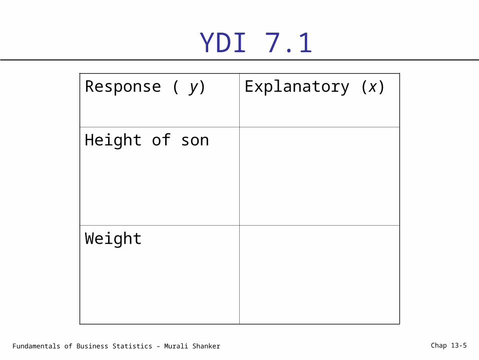
YDI 7.1Response ( y) Explanatory (x)

Height of son

Weight


Scatter Plots and Correlation

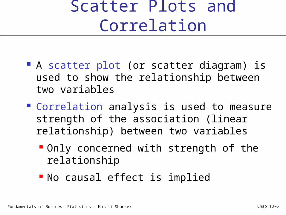
A scatter plot (or scatter diagram) is used to show the relationship between two variables

Correlation analysis is used to measure strength of the association (linear relationship) between two variables

Only concerned with strength of the relationship

No causal effect is implied


Example

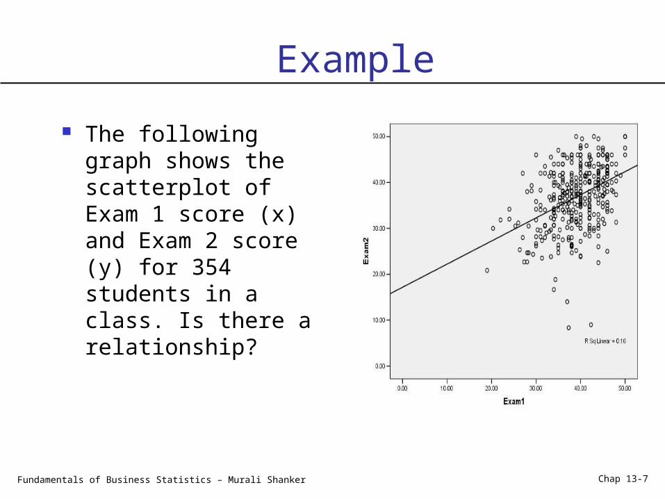
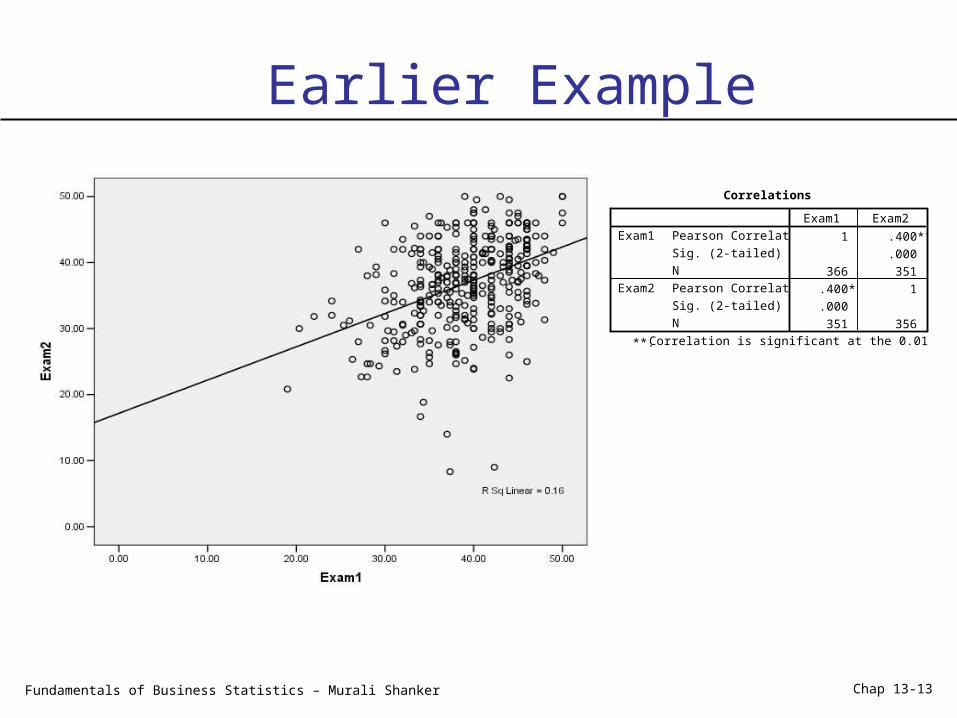
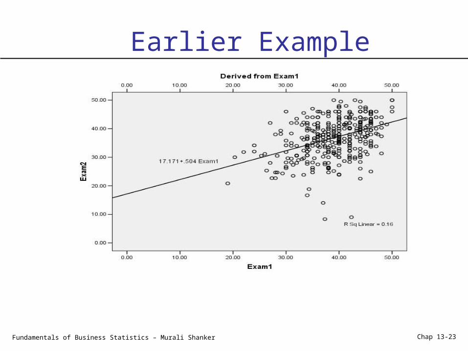
The following graph shows the scatterplot of Exam 1 score (x) and Exam 2 score (y) for 354 students in a class. Is there a relationship?


Scatter Plot Examples

y

x

y

x

y

y

x

x

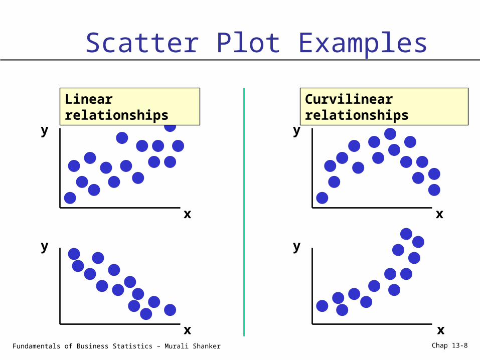
Linear relationships Curvilinear relationships


Scatter Plot Examples

y

x

y

x

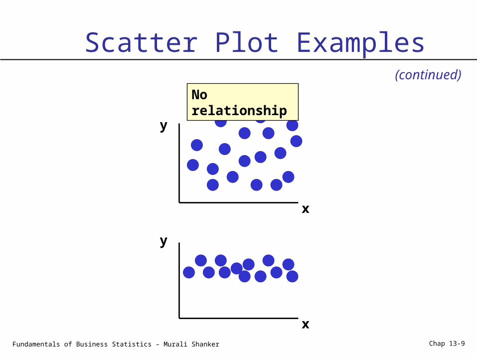
No relationship

(continued)


Correlation Coefficient

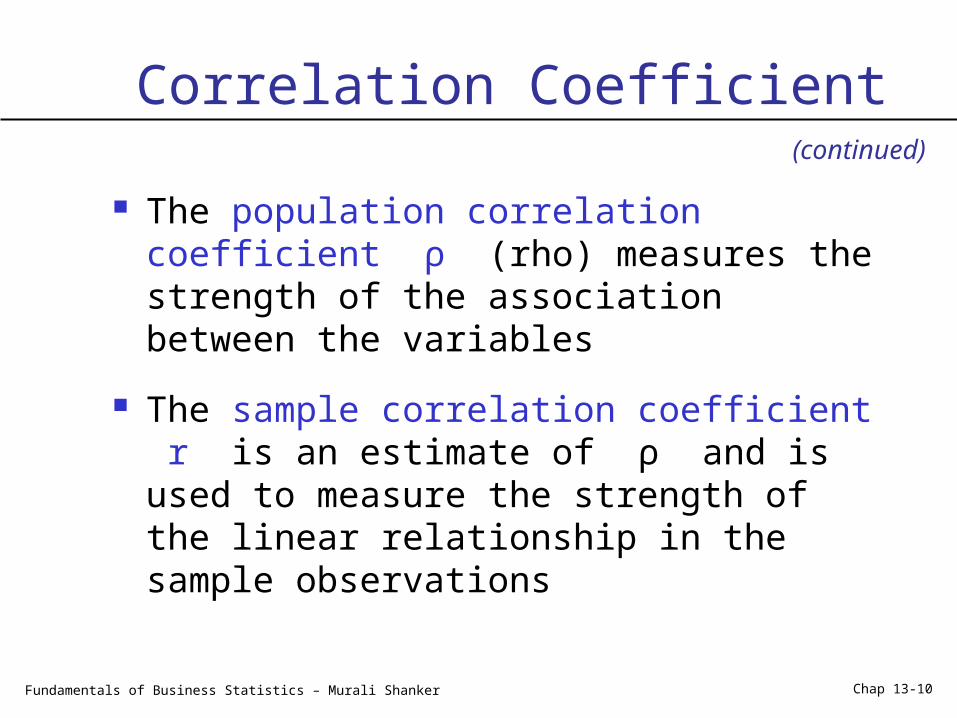
The population correlation coefficient ρ (rho) measures the strength of the association between the variables

The sample correlation coefficient r is an estimate of ρ and is used to measure the strength of the linear relationship in the sample observations

(continued)


Features of ρand r

Unit free Range between -1 and 1 The closer to -1, the stronger the negative

linear relationship The closer to 1, the stronger the positive

linear relationship The closer to 0, the weaker the linear

relationship


Examples of Approximate r Values

y

x

y

x

y

x

y

x

y

x

Tag with appropriate value:

-1, -.6, 0, +.3, 1


Earlier Example

Correlations

1 .400**

.000

366 351

.400** 1

.000

351 356

Pearson Correlation

Sig. (2-tailed)

N

Pearson Correlation

Sig. (2-tailed)

N

Exam1

Exam2

Exam1 Exam2

Correlation is significant at the 0.01 level(2-tailed).

**.


YDI 7.3

What kind of relationship would you expect in the following situations:

age (in years) of a car, and its price.

number of calories consumed per day and weight.

height and IQ of a person.


YDI 7.4

Identify the two variables that vary and decide which should be the independent variable and which should be the dependent variable. Sketch a graph that you think best represents the relationship between the two variables.

1. The size of a persons vocabulary over his or her lifetime.

2. The distance from the ceiling to the tip of the minute hand of a clock hung on the wall.


Introduction to Regression Analysis

Regression analysis is used to: Predict the value of a dependent variable based on

the value of at least one independent variable Explain the impact of changes in an independent

variable on the dependent variable

Dependent variable: the variable we wish to explain

Independent variable: the variable used to explain the dependent variable


Simple Linear Regression Model

Only one independent variable, x

Relationship between x and y is described by a linear function

Changes in y are assumed to be caused by changes in x


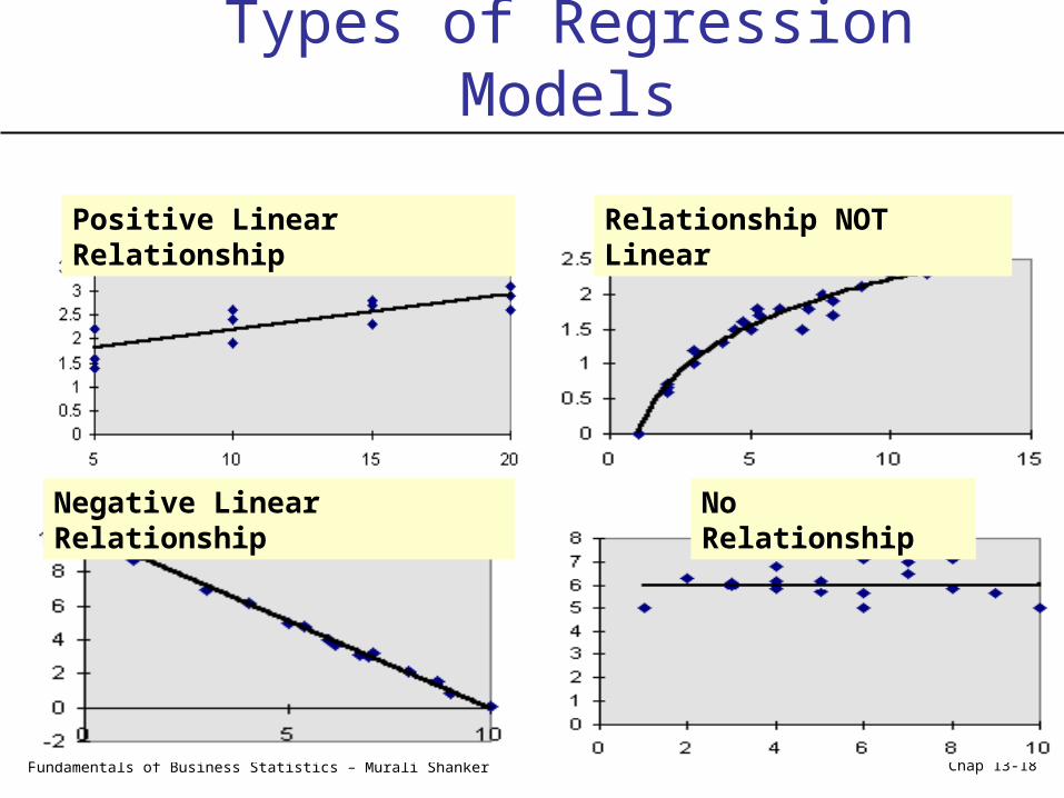
Types of Regression Models

Positive Linear Relationship

Negative Linear Relationship

Relationship NOT Linear

No Relationship


εxββy 10 Linear component

Population Linear Regression

The population regression model:

Population y intercept

Population SlopeCoefficient

Random Error term, or residualDependent

Variable

Independent Variable

Random Error component


Linear Regression Assumptions

Error values (ε) are statistically independent Error values are normally distributed for any

given value of x The probability distribution of the errors is

normal The probability distribution of the errors has

constant variance The underlying relationship between the x

variable and the y variable is linear


Population Linear Regression(continued)

Random Error for this x value

y

x

Observed Value of y for xi

Predicted Value of y for xi

εxββy 10

xi

Slope = β1

Intercept = β0

εi


xbby 10i

The sample regression line provides an estimate of the population regression line

Estimated Regression Model

Estimate of the regression

intercept

Estimate of the regression slope

Estimated (or predicted) y value

Independent variable

The individual random error terms ei have a mean of zero


Earlier Example


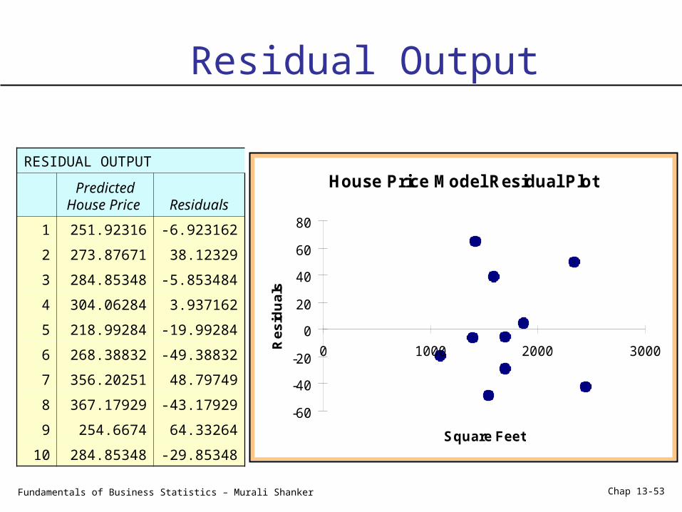
Residual

A residual is the difference between the observed response y and the predicted response ŷ. Thus, for each pair of observations (xi, yi), the ith residual isei = yi − ŷi = yi − (b0 + b1x)


Least Squares Criterion

b0 and b1 are obtained by finding the values of b0 and b1 that minimize the sum of the squared residuals

210

22

x))b(b(y

)y(ye


b0 is the estimated average value of y

when the value of x is zero

b1 is the estimated change in the

average value of y as a result of a one-unit change in x

Interpretation of the Slope and the Intercept


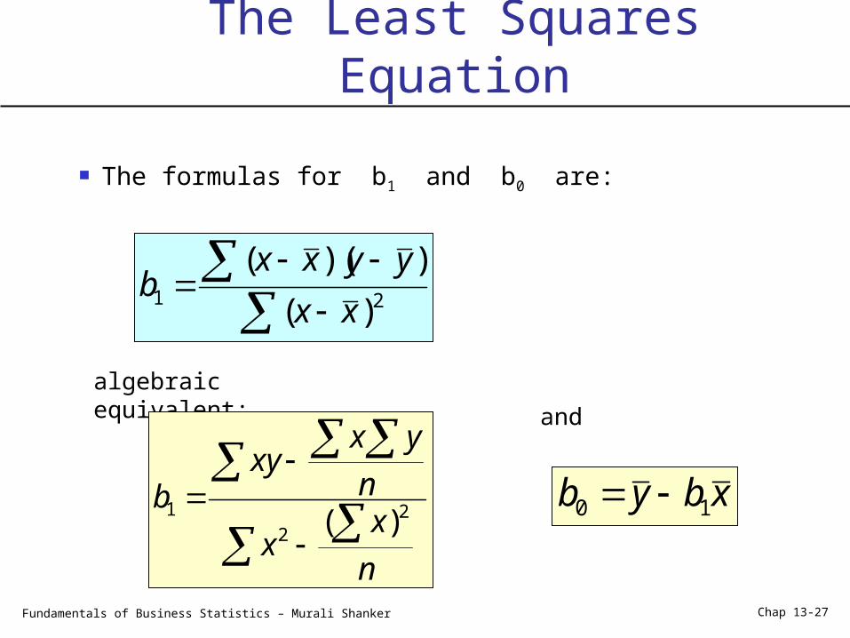
The Least Squares Equation

The formulas for b1 and b0 are:

algebraic equivalent:

n

xx

n

yxxy

b 22

1 )(

21 )(

))((

xx

yyxxb

xbyb 10

and


Finding the Least Squares Equation

The coefficients b0 and b1 will usually be found using computer software, such as Excel, Minitab, or SPSS.

Other regression measures will also be computed as part of computer-based regression analysis


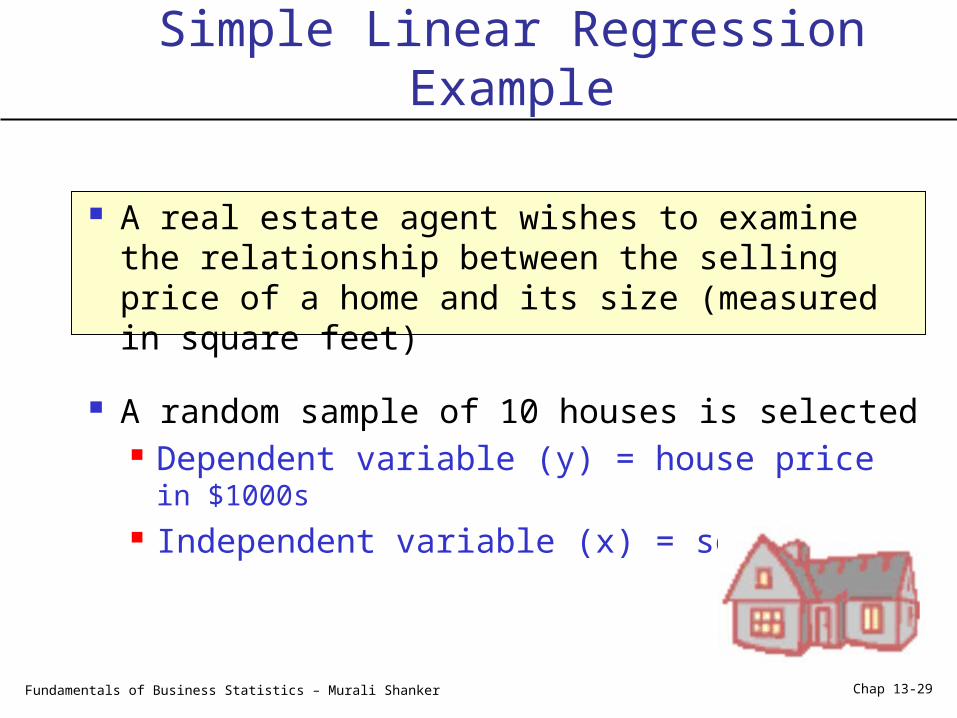
Simple Linear Regression Example

A real estate agent wishes to examine the relationship between the selling price of a home and its size (measured in square feet)

A random sample of 10 houses is selected Dependent variable (y) = house price in $1000s Independent variable (x) = square feet


Sample Data for House Price Model

House Price in $1000s(y)

Square Feet (x)

245 1400

312 1600

279 1700

308 1875

199 1100

219 1550

405 2350

324 2450

319 1425

255 1700


Model Summary

.762a .581 .528 41.33032Model1

R R SquareAdjustedR Square

Std. Error ofthe Estimate

Predictors: (Constant), Square Feeta.

Coefficientsa

98.248 58.033 1.693 .129

.110 .033 .762 3.329 .010

(Constant)

Square Feet

Model1

B Std. Error

UnstandardizedCoefficients

Beta

StandardizedCoefficients

t Sig.

Dependent Variable: House Pricea.

SPSS Output

The regression equation is:

feet) (square 0.110 98.248 price house


0

50

100

150

200

250

300

350

400

450

0 500 1000 1500 2000 2500 3000

Square Feet

Ho

use

Pri

ce (

$100

0s)

Graphical Presentation

House price model: scatter plot and regression line


Slope = 0.110

Intercept = 98.248


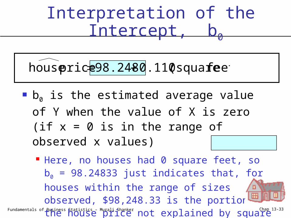
Interpretation of the Intercept, b0

b0 is the estimated average value of Y when the

value of X is zero (if x = 0 is in the range of observed x values)

Here, no houses had 0 square feet, so b0 = 98.24833

just indicates that, for houses within the range of sizes observed, $98,248.33 is the portion of the house price not explained by square feet



Interpretation of the Slope Coefficient, b1

b1 measures the estimated change in the

average value of Y as a result of a one-unit change in X Here, b1 = .10977 tells us that the average value of a

house increases by .10977($1000) = $109.77, on average, for each additional one square foot of size



Least Squares Regression Properties

The sum of the residuals from the least squares regression line is 0 ( )

The sum of the squared residuals is a minimum (minimized )

The simple regression line always passes through the mean of the y variable and the mean of the x variable

The least squares coefficients are unbiased estimates of β0 and β1

0)ˆ( yy

2)ˆ( yy


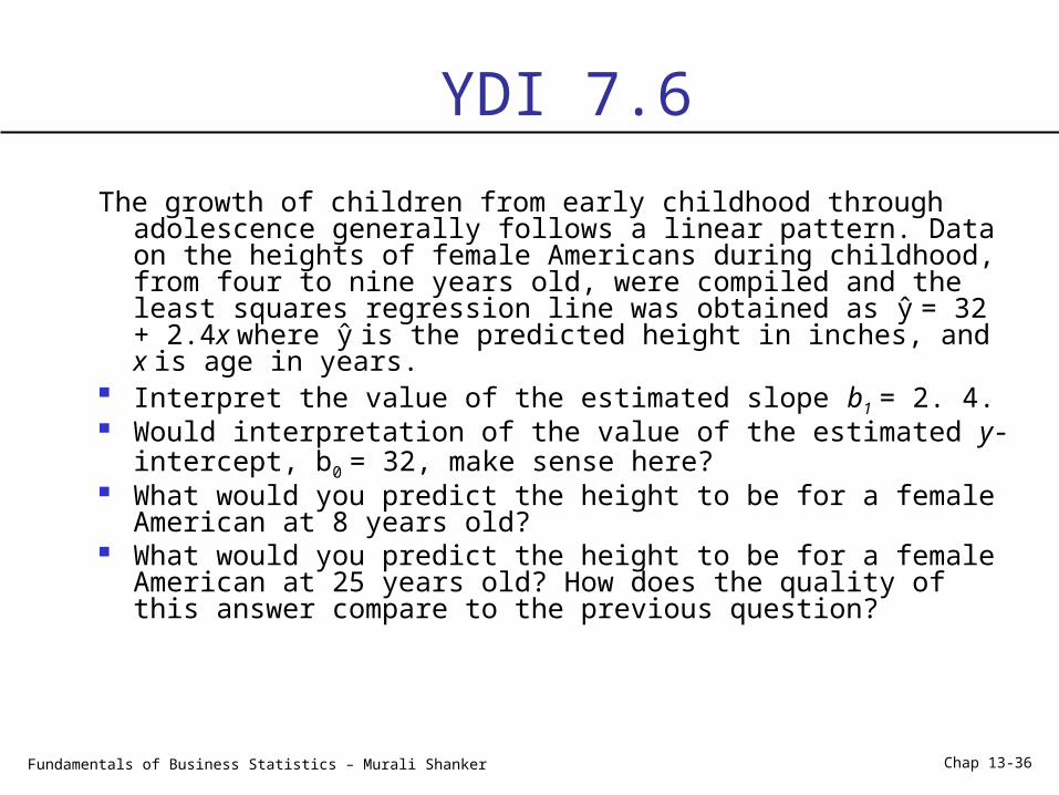
YDI 7.6

The growth of children from early childhood through adolescence generally follows a linear pattern. Data on the heights of female Americans during childhood, from four to nine years old, were compiled and the least squares regression line was obtained as ŷ = 32 + 2.4x where ŷ is the predicted height in inches, and x is age in years.

Interpret the value of the estimated slope b1 = 2. 4. Would interpretation of the value of the estimated y-intercept, b0 =

32, make sense here? What would you predict the height to be for a female American at 8

years old? What would you predict the height to be for a female American at

25 years old? How does the quality of this answer compare to the previous question?


The coefficient of determination is the portion of the total variation in the dependent variable that is explained by variation in the independent variable

The coefficient of determination is also called R-squared and is denoted as R2

Coefficient of Determination, R2

1R0 2


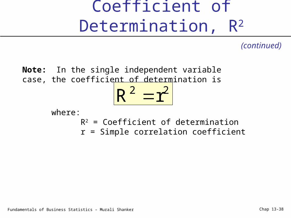
Coefficient of Determination, R2

(continued)

Note: In the single independent variable case, the coefficient of determination is

where:R2 = Coefficient of determination

r = Simple correlation coefficient

22 rR


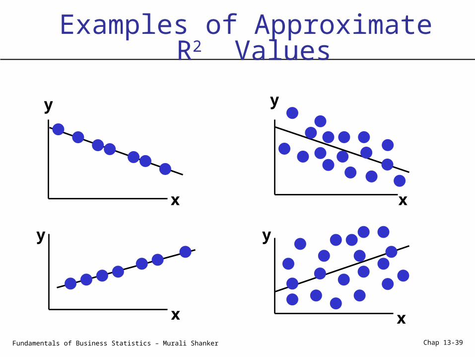
Examples of Approximate R2 Values

y

x

y

x

y

x

y

x


Examples of Approximate R2 Values

R2 = 0

No linear relationship between x and y:

The value of Y does not depend on x. (None of the variation in y is explained by variation in x)

y

xR2 = 0


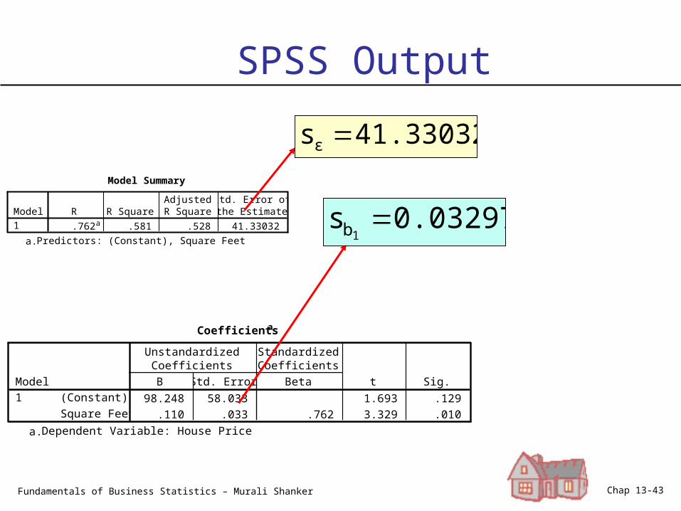
SPSS OutputModel Summary

.762a .581 .528 41.33032Model1




ANOVAb

18934.935 1 18934.935 11.085 .010a

13665.565 8 1708.196

32600.500 9

Regression

Residual

Total

Model1

Sum ofSquares df Mean Square F Sig.


Dependent Variable: House Priceb.

Coefficientsa

98.248 58.033 1.693 .129

.110 .033 .762 3.329 .010

(Constant)

Square Feet

Model1

B Std. Error


Beta


t Sig.



Standard Error of Estimate

The standard deviation of the variation of observations around the regression line is called the standard error of estimate

The standard error of the regression slope coefficient (b1) is given by sb1

s


Model Summary

.762a .581 .528 41.33032Model1




Coefficientsa

98.248 58.033 1.693 .129

.110 .033 .762 3.329 .010

(Constant)

Square Feet

Model1

B Std. Error


Beta


t Sig.


SPSS Output

41.33032sε

0.03297s1b


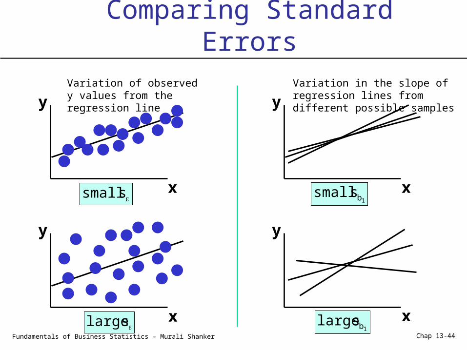
Comparing Standard Errors

y

y y

x

x

x

y

x

1bs small

1bs large

s small

s large

Variation of observed y values from the regression line

Variation in the slope of regression lines from different possible samples


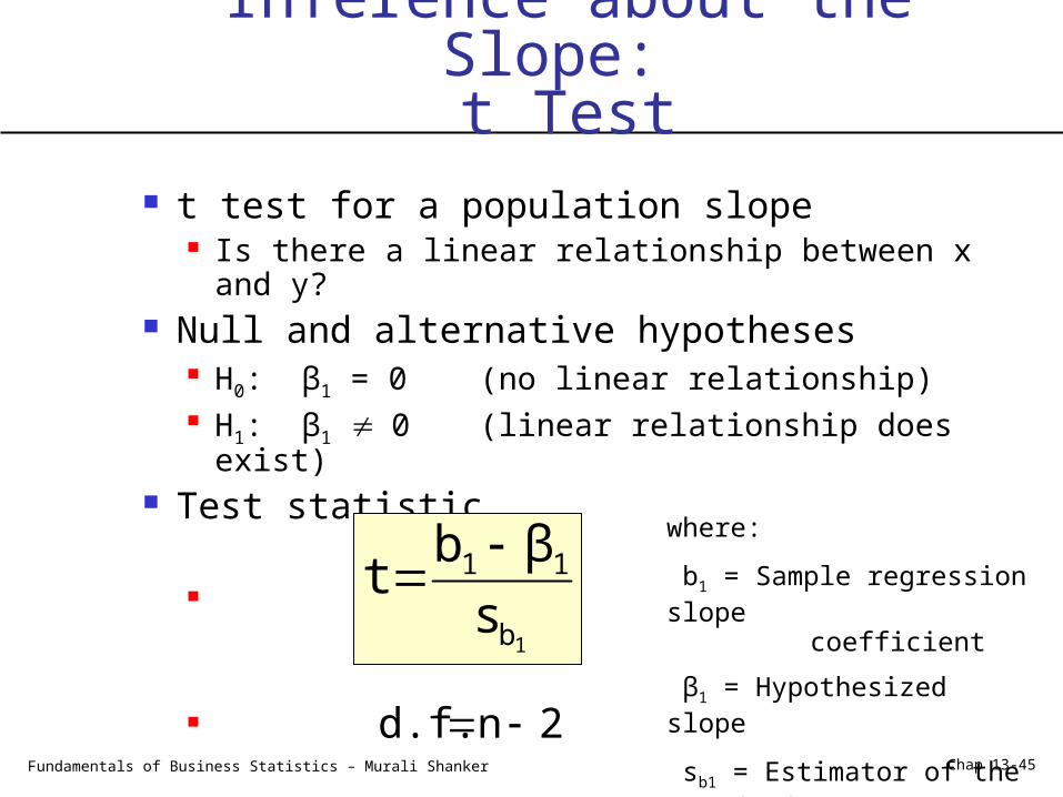
Inference about the Slope: t Test

t test for a population slope Is there a linear relationship between x and y?

Null and alternative hypotheses H0: β1 = 0 (no linear relationship) H1: β1 0 (linear relationship does exist)

Test statistic

1b

11

s

βbt

2nd.f.

where:

b1 = Sample regression slope coefficient

β1 = Hypothesized slope

sb1 = Estimator of the standard error of the slope


House Price in $1000s

(y)

Square Feet (x)

245 1400

312 1600

279 1700

308 1875

199 1100

219 1550

405 2350

324 2450

319 1425

255 1700

(sq.ft.) 0.1098 98.25 price house

Estimated Regression Equation:

The slope of this model is 0.1098

Does square footage of the house affect its sales price?

Inference about the Slope: t Test

(continued)


Inferences about the Slope: t Test Example

H0: β1 = 0

HA: β1 0

Test Statistic: t = 3.329

There is sufficient evidence that square footage affects house price

From Excel output:

Reject H0

Coefficients Standard Error t Stat P-value

Intercept 98.24833 58.03348 1.69296 0.12892

Square Feet 0.10977 0.03297 3.32938 0.01039

1bs tb1

Decision:

Conclusion:

Reject H0Reject H0

/2=.025

-tα/2

Do not reject H0

0 tα/2

/2=.025

-2.3060 2.3060 3.329

d.f. = 10-2 = 8


Regression Analysis for Description

Confidence Interval Estimate of the Slope:

Excel Printout for House Prices:

At 95% level of confidence, the confidence interval for the slope is (0.0337, 0.1858)

1b/211 sb t

Coefficients Standard Error t Stat P-value Lower 95% Upper 95%

Intercept 98.24833 58.03348 1.69296 0.12892 -35.57720 232.07386

Square Feet 0.10977 0.03297 3.32938 0.01039 0.03374 0.18580

d.f. = n - 2


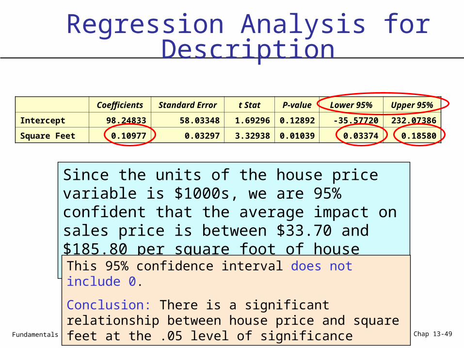
Regression Analysis for Description

Since the units of the house price variable is $1000s, we are 95% confident that the average impact on sales price is between $33.70 and $185.80 per square foot of house size

Coefficients Standard Error t Stat P-value Lower 95% Upper 95%

Intercept 98.24833 58.03348 1.69296 0.12892 -35.57720 232.07386

Square Feet 0.10977 0.03297 3.32938 0.01039 0.03374 0.18580

This 95% confidence interval does not include 0.

Conclusion: There is a significant relationship between house price and square feet at the .05 level of significance


Residual Analysis

Purposes Examine for linearity assumption Examine for constant variance for all

levels of x Evaluate normal distribution assumption

Graphical Analysis of Residuals Can plot residuals vs. x Can create histogram of residuals to

check for normality


Residual Analysis for Linearity

Not Linear Linear

x

resi

dua

ls

x

y

x

y

x

resi

dua

ls


Residual Analysis for Constant Variance

Non-constant variance Constant variance

x x

y

x x

y

resi

dua

ls

resi

dua

ls


House Price Model Residual Plot

-60

-40

-20

0

20

40

60

80

0 1000 2000 3000

Square Feet

Re

sid

ua

ls

Residual Output

RESIDUAL OUTPUT

Predicted House Price Residuals

1 251.92316 -6.923162

2 273.87671 38.12329

3 284.85348 -5.853484

4 304.06284 3.937162

5 218.99284 -19.99284

6 268.38832 -49.38832

7 356.20251 48.79749

8 367.17929 -43.17929

9 254.6674 64.33264

10 284.85348 -29.85348

Date post:	21-Dec-2015
Category:	Documents
View:	217 times
Download:	0 times

Fundamentals of Business Statistics – Murali Shanker Chap 13-1 Business Statistics: A...

Documents