279
| Date post: | 02-Jan-2016 |
| Category: |
Documents |
| Upload: | jorge-rodriguez |
| View: | 62 times |
| Download: | 4 times |
FUNDAMENTALS OFNUMERICAL COMPUTING
L. F. ShampineSouthern Methodist University
R. C. Allen, Jr.Sandia National Laboratories
S. PruessColorado School of Mines
JOHN WILEY & SONS, INC.New York Chichester Brisbane Toronto Singapore

Acquisitions Editor Barbara HollandEditorial Assistant Cindy RhoadsMarketing Manager Cathy FaduskaSenior Production Manager Lucille BuonocoreSenior Production Editor Nancy PrinzManufacturing Manager Murk CirilloCover Designer Steve Jenkins
This book was set in Times Roman, and was printed and bound by R.R. Donnelley &Sons Company, Crawfordsville. The cover was printed by The Lehigh Press, Inc.
Recognizing the importance of preserving what has been written, it is apolicy of John Wiley & Sons, Inc. to have books of enduring value publishedin the United States printed on acid-free paper, and we exert our bestefforts to that end.
The paper in this book was manufactured by a mill whose forest management programsinclude sustained yield harvesting of its timberlands. Sustained yield harvestingprinciples ensure that the number of trees cut each year does not exceed the amount ofnew growth.
Copyright © 1997, by John Wiley & Sons, Inc.
All rights reserved. Published simultaneously in Canada.
Reproduction or translation of any part ofthis work beyond that permitted by Sections107 and 108 of the 1976 United States CopyrightAct without the permission of the copyrightowner is unlawful. Requests for permissionor further information should be addressed tothe Permissions Department, John Wiley & Sons, Inc.
Library of Congress Cataloging-in-Publication Data:Shampine, LawrenceFundamentals of numerical computing / Richard Allen, StevePruess, Lawrence Shampine.p. cm.Includes bibliographical reference and index.ISBN 0-471-16363-5 (cloth : alk. paper)1. Numerical analysis-Data processing. I. Pruess, Steven.II. Shampine, Lawrence F. III. Title.QA297.A52 1997519.4’0285’51—dc20 96-22074
CIPPrinted in the United States of America
10 9 8 7 6 5 4 3 2 1
PRELIMINARIES
The purpose of this book is to develop the understanding of basic numerical meth-ods and their implementations as software that are necessary for solving fundamentalmathematical problems by numerical means. It is designed for the person who wantsto do numerical computing. Through the examples and exercises, the reader studies thebehavior of solutions of the mathematical problem along with an algorithm for solv-ing the problem. Experience and understanding of the algorithm are gained throughhand computation and practice solving problems with a computer implementation. Itis essential that the reader understand how the codes provided work, precisely whatthey do, and what their limitations are. The codes provided are powerful, yet simpleenough for pedagogical use. The reader is exposed to the art of numerical computingas well as the science.
The book is intended for a one-semester course, requiring only calculus and amodest acquaintance with FORTRAN, C, C++, or MATLAB. These constraints ofbackground and time have important implications: the book focuses on the problemsthat are most common in practice and accessible with the background assumed. Byconcentrating on one effective algorithm for each basic task, it is possible to developthe fundamental theory in a brief, elementary way. There are ample exercises, andcodes are provided to reduce the time otherwise required for programming and debug-ging. The intended audience includes engineers, scientists, and anyone else interestedin scientific programming. The level is upper-division undergraduate to beginninggraduate and there is adequate material for a one semester to two quarter course.
Numerical analysis blends mathematics, programming, and a considerable amountof art. We provide programs with the book that illustrate this. They are more than mereimplementations in a particular language of the algorithms presented, but they are notproduction-grade software. To appreciate the subject fully, it will be necessary to studythe codes provided and gain experience solving problems first with these programs andthen with production-grade software.
Many exercises are provided in varying degrees of difficulty. Some are designedto get the reader to think about the text material and to test understanding, while othersare purely computational in nature. Problem sets may involve hand calculation, alge-braic derivations, straightforward computer solution, or more sophisticated computingexercises.
The algorithms that we study and implement in the book are designed to avoidsevere roundoff errors (arising from the finite number of digits available on computersand calculators), estimate truncation errors (arising from mathematical approxima-tions), and give some indication of the sensitivity of the problem to errors in the data.In Chapter 1 we give some basic definitions of errors arising in computations andstudy roundoff errors through some simple but illuminating computations. Chapter 2deals with one of the most frequently occurring problems in scientific computation,the solution of linear systems of equations. In Chapter 3 we deal with the problem of
V
vi PRELIMINARIES
interpolation, one of the most fundamental and widely used tools in numerical com-putation. In Chapter 4 we study methods for finding solutions to nonlinear equations.Numerical integration is taken up in Chapter 5 and the numerical solution of ordinarydifferential equations is examined in Chapter 6. Each chapter contains a case studythat illustrates how to combine analysis with computation for the topic of that chapter.
Before taking up the various mathematical problems and procedures for solvingthem numerically, we need to discuss briefly programming languages and acquisitionof software.
PROGRAMMING LANGUAGES
The FORTRAN language was developed specifically for numerical computation andhas evolved continuously to adapt it better to the task. Accordingly, of the widelyused programming languages, it is the most natural for the programs of this book. TheC language was developed later for rather different purposes, but it can be used fornumerical computation.
At present FORTRAN 77 is very widely available and codes conforming to theANSI standard for the language are highly portable, meaning that they can be movedto another hardware/software configuration with very little change. We have chosento provide codes in FORTRAN 77 mainly because the newer Fortran 90 is not in wideuse at this time. A Fortran 90 compiler will process correctly our FORTRAN 77programs (with at most trivial changes), but if we were to write the programs so asto exploit fully the new capabilities of the language, a number of the programs wouldbe structured in a fundamentally different way. The situation with C is similar, butin our experience programs written in C have not proven to be nearly as portable asprograms written in standard FORTRAN 77. As with FORTRAN, the C language hasevolved into C++, and as with Fortran 90 compared to FORTRAN 77, exploiting fullythe additional capabilities of C++ (in particular, object oriented programming) wouldlead to programs that are completely different from those in C. We have opted for amiddle ground in our C++ implementations.
In the last decade several computing environments have been developed. Popularones familiar to us are MATLAB [l] and Mathematica [2]. MATLAB is very much inkeeping with this book, for it is devoted to the solution of mathematical problems bynumerical means. It integrates the formation of a mathematical model, its numericalsolution, and graphical display of results into a very convenient package. Many of thetasks we study are implemented as a single command in the MATLAB language. AsMATLAB has evolved, it has added symbolic capabilities. Mathematica is a similarenvironment, but it approaches mathematical problems from the other direction. Orig-inally it was primarily devoted to solving mathematical problems by symbolic means,but as it has evolved, it has added significant numerical capabilities. In the book werefer to the numerical methods implemented in these widely used packages, as wellas others, but we mention the packages here because they are programming languagesin their own right. It is quite possible to implement the algorithms of the text in theselanguages. Indeed, this is attractive because the environments deal gracefully with anumber of issues that are annoying in general computing using languages like FOR-TRAN or C.
SOFTWARE vii
At present we provide programs written in FORTRAN 77, C, C++, and MATLAB
that have a high degree of portability. Quite possibly in the future the programs willbe made available in other environments (e.g., Fortran 90 or Mathematica.)
SOFTWARE
In this section we describe how to obtain the source code for the programs that ac-company the book and how to obtain production-grade software. It is assumed that thereader has available a browser for the World Wide Web, although some of the softwareis available by ftp or gopher.
The programs that accompany this book are currently available by means of anony-mous ftp (log in as anonymous or as ftp) at
ftp.wiley.com
in subdirectories of public/college/math/sapcodes for the various languages discussedin the preceding section.
The best single source of software is the Guide to Available Mathematical Soft-ware (GAMS) developed by the National Institute of Standards and Technology (NIST).It is an on-line cross-index of mathematical software and a virtual software repository.Much of the high-quality software is free. For example, GAMS provides a link tonetlib, a large collection of public-domain mathematical software. Most of the pro-grams in netlib are written in FORTRAN, although some are in C. A number of thepackages found in netlib are state-of-the-art software that are cited in this book. Theinternet address is
http://gams.nist.gov
for GAMS.A useful source of microcomputer software and pointers to other sources of soft-
ware is the Mathematics Archives at
http://archives.math.utk.edu:80/
It is worth remarking that one item listed there is an “Index of resources for numericalcomputation in C or C++.”
There are a number of commercial packages that can be located by means ofGAMS. We are experienced with the NAG and IMSL libraries, which are large col-lections of high-quality mathematical software found in most computing centers. Thecomputing environments MATLAB and Mathematica mentioned in the preceding sec-tion can also be located through GAMS.
REFERENCES
1. C. Moler, J. Little, S. Bangert, and S. Kleiman,Mass., 1987. email: [email protected]
ProMatlab User’s Guide, MathWorks, Sherborn,
2. S. Wolfram, Mathematica, Addison-Wesley, Redwood City, Calif., 1991. email: [email protected]
viii PRELIMINARIES
ACKNOWLEDGMENTS
The authors are indebted to many individuals who have contributed to the productionof this book. Professors Bernard Bialecki and Michael Hosea have been especiallysharp-eyed at catching errors in the latest versions. We thank the people at Wiley, Bar-bara Holland, Cindy Rhoads, and Nancy Prinz, for their contributions. David Richardsat the University of Illinois played a critical role in getting the functioningfor us, and quickly and accurately fixing other We also acknowledgethe work of James Otto in checking all solutions and examples, and Hong-sung Jinwho generated most of the figures. Last, but certainly not least, we are indeed gratefulto the many students, too numerous to mention, who have made valuable suggestionsto us over the years.
CONTENTS
CHAPTER 1 ERRORS AND FLOATING POINT ARITHMETIC 11.1 Basic Concepts 1
1.2 Examples of Floating Point Calculations 12
1.3 Case Study 1 25
1.4 Further Reading 28
CHAPTER 2 SYSTEMS OF LINEAR EQUATIONS 302.1 Gaussian Elimination with Partial Pivoting 32
2.2 Matrix Factorization 44
2.3 Accuracy 48
2.4 Routines Factor and Solve 61
2.5 Matrices with Special Structure 65
2.6 Case Study 2 72
CHAPTER 3 INTERPOLATION 823.1 Polynomial Interpolation 83
3.2 More Error Bounds 90
3.3 Newton Divided Difference Form 93
3.4 Assessing Accuracy 98
3.5 Spline Interpolation 101
3.6 Interpolation in the Plane 119
3.7 Case Study 3 128
CHAPTER 4 ROOTS OF NONLINEAR EQUATIONS 1344.1 Bisection, Newton’s Method, and the Secant Rule 137
4.2 An Algorithm Combining Bisection and the Secant Rule 150
4.3 Routines for Zero Finding 152
4.4 Condition, Limiting Precision, and Multiple Roots 157
4.5 Nonlinear Systems of Equations 1604.6 Case Study 4 163
ix
X CONTENTS
CHAPTER 5 NUMERICAL INTEGRATION 1705.1 Basic Quadrature Rules 170
5.2 Adaptive Quadrature 184
5.3 Codes for Adaptive Quadrature 188
5.4 Special Devices for Integration 191
5.5 Integration of Tabular Data 200
5.6 Integration in Two Variables 202
5.7 Case Study 5 203
CHAPTER 6 ORDINARY DIFFERENTIAL EQUATIONS 2106.1 Some Elements of the Theory 210
6.2 A Simple Numerical Scheme 216
6.3 One-Step Methods 221
6.4 Errors-Local and Global 228
6.5 The Algorithms 233
6.6 The Code Rke 236
6.7 Other Numerical Methods 240
6.8 Case Study 6 244
APPENDIX A NOTATION AND SOME THEOREMS FROM THECALCULUS 251A.1 Notation 251
A.2 Theorems 252
ANSWERS TO SELECTED EXERCISES 255
INDEX 266
CHAPTER 1
ERRORS AND FLOATING POINTARITHMETIC
Errors in mathematical computation have several sources. One is the modeling thatled to the mathematical problem, for example, assuming no wind resistance in study-ing projectile motion or ignoring finite limits of resources in population and economicgrowth models. Such errors are not the concern of this book, although it must be keptin mind that the numerical solution of a mathematical problem can be no more mean-ingful than the underlying model. Another source of error is the measurement of datafor the problem. A third source is a kind of mathematical error called discretizationor truncation error. It arises from mathematical approximations such as estimating anintegral by a sum or a tangent line by a secant line. Still another source of error is theerror that arises from the finite number of digits available in the computers and cal-culators used for the computations. It is called roundoff error. In this book we studythe design and implementation of algorithms that aim to avoid severe roundoff errors,estimate truncation errors, and give some indication of the sensitivity of the problemto errors in the data. This chapter is devoted to some fundamental definitions and astudy of roundoff by means of simple but illuminating computations.
1.1 BASIC CONCEPTS
How well a quantity is approximated is measured in two ways:
absolute error = true value - approximate value
relative error =true value - approximate value
true value.
Relative error is not defined if the true value is zero. In the arithmetic of computers,relative error is the more natural concept, but absolute error may be preferable whenstudying quantities that are close to zero.
A mathematical problem with input (data) x and output (answer) y = F(x) is saidto be well-conditioned if “small” changes in x lead to “small” changes in y. If the
1
2 CHAPTER 1 ERRORS AND FLOATING POINT ARITHMETIC
changes in y are “large,” the problem is said to be ill-conditioned. Whether a problemis well- or ill-conditioned can depend on how the changes are measured. A conceptrelated to conditioning is stability. It is concerned with the sensitivity of an algorithmfor solving a problem with respect to small changes in the data, as opposed to the sen-sitivity of the problem itself. Roundoff errors are almost inevitable, so the reliabilityof answers computed by an algorithm depends on whether small roundoff errors mightseriously affect the results. An algorithm is stable if “small” changes in the input leadto “small” changes in the output. If the changes in the output are “large,” the algorithmis unstable.
To gain some insight about condition, let us consider a differentiable function F(x)and suppose that its argument, the input, is changed from x to x + εx. This is a relativechange of ε in the input data. According to Theorem 4 of the appendix, the changeinduces an absolute change in the output value F(x) of
F(x) - F( x+εx ) (x).
The relative change is
F (x) - F(x+ εx ) F´(x)
F(x) F(x) .
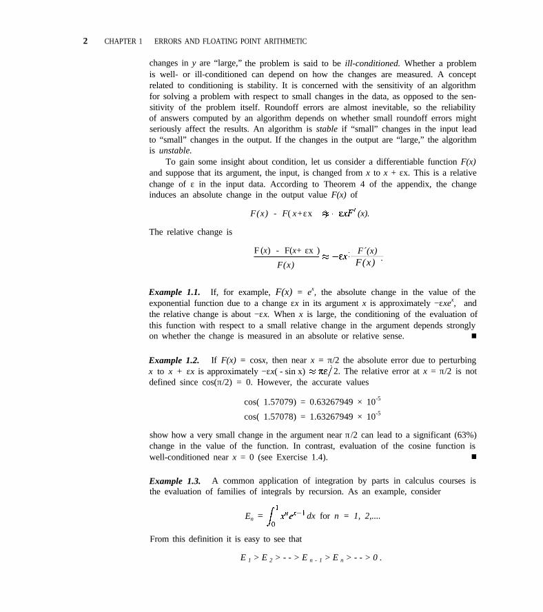
Example 1.1. If, for example, F(x) = ex, the absolute change in the value of theexponential function due to a change εx in its argument x is approximately −εxex, andthe relative change is about −εx. When x is large, the conditioning of the evaluation ofthis function with respect to a small relative change in the argument depends stronglyon whether the change is measured in an absolute or relative sense. n
Example 1.2. If F(x) = cosx, then near x = π/2 the absolute error due to perturbingx to x + εx is approximately −εx( - sin x) 2. The relative error at x = π/2 is notdefined since cos(π/2) = 0. However, the accurate values
cos( 1.57079) = 0.63267949 × 10⁻⁵
cos( 1.57078) = 1.63267949 × 10⁻⁵
show how a very small change in the argument near π/2 can lead to a significant (63%)change in the value of the function. In contrast, evaluation of the cosine function iswell-conditioned near x = 0 (see Exercise 1.4). n
Example 1.3. A common application of integration by parts in calculus courses isthe evaluation of families of integrals by recursion. As an example, consider
En = dx for n = 1, 2,....
From this definition it is easy to see that
E 1 > E 2 > - - > E n - 1 > E n > - - > 0 .
1.1 BASIC CONCEPTS 3
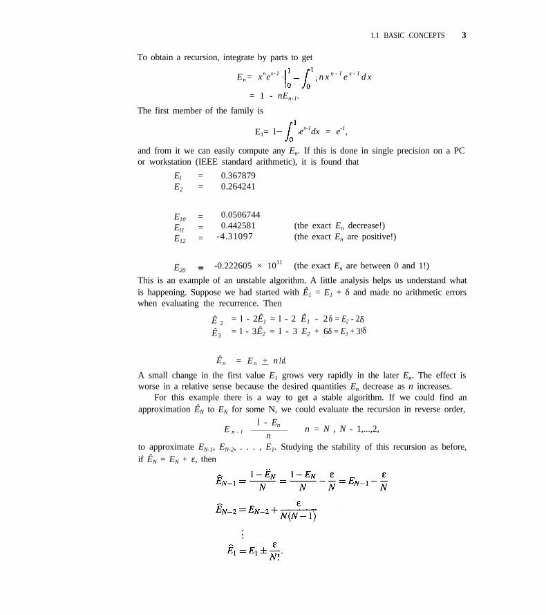
To obtain a recursion, integrate by parts to get
En= xnex-1 n x n - 1 e x - 1 d x
= 1 - nEn-1.
The first member of the family is
E1= l ex-1dx = e-1,
and from it we can easily compute any En. If this is done in single precision on a PCor workstation (IEEE standard arithmetic), it is found that
El = 0.367879E2 = 0.264241
E10 = 0.0506744
El1 = 0.442581 (the exact En decrease!)
E12 = -4.31097 (the exact En are positive!)
E20 = -0.222605 × 10¹¹ (the exact En are between 0 and 1!)
This is an example of an unstable algorithm. A little analysis helps us understand whatis happening. Suppose we had started with Ê1 = E1 + δ and made no arithmetic errorswhen evaluating the recurrence. Then
Ê 2= l - 2Ê1 = l - 2 Ê1 - 2δ = E2 - 2δ
Ê3= l - 3Ê2 = l - 3 E2 + 6δ = E3 + 3!δ
Ên = En + n!δ.
A small change in the first value E1 grows very rapidly in the later En. The effect isworse in a relative sense because the desired quantities En decrease as n increases.
For this example there is a way to get a stable algorithm. If we could find anapproximation ÊN to EN for some N, we could evaluate the recursion in reverse order,
l - EnE n - l n
n = N , N - 1,...,2,
to approximate EN-1, EN-2, . . . , E1. Studying the stability of this recursion as before,if ÊN = EN + ε, then
4 CHAPTER 1 ERRORS AND FLOATING POINT ARITHMETIC
The recursion is so cheap and the error damps out so quickly that we can start with apoor approximation ÊN for some large N and get accurate answers inexpensively forthe En that really interest us. Notice that recurring in this direction, the En increase,making the relative errors damp out even faster. The inequality
0 < E n < xndx =1
n + 1
shows how to easily get an approximation to En with an error that we can bound. Forexample, if we take N = 20, the crude approximation Ê20 = 0 has an absolute error lessthan l/21 in magnitude. The magnitude of the absolute error in Ê19 is then less thanl/(20 × 21) = 0.0024,. . . , and that in Ê15 is less than 4 × 10⁻⁸. The approximationsto E14,. . . , E1 will be even more accurate.
A stable recurrence like the second algorithm is the standard way to evaluate cer-tain mathematical functions. It can be especially convenient for a series expansion inthe functions. For example, evaluation of an expansion in Bessel functions of the firstkind,
f(x)= a n J n (x ) ,
requires the evaluation of Jn(x) foraccomplished very inexpensively.
many n. Using recurrence on the index n, this isn
Any real number y 0 can be written in scientific notation as
y = ±.d1d2···d s d s + 1 ···×10 e (1.1)
Here there are an infinite number of digits di. Each di takes on one of the values
0, 1,..., 9 and we assume the number y is normalized so that d1 > 0. The portion.dld2... is called the fraction or mantissa or significand; it has the meaning
dl × 10-l + d2 × 10-2 + ··· + ds × 10- s + ··· .
There is an ambiguity in this representation; for example, we must agree that
0.24000000 ···
is the same as
0.23999999 ··· .
The quantity e in (1.1) is called the exponent; it is a signed integer.Nearly all numerical computations on a digital computer are done in floating point
arithmetic. This is a number system that uses a finite number of digits to approximatethe real number system used for exact computation. A system with s digits and base10 has all of its numbers of the form
y = ±.dld2 ··· ds × 10e . (1.2)
1.1 BASIC CONCEPTS 5
Again, for nonzero numbers each di is one of the digits 0, 1,...,9 and d1 > 0 for anormalized number. The exponent e also has only a finite number of digits; we assumethe range
The number zero is special; it is written as
0.0 ··· 0 × 10m ?
Example 1.4. If s = l, m = -1, and M = 1, then the set of floating point numbers is
+0.l × 10-1, +0.2 × 10⁻¹, ...) +0.9 × 10⁻¹
+0.l × 10 0 , +0.2 × 10 0 , . . . ) +0.9 × 10 0
+0.l × 101) +0.2 × 101, ...) +0.9 × 101,
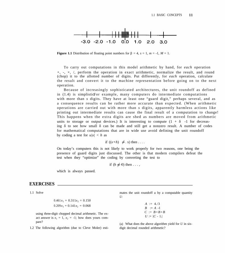
together with the negative of each of these numbers and 0.0 × 10-l for zero. There areonly 55 numbers in this floating point number system. In floating point arithmetic thenumbers are not equally spaced. This is illustrated in Figure 1.1, which is discussedafter we consider number bases other than decimal. n
Because there are only finitely many floating point numbers to represent the realnumber system, each floating point number must represent many real numbers. Whenthe exponent e in (1.1) is bigger than M, it is not possible to represent y at all. If inthe course of some computations a result arises that would need an exponent e > M,the computation is said to have overflowed. Typical operating systems will terminatethe run on overflow. The situation is less clear when e < m, because such a y mightreasonably be approximated by zero. If such a number arises during a computation,the computation is said to have underflowed. In scientific computation it is usually ap-propriate to set the result to zero and continue. Some operating systems will terminatethe run on underflow and others will set the result to zero and continue. Those thatcontinue may report the number of under-flows at the end of the run. If the response ofthe operating system is not to your liking, it is usually possible to change the responseby means of a system routine.
Overflows and underflows are not unusual in scientific computation. For exam-ple, exp(y) will overflow for y > 0 that are only moderately large, and exp(-y) willunderflow. Our concern should be to prevent going out of range unnecessarily.
FORTRAN and C provide for integer arithmetic in addition to floating point arith-metic. Provided that the range of integers allowed is not exceeded, integer arithmeticis exact. It is necessary to beware of overflow because the typical operating systemdoes not report an integer overflow; the computation continues with a number that isnot related to the correct value in an obvious way.
Both FORTRAN and C provide for two precisions, that is, two arithmetics withdifferent numbers of digits s, called single and double precision. The languages dealwith mixing the various modes of arithmetic in a sensible way, but the unwary can getinto trouble. This is more likely in FORTRAN than C because by default, constants inC are double precision numbers. In FORTRAN the type of a constant is taken from the

6 CHAPTER 1 ERRORS AND FLOATING POINT ARITHMETIC
way it is written. Thus, an expression like (3/4)*5. in FORTRAN and in C means thatthe integer 3 is to be divided by the integer 4 and the result converted to a floating pointnumber for multiplication by the floating point number 5. Here the integer division 3/4results in 0, which might not be what was intended. It is surprising how often usersruin the accuracy of a calculation by providing an inaccurate value for a basic constantlike π Some constants of this kind may be predefined to full accuracy in a compileror a library, but it should be possible to use intrinsic functions to compute accuratelyconstants like π = acos(-1.0).
Evaluation of an asymptotic expansion for the special function Ei(x), called theexponential integral, involves computing terms of the form n!/xn. To contrast com-putations in integer and floating point arithmetic, we computed terms of this form fora range of n and x = 25 using both integer and double precision functions for thefactorial. Working in C on a PC using IEEE arithmetic, it was found that the resultsagreed through n = 7, but for larger n the results computed with integer arithmetic wereuseless-the result for n = 8 was negative! The integer overflows that are responsiblefor these erroneous results are truly dangerous because there was no indication fromthe system that the answers might not be reliable.
Example 1.5. In Chapter 4 we study the use of bisection to find a number z suchthat f(z) = 0, that is, we compute a root of f(x). Fundamental to this procedure isthe question, Do f(a) and f(b) have opposite signs? If they do, a continuous functionf(x) has a root z between a and b. Many books on programming provide illustrativeprograms that test for f(a)f(b) < 0. However, when f(a) and f(b) are sufficientlysmall, the product underflows and its sign cannot be determined. This is likely tohappen because we are interested in a and b that tend to z, causing f(a) and f(b) totend to zero. It is easy enough to code the test so as to avoid the difficulty; it is justnecessary to realize that the floating point number system does not behave quite likethe real number system in this test. n
As we shall see in Chapter 4, finding roots of functions is a context in whichunderflow is quite common. This is easy to understand because the aim is to find a zthat makes f(z) as small as possible.
Example 1.6. Determinants. In Chapter 2 we discuss the solution of a system oflinear equations. As a by-product of the algorithm and code presented there, the deter-minant of a system of n equations can be computed as the product of a set of numbersreturned:
de t = y1 y2 ···yn.
Unfortunately, this expression is prone to unnecessary under- and overflows. If, forexample, M = 100 and yl = 1050, y2 = 1060, y3 = 10-30, all the numbers are in rangeand so is the determinant 1080. However, if we form (yl × y2) × y3, the partial productyl × y2 overflows. Note that yl × (y2 × y3) can be formed. This illustrates the fact thatfloating point numbers do not always satisfy the associative law of multiplication thatis true of real numbers.
1.1 BASIC CONCEPTS 7
The more fundamental issue is that because det(cA) = cndet(A), the determinantis extremely sensitive to the scale of the matrix A when the number of equations nis large. A software remedy used in LINPACK [4] in effect extends the range ofexponents available. Another possibility is to use logarithms and exponentials:
l n | d e t | = ln|y i|
|det|=exp(ln|det|).
If this leads to an overflow, it is because the answer cannot be represented in the float-ing point number system. n
Example 1.7. Magnitude. When computing the magnitude of a complex numberz = x + i y ,
there is a difficulty when either x or y is large. Suppose that If |x| is suf-ficiently large, x2 will overflow and we are not able to compute |z| even when it is avalid floating point number. If the computation is reformulated as
the difficulty is avoided. Notice that underflow could occur when |y| << |x|. This isharmless and setting the ratio y/x to zero results in a computed |z| that has a smallrelative error.
The evaluation of the Euclidean norm of a vector v = (v 1 , v 2 , . . . , v n) ,
involves exactly the same kind of computations. Some writers of mathematical soft-ware have preferred to work with the maximum norm
because it avoids the unnecessary overflows and underflows that are possible with astraightforward evaluation of the Euclidean norm. n
If a real number y has an exponent in the allowed range, there are two standardways to approximate it by a floating point number fl(y). If all digits after the first sin (1.1) are dropped, the result is known as a chopped or truncated representation. Afloating point number that is usually closer to y can be found by adding 5 × 10-(s+1)
to the fraction in (1.1) and then chopping. This is called rounding.
Example 1.8. If m = -99, M = 99, s = 5, and π = 3.1415926..., then in choppedarithmetic
fl(π) = 0.31415 × 101
8 CHAPTER 1 ERRORS AND FLOATING POINT ARITHMETIC
while
fl(π) = 0.31416 ×
in rounded arithmetic.
101
n
If the representation (1.1) of y is chopped to s digits, the relative error of fl(y) hasmagnitude
In decimal arithmetic with s digits the unit roundoff u is defined to be 101-s whenchopping is done. In a similar way it is found that
when rounding is done. In this case u is defined to be ½101-s. In either case, u is abound on the relative error of representing a nonzero real number as a floating pointnumber.
Because fl(y) is a real number, for theoretical purposes we can work with it likeany other real number. In particular, it is often convenient to define a real number δsuch that
fl(y) = y(1 + δ).
In general, all we know about δ is the bound
Example 1.9. Impossible accuracy. Modern codes for the computation of a root ofan equation, a definite integral, the solution of a differential equation, and so on, tryto obtain a result with an accuracy specified by the user. Clearly it is not possibleto compute an answer more accurate than the floating point representation of the truesolution. This means that the user cannot be allowed to ask for a relative error smallerthan the unit roundoff u. It might seem odd that this would ever happen, but it does.One reason is that the user does not know the value of u and just asks for too muchaccuracy. A more common reason is that the user specifies an absolute error r. Thismeans that any number y* will be acceptable as an approximation to y if
1.1 BASIC CONCEPTS 9
Such a r eques t co r responds to a sk ing fo r a r e l a t ive e r ro r o f
When |r/y| < u, that is, r < u|y|, this is an impossible request. If the true solution isunexpectedly large, an absolute error tolerance that seems modest may be impossiblein practice. Codes that permit users to specify an absolute error tolerance need tobe able to monitor the size of the solution and warn the user when the task posed isi m p o s s i b l e . n
There is a further complication to the floating point number system-most com-puters do not work with decimal numbers. The common bases are β = 2, binary arith-metic, and β = 16, hexadecimal arithmetic, rather than β = 10, decimal arithmetic. Ingeneral, a real number y is written in base β as
y = ±.dld2···dsds+l ··· × βe , (1.3)
where each digit is one of 0, 1,..., β - 1 and the number is normalized so that d 1 > 0(as long as y 0). This means that
± ( dl × β- 1 + d 2 × β-2+···+ ds × β-s +···) × βe .
All the earlier discussion is easily modified for the other bases. In particular, we have
in base β with s digits the unit roundoff
(1.4)
Likewise,
fl(y) = y(1 + δ), where |δ| u.
For most purposes, the fact that computations are not carried out in decimal is incon-sequential. It should be kept mind that small rounding errors are made as numbersinput are converted from decimal to the base of the machine being used and likewiseon output.
Table 1.1 illustrates the variety of machine arithmetics used in the past. Today theIEEE standard [l] described in the last two rows is almost universal. In the table thenotation 1.2(-7) means 1.2 × 10⁻⁷.
As was noted earlier, both FORTRAN and C specify that there will be two preci-sions available. The floating point system built into the computer is its single precisionarithmetic. Double precision may be provided by either software or hardware. Hard-ware double precision is not greatly slower than single precision, but software doubleprecision arithmetic is considerably slower.
The IEEE standard uses a normalization different from (1.2). For y 0 the leadingnonzero digit is immediately to the left of the decimal point. Since this digit must be1, there is no need to store it. The number 0 is distinguished by having its e = m - 1.
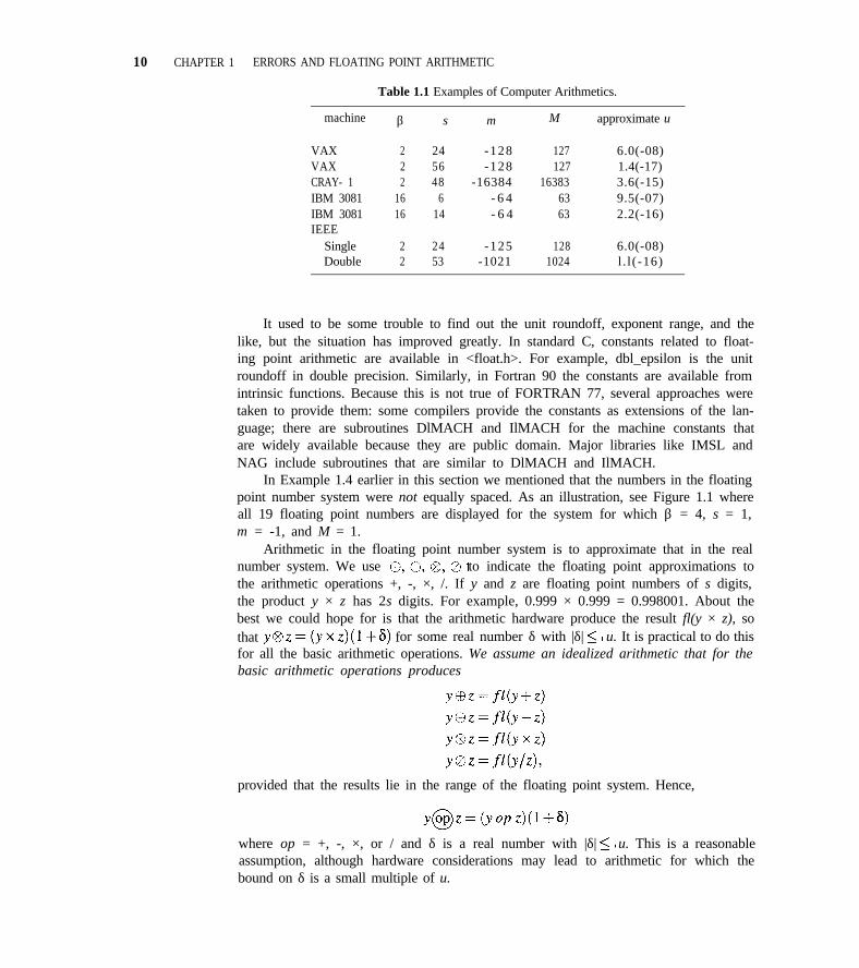
10 CHAPTER 1 ERRORS AND FLOATING POINT ARITHMETIC
Table 1.1 Examples of Computer Arithmetics.
machine β s m M approximate u
VAX 2 24 -128 127 6.0(-08)VAX 2 56 -128 127 1.4(-17)CRAY- 1 2 48 -16384 16383 3.6(-15)IBM 3081 16 6 - 6 4 63 9.5(-07)IBM 3081 16 14 - 6 4 63 2.2(-16)IEEE
Single 2 24 -125 128 6.0(-08)Double 2 53 -1021 1024 l . l (-16)
It used to be some trouble to find out the unit roundoff, exponent range, and thelike, but the situation has improved greatly. In standard C, constants related to float-ing point arithmetic are available in <float.h>. For example, dbl_epsilon is the unitroundoff in double precision. Similarly, in Fortran 90 the constants are available fromintrinsic functions. Because this is not true of FORTRAN 77, several approaches weretaken to provide them: some compilers provide the constants as extensions of the lan-guage; there are subroutines DlMACH and IlMACH for the machine constants thatare widely available because they are public domain. Major libraries like IMSL andNAG include subroutines that are similar to DlMACH and IlMACH.
In Example 1.4 earlier in this section we mentioned that the numbers in the floatingpoint number system were not equally spaced. As an illustration, see Figure 1.1 whereall 19 floating point numbers are displayed for the system for which β = 4, s = 1,m = -1, and M = 1.
Arithmetic in the floating point number system is to approximate that in the realnumber system. We use to indicate the floating point approximations tothe arithmetic operations +, -, ×, /. If y and z are floating point numbers of s digits,the product y × z has 2s digits. For example, 0.999 × 0.999 = 0.998001. About thebest we could hope for is that the arithmetic hardware produce the result fl(y × z), sothat for some real number δ with |δ| u. It is practical to do thisfor all the basic arithmetic operations. We assume an idealized arithmetic that for thebasic arithmetic operations produces
provided that the results lie in the range of the floating point system. Hence,
where op = +, -, ×, or / and δ is a real number with |δ| u. This is a reasonableassumption, although hardware considerations may lead to arithmetic for which thebound on δ is a small multiple of u.
1.1 BASIC CONCEPTS 11
Figure 1.1 Distribution of floating point numbers for β = 4, s = 1, m = -1, M = 1.
To carry out computations in this model arithmetic by hand, for each operation+, -, ×, /, perform the operation in exact arithmetic, normalize the result, and round(chop) it to the allotted number of digits. Put differently, for each operation, calculatethe result and convert i t to the machine representation before going on to the nextoperation.
Because of increasingly sophisticated architectures, the unit roundoff as definedin (1.4) is simplistic.For example, many computers do intermediate computationswith more than s digits. They have at least one “guard digit,” perhaps several, and asa consequence results can be rather more accurate than expected. (When ari thmeticoperations are carried out with more than s digits, apparently harmless actions l ikeprinting out intermediate results can cause the final result of a computation to change!This happens when the extra digits are shed as numbers are moved from arithmeticunits to storage or output devices.) It is interesting to compute (1 + δ) -1 for decreas-ing δ to see how small δ can be made and still get a nonzero result. A number of codesfor mathematical computations that are in wide use avoid defining the unit roundoffby coding a test for u|x| < h as
if ((x+h) x) then . . . .
On today’s computers this is not likely to work properly for two reasons, one being thepresence of guard digits just discussed. The other is that modern compilers defeat thetest when they “optimize” the coding by converting the test to
which is always passed.
if (h 0) then . . . ,
EXERCISES
1.1 Solve
0.461x1 + 0.311x2 = 0.150
0.209x1 + 0.141x2 = 0.068
using three-digit chopped decimal arithmetic. The ex-act answer is x1 = 1, x2 = -1; how does yours com-pare?
1.2 The following algorithm (due to Cleve Moler) esti-
mates the unit roundoff u by a computable quantityU:
A := 4./3B := A -1C := B+B+BU := |C - 1.|
(a) What does the above algorithm yield for U in six-digit decimal rounded arithmetic?
12 CHAPTER 1 ERRORS AND FLOATING POINT ARITHMETIC
(b) What does it yield for U in six-digit decimalchopped arithmetic?
(c) What are the exact values from (1.4) for u in thearithmetics of (a) and (b)?
(d) Use this algorithm on the machine(s) and calcu-lator(s) you are likely to use. What do you get?
1.3 Consider the following algorithm for generating noisein a quantity x:
A := 10n * x
B : = A + x
y : = B - A
(a) Calculate y when x = 0.123456 and n = 3 usingsix-digit decimal chopped arithmetic. What is the er-ror x - y?
(b) Repeat (a) for n = 5.
1.4 Show that the evaluation of F(x) = cosx is well-conditioned near x = 0; that is, for |x| showthat the magnitude of the relative error | [F(x) -F(0)] /F(0) | is bounded by a quantity that is not large.
1.5 If F(x) = (x - 1)2, what is the exact formula for[F(x + εx) - F(x)]/F(x)? What does this say aboutthe conditioning of the evaluation of F(x) near x = l?
1.6 Let Sn := sinxdx and show that two inte-grations by parts results in the recursion
Further argue that S0 = 2 and that Sn-1 > Sn > 0 forevery n.
(a) Compute Sl5 with this recursion (make sure thatyou use an accurate value for π).
(b) To analyze what happened in (a), consider the re-cursion
with = 2( 1 - u), that is, the same computation withthe starting value perturbed by one digit in the lastplace. Find a recursion for Sn - . From this recur-sion, derive a formula for in terms ofUse this formula to explain what happened in (a).
(c) Examine the “backwards” recursion
starting with = 0. What is Why?
1.7 For brevity let us write s = sin(θ), c = cos(θ) for somevalue of θ. Once c is computed, we can compute sinexpensively from s = (Either sign of thesquare root may be needed in general, but let us con-sider here only the positive root.) Suppose the cosineroutine produces c + δc instead of c. Ignoring any er-ror made in evaluating the formula for s, show that thisabsolute error of δc induces an absolute error in s of δswith For the range 0 /2, arethere θ for which this way of computing sin(θ) has anaccuracy comparable to the accuracy of cos(θ)? Arethere θ for which it is much less accurate? Repeat forrelative errors.
1.2 EXAMPLES OF FLOATING POINT CALCULATIONS
The floating point number system has properties that are similar to those of the realnumber system, but they are not identical. We have already seen some differencesdue to the finite range of exponents. It might be thought that because one arithmeticoperation can be carried out with small relative error, the same would be true of severaloperations. Unfortunately this is not true. We shall see that multiplication and divisionare more satisfactory in this respect than addition and subtraction.
For floating point numbers x, y and z,
1.2 EXAMPLES OF FLOATING POINT CALCULATIONS 13
The product
(1 + δ1)(l + δ2) = 1 + ε,
where ε is “small,” and can, of course, be explicitly bounded in terms of u. It is moreilluminating to note that
( 1 + δ1 )( 1 + δ2 ) = 1+ δ1 + δ2+ δ1 δ2 1 + δ 1 + δ 2 ,
so that
and an approximate bound for ε is 2u. Before generalizing this, we observe that it maywell be the case that
even when the exponent range is not exceeded. However,
so that
where η is “small.” Thus, the associative law for multiplication is approximately true.In general, if we wish to multiply xl ,x2 , . . . ,xn, we might do this by the algorithm
Pl = xl
Pi = Pi-1 x i , i = 2, 3 ,... ,n.
Treating these operations in real arithmetic we find that
Pi = xlx2···xi(l + δ1)(1 + δ2)···(1 + δι),
where each The relative error of each Pi can be bounded in terms of u withoutdifficulty, but more insight is obtained if we approximate
Pi xIx2 ···xi(l + δ1 + δ2 + · · · + δι),
which comes from neglecting products of the δι. Then
| δ1 + δ2 + ··· + δι | iu.
This says that a bound on the approximate relative errors grows additively. Each mul-tiplication could increase the relative error by no more than one unit of roundoff. Di-vision can be analyzed in the same way, and the same conclusion is true concerningthe possible growth of the relative error.
Example 1.10. The gamma function, defined as
14 CHAPTER 1 ERRORS AND FLOATING POINT ARITHMETIC
generalizes the factorial function for integers to real numbers x (and complex x aswell). This follows from the fundamental recursion
(1.5)
and the fact that (1) = 1. A standard way of approximating (x) for x 2 uses thefundamental recursion to reduce the task to approximating (y) for 2 < y < 3. Thisis done by letting N be an integer such that N < x < N + 1, letting y = x - N + 2, andthen noting that repeated applications of (1.5) yield
The function I’(y) can be approximated well by the ratio R(y) of two polynomials for2 < y < 3. Hence, we approximate
If x is not too large, little accuracy is lost when these multiplications are performed infloating point arithmetic. However, it is not possible to evaluate (x) for large x bythis approach because its value grows very quickly as a function of x. This can be seenfrom the Stirling formula (see Case Study 5)
This example makes another point: the virtue of floating point arithmetic is that itautomatically deals with numbers of greatly different size. Unfortunately, many of thespecial functions of mathematical physics grow or decay extremely fast. It is by nomeans unusual that the exponent range is exceeded. When this happens it is necessaryto reformulate the problem to make it better scaled. For example, it is often better towork with the special function ln than with I’(x) because it is better scaled. n
Addition and subtraction are much less satisfactory in floating point arithmeticthan are multiplication and division. It is necessary to be alert for several situationsthat will be illustrated. When numbers of greatly different magnitudes are added (orsubtracted), some information is lost. Suppose, for example, that we want to addδ = 0.123456 × 10⁻⁴ to 0.100000 × 101 in six-digit chopped arithmetic. First, theexponents are adjusted to be the same and then the numbers are added:
0.100000 × 101
+ 0.0000123456 ×101
0.1000123456 ×101.
The result is chopped to 0.100012 × 101. Notice that some of the digits did not par-ticipate in the addition. Indeed, if |y| < |x|u, then x y = x and the “small” number yplays no role at all. The loss of information does not mean the answer is inaccurate;it is accurate to one unit of roundoff. The problem is that the lost information may beneeded for later calculations.
1.2 EXAMPLES OF FLOATING POINT CALCULATIONS 15
Example 1.11. Difference quotients. Earlier we made use of the fact that for small
In many applications this is used to approximate F'(x). To get an accurate approxima-tion, δ must be “small” compared to x. It had better not be too small for the precision,or else we would have and compute a value of zero for F'(x). If δ is largeenough to affect the sum but still “small,” some of its digits will not affect the sum inthe sense that In the difference quotient we want to divide by the actualdifference of the arguments, not δ itself. A better way to proceed is to define
and approximate
The two approximations are mathematically equivalent, but computationally different.For example, suppose that F(x) = x and we approximate F'(x) for x = 1 using δ =0.123456 × 10⁻⁴ in six-digit chopped arithmetic. We have just worked out 1 δ =0.100012 × 101; similarly, = 0.120000 × 10⁻⁴ showing the digits of δ that actuallyaffect the sum. The first formula has
The second has
Obviously the second form provides a better approximation to F'(1) = 1. Qualitycodes for the numerical approximation of the Jacobian matrices needed for optimiza-tion, root solving, and the solution of stiff differential equations make use of this sim-ple device. n
Example 1.12. Limiting precision. In many of the codes in this book we attempt torecognize when we cannot achieve a desired accuracy with the precision available. Thekind of test we make will be illustrated in terms of approximating a definite integral
This might be done by splitting the integration interval [a,b] into pieces [α,β] andadding up approximations on all the pieces. Suppose that
The accuracy of this formula improves as the length β - α of the piece is reduced, sothat, mathematically, any accuracy can be obtained by making this width sufficiently
16 CHAPTER 1 ERRORS AND FLOATING POINT ARITHMETIC
small. However, if |β - α| < 2u |α|, the floating point numbers a and a + (β - α)/2are the same. The details of the test are not important for this chapter; the point is thatwhen the interval is small enough, we cannot ignore the fact that there are only a finitenumber of digits in floating point arithmetic. If a and β cannot be distinguished in theprecision available, the computational results will not behave like mathematical resultsfrom the real number system. In this case the user of the software must be warned thatthe requested accuracy is not feasible. n
Example I. 13. Summing a divergent series. The sum S of a series
is the limit of partial sums
There is an obvious algorithm for evaluating S:
S1 = a1
Sn = Sn-1 an, n = 2, 3,...,
continuing until the partial sums stop changing. A classic example of a divergent seriesis the harmonic series
If the above algorithm is applied to the harmonic series, the computed Sn increase andthe a, decrease until
and the partial sums stop changing. The surprising thing is how small Sn is when thishappens-try it and see. In floating point arithmetic this divergent series has a finitesum. The observation that when the terms become small enough, the partial sumsstop changing is true of convergent as well as divergent series. Whether the value soobtained is an accurate approximation to S depends on how fast the series converges.It really is necessary to do some mathematical analysis to get reliable results. Later inthis chapter we consider how to sum the terms a little more accurately. n
An acute difficulty with addition and subtraction occurs when some information,lost due to adding numbers of greatly different size, is needed later because of a sub-traction. Before going into this, we need to discuss a rather tricky point.
Example 1.14. Cancellation (loss of significance). Subtracting a number y from anumber x that agrees with it in one or more leading digits leads to a cancellation of
1.2 EXAMPLES OF FLOATING POINT CALCULATIONS 17
these digits. For example, if x = 0.123654 × 10⁻⁵ and y = 0.123456 × 10⁻⁵, then
0.123654 × 10⁻⁵
– 0.123456 × 10⁻⁵
0.000198 × 10-5 = 0.198000 × 10⁻⁸.
The interesting point is that when cancellation takes place, the subtraction is doneexactly, so that x y = x - y. The difficulty is what is called a loss of significance.When cancellation takes place, the result x - y is smaller in size than x and y, soerrors already present in x and y are relatively larger in x - y. Suppose that x is anapproximation to X and y is an approximation to Y. They might be measured values orthe results of some computations. The difference x - y is an approximation to X - Ywith the magnitude of its relative error satisfying
If x is so close to y that there is cancellation, the relative error can be large be-cause the denominator X - Y is small compared to X or Y. For example, if X =0.123654700 ··· × 10-5, then x agrees with X to a unit roundoff in six-digit arithmetic.With Y = y the value we seek is X - Y = 0.198700 ··· × 10-8. Even though the sub-traction x - y = 0.198000 × 10⁻⁸ is done exactly, x - y and X - Y differ in the fourthdigit. In this example, x and y have at least six significant digits, but their differencehas only three significant digits. n
It is worth remarking that we made use of cancellation in Example 1.11 when wecomputed
Because δ is small compared to x, there is cancellation and In thisway we obtain in A the digits of δ that actually affected the sum.
Example 1.15. Roots of a quadratic. Suppose we wish to compute the roots of
x 2 + b x + c = 0 .
The familiar quadratic formula gives the roots xl and x2 as
assuming b > 0. If c is small compared to b, the square root can be rewritten andapproximated using the binomial series to obtain
18 CHAPTER 1 ERRORS AND FLOATING POINT ARITHMETIC
This shows that the true roots
x1 -bx2 -c/b.
In finite precision arithmetic some of the digits of c have no effect on the sum (b/2)2 -c. The extreme case is
It is important to appreciate that the quantity is computed accurately in a relative sense.However, some information is lost and we shall see that in some circumstances weneed it later in the computation. A square root is computed with a small relativeerror and the same is true of the subtraction that follows. Consequently, the biggerroot xl -b is computed accurately by the quadratic formula. In the computationof the smaller root, there is cancellation when the square root term is subtracted from-b/2. The subtraction itself is done exactly, but the error already present in (b/2)2 cbecomes important in a relative sense. In the extreme case the formula results in zeroas an approximation to x2.
For this particular task a reformulation of the problem avoids the difficulty. Theexpression
( x-x1)( x-x2) = x2 - (xl + x2) + x1x2
= x2+ bx + c
shows that x1x2 = c. As we have seen, the bigger root xl can be computed accuratelyusing the quadratic formula and then
x2 = c/xl
provides an accurate value for x2. n
Example 1.16. Alternating series. As we observed earlier, it is important to knowwhen enough terms have been taken from a series to approximate the limit to a desiredaccuracy. Alternating series are attractive in this regard. Suppose a0 > al > ··· > an> an+ 1 > ··· > 0 and = 0. Then the alternating series
converges to a limit S and the error of the partial sum
satisfies
|S-S n | < a n+1·
To see a specific example, consider the evaluation of sinx by its Maclaurin series
1.2 EXAMPLES OF FLOATING POINT CALCULATIONS 19
Although this series converges quickly for anywhen |x| is large. If, say, x = 10, the am are
given x, there are numerical difficulties
Clearly there are some fairly large terms here that must cancel out to yield a resultsin 10 that has magnitude at most 1. The terms am are the result of some computationthat here can be obtained with small relative error. However, if am is large comparedto the sum S, a small relative error in am will not be small compared to S and S willnot be computed accurately.
We programmed the evaluation of this series in a straightforward way, being care-ful to compute, say,
so as to avoid unnecessarily large quantities. Using single precision standard IEEEarithmetic we added terms until the partial sums stopped changing. This produced thevalue -0.544040 while the exact value should be sinx = -0.544021. Although theseries converges quickly for all x, some intermediate terms become large when |x| islarge. Indeed, we got an overflow due to the small exponent range in IEEE singleprecision arithmetic when we tried x = 100. Clearly floating point arithmetic does notfree us from all concerns about scaling.
Series are often used as a way of evaluating functions. If the desired functionvalue is small and if some terms in the series are comparatively large, then there mustbe cancellation and we must expect that inaccuracies in the computation of the termswill cause the function value to be inaccurate in a relative sense. n
We have seen examples showing that the sum of several numbers depends on theorder in which they are added. Is there a “good” order? We now derive a rule of thumbthat can be quite useful. We can form a1 + a2 + ··· + aN by the algorithm used inExample 1.13. The first computed partial sum is
where |δ2| < u. It is a little special. Thecomputed partial sum, which is
general case is represented by the next
where |δ3| < u. To gain insight, we approximate this expression by dropping termsinvolving the products of small factors so that
20 CHAPTER 1 ERRORS AND FLOATING POINT ARITHMETIC
Continuing in this manner we find that
According to this approximation, the error made when ak is added to Sk might grow,but its effect in S, will be no bigger than (N - k + l) u|ak|. This suggests that toreduce the total error, the terms should be added in order of increasing magnitude. Acareful bound on the error of repeated summation leads to the same rule of thumb.Adding in order of increasing magnitude is usually a good order, but not necessarilya good order (because of the complex ways that the individual errors can interact).Much mathematical software makes use of this device to enhance the accuracy of thecomputations.
The approximate error can be bounded by
Here we use the symbol to mean “less than or equal to a quantity that is approxi-mately.” (The “less than” is not sharp here.) Further manipulation provides an approx-imate bound on the magnitude of the sum’s relative error
The dangerous situation is when which is when cancellationtakes place. An important consequence is that if all the terms have the same sign, thesum will be computed accurately in a relative sense, provided only that the number ofterms is not too large for the precision available.
For a convergent series
it is necessary that Rather than sum in the natural order m =
0, 1,..., it would often be better to work out mathematically how many terms N areneeded to approximate S to the desired accuracy and then calculate SN in the reverseorder aN, aN-1,....
Example 1.17. There are two ways of interpreting errors that are important in nu-merical analysis. So far we have been considering a forward error analysis. Thiscorresponds to bounding the errors in the answer by bounding at each stage the errorsthat might arise and their effects. To be specific, recall the expression for the error ofsumming three numbers:
1.2 EXAMPLES OF FLOATING POINT CALCULATIONS 21
A forward error analysis might bound the absolute error by
(This is a sharp version of the approximate bound given earlier.) A backward erroranalysis views the computed result as the result computed in exact arithmetic of aproblem with somewhat different data. Let us reinterpret the expression for fl( S 3) inthis light. It is seen that
f l( S 3) = y l + y 2 + y 3 ,
where
In the backward error analysis view, the computed sum is the exact sum of terms yk
that are each close in a relative sense to the given data xk. An algorithm that is stablein the sense of backward error analysis provides the exact solution of a problem withdata close to that of the original problem. As to whether the two solutions are close,that is a matter of the conditioning of the problem. A virtue of this way of viewingerrors is that it separates the roles of the stability of the algorithm and the conditionof the problem. Backward error analysis is particularly attractive when the input dataare of limited accuracy, as, for example, when the data are measured or computed. Itmay well happen that a stable algorithm provides the exact solution to a problem withdata that cannot be distinguished from the given data because of their limited accuracy.We really cannot ask more of the numerical scheme in such a situation, but again wemust emphasize that how close the solution is to that corresponding to the given datadepends on the conditioning of the problem. We shall return to this matter in the nextchapter.
A numerical example will help make the point. For xl = 0.12 × 10², x2 = 0.34 ×101, x3 = -0.15 × 10², the true value of the sum is S3 = 0.40 × 100. When evaluatedin two digit decimal chopped arithmetic, fl (S3) = 0.00 × 100, a very inaccurate result.Nevertheless, with y1 = 0.116 × 10², y2 = x2, and y3 = x3, we have fl(S3) = y1+ y2 +y3. The computed result is the exact sum of numbers close to the original data. Indeed,two of the numbers are the same as the original data and the remaining one differs byless than a unit of roundoff. n
For most of the numerical tasks in this book it is not necessary to worry greatlyabout the effects of finite precision arithmetic. Two exceptions are the subject of theremaining examples. The first is the computation of a root of a continuous functionf(x). Naturally we would like to compute a number z for which f(z) is as close tozero as possible in the precision available. Routines for this purpose ask the user tospecify a desired accuracy. Even if the user does not request a very accurate root, theroutine may “accidentally” produce a number z for which f(z) is very small. Becauseit is usually not expensive to solve this kind of problem, it is quite reasonable for a user
22 CHAPTER 1 ERRORS AND FLOATING POINT ARITHMETIC
to ask for all the accuracy possible. One way or the other, we must ask what happens
when x is very close to a root. An underflow is possible since I fthis does not happen, it is usually found that the value of f(z) fluctuates erratically as
Because of this we must devise algorithms that will behave sensibly when thecomputed value f(x) does not have even the correct sign for x near z. An example willshow how the details of evaluation of f(x) are important when x is near a root.
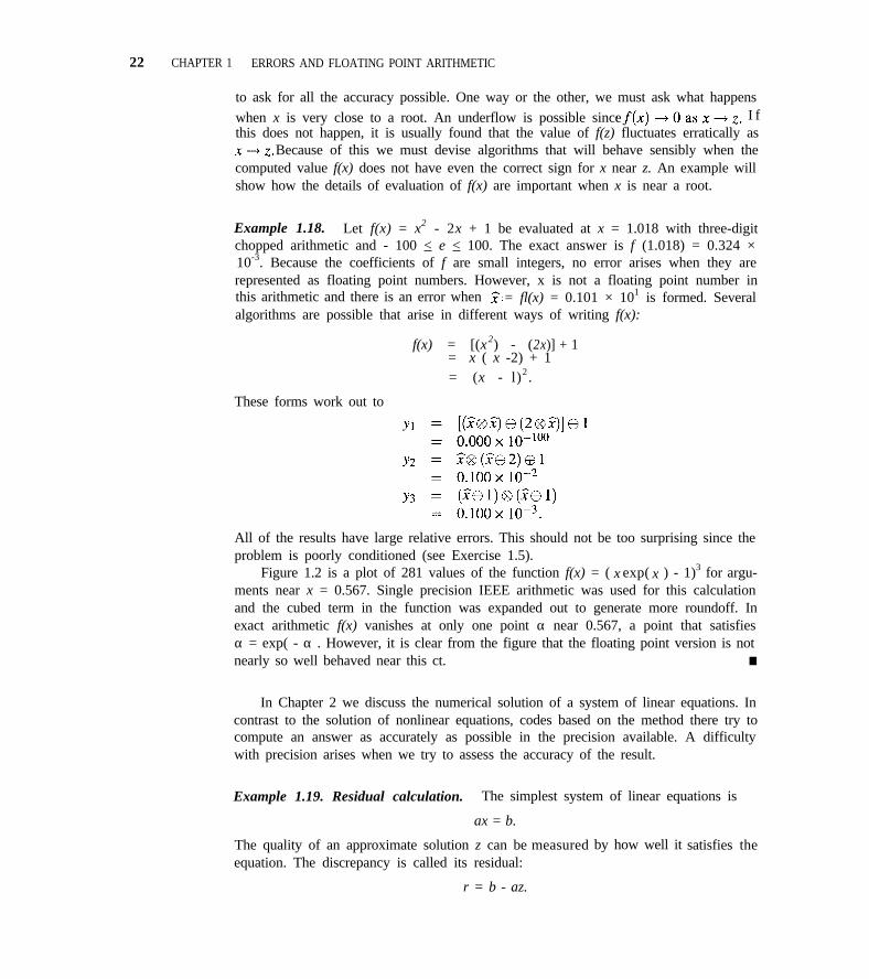
Example 1.18. Let f(x) = x2 - 2x + 1 be evaluated at x = 1.018 with three-digitchopped arithmetic and - 100 < e < 100. The exact answer is f (1.018) = 0.324 ×10⁻³. Because the coefficients of f are small integers, no error arises when they arerepresented as floating point numbers. However, x is not a floating point number inthis arithmetic and there is an error when = fl(x) = 0.101 × 101 is formed. Severalalgorithms are possible that arise in different ways of writing f(x):
f(x) = [(x2) - (2x)] + 1= x ( x -2) + 1= (x - l)2 .
These forms work out to
All of the results have large relative errors. This should not be too surprising since theproblem is poorly conditioned (see Exercise 1.5).
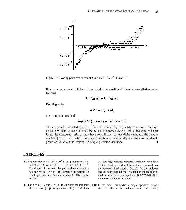
Figure 1.2 is a plot of 281 values of the function f(x) = ( x exp( x ) - 1)3 for argu-ments near x = 0.567. Single precision IEEE arithmetic was used for this calculationand the cubed term in the function was expanded out to generate more roundoff. Inexact arithmetic f(x) vanishes at only one point α near 0.567, a point that satisfiesα = exp( - α). However, it is clear from the figure that the floating point version is notnearly so well behaved near this ct. n
In Chapter 2 we discuss the numerical solution of a system of linear equations. Incontrast to the solution of nonlinear equations, codes based on the method there try tocompute an answer as accurately as possible in the precision available. A difficultywith precision arises when we try to assess the accuracy of the result.
Example 1.19. Residual calculation. The simplest system of linear equations is
ax = b.
The quality of an approximate solution z can beequation. The discrepancy is called its residual:
r = b - az.
measured by how well it satisfies the
1.2 EXAMPLES OF FLOATING POINT CALCULATIONS 23
Figure 1.2 Floating point evaluation of f(x) = x3e3x - 3x2 e2x + 3xex - 1.
If z is a very good solution, its residual r is small and there is cancellation whenforming
Defining δ by
the computed residual
The computed residual differs from the true residual by a quantity that can be as largeas |az|u |b|u. When r is small because z is a good solution and |b| happens to be enlarge, the computed residual may have few, if any, correct digits (although the relativeresidual |r/b| is fine). When z is a good solution, it is generally necessary to use doubleprecision to obtain its residual to single precision accuracy. n
EXERCISES
1.8 Suppose that z = 0.180 × 10² is an approximate solu- use four-digit decimal chopped arithmetic, then four-tion of ax = b for a = 0.111 × 100, b = 0.200 × 101. digit decimal rounded arithmetic. How reasonable areUse three-digit decimal chopped arithmetic to com- the answers? Find another formula for the midpointpute the residual r = b - az. Compute the residual in and use four-digit decimal (rounded or chopped) arith-double precision and in exact arithmetic. Discuss the metic to calculate the midpoint of [0.8717,0.8719]. Isresults. your formula better or worse?
1.9 For α = 0.8717 and β = 0.8719 calculate the midpoint 1.10 In the model arithmetic, a single operation is car-of the interval [α, β] using the formula (α+ β)/2. First ried out with a small relative error. Unfortunately
24 CHAPTER 1 ERRORS AND FLOATING POINT ARITHMETIC
the same is not true of complex arithmetic. To seethis, let z = a + ib and w = c + id. By definition,zw = (ac - bd) + i(ad + bc). Show how the real part,ac - bd, of the product zw might be computed with alarge relative error even though all individual calcula-tions are done with a small relative error.
1.11 An approximation S to ex can be computed by usingthe Taylor series for the exponential function:
S := 1P := 1for k = 1,2,...begin
P := xP/kS := S+P
end k.The loop can be stopped when S = S + P to machineprecision.
(a) Try this algorithm with x = - 10 using single pre-cision arithmetic. What was k when you stopped?What is the relative error in the resulting approxima-tion? Does this appear to be a good way to computee -10 to full machine precision?
(b) Repeat (a) with x = + 10.
(c) Why are the results so much more reasonable for
(b)?(d) What would be a computationally safe way tocompute e-10?
1.12 Many problems in astrodynamics can be approxi-mated by the motion of one body about another underthe influence of gravity, for example, the motion of asatellite about the earth. This is a useful approxima-tion because by a combination of analytical and nu-merical techniques, these two body problems can besolved easily. When a better approximation is desired,for example, we need to account for the effect of themoon or sun on the satellite, it is natural to compute itas a correction to the orbit of the two body problem.This is the basis of Encke’s method; for details seeSection 9.3 of [2]. A fundamental issue is to calculateaccurately the small correction to the orbit. This isreduced to the accurate calculation of a function f(q)for small q > 0. The function is
Explain why f(q) cannot be evaluated accurately infinite precision arithmetic when q is small. In the ex-planation you should assume that y-3/2 can be eval-uated with a relative error that is bounded by a smallmultiple of the unit roundoff. Use the binomial seriesto show
Why is this series a better way to evaluate f(q) whenq is small?
1.13 Let a regular polygon of N sides be inscribed in a unitcircle. If LN denotes the length of one side, the cir-cumference of the polygon, N × LN, approximates thecircumference of the circle, 2π; hence π: NLN/2 forlarge N. Using Pythagoras’ theorem it is easy to relateL2N to LN:
Starting with L4 = for a square, approximate πby means of this recurrence. Explain why a straight-forward implementation of the recurrence in floatingpoint arithmetic does not yield an accurate value forπ. (Keep in mind that Show thatthe recurrence can be rearranged as
and demonstrate that this form works better.
1.14 A study of the viscous decay of a line vortex leads toan expression for the velocity
at a distance r from the origin at time t > 0. Hereis the initial circulation and v > 0 is the kinematic vis-cosity. For some purposes the behavior of the velocityat distances r << is of particular interest. Whyis the form given for the velocity numerically unsat-isfactory for such distances? Assuming that you haveavailable a function for the accurate computation ofsinh( x ), manipulate the expression into one that canbe evaluated in a more accurate way for very small r.
1.3 CASESTUDY 1 25
1.3 CASE STUDY 1
Now let us look at a couple of examples that illustrate points made in this chapter. Thefirst considers the evaluation of a special function. The second illustrates the fact thatpractical computation often requires tools from several chapters of this book. Filon’smethod for approximating finite Fourier integrals will be developed in Chapter 3 andapplied in Chapter 5. An aspect of the method that we take up here is the accuratecomputation of coefficients for the method.
The representation of the hyperbolic cosine function in terms of exponentials
x = cosh(y) = exp( y) + exp(-y)2
makes it easy to verify that for x > 1,
Let us consider the evaluation of this expression for cosh-1 (x) in floating point arith-metic when x >> 1. An approximation made earlier in this chapter will help us tounderstand better what it is that we want to compute. After approximating
we find that
The first difficulty we encounter in the evaluation is that when x is very large, x2 over-flows. This overflow is unnecessary because the argument we are trying to compute ison scale. If x is large, but not so large that x2 overflows, the effect of the 1 “falls off theend” in the subtraction, meaning that fl(x2 - 1) = fl(x2). This subtraction is carriedout with a small relative error, and the same is true of less extreme cases, but there isa loss of information when numbers are of greatly different size. The square root isobtained with a small relative error. The information lost in the subtraction is neededat the next step because there is severe cancellation. Indeed, for large x, we might endup computing x - x = 0 as the argument for ln(x), which would be disastrous.
How might we reformulate the task to avoid the difficulties just noted? A littlecalculation shows that
a form that avoids cancellation. The preliminary analysis we did to gain insight sug-gests a better way of handling the rest of the argument:
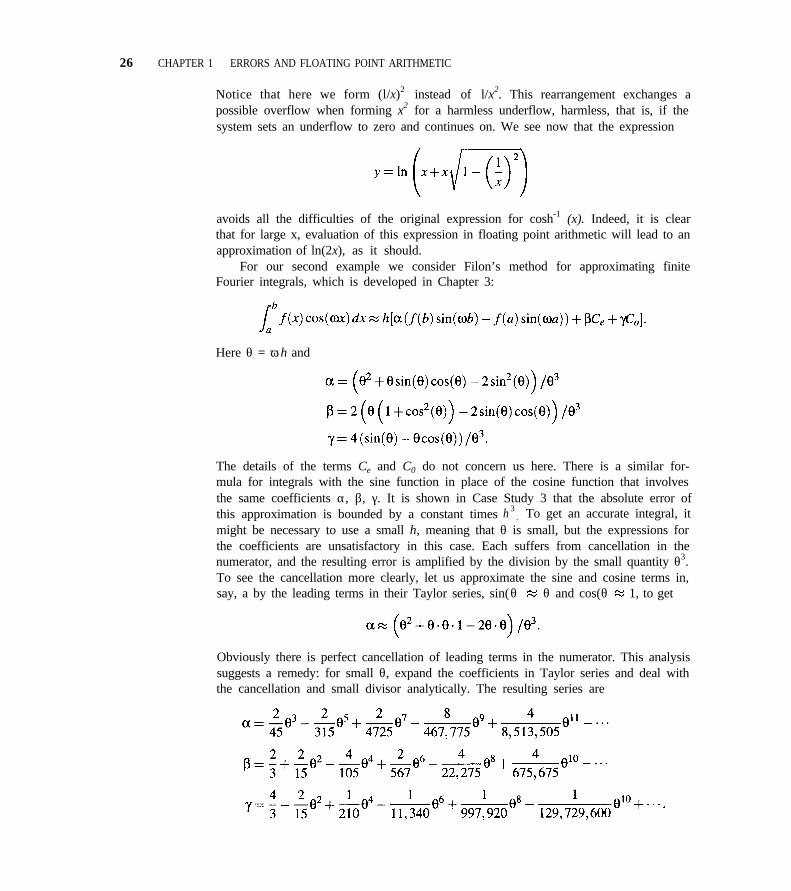
26 CHAPTER 1 ERRORS AND FLOATING POINT ARITHMETIC
Notice that here we form (l/x)2 instead of l/x2. This rearrangement exchanges apossible overflow when forming x2 for a harmless underflow, harmless, that is, if thesystem sets an underflow to zero and continues on. We see now that the expression
avoids all the difficulties of the original expression for cosh-1 (x). Indeed, it is clearthat for large x, evaluation of this expression in floating point arithmetic will lead to anapproximation of ln(2x), as it should.
For our second example we consider Filon’s method for approximating finiteFourier integrals, which is developed in Chapter 3:
Here θ = ωh and
The details of the terms Ce and C0 do not concern us here. There is a similar for-mula for integrals with the sine function in place of the cosine function that involvesthe same coefficients α, β, γ. It is shown in Case Study 3 that the absolute error ofthis approximation is bounded by a constant times h 3
. To get an accurate integral, itmight be necessary to use a small h, meaning that θ is small, but the expressions forthe coefficients are unsatisfactory in this case. Each suffers from cancellation in thenumerator, and the resulting error is amplified by the division by the small quantity θ3.To see the cancellation more clearly, let us approximate the sine and cosine terms in,say, a by the leading terms in their Taylor series, sin(θ) θ and cos(θ) 1, to get
Obviously there is perfect cancellation of leading terms in the numerator. This analysissuggests a remedy: for small θ, expand the coefficients in Taylor series and deal withthe cancellation and small divisor analytically. The resulting series are
1.3 CASE STUDY 1 27
It might be remarked that it was easy to compute these expansions by means of thesymbolic capabilities of the Student Edition of MATLAB. In the program used to com-pute the integral of Case Study 3, these expressions were used for θ < 0.1. Because theterms decrease rapidly, nested multiplication is not only an efficient way to evaluatethe expressions but is also accurate.
As a numerical illustration of the difficulty we evaluated both forms of a for arange of θ in single precision in FORTRAN. Reference values were computed usingthe trigonometric form and double precision. This must be done with some care. Forinstance, if T is a single precision variable and we want a double precision copy DTfor computing the reference values, the lines of code
T = 0.lE0DT = 0. 1D0
are not equivalent to
T = 0.1E0D T = T
This is because on a machine with binary or hexadecimal arithmetic, 0. 1E0 agrees with0.1 D0 only to single precision. For the reference computation we require a double pre-cision version of the actual machine number used in the single precision computations,hence we must use the second code. As we have remarked previously, most computerstoday perform intermediate computations in higher precision, despite specification ofthe precision of all quantities. With T, S, and C declared as single precision variables,we found remarkable differences in the result of
S = SIN(T)C = COS(T)ALPHA=(T**2+T*S*C-2EO*S**2)/T**3
and
ALPHA=(T**2+T*SIN(T)*COS(T)-2EO*SIN(T)**2)/T**3
differences that depended on the machine and compiler used. On a PC with a Pentiumchip, the second code gave nearly full single precision accuracy. The first gave thepoor results that we expect of computations carried out entirely in single precision.
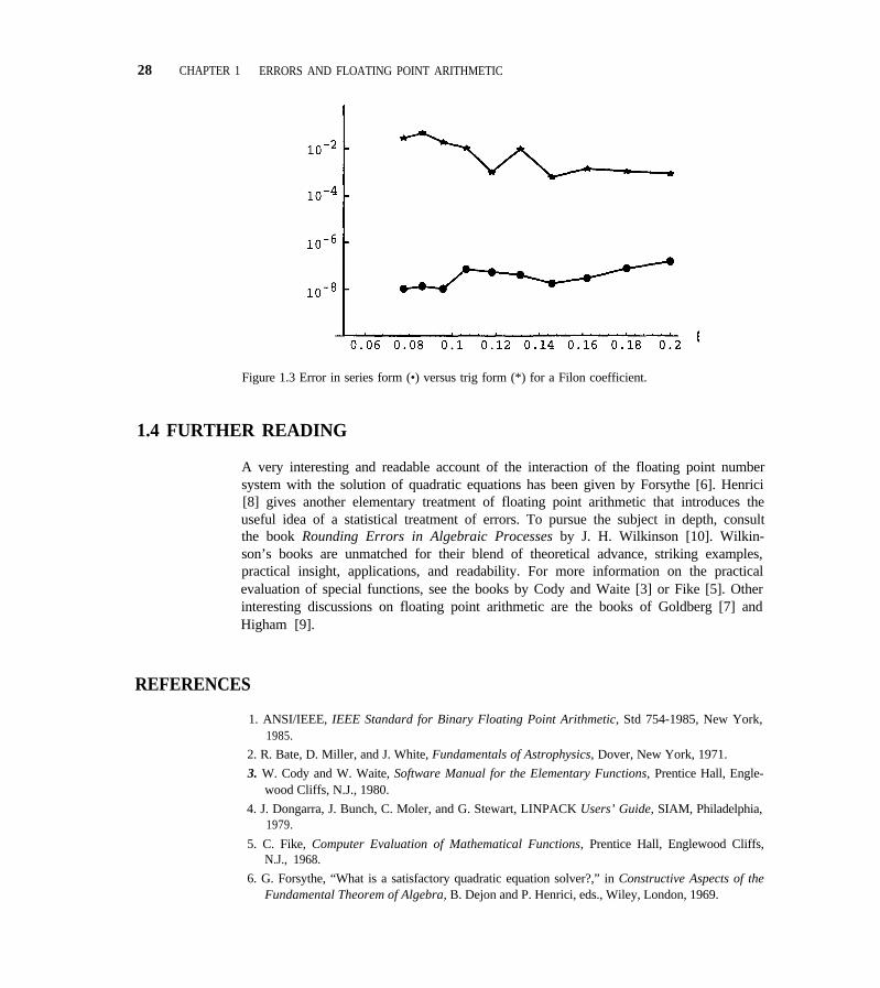
The coefficient a was computed for a range of θ using the trigonometric defini-tion and single precision arithmetic and its relative error computed using a referencevalue computed in double precision. Similarly the error of the value computed in sin-gle precision from the Taylor series was found. Plotted against θ in Figure 1.3 is therelative error for both methods (on a logarithmic scale). Single precision accuracycorresponds to about seven digits, so the Taylor series approach gives about all theaccuracy we could hope for, although for the largest value of θ it appears that anotherterm in the expansion would be needed to get full accuracy. Obviously the trigono-metric definition leads to a great loss of accuracy for “small” θ. Indeed, θ is not verysmall in an absolute sense here; rather, it is small considering its implications for thecost of evaluating the integral when the parameter ω is moderately large.
28 CHAPTER 1 ERRORS AND FLOATING POINT ARITHMETIC
Figure 1.3 Error in series form (•) versus trig form (*) for a Filon coefficient.
1.4 FURTHER READING
A very interesting and readable account of the interaction of the floating point numbersystem with the solution of quadratic equations has been given by Forsythe [6]. Henrici[8] gives another elementary treatment of floating point arithmetic that introduces theuseful idea of a statistical treatment of errors. To pursue the subject in depth, consultthe book Rounding Errors in Algebraic Processes by J. H. Wilkinson [10]. Wilkin-son’s books are unmatched for their blend of theoretical advance, striking examples,practical insight, applications, and readability. For more information on the practicalevaluation of special functions, see the books by Cody and Waite [3] or Fike [5]. Otherinteresting discussions on floating point arithmetic are the books of Goldberg [7] andHigham [9].
REFERENCES
1. ANSI/IEEE, IEEE Standard for Binary Floating Point Arithmetic, Std 754-1985, New York,1985.
2. R. Bate, D. Miller, and J. White, Fundamentals of Astrophysics, Dover, New York, 1971.
3. W. Cody and W. Waite, Software Manual for the Elementary Functions, Prentice Hall, Engle-wood Cliffs, N.J., 1980.
4. J. Dongarra, J. Bunch, C. Moler, and G. Stewart, LINPACK Users’ Guide, SIAM, Philadelphia,1979.
5. C. Fike, Computer Evaluation of Mathematical Functions, Prentice Hall, Englewood Cliffs,N.J., 1968.
6. G. Forsythe, “What is a satisfactory quadratic equation solver?,” in Constructive Aspects of theFundamental Theorem of Algebra, B. Dejon and P. Henrici, eds., Wiley, London, 1969.
REFERENCES 29
7. D. Goldberg, “What every computer scientist should know about floating-point arithmetic,”ACM Computing Surveys, 23 (1991), pp. 5-48.
8. P. Henrici, Elements of Numerical Analysis, Wiley, New York, 1964.
9. N. Higham, Accuracy and Stability of Numerical Algorithms, SIAM, Philadelphia, 1996.
10. J. Wilkinson, Rounding Errors in Algebraic Processes, Dover, Mineola, N.Y., 1994.
MISCELLANEOUS EXERCISES FOR CHAPTER 1
1.15 Use three-digit decimal chopped arithmetic with m =- 100 and M = 100 to construct examples for which
You are allowed to use negative numbers. Examplescan be constructed so that either one of the expres-sions cannot be formed in the arithmetic, or both canbe formed but the values are different.
1.16 For a set of measurements xl ,x2,. . . ,xN, the samplemean is defined to be
The sample standard deviation s is defined to be
Another expression,
is often recommended for hand computation of s.Show that these two expressions for s are mathemat-ically equivalent. Explain why one of them may pro-vide better numerical results than the other, and con-struct an example to illustrate your point.
1.17 Fourier series,
are of great practical value. It appears to be necessaryto evaluate a large number of sines and cosines if wewish to evaluate such a series, but this can be donecheaply by recursion. For the specific x of interest, forn = 1, 2,...let
sn = sinnx and cn = cosnx.
Show that for n = 2, 3,. . .
sn = S1Cn-I + c1sn-l and cn = c1cn-l -s1sn-l.
After evaluating sl = sinx and c1 = cosx with the in-trinsic functions of the programming language, thisrecursion can be used to evaluate simply and inex-pensively all the sinnx and cosnx that are needed.To see that the recursion is stable, suppose that forsome m > 1, sm and cm are computed incorrectly as = sm + εm and = cm + If no further arith-metic errors are made, the errors εm and will prop-agate in the recurrence so that we compute
for n = m + l,.... Let εn and be the errors in and so that, by definition,
Prove that for all n > m
which implies that for all n > m
In this sense, errors are not amplified and the recur-rence is quite stable.
CHAPTER 2
SYSTEMS OF LINEAR EQUATIONS
One of the most frequently encountered problems in scientific computation is that ofsolving n simultaneous linear equations in n unknowns. If we denote the unknowns byx1,x2, . . . xn, such a system can be written in the form
The given data here are the right-hand sides bi, i = 1, 2,. . . , n, and the coefficients aij
for i, j = 1, 2,..., n. Problems of this nature arise almost everywhere in the applicationsof mathematics (e.g., the fitting of polynomials and other curves through data andthe approximation of differential and integral equations by finite, algebraic systems).Several specific examples are found in the exercises for this chapter (see also [12]or [13]). To talk about (2.1) conveniently, we shall on occasion use some notationfrom matrix theory. However, we do not presume that the reader has an extensivebackground in this area. Using matrices, (2.1) can be written compactly as
(2.2)
where
A x = b ,
If a11 0, the equation has a unique solution, namely x1 = b1/a11. If a11 = 0, thensome problems do not have solutions (b1 0) while others have many solutions (ifb1 = 0, any number x1 is a solution). The same is true for general n. There are twokinds of matrices, nonsingular and singular. If the matrix A is nonsingular, there is aunique solution vector x for any given right-hand side b. If A is singular, there is no
30
31
solution for some right-hand sides b and many solutions for other b. In this book weconcentrate on systems of linear equations with nonsingular matrices.
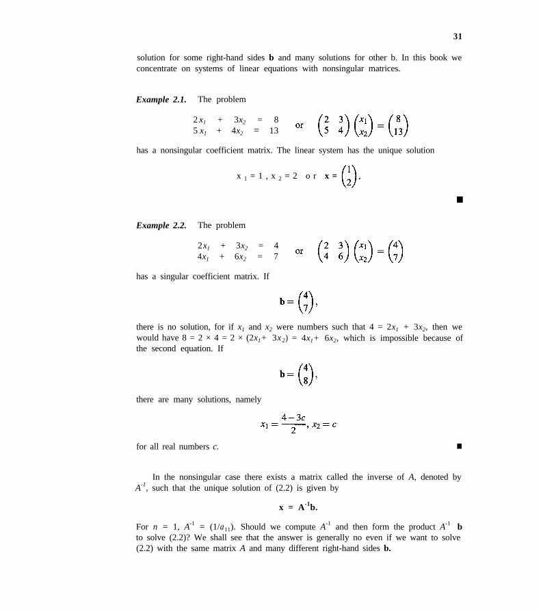
Example 2.1. The problem
2 x1 + 3x2 = 85 x1 + 4x2 = 13
has a nonsingular coefficient matrix. The linear system has the unique solution
x 1 = 1 , x 2 = 2 o r x =
Example 2.2. The problem
2x1 + 3x2 = 44x1 + 6x2 = 7
has a singular coefficient matrix. If
there is no solution, for if x1 and x2 were numbers such that 4 = 2x1 + 3x2, then wewould have 8 = 2 × 4 = 2 × (2x1+ 3x2) = 4x1+ 6x2, which is impossible because ofthe second equation. If
there are many solutions, namely
for all real numbers c. n
In the nonsingular case there exists a matrix called the inverse of A, denoted byA-1, such that the unique solution of (2.2) is given by
x = A-1b.
For n = 1, A-1 = (1/a11). Should we compute A-1 and then form the product A-1 bto solve (2.2)? We shall see that the answer is generally no even if we want to solve(2.2) with the same matrix A and many different right-hand sides b.
32 CHAPTER 2 SYSTEMS OF LINEAR EQUATIONS
2.1 GAUSSIAN ELIMINATION WITH PARTIAL PIVOTING
The most popular method for solving a nonsingular system of linear equations (2.1) iscalled Gaussian elimination. It is both simple and effective. In principle it can be usedto compute solutions of problems with singular matrices when they have solutions, butthere are better ways to do this. The basic idea in elimination is to manipulate theequations of (2.1) so as to obtain an equivalent set of equations that is easy to solve.An equivalent set of equations is one that has the same solutions. There are three basicoperations used in elimination: (1) multiplying an equation by a nonzero constant,(2) subtracting a multiple of one equation from another, and (3) interchanging rows.First, if any equation of (2.1) is multiplied by the nonzero constant a, we obtain anequivalent set of equations. To see this, suppose that we multiply the k th equation bya to get
(2.3)
If x1, x2, . . . ,xn satisfy (2.1), then they obviously satisfy the set of equations that is thesame as (2.1) except for the kth equation, which is (2.3). Conversely, because α 0,if x1, x2, . . . ,xn satisfy this second set of equations, they obviously satisfy the first.Second, suppose we replace equation i by the result of subtracting the multiple a ofequation k from equation i:
If x1, x2, . . . ,xn satisfy (2.l), then by definition
and
aklxl + ak2x2 + ··· + aknxn = bk,
so that
( ai1x1 + ai2x2 + ··· + ainxn) - α (ak1x1 + ··· + aknxn) = bi - αbk.
Thus xl, x2 , . . . ,xn satisfy all the equations of (2.4). To work in reverse, suppose nowthat x1, x2,. . . ,xn satisfy (2.4). Then in particular they satisfy equations i and k,
so that
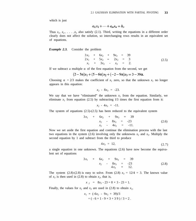
2.1 GAUSSIAN ELIMINATION WITH PARTIAL PIVOTING 33
which is just
Thus x1, x2 , . . . ,xn also satisfy (2.1). Third, writing the equations in a different orderclearly does not affect the solution, so interchanging rows results in an equivalent setof equations.
Example 2.3. Consider the problem
3 x1 + 6x2 + 9x3 = 392x1 + 5x2 - 2x3 = 3
x1 + 3x2 - x3 = 2.
If we subtract a multiple α of the first equation from the second, we get
(2.5)
Choosing α = 2/3 makes the coefficient of x1 zero, so that the unknown x1 no longerappears in this equation:
x2 - 8x3 = -23.
We say that we have “eliminated” the unknown x1 from the equation. Similarly, weeliminate x1 from equation (2.5) by subtracting l/3 times the first equation from it:
x2 - 4x3 = -11.
The system of equations (2.5)-(2.5) has been reduced to the equivalent system
3x1 + 6x2 + 9x3 = 39x2 - 8x3 = -23 (2.6)x2 - 4x3 = -11.
Now we set aside the first equation and continue the elimination process with the lasttwo equations in the system (2.6) involving only the unknowns x2 and x3. Multiply thesecond equation by 1 and subtract from the third to produce
4x3 = 12, (2.7)
a single equation in one unknown. The equations (2.6) have now become the equiva-lent set of equations
3x1 + 6x2 + 9x3 = 39x2 - 8x3 = -23 (2.8)
4 x3 = 12.
The system (2.8)-(2.8) is easy to solve. From (2.8) x3 = 12/4 = 3. The known valueof x3 is then used in (2.8) to obtain x2, that is,
x 2 = 8x3 - 23 = 8 × 3 - 23 = 1.
Finally, the values for x2 and x3 are used in (2.8) to obtain x1,
x1 = (-6x2 - 9x3 + 39)/3
= ( - 6 × 1 - 9 × 3 + 3 9 ) / 3 = 2 .
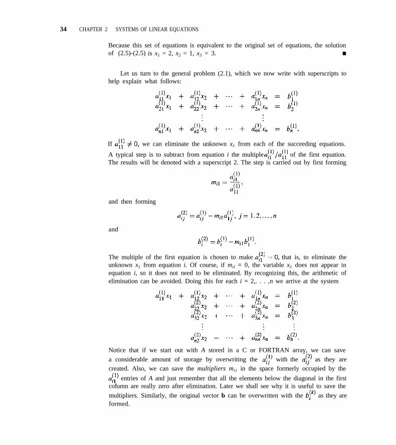
34 CHAPTER 2 SYSTEMS OF LINEAR EQUATIONS
Because this set of equations is equivalent to the original set of equations, the solutionof (2.5)-(2.5) is x1 = 2, x2 = 1, x3 = 3. n
Let us turn to the general problem (2.1), which we now write with superscripts tohelp explain what follows:
If we can eliminate the unknown x1 from each of the succeeding equations.
A typical step is to subtract from equation i the multiple of the first equation.The results will be denoted with a superscript 2. The step is carried out by first forming
and then forming
and
The multiple of the first equation is chosen to make that is, to eliminate theunknown x1 from equation i. Of course, if mil = 0, the variable x1 does not appear inequation i, so it does not need to be eliminated. By recognizing this, the arithmetic ofelimination can be avoided. Doing this for each i = 2,. . . ,n we arrive at the system
Notice that if we start out with A stored in a C or FORTRAN array, we can save
a considerable amount of storage by overwriting the with the as they arecreated. Also, we can save the multipliers mi1 in the space formerly occupied by the
entries of A and just remember that all the elements below the diagonal in the firstcolumn are really zero after elimination. Later we shall see why it is useful to save the
multipliers. Similarly, the original vector b can be overwritten with the as they areformed.
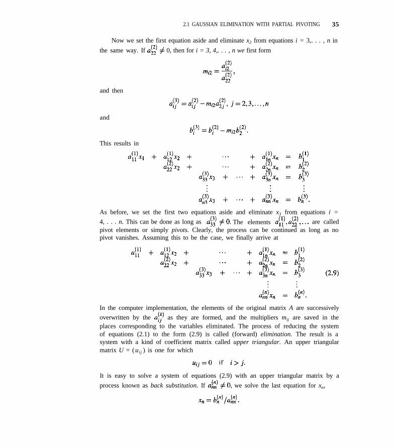
2.1 GAUSSIAN ELIMINATION WITH PARTIAL PIVOTING 35
Now we set the first equation aside and eliminate x2 from equations i = 3,. . . , n in
the same way. If 0, then for i = 3, 4,. . . , n we first form
and then
and
This results in
As before, we set the first two equations aside and eliminate x3 from equations i =
4, . . . n. This can be done as long as The elements are calledpivot elements or simply pivots. Clearly, the process can be continued as long as nopivot vanishes. Assuming this to be the case, we finally arrive at
In the computer implementation, the elements of the original matrix A are successively
overwritten by the as they are formed, and the multipliers mij are saved in theplaces corresponding to the variables eliminated. The process of reducing the systemof equations (2.1) to the form (2.9) is called (forward) elimination. The result is asystem with a kind of coefficient matrix called upper triangular. An upper triangularmatrix U = (u i j ) is one for which
It is easy to solve a system of equations (2.9) with an upper triangular matrix by a
process known as back substitution. If we solve the last equation for xn,
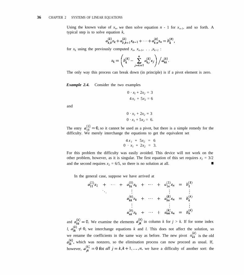
36 CHAPTER 2 SYSTEMS OF LINEAR EQUATIONS
Using the known value of xn, we then solve equation n - 1 for xn-1, and so forth. Atypical step is to solve equation k,
for xk using the previously computed xn, xn-1,. . . ,xk+1 :
The only way this process can break down (in principle) is if a pivot element is zero.
Example 2.4. Consider the two examples
0 · xl + 2x2 = 3
4 x1 + 5x2 = 6
and
0 · x1 + 2x2 = 3
0 · x1 + 5x2 = 6.
The entry so it cannot be used as a pivot, but there is a simple remedy for thedifficulty. We merely interchange the equations to get the equivalent set
4 x 1 + 5x2 = 60 · x1 + 2x2 = 3.
For this problem the difficulty was easily avoided. This device will not work on theother problem, however, as it is singular. The first equation of this set requires x2 = 3/2
and the second requires x2 = 6/5, so there is no solution at all. n
In the general case, suppose we have arrived at
and We examine the elements in column k for j > k. If for some index
l, we interchange equations k and l. This does not affect the solution, so
we rename the coefficients in the same way as before. The new pivot is the old
which was nonzero, so the elimination process can now proceed as usual. If,
however, we have a difficulty of another sort: the
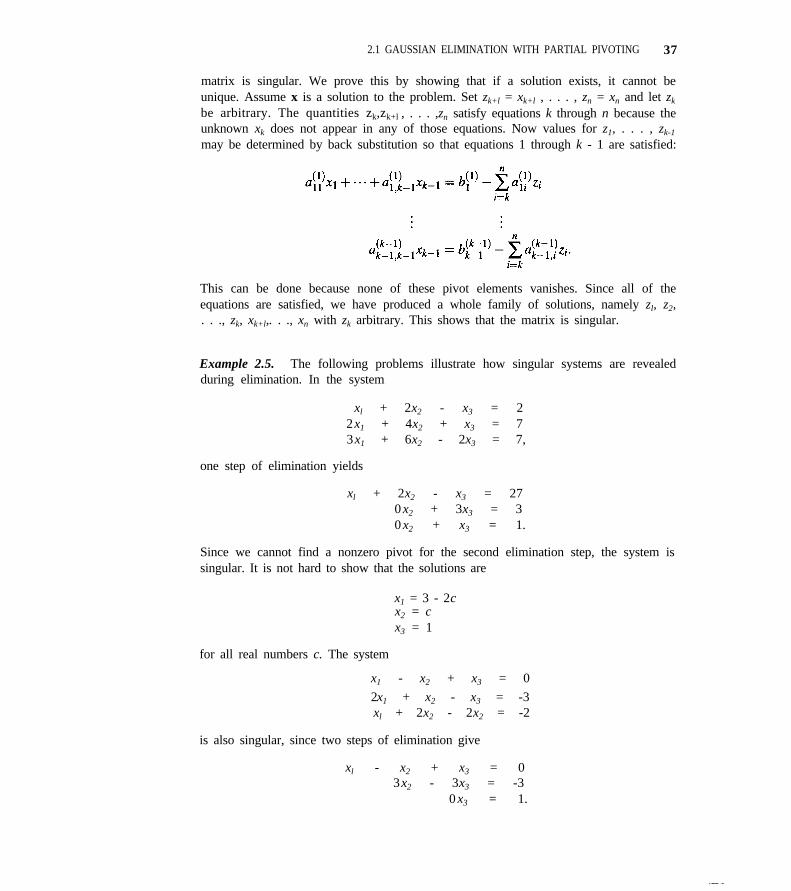
2.1 GAUSSIAN ELIMINATION WITH PARTIAL PIVOTING 37
matrix is singular. We prove this by showing that if a solution exists, it cannot beunique. Assume x is a solution to the problem. Set zk+l = xk+l , . . . , zn = xn and let zk
be arbitrary. The quantities zk,zk+l , . . . ,zn satisfy equations k through n because theunknown xk does not appear in any of those equations. Now values for z1, . . . , zk-1
may be determined by back substitution so that equations 1 through k - 1 are satisfied:
This can be done because none of these pivot elements vanishes. Since all of theequations are satisfied, we have produced a whole family of solutions, namely zl, z2,. . ., zk, xk+l,. . ., xn with zk arbitrary. This shows that the matrix is singular.
Example 2.5. The following problems illustrate how singular systems are revealedduring elimination. In the system
xl + 2x2 - x3 = 22x1 + 4x2 + x3 = 73x1 + 6x2 - 2x3 = 7,
one step of elimination yields
xl + 2x2 - x3 = 270 x2 + 3x3 = 30 x2 + x3 = 1.
Since we cannot find a nonzero pivot for the second elimination step, the system issingular. It is not hard to show that the solutions are
x1 = 3 - 2cx2 = cx3 = 1
for all real numbers c. The system
x1 - x2 + x3 = 0
2x1 + x2 - x3 = -3xl + 2x2 - 2x2 = -2
is also singular, since two steps of elimination give
xl - x2 + x3 = 03x2 - 3x3 = -3
0 x3 = 1.
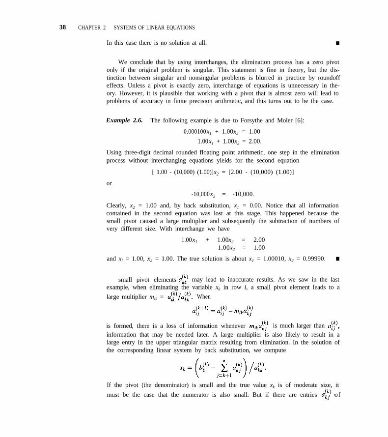
38 CHAPTER 2 SYSTEMS OF LINEAR EQUATIONS
In this case there is no solution at all. n
We conclude that by using interchanges, the elimination process has a zero pivotonly if the original problem is singular. This statement is fine in theory, but the dis-tinction between singular and nonsingular problems is blurred in practice by roundoffeffects. Unless a pivot is exactly zero, interchange of equations is unnecessary in the-ory. However, it is plausible that working with a pivot that is almost zero will lead toproblems of accuracy in finite precision arithmetic, and this turns out to be the case.
Example 2.6. The following example is due to Forsythe and Moler [6]:
0.000100x1 + 1.00x2 = 1.00
1.00x1 + 1.00x2 = 2.00.
Using three-digit decimal rounded floating point arithmetic, one step in the eliminationprocess without interchanging equations yields for the second equation
[ 1.00 - (10,000) (1.00)]x2 = [2.00 - (10,000) (1.00)]
or
-10,000x2 = -10,000.
Clearly, x2 = 1.00 and, by back substitution, x1 = 0.00. Notice that all informationcontained in the second equation was lost at this stage. This happened because thesmall pivot caused a large multiplier and subsequently the subtraction of numbers ofvery different size. With interchange we have
1.00x1 + 1.00x2 = 2.001.00x2 = 1.00
and xl = 1.00, x2 = 1.00. The true solution is about x1 = 1.00010, x2 = 0.99990. n
small pivot elements may lead to inaccurate results. As we saw in the lastexample, when eliminating the variable xk in row i, a small pivot element leads to a
large multiplier mik = When
is formed, there is a loss of information whenever is much larger thaninformation that may be needed later. A large multiplier is also likely to result in alarge entry in the upper triangular matrix resulting from elimination. In the solution ofthe corresponding linear system by back substitution, we compute
If the pivot (the denominator) is small and the true value xk is of moderate size, it
must be the case that the numerator is also small. But if there are entries of
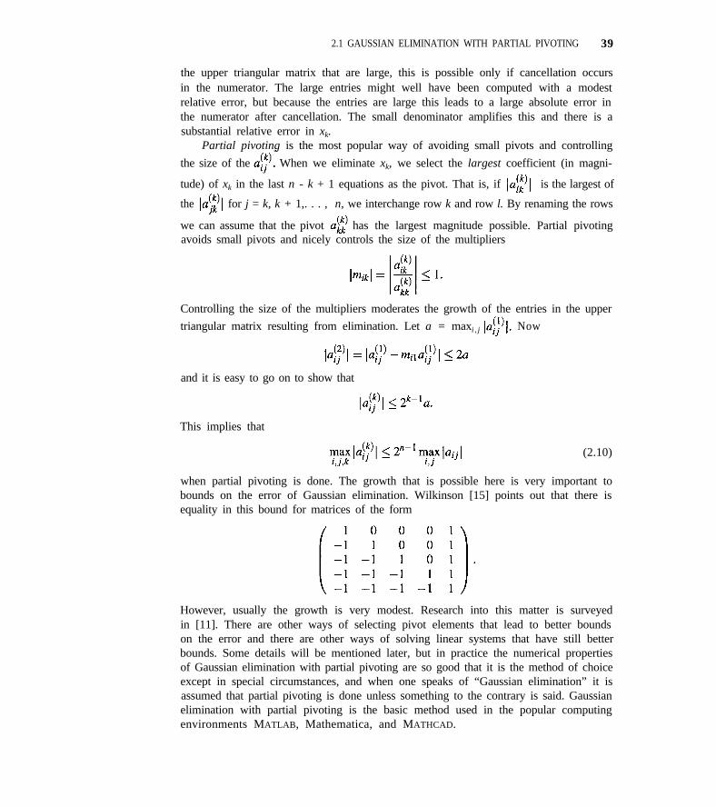
2.1 GAUSSIAN ELIMINATION WITH PARTIAL PIVOTING 39
the upper triangular matrix that are large, this is possible only if cancellation occursin the numerator. The large entries might well have been computed with a modestrelative error, but because the entries are large this leads to a large absolute error inthe numerator after cancellation. The small denominator amplifies this and there is asubstantial relative error in xk.
Partial pivoting is the most popular way of avoiding small pivots and controlling
the size of the When we eliminate xk, we select the largest coefficient (in magni-
tude) of xk in the last n - k + 1 equations as the pivot. That is, if is the largest of
the for j = k, k + 1,. . . , n, we interchange row k and row l. By renaming the rows
we can assume that the pivot has the largest magnitude possible. Partial pivotingavoids small pivots and nicely controls the size of the multipliers
Controlling the size of the multipliers moderates the growth of the entries in the upper
triangular matrix resulting from elimination. Let a = maxi , j Now
and it is easy to go on to show that
This implies that
(2.10)
when partial pivoting is done. The growth that is possible here is very important tobounds on the error of Gaussian elimination. Wilkinson [15] points out that there isequality in this bound for matrices of the form
However, usually the growth is very modest. Research into this matter is surveyedin [11]. There are other ways of selecting pivot elements that lead to better boundson the error and there are other ways of solving linear systems that have still betterbounds. Some details will be mentioned later, but in practice the numerical propertiesof Gaussian elimination with partial pivoting are so good that it is the method of choiceexcept in special circumstances, and when one speaks of “Gaussian elimination” it isassumed that partial pivoting is done unless something to the contrary is said. Gaussianelimination with partial pivoting is the basic method used in the popular computingenvironments MATLAB, Mathematica, and MATHCAD.
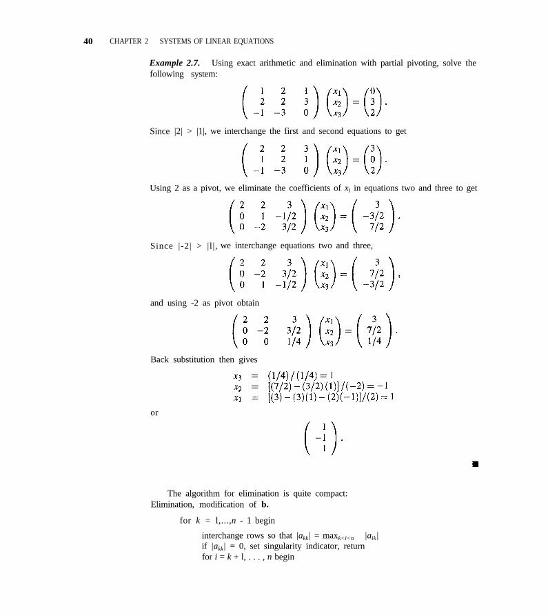
40 CHAPTER 2 SYSTEMS OF LINEAR EQUATIONS
Example 2.7. Using exact arithmetic and elimination with partial pivoting, solve thefollowing system:
Since |2| > |1|, we interchange the first and second equations to get
Using 2 as a pivot, we eliminate the coefficients of xl in equations two and three to get
Since |-2| > |l|, we interchange equations two and three,
and using -2 as pivot obtain
Back substitution then gives
or
The algorithm for elimination is quite compact:Elimination, modification of b.
for k = l,...,n - 1 begin
interchange rows so that |akk| = maxk<i<n |aik|if |akk| = 0, set singularity indicator, returnfor i = k + l, . . . , n begin
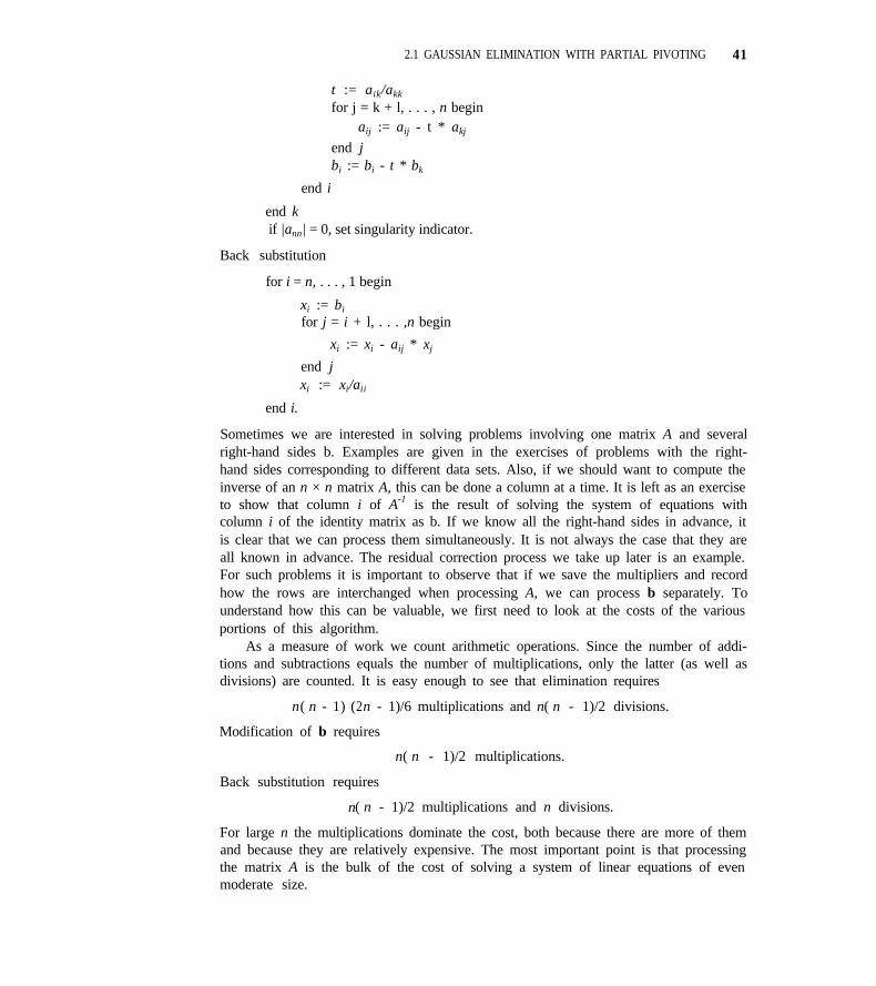
2.1 GAUSSIAN ELIMINATION WITH PARTIAL PIVOTING 41
t := aik/akk
for j = k + l, . . . , n beginaij := aij - t * akj
end jbi := bi - t * bk
end i
end kif |ann| = 0, set singularity indicator.
Back substitution
for i = n, . . . , 1 begin
xi := bi
for j = i + l, . . . ,n begin
xi := xi - aij * xj
end jxi := xi/aii
end i.
Sometimes we are interested in solving problems involving one matrix A and severalright-hand sides b. Examples are given in the exercises of problems with the right-hand sides corresponding to different data sets. Also, if we should want to compute theinverse of an n × n matrix A, this can be done a column at a time. It is left as an exerciseto show that column i of A-1 is the result of solving the system of equations withcolumn i of the identity matrix as b. If we know all the right-hand sides in advance, itis clear that we can process them simultaneously. It is not always the case that they areall known in advance. The residual correction process we take up later is an example.For such problems it is important to observe that if we save the multipliers and recordhow the rows are interchanged when processing A, we can process b separately. Tounderstand how this can be valuable, we first need to look at the costs of the variousportions of this algorithm.
As a measure of work we count arithmetic operations. Since the number of addi-tions and subtractions equals the number of multiplications, only the latter (as well asdivisions) are counted. It is easy enough to see that elimination requires
n( n - 1) (2n - 1)/6 multiplications and n( n - 1)/2 divisions.
Modification of b requires
n( n - 1)/2 multiplications.
Back substitution requires
n( n - 1)/2 multiplications and n divisions.
For large n the multiplications dominate the cost, both because there are more of themand because they are relatively expensive. The most important point is that processingthe matrix A is the bulk of the cost of solving a system of linear equations of evenmoderate size.
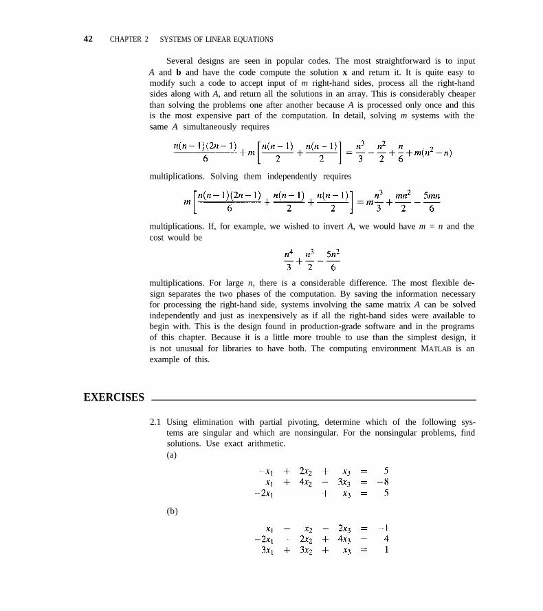
42 CHAPTER 2 SYSTEMS OF LINEAR EQUATIONS
Several designs are seen in popular codes. The most straightforward is to inputA and b and have the code compute the solution x and return it. It is quite easy tomodify such a code to accept input of m right-hand sides, process all the right-handsides along with A, and return all the solutions in an array. This is considerably cheaperthan solving the problems one after another because A is processed only once and thisis the most expensive part of the computation. In detail, solving m systems with thesame A simultaneously requires
multiplications. Solving them independently requires
multiplications. If, for example, we wished to invert A, we would have m = n and thecost would be
multiplications. For large n, there is a considerable difference. The most flexible de-sign separates the two phases of the computation. By saving the information necessaryfor processing the right-hand side, systems involving the same matrix A can be solvedindependently and just as inexpensively as if all the right-hand sides were available tobegin with. This is the design found in production-grade software and in the programsof this chapter. Because it is a little more trouble to use than the simplest design, itis not unusual for libraries to have both. The computing environment MATLAB is anexample of this.
EXERCISES
2.1 Using elimination with partial pivoting, determine which of the following sys-tems are singular and which are nonsingular. For the nonsingular problems, findsolutions. Use exact arithmetic.(a)
(b)
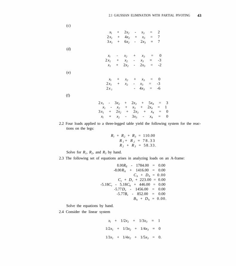
2.1 GAUSSIAN ELIMINATION WITH PARTIAL PIVOTING 43
(c)
xl + 2x2 - x3 = 22x1 + 4x2 + x3 = 73 x1 + 6x2 - 2x3 = 7
(d)
xl - x2 + x3 = 02 x1 + x2 - x3 = -3
x1 + 2x2 - 2x3 = -2
(e)
xl + x2 + x3 = 02x1 + x2 - x3 = -32 x 1 - 4x3 = -6
(f)
2 x1 - 3x2 + 2x3 + 5x4 = 3
3 x1 + 2x2 + 2x3 + x4 = 0x1 - x2 + x3 + 2x4 = 1
xl + x2 - 3x3 - x4 = 0
2.2 Four loads applied to a three-legged table yield the following system for the reac-tions on the legs:
Rl + R2 + R3 = 110.00R 1 + R 2 = 7 8 . 3 3R 2 + R 3 = 5 8 . 3 3 .
Solve for R1, R2, and R3 by hand.
2.3 The following set of equations arises in analyzing loads on an A-frame:
8.00RE - 1784.00 = 0.00-8.00RA + 1416.00 = 0.00
Ch + D h = 0.00Cv + Dv + 223.00 = 0.00
-5.18Cv - 5.18Ch + 446.00 = 0.00-5.77 Dv - 1456.00 = 0.00
-5.77Bv - 852.00 = 0.00Bh + D h = 0.00.
Solve the equations by hand.
2.4 Consider the linear system
xl + 1/2x2 + 1/3x3 = 1
1/2x1 + 1/3x2 + 1/4x3 = 0
1/3x1 + 1/4x2 + 1/5x3 = 0.
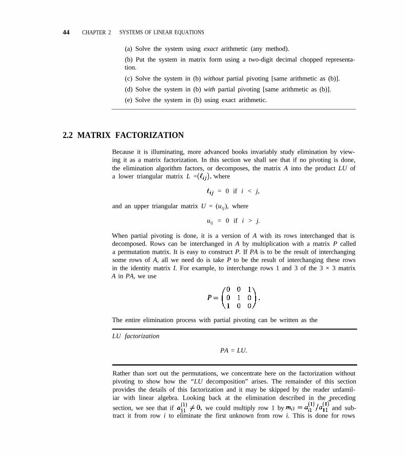
44 CHAPTER 2 SYSTEMS OF LINEAR EQUATIONS
(a) Solve the system using exact arithmetic (any method).
(b) Put the system in matrix form using a two-digit decimal chopped representa-tion.
(c) Solve the system in (b) without partial pivoting [same arithmetic as (b)].
(d) Solve the system in (b) with partial pivoting [same arithmetic as (b)].
(e) Solve the system in (b) using exact arithmetic.
2.2 MATRIX FACTORIZATION
Because it is illuminating, more advanced books invariably study elimination by view-ing it as a matrix factorization. In this section we shall see that if no pivoting is done,the elimination algorithm factors, or decomposes, the matrix A into the product LU ofa lower triangular matrix L = where
= 0 if i < j,
and an upper triangular matrix U = (uij), where
uij = 0 if i > j.
When partial pivoting is done, it is a version of A with its rows interchanged that isdecomposed. Rows can be interchanged in A by multiplication with a matrix P calleda permutation matrix. It is easy to construct P. If PA is to be the result of interchangingsome rows of A, all we need do is take P to be the result of interchanging these rowsin the identity matrix I. For example, to interchange rows 1 and 3 of the 3 × 3 matrixA in PA, we use
The entire elimination process with partial pivoting can be written as the
LU factorization
PA = LU.
Rather than sort out the permutations, we concentrate here on the factorization withoutpivoting to show how the “LU decomposition” arises. The remainder of this sectionprovides the details of this factorization and it may be skipped by the reader unfamil-iar with linear algebra. Looking back at the elimination described in the preceding
section, we see that if we could multiply row 1 by and sub-tract it from row i to eliminate the first unknown from row i. This is done for rows
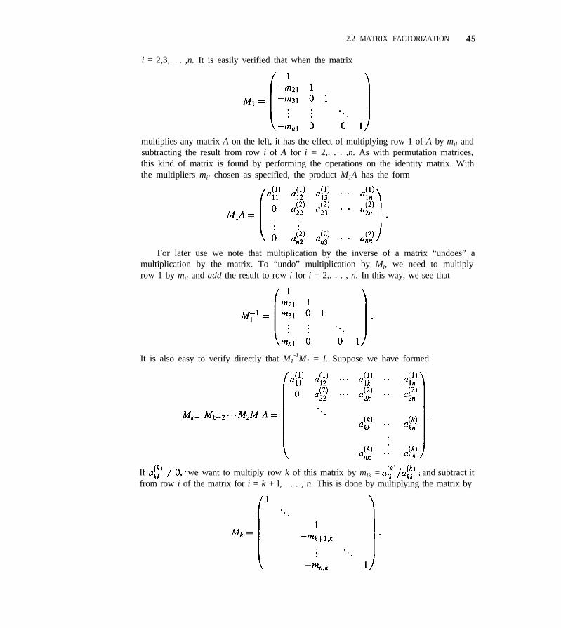
2.2 MATRIX FACTORIZATION 45
i = 2,3,. . . ,n. It is easily verified that when the matrix
multiplies any matrix A on the left, it has the effect of multiplying row 1 of A by mil andsubtracting the result from row i of A for i = 2,. . . ,n. As with permutation matrices,this kind of matrix is found by performing the operations on the identity matrix. Withthe multipliers mil chosen as specified, the product M1A has the form
For later use we note that multiplication by the inverse of a matrix “undoes” amultiplication by the matrix. To “undo” multiplication by Ml, we need to multiplyrow 1 by mil and add the result to row i for i = 2,. . . , n. In this way, we see that
It is also easy to verify directly that M1-1M1 = I. Suppose we have formed
If we want to multiply row k of this matrix by mik = and subtract itfrom row i of the matrix for i = k + l, . . . , n. This is done by multiplying the matrix by
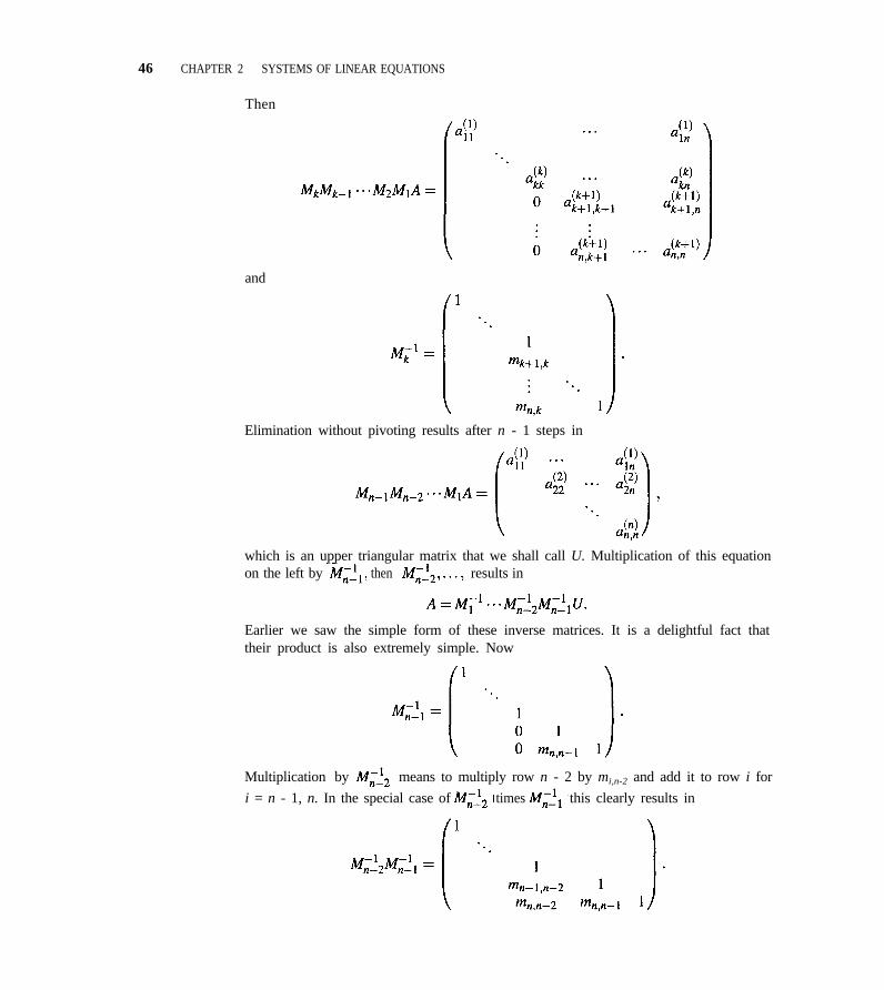
46 CHAPTER 2 SYSTEMS OF LINEAR EQUATIONS
Then
and
Elimination without pivoting results after n - 1 steps in
which is an upper triangular matrix that we shall call U. Multiplication of this equationon the left by then results in
Earlier we saw the simple form of these inverse matrices. It is a delightful fact thattheir product is also extremely simple. Now
Multiplication by means to multiply row n - 2 by mi,n-2 and add it to row i for
i = n - 1, n. In the special case of times this clearly results in
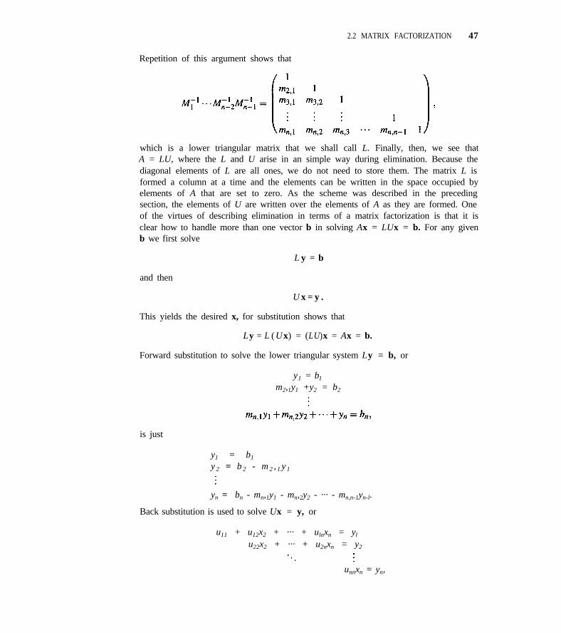
2.2 MATRIX FACTORIZATION 47
Repetition of this argument shows that
which is a lower triangular matrix that we shall call L. Finally, then, we see thatA = LU, where the L and U arise in an simple way during elimination. Because thediagonal elements of L are all ones, we do not need to store them. The matrix L isformed a column at a time and the elements can be written in the space occupied byelements of A that are set to zero. As the scheme was described in the precedingsection, the elements of U are written over the elements of A as they are formed. Oneof the virtues of describing elimination in terms of a matrix factorization is that it isclear how to handle more than one vector b in solving Ax = LUx = b. For any givenb we first solve
L y = b
and then
U x = y .
This yields the desired x, for substitution shows that
Ly = L ( Ux) = (LU)x = Ax = b.
Forward substitution to solve the lower triangular system Ly = b, or
y1 = b1
m2,1y1 +y2 = b2
is just
y1 = b1
y 2 = b 2 - m 2 , 1 y 1
yn = bn - mn,1y1 - mn,2y2 - ··· - mn,n-1yn-l.
Back substitution is used to solve Ux = y, or
u11 + u12x2 + ··· + ulnxn = yl
u22x2 + ··· + u2nxn = y2
unnxn = yn,
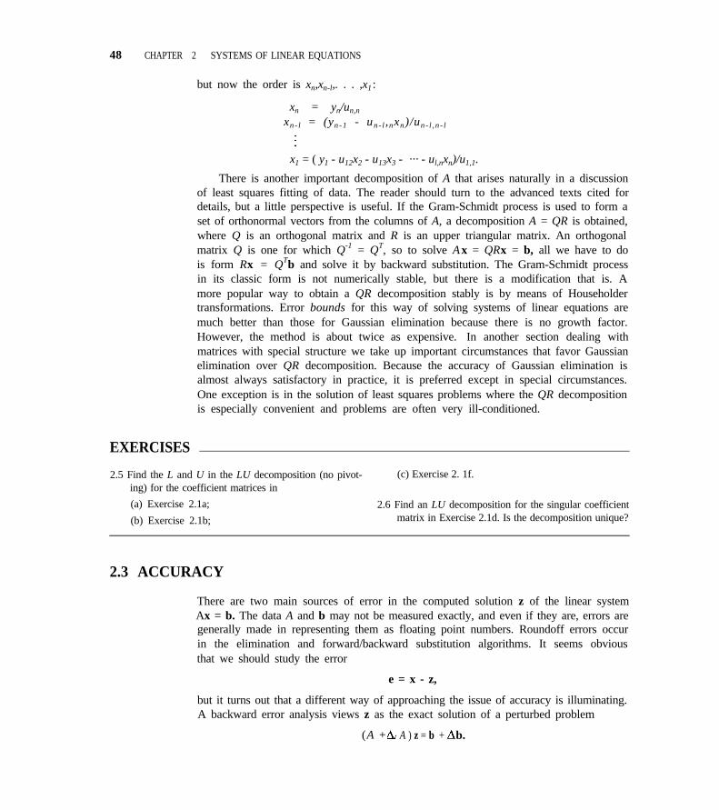
48 CHAPTER 2 SYSTEMS OF LINEAR EQUATIONS
but now the order is xn,xn-l,. . . ,x1 :
xn = yn/un,n
xn- l = (yn-1 - un- l ,nxn)/un- l , n - l
x1 = ( y1 - u12x2 - u13x3 - ··· - ul,nxn)/u1,1.
There is another important decomposition of A that arises naturally in a discussionof least squares fitting of data. The reader should turn to the advanced texts cited fordetails, but a little perspective is useful. If the Gram-Schmidt process is used to form aset of orthonormal vectors from the columns of A, a decomposition A = QR is obtained,where Q is an orthogonal matrix and R is an upper triangular matrix. An orthogonalmatrix Q is one for which Q-1 = QT, so to solve Ax = QRx = b, all we have to dois form Rx = QTb and solve it by backward substitution. The Gram-Schmidt processin its classic form is not numerically stable, but there is a modification that is. Amore popular way to obtain a QR decomposition stably is by means of Householdertransformations. Error bounds for this way of solving systems of linear equations aremuch better than those for Gaussian elimination because there is no growth factor.However, the method is about twice as expensive. In another section dealing withmatrices with special structure we take up important circumstances that favor Gaussianelimination over QR decomposition. Because the accuracy of Gaussian elimination isalmost always satisfactory in practice, it is preferred except in special circumstances.One exception is in the solution of least squares problems where the QR decompositionis especially convenient and problems are often very ill-conditioned.
EXERCISES
2.5 Find the L and U in the LU decomposition (no pivot- (c) Exercise 2. 1f.ing) for the coefficient matrices in
(a) Exercise 2.1a; 2.6 Find an LU decomposition for the singular coefficient
(b) Exercise 2.1b; matrix in Exercise 2.1d. Is the decomposition unique?
2.3 ACCURACY
There are two main sources of error in the computed solution z of the linear systemAx = b. The data A and b may not be measured exactly, and even if they are, errors aregenerally made in representing them as floating point numbers. Roundoff errors occurin the elimination and forward/backward substitution algorithms. It seems obviousthat we should study the error
e = x - z,
but it turns out that a different way of approaching the issue of accuracy is illuminating.A backward error analysis views z as the exact solution of a perturbed problem
(A + A ) z = b + b.
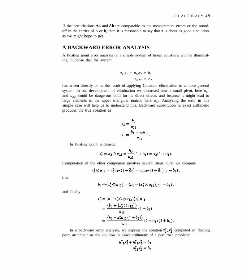
2.3 ACCURACY 49
If the perturbations, and are comparable to the measurement errors or the round-off in the entries of A or b, then it is reasonable to say that z is about as good a solutionas we might hope to get.
A BACKWARD ERROR ANALYSISA floating point error analysis of a simple system of linear equations will be illuminat-ing. Suppose that the system
u11x1 + u12x2 = b1
u22x2 = b2
has arisen directly or as the result of applying Gaussian elimination to a more generalsystem. In our development of elimination we discussed how a small pivot, here u11
and u22, could be dangerous both for its direct effects and because it might lead tolarge elements in the upper triangular matrix, here u12. Analyzing the error in thissimple case will help us to understand this. Backward substitution in exact arithmeticproduces the true solution as
In floating point arithmetic,
Computation of the other component involves several steps. First we compute
then
and finally
In a backward error analysis, we express the solution computed in floatingpoint arithmetic as the solution in exact arithmetic of a perturbed problem:

50 CHAPTER 2 SYSTEMS OF LINEAR EQUATIONS
As the notation suggests, this can be done without perturbing the right-hand side ofthe equation. The equation
will be valid if we define
Similarly, the equation
will be valid if we define
With these definitions we have expressed the computed solution of the given prob-lem as the exact solution of a problem with perturbed matrix. It is seen that none ofthe coefficients of the matrix is perturbed by more than about two units of roundoff.
This analysis tells us that the backward substitution algorithm is sure to produce agood result in the sense that the computed solution is the exact solution of a problemclose to the one given. However, that is not the same as saying that the computedsolution is close to the true solution. A forward error analysis bounds directly thedifference between the computed and true solutions.
Our basic assumption about floating point arithmetic is that a single operation iscarried out with a relative error bounded by the unit of roundoff u, so we have
Substitution of the expressions developed earlier and a little manipulation shows that
where
This implies that
2.3 ACCURACY 51
According to this bound, the relative error is generally small. A large relative erroris possible only when |x2u12| >> |x1u11|. If the solution is such that both componentsare of comparable size, a large relative error is possible only when the pivot u11 issmall and/or the entry u12 in the upper triangular matrix is large. Large relative errorsare more likely when |x2| >> |x1|. The denominator can be written in the form
xlu11 = b1 - x2u12,
showing that the relative error can be large when the numerator is large and the de-nominator is small because of cancellation.
ROUNDOFF ANALYSISA natural way to measure the quality of an approximate solution z is by how well itsatisfies the equation. A virtue of this is that it is easy to compute the residual
r = b - Az .
In this measure, a good solution z has a small residual. Because of cancellation (seeExample 1.10), if we should want an accurate residual for a good solution, it will benecessary to compute it in higher precision arithmetic, and this may not be available.The residual provides a for the backward error analysis, namely,
= -r.
The residual r is connected to the error e by
r = b - Az = Ax - Az = A(x - z) = Ae
or e = A-1 r. A small residual r, hence a small may be perfectly satisfactory fromthe point of view of backward error analysis even when the corresponding error e isnot small.
Example 2.8. To illustrate the distinction between the two points of view, considerthe system
(2.11)
We carry out the elimination process using three-digit chopped decimal arithmetic.After the first step we have
It then follows that
z1 = (0.200 - 0.547z 2)/0.747 = 0.267,
52 CHAPTER 2 SYSTEMS OF LINEAR EQUATIONS
so the computed solution is
The exact solution to (2.11) is easily found to be xl = 1 and x2 = -1. Therefore theerror (in exact arithmetic) is
In contrast, the residual (in exact arithmetic) is
r = b - Az
This says that z is the exact solution of Az = b + where b1 = 0.200 is perturbed to0.199449 and b2 is perturbed to 0.166341. Thus, z is the solution of a problem veryclose to the one posed, even though it differs considerably from the solution x of theoriginal problem. n
The fundamental difficulty in Example 2.8 is that the matrix in the system (2.11)is nearly singular. In fact, the first equation is, to within roundoff error, 1.2 times thesecond. If we examine the elimination process we see that z2 was computed from twoquantities that were themselves on the order of roundoff error. Carrying more digits inour arithmetic would have produced a totally different z2. The error in z2 propagatesto an error in z1. This accounts for the computed solution being in error. Why thenare the residuals small? Regardless of z2, the number z1 was computed to make theresidual for the first equation as nearly zero as possible in the arithmetic being used.The residual for the second equation should also be small because the system is closeto singular: the first equation is approximately a multiple of the second. In Section 2.2we observed that any matrix A could have its rows interchanged to obtain a matrixPA, which can be decomposed as the product of a lower triangular matrix L and anupper triangular matrix U. For simplicity we ignore the permutation matrix P in whatfollows. An error analysis of elimination using floating point arithmetic shows that Land U are computed with errors and respectively. Then A is not exactly equalto the product (L + ) (U + ). Let be defined so that
that is,
2.3 ACCURACY 53
We might reasonably hope to compute L with errors M that are small relative to L, andthe same for U. However, the expression for AA shows that the sizes of L and U playimportant roles in how well A is represented by the computed factors. Partial pivotingkeeps the elements of L less than or equal to 1 in magnitude. We also saw in (2.10) that
the size of elements of U, the was moderated with partial pivoting. In particular,
they cannot exceed 2n-1 maxij |aij| for an n × n matrix. It can be shown rigorously, ontaking into account the errors of decomposition and of forward/backward substitution,that the computed solution z of Ax = b satisfies
(A + )z = b, (2.12)
where the entries of are usually small. To make precise how small these entriesare, we need a way of measuring the sizes of vectors and matrices. One way to mea-sure the size of a vector x of n components is by its norm, which is denoted by ||x||.Several definitions of norm are common in numerical analysis. One that is likely to be
familiar is the Euclidean length of x, All vector norms possess many ofthe properties of length. The norm used in this chapter is the maximum norm
(2.13)
If A is an n × n matrix and x is an n -vector, then Ax is also an n-vector. A matrix normcan be defined in terms of a vector norm by
(2.14)
Geometrically, this says that ||A|| is the maximum relative distortion that the matrix Acreates when it multiplies a vector x 0. It is not easy to evaluate ||A|| directly from(2.14), but it can be shown that for the maximum norm (2.13)
(2.15)
which is easy enough to evaluate. An important inequality connects norms of vectorsand matrices:
||Ax|| < ||A|| ||x||. (2.16)
For x 0 this follows immediately from the definition (2.14). For x = 0 we note thatA x = 0 and that ||x|| = 0, from which the inequality is seen to hold.
Example 2.9. Let x =
||x|| = max [| - 1|, |2|, |3|] = 3.

54 CHAPTER 2 SYSTEMS OF LINEAR EQUATIONS
Let A =
||A|| = [(|l| + |-l| + |0|), (|2|+ |-2| + |3|), (|-4| + |1| + |-1|)]= max[(2), (7), (6)] = 7.
Returning to the roundoff analysis for Gaussian elimination, it can be shown rig-orously [11] that the computed solution z satisfies the perturbed equation (2.12) where
(2.17)
As usual, u is the unit roundoff. The factor γn depends on n and can grow as fastas 2n-1. To put this in perspective, suppose that AA arises from rounding A to formmachine numbers. Then could be as large as u|aij| and could be as largeas
According to the bounds, the perturbations due to the decomposition and forward/back-ward substitution process are at worst a factor of γn times the error made in the initialrounding of the entries of A. If the rigorous bound 2n-1 on γn truly reflected prac-tice, we would have to resort to another algorithm for large n. Fortunately, for mostproblems γn is more like 10, independent of the size of n.
From this it can be concluded that Gaussian elimination practically always pro-duces a solution z that is the exact solution of a problem close to the one posed. SinceAz - b = the residual r satisfies
This says that the size of the residual is nearly always small relative to the sizes of Aand z. However, recall that this does not imply that the actual error e is small.
For additional insight as to why Gaussian elimination tends to produce solutionswith small residuals, think of the LU factorization of A discussed in Section 2.2. Theforward substitution process used to solve the lower triangular system Ly = b succes-sively computes y1, y2,. . . , yn so as to make the residual zero. For example, regardlessof the errors in y1 and m2,1 the value of y2 is computed so that
m2,lyl + y2 = b2,
that is, the residual of this equation is zero (in exact arithmetic) with this value of y2.The same thing happens in the back substitution process to compute xn,xn-1,. . . ,x1
that satisfy Ux = y. Thus, the very nature of the process responds to errors in thedata in such a way as to yield a small residual. This is not at all true when x iscomputed by first calculating the inverse A-1 and then forming A-l b. With a littleextra work it is possible to make Gaussian elimination stable in a very strong sense.
2.3 ACCURACY 55
Suppose that we have solved Ax = b to obtain an approximate solution z. We canexpect it to have some accuracy, although perhaps not all the accuracy possible in theprecision used. A little manipulation shows that the error e = x - z satisfies A e = r,where r is the residual of the approximate solution z. We have seen that if Gaussianelimination is organized properly, it is inexpensive to solve this additional system ofequations. Of course, we do not expect to solve it exactly either, but we do expectthat the computed approximation d to the error in z will have some accuracy. If itdoes, w = z + d will approximate x better than z does. In principle this process, callediterative refinement, can be repeated to obtain an approximation to x correct in all itsdigits. The trouble in practice is that for the process to work as described, we have tohave an accurate residual, and the better the approximate solution, the more difficultthis is to obtain. Skeel [14] has shown that just one step of iterative refinement withthe residual computed in the working precision will provide a computed solution thatis very satisfactory. This solution will have a small residual and will satisfy exactlya system of equations with each coefficient differing slightly from that of the givensystem. This is much better than the result for z that states that the perturbation ina coefficient is small compared to the norm of the whole matrix, not that it is smallcompared to the coefficient itself. So, if we are concerned about the reliability ofGaussian elimination with partial pivoting, we could save copies of the matrix andright-hand side and perform one step of iterative refinement in the working precisionto correct the result as necessary.
NORM BOUNDS FOR THE ERROR
In the preceding subsection, we found that roundoff errors in the algorithm could beconsidered equivalent to errors in the data A. We now study the effect of such pertur-bations, as well as errors in the given data, on the error e. For simplicity, let us firstconsider the case where only the data b is in error. Let x + be the solution of
Multiply this by A-1 and use the fact that x = A-lb to get
(2.18)
Norm inequalities say that
But b = Ax similarly implies ||b|| < ||A|| ||x||, hence
(2.19)
(2.20)
Inequality (2.19) says that in an absolute sense, input errors can be amplified byas much as ||A-1|| in the solution. In contrast, (2.20) says that in a relative sense, inputerrors can be magnified by as much as ||A|| ||A-1||. The important quantity ||A|| ||A-1||denoted by cond(A) is called the
56 CHAPTER 2 SYSTEMS OF LINEAR EQUATIONS
condition number of A
cond(A) = ||A|| ||A-l||.
A theorem that helps us understand the condition number is
In words this says that there is a singular matrix S that differs from A in a relativesense by the reciprocal of the condition number of A. Put differently, if A has a “large”condition number, it is “close” to a singular matrix.
The condition number clearly depends on the norm, but in this book we consideronly the maximum norm (2. 15).
Example 2.10. For A , find ||A||,||A-l||, cond(A ). First,
||A|| = max[(|l|+|2|),(|3|+|4|)] = max[(3),(7)] = 7.
For 2 x 2 matrices, the inverse matrix is easy to work out. If A =
So, in our case
and
Then
Example 2.11. The matrix
is much closer to being singular than the matrix in Example 2.10 since
(2.21)
2.3 ACCURACY 57
and
||A|| = 2, ||A-l|| = 2 x 10⁵, cond(A) = 4 x 10⁵.
The theorem about the condition number says that there is asingular matrix that iswithin 1/cond(A) = 2.5 x 10⁻⁶ of A. Although not quite this close, the simple matrix
is obviously singular and
The effect of perturbing A is more complicated because it is possible that A + ∆ A issingular. However, if the perturbation is sufficiently small, say ||A–1|| ||∆ A|| < 1, thenit can be shown [9] that A + ∆ A is nonsingular and further that if (A + ∆A) (x + ∆x) =b + ∆b, then we have the so-called
condition number inequality
valid for ||A–l|| ||∆ A|| < 1.
(2.22)
Inequality (2. 17) and the related discussion say that rounding errors in the course ofGaussian elimination are equivalent to solving a perturbed system for which we usu-ally have
(2.23)
where u is the unit roundoff. In some applications data errors maybe much larger thanthis, and they must be used in (2.22).
Example 2.12. Suppose we solve Ax = b on a machine with u = 5 x 10–11 andobtain
Then from (2.22), assuming exact data so that ||∆A||/||A|| 5 x 10⁻¹⁰, the bound onthe relative error is
58 CHAPTER 2 SYSTEMS OF LINEAR EQUATIONS
On the other hand, if the data are known to be in error, say andthen
With ||x|| ||z|| 18.6 the absolute error bound is 0.37, so this analysis says that
xl = 6.23 ± 0.37
x2 = 18.62 ± 0.37.
One criticism of the analysis based on norms is that it is a worst-case analysis.The condition number does not depend on b, so the inequality (2.22) must allow forthe worst choice of b and A large condition number is cause for concern, but itdoes not mean a given problem will be solved inaccurately. Furthermore, the fact that
is small does not mean that for each i, is small.
OTHER ERROR EXPRESSIONS AND APPROXIMATIONSA better understanding of the size of the error can be obtained with a more carefulanalysis. Again, it is simpler to consider first only changes in b. If the entries of A-1
are denoted by then in component form is
(2.24)
Hence, for
is the exact formula for the relative change in xi as a function of the relative changesin the bp. The special case of a change in only one entry of b is
(2.25)
and
(2.26)
This says that the relative error of a solution component xi will be sensitive to therelative error in a data component bp whenever the factor is large. The resultsusing norms told us that “large” components in the inverse matrix indicate possiblesensitivity to errors in the data. This result goes much further. It brings to our attentionthat “small” components in the solution vector indicate possible sensitivity to errors inthe data. More to the point, it shows which components are sensitive and how much.
2.3 ACCURACY 59
What if A is perturbed? For simplicity we study the effect on a solution componentxi when only a single entry apq of A is altered. In component form Ax = b is
Taking the partial derivative with respect to apq leads to
and
In terms of the vectors
w = (w i), where wi = 0 for i p, wp= -xq,
this is a system of equations Av = w. Then v = A-1w, or in component form,
We conclude that for “small” perturbations of apq, the solution component xi isperturbed to xi + where
In terms of relative changes, this is
(2.27)
This approximate result shows much more detail than the bound (2.22). In particular,it is clear that if there is a solution component xq that is large compared to a componentxi, then xi can be sensitive to perturbations in column q of A.
ESTIMATING CONDITIONAlthough there is far more information in the equality (2.26) and the approxima-tion (2.27) than in the condition number inequality (2.22), they require knowledgeof A-1, which is relatively expensive to compute. An efficient algorithm for the cal-culation of A-1 requires roughly three times the work needed for elimination. Tocompute cond(A) exactly requires A-l, but for our purposes an estimate for ||A-1||
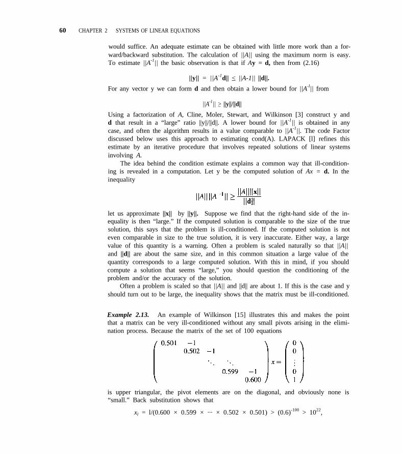
60 CHAPTER 2 SYSTEMS OF LINEAR EQUATIONS
would suffice. An adequate estimate can be obtained with little more work than a for-ward/backward substitution. The calculation of ||A|| using the maximum norm is easy.To estimate ||A-1|| the basic observation is that if Ay = d, then from (2.16)
||y|| = ||A-1d|| < ||A-1|| ||d||.
For any vector y we can form d and then obtain a lower bound for ||A-l|| from
||A-1|| > ||y||/||d||
Using a factorization of A, Cline, Moler, Stewart, and Wilkinson [3] construct y andd that result in a “large” ratio ||y||/||d||. A lower bound for ||A-1|| is obtained in anycase, and often the algorithm results in a value comparable to ||A-1||. The code Factordiscussed below uses this approach to estimating cond(A). LAPACK [l] refines thisestimate by an iterative procedure that involves repeated solutions of linear systemsinvolving A.
The idea behind the condition estimate explains a common way that ill-condition-ing is revealed in a computation. Let y be the computed solution of Ax = d. In theinequality
let us approximate ||x|| by ||y||. Suppose we find that the right-hand side of the in-equality is then “large.” If the computed solution is comparable to the size of the truesolution, this says that the problem is ill-conditioned. If the computed solution is noteven comparable in size to the true solution, it is very inaccurate. Either way, a largevalue of this quantity is a warning. Often a problem is scaled naturally so that ||A||and ||d|| are about the same size, and in this common situation a large value of thequantity corresponds to a large computed solution. With this in mind, if you shouldcompute a solution that seems “large,” you should question the conditioning of theproblem and/or the accuracy of the solution.
Often a problem is scaled so that ||A|| and ||d|| are about 1. If this is the case and yshould turn out to be large, the inequality shows that the matrix must be ill-conditioned.
Example 2.13. An example of Wilkinson [15] illustrates this and makes the pointthat a matrix can be very ill-conditioned without any small pivots arising in the elimi-nation process. Because the matrix of the set of 100 equations
is upper triangular, the pivot elements are on the diagonal, and obviously none is“small.” Back substitution shows that
xl = l/(0.600 × 0.599 × ··· × 0.502 × 0.501) > (0.6)-100 > 1022,
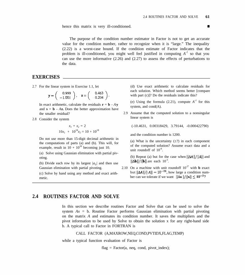
2.4 ROUTINES FACTOR AND SOLVE 61
hence this matrix is very ill-conditioned. n
The purpose of the condition number estimator in Factor is not to get an accuratevalue for the condition number, rather to recognize when it is “large.” The inequality(2.22) is a worst-case bound. If the condition estimate of Factor indicates that theproblem is ill-conditioned, you might well feel justified in computing A-1 so that youcan use the more informative (2.26) and (2.27) to assess the effects of perturbations tothe data.
EXERCISES
2.7
2.8
For the linear system in Exercise 1.1, let
In exact arithmetic, calculate the residuals r = b - Ayand s = b - Az. Does the better approximation havethe smaller residual? 2.9
Consider the system
x1 + x2 = 2
10x1 + 1018x2 = 10 + 1018
Do not use more than 15-digit decimal arithmetic inthe computations of parts (a) and (b). This will, forexample, result in 10 + 1018 becoming just 10.
(a) Solve using Gaussian elimination with partial piv-oting.
(b) Divide each row by its largest |aij| and then useGaussian elimination with partial pivoting. 2.10
(c) Solve by hand using any method and exact arith-metic.
(d) Use exact arithmetic to calculate residuals foreach solution. Which method seems better [comparewith part (c)]? Do the residuals indicate this?
(e) Using the formula (2.21), compute A-1 for thissystem, and cond(A).
Assume that the computed solution to a nonsingularlinear system is
(-10.4631, 0.00318429, 3.79144, -0.000422790)
and the condition number is 1200.
(a) What is the uncertainty (±?) in each componentof the computed solution? Assume exact data and aunit roundoff of 10-6.
(b) Repeat (a) but for the case when andare each 10-5.
On a machine with unit roundoff 10-l7 with b exactbut how large a condition num-ber can we tolerate if we want
2.4 ROUTINES FACTOR AND SOLVE
In this section we describe routines Factor and Solve that can be used to solve thesystem Ax = b. Routine Factor performs Gaussian elimination with partial pivotingon the matrix A and estimates its condition number. It saves the multipliers and thepivot information to be used by Solve to obtain the solution x for any right-hand sideb. A typical call to Factor in FORTRAN is
CALL FACTOR (A,MAXROW,NEQ,COND,PVTIDX,FLAG,TEMP)
while a typical function evaluation of Factor is
flag = Factor(a, neq, cond, pivot_index);
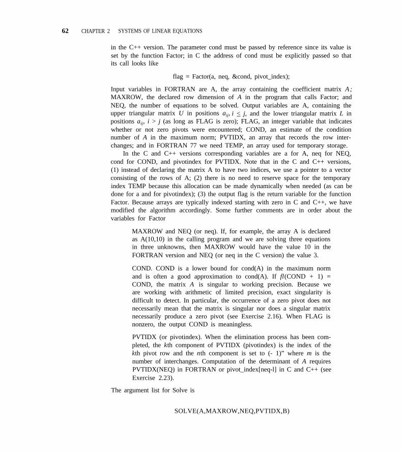
62 CHAPTER 2 SYSTEMS OF LINEAR EQUATIONS
in the C++ version. The parameter cond must be passed by reference since its value isset by the function Factor; in C the address of cond must be explicitly passed so thatits call looks like
flag = Factor(a, neq, &cond, pivot_index);
Input variables in FORTRAN are A, the array containing the coefficient matrix A;MAXROW, the declared row dimension of A in the program that calls Factor; andNEQ, the number of equations to be solved. Output variables are A, containing theupper triangular matrix U in positions aij, i < j, and the lower triangular matrix L inpositions aij, i > j (as long as FLAG is zero); FLAG, an integer variable that indicateswhether or not zero pivots were encountered; COND, an estimate of the conditionnumber of A in the maximum norm; PVTIDX, an array that records the row inter-changes; and in FORTRAN 77 we need TEMP, an array used for temporary storage.
In the C and C++ versions corresponding variables are a for A, neq for NEQ,cond for COND, and pivotindex for PVTIDX. Note that in the C and C++ versions,(1) instead of declaring the matrix A to have two indices, we use a pointer to a vectorconsisting of the rows of A; (2) there is no need to reserve space for the temporaryindex TEMP because this allocation can be made dynamically when needed (as can bedone for a and for pivotindex); (3) the output flag is the return variable for the functionFactor. Because arrays are typically indexed starting with zero in C and C++, we havemodified the algorithm accordingly. Some further comments are in order about thevariables for Factor
MAXROW and NEQ (or neq). If, for example, the array A is declaredas A(10,10) in the calling program and we are solving three equationsin three unknowns, then MAXROW would have the value 10 in theFORTRAN version and NEQ (or neq in the C version) the value 3.
COND. COND is a lower bound for cond(A) in the maximum normand is often a good approximation to cond(A). If fl(COND + 1) =COND, the matrix A is singular to working precision. Because weare working with arithmetic of limited precision, exact singularity isdifficult to detect. In particular, the occurrence of a zero pivot does notnecessarily mean that the matrix is singular nor does a singular matrixnecessarily produce a zero pivot (see Exercise 2.16). When FLAG isnonzero, the output COND is meaningless.
PVTIDX (or pivotindex). When the elimination process has been com-pleted, the kth component of PVTIDX (pivotindex) is the index of thekth pivot row and the nth component is set to (- 1)” where m is thenumber of interchanges. Computation of the determinant of A requiresPVTIDX(NEQ) in FORTRAN or pivot_index[neq-l] in C and C++ (seeExercise 2.23).
The argument list for Solve is
SOLVE(A,MAXROW,NEQ,PVTIDX,B)
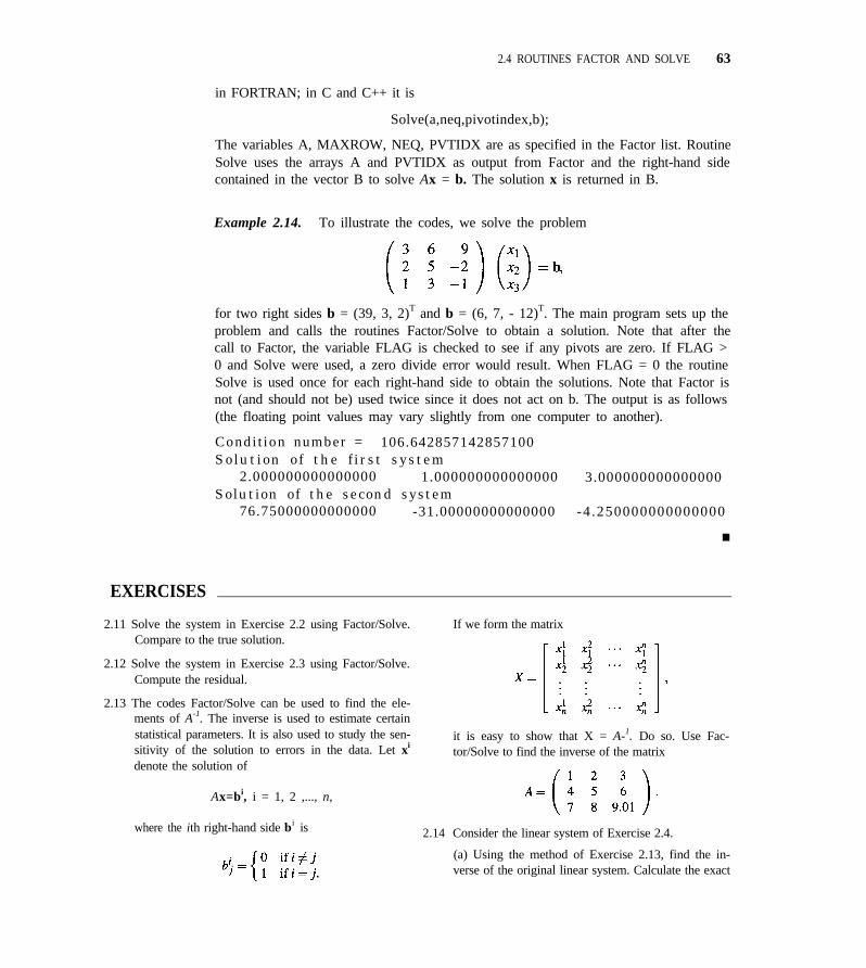
2.4 ROUTINES FACTOR AND SOLVE
in FORTRAN; in C and C++ it is
Solve(a,neq,pivotindex,b);
63
The variables A, MAXROW, NEQ, PVTIDX are as specified in the Factor list. RoutineSolve uses the arrays A and PVTIDX as output from Factor and the right-hand sidecontained in the vector B to solve Ax = b. The solution x is returned in B.
Example 2.14. To illustrate the codes, we solve the problem
for two right sides b = (39, 3, 2)T and b = (6, 7, - 12)T. The main program sets up theproblem and calls the routines Factor/Solve to obtain a solution. Note that after thecall to Factor, the variable FLAG is checked to see if any pivots are zero. If FLAG >0 and Solve were used, a zero divide error would result. When FLAG = 0 the routineSolve is used once for each right-hand side to obtain the solutions. Note that Factor isnot (and should not be) used twice since it does not act on b. The output is as follows(the floating point values may vary slightly from one computer to another).
Condi t ion number = 106.642857142857100Solution of the first system
2.000000000000000 1.000000000000000 3.000000000000000Solution of the second system
76.75000000000000 -31.00000000000000 -4 .250000000000000
n
EXERCISES
2.11 Solve the system in Exercise 2.2 using Factor/Solve.Compare to the true solution.
2.12 Solve the system in Exercise 2.3 using Factor/Solve.Compute the residual.
2.13 The codes Factor/Solve can be used to find the ele-ments of A-1. The inverse is used to estimate certainstatistical parameters. It is also used to study the sen-sitivity of the solution to errors in the data. Let xi
denote the solution of
Ax=bi, i = 1, 2 ,..., n,
where the ith right-hand side bi is
If we form the matrix
it is easy to show that X = A-1. Do so. Use Fac-tor/Solve to find the inverse of the matrix
2.14 Consider the linear system of Exercise 2.4.
(a) Using the method of Exercise 2.13, find the in-verse of the original linear system. Calculate the exact
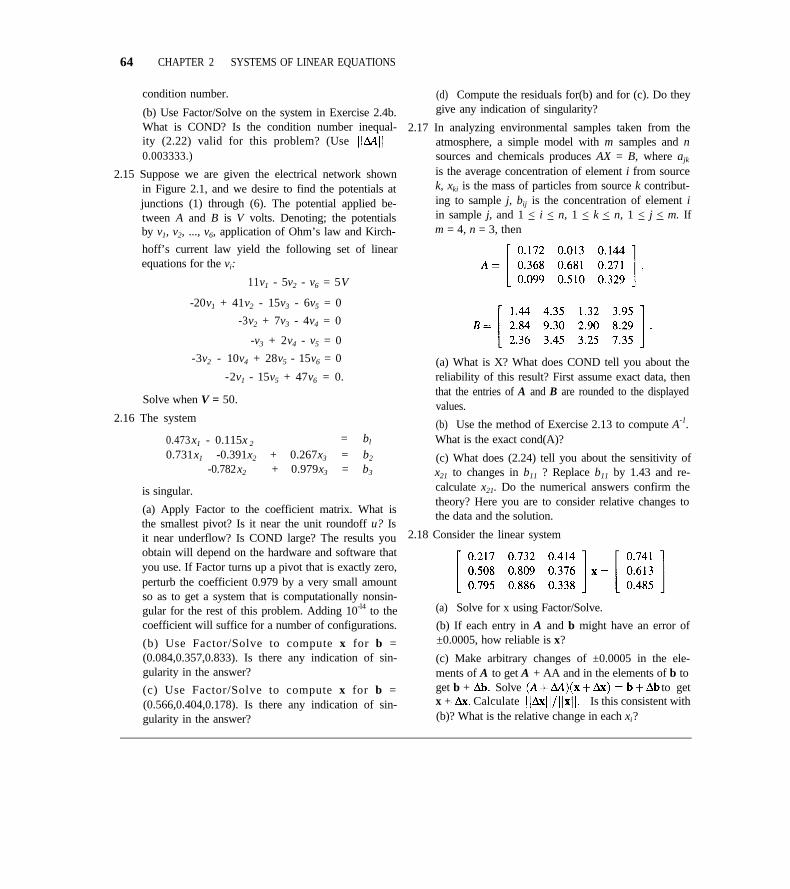
64 CHAPTER 2 SYSTEMS OF LINEAR EQUATIONS
condition number.
(b) Use Factor/Solve on the system in Exercise 2.4b.What is COND? Is the condition number inequal-ity (2.22) valid for this problem? (Use0.003333.)
2.15 Suppose we are given the electrical network shownin Figure 2.1, and we desire to find the potentials atjunctions (1) through (6). The potential applied be-tween A and B is V volts. Denoting; the potentials
(d) Compute the residuals for(b) and for (c). Do theygive any indication of singularity?
2.17 In analyzing environmental samples taken from theatmosphere, a simple model with m samples and nsources and chemicals produces AX = B, where ajk
is the average concentration of element i from sourcek, xki is the mass of particles from source k contribut-ing to sample j, bij is the concentration of element iin sample j, and 1 < i < n, 1 < k < n, 1 < j < m. If
by v1, v2, ..., v6, application of Ohm’s law and Kirch-
hoff’s current law yield the following set of linearequations for the vi:
11v1 - 5v2 - v6 = 5V
m = 4, n = 3, then
-20v1 + 41v2 - 15v3 - 6v5 = 0
-3v2 + 7v3 - 4v4 = 0
-v3 + 2v4 - v5 = 0
-3v2 - 10v4 + 28v5 - 15v6 = 0
-2v1 - 15v5 + 47v6 = 0.
Solve when V = 50.
2.16 The system
0.473x1 - 0.115x 2 = bl
0.731x1 -0.391x2 + 0.267x3 = b2
-0.782x2 + 0.979x3 = b3
is singular.
(a) Apply Factor to the coefficient matrix. What isthe smallest pivot? Is it near the unit roundoff u? Is
(a) What is X? What does COND tell you about thereliability of this result? First assume exact data, thenthat the entries of A and B are rounded to the displayedvalues.
(b) Use the method of Exercise 2.13 to compute A-1.What is the exact cond(A)?
(c) What does (2.24) tell you about the sensitivity ofx21 to changes in b11 ? Replace b11 by 1.43 and re-calculate x21. Do the numerical answers confirm thetheory? Here you are to consider relative changes tothe data and the solution.
it near underflow? Is COND large? The results you 2.18 Consider the linear system
obtain will depend on the hardware and software thatyou use. If Factor turns up a pivot that is exactly zero,perturb the coefficient 0.979 by a very small amountso as to get a system that is computationally nonsin-gular for the rest of this problem. Adding 10-l4 to the (a) Solve for x using Factor/Solve.
coefficient will suffice for a number of configurations.
(b) Use Factor/Solve to compute x for b =(0.084,0.357,0.833). Is there any indication of sin-gularity in the answer?
(c) Use Factor/Solve to compute x for b =(0.566,0.404,0.178). Is there any indication of sin-gularity in the answer?
(b) If each entry in A and b might have an error of±0.0005, how reliable is x?
(c) Make arbitrary changes of ±0.0005 in the ele-ments of A to get A + AA and in the elements of b toget b + Solve to getx + Calculate Is this consistent with(b)? What is the relative change in each xi?
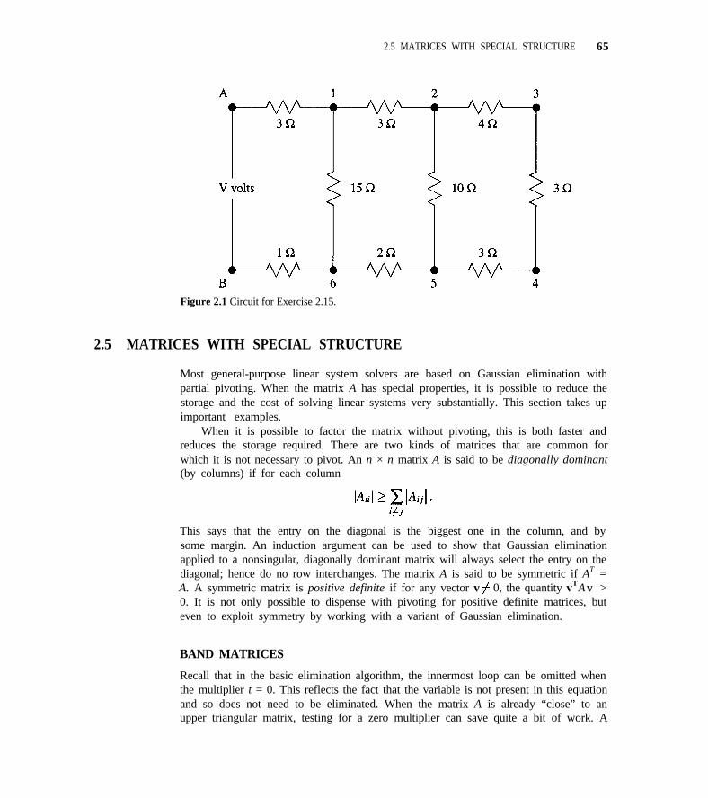
2.5 MATRICES WITH SPECIAL STRUCTURE 65
Figure 2.1 Circuit for Exercise 2.15.
2.5 MATRICES WITH SPECIAL STRUCTURE
Most general-purpose linear system solvers are based on Gaussian elimination withpartial pivoting. When the matrix A has special properties, it is possible to reduce thestorage and the cost of solving linear systems very substantially. This section takes upimportant examples.
When it is possible to factor the matrix without pivoting, this is both faster andreduces the storage required. There are two kinds of matrices that are common forwhich it is not necessary to pivot. An n × n matrix A is said to be diagonally dominant(by columns) if for each column
This says that the entry on the diagonal is the biggest one in the column, and bysome margin. An induction argument can be used to show that Gaussian eliminationapplied to a nonsingular, diagonally dominant matrix will always select the entry on thediagonal; hence do no row interchanges. The matrix A is said to be symmetric if AT =A. A symmetric matrix is positive definite if for any vector v 0, the quantity vTAv >0. It is not only possible to dispense with pivoting for positive definite matrices, buteven to exploit symmetry by working with a variant of Gaussian elimination.
BAND MATRICES
Recall that in the basic elimination algorithm, the innermost loop can be omitted whenthe multiplier t = 0. This reflects the fact that the variable is not present in this equationand so does not need to be eliminated. When the matrix A is already “close” to anupper triangular matrix, testing for a zero multiplier can save quite a bit of work. A
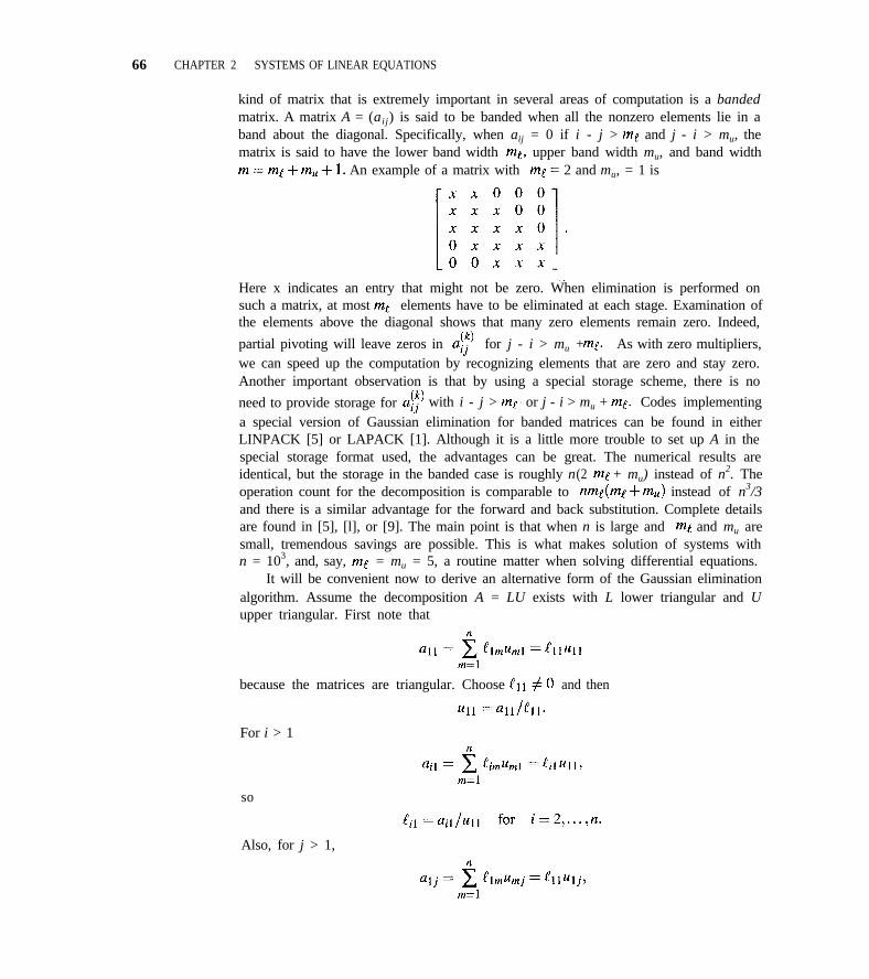
66 CHAPTER 2 SYSTEMS OF LINEAR EQUATIONS
kind of matrix that is extremely important in several areas of computation is a bandedmatrix. A matrix A = (a i j) is said to be banded when all the nonzero elements lie in aband about the diagonal. Specifically, when aij = 0 if i - j > and j - i > mu, thematrix is said to have the lower band width upper band width mu, and band width
An example of a matrix with = 2 and mu, = 1 is
Here x indicates an entry that might not be zero. When elimination is performed onsuch a matrix, at most elements have to be eliminated at each stage. Examination ofthe elements above the diagonal shows that many zero elements remain zero. Indeed,
partial pivoting will leave zeros in for j - i > mu + As with zero multipliers,we can speed up the computation by recognizing elements that are zero and stay zero.Another important observation is that by using a special storage scheme, there is no
need to provide storage for with i - j > or j - i > mu + Codes implementinga special version of Gaussian elimination for banded matrices can be found in eitherLINPACK [5] or LAPACK [1]. Although it is a little more trouble to set up A in thespecial storage format used, the advantages can be great. The numerical results areidentical, but the storage in the banded case is roughly n(2 + mu) instead of n2. Theoperation count for the decomposition is comparable to instead of n3/3and there is a similar advantage for the forward and back substitution. Complete detailsare found in [5], [l], or [9]. The main point is that when n is large and and mu aresmall, tremendous savings are possible. This is what makes solution of systems withn = 103, and, say, = mu = 5, a routine matter when solving differential equations.
It will be convenient now to derive an alternative form of the Gaussian eliminationalgorithm. Assume the decomposition A = LU exists with L lower triangular and Uupper triangular. First note that
because the matrices are triangular. Choose and then
For i > 1
so
Also, for j > 1,
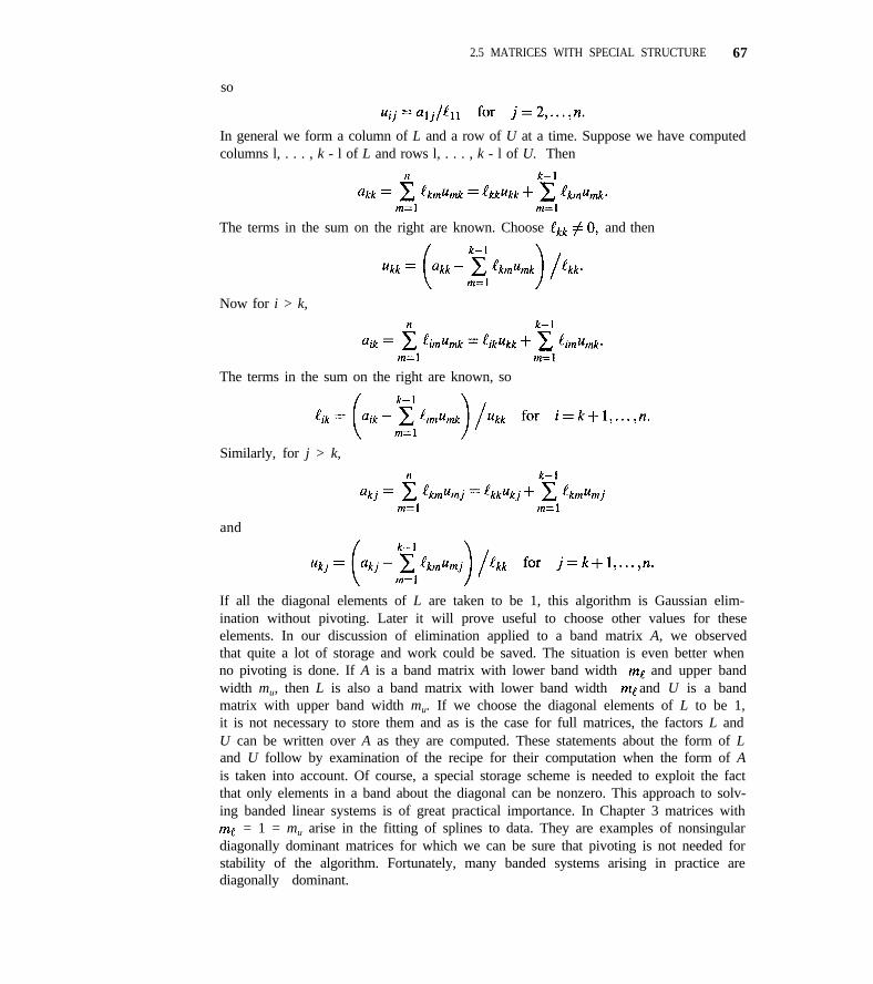
2.5 MATRICES WITH SPECIAL STRUCTURE 67
so
In general we form a column of L and a row of U at a time. Suppose we have computedcolumns l, . . . , k - l of L and rows l, . . . , k - l of U. Then
The terms in the sum on the right are known. Choose and then
Now for i > k,
The terms in the sum on the right are known, so
Similarly, for j > k,
and
If all the diagonal elements of L are taken to be 1, this algorithm is Gaussian elim-ination without pivoting. Later it will prove useful to choose other values for theseelements. In our discussion of elimination applied to a band matrix A, we observedthat quite a lot of storage and work could be saved. The situation is even better whenno pivoting is done. If A is a band matrix with lower band width and upper bandwidth mu, then L is also a band matrix with lower band width and U is a bandmatrix with upper band width mu. If we choose the diagonal elements of L to be 1,it is not necessary to store them and as is the case for full matrices, the factors L andU can be written over A as they are computed. These statements about the form of Land U follow by examination of the recipe for their computation when the form of Ais taken into account. Of course, a special storage scheme is needed to exploit the factthat only elements in a band about the diagonal can be nonzero. This approach to solv-ing banded linear systems is of great practical importance. In Chapter 3 matrices with
= 1 = mu arise in the fitting of splines to data. They are examples of nonsingulardiagonally dominant matrices for which we can be sure that pivoting is not needed forstability of the algorithm. Fortunately, many banded systems arising in practice arediagonally dominant.
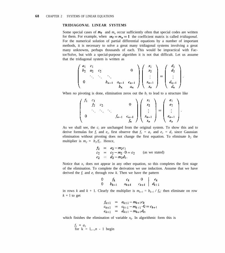
68 CHAPTER 2 SYSTEMS OF LINEAR EQUATIONS
TRIDIAGONAL LINEAR SYSTEMS
Some special cases of and mu occur sufficiently often that special codes are writtenfor them. For example, when the coefficient matrix is called tridiagonal.For the numerical solution of partial differential equations by a number of importantmethods, it is necessary to solve a great many tridiagonal systems involving a greatmany unknowns, perhaps thousands of each. This would be impractical with Fac-tor/Solve, but with a special-purpose algorithm it is not that difficult. Let us assumethat the tridiagonal system is written as
When no pivoting is done, elimination zeros out the bi to lead to a structure like
As we shall see, the ci are unchanged from the original system. To show this and toderive formulas for fi and ei, first observe that f1 = a1 and e1 = d1 since Gaussianelimination without pivoting does not change the first equation. To eliminate b2 themultiplier is m2 = b2/f1. Hence,
(as we stated)
Notice that x1 does not appear in any other equation, so this completes the first stageof the elimination. To complete the derivation we use induction. Assume that we havederived the fi and ei through row k. Then we have the pattern
in rows k and k + 1. Clearly the multiplier is mk+l = bk+l / fk; then eliminate on rowk + l to get
which finishes the elimination of variable xk. In algorithmic form this is
f1 = a1for k = l,...,n - 1 begin
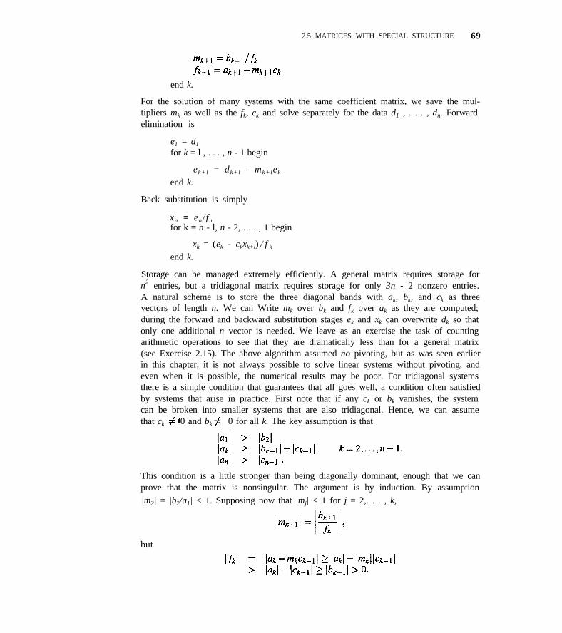
2.5 MATRICES WITH SPECIAL STRUCTURE 69
end k.
For the solution of many systems with the same coefficient matrix, we save the mul-tipliers mk as well as the fk, ck and solve separately for the data d1 , . . . , dn. Forwardelimination is
e1 = d1
for k = l , . . . , n - 1 begin
ek+l = dk+l - mk+lek
end k.
Back substitution is simply
xn = en /fnfor k = n - l, n - 2, . . . , 1 begin
xk = (ek - ckxk+l) / f k
end k.
Storage can be managed extremely efficiently. A general matrix requires storage forn2 entries, but a tridiagonal matrix requires storage for only 3n - 2 nonzero entries.A natural scheme is to store the three diagonal bands with ak, bk, and ck as threevectors of length n. We can Write mk over bk and fk over ak as they are computed;during the forward and backward substitution stages ek and xk can overwrite dk so thatonly one additional n vector is needed. We leave as an exercise the task of countingarithmetic operations to see that they are dramatically less than for a general matrix(see Exercise 2.15). The above algorithm assumed no pivoting, but as was seen earlierin this chapter, it is not always possible to solve linear systems without pivoting, andeven when it is possible, the numerical results may be poor. For tridiagonal systemsthere is a simple condition that guarantees that all goes well, a condition often satisfiedby systems that arise in practice. First note that if any ck or bk vanishes, the systemcan be broken into smaller systems that are also tridiagonal. Hence, we can assumethat ck 0 and bk 0 for all k. The key assumption is that
This condition is a little stronger than being diagonally dominant, enough that we canprove that the matrix is nonsingular. The argument is by induction. By assumption|m2| = |b2/a1| < 1. Supposing now that |mj| < 1 for j = 2,. . . , k,
but
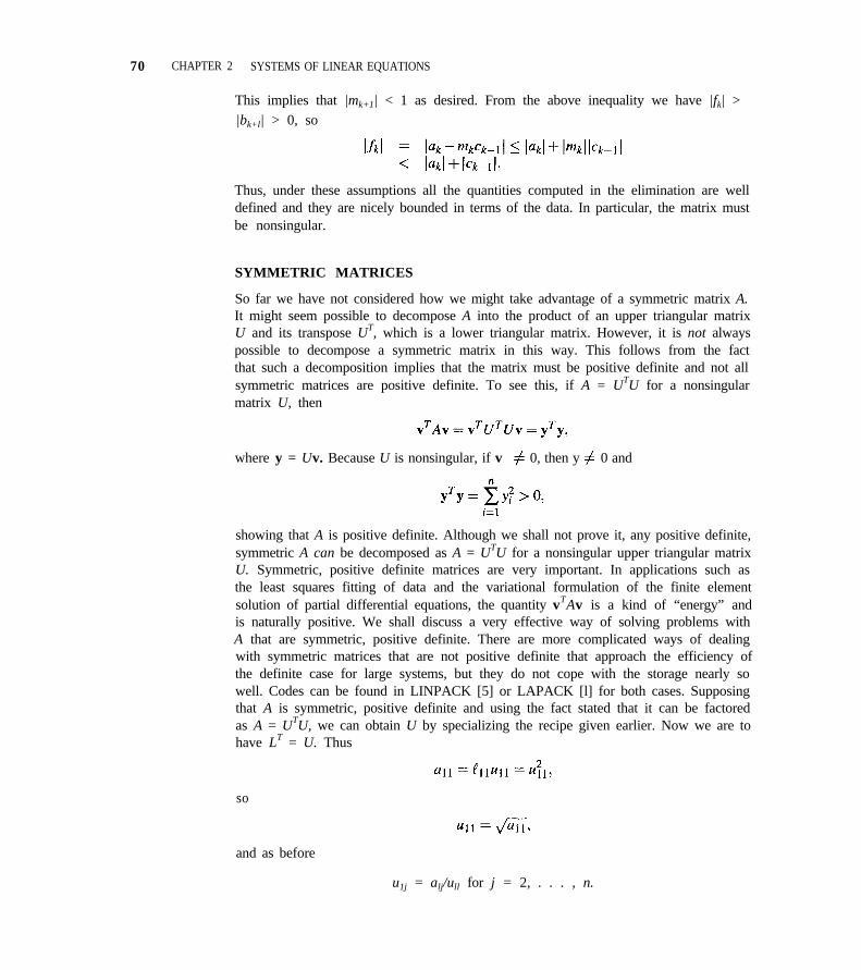
70 CHAPTER 2 SYSTEMS OF LINEAR EQUATIONS
This implies that |mk+1| < 1 as desired. From the above inequality we have |fk| > |bk+l| > 0, so
Thus, under these assumptions all the quantities computed in the elimination are welldefined and they are nicely bounded in terms of the data. In particular, the matrix mustbe nonsingular.
SYMMETRIC MATRICES
So far we have not considered how we might take advantage of a symmetric matrix A.It might seem possible to decompose A into the product of an upper triangular matrixU and its transpose UT, which is a lower triangular matrix. However, it is not alwayspossible to decompose a symmetric matrix in this way. This follows from the factthat such a decomposition implies that the matrix must be positive definite and not allsymmetric matrices are positive definite. To see this, if A = UTU for a nonsingularmatrix U, then
where y = Uv. Because U is nonsingular, if v 0, then y 0 and
showing that A is positive definite. Although we shall not prove it, any positive definite,symmetric A can be decomposed as A = UTU for a nonsingular upper triangular matrixU. Symmetric, positive definite matrices are very important. In applications such asthe least squares fitting of data and the variational formulation of the finite elementsolution of partial differential equations, the quantity vTAv is a kind of “energy” andis naturally positive. We shall discuss a very effective way of solving problems withA that are symmetric, positive definite. There are more complicated ways of dealingwith symmetric matrices that are not positive definite that approach the efficiency ofthe definite case for large systems, but they do not cope with the storage nearly sowell. Codes can be found in LINPACK [5] or LAPACK [l] for both cases. Supposingthat A is symmetric, positive definite and using the fact stated that it can be factoredas A = UTU, we can obtain U by specializing the recipe given earlier. Now we are tohave LT = U. Thus
so
and as before
u1j = alj/ull for j = 2, . . . , n.
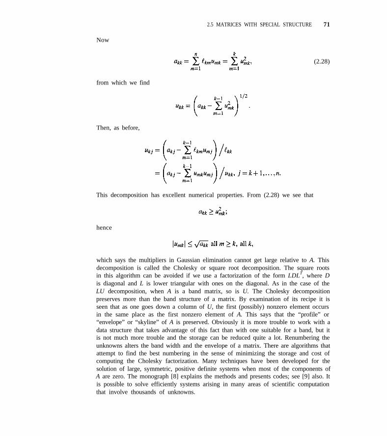
2.5 MATRICES WITH SPECIAL STRUCTURE 71
Now
(2.28)
from which we find
Then, as before,
This decomposition has excellent numerical properties. From (2.28) we see that
hence
which says the multipliers in Gaussian elimination cannot get large relative to A. Thisdecomposition is called the Cholesky or square root decomposition. The square rootsin this algorithm can be avoided if we use a factorization of the form LDLT, where Dis diagonal and L is lower triangular with ones on the diagonal. As in the case of theLU decomposition, when A is a band matrix, so is U. The Cholesky decompositionpreserves more than the band structure of a matrix. By examination of its recipe it isseen that as one goes down a column of U, the first (possibly) nonzero element occursin the same place as the first nonzero element of A. This says that the “profile” or“envelope” or “skyline” of A is preserved. Obviously it is more trouble to work with adata structure that takes advantage of this fact than with one suitable for a band, but itis not much more trouble and the storage can be reduced quite a lot. Renumbering theunknowns alters the band width and the envelope of a matrix. There are algorithms thatattempt to find the best numbering in the sense of minimizing the storage and cost ofcomputing the Cholesky factorization. Many techniques have been developed for thesolution of large, symmetric, positive definite systems when most of the components ofA are zero. The monograph [8] explains the methods and presents codes; see [9] also. Itis possible to solve efficiently systems arising in many areas of scientific computationthat involve thousands of unknowns.
72 CHAPTER 2 SYSTEMS OF LINEAR EQUATIONS
EXERCISES
2.19 Count the arithmetic operations required by the algo-rithm in Section 2.5.2 for a linear system of n equa-tions with a tridiagonal coefficient matrix and m right-
hand sides. Compare this with what is required for ageneral system.
2.6 CASE STUDY 2
All the standard methods of approximating the solution of elliptic partial differentialequations, PDEs, involve the solution of a system of linear equations. The numericalsolution of PDEs is a large subject and there are many books devoted to the solutionof particular classes of problems and to the use of particular kinds of methods. TheGalerkin method is a very important one that we illustrate here with a simple examplefrom [4]. After some preparation, the velocity w(x,y) of the steady flow of a viscousfluid in a duct with square cross section can be found as the solution of
subject to no-slip boundary conditions
w(x,y) = 0 on |x| = 1 and |y| = 1.
The same mathematical problem arises in the torsion of a bar of square cross section.Galerkin methods approximate w(x,y) by an expansion
The choice of the basis functions φj is of fundamental importance. For the examplewe shall use
Notice that each φj satisfies the boundary conditions. Also, the problem is such thatw(x,y) has certain symmetry properties, properties shared by these basis functions.Because the φj reflect well the qualitative behavior of the solution, we can hope to geta reasonable approximation with just a few terms in the expansion. This is a globalGalerkin method because each φj approximates the solution over the entire domain.We shall see in Chapter 3 that approximating functions by piecing together polynomialapproximations over subdomains can be very effective. In the present context the sub-domains are called elements, and a Galerkin method based on piecewise polynomialbasis functions is called a finite element method. In any case, when wN is substitutedinto the differential equation, there is a residual
The idea is to find coefficients aj that make this residual small in some sense. Gen-erally there is a residual arising from boundary conditions, too, but for simplicity we
2.6 CASE STUDY 2 73
discuss only the case of basis functions that satisfy the boundary conditions exactly. Toquantify the notion of being small, we make use of an inner product of two functions
f(X,Y) and g(x,y):
The Galerkin method requires that the residual of the approximation be small in thesense that it is orthogonal to all the basis functions, that is, (φi,R) = 0 for i = 1,. . . , N.If we substitute the expansion into the definition of the residual, this becomes
This is a system of linear equations Ca = b for the coefficients ai, whereand bi = - (φ i, 1). When there is more than one independent variable, it is not soeasy to piece together polynomial approximations over elements so that they connectsmoothly, and it is usual to reduce the order of differentiation in the inner product of Cij
from two to one by means of integration by parts (Green’s theorem). With the globalpolynomial approximation of this example, there is no difficulty forming directly theLaplacian of the basis functions.
In the classic Galerkin method the integrals of the inner products are computedexactly. This is possible for our simple example, but in practice integrals are approxi-mated numerically. A common procedure for general functions is based on Gaussianquadrature. As we shall see in Chapter 5, a Gaussian quadrature formula of M pointsconsists of a set of nodes η i and weights Ai such that
provides the best possible approximation in a certain sense. In particular, the formulais exact for any polynomial u(x) of degree no more than 2M - 1. In Section 5.6 wediscuss how such a formula can be used to obtain an approximation to the integral ofa function of two variables:
Generally M is quite small, but for our example we take it to be 5. The basis functionswe use are polynomials and inspection of the integrands for the cases N = 1, 2, 3that we solve numerically shows that with M = 5, the integrals we need are computedexactly.
Often when solving PDEs, quantities computed from the solution are at least as in-teresting as the solution itself. Such a quantity for this example is the nondimensionalflow rate
The Galerkin approximations computed in the manner described gave
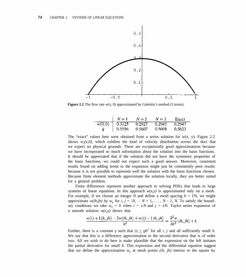
74 CHAPTER 2 SYSTEMS OF LINEAR EQUATIONS
Figure 2.2 The flow rate w(x, 0) approximated by Galerkin’s method (3 terms).
The “exact” values here were obtained from a series solution for w(x, y). Figure 2.2shows w3(x,0), which exhibits the kind of velocity distribution across the duct thatwe expect on physical grounds. These are exceptionally good approximations becausewe have incorporated so much information about the solution into the basis functions.It should be appreciated that if the solution did not have the symmetry properties ofthe basis functions, we could not expect such a good answer. Moreover, consistentresults found on adding terms to the expansion might just be consistently poor resultsbecause it is not possible to represent well the solution with the basis functions chosen.Because finite element methods approximate the solution locally, they are better suitedfor a general problem.
Finite differences represent another approach to solving PDEs that leads to largesystems of linear equations. In this approach w(x,y) is approximated only on a mesh.For example, if we choose an integer N and define a mesh spacing h = l/N, we mightapproximate w(ih,jh) by wij for i, j = -N, - N + 1,. . . , N - 1, N. To satisfy the bound-ary conditions we take wij = 0 when i = ±N and j = ±N. Taylor series expansion ofa smooth solution w(x,y) shows that
Further, there is a constant γ such that |τ| < γh2 for all i, j and all sufficiently small h.We say that this is a difference approximation to the second derivative that is of ordertwo. All we wish to do here is make plausible that the expression on the left imitatesthe partial derivative for small h. This expression and the differential equation suggestthat we define the approximation wij at mesh points (ih, jh) interior to the square by
the equation
2.6 CASE STUDY 2 75
The set of (2N - 1)2 equations can be rewritten as
For this discrete approximation to the PDE to be a reasonable one, the mesh spacing hmust be small, but then we must have a large set of linear equations. It is of the utmostpractical importance that the equations are sparse. Indeed, there are only five nonzerocoefficients in each row of the matrix. Historically such equations were solved by iter-ative methods. The methods used are very simple and self-correcting, so that a mistakedoes not prevent computing the correct answer. Both characteristics are very importantto hand computation. Also important is that the methods require storage only for thenonzero coefficients, the solution itself, and perhaps another vector of the same size asthe solution. For a problem as simple as this example, it is not even necessary to storethe coefficients of the matrix. Iterative methods take advantage of the fact that we donot require an accurate solution. After all, wi,j is only an approximation to w(ih, jh)of modest accuracy, so there is little point to computing it very accurately.
The classic iterative procedures for solving equations like those arising in thisexample are most naturally described in terms of the equation itself. First let us rewritethe equation as
The Jacobi iteration improves an approximation w(k) by computing
for all i, j. This amounts to saying that we define so as to make the residual inequation j equal to zero. This is a very simple and inexpensive iteration that requiresonly storage for the current and next approximations. A refinement suggests itself:
Would it not be better to use instead of for the rest of the computation?Besides, if we do this, we would halve the storage required. This is called the Gauss-Seidel iteration. There is a complication with this method. So far we have not written
out the matrix explicitly, so we have not specified the order of the components
in the vector w(k). If we are to start using as soon as it is computed, the orderin which components are improved matters. ‘A question that arises in the use of anyiterative method is when to quit. A natural way is to measure the residual of the currentsolution and quit when it is less than a tolerance.
For the example we used the Gauss-Seidel iteration and improved the unknownsfrom left to right, bottom to top, that is, for each i = -N + 1,. . . , N - 1, we improvedwi , j for j = -N + l,..., N - 1. We took N = 5, which led to a system of 81 equations
for unknowns at points interior to the region. It was convenient to start with
for all i, j. With a tolerance of 5 × 10⁻⁴, convergence was achieved in 89 iterations.
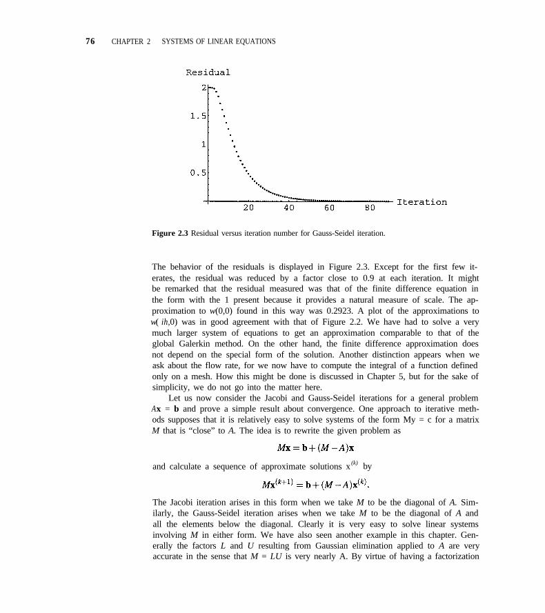
76 CHAPTER 2 SYSTEMS OF LINEAR EQUATIONS
Figure 2.3 Residual versus iteration number for Gauss-Seidel iteration.
The behavior of the residuals is displayed in Figure 2.3. Except for the first few it-erates, the residual was reduced by a factor close to 0.9 at each iteration. It mightbe remarked that the residual measured was that of the finite difference equation inthe form with the 1 present because it provides a natural measure of scale. The ap-proximation to w(0,0) found in this way was 0.2923. A plot of the approximations tow( ih,0) was in good agreement with that of Figure 2.2. We have had to solve a verymuch larger system of equations to get an approximation comparable to that of theglobal Galerkin method. On the other hand, the finite difference approximation doesnot depend on the special form of the solution. Another distinction appears when weask about the flow rate, for we now have to compute the integral of a function definedonly on a mesh. How this might be done is discussed in Chapter 5, but for the sake ofsimplicity, we do not go into the matter here.
Let us now consider the Jacobi and Gauss-Seidel iterations for a general problemAx = b and prove a simple result about convergence. One approach to iterative meth-ods supposes that it is relatively easy to solve systems of the form My = c for a matrixM that is “close” to A. The idea is to rewrite the given problem as
and calculate a sequence of approximate solutions x (k) by
The Jacobi iteration arises in this form when we take M to be the diagonal of A. Sim-ilarly, the Gauss-Seidel iteration arises when we take M to be the diagonal of A andall the elements below the diagonal. Clearly it is very easy to solve linear systemsinvolving M in either form. We have also seen another example in this chapter. Gen-erally the factors L and U resulting from Gaussian elimination applied to A are veryaccurate in the sense that M = LU is very nearly A. By virtue of having a factorization
2.6 CASE STUDY 2 77
of this M, it is easy to compute the iterates by forward and back substitution in theusual fashion. With this choice of M, the iteration is the iterative refinement discussedin Section 2.3.2.
Passing to the limit on both sides of the equation defining the iteration, we see thatif the approximations converge at all, they must converge to x. A little manipulationof the equations for x and x(k+1) shows that error e(k) = x - x(k) satisfies
This then implies that
If the number this inequality implies that the process con-
verges for any starting guess x(0). The error decreases by a factor of ρ at each iteration,so if M is close to A in the sense that ρ is small, the process converges quickly. Noticethat the crucial quantity ρ is a kind of relative error of the approximation of A by M.Sharp convergence results are known, but they are beyond the scope of this book; see,for example, [2] or [10].
The situation with iterative refinement is special because we want a very accuratevalue for x. For reasons taken up in Chapter 1, it would be better then to compute theiterate by means of the difference of successive iterates, Thisleads to the form suggested in Section 2.3.2,
Although we have not provided all the details, it is not surprising that even whenA is extraordinarily ill-conditioned, M is sufficiently close to A that the result justestablished guarantees convergence.
The Jacobi iteration is more easily understood by looking at components. Equa-tion j is
A little manipulation results in
We cannot expect this iteration to work unless the entries off the diagonal of A are smallcompared to those on the diagonal. To obtain a sufficient condition for convergence,let us suppose that A is strictly diagonally dominant by rows, meaning that there is anumber ρ < 1 such that for all j,
78 CHAPTER 2 SYSTEMS OF LINEAR EQUATIONS
A little calculation shows that the error
This holds for each j, so
telling us that the worst error is reduced by a factorlarge system of linear equations arises in Chapter 3splines. Equation j has the form
of ρ at each iteration. A (possibly)when fitting data by smooth cubic
and the first and last equations have the form
2hlxl + hl = bl
hn-lxn-l + 2hnxn = bn.
The quantities hj appearing in these equations are all positive. Evidently this system ofequations is strictly diagonally dominant by rows with ρ = l/2. The Jacobi iterationwould be a reasonable way to solve these systems, but A is a symmetric tridiagonalmatrix and the special version of elimination from Section 2.5.2 is so effective thatthere is little point to iterative methods. In components the Gauss-Seidel iteration is
A modification of the proof given for the Jacobi iteration shows that this iteration alsoconverges whenever A is strictly diagonally dominant by rows. The finite differenceequations of the example do not satisfy the convergence criterion just developed, butthey do have a kind of diagonal dominance for which it is possible to prove conver-gence of both the Jacobi and Gauss-Seidel methods.
The Jacobi iteration and the Gauss-Seidel iteration are too slow to be practical formost problems arising in practice. However, they are still important as preconditionersfor more elaborate iterative procedures. For more information about iterative methods,see [2] or [10]. The latter provides some substantial applications to the numericalsolution of PDEs.
REFERENCES
1. E. Anderson, et al., LAPACK User’s Guide, SIAM, Philadelphia, 1992.
2. O. Axelsson, Iterative Solution Methods, Cambridge University Press, New York, 1994.
3. A. Cline, C. Moler, G. Stewart, and J. Wilkinson, “An estimate for the condition number of amatrix,” SIAM J. Numer. Anal., 16 (1979), pp. 368-375.
4. C. A. J. Fletcher, Computational Galerkin Methods, Springer-Verlag, New York, 1984.
5. J, Dongarra, J. Bunch, C. Moler, and G. Stewart, LINPACK User’s Guide, SIAM, Philadelphia,1979.
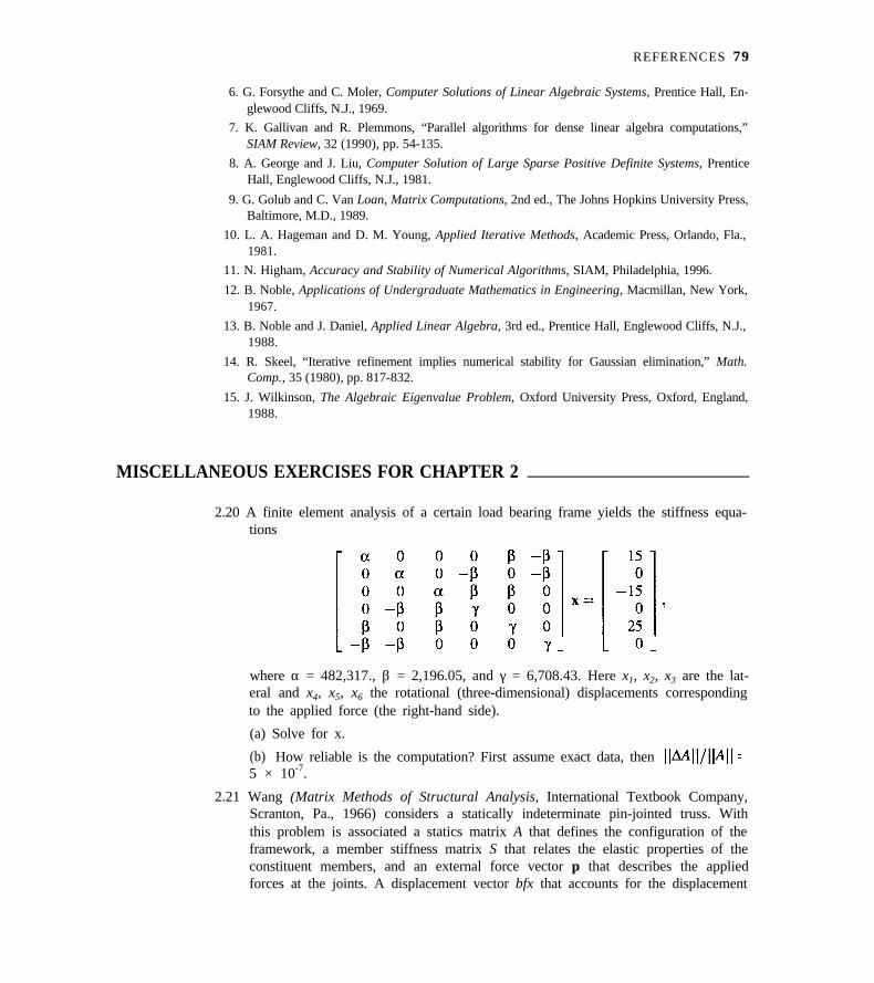
REFERENCES 79
6. G. Forsythe and C. Moler, Computer Solutions of Linear Algebraic Systems, Prentice Hall, En-glewood Cliffs, N.J., 1969.
7. K. Gallivan and R. Plemmons, “Parallel algorithms for dense linear algebra computations,”SIAM Review, 32 (1990), pp. 54-135.
8. A. George and J. Liu, Computer Solution of Large Sparse Positive Definite Systems, PrenticeHall, Englewood Cliffs, N.J., 1981.
9. G. Golub and C. Van Loan, Matrix Computations, 2nd ed., The Johns Hopkins University Press,Baltimore, M.D., 1989.
10. L. A. Hageman and D. M. Young, Applied Iterative Methods, Academic Press, Orlando, Fla.,1981.
11. N. Higham, Accuracy and Stability of Numerical Algorithms, SIAM, Philadelphia, 1996.
12. B. Noble, Applications of Undergraduate Mathematics in Engineering, Macmillan, New York,1967.
13. B. Noble and J. Daniel, Applied Linear Algebra, 3rd ed., Prentice Hall, Englewood Cliffs, N.J.,1988.
14. R. Skeel, “Iterative refinement implies numerical stability for Gaussian elimination,” Math.Comp., 35 (1980), pp. 817-832.
15. J. Wilkinson, The Algebraic Eigenvalue Problem, Oxford University Press, Oxford, England,1988.
MISCELLANEOUS EXERCISES FOR CHAPTER 2
2.20 A finite element analysis of a certain load bearing frame yields the stiffness equa-tions
where α = 482,317., β = 2,196.05, and γ = 6,708.43. Here x1, x2, x3 are the lat-eral and x4, x5, x6 the rotational (three-dimensional) displacements correspondingto the applied force (the right-hand side).
(a) Solve for x.
(b) How reliable is the computation? First assume exact data, then5 × 10-7.
2.21 Wang (Matrix Methods of Structural Analysis, International Textbook Company,Scranton, Pa., 1966) considers a statically indeterminate pin-jointed truss. Withthis problem is associated a statics matrix A that defines the configuration of theframework, a member stiffness matrix S that relates the elastic properties of theconstituent members, and an external force vector p that describes the appliedforces at the joints. A displacement vector bfx that accounts for the displacement

80 CHAPTER 2 SYSTEMS OF LINEAR EQUATIONS
2.22
at each degree of freedom and an internal force vector f acting on each membersatisfies
For one example
The matrix S has all zero entries except along the diagonal where the entries are
{4800: 10000, 4800, 10000, 10000, 10000, 3000, 4800, 4800, 3000}.
Write a program to form matrix products and determine the elements of K. Solvefor x using the three p vectors
Find the corresponding vectors f.
This exercise assumes a familiarity with matrix multiplication. An appropriateorganization of Gaussian elimination as in Factor/Solve makes it efficient to solvesystems of equations with different right-hand sides but the same coefficient ma-trix A. It is more complicated to deal with changes in A, but a formula called theSherman-Morrison formula makes it possible to deal with certain modificationsefficiently. Assume that we have already factored A into LU and we want to solve(A + uvT)x = b for given column vectors u, v, and b. Show that this can be doneby first solving AZ = u and Ay = b, then forming
A proper choice of u and v handles the change of one row or one column of A.For example, if row i of A is to be changed by adding to it a given row vector vT,just take the column vector u to be zero in all entries except the ith, which is 1.
(a) How do you change column j in A so as to add a given column vector u ?
(b) How do you choose u and v in order to change aij into aij + δ?
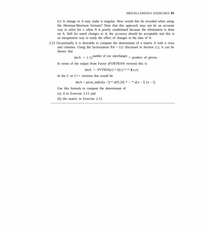
MISCELLANEOUS EXERCISES 81
(c) A change in A may make it singular. How would this be revealed when usingthe Sherman-Morrison formula? Note that this approach may not be an accurateway to solve for x when A is poorly conditioned because the elimination is doneon A. Still for small changes to A, the accuracy should be acceptable and this isan inexpensive way to study the effect of changes to the data of A.
2.23 Occasionally it is desirable to compute the determinant of a matrix A with n rowsand columns. Using the factorization PA = LU discussed in Section 2.2, it can beshown that
detA = (-1) number of row interchanges × product of pivots.
In terms of the output from Factor (FORTRAN version) this is
detA = PVTIDX(n) * A(l,1) *···* A( n,n).
In the C or C++ versions this would be
detA = pivot_index[n - l] * a[0] [0] * ··· * a[n - l] [n - l].
Use this formula to compute the determinant of
(a) A in Exercise 2.13 and
(b) the matrix in Exercise 2.15.
CHAPTER 3
INTERPOLATION
Often we need to approximate a function f(x) by another “more convenient” functionF(x). This arises in physical processes where f(x) is known only through its valuesat certain sample points x and F(x) is needed to approximate maximum or minimumvalues, to estimate integrals or derivatives, or merely to generate values for f(x) atpoints where experimental data are not available. This also arises when f(x) is knownbut is difficult to evaluate, integrate, or differentiate. A familiar example is the functionf(x) = sinx that has to be approximated in a way that can be evaluated by calculatorsand computers. This is a fundamental principle of numerical analysis: if we cannotcarry out a basic computation with the function of interest, we approximate it by afunction for which we can do the computation.
In this chapter a function f(x) is approximated by an interpolant F(x), a functionthat agrees with f(x) at certain points. A formal definition of the verb interpolate is asfollows.
Definition. interpolation: A function F(x) is said to interpolate f(x) at thepoints {x l , . . . ,xN) if
F(x j) = f(x j), j = 1,2 ,..., N.
The process of constructing such a function F(x) is called interpolation.
There are many types of approximating functions F(x) and which one to use de-pends to a large extent on the nature of the data and the intended use of the approxima-tion. Perhaps the simplest approximating functions are polynomials. It can be shownthat any continuous function can be approximated arbitrarily well over a finite inter-val by a polynomial. More to the point, polynomials and their ratios (called rationalfunctions) are the only functions that can be evaluated directly on a computer. Forthis reason polynomials are used not only for interpolation but also as a foundation formost of the methods in the remaining chapters of the book. Polynomial splines, that is,piecewise polynomial functions, are a very powerful tool for approximating functionsand are the main object of study in this chapter. In many applications the appearanceof the graph of F(x) is of great importance. For this reason it is very helpful to havea graphing package for visualization of the approximating functions derived in thischapter.
82
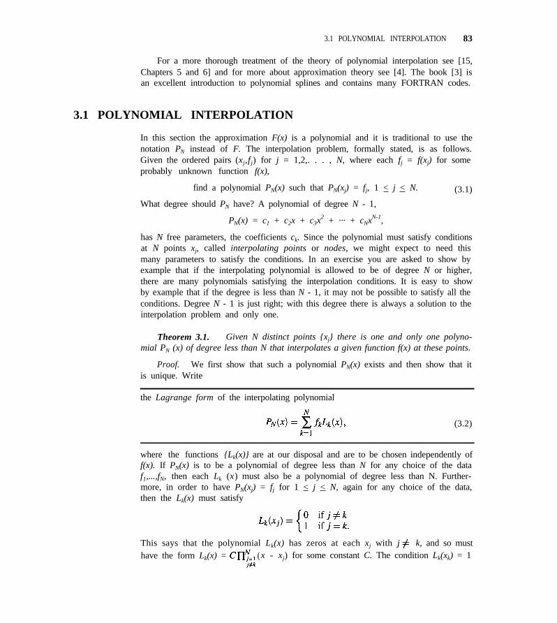
3.1 POLYNOMIAL INTERPOLATION 83
For a more thorough treatment of the theory of polynomial interpolation see [15,Chapters 5 and 6] and for more about approximation theory see [4]. The book [3] isan excellent introduction to polynomial splines and contains many FORTRAN codes.
3.1 POLYNOMIAL INTERPOLATION
In this section the approximation F(x) is a polynomial and it is traditional to use thenotation PN instead of F. The interpolation problem, formally stated, is as follows.Given the ordered pairs (xj,fj) for j = 1,2,. . . , N, where each fj = f(xj) for someprobably unknown function f(x),
find a polynomial PN(x) such that PN(xj) = fj, 1 < j < N.
What degree should PN have? A polynomial of degree N - 1,
(3.1)
PN(x) = c1 + c2x + c3x2 + ··· + cNxN-1,
has N free parameters, the coefficients ck. Since the polynomial must satisfy conditionsat N points xj, called interpolating points or nodes, we might expect to need thismany parameters to satisfy the conditions. In an exercise you are asked to show byexample that if the interpolating polynomial is allowed to be of degree N or higher,there are many polynomials satisfying the interpolation conditions. It is easy to showby example that if the degree is less than N - 1, it may not be possible to satisfy all theconditions. Degree N - 1 is just right; with this degree there is always a solution to theinterpolation problem and only one.
Theorem 3.1. Given N distinct points {xj} there is one and only one polyno-mial PN (x) of degree less than N that interpolates a given function f(x) at these points.
Proof. We first show that such a polynomial PN(x) exists and then show that itis unique. Write
the Lagrange form of the interpolating polynomial
(3.2)
where the functions {Lk(x)} are at our disposal and are to be chosen independently off(x). If PN(x) is to be a polynomial of degree less than N for any choice of the dataf1,...,fN, then each Lk (x) must also be a polynomial of degree less than N. Further-more, in order to have PN(xj) = fj for 1 < j < N, again for any choice of the data,then the Lk(x) must satisfy
This says that the polynomial Lk(x) has zeros at each xj with j k, and so musthave the form Lk(x) = (x - xj) for some constant C. The condition Lk(xk) = 1
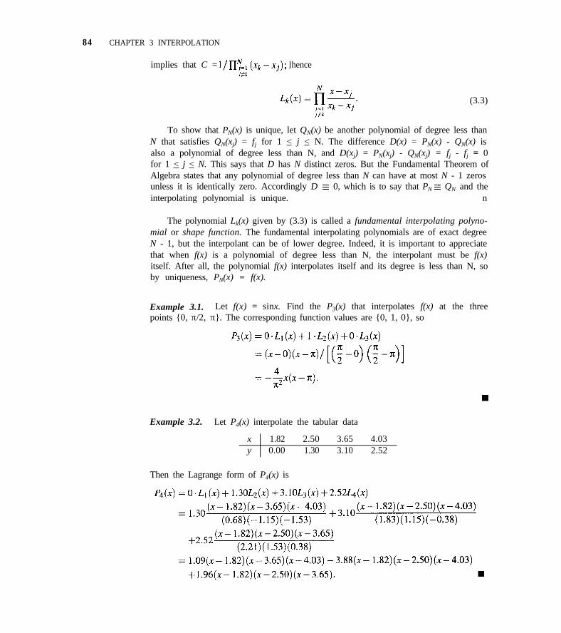
84 CHAPTER 3 INTERPOLATION
implies that C = hence
(3.3)
To show that PN(x) is unique, let QN(x) be another polynomial of degree less thanN that satisfies QN(xj) = fj for 1 < j < N. The difference D(x) = PN(x) - QN(x) isalso a polynomial of degree less than N, and D(xj) = PN(xj) - QN(xj) = fj - fj = 0for 1 < j < N. This says that D has N distinct zeros. But the Fundamental Theorem ofAlgebra states that any polynomial of degree less than N can have at most N - 1 zerosunless it is identically zero. Accordingly D 0, which is to say that PN QN and theinterpolating polynomial is unique. n
The polynomial Lk(x) given by (3.3) is called a fundamental interpolating polyno-mial or shape function. The fundamental interpolating polynomials are of exact degreeN - 1, but the interpolant can be of lower degree. Indeed, it is important to appreciatethat when f(x) is a polynomial of degree less than N, the interpolant must be f(x)itself. After all, the polynomial f(x) interpolates itself and its degree is less than N, soby uniqueness, PN(x) = f(x).
Example 3.1. Let f(x) = sinx. Find the P3(x) that interpolates f(x) at the threepoints {0, π/2, π}. The corresponding function values are {0, 1, 0}, so
Example 3.2. Let P4(x) interpolate the tabular data
x 1.82 2.50 3.65 4.03y 0.00 1.30 3.10 2.52
Then the Lagrange form of P4(x) is
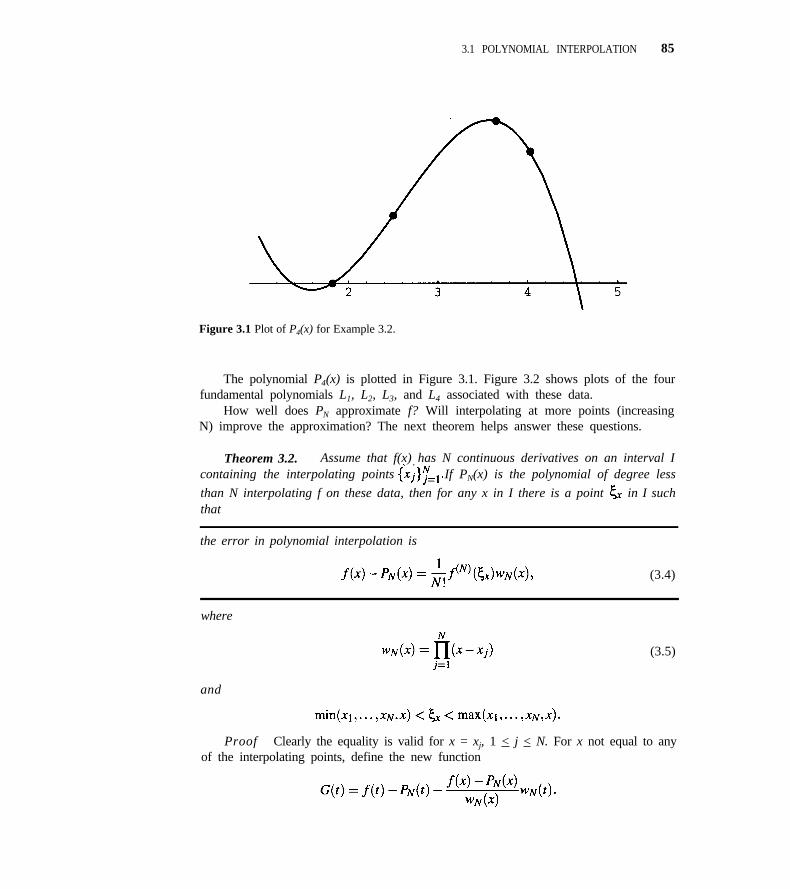
3.1 POLYNOMIAL INTERPOLATION 85
Figure 3.1 Plot of P4(x) for Example 3.2.
The polynomial P4(x) is plotted in Figure 3.1. Figure 3.2 shows plots of the fourfundamental polynomials L1, L2, L3, and L4 associated with these data.
How well does PN approximate f? Will interpolating at more points (increasingN) improve the approximation? The next theorem helps answer these questions.
Theorem 3.2. Assume that f(x) has N continuous derivatives on an interval Icontaining the interpolating points If PN(x) is the polynomial of degree less
than N interpolating f on these data, then for any x in I there is a point in I suchthat
the error in polynomial interpolation is
(3.4)
where
(3.5)
and
Proof Clearly the equality is valid for x = xj, 1 < j < N. For x not equal to anyof the interpolating points, define the new function
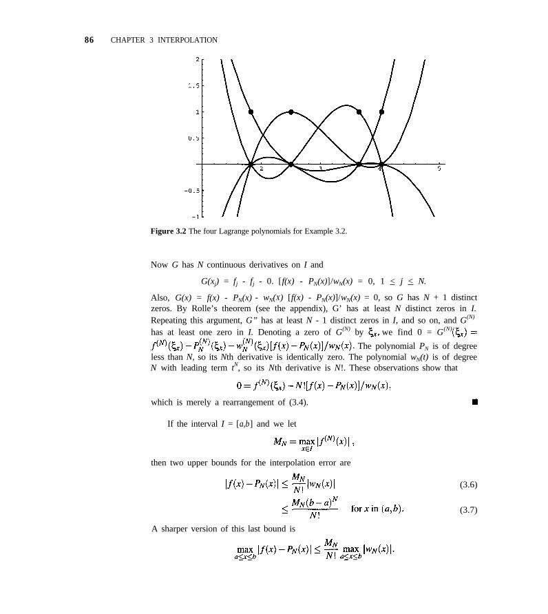
86 CHAPTER 3 INTERPOLATION
Figure 3.2 The four Lagrange polynomials for Example 3.2.
Now G has N continuous derivatives on I and
G(xj) = fj - fj - 0. [f(x) - PN(x)]/wN(x) = 0, 1 < j < N.
Also, G(x) = f(x) - PN(x) - wN(X) [f(x) - PN(x)]/wN(x) = 0, so G has N + 1 distinctzeros. By Rolle’s theorem (see the appendix), G’ has at least N distinct zeros in I.Repeating this argument, G” has at least N - 1 distinct zeros in I, and so on, and G(N)
has at least one zero in I. Denoting a zero of G(N) by we find 0 = G(N)
The polynomial PN is of degreeless than N, so its Nth derivative is identically zero. The polynomial wN(t) is of degreeN with leading term tN, so its Nth derivative is N!. These observations show that
which is merely a rearrangement of (3.4).
If the interval I = [a,b] and we let
then two upper bounds for the interpolation error are
A sharper version of this last bound is
(3.6)
(3.7)
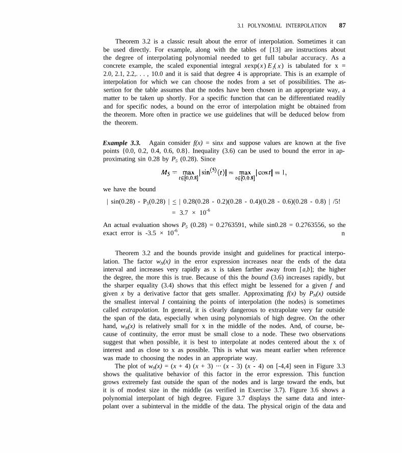
3.1 POLYNOMIAL INTERPOLATION 87
Theorem 3.2 is a classic result about the error of interpolation. Sometimes it canbe used directly. For example, along with the tables of [13] are instructions aboutthe degree of interpolating polynomial needed to get full tabular accuracy. As aconcrete example, the scaled exponential integral xexp(x ) E1( x ) is tabulated for x =2.0, 2.1, 2.2,. . . , 10.0 and it is said that degree 4 is appropriate. This is an example ofinterpolation for which we can choose the nodes from a set of possibilities. The as-sertion for the table assumes that the nodes have been chosen in an appropriate way, amatter to be taken up shortly. For a specific function that can be differentiated readilyand for specific nodes, a bound on the error of interpolation might be obtained fromthe theorem. More often in practice we use guidelines that will be deduced below fromthe theorem.
Example 3.3. Again consider f(x) = sinx and suppose values are known at the fivepoints {0.0, 0.2, 0.4, 0.6, 0.8}. Inequality (3.6) can be used to bound the error in ap-proximating sin 0.28 by P5 (0.28). Since
we have the bound
| sin(0.28) - P5(0.28) | < | 0.28(0.28 - 0.2)(0.28 - 0.4)(0.28 - 0.6)(0.28 - 0.8) | /5!
= 3.7 × 10⁻⁶
An actual evaluation shows P5 (0.28) = 0.2763591, while sin0.28 = 0.2763556, so theexact error is -3.5 × 10⁻⁶. n
Theorem 3.2 and the bounds provide insight and guidelines for practical interpo-lation. The factor wN(x) in the error expression increases near the ends of the datainterval and increases very rapidly as x is taken farther away from [a,b]; the higherthe degree, the more this is true. Because of this the bound (3.6) increases rapidly, butthe sharper equality (3.4) shows that this effect might be lessened for a given f andgiven x by a derivative factor that gets smaller. Approximating f(x) by PN(x) outsidethe smallest interval I containing the points of interpolation (the nodes) is sometimescalled extrapolation. In general, it is clearly dangerous to extrapolate very far outsidethe span of the data, especially when using polynomials of high degree. On the otherhand, wN(x) is relatively small for x in the middle of the nodes. And, of course, be-cause of continuity, the error must be small close to a node. These two observationssuggest that when possible, it is best to interpolate at nodes centered about the x ofinterest and as close to x as possible. This is what was meant earlier when referencewas made to choosing the nodes in an appropriate way.
The plot of w9(x) = (x + 4) (x + 3) ··· (x - 3) (x - 4) on [-4,4] seen in Figure 3.3shows the qualitative behavior of this factor in the error expression. This functiongrows extremely fast outside the span of the nodes and is large toward the ends, butit is of modest size in the middle (as verified in Exercise 3.7). Figure 3.6 shows apolynomial interpolant of high degree. Figure 3.7 displays the same data and inter-polant over a subinterval in the middle of the data. The physical origin of the data and
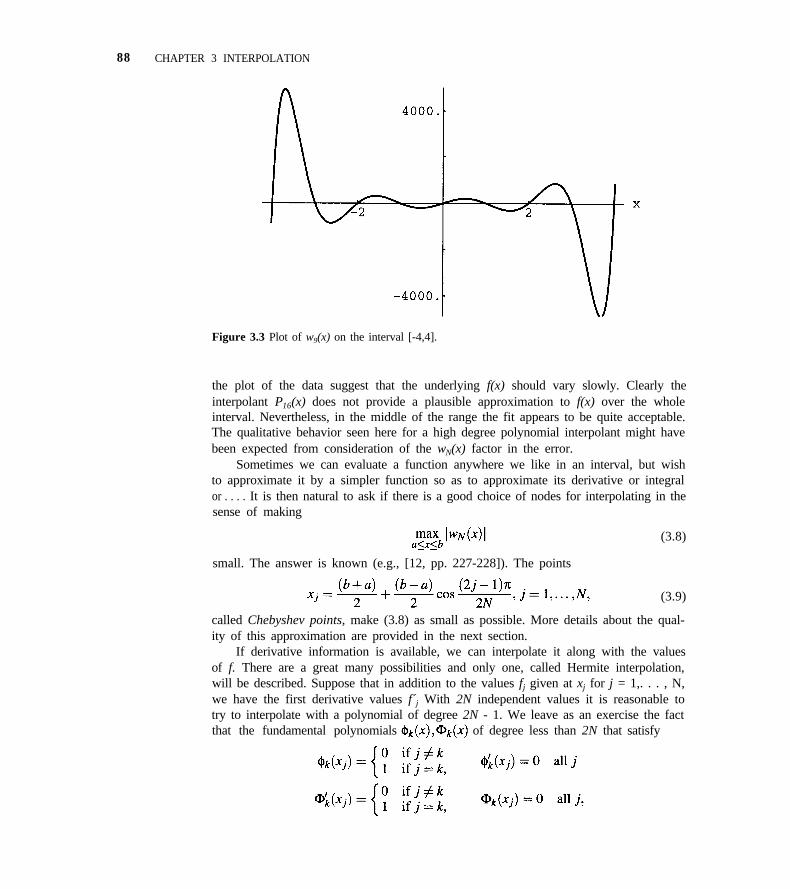
88 CHAPTER 3 INTERPOLATION
Figure 3.3 Plot of w9(x) on the interval [-4,4].
the plot of the data suggest that the underlying f(x) should vary slowly. Clearly theinterpolant P16(x) does not provide a plausible approximation to f(x) over the wholeinterval. Nevertheless, in the middle of the range the fit appears to be quite acceptable.The qualitative behavior seen here for a high degree polynomial interpolant might havebeen expected from consideration of the wN(x) factor in the error.
Sometimes we can evaluate a function anywhere we like in an interval, but wishto approximate it by a simpler function so as to approximate its derivative or integralor . . . . It is then natural to ask if there is a good choice of nodes for interpolating in thesense of making
small. The answer is known (e.g., [12, pp. 227-228]). The points
(3.8)
(3.9)
called Chebyshev points, make (3.8) as small as possible. More details about the qual-ity of this approximation are provided in the next section.
If derivative information is available, we can interpolate it along with the valuesof f. There are a great many possibilities and only one, called Hermite interpolation,will be described. Suppose that in addition to the values fj given at xj for j = 1,. . . , N,we have the first derivative values f´j With 2N independent values it is reasonable totry to interpolate with a polynomial of degree 2N - 1. We leave as an exercise the factthat the fundamental polynomials of degree less than 2N that satisfy
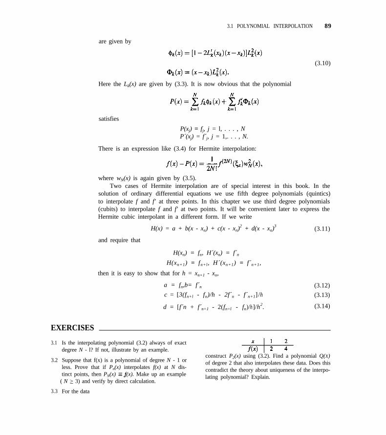
3.1 POLYNOMIAL INTERPOLATION 89
are given by
(3.10)
Here the Lk(x) are given by (3.3). It is now obvious that the polynomial
satisfies
P(xj) = fj, j = l, . . . , NP´(xj) = f´j, j = 1,. . . , N.
There is an expression like (3.4) for Hermite interpolation:
where wN(x) is again given by (3.5).Two cases of Hermite interpolation are of special interest in this book. In the
solution of ordinary differential equations we use fifth degree polynomials (quintics)to interpolate f and f' at three points. In this chapter we use third degree polynomials(cubits) to interpolate f and f' at two points. It will be convenient later to express theHermite cubic interpolant in a different form. If we write
H(x) = a + b(x - xn) + c(x - xn)2 + d(x - xn)
3 (3.11)
and require that
H(xn) = fn, H´(xn) = f´n
H(xn+1) = fn+l, H´(xn+1) = f´n+1,
then it is easy to show that for h = xn+1 - xn,
a = fn,b= f´n
c = [3(fn+l - fn)/h - 2f´n - f´n+1] /h
d = [f´n + f´n+1 - 2(fn+l - fn)/h]/h2.
(3.12)
(3.13)
(3.14)
EXERCISES
3.1
3.2
3.3
Is the interpolating polynomial (3.2) always of exactdegree N - l? If not, illustrate by an example.
Suppose that f(x) is a polynomial of degree N - 1 orless. Prove that if Pn(x) interpolates f(x) at N dis-tinct points, then PN(x) f(x). Make up an example
( N > 3) and verify by direct calculation.
For the data
construct P2(x) using (3.2). Find a polynomial Q(X)of degree 2 that also interpolates these data. Does thiscontradict the theory about uniqueness of the interpo-lating polynomial? Explain.
90 CHAPTER 3 INTERPOLATION
3.4 An alternate method for computing PN(x) is to write
PN(x) = cl + c2x + c3x2 + ··· + cNxN-l .
Then the interpolation conditions, PN(xi) = fi for1 < i < N, yield a system of N equations in the Nunknowns c1, c2, . . . , cN that can be solved using thecodes Factor/Solve. Unfortunately, there are two dif-ficulties with this method: (1) it is expensive (N3/3multiplications), and (2) the coefficient matrix can bevery ill-conditioned.
(a) Implement this algorithm.
(b) Test it on the data in Example 3.5. Use thesame six interpolating values and evaluate (see Exer-cise 3.5) at the remaining points. What is COND?How do the answers compare with those in the textfor&(x) computed by another method?
3.5 There arc several ways to evaluate PN(x) = c1 + c2x +··· + cNxN-1. As a first algorithm we could use
P:= c1
for i = 2, 3, . . . , N begin
P : = P + c i * x i - l
end i.
How many multiplications does this algorithm re-quire? A better approach is based on the nested formof PN(x) used in Section 3.3:
c1 + x{ c2 + x[ c3 + x ( c4 + ··· + cNx) ··· ]}.
For example,
3 + 4x - 6x2+ 5x3 = 3 + x[4 + x(-6 + 5x)].
The new algorithm is
P : = c N
for i = N - l, N - 2, . . . , 1 begin
P: = P * x + ci
end i.
Compare the number of multiplications for this algo-rithm to those for the first one.
3.6 Use the algorithm suggested by Exercise 3.4 to com-pute P12(w), which interpolates all the data in Exam-ple 3.5. Plot P12(w) for 5 < w < 100. Does it lookreasonable?
3.7 Verify the plot in Figure 3.3 of w9(x) to see thatit has smallest magnitude near the middle of thedata. Choose xi = -5 + i and evaluate w9(x) at{±0.5, ±1.5 , . . . ,±4.5, ±5 ±4.5, ±5}.
3.8 Derivatives of f(x) can be estimated by the corre-sponding derivative of PN(x) for some choice of N and
The usual approach is to try
Since PN(x) has degree at most N - 1, mustbe a constant function (i.e., independent of x) .
(a) Use (3.2) to show that
(b) What approximation to f’(x) results when N = 2?
3.9 Verify that the functions given in (3.10) have the fun-damental interpolation properties claimed.
3.10 Derive equations (3.12)-(3.14). Start with
and then derive and solve the four equations for a, b, c,and d resulting from the conditions
3.2 MORE ERROR BOUNDS
Far more can be said about the error in polynomial interpolation. In this section someuseful results are discussed and some results are given for the error made in approxi-mating derivatives by derivatives of an interpolating polynomial.
One way to measure how well PN(x) approximates f(x) on an interval [a, b] is bythe worst error:
3.2 MORE ERROR BOUNDS 91
A fundamental theorem due to Weierstrass (see [4]) states that any function f(x) con-tinuous on a finite interval [a,b] can be approximated arbitrarily well by a polynomial.Stated formally, given any ε > 0, there is a polynomial P(X) such that ||f - P|| < ε. Itis plausible that interpolating f at more and more points in [a,b] would lead to a betterand better approximation. The bound (3.7) shows that if MN does not grow too fast as
the interpolants PN approximate f arbitrarily well. Unfortunately, this is nottrue for all continuous f. A result due to Faber says that for any given set of nodes
in [a,b], there is a function f(x) continuous on [a,b] such thatthe interpolants PN(x) of degree less than N defined by
do not even have ||f - PN|| bounded as Runge’s function
(3.15)
on [-5,5] is a classic example. It seems obvious that interpolating such a smoothfunction at more and more equally spaced points should lead to convergence, but itis found that for even modest N, the interpolants are completely unacceptable (seeExercise 3.11).
It turns out that if one can interpolate at the good nodes (3.9), interpolation is aboutas good a way to approximate f(x) by a low degree polynomial as possible. In fact,Runge’s function can be quite accurately approximated by a polynomial that interpo-lates at the Chebyshev points (see Exercise 3.12). In general, there is a polynomial
of degree less than N that is the best approximation to f(x) on [a, b] in the sense
that provides the smallest value of ||f - P|| for all polynomials P of degreeless than N. Let PN(x) interpolate f(x) at the nodes x1,. . . ,xN in [ a,b]. For any x,
Now is a polynomial of degree less than N, so
because Lagrangian interpolation at N points is exact for such polynomials. Using thefact that PN(xk) = fk, we then find that
and then
92 CHAPTER 3 INTERPOLATION
This inequality relates the error of PN to the error of the best possible polynomialby a factor
which is given in terms of the points of interpolation alone. A simple analytical boundfor the particular nodes (3.9) is found in [17]:
The surprising thing is that the bound is so small for moderate degrees N. For N < 20,it is less than 4. Thus
for all N < 20. These easily constructed interpolating polynomials are, then, about asgood as possible.
Interpolation is not so effective when the nodes cannot be chosen, and as Faber’stheorem suggests, high order interpolation can be quite unsatisfactory. It is common inpractice that a high order interpolating polynomial exhibits large amplitude oscillationseven when the data appear to come from a smooth function f(x). Examples are givenin the next section; for extreme examples the reader need only try interpolating the datain Exercises 3.22, 3.23, and 3.26 by polynomials. For these reasons data are usuallyfit with relatively low degree polynomials, and a variety of devices are used to preventoscillations. Some of these are studied in Section 3.5.
Polynomial interpolation is a basic tool in numerical analysis. As an example,derivatives of an interpolant PN(x) to f(x) can be used to approximate derivatives off(n). An argument very similar to that of Theorem 3.2 (see [15, pp. 289-290] fordetails) can be used to show that for any r < N
where the points are known to be distinct and to satisfy
The point depends on x and lies in the same interval I as the in Theorem 3.2. Ithas been assumed here that xl < x2 < ··· < xN. As a consequence,
(3.16)
as long as xl < x < xN. The Lagrange form of the interpolating polynomial is conve-nient for deriving formulas for numerical differentiation. To approximate a derivativeof f(x) at a point z, given values fk at points {x1, . . . ,xN}, we simply form the inter-polant, differentiate it, and evaluate it at x = z:
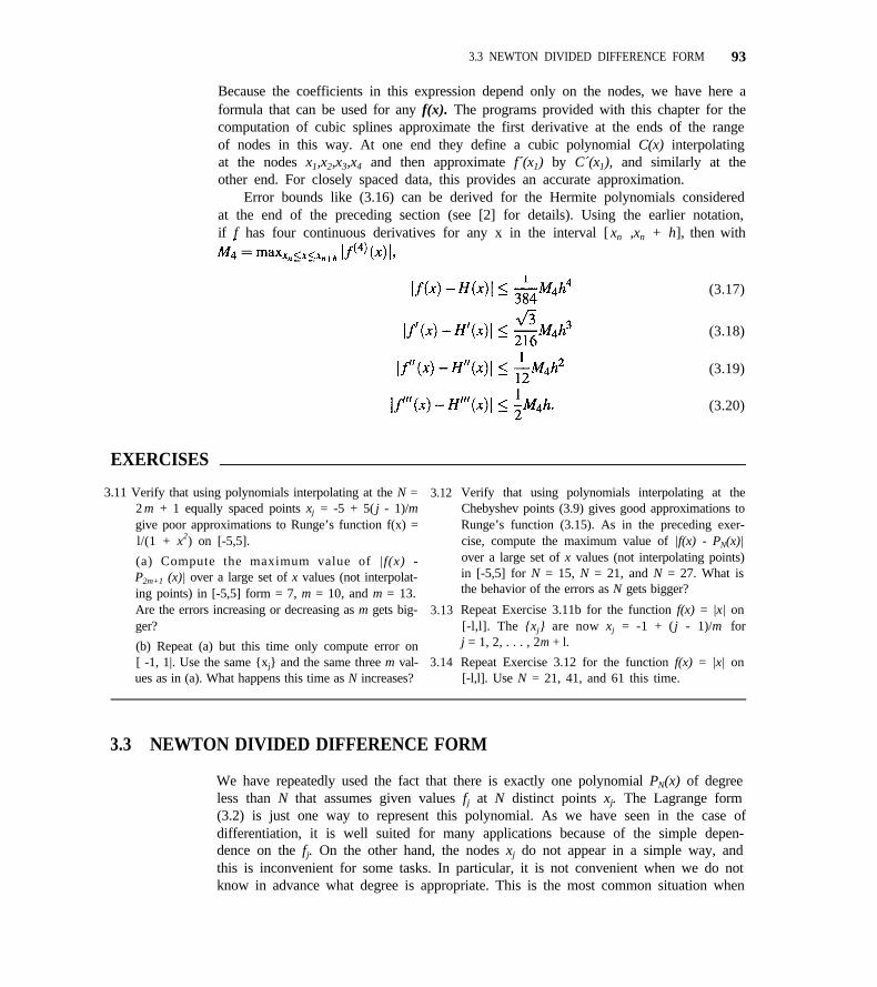
3.3 NEWTON DIVIDED DIFFERENCE FORM 93
Because the coefficients in this expression depend only on the nodes, we have here aformula that can be used for any f(x). The programs provided with this chapter for thecomputation of cubic splines approximate the first derivative at the ends of the rangeof nodes in this way. At one end they define a cubic polynomial C(x) interpolatingat the nodes x1,x2,x3,x4 and then approximate f´(x1) by C´(x1), and similarly at theother end. For closely spaced data, this provides an accurate approximation.
Error bounds like (3.16) can be derived for the Hermite polynomials consideredat the end of the preceding section (see [2] for details). Using the earlier notation,if f has four continuous derivatives for any x in the interval [ xn ,xn + h], then with
(3.17)
(3.18)
(3.19)
(3.20)
EXERCISES
3.11 Verify that using polynomials interpolating at the N = 3.122 m + 1 equally spaced points xj = -5 + 5( j - 1)/mgive poor approximations to Runge’s function f(x) =l/(1 + x2) on [-5,5].
(a) Compute the maximum value of |f(x) -P2m+1 (x)| over a large set of x values (not interpolat-ing points) in [-5,5] form = 7, m = 10, and m = 13.Are the errors increasing or decreasing as m gets big- 3.13ger?
(b) Repeat (a) but this time only compute error on[ -1, 1|. Use the same {xj} and the same three m val- 3.14ues as in (a). What happens this time as N increases?
Verify that using polynomials interpolating at theChebyshev points (3.9) gives good approximations toRunge’s function (3.15). As in the preceding exer-cise, compute the maximum value of |f(x) - PN(x)|over a large set of x values (not interpolating points)in [-5,5] for N = 15, N = 21, and N = 27. What isthe behavior of the errors as N gets bigger?
Repeat Exercise 3.11b for the function f(x) = |x| on[-l,l]. The {xj} are now xj = -1 + (j - 1)/m forj = 1, 2, . . . , 2m + l.
Repeat Exercise 3.12 for the function f(x) = |x| on[-l,l]. Use N = 21, 41, and 61 this time.
3.3 NEWTON DIVIDED DIFFERENCE FORM
We have repeatedly used the fact that there is exactly one polynomial PN(x) of degreeless than N that assumes given values fj at N distinct points xj. The Lagrange form(3.2) is just one way to represent this polynomial. As we have seen in the case ofdifferentiation, it is well suited for many applications because of the simple depen-dence on the fj. On the other hand, the nodes xj do not appear in a simple way, andthis is inconvenient for some tasks. In particular, it is not convenient when we do notknow in advance what degree is appropriate. This is the most common situation when
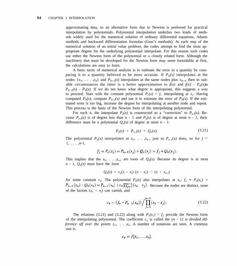
94 CHAPTER 3 INTERPOLATION
approximating data, so an alternative form due to Newton is preferred for practicalinterpolation by polynomials. Polynomial interpolation underlies two kinds of meth-ods widely used for the numerical solution of ordinary differential equations, Adamsmethods and backward differentiation formulas (Gear’s methods). At each step of thenumerical solution of an initial value problem, the codes attempt to find the most ap-propriate degree for the underlying polynomial interpolant. For this reason such codesuse either the Newton form of the polynomial or a closely related form. Although themachinery that must be developed for the Newton form may seem formidable at first,the calculations are easy to learn.
A basic tactic of numerical analysis is to estimate the error in a quantity by com-paring it to a quantity believed to be more accurate. If PN(x) interpolates at thenodes {x1, . . . ,xN} and PN+1(x) interpolates at the same nodes plus xN+l, then in suit-able circumstances the latter is a better approximation to f(x) and f(x) - PN(x) PN+1(x) - PN(x). If we do not know what degree is appropriate, this suggests a wayto proceed. Start with the constant polynomial P1(x) = f1 interpolating at x1. Havingcomputed PN(x), compute PN+l(x) and use it to estimate the error of PN(x). If the esti-mated error is too big, increase the degree by interpolating at another node and repeat.This process is the basis of the Newton form of the interpolating polynomial.
For each n, the interpolant Pn(x) is constructed as a “correction” to Pn-l(x). Be-cause Pn-l(x) is of degree less than n - 1 and Pn(x) is of degree at most n - 1, theirdifference must be a polynomial Qn(x) of degree at most n - 1:
Pn(x) = Pn-l(x) + Qn(x). (3.21)
The polynomial Pn(x) interpolates at xl,. . . ,xn-1 just as Pn-1(x) does, so for j =1, . . . ,n-1,
This implies that the xl,. . . ,xn-l are roots of Qn(x). Because its degree is at mostn - 1, Qn(x) must have the form
Qn(x) = cn(x - xl) (x - x2) ··· (x - xn-l)
for some constant cn. The polynomial Pn(x) also interpolates at xn: fn = Pn(xn) =
Because the nodes are distinct, noneof the factors (xn - xj) can vanish, and
(3.22)
The relations (3.21) and (3.22) along with P1(x1) = f1 provide the Newton formof the interpolating polynomial. The coefficient cn is called the (n - 1) st divided dif-ference off over the points x1,. . . ,xn. A number of notations are seen. A commonone is
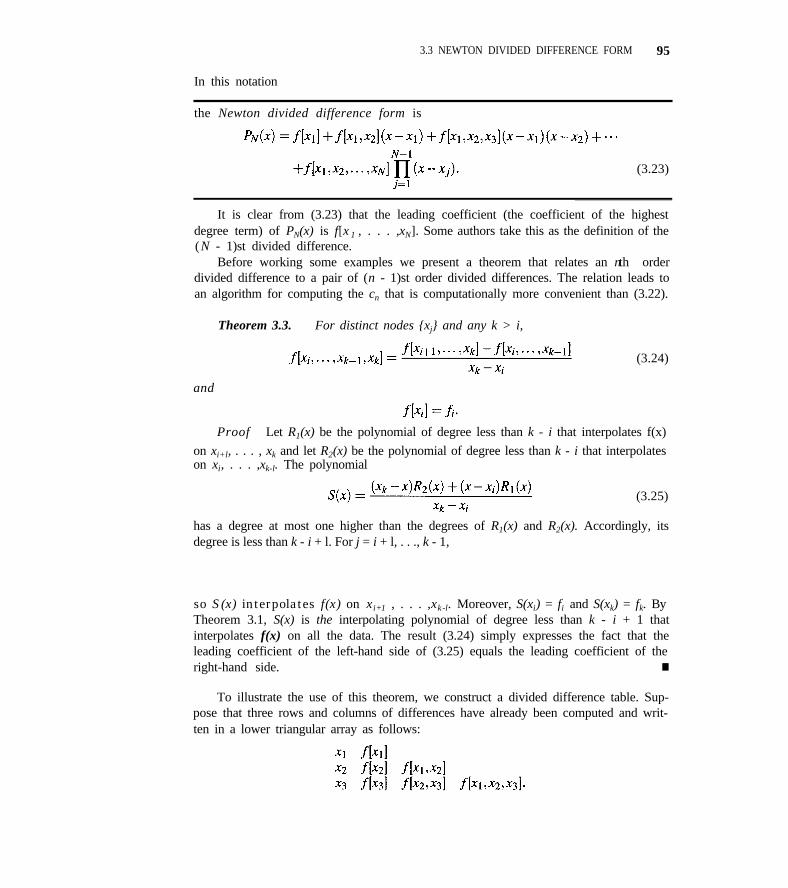
In this notation
3.3 NEWTON DIVIDED DIFFERENCE FORM 95
the Newton divided difference form is
(3.23)
It is clear from (3.23) that the leading coefficient (the coefficient of the highestdegree term) of PN(x) is f[x 1 , . . . ,xN]. Some authors take this as the definition of the(N - 1)st divided difference.
Before working some examples we present a theorem that relates an nth orderdivided difference to a pair of (n - 1)st order divided differences. The relation leads toan algorithm for computing the cn that is computationally more convenient than (3.22).
Theorem 3.3. For distinct nodes {xj} and any k > i,
(3.24)
and
Proof Let R1(x) be the polynomial of degree less than k - i that interpolates f(x)
on xi+l, . . . , xk and let R2(x) be the polynomial of degree less than k - i that interpolateson xi, . . . ,xk-l. The polynomial
(3.25)
has a degree at most one higher than the degrees of R1(x) and R2(x). Accordingly, itsdegree is less than k - i + l. For j = i + l, . . ., k - 1,
so S(x) interpolates f(x) on xi+1 , . . . ,xk-l. Moreover, S(xi) = fi and S(xk) = fk. ByTheorem 3.1, S(x) is the interpolating polynomial of degree less than k - i + 1 thatinterpolates f(x) on all the data. The result (3.24) simply expresses the fact that theleading coefficient of the left-hand side of (3.25) equals the leading coefficient of theright-hand side. n
To illustrate the use of this theorem, we construct a divided difference table. Sup-pose that three rows and columns of differences have already been computed and writ-ten in a lower triangular array as follows:
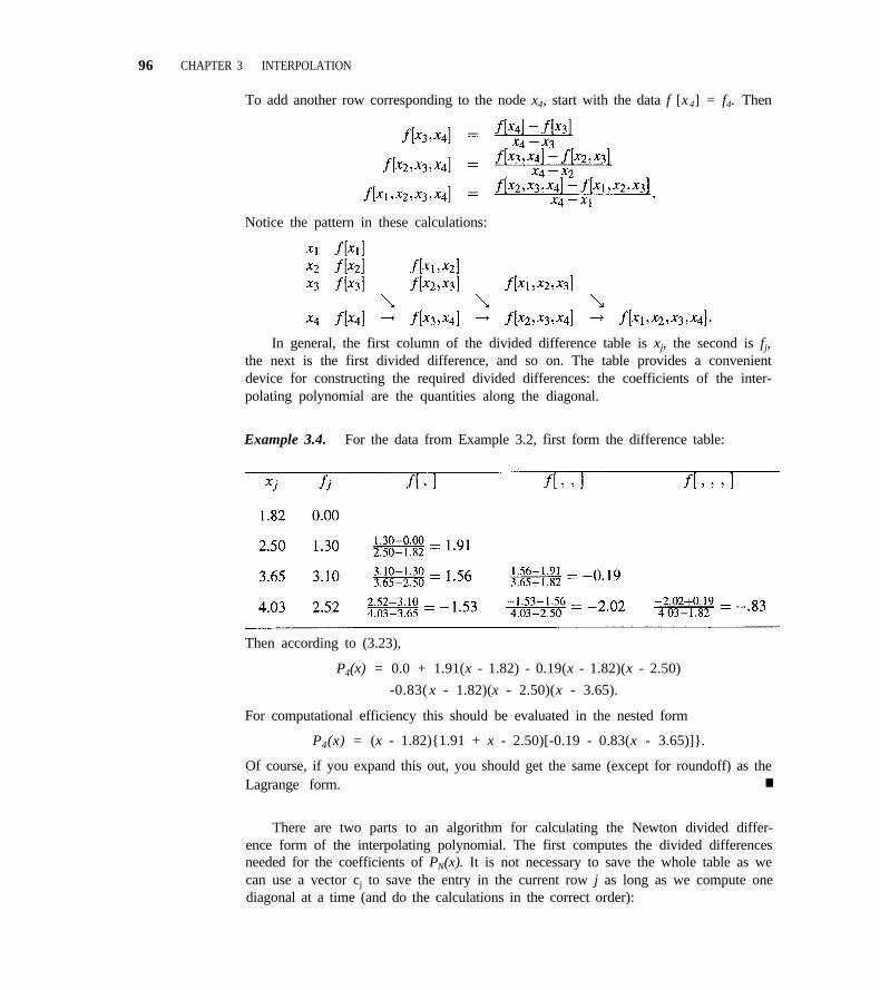
96 CHAPTER 3 INTERPOLATION
To add another row corresponding to the node x4, start with the data f [x4] = f4. Then
Notice the pattern in these calculations:
In general, the first column of the divided difference table is xj, the second is fj,the next is the first divided difference, and so on. The table provides a convenientdevice for constructing the required divided differences: the coefficients of the inter-polating polynomial are the quantities along the diagonal.
Example 3.4. For the data from Example 3.2, first form the difference table:
Then according to (3.23),
P4(x) = 0.0 + 1.91(x - 1.82) - 0.19(x - 1.82)(x - 2.50)
-0.83( x - 1.82)(x - 2.50)(x - 3.65).
For computational efficiency this should be evaluated in the nested form
P4(x) = (x - 1.82){1.91 + x - 2.50)[-0.19 - 0.83(x - 3.65)]}.
Of course, if you expand this out, you should get the same (except for roundoff) as theLagrange form. n
There are two parts to an algorithm for calculating the Newton divided differ-ence form of the interpolating polynomial. The first computes the divided differencesneeded for the coefficients of PN(x). It is not necessary to save the whole table as wecan use a vector cj to save the entry in the current row j as long as we compute onediagonal at a time (and do the calculations in the correct order):
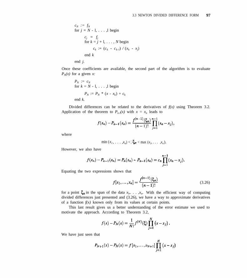
3.3 NEWTON DIVIDED DIFFERENCE FORM 97
cN := fN
for j = N - l, . . . ,l begin
cj = fj
for k = j + l, . . . , N begin
ck := (ck - ck-l) / (xk - xj)
end k
end j.
Once these coefficients are available, the second part of the algorithm is to evaluatePN(x) for a given x:
PN := cN
for k = N - l, . . . ,l begin
PN := PN * (x - xk) + ck
end k.
Divided differences can be related to the derivatives of f(x) using Theorem 3.2.Application of the theorem to Pn-l(x) with x = xn leads to
where
min (x1 , . . . ,xn) < < max (x1, . . . ,xn).
However, we also have
Equating the two expressions shows that
(3.26)
for a point in the span of the data xl,. . . ,xn. With the efficient way of computingdivided differences just presented and (3.26), we have a way to approximate derivativesof a function f(x) known only from its values at certain points.
This last result gives us a better understanding of the error estimate we used tomotivate the approach. According to Theorem 3.2,
We have just seen that
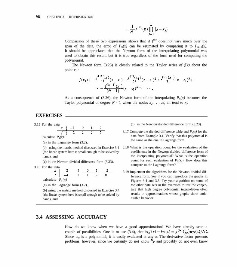
98 CHAPTER 3 INTERPOLATION
Comparison of these two expressions shows that if f(N) does not vary much over thespan of the data, the error of PN(x) can be estimated by comparing it to PN+1(x).It should be appreciated that the Newton form of the interpolating polynomial wasused to obtain this result, but it is true regardless of the form used for computing thepolynomial.
The Newton form (3.23) is closely related to the Taylor series of f(x) about thepoint xl :
As a consequence of (3.26), the Newton form of the interpolating PN(x) becomes theTaylor polynomial of degree N - 1 when the nodes x2,. . . ,xn all tend to xl.
EXERCISES
3.15 For the data (c) in the Newton divided difference form (3.23).
3.17 Compute the divided difference table and P3(x) for the
calculate P4(x) data from Example 3.1. Verify that this polynomial is
(a) in the Lagrange form (3.2),the same as the one in Lagrange form.
(b) using the matrix method discussed in Exercise 3.4(the linear system here is small enough to be solved byhand), and
(c) in the Newton divided difference form (3.23).
3.16 For the data
calculate P5(x)
(a) in the Lagrange form (3.2),
(b) using the matrix method discussed in Exercise 3.4(the linear system here is small enough to be solved byhand), and
3.18 What is the operation count for the evaluation of thecoefficients in the Newton divided difference form ofthe interpolating polynomial? What is the operationcount for each evaluation of PN(x)? How does thiscompare to the Lagrange form?
3.19 Implement the algorithms for the Newton divided dif-ference form. See if you can reproduce the graphs inFigures 3.4 and 3.5. Try your algorithm on some ofthe other data sets in the exercises to test the conjec-ture that high degree polynomial interpolation oftenresults in approximations whose graphs show unde-sirable behavior.
3.4 ASSESSING ACCURACY
How do we know when we have a good approximation? We have already seen acouple of possibilities. One is to use (3.4), that is,Since wN is a polynomial, it is easily evaluated at any x. The derivative factor presentsproblems, however, since we certainly do not know and probably do not even know
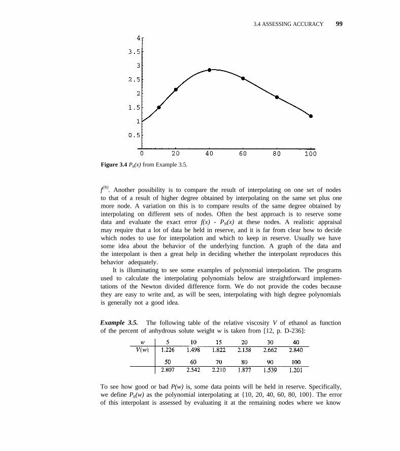
3.4 ASSESSING ACCURACY 99
Figure 3.4 P6(x) from Example 3.5.
f(N). Another possibility is to compare the result of interpolating on one set of nodesto that of a result of higher degree obtained by interpolating on the same set plus onemore node. A variation on this is to compare results of the same degree obtained byinterpolating on different sets of nodes. Often the best approach is to reserve somedata and evaluate the exact error f(x) - PN(x) at these nodes. A realistic appraisalmay require that a lot of data be held in reserve, and it is far from clear how to decidewhich nodes to use for interpolation and which to keep in reserve. Usually we havesome idea about the behavior of the underlying function. A graph of the data andthe interpolant is then a great help in deciding whether the interpolant reproduces thisbehavior adequately.
It is illuminating to see some examples of polynomial interpolation. The programsused to calculate the interpolating polynomials below are straightforward implemen-tations of the Newton divided difference form. We do not provide the codes becausethey are easy to write and, as will be seen, interpolating with high degree polynomialsis generally not a good idea.
Example 3.5. The following table of the relative viscosity V of ethanol as functionof the percent of anhydrous solute weight w is taken from [12, p. D-236]:
To see how good or bad P(w) is, some data points will be held in reserve. Specifically,we define P6(w) as the polynomial interpolating at {10, 20, 40, 60, 80, 100}. The errorof this interpolant is assessed by evaluating it at the remaining nodes where we know
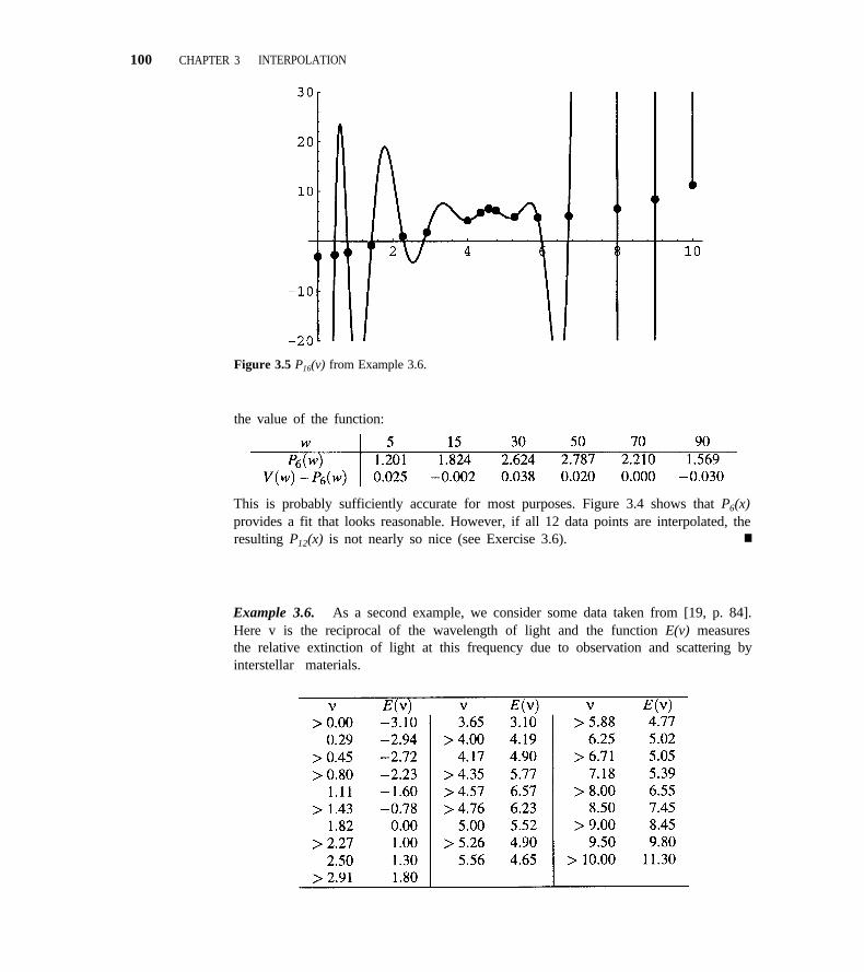
100 CHAPTER 3 INTERPOLATION
Figure 3.5 P16(v) from Example 3.6.
the value of the function:
This is probably sufficiently accurate for most purposes. Figure 3.4 shows that P6(x)provides a fit that looks reasonable. However, if all 12 data points are interpolated, theresulting P12(x) is not nearly so nice (see Exercise 3.6). n
Example 3.6. As a second example, we consider some data taken from [19, p. 84].Here v is the reciprocal of the wavelength of light and the function E(v) measuresthe relative extinction of light at this frequency due to observation and scattering byinterstellar materials.
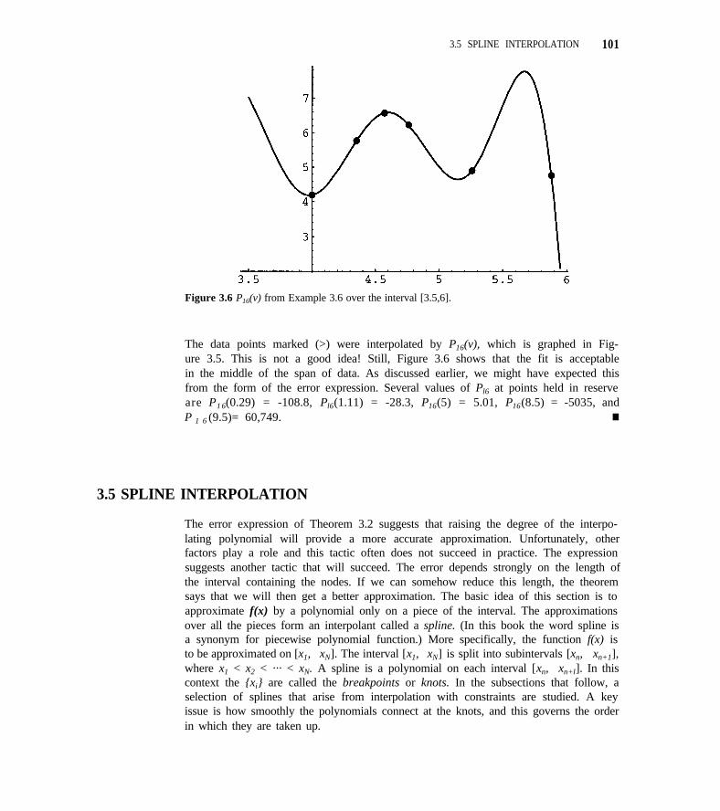
3.5 SPLINE INTERPOLATION 101
Figure 3.6 P16(v) from Example 3.6 over the interval [3.5,6].
The data points marked (>) were interpolated by P16(v), which is graphed in Fig-ure 3.5. This is not a good idea! Still, Figure 3.6 shows that the fit is acceptablein the middle of the span of data. As discussed earlier, we might have expected thisfrom the form of the error expression. Several values of Pl6 at points held in reserveare P1 6(0.29) = -108.8, Pl6(1.11) = -28.3, P16(5) = 5.01, P16(8.5) = -5035, andP 1 6 (9.5)= 60,749. n
3.5 SPLINE INTERPOLATION
The error expression of Theorem 3.2 suggests that raising the degree of the interpo-lating polynomial will provide a more accurate approximation. Unfortunately, otherfactors play a role and this tactic often does not succeed in practice. The expressionsuggests another tactic that will succeed. The error depends strongly on the length ofthe interval containing the nodes. If we can somehow reduce this length, the theoremsays that we will then get a better approximation. The basic idea of this section is toapproximate f(x) by a polynomial only on a piece of the interval. The approximationsover all the pieces form an interpolant called a spline. (In this book the word spline isa synonym for piecewise polynomial function.) More specifically, the function f(x) isto be approximated on [x1, xN]. The interval [x1, xN] is split into subintervals [xn, xn+1],where x1 < x2 < ··· < xN. A spline is a polynomial on each interval [xn, xn+l]. In thiscontext the {xi} are called the breakpoints or knots. In the subsections that follow, aselection of splines that arise from interpolation with constraints are studied. A keyissue is how smoothly the polynomials connect at the knots, and this governs the orderin which they are taken up.
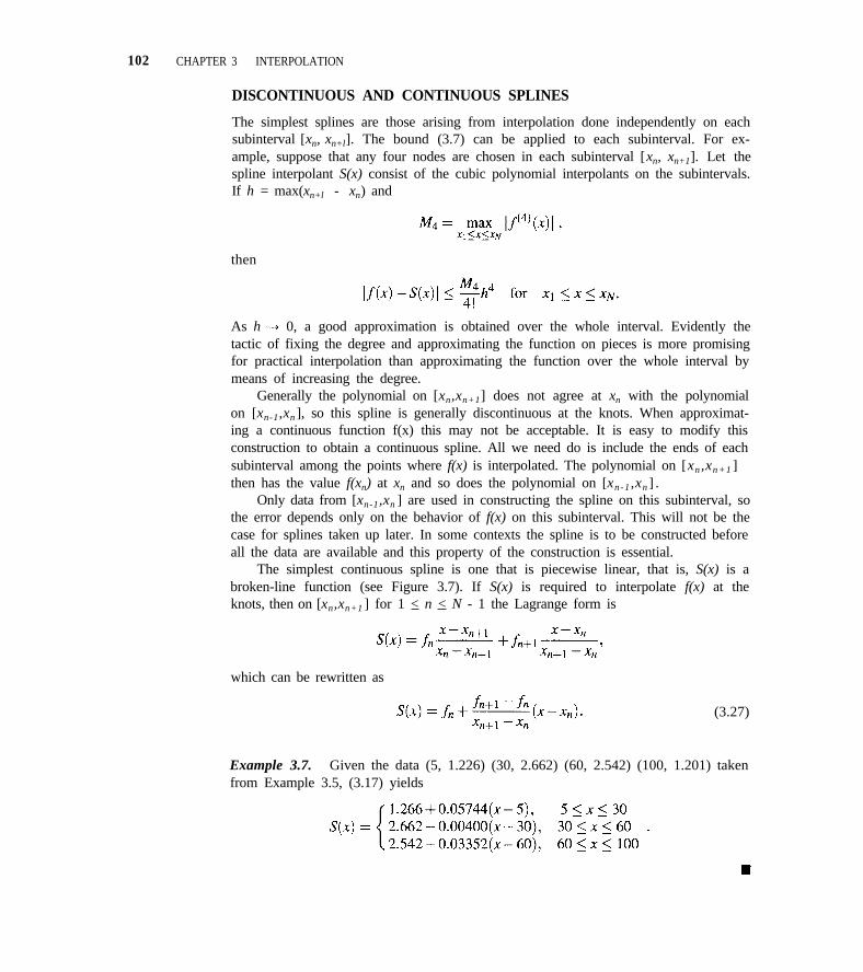
102 CHAPTER 3 INTERPOLATION
DISCONTINUOUS AND CONTINUOUS SPLINES
The simplest splines are those arising from interpolation done independently on eachsubinterval [xn, xn+l]. The bound (3.7) can be applied to each subinterval. For ex-ample, suppose that any four nodes are chosen in each subinterval [xn, xn+1]. Let thespline interpolant S(x) consist of the cubic polynomial interpolants on the subintervals.If h = max(xn+l - xn) and
then
As h 0, a good approximation is obtained over the whole interval. Evidently thetactic of fixing the degree and approximating the function on pieces is more promisingfor practical interpolation than approximating the function over the whole interval bymeans of increasing the degree.
Generally the polynomial on [xn,xn+1] does not agree at xn with the polynomialon [xn-1,xn ], so this spline is generally discontinuous at the knots. When approximat-ing a continuous function f(x) this may not be acceptable. It is easy to modify thisconstruction to obtain a continuous spline. All we need do is include the ends of eachsubinterval among the points where f(x) is interpolated. The polynomial on [xn ,xn+1 ] then has the value f(xn) at xn and so does the polynomial on [xn-1 ,xn ] .
Only data from [xn-1,xn ] are used in constructing the spline on this subinterval, sothe error depends only on the behavior of f(x) on this subinterval. This will not be thecase for splines taken up later. In some contexts the spline is to be constructed beforeall the data are available and this property of the construction is essential.
The simplest continuous spline is one that is piecewise linear, that is, S(x) is abroken-line function (see Figure 3.7). If S(x) is required to interpolate f(x) at theknots, then on [xn,xn+1 ] for 1 < n < N - 1 the Lagrange form is
which can be rewritten as
(3.27)
Example 3.7. Given the data (5, 1.226) (30, 2.662) (60, 2.542) (100, 1.201) takenfrom Example 3.5, (3.17) yields
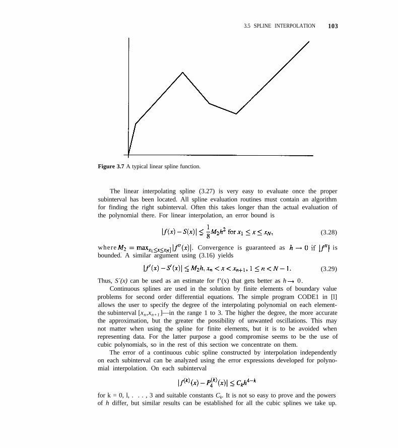
3.5 SPLINE INTERPOLATION 103
Figure 3.7 A typical linear spline function.
The linear interpolating spline (3.27) is very easy to evaluate once the propersubinterval has been located. All spline evaluation routines must contain an algorithmfor finding the right subinterval. Often this takes longer than the actual evaluation ofthe polynomial there. For linear interpolation, an error bound is
(3.28)
where Convergence is guaranteed as isbounded. A similar argument using (3.16) yields
(3.29)
Thus, S´(x) can be used as an estimate for f’(x) that gets better as h 0.Continuous splines are used in the solution by finite elements of boundary value
problems for second order differential equations. The simple program CODE1 in [l]allows the user to specify the degree of the interpolating polynomial on each element-the subinterval [xn,xn+1 ]—in the range 1 to 3. The higher the degree, the more accuratethe approximation, but the greater the possibility of unwanted oscillations. This maynot matter when using the spline for finite elements, but it is to be avoided whenrepresenting data. For the latter purpose a good compromise seems to be the use ofcubic polynomials, so in the rest of this section we concentrate on them.
The error of a continuous cubic spline constructed by interpolation independentlyon each subinterval can be analyzed using the error expressions developed for polyno-mial interpolation. On each subinterval
for k = 0, l, . . . , 3 and suitable constants Ck. It is not so easy to prove and the powersof h differ, but similar results can be established for all the cubic splines we take up.
104 CHAPTER 3 INTERPOLATION
The point, though, is that on each subinterval This implies that for suf-ficiently small h, P´4(x) has the same sign as f´(x) as long as f´(x) 0. Put differently,except near the extrema of f(x), for small h the spline is monotonely increasing (de-creasing) wherever f(x) is. The same argument applies to the second derivative andleads to the conclusion that except near inflection points of f(x), for small h the splineis concave (convex) wherever f(x) is. We conclude that for small h, the spline will re-produce the shape of the function it interpolates. The same will be true of all the cubicsplines we take up. This is one reason why spline interpolation is much more satis-factory than interpolation by high degree polynomials. But what if h is not “small”?When the data are sparse, it is necessary to impose conditions on the spline to preservethe shape of the function, one of the matters we take up in the next subsection.
CONTINUOUS FIRST DERIVATIVE
If we have derivative data available, it is easy to extend the approach of the precedingsubsection to obtain an interpolant with a continuous derivative. For example, wecould interpolate f(xn), f´(x,), f(xn+1), f´(xn+1) by the cubic Hermite interpolatingpolynomial on [xn,xn+1 ]. Doing this on each subinterval produces a spline H(x) witha continuous first derivative. Each interval is treated independently, so the bounds(3.17)-(3.20) hold and show that a good approximation is obtained. In the chapter ondifferential equations, we produce, for successive n, approximations to a function y(x)and its derivative at the points xn, xn + h/2, and xn + h. By forming the quintic (degree5) Hermite interpolant to these data, a spline with a continuous derivative is formedthat approximates y(x) and y´(x) for all x. It is especially important in this context thatthe interval [xn,xn + h] is handled independently because generally it is only the dataon this interval that are available when interpolation is done.
Let us now consider the representation of data when only f(xi) values are knownand there are not many of them. It has been found that a cubic spline H(x) yields a plotpleasing to the eye if it has a continuous derivative and if it preserves monotonicity. Bythe latter is meant that if fn < fn+1, then H(x) increases on (xn,xn+1 ) and if fn > fn+1,then H(x) decreases. The point is to avoid oscillations that do not appear in the data.A moment’s thought shows that linear splines preserve monotonicity. The problemwith them is that their graphs have “corners.” By going to cubits and a continuousfirst derivative, we avoid the corners. Such a “shape-preserving” interpolant can beconstructed along the lines of the cubic Hermite interpolant. The cubits on [xn - 1 ,xn]and [xn,xn+l] both interpolate to fn at xn. If the first derivative is to be continuous, thefirst derivatives of the two cubits must have the same value at xn, but now the value ofthis derivative is an unknown parameter that we choose to achieve monotonicity.
As in (3.11) the cubic is written in the form
for xn < x < xn+1, 1 < n < N - 1. Note that the parameter bn is just the slope ofH(x) at the point xn. Proceeding as in the derivation of (3.12)–(3.14) with the notationhn = xn+l - xn and = (fn+ 1 - fn) /hn yields
an = fn
3.5 SPLINE INTERPOLATION 105
(3.30)
These equations result from solving the three interpolation conditions H(xn) = fn,H(xn+l) = fn+1, and H´(xn+l) = bn+l for the three unknowns an, cn, and dn.
The quantity A, is the slope of the line through (x n , f n ) and (xn+1, fn+1). If = 0,it seems reasonable to force H(x) to be constant on [xn ,xn + 1], that is, to make the slopesbn = bn+1 = 0. If 0, let us define αn = bn/ and βn = bn+1 To preservemonotonicity it is necessary that the sign of the slope of H(x) at xn and xn+l be thesame as that of Mathematically this is αn > 0, βn > 0.
A sufficient condition on α and β to preserve monotonicity was found by Fergusonand Miller [7]. This was independently discovered by Fritsch and Carlson and pub-lished in the more accessible reference [10]. The argument involves studying H’(x)as a function of αn and βn. This is not too complicated since H’(x) is a quadratic on(xn ,xn+l ). A simple condition that guarantees monotonicity is preserved is that αn
and βn lie in the interval [0,3]. There are many formulas for α n and βn that satisfy thisrestriction. One given in [9] that works pretty well is to use
with
(3.3 1)
(3.32)
for n = 2, 3, . . . , N - 1. If then the slopes change sign at xn. In sucha case we probably should not impose any requirements on the slope of H(x) at xn.Some people suggest setting bn = 0 when this happens. Others say to go ahead anduse (3.31) as long as there is no division by zero. The heuristic actually chosen canhave a significant impact on the behavior of the shape-preserving cubic spline nearthose regions where At the ends the simplest rule is to use b1 = andbN = A better choice is to use the end slope of the quadratic interpolatingthe three closest data points (assuming it satisfies the constraint on a and β); otherpossibilities are given in [9]. With (3.31) and the simple choice for b1 and bN it is easyto show that the sufficient conditions on αn and βn are satisfied. At the ends α1 = 1and βN-1 = l, which are certainly in [0,3]. For n = 2, 3, . . . , N - 1,so αn = and
as desired.The algorithm for H(x) is very simple. Compute b1 by whatever formula you
choose; for n = 2, 3, . . . , N - 1 take bn = 0 if otherwise compute bn from(3.31), (3.32). Compute bN. The values cn and dn can be computed from (3.30) forn = l, . . . , N - 1 either at the same time the bn are computed or in a separate passover the data. Later in this chapter we provide a routine SVALUE/Spline_value for theevaluation of H(x).
Examination of the algorithm shows that on the subinterval [xn ,xn + 1 ], the splinedepends on the data (xn-1, fn-1) , (xn, fn) (xn+l, fn+l) and (xn+2, fn+2). It shouldbe no surprise that it depends on data from adjacent subintervals because the first
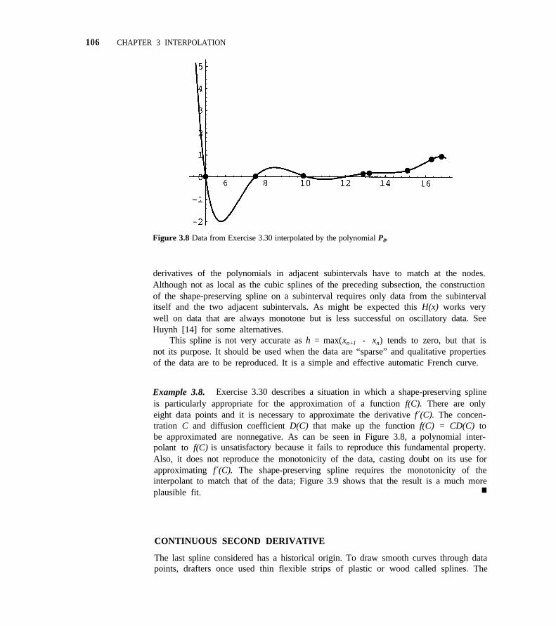
106 CHAPTER 3 INTERPOLATION
Figure 3.8 Data from Exercise 3.30 interpolated by the polynomial P8.
derivatives of the polynomials in adjacent subintervals have to match at the nodes.Although not as local as the cubic splines of the preceding subsection, the constructionof the shape-preserving spline on a subinterval requires only data from the subintervalitself and the two adjacent subintervals. As might be expected this H(x) works verywell on data that are always monotone but is less successful on oscillatory data. SeeHuynh [14] for some alternatives.
This spline is not very accurate as h = max(xn+l - xn) tends to zero, but that isnot its purpose. It should be used when the data are “sparse” and qualitative propertiesof the data are to be reproduced. It is a simple and effective automatic French curve.
Example 3.8. Exercise 3.30 describes a situation in which a shape-preserving splineis particularly appropriate for the approximation of a function f(C). There are onlyeight data points and it is necessary to approximate the derivative f´(C). The concen-tration C and diffusion coefficient D(C) that make up the function f(C) = CD(C) tobe approximated are nonnegative. As can be seen in Figure 3.8, a polynomial inter-polant to f(C) is unsatisfactory because it fails to reproduce this fundamental property.Also, it does not reproduce the monotonicity of the data, casting doubt on its use forapproximating f´(C). The shape-preserving spline requires the monotonicity of theinterpolant to match that of the data; Figure 3.9 shows that the result is a much moreplausible fit. n
CONTINUOUS SECOND DERIVATIVE
The last spline considered has a historical origin. To draw smooth curves through datapoints, drafters once used thin flexible strips of plastic or wood called splines. The
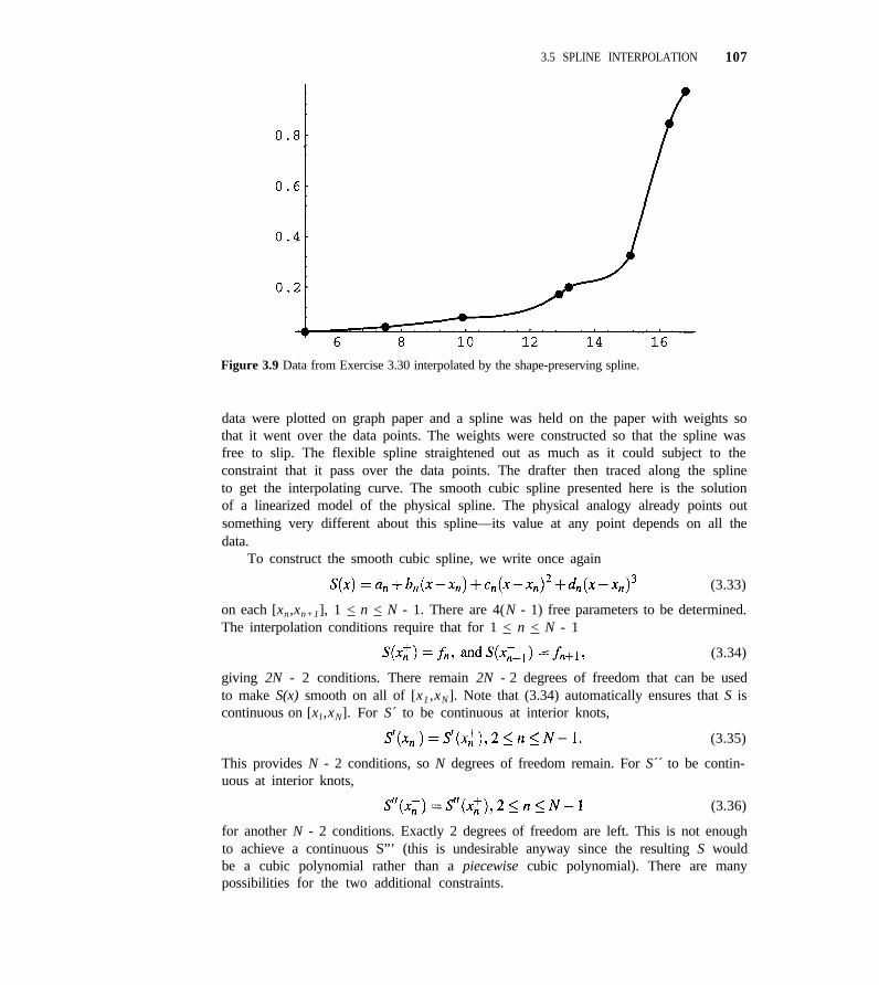
3.5 SPLINE INTERPOLATION 107
Figure 3.9 Data from Exercise 3.30 interpolated by the shape-preserving spline.
data were plotted on graph paper and a spline was held on the paper with weights sothat it went over the data points. The weights were constructed so that the spline wasfree to slip. The flexible spline straightened out as much as it could subject to theconstraint that it pass over the data points. The drafter then traced along the splineto get the interpolating curve. The smooth cubic spline presented here is the solutionof a linearized model of the physical spline. The physical analogy already points outsomething very different about this spline—its value at any point depends on all thedata.
To construct the smooth cubic spline, we write once again
(3.33)
on each [xn,xn+1], 1 < n < N - 1. There are 4(N - 1) free parameters to be determined.The interpolation conditions require that for 1 < n < N - 1
(3.34)
giving 2N - 2 conditions. There remain 2N - 2 degrees of freedom that can be usedto make S(x) smooth on all of [x1 ,xN]. Note that (3.34) automatically ensures that S iscontinuous on [x l ,xN]. For S´ to be continuous at interior knots,
(3.35)
This provides N - 2 conditions, so N degrees of freedom remain. For S´´ to be contin-uous at interior knots,
(3.36)
for another N - 2 conditions. Exactly 2 degrees of freedom are left. This is not enoughto achieve a continuous S”’ (this is undesirable anyway since the resulting S wouldbe a cubic polynomial rather than a piecewise cubic polynomial). There are manypossibilities for the two additional constraints.
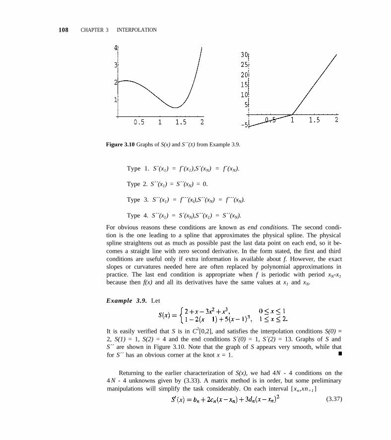
108 CHAPTER 3 INTERPOLATION
Figure 3.10 Graphs of S(x) and S´´(X) from Example 3.9.
Type 1. S´(x1) = f´(x1),S´(xN) = f´(xN).
Type 2. S´´(x1) = S´´(xN) = 0.
Type 3. S´´(x1) = f´´´(xl),S´´(xN) = f´´´(xN).
Type 4. S´´(x1) = S´(xN),S´´(x1) = S´´(xN).
For obvious reasons these conditions are known as end conditions. The second condi-tion is the one leading to a spline that approximates the physical spline. The physicalspline straightens out as much as possible past the last data point on each end, so it be-comes a straight line with zero second derivative. In the form stated, the first and thirdconditions are useful only if extra information is available about f. However, the exactslopes or curvatures needed here are often replaced by polynomial approximations inpractice. The last end condition is appropriate when f is periodic with period xN-x1
because then f(x) and all its derivatives have the same values at x1 and xN.
Example 3.9. Let
It is easily verified that S is in C2[0,2], and satisfies the interpolation conditions S(0) =2, S(1) = 1, S(2) = 4 and the end conditions S´(0) = 1, S´(2) = 13. Graphs of S andS´´ are shown in Figure 3.10. Note that the graph of S appears very smooth, while thatfor S´´ has an obvious corner at the knot x = 1. n
Returning to the earlier characterization of S(x), we had 4N - 4 conditions on the4 N - 4 unknowns given by (3.33). A matrix method is in order, but some preliminarymanipulations will simplify the task considerably. On each interval [xn,xn+1 ]
(3.37)
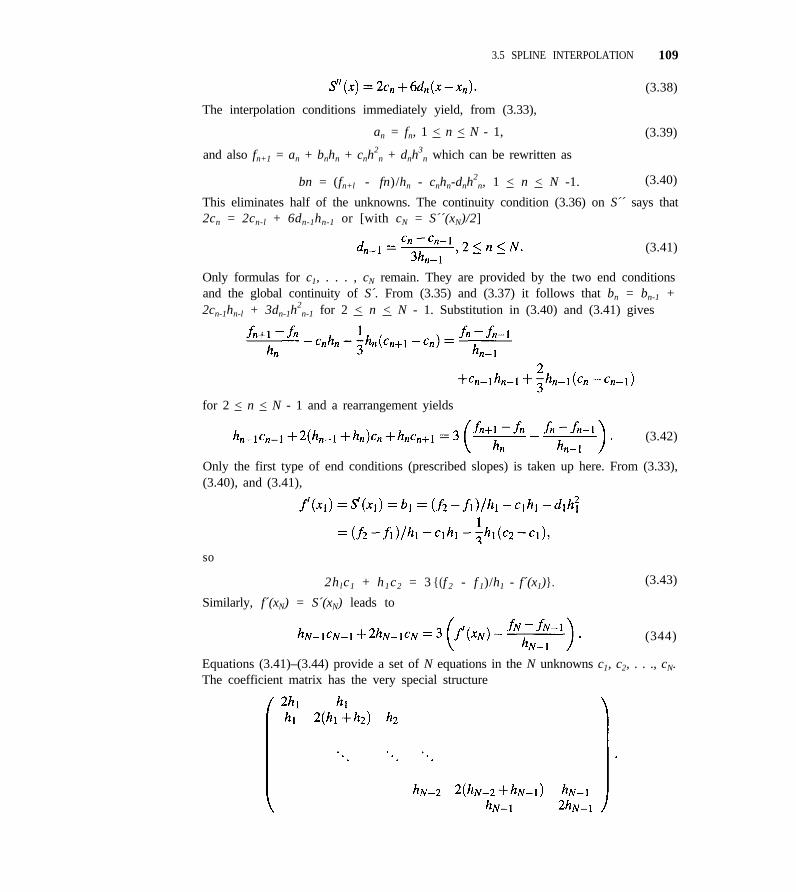
3.5 SPLINE INTERPOLATION 109
(3.38)
The interpolation conditions immediately yield, from (3.33),
an = fn, 1 < n < N - 1, (3.39)
and also fn+1 = an + bnhn + cnh2
n + dnh3
n which can be rewritten as
bn = (fn+l - fn)/hn - cnhn-dnh2
n, 1 < n < N -1. (3.40)
This eliminates half of the unknowns. The continuity condition (3.36) on S´´ says that2cn = 2cn-l + 6dn-1hn-1 or [with cN = S´´(xN)/2]
(3.41)
Only formulas for c1, . . . , cN remain. They are provided by the two end conditionsand the global continuity of S´. From (3.35) and (3.37) it follows that bn = bn-1 +2cn-1hn-l + 3dn-1h
2n-1 for 2 < n < N - 1. Substitution in (3.40) and (3.41) gives
for 2 < n < N - 1 and a rearrangement yields
(3.42)
Only the first type of end conditions (prescribed slopes) is taken up here. From (3.33),(3.40), and (3.41),
so
2h lc1 + h1c2 = 3 {(f 2 - f 1)/h1 - f´(x1)}.
Similarly, f´(xN) = S´(xN) leads to
(3.43)
(344)
Equations (3.41)–(3.44) provide a set of N equations in the N unknowns c1, c2, . . ., cN.The coefficient matrix has the very special structure
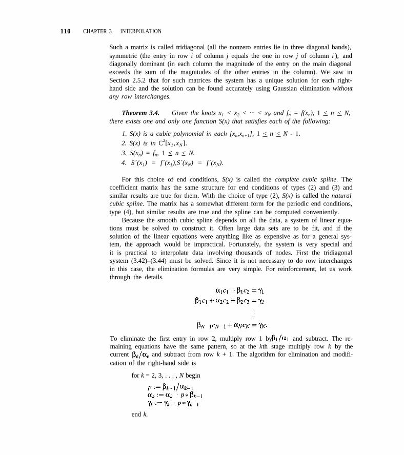
110 CHAPTER 3 INTERPOLATION
Such a matrix is called tridiagonal (all the nonzero entries lie in three diagonal bands),symmetric (the entry in row i of column j equals the one in row j of column i ), anddiagonally dominant (in each column the magnitude of the entry on the main diagonalexceeds the sum of the magnitudes of the other entries in the column). We saw inSection 2.5.2 that for such matrices the system has a unique solution for each right-hand side and the solution can be found accurately using Gaussian elimination withoutany row interchanges.
Theorem 3.4. Given the knots x1 < x2 < ··· < xN and fn = f(xn), 1 < n < N,there exists one and only one function S(x) that satisfies each of the following:
1. S(x) is a cubic polynomial in each [xn,xn+1], 1 < n < N - 1.
2. S(x) is in C2[x1 ,xN].
3. S(xn) = fn, 1 < n < N.
4. S´(x1) = f´(x1),S´(xN) = f´(xN).
For this choice of end conditions, S(x) is called the complete cubic spline. Thecoefficient matrix has the same structure for end conditions of types (2) and (3) andsimilar results are true for them. With the choice of type (2), S(x) is called the naturalcubic spline. The matrix has a somewhat different form for the periodic end conditions,type (4), but similar results are true and the spline can be computed conveniently.
Because the smooth cubic spline depends on all the data, a system of linear equa-tions must be solved to construct it. Often large data sets are to be fit, and if thesolution of the linear equations were anything like as expensive as for a general sys-tem, the approach would be impractical. Fortunately, the system is very special andit is practical to interpolate data involving thousands of nodes. First the tridiagonalsystem (3.42)–(3.44) must be solved. Since it is not necessary to do row interchangesin this case, the elimination formulas are very simple. For reinforcement, let us workthrough the details.
To eliminate the first entry in row 2, multiply row 1 by and subtract. The re-maining equations have the same pattern, so at the kth stage multiply row k by thecurrent and subtract from row k + 1. The algorithm for elimination and modifi-cation of the right-hand side is
for k = 2, 3, . . . , N begin
end k.
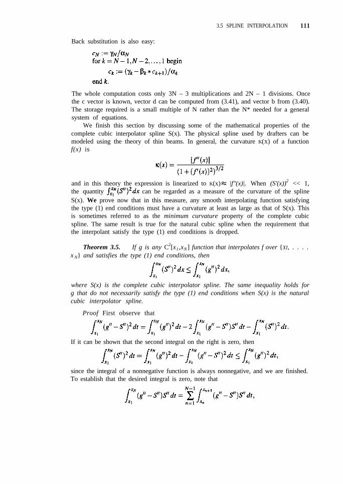
3.5 SPLINE INTERPOLATION 111
Back substitution is also easy:
The whole computation costs only 3N – 3 multiplications and 2N – 1 divisions. Oncethe c vector is known, vector d can be computed from (3.41), and vector b from (3.40).The storage required is a small multiple of N rather than the N* needed for a generalsystem of equations.
We finish this section by discussing some of the mathematical properties of thecomplete cubic interpolator spline S(x). The physical spline used by drafters can bemodeled using the theory of thin beams. In general, the curvature K(X) of a functionf(x) is
and in this theory the expression is linearized to K(x) |f"(x)|. When (S'(x))2 << 1,the quantity can be regarded as a measure of the curvature of the splineS(x). We prove now that in this measure, any smooth interpolating function satisfyingthe type (1) end conditions must have a curvature at least as large as that of S(x). Thisis sometimes referred to as the minimum curvature property of the complete cubicspline. The same result is true for the natural cubic spline when the requirement thatthe interpolant satisfy the type (1) end conditions is dropped.
Theorem 3.5. If g is any C2[x1,xN] function that interpolates f over {XI, . . . .x N} and satisfies the type (1) end conditions, then
where S(x) is the complete cubic interpolator spline. The same inequality holds forg that do not necessarily satisfy the type (1) end conditions when S(x) is the naturalcubic interpolator spline.
Proof First observe that
If it can be shown that the second integral on the right is zero, then
since the integral of a nonnegative function is always nonnegative, and we are finished.To establish that the desired integral is zero, note that
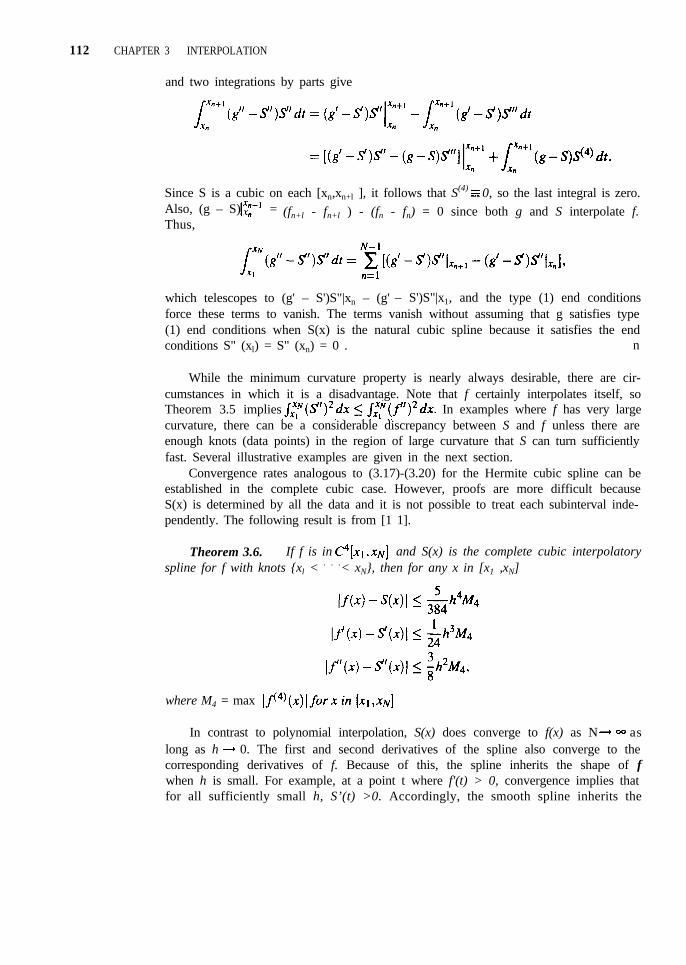
112 CHAPTER 3 INTERPOLATION
and two integrations by parts give
Since S is a cubic on each [xn,xn+l ], it follows that S(4) 0, so the last integral is zero.Also, (g – S) = (fn+l - fn+l ) - (fn - fn) = 0 since both g and S interpolate f.Thus,
which telescopes to (g' – S')S"|xn – (g' – S')S"|x1, and the type (1) end conditionsforce these terms to vanish. The terms vanish without assuming that g satisfies type(1) end conditions when S(x) is the natural cubic spline because it satisfies the endconditions S" (xl) = S" (xn) = 0 . n
While the minimum curvature property is nearly always desirable, there are cir-cumstances in which it is a disadvantage. Note that f certainly interpolates itself, soTheorem 3.5 implies In examples where f has very largecurvature, there can be a considerable discrepancy between S and f unless there areenough knots (data points) in the region of large curvature that S can turn sufficientlyfast. Several illustrative examples are given in the next section.
Convergence rates analogous to (3.17)-(3.20) for the Hermite cubic spline can beestablished in the complete cubic case. However, proofs are more difficult becauseS(x) is determined by all the data and it is not possible to treat each subinterval inde-pendently. The following result is from [1 1].
Theorem 3.6. If f is in and S(x) is the complete cubic interpolatoryspline for f with knots {xl < . . .< xN}, then for any x in [x1 ,xN]
where M4 = max
In contrast to polynomial interpolation, S(x) does converge to f(x) as N aslong as h 0. The first and second derivatives of the spline also converge to thecorresponding derivatives of f. Because of this, the spline inherits the shape of fwhen h is small. For example, at a point t where f'(t) > 0, convergence implies thatfor all sufficiently small h, S’(t) >0. Accordingly, the smooth spline inherits the
3.5 SPLINE INTERPOLATION 113
monotonicity of f for small h, except possibly near the extrema of f. The shape-preserving spline is required only when the data are so sparse that we must imposedirectly the property of monotonicity on the spline. The same argument shows that forsmall h, the smooth spline is convex where f is, except possibly near inflection points.
The complete cubic spline will converge when f has fewer than four continuousderivatives on [a,b], just not as fast. Experimentation with a physical spline showsthat the farther a node xk is from a given point t, the less the effect of the value of fk
on S(t). This is also true of the mathematical spline, and a careful analysis, see [16],of convergence reveals that the rate of convergence at t depends only on how smoothf(x) is near t. In particular, the convergence rates of the theorem hold on subintervalsof [a,b] where f has four continuous derivatives.
In practice, it is usually impossible to use the conclusions of Theorem 3.6 to esti-mate errors, given only discrete data, since M4 is not available. As was suggested forpolynomial interpolation, it is wise to reserve some data as a check on the approxima-tion. A graph of S can help in making judgments about the quality of the fit.
ROUTINES FOR CUBIC SPLINE INTERPOLATION
Two routines are provided for the calculation of the complete cubic interpolatory splineS. One, SPCOEF in FORTRAN, Spline_coeff in C, sets up the tridiagonal system(3.42)–(3.44) for {ci}, 1 solves it, and computes {di} and {bi} from (3.41) and (3.40).This routine should be called only once for a given set of data. The coefficients outputfrom this routine are then used in the evaluation routine, SVALUE in FORTRAN,Spline-value in C. It is called once for each point t where S(t) is to be evaluated. Aroutine to compute the coefficients defining the shape-preserving interpolant is quiteuseful. It can be written easily by modifying SPCOEF or Spline_coeff so as to use theformulas of Section 3.5.2. Proceeding in this way, SVALUE or Spline_value can beused for the evaluation of both kinds of spline.
Instead of using the slopes f´(x1) and f´(xN) needed for the end conditions of thecomplete cubic spline, the routines provided interpolate the four data points nearesteach end with cubits, and the slopes of these approximations are used in (3.43) and(3.44). As h 0, the resulting spline converges to the complete cubic spline. In prac-tice this approximation works well enough if N is not too small. The approximationis not plausible for Example 3.8 because there are only eight data points, all of whichare used to approximate the derivatives at the end as well as the function through-out the interval. When the data are this sparse, the shape-preserving spline is moreappropriate.
A typical call in FORTRAN is
CALL SPCOEF (N, X, F, B, C, D, FLAG)
and
flag = Spline_coeff(n, x, f, b, c, d);
in the C and C++ versions. The input vectors X and F hold the data points (xi,fi)to be interpolated and N is the number of such points. The output vectors B, C, and
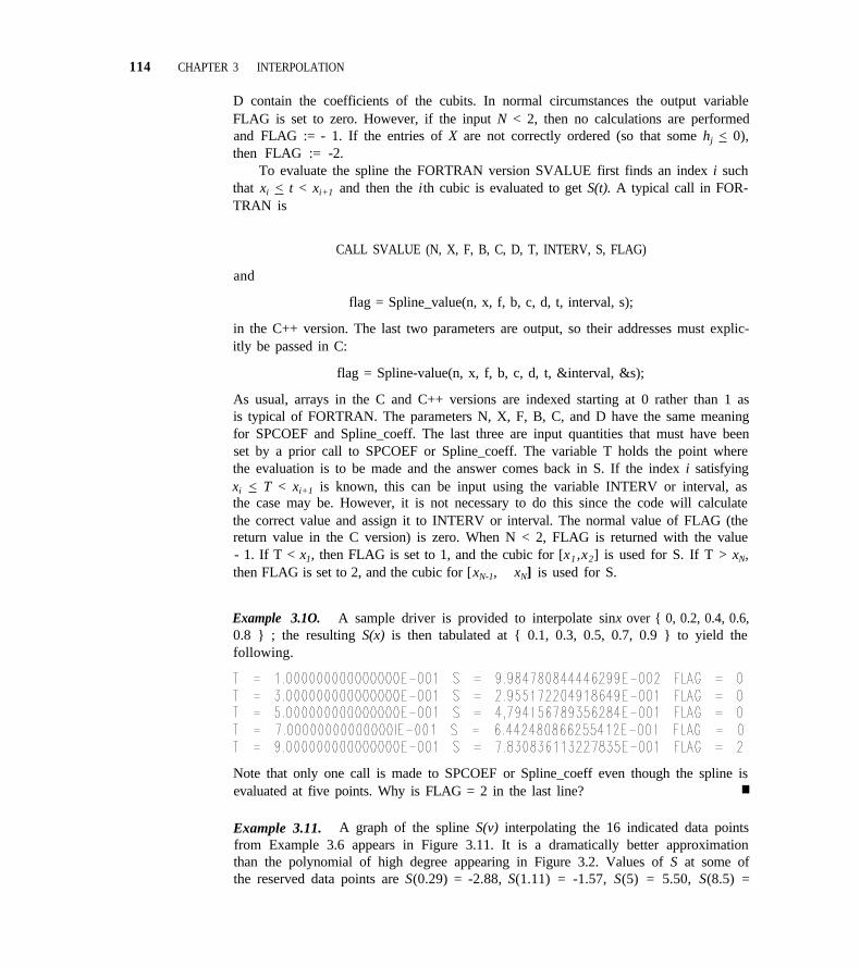
114 CHAPTER 3 INTERPOLATION
D contain the coefficients of the cubits. In normal circumstances the output variableFLAG is set to zero. However, if the input N < 2, then no calculations are performedand FLAG := - 1. If the entries of X are not correctly ordered (so that some hj < 0),then FLAG := -2.
To evaluate the spline the FORTRAN version SVALUE first finds an index i suchthat xi < t < xi+1 and then the ith cubic is evaluated to get S(t). A typical call in FOR-TRAN is
CALL SVALUE (N, X, F, B, C, D, T, INTERV, S, FLAG)
and
flag = Spline_value(n, x, f, b, c, d, t, interval, s);
in the C++ version. The last two parameters are output, so their addresses must explic-itly be passed in C:
flag = Spline-value(n, x, f, b, c, d, t, &interval, &s);
As usual, arrays in the C and C++ versions are indexed starting at 0 rather than 1 asis typical of FORTRAN. The parameters N, X, F, B, C, and D have the same meaningfor SPCOEF and Spline_coeff. The last three are input quantities that must have beenset by a prior call to SPCOEF or Spline_coeff. The variable T holds the point wherethe evaluation is to be made and the answer comes back in S. If the index i satisfyingxi < T < xi+1 is known, this can be input using the variable INTERV or interval, asthe case may be. However, it is not necessary to do this since the code will calculatethe correct value and assign it to INTERV or interval. The normal value of FLAG (thereturn value in the C version) is zero. When N < 2, FLAG is returned with the value- 1. If T < x1, then FLAG is set to 1, and the cubic for [x1 ,x2] is used for S. If T > xN,then FLAG is set to 2, and the cubic for [xN-1, xN] is used for S.
Example 3.1O. A sample driver is provided to interpolate sinx over { 0, 0.2, 0.4, 0.6,0.8 } ; the resulting S(x) is then tabulated at { 0.1, 0.3, 0.5, 0.7, 0.9 } to yield thefollowing.
Note that only one call is made to SPCOEF or Spline_coeff even though the spline isevaluated at five points. Why is FLAG = 2 in the last line? n
Example 3.11. A graph of the spline S(v) interpolating the 16 indicated data pointsfrom Example 3.6 appears in Figure 3.11. It is a dramatically better approximationthan the polynomial of high degree appearing in Figure 3.2. Values of S at some ofthe reserved data points are S(0.29) = -2.88, S(1.11) = -1.57, S(5) = 5.50, S(8.5) =
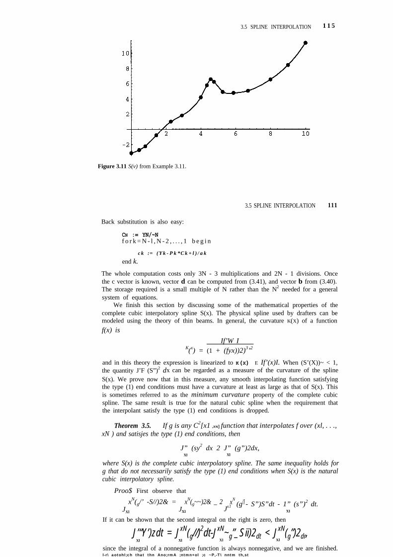
1 1 53.5 SPLINE INTERPOLATION
Figure 3.11 S(v) from Example 3.11.
3.5 SPLINE INTERPOLATION 111
Back substitution is also easy:
CN := YN/~Nf o r k = N - l , N - 2 , . . . , 1 b e g i n
c k : = ( Y k - P k * C k + l ) / a k
end k.
The whole computation costs only 3N - 3 multiplications and 2N - 1 divisions. Oncethe c vector is known, vector d can be computed from (3.41), and vector b from (3.40).The storage required is a small multiple of N rather than the N2 needed for a generalsystem of equations.
We finish this section by discussing some of the mathematical properties of thecomplete cubic interpolatory spline S(x). The physical spline used by drafters can bemodeled using the theory of thin beams. In general, the curvature K(X) of a function
f(x) is
If’W IK(x) = (1 + (fyx))2)3’2
and in this theory the expression is linearized to K(X) E If’(x)I. When (S’(X))~ < 1,the quantity J’F (S”)2 dx can be regarded as a measure of the curvature of the splineS(x). We prove now that in this measure, any smooth interpolating function satisfyingthe type (1) end conditions must have a curvature at least as large as that of S(x). Thisis sometimes referred to as the minimum curvature property of the complete cubicspline. The same result is true for the natural cubic spline when the requirement thatthe interpolant satisfy the type (1) end conditions is dropped.
Theorem 3.5. If g is any C2[x1 ,XN] function that interpolates f over (xl, . . .,xN ) and satisjes the type (1) end conditions, then
J” (sy2 dx 2 J” (g”)2dx,Xl Xl
where S(x) is the complete cubic interpolatory spline. The same inequality holds forg that do not necessarily satisfy the type (1) end conditions when S(x) is the naturalcubic interpolatory spline.
Proo$ First observe that
JxN(g/’ -S//)2& =
JxN(g~~)2& _ 2
Xl Xl JxN /I
x1 (g - S”)S”dt - 1” (s”)2 dt.Xl
If it can be shown that the second integral on the right is zero, then
J’“Y’)zdt = JxN(g//)2dt-JxN~g”_Sii)2dt < JxN(g”)2dr,
Xl Xl Xl Xl
since the integral of a nonnegative function is always nonnegative, and we are finished.l-r\ aotohl;ch that thn Ano;rmA ;ntmn+ol ;c ~P,-T\ nntm th,st
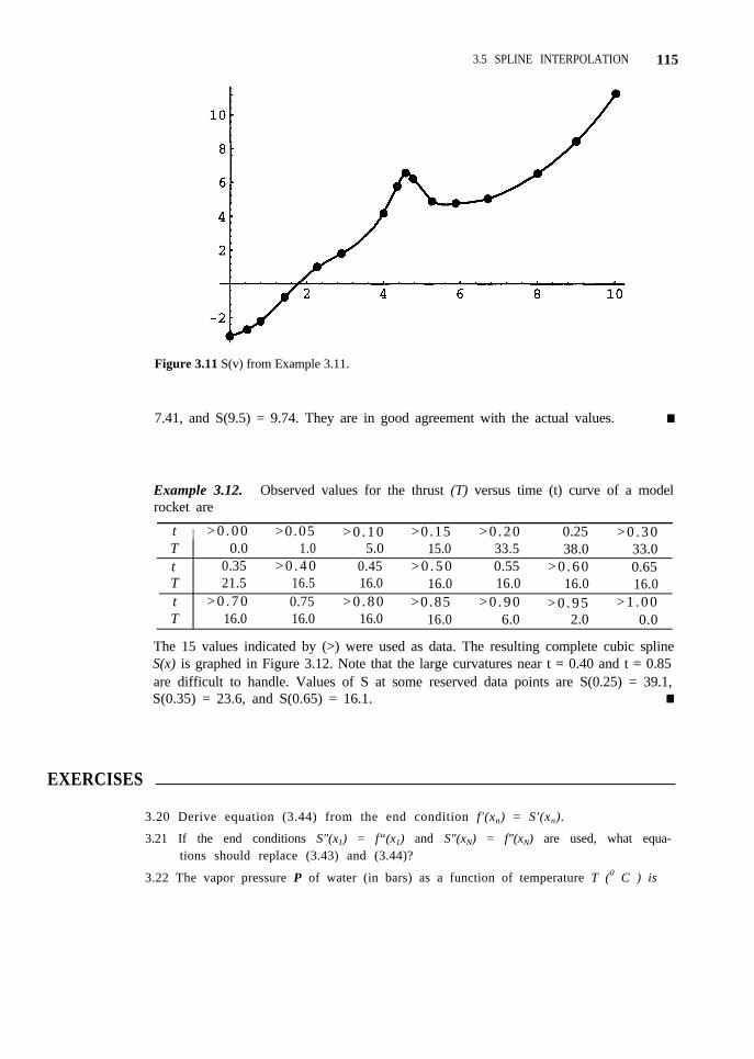
EXERCISES
3.5 SPLINE INTERPOLATION 115
Figure 3.11 S(v) from Example 3.11.
7.41, and S(9.5) = 9.74. They are in good agreement with the actual values. n
Example 3.12. Observed values for the thrust (T) versus time (t) curve of a modelrocket are
t I > 0 . 0 0 >0.05 > 0 . 1 0 >0.15 > 0 . 2 0 0.25 > 0 . 3 0T 0.0 1.0 5.0 15.0 33.5 38.0 33.0t 0.35 > 0 . 4 0 0.45 > 0 . 5 0 0.55 > 0 . 6 0 0.65T 21.5 16.5 16.0 16.0 16.0 16.0 16.0t > 0 . 7 0 0.75 > 0 . 8 0 >0.85 > 0 . 9 0 > 0 . 9 5 > 1 . 0 0T 16.0 16.0 16.0 16.0 6.0 2.0 0.0
The 15 values indicated by (>) were used as data. The resulting complete cubic splineS(x) is graphed in Figure 3.12. Note that the large curvatures near t = 0.40 and t = 0.85are difficult to handle. Values of S at some reserved data points are S(0.25) = 39.1,S(0.35) = 23.6, and S(0.65) = 16.1. n
3.20 Derive equation (3.44) from the end condition f'(xn) = S'(xn).
3.21 If the end conditions S"(x1) = f“(x1) and S"(xN) = f"(xN) are used, what equa-tions should replace (3.43) and (3.44)?
3.22 The vapor pressure P of water (in bars) as a function of temperature T (0 C ) is
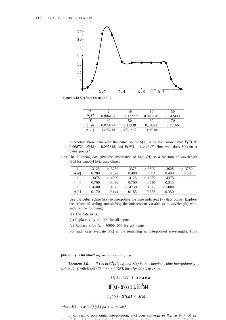
116 CHAPTER 3 INTERPOLATION
Figure 3.12 S(t) from Example 3.12.
0 10 20 300.006107 0.012277 0.023378 0.042433
T 40 50 60 70p m 0.073774 0.12338 0.19924 0.31166p k ) 0.47364 80 0.70112 90 1.01325 100
Interpolate these data with the cubic spline S(x). It is also known that P(5) =0.008721, P(45) = 0.095848, and P(95) = 0.84528. How well does S(x) do atthese points?
3.23 The following data give the absorbance of light (A) as a function of wavelength(3L) for vanadyl D-tartrate dimer.
h > 3125 > 3250 3375 > 3500 3625 > 3750A@) 0.700 0.572 0.400 0.382 0.449 0.560
h 3875 > 4000 4125 > 4250 43754 v 0.769 0.836 0.750 0.530 0.315
h > 4500 4625 > 4750 4875 > 5000A(U 0.170 0.144 0.183 0.252 0.350
Use the cubic spline S(x) to interpolate the nine indicated (>) data points. Explorethe effects of scaling and shifting the independent variable (x = wavelength) witheach of the following.
(a) The data as is.
(b) Replace x by x/ 1000 for all inputs.
(c) Replace x by (x - 4000)/1000 for all inputs.
For each case evaluate S(x) at the remaining noninterpolated wavelengths. How
Theorem 3.6. If f is in C4[x1, xN], and S(x) is the complete cubic interpolator-yspline for f with knots {XI < - - - < XN), then for any x in [xl ,XN]
I f ( $ - - W I I & h 4 M 4
If’(x) - S’(x) 1 L hh3M41 f”(x) - S”(x)1 < ;h2M4,
where M4 = max If t4) (x) I for x in [xl ,xN].
In contrast to polynomial interpolation, S(x) does converge to f(x) as N + 00 asI - - - _ ^ I - r \ q - t - I - 1 , , & , , , l _ ^ _ _ _ 1 I , , , . , & : , . , , , c C L , , , , I : - - , l , , - , . . - _ * - - _ ^ c - C L ,
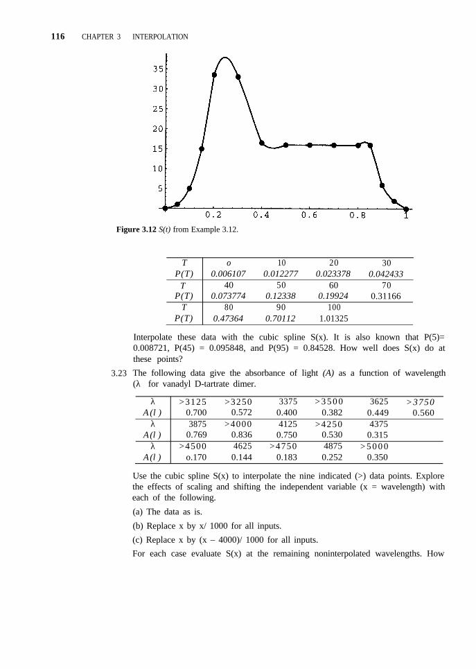
116 CHAPTER 3 INTERPOLATION
Figure 3.12 S(t) from Example 3.12.
T o 10 20 30P(T) 0.006107 0.012277 0.023378 0.042433
T 40 50 60 70P(T) 0.073774 0.12338 0.19924 0.31166
T 80 90 100P(T) 0.47364 0.70112 1.01325
3.23
Interpolate these data with the cubic spline S(x). It is also known that P(5)=0.008721, P(45) = 0.095848, and P(95) = 0.84528. How well does S(x) do atthese points?
The following data give the absorbance of light (A) as a function of wavelength(λ) for vanadyl D-tartrate dimer.
λ >3125 >3250 3375 > 3 5 0 0 3625Α(λ)
>37500.700 0.572 0.400 0.382 0.449 0.560
λ 3875 >4000 4125 >4250 4375Α(λ) 0.769 0.836 0.750 0.530 0.315
λ >4500 4625 >4750 4875 > 5 0 0 0Α(λ) o.170 0.144 0.183 0.252 0.350
Use the cubic spline S(x) to interpolate the nine indicated (>) data points. Explorethe effects of scaling and shifting the independent variable (x = wavelength) witheach of the following.
(a) The data as is.
(b) Replace x by x/ 1000 for all inputs.
(c) Replace x by (x – 4000)/ 1000 for all inputs.
For each case evaluate S(x) at the remaining noninterpolated wavelengths. How
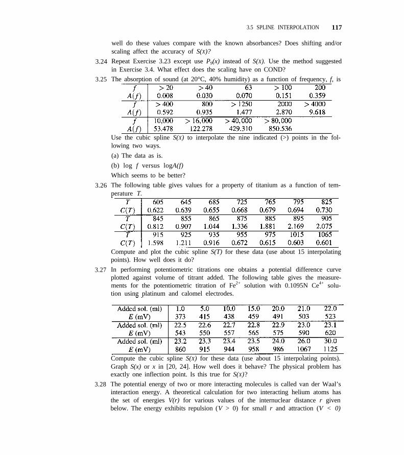
3.5 SPLINE INTERPOLATION 117
3.24
3.25
3.26
3.27
3.28
well do these values compare with the known absorbances? Does shifting and/orscaling affect the accuracy of S(X)?
Repeat Exercise 3.23 except use P9(x) instead of S(X). Use the method suggestedin Exercise 3.4. What effect does the scaling have on COND?
The absorption of sound (at 20°C, 40% humidity) as a function of frequency, f, is
Use the cubic spline S(X) to interpolate the nine indicated (>) points in the fol-lowing two ways.
(a) The data as is.
(b) log f versus logA(f)
Which seems to be better?
The following table gives values for a property of titanium as a function of tem-perature T.
Compute and plot the cubic spline S(T) for these data (use about 15 interpolatingpoints). How well does it do?
In performing potentiometric titrations one obtains a potential difference curveplotted against volume of titrant added. The following table gives the measure-ments for the potentiometric titration of Fe2+ solution with 0.1095N Ce4+ solu-tion using platinum and calomel electrodes.
Compute the cubic spline S(X) for these data (use about 15 interpolating points).Graph S(x) or x in [20, 24]. How well does it behave? The physical problem hasexactly one inflection point. Is this true for S(X)?
The potential energy of two or more interacting molecules is called van der Waal’sinteraction energy. A theoretical calculation for two interacting helium atoms hasthe set of energies V(r) for various values of the internuclear distance r givenbelow. The energy exhibits repulsion (V > 0) for small r and attraction (V < 0)
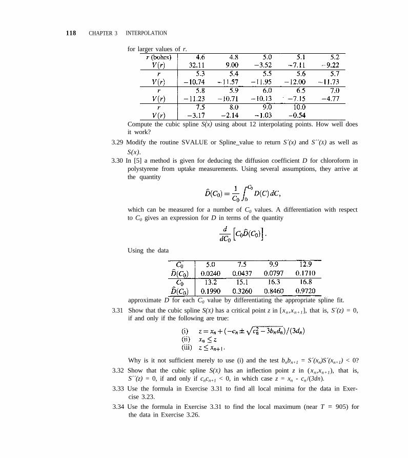
118 CHAPTER 3 INTERPOLATION
for larger values of r.
Compute the cubic spline S(x) using about 12 interpolating points. How well doesit work?
3.29 Modify the routine SVALUE or Spline_value to return S´(x) and S´´(X) as well as
S(x).3.30 In [5] a method is given for deducing the diffusion coefficient D for chloroform in
polystyrene from uptake measurements. Using several assumptions, they arrive atthe quantity
which can be measured for a number of C0 values. A differentiation with respectto C0 gives an expression for D in terms of the quantity
Using the data
approximate D for each C0 value by differentiating the appropriate spline fit.
3.31 Show that the cubic spline S(X) has a critical point z in [xn ,xn+1], that is, S´(z) = 0,if and only if the following are true:
Why is it not sufficient merely to use (i) and the test bnbn+1 = S´(xn)S´(xn+1) < 0?
3.32 Show that the cubic spline S(X) has an inflection point z in (xn,xn+1), that is,S´´(z) = 0, if and only if cncn+1 < 0, in which case z = xn - cn /(3dn).
3.33 Use the formula in Exercise 3.31 to find all local minima for the data in Exer-cise 3.23.
3.34 Use the formula in Exercise 3.31 to find the local maximum (near T = 905) forthe data in Exercise 3.26.
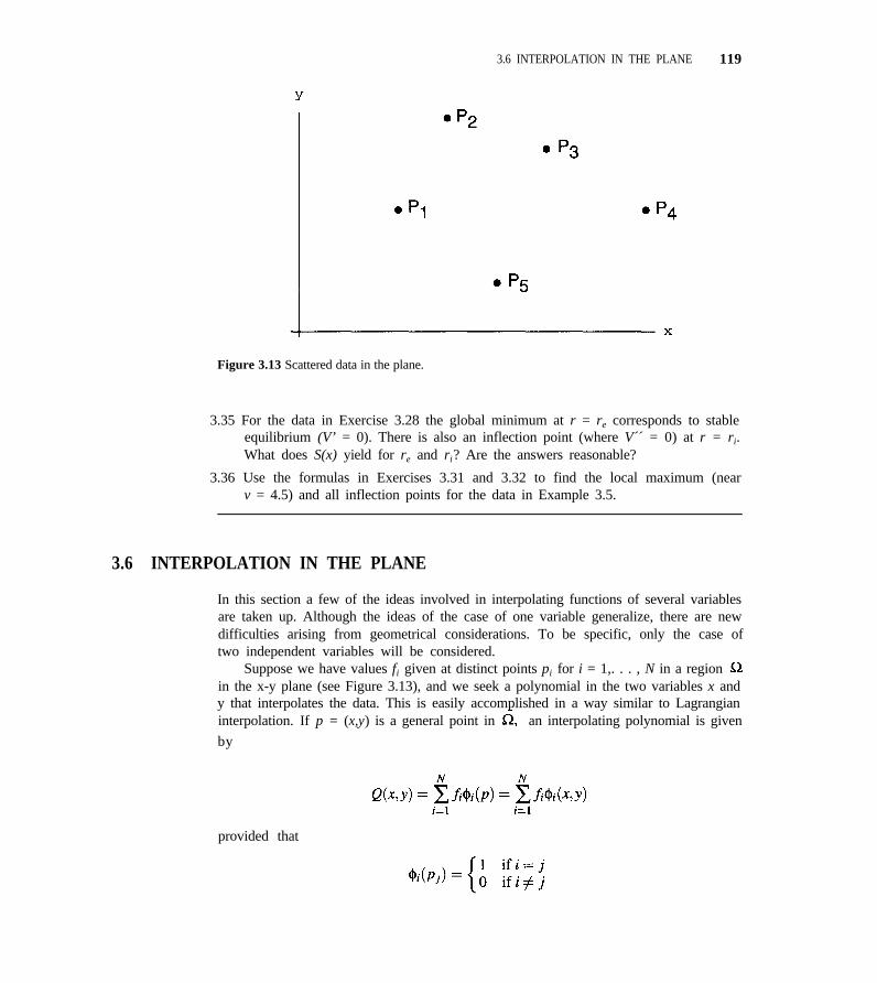
3.6 INTERPOLATION IN THE PLANE 119
Figure 3.13 Scattered data in the plane.
3.35 For the data in Exercise 3.28 the global minimum at r = re corresponds to stableequilibrium (V’ = 0). There is also an inflection point (where V´´ = 0) at r = ri.What does S(x) yield for re and ri? Are the answers reasonable?
3.36 Use the formulas in Exercises 3.31 and 3.32 to find the local maximum (nearv = 4.5) and all inflection points for the data in Example 3.5.
3.6 INTERPOLATION IN THE PLANE
In this section a few of the ideas involved in interpolating functions of several variablesare taken up. Although the ideas of the case of one variable generalize, there are newdifficulties arising from geometrical considerations. To be specific, only the case oftwo independent variables will be considered.
Suppose we have values fi given at distinct points pi for i = 1,. . . , N in a region in the x-y plane (see Figure 3.13), and we seek a polynomial in the two variables x andy that interpolates the data. This is easily accomplished in a way similar to Lagrangianinterpolation. If p = (x,y) is a general point in an interpolating polynomial is given
by
provided that
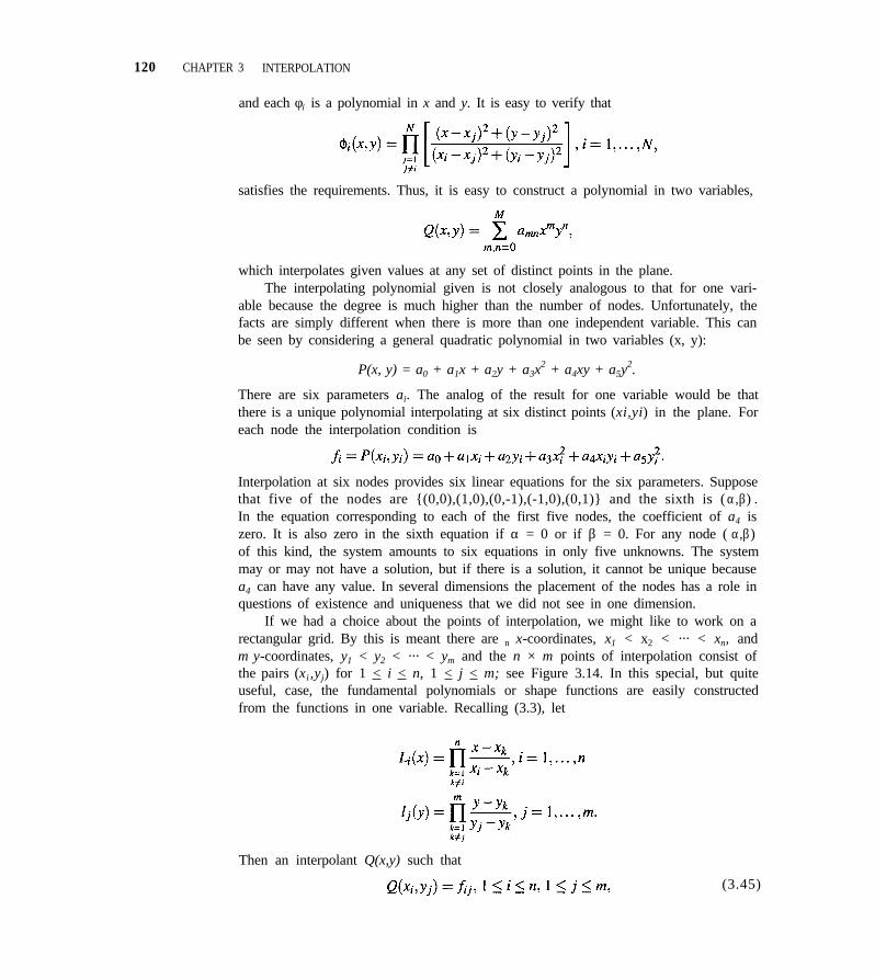
120 CHAPTER 3 INTERPOLATION
and each φi is a polynomial in x and y. It is easy to verify that
satisfies the requirements. Thus, it is easy to construct a polynomial in two variables,
which interpolates given values at any set of distinct points in the plane.The interpolating polynomial given is not closely analogous to that for one vari-
able because the degree is much higher than the number of nodes. Unfortunately, thefacts are simply different when there is more than one independent variable. This canbe seen by considering a general quadratic polynomial in two variables (x, y):
P(x, y) = a0 + a1x + a2y + a3x2 + a4xy + a5y
2.
There are six parameters ai. The analog of the result for one variable would be thatthere is a unique polynomial interpolating at six distinct points (xi,yi) in the plane. Foreach node the interpolation condition is
Interpolation at six nodes provides six linear equations for the six parameters. Supposethat five of the nodes are {(0,0),(1,0),(0,-1),(-1,0),(0,1)} and the sixth is ( α,β) .In the equation corresponding to each of the first five nodes, the coefficient of a4 iszero. It is also zero in the sixth equation if α = 0 or if β = 0. For any node ( α,β)of this kind, the system amounts to six equations in only five unknowns. The systemmay or may not have a solution, but if there is a solution, it cannot be unique becausea4 can have any value. In several dimensions the placement of the nodes has a role inquestions of existence and uniqueness that we did not see in one dimension.
If we had a choice about the points of interpolation, we might like to work on arectangular grid. By this is meant there are n x-coordinates, x1 < x2 < ··· < xn, andm y-coordinates, y1 < y2 < ··· < ym and the n × m points of interpolation consist ofthe pairs (xi ,yj) for 1 < i < n, 1 < j < m; see Figure 3.14. In this special, but quiteuseful, case, the fundamental polynomials or shape functions are easily constructedfrom the functions in one variable. Recalling (3.3), let
Then an interpolant Q(x,y) such that
(3.45)
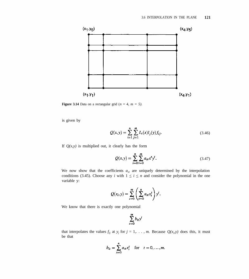
3.6 INTERPOLATION IN THE PLANE 121
Figure 3.14 Data on a rectangular grid (n = 4, m = 5).
is given by
(3.46)
If Q(x,y) is multiplied out, it clearly has the form
(3.47)
We now show that the coefficients ast are uniquely determined by the interpolationconditions (3.45). Choose any i with 1 < i < n and consider the polynomial in the onevariable y:
We know that there is exactly one polynomial
that interpolates the values fij at yj for j = 1,. . . , m. Because Q(xi,y) does this, it mustbe that

122 CHAPTER 3 INTERPOLATION
This equation holds for each i. Now choose a t with 0 < t < m. There is exactly onepolynomial
such that
R(xi) = bit for i = l, . . . ,n.
Because the polynomial
does this, it must be the case that cst = ast for 0 < s < n and for any 0 < t < m. Thus thecoefficients ast are uniquely determined by the interpolation coefficients as we wantedto show.
As a simple example, let us consider interpolation at the four comers of a rectan-gle: (x1,yl) (xl,y2), (x2 ,y1) (x2 ,y2).
(3.48)
Figure 3.15 displays a typical interpolant for n = 4 and m = 3.Interpolants constructed in this way are called tensor product interpolants. The
example (3.48) is said to be a bilinear interpolant over a rectangle because it has theform
a00 + a10x + a01y + a11xy, (3.49)
that is, it is linear in each variable when the other is held fixed. The general first degreepolynomial has the form (3.49) with a11 = 0. A biquadratic has the form
while the general second degree polynomial has here a21 = a22 = a12 = 0. General-izations to bicubic versus cubic and higher degrees should be clear.
In studying how well a function of two variables is approximated by a particularkind of interpolating polynomial, a critical matter is the highest degree for which theapproximation is exact. For example, in the rectangle of Figure 3.16, we can inter-polate at the nine indicated points using a biquadratic. However, it is exact only forsecond degree polynomials in spite of the presence of the higher degree terms x2y, yx2,and x2y2. In fact only six interpolating points are needed to construct a quadratic inter-polating polynomial that is exact to second degree. It is not at all clear how to choose
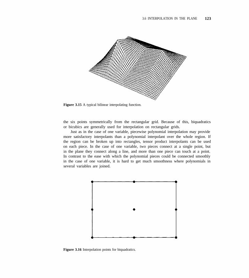
3.6 INTERPOLATION IN THE PLANE 123
Figure 3.15 A typical bilinear interpolating function.
the six points symmetrically from the rectangular grid. Because of this, biquadraticsor bicubics are generally used for interpolation on rectangular grids.
Just as in the case of one variable, piecewise polynomial interpolation may providemore satisfactory interpolants than a polynomial interpolant over the whole region. Ifthe region can be broken up into rectangles, tensor product interpolants can be usedon each piece. In the case of one variable, two pieces connect at a single point, butin the plane they connect along a line, and more than one piece can touch at a point.In contrast to the ease with which the polynomial pieces could be connected smoothlyin the case of one variable, it is hard to get much smoothness where polynomials inseveral variables are joined.
Figure 3.16 Interpolation points for biquadratics.
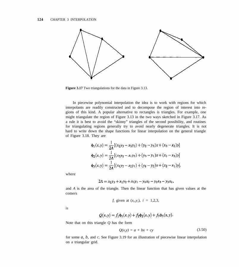
124 CHAPTER 3 INTERPOLATION
Figure 3.17 Two triangulations for the data in Figure 3.13.
In piecewise polynomial interpolation the idea is to work with regions for whichinterpolants are readily constructed and to decompose the region of interest into re-gions of this kind. A popular alternative to rectangles is triangles. For example, onemight triangulate the region of Figure 3.13 in the two ways sketched in Figure 3.17. Asa rule it is best to avoid the “skinny” triangles of the second possibility, and routinesfor triangulating regions generally try to avoid nearly degenerate triangles. It is nothard to write down the shape functions for linear interpolation on the general triangleof Figure 3.18. They are
where
and A is the area of the triangle. Then the linear function that has given values at thecomers
is
fi given at (xi,yi), i = 1,2,3,
Note that on this triangle Q has the form
Q(x,y) = a + bx + cy (3.50)
for some a, b, and C. See Figure 3.19 for an illustration of piecewise linear interpolationon a triangular grid.
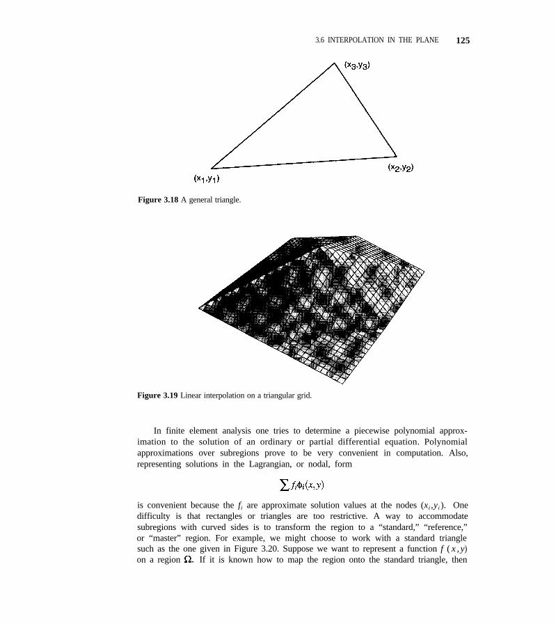
3.6 INTERPOLATION IN THE PLANE 125
Figure 3.18 A general triangle.
Figure 3.19 Linear interpolation on a triangular grid.
In finite element analysis one tries to determine a piecewise polynomial approx-imation to the solution of an ordinary or partial differential equation. Polynomialapproximations over subregions prove to be very convenient in computation. Also,representing solutions in the Lagrangian, or nodal, form
is convenient because the fi are approximate solution values at the nodes (xi ,yi ). Onedifficulty is that rectangles or triangles are too restrictive. A way to accommodatesubregions with curved sides is to transform the region to a “standard,” “reference,”or “master” region. For example, we might choose to work with a standard trianglesuch as the one given in Figure 3.20. Suppose we want to represent a function f ( x , y)on a region If it is known how to map the region onto the standard triangle, then
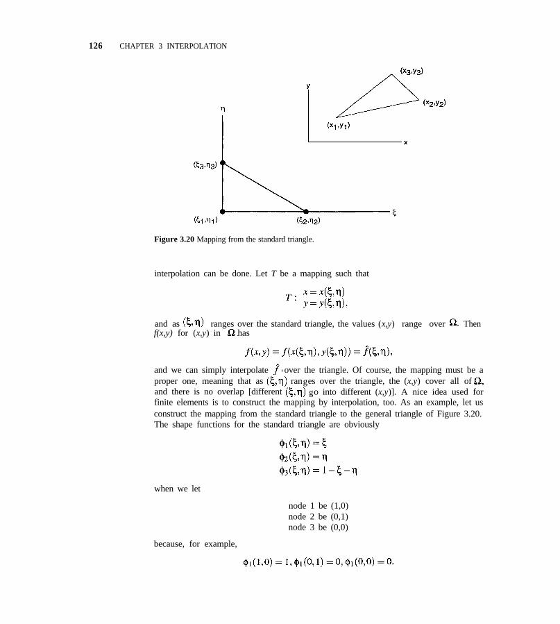
126 CHAPTER 3 INTERPOLATION
Figure 3.20 Mapping from the standard triangle.
interpolation can be done. Let T be a mapping such that
and as ranges over the standard triangle, the values (x,y) range over Thenf(x,y) for (x,y) in has
and we can simply interpolate over the triangle. Of course, the mapping must be aproper one, meaning that as ranges over the triangle, the (x,y) cover all ofand there is no overlap [different go into different (x,y)]. A nice idea used forfinite elements is to construct the mapping by interpolation, too. As an example, let usconstruct the mapping from the standard triangle to the general triangle of Figure 3.20.The shape functions for the standard triangle are obviously
when we let
node 1 be (1,0)node 2 be (0,1)node 3 be (0,0)
because, for example,
3.6 INTERPOLATION IN THE PLANE 127
Interpolating x we have
and, similarly,
In this particular case the mapping carries straight lines into straight lines and thereis no difficulty about a proper mapping. If higher degree interpolation were used, thetriangle would be mapped into a region with curved sides. Roughly speaking, if theregion is not too different from a triangle, the mapping will be proper. Continuingwith the example, suppose we interpolate the fi by the same basis functions used toconstruct the mapping. The interpolant Q(x,y) is
If we were to solve the relation to get the inverse mapping
and eliminate and η in this interpolant, we would get the expression earlier for thebilinear interpolant. This seems a complicated way to get a simple result. The virtue ofthe procedure is that interpolation is done on regions with curved boundaries by trans-forming them to a simple, standard region for which interpolation is comparativelyeasy. In finite element computations it is found that the process is easily programmedand very powerful. All we aim to do here is sketch the process. For details the readermay consult one of the great many books devoted to finite elements. The books span agreat range of mathematical sophistication; a good introduction is [1].
EXERCISES
3.37 The formula (3.48) could be called a Lagrange form 3.38 Show that Q(x,y), which is a quadratic polynomial inof the bilinear interpolating polynomial; consider the x and y [generalizing (3.50)], has six coefficients. On a“Newton form” triangle, its interpolating points are usually chosen to
be the three triangle vertices and the three edge mid-points. For the triangle with vertices (0,0), (1,0), and
Solve for a, b, c, and d so that Q interpolates a (0,l) compute the shape function that is one at (0,0)function f(x,y) at the four corners. As in (3.48) let and zero at the remaining five interpolating points.
128 CHAPTER 3 INTERPOLATION
3.7 CASE STUDY 3
This case study has two parts, one applying continuous splines and the other, smoothsplines. Integrals of the form
with finite a and b are called finite Fourier integrals. For large ω such integrals presentspecial difficulties for numerical methods because of the rapid oscillation of the inte-grand. Filon’s method [8] for approximating finite Fourier integrals will be developedhere by means of a continuous spline. Accurate evaluation of the coefficients of themethod was discussed in Chapter 1. Other aspects of the task will be discussed inChapter 5. The second part of the case study takes up the use of smooth splines forfitting data with curves instead of functions.
Broadly speaking, Filon approximates finite Fourier integrals in a manner like thatused in Chapter 5 for integrals of the form
when w(x) presents some difficulty. Namely, first approximate f(x) with a convenientfunction S(x) and then compute analytically
as an approximation to the desired integral. In detail there are important differencesbecause here the weight function w(x) does not have one sign and oscillates rapidlyfor large frequencies ω. Also, the approach of Chapter 5 would apply to particularω, and we would like a method that can be applied conveniently for any ω. Insightis provided by a classic technique of applied mathematics for approximating Fourierintegrals when w is “large.” If derivatives of f(x) are available, asymptotic approxi-mations can be obtained by means of integration by parts. For example, integrating byparts twice gives
where
If M1 is a bound on the magnitude of f´(x), then
that is, R(ω) is 0(ω−2) as Accordingly, the asymptotic approximation
3.7 CASE STUDY 3 129
is accurate to 0(ω-2). However, the integral itself ordinarily goes to zero like ω - 1 ,so the relative error is ordinarily only 0( ω-1). The situation is typical of classicalasymptotic approximation of integrals. The bigger w is, the better the asymptotic ap-proximation and the more difficult the integral is for conventional numerical methods.On the other hand, for a given w, the asymptotic approximation may not be sufficientlyaccurate and there is no easy way to improve it. When w is “small,” finite Fourier inte-grals are easy for conventional numerical methods, and when w is “large,” asymptoticapproximations are satisfactory. Filon’s method provides a way to compute accurateintegrals when w is of moderate size.
Filon divides the interval [a,b] into 2N subintervals of equal length h. Let us definexj = a + jh for j = 0, . . . ,2N. The function f(x) is approximated by a continuous splineS(x) that is a quadratic polynomial on each [x 2 m , x m + 2 ] defined there by interpolationto f(xj) for j = 2m, 2m + 1,2m + 2. Each of the integrals in the approximation
can be evaluated analytically by integration by parts. A lengthy calculation results inFilon’s method:
Here θ = ωh and
Also,
There is a similar approximation when cosine is replaced by sine. The formula is
The coefficients α, β, γ are the same, and Se and So are like Ce and Co with the cosinesreplaced by sines.
Using the results developed in this chapter for the error of interpolation, it is easyto bound the error of Filon’s method. On each subinterval [x 2 m , x 2 m + 2 ], S(x) is aquadratic interpolant to f(x). If M3 is a bound on the third derivative of f(x) onall of [a,b], we found that
130 CHAPTER 3 INTERPOLATION
uniformly for a < x < b. Then
This is a bound on the absolute error that depends on f(x) and the sampling intervalh, but not on ω. If we want a meaningful result for “large” ω, we have to take intoaccount that the integral is 0(ω-l). This leads to a bound on the relative error that is0 ( θ- 1 h 4 ) .
In a subsection of Chapter 5 about applying a general-purpose code to problemswith oscillatory integrands, the example
is discussed. The function f(x) = l/(1 + x2) ought to be approximated well by aquadratic interpolatory spline with a relatively crude mesh, so Filon’s method oughtto be quite effective. A matter not usually discussed with Filon’s method is how toestimate the accuracy of the result. One way to proceed is to compute a result that webelieve to be more accurate and estimate the error of the less accurate result by com-parison. If the accuracy is acceptable, often the more accurate result is the one taken asthe answer. Inspection of the formulas shows that if h, or equivalently θ, is halved, wecan reuse all the evaluations of f, sin(x), and cos(x) made in the first approximationto keep down the cost. According to the bounds, the error should be reduced enoughby halving h to get a good estimate of the error by comparison. Using Filon’s methodwith θ = 0.4, we obtained an approximate integral of 0.04566373122996. Halving θresulted in the approximation 0.04566373690838. Estimating the accuracy by com-parison suggests that we have an answer with an error smaller than 6 × 10⁻⁹. Reuseof the function evaluations by virtue of halving θ holds the cost to 315 evaluationsof the integrand. The quadrature code Adapt developed in Chapter 5 asks the userto specify the accuracy desired. Using the code in the manner outlined in that chap-ter and experimenting some with the error tolerances, we obtained an approximation0.04566373866324 with an estimated error of about -1.6 × 10⁻⁹. This cost 1022evaluations of the integrand.
Let us now change the subject from applying a continuous spline to applying asmooth spline. In this chapter we have been looking at the approximation of functionsy = f(x), but sometimes we want to approximate curves. This will be discussed inthe plane for it will then be clear how to deal with a curve in three dimensions. Thebasic idea is to use a parametric representation (x(s),y(s)) for the curve and approx-imate independently the coordinate functions x(s) and y(s). The parameter s can beanything, but often in the theory it is taken to be arc length. Having chosen somehownodes si, i = l, . . . , N, we can interpolate the data xi = x(si) by a spline Sx(s) and like-wise the data yi = y(si) by a spline Sy(s). The curve (x(s),y(s)) is then approximatedby (Sx(s),Sy(s)). This yields a curve in the plane that passes through all the points(x(si),y(si)) in order. It is natural to use the smooth cubic spline of SPCOEF becauseit leads to a curve with continuous curvature, but if the data are sparse, we might haveto resort to the shape-preserving spline to get a curve of the expected shape. All thesecomputations are familiar except for the selection of the nodes si. One way to proceed
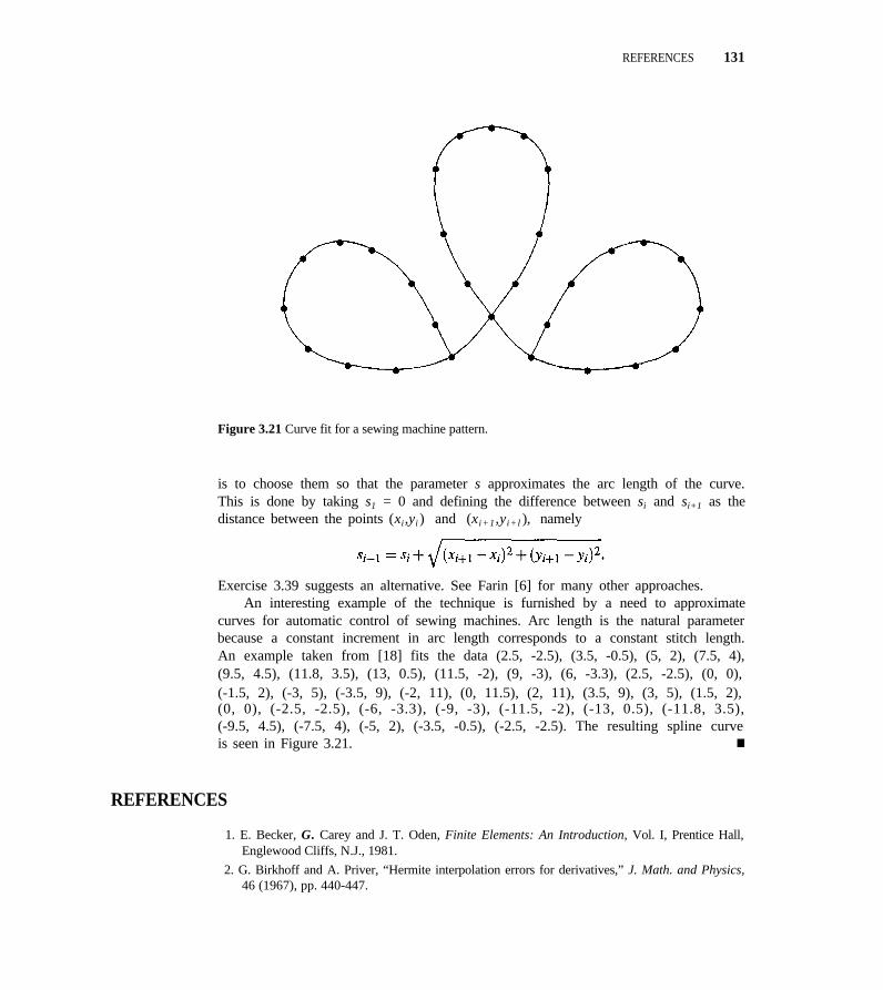
REFERENCES 131
Figure 3.21 Curve fit for a sewing machine pattern.
is to choose them so that the parameter s approximates the arc length of the curve.This is done by taking s1 = 0 and defining the difference between si and si+1 as thedistance between the points (xi,yi ) and (xi+1,yi+l ), namely
Exercise 3.39 suggests an alternative. See Farin [6] for many other approaches.An interesting example of the technique is furnished by a need to approximate
curves for automatic control of sewing machines. Arc length is the natural parameterbecause a constant increment in arc length corresponds to a constant stitch length.An example taken from [18] fits the data (2.5, -2.5), (3.5, -0.5), (5, 2), (7.5, 4),(9.5, 4.5), (11.8, 3.5), (13, 0.5), (11.5, -2), (9, -3), (6, -3.3), (2.5, -2.5), (0, 0),(-1.5, 2), (-3, 5), (-3.5, 9), (-2, 11), (0, 11.5), (2, 11), (3.5, 9), (3, 5), (1.5, 2),(0, 0), (-2.5, -2.5), (-6, -3.3), (-9, -3), (-11.5, -2), (-13, 0.5), (-11.8, 3.5),(-9.5, 4.5), (-7.5, 4), (-5, 2), (-3.5, -0.5), (-2.5, -2.5). The resulting spline curveis seen in Figure 3.21. n
REFERENCES
1. E. Becker, G. Carey and J. T. Oden, Finite Elements: An Introduction, Vol. I, Prentice Hall,Englewood Cliffs, N.J., 1981.
2. G. Birkhoff and A. Priver, “Hermite interpolation errors for derivatives,” J. Math. and Physics,46 (1967), pp. 440-447.
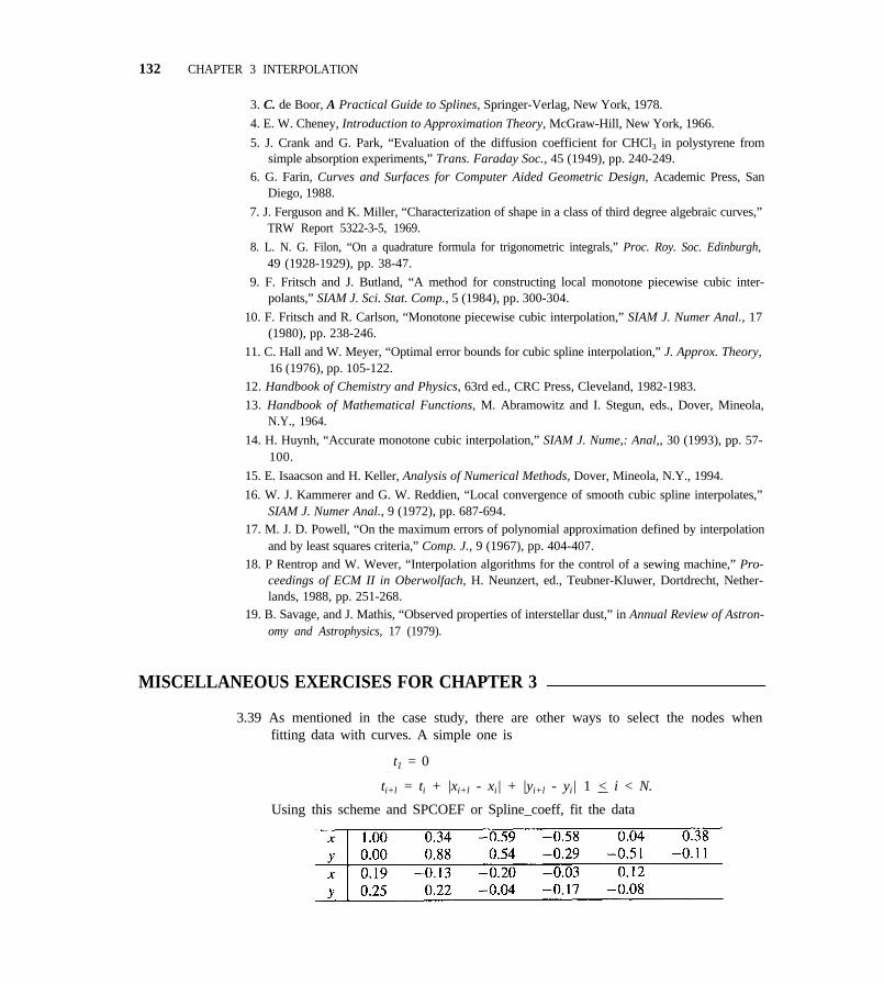
132 CHAPTER 3 INTERPOLATION
3. C. de Boor, A Practical Guide to Splines, Springer-Verlag, New York, 1978.
4. E. W. Cheney, Introduction to Approximation Theory, McGraw-Hill, New York, 1966.
5. J. Crank and G. Park, “Evaluation of the diffusion coefficient for CHCl3 in polystyrene fromsimple absorption experiments,” Trans. Faraday Soc., 45 (1949), pp. 240-249.
6. G. Farin, Curves and Surfaces for Computer Aided Geometric Design, Academic Press, SanDiego, 1988.
7. J. Ferguson and K. Miller, “Characterization of shape in a class of third degree algebraic curves,”TRW Report 5322-3-5, 1969.
8. L. N. G. Filon, “On a quadrature formula for trigonometric integrals,” Proc. Roy. Soc. Edinburgh,49 (1928-1929), pp. 38-47.
9. F. Fritsch and J. Butland, “A method for constructing local monotone piecewise cubic inter-polants,” SIAM J. Sci. Stat. Comp., 5 (1984), pp. 300-304.
10. F. Fritsch and R. Carlson, “Monotone piecewise cubic interpolation,” SIAM J. Numer Anal., 17(1980), pp. 238-246.
11. C. Hall and W. Meyer, “Optimal error bounds for cubic spline interpolation,” J. Approx. Theory,16 (1976), pp. 105-122.
12. Handbook of Chemistry and Physics, 63rd ed., CRC Press, Cleveland, 1982-1983.
13. Handbook of Mathematical Functions, M. Abramowitz and I. Stegun, eds., Dover, Mineola,N.Y., 1964.
14. H. Huynh, “Accurate monotone cubic interpolation,” SIAM J. Nume,: Anal,, 30 (1993), pp. 57-100.
15. E. Isaacson and H. Keller, Analysis of Numerical Methods, Dover, Mineola, N.Y., 1994.
16. W. J. Kammerer and G. W. Reddien, “Local convergence of smooth cubic spline interpolates,”SIAM J. Numer Anal., 9 (1972), pp. 687-694.
17. M. J. D. Powell, “On the maximum errors of polynomial approximation defined by interpolationand by least squares criteria,” Comp. J., 9 (1967), pp. 404-407.
18. P Rentrop and W. Wever, “Interpolation algorithms for the control of a sewing machine,” Pro-ceedings of ECM II in Oberwolfach, H. Neunzert, ed., Teubner-Kluwer, Dortdrecht, Nether-lands, 1988, pp. 251-268.
19. B. Savage, and J. Mathis, “Observed properties of interstellar dust,” in Annual Review of Astron-omy and Astrophysics, 17 (1979).
MISCELLANEOUS EXERCISES FOR CHAPTER 3
3.39 As mentioned in the case study, there are other ways to select the nodes whenfitting data with curves. A simple one is
t1 = 0
ti+l = ti + |xi+l - xi| + |yi+l - yi| 1 < i < N.
Using this scheme and SPCOEF or Spline_coeff, fit the data
133
Using SVALUE or Spline_value, evaluate at sufficiently many points to sketch asmooth curve in the xy plane.
3.40 Find a technique that gives a good fit to the model rocket data from Example 3.11.Interpolate the indicated (>) data and avoid undesirable oscillations.
3.41 Implement the shape-preserving cubic spline described in Section 3.5. Test it outon some of the data sets from this chapter, for example, Exercises 3.22, 3.25,and 3.27. Sketch the graph of H(x). Also try it on the nonmonotone data inExample 3.11, Exercise 3.26, and Exercise 3.28. How well does it do?
3.42 Implement the bilinear interpolating function Q(x,y) given in (3.48). Test it onseveral different functions and several different grids.
3.43 Implement the linear interpolating function Q(n,y) given in (3.50). Test it onseveral different functions and several different triangulations.
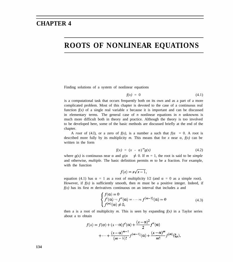
CHAPTER 4
ROOTS OF NONLINEAR EQUATIONS
Finding solutions of a system of nonlinear equations
f(x) = 0 (4.1)
is a computational task that occurs frequently both on its own and as a part of a morecomplicated problem. Most of this chapter is devoted to the case of a continuous realfunction f(x) of a single real variable x because it is important and can be discussedin elementary terms. The general case of n nonlinear equations in n unknowns ismuch more difficult both in theory and practice. Although the theory is too involvedto be developed here, some of the basic methods are discussed briefly at the end of thechapter.
A root of (4.l), or a zero of f(x), is a number a such that f(α) = 0. A root isdescribed more fully by its multiplicity m. This means that for x near α, f(x) can bewritten in the form
f(x) = (x - α) mg(x) (4.2)
where g(x) is continuous near α and g(α) 0. If m = 1, the root is said to be simpleand otherwise, multiple. The basic definition permits m to be a fraction. For example,with the function
equation (4.1) has α = 1 as a root of multiplicity l/2 (and α = 0 as a simple root).However, if f(x) is sufficiently smooth, then m must be a positive integer. Indeed, iff(x) has its first m derivatives continuous on an interval that includes a and
(4.3)
then a is a root of multiplicity m. This is seen by expanding f(x) in a Taylor seriesabout a to obtain
134
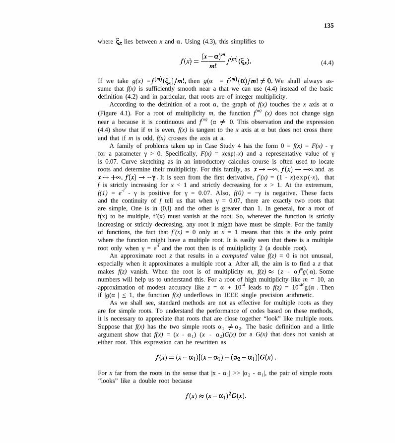
135
where lies between x and α. Using (4.3), this simplifies to
(4.4)
If we take g(x) = then g(α) = We shall always as-sume that f(x) is sufficiently smooth near a that we can use (4.4) instead of the basicdefinition (4.2) and in particular, that roots are of integer multiplicity.
According to the definition of a root α, the graph of f(x) touches the x axis at α(Figure 4.1). For a root of multiplicity m, the function f(m) (x) does not change signnear a because it is continuous and f(m) (α) 0. This observation and the expression(4.4) show that if m is even, f(x) is tangent to the x axis at α but does not cross thereand that if m is odd, f(x) crosses the axis at a.
A family of problems taken up in Case Study 4 has the form 0 = f(x) = F(x) - γfor a parameter γ > 0. Specifically, F(x) = xexp(-x) and a representative value of γis 0.07. Curve sketching as in an introductory calculus course is often used to locateroots and determine their multiplicity. For this family, as and as
It is seen from the first derivative, f´(x) = (1 - x) exp (-x), thatf is strictly increasing for x < 1 and strictly decreasing for x > 1. At the extremum,f(1) = e-l - γ is positive for γ = 0.07. Also, f(0) = −γ is negative. These factsand the continuity of f tell us that when γ = 0.07, there are exactly two roots thatare simple, One is in (0,l) and the other is greater than 1. In general, for a root off(x) to be multiple, f’(x) must vanish at the root. So, wherever the function is strictlyincreasing or strictly decreasing, any root it might have must be simple. For the familyof functions, the fact that f´(x) = 0 only at x = 1 means that this is the only pointwhere the function might have a multiple root. It is easily seen that there is a multipleroot only when γ = e-l and the root then is of multiplicity 2 (a double root).
An approximate root z that results in a computed value f(z) = 0 is not unusual,especially when it approximates a multiple root a. After all, the aim is to find a z thatmakes f(z) vanish. When the root is of multiplicity m, f(z) ( z - α)mg( α). Somenumbers will help us to understand this. For a root of high multiplicity like m = 10, anapproximation of modest accuracy like z = α + 10-4 leads to f(z) = 10-40g (α). Thenif |g(α)| < 1, the function f(z) underflows in IEEE single precision arithmetic.
As we shall see, standard methods are not as effective for multiple roots as theyare for simple roots. To understand the performance of codes based on these methods,it is necessary to appreciate that roots that are close together “look” like multiple roots.Suppose that f(x) has the two simple roots α1 α2. The basic definition and a littleargument show that f(x) = (x - α1) (x - α2)G(x) for a G(x) that does not vanish ateither root. This expression can be rewritten as
For x far from the roots in the sense that |x - α1| >> |α2 - α1|, the pair of simple roots“looks” like a double root because
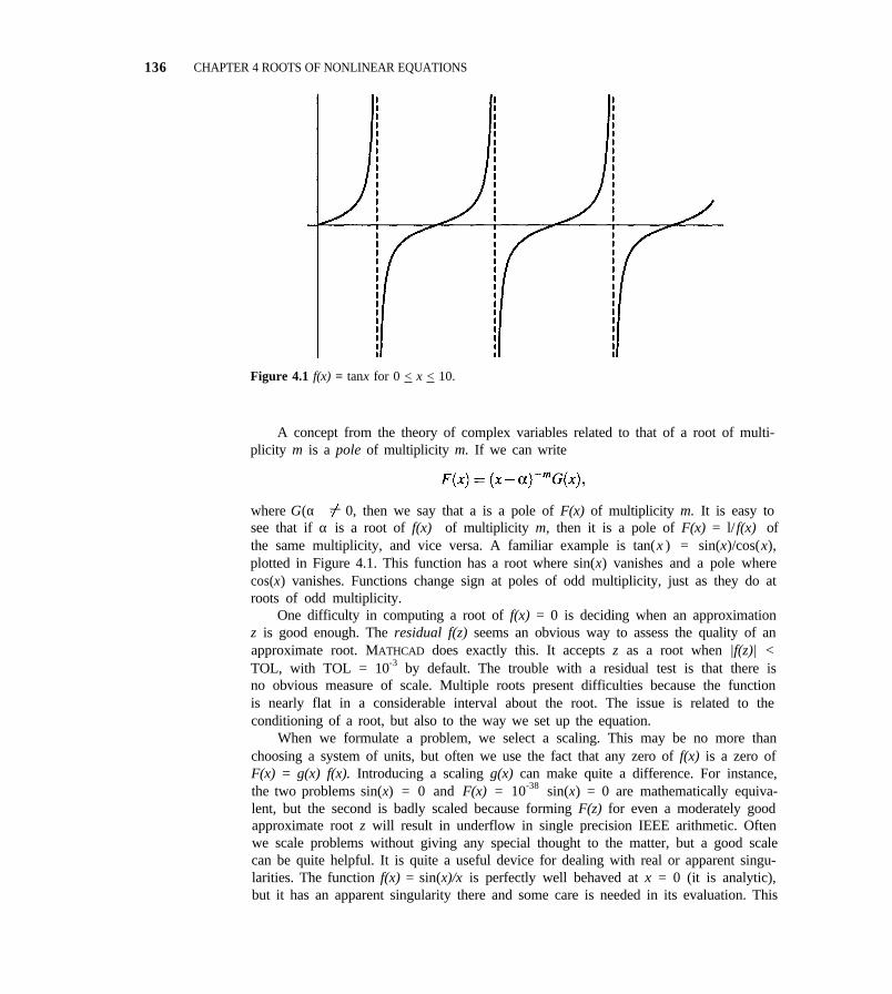
136 CHAPTER 4 ROOTS OF NONLINEAR EQUATIONS
Figure 4.1 f(x) = tanx for 0 < x < 10.
A concept from the theory of complex variables related to that of a root of multi-plicity m is a pole of multiplicity m. If we can write
where G(α) 0, then we say that a is a pole of F(x) of multiplicity m. It is easy tosee that if α is a root of f(x) of multiplicity m, then it is a pole of F(x) = l/ f(x) ofthe same multiplicity, and vice versa. A familiar example is tan(x ) = sin(x)/cos(x),plotted in Figure 4.1. This function has a root where sin(x) vanishes and a pole wherecos(x) vanishes. Functions change sign at poles of odd multiplicity, just as they do atroots of odd multiplicity.
One difficulty in computing a root of f(x) = 0 is deciding when an approximationz is good enough. The residual f(z) seems an obvious way to assess the quality of anapproximate root. MATHCAD does exactly this. It accepts z as a root when |f(z)| <TOL, with TOL = 10-3 by default. The trouble with a residual test is that there isno obvious measure of scale. Multiple roots present difficulties because the functionis nearly flat in a considerable interval about the root. The issue is related to theconditioning of a root, but also to the way we set up the equation.
When we formulate a problem, we select a scaling. This may be no more thanchoosing a system of units, but often we use the fact that any zero of f(x) is a zero ofF(x) = g(x) f(x). Introducing a scaling g(x) can make quite a difference. For instance,the two problems sin(x) = 0 and F(x) = 10-38 sin(x) = 0 are mathematically equiva-lent, but the second is badly scaled because forming F(z) for even a moderately goodapproximate root z will result in underflow in single precision IEEE arithmetic. Oftenwe scale problems without giving any special thought to the matter, but a good scalecan be quite helpful. It is quite a useful device for dealing with real or apparent singu-larities. The function f(x) = sin(x)/x is perfectly well behaved at x = 0 (it is analytic),but it has an apparent singularity there and some care is needed in its evaluation. This
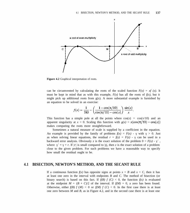
4.1 BISECTION, NEWTON’S METHOD, AND THE SECANT RULE 137
Figure 4.2 Graphical interpretation of roots.
can be circumvented by calculating the roots of the scaled function F(x) = xf (x). Itmust be kept in mind that as with this example, F(x) has all the roots of f(x), but itmight pick up additional roots from g(x). A more substantial example is furnished byan equation to be solved in an exercise:
This function has a simple pole at all the points where cos(x) = cos(π/10) and anapparent singularity at x = 0. Scaling this function with g(x) =makes computing the roots more straightforward.
Sometimes a natural measure of scale is supplied by a coefficient in the equation.An example is provided by the family of problems f(x) = F(x) - γ with γ > 0. Justas when solving linear equations, the residual r = f(z) = F(z) - γ can be used in abackward error analysis. Obviously z is the exact solution of the problem 0 = F(x) - γ´ ,where γ´ = γ + r. If |r| is small compared to |γ|, then z is the exact solution of a problemclose to the given problem. For such problems we have a reasonable way to specifyhow small the residual ought to be.
4.1 BISECTION, NEWTON’S METHOD, AND THE SECANT RULE
If a continuous function f(x) has opposite signs at points x = B and x = C, then it hasat least one zero in the interval with endpoints B and C. The method of bisection (orbinary search) is based on this fact. If f(B) f (C) < 0, the function f(x) is evaluatedat the midpoint M = (B + C)/2 of the interval. If f(M) = 0, a zero has been found.Otherwise, either f(B) f (M) < 0 or f(M) f (C) < 0. In the first case there is at leastone zero between M and B, as in Figure 4.2, and in the second case there is at least one
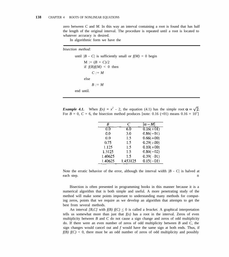
138 CHAPTER 4 ROOTS OF NONLINEAR EQUATIONS
zero between C and M. In this way an interval containing a root is found that has halfthe length of the original interval. The procedure is repeated until a root is located towhatever accuracy is desired.
In algorithmic form we have the
bisection method:
until |B - C| is sufficiently small or f(M) = 0 begin
M := (B + C)/2if f(B)f(M) < 0 then
C := M
else
B := M
end until.
Example 4.1. When f(x) = x2 - 2, the equation (4.1) has the simple rootFor B = 0, C = 6, the bisection method produces [note: 0.16 (+01) means 0.16 × 101]
Note the erratic behavior of the error, although the interval width |B - C| is halved ateach step. n
Bisection is often presented in programming books in this manner because it is anumerical algorithm that is both simple and useful. A more penetrating study of themethod will make some points important to understanding many methods for comput-ing zeros, points that we require as we develop an algorithm that attempts to get thebest from several methods.
An interval [B,C] with f(B) f(C) < 0 is called a bracket. A graphical interpretationtells us somewhat more than just that f(x) has a root in the interval. Zeros of evenmultiplicity between B and C do not cause a sign change and zeros of odd multiplicitydo. If there were an even number of zeros of odd multiplicity between B and C, thesign changes would cancel out and f would have the same sign at both ends. Thus, iff(B) f(C) < 0, there must be an odd number of zeros of odd multiplicity and possibly
4.1 BISECTION, NEWTON’S METHOD, AND THE SECANT RULE 139
some zeros of even multiplicity between B and C. If we agree to count the number ofzeros according to their multiplicity (i.e., a zero of multiplicity m counts as m zeros),then we see that there are an odd number of zeros between B and C.
A careful implementation of bisection takes into account a number of mattersraised in Chapter 1. There is a test for values off that are exactly zero; the test for achange of sign is not programmed as a test of f(B) f(C) < 0 because of the potentialfor underflow of the product; and the midpoint is computed as M = B + (B - C)/2because it is just as easy to compute and more accurate than M = (B + C)/2.
We often try to find an approximate root z for which f(z) is as small as possible.In attempting this, the finite word length of the computer must be taken into accountand so must the details of the procedure for evaluating f. Eventually even the signof the computed value may be incorrect. This is what is meant by limiting precision.Figure 1.2 shows the erratic size and sign of function values when the values are sosmall that the discrete nature of the floating point number system becomes important.If a computed function value has the wrong sign because the argument is very closeto a root, it may happen that the bracket selected in bisection does not contain a root.Even so, the approximations computed thereafter will stay in the neighborhood of theroot. It is usually said that a bisection code will produce an interval [B,C] of specifiedlength that contains a root because f(B) f(C) < 0. This is superficial. It should bequalified by saying that either this is true, or a root has been found that is as accurateas the precision allows. The qualification “as accurate as the precision allows” meanshere that either the computed f(z) vanishes, or that one of the computed values f(B),f(C) has the wrong sign.
A basic assumption of the bisection method is that f(x) is continuous. It should beno surprise that the method can fail when this is not the case. Because a bisection codepays no attention to the values of the function, it cannot tell the difference between apole of odd multiplicity and a root of odd multiplicity [unless it attempts to evaluatef(x) exactly at a pole and there is an overflow]. So, for example, if a bisection code isgiven the function tan(x) and asked to find the root in [5,7], it will have no difficulty.If asked to find the root in [4,7], it will not realize there is a root in the interval becausethe sign change due to the simple pole cancels out the sign change due to the simpleroot. And, what is worse, if asked to find a root in [4,5], it will locate a pole or causean overflow. We see here another reason for scaling: removing odd order poles byscaling removes the sign changes that might cause bisection to locate a pole ratherthan a zero. Here this is done by F(x) = cos(x) tan(x) = sin(x). One of the examplesof scaling given earlier is a less trivial illustration of the point. Because of the very realpossibility of computing a pole of odd multiplicity, it is prudent when using a bisectioncode to inspect the residual f(z) of an alleged root z-it would be highly embarrassingto claim that z results in a very small value of f(z) when it actually results in a verylarge value!
A bisection code can converge to a pole because it makes no use of the valuef(M), just its sign. Because of this its rate of convergence is the same whether the rootis simple or not and whether the function is smooth or not. Other methods convergemuch faster when the root is simple and the function is smooth, but they do not workso well when this is not the case.
Bisection has a number of virtues. Provided an initial bracket can be found, it will
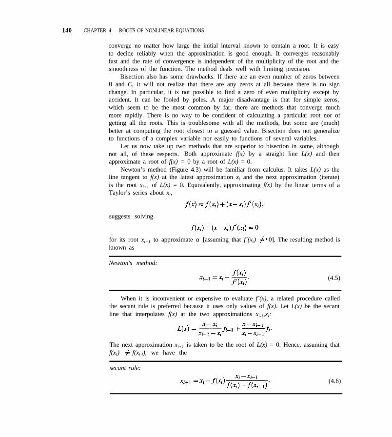
140 CHAPTER 4 ROOTS OF NONLINEAR EQUATIONS
converge no matter how large the initial interval known to contain a root. It is easyto decide reliably when the approximation is good enough. It converges reasonablyfast and the rate of convergence is independent of the multiplicity of the root and thesmoothness of the function. The method deals well with limiting precision.
Bisection also has some drawbacks. If there are an even number of zeros betweenB and C, it will not realize that there are any zeros at all because there is no signchange. In particular, it is not possible to find a zero of even multiplicity except byaccident. It can be fooled by poles. A major disadvantage is that for simple zeros,which seem to be the most common by far, there are methods that converge muchmore rapidly. There is no way to be confident of calculating a particular root nor ofgetting all the roots. This is troublesome with all the methods, but some are (much)better at computing the root closest to a guessed value. Bisection does not generalizeto functions of a complex variable nor easily to functions of several variables.
Let us now take up two methods that are superior to bisection in some, althoughnot all, of these respects. Both approximate f(x) by a straight line L(x) and thenapproximate a root of f(x) = 0 by a root of L(x) = 0.
Newton’s method (Figure 4.3) will be familiar from calculus. It takes L(x) as theline tangent to f(x) at the latest approximation xi and the next approximation (iterate)is the root xi+1 of L(x) = 0. Equivalently, approximating f(x) by the linear terms of aTaylor’s series about xi,
suggests solving
for its root xi+1 to approximate α [assuming that f´(xi) 0]. The resulting method isknown as
Newton's method:
(4.5)
When it is inconvenient or expensive to evaluate f´(x), a related procedure calledthe secant rule is preferred because it uses only values of f(x). Let L(x) be the secantline that interpolates f(x) at the two approximations xi-1,xi:
The next approximation xi+1 is taken to be the root of L(x) = 0. Hence, assuming thatf(xi) f(xi-l), we have the
secant rule:
(4.6)
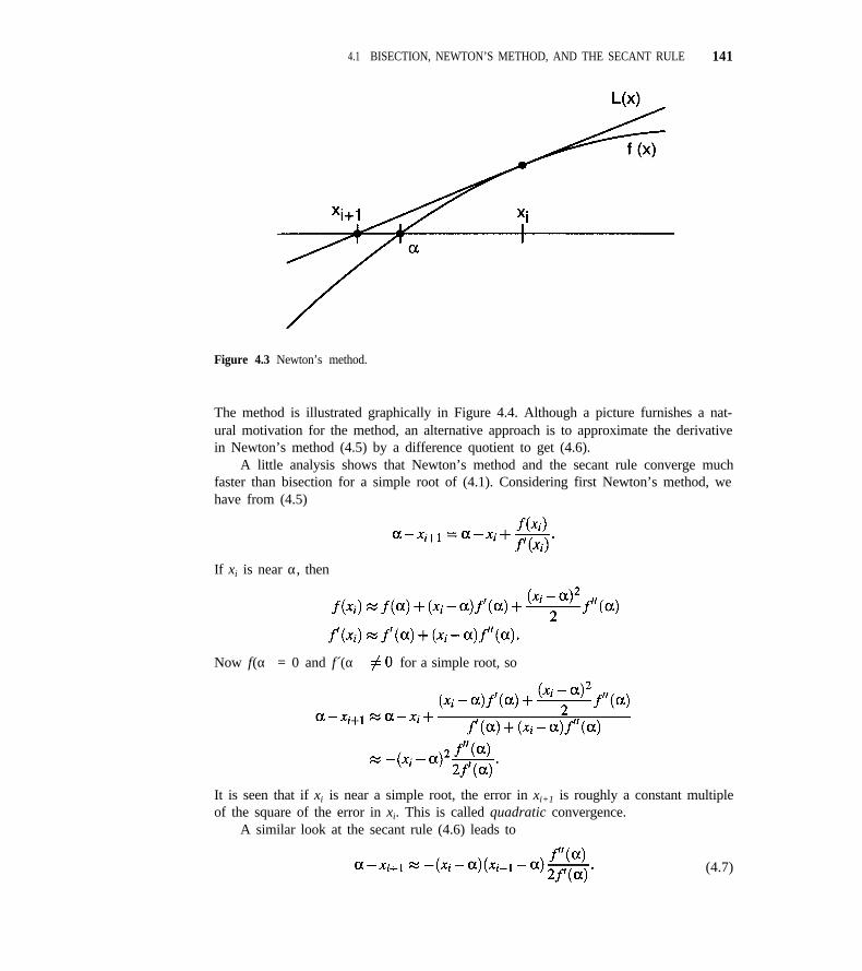
4.1 BISECTION, NEWTON’S METHOD, AND THE SECANT RULE 141
Figure 4.3 Newton’s method.
The method is illustrated graphically in Figure 4.4. Although a picture furnishes a nat-ural motivation for the method, an alternative approach is to approximate the derivativein Newton’s method (4.5) by a difference quotient to get (4.6).
A little analysis shows that Newton’s method and the secant rule converge muchfaster than bisection for a simple root of (4.1). Considering first Newton’s method, wehave from (4.5)
If xi is near α, then
Now f(α) = 0 and f´(α) for a simple root, so
It is seen that if xi is near a simple root, the error in xi+1 is roughly a constant multipleof the square of the error in xi. This is called quadratic convergence.
A similar look at the secant rule (4.6) leads to
(4.7)
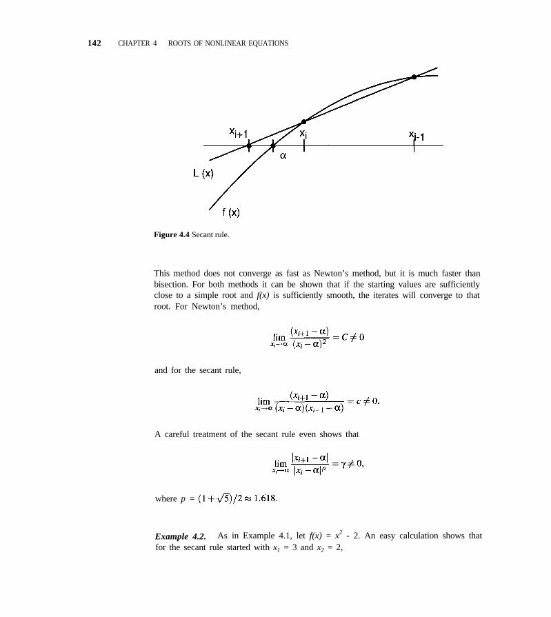
142 CHAPTER 4 ROOTS OF NONLINEAR EQUATIONS
Figure 4.4 Secant rule.
This method does not converge as fast as Newton’s method, but it is much faster thanbisection. For both methods it can be shown that if the starting values are sufficientlyclose to a simple root and f(x) is sufficiently smooth, the iterates will converge to thatroot. For Newton’s method,
and for the secant rule,
A careful treatment of the secant rule even shows that
where p =
Example 4.2. As in Example 4.1, let f(x) = x2 - 2. An easy calculation shows thatfor the secant rule started with x1 = 3 and x2 = 2,
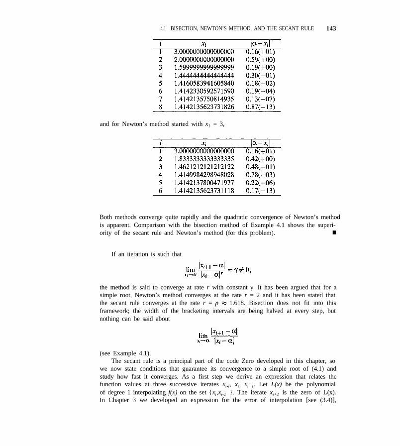
4.1 BISECTION, NEWTON’S METHOD, AND THE SECANT RULE 143
and for Newton’s method started with x1 = 3,
Both methods converge quite rapidly and the quadratic convergence of Newton’s methodis apparent. Comparison with the bisection method of Example 4.1 shows the superi-ority of the secant rule and Newton’s method (for this problem). n
If an iteration is such that
the method is said to converge at rate r with constant γ. It has been argued that for asimple root, Newton’s method converges at the rate r = 2 and it has been stated thatthe secant rule converges at the rate r = p 1.618. Bisection does not fit into thisframework; the width of the bracketing intervals are being halved at every step, butnothing can be said about
(see Example 4.1).The secant rule is a principal part of the code Zero developed in this chapter, so
we now state conditions that guarantee its convergence to a simple root of (4.1) andstudy how fast it converges. As a first step we derive an expression that relates thefunction values at three successive iterates xi-l, xi, xi+1. Let L(x) be the polynomialof degree 1 interpolating f(x) on the set {xi,xi-1 }. The iterate xi+1 is the zero of L(x).In Chapter 3 we developed an expression for the error of interpolation [see (3.4)],
144 CHAPTER 4 ROOTS OF NONLINEAR EQUATIONS
which in this case is
or, since L( xi+1) = 0,
(4.8)
for a suitable (unknown) point Some manipulation of equation (4.6) gives the tworelations
(4.9)
(4.10)
A third relation is obtained from the mean value theorem for derivatives:
(4.11)
where ζ, a point between xi and xi-l, is unknown. Combining equations (4.8)–(4.1l),we arrive at
Let us assume that on an appropriate interval we have
(4.12)
and that we are computing a simple zero a. (Why must it be simple with these hy-potheses?) Then these bounds and the expression above for f(xi+1) imply that
If we let
this inequality leads to
Supposing that
4.1 BISECTION, NEWTON’S METHOD, AND THE SECANT RULE 145
it is easy to argue by induction that
where
The formal proof is left as an exercise. Since
we see that for i large,
In any event, and since 0 < ε < 1, we must have which iswhat we wanted to prove. Let us now state a formal theorem and complete the detailsof its proof.
Theorem 4.1. The secant rule defined by (4.6) with initial guesses x0, x1 con-verges to a simple zero α of f(x) if x0, x1 lie in a sufficiently small closed intervalcontaining α on which f´(x), f´´(x) exist and are continuous and f’(x) does not van-ish.
Proof. Without loss of generality we assume that M2 defined by (4.10) is posi-tive. Otherwise f´´(x) = 0 near a, implying that f(x) is a linear function and the secantrule converges in one step. With the assumptions on f´ and f´´, the bounds m1, m2,and M2 are well defined. Using the mean value theorem for derivatives, we see that
This implies that the quantity ε defined above is less than 1 if x0 and x1 are sufficientlyclose to α. The argument above shows that
But
146 CHAPTER 4 ROOTS OF NONLINEAR EQUATIONS
Hence,
This says that The argument suggests that the rate of convergence is the goldenmean stated earlier. n
Methods that converge at a rate r > 1 are said to be superlinearly convergent. Wehave seen that this is the case for Newton’s method and the secant rule when computinga simple root. Unfortunately it is not the case when computing a multiple root. It iseasy enough to see this for Newton’s method. If xi is near a root α of multiplicitym > 1, then
This implies that
This expression shows that for a root of multiplicity m, Newton’s method is only lin-early convergent with constant (m - 1)/m.
An example from Wilkinson [11] illustrates several difficulties that can arise inthe practical application of Newton’s method.
Example 4.3. Consider the problem
x20 - l = 0.
In attempting to compute the simple root α = 1 using Newton’s method, suppose westart with x0 = 1/2. Then from (4.5)
because the tangent is nearly horizontal. Thus, a reasonably good guess for a root leadsto a much worse approximation. Also, notice that if xi is much larger than 1, then
To the same degree of approximation,
which says that we creep back to the root at 1 at a rate considerably slower thanbisection. What is happening here is that the roots of this equation are the roots of
4.1 BISECTION, NEWTON’S METHOD, AND THE SECANT RULE 147
unity. The 20 simple roots lie on a circle of radius 1 in the complex plane. The rootsare well separated, but when “seen” from as far away as 26000, they appear to form aroot of multiplicity 20, as argued earlier in this chapter. Newton’s method convergeslinearly with constant 19/20 to a root of multiplicity 20, and that is exactly what isobserved when the iterates are far from the roots.
Much is made of the quadratic convergence of Newton’s method, but it is quadrat-ically convergent only for simple roots. Even for simple roots, this example showsthat quadratic convergence is observed only when “sufficiently” close to a root. And,of course, when “too” close to a root, finite precision arithmetic affects the rate ofconvergence. n
Let us now consider the behavior of Newton’s method and the secant rule at lim-iting precision. Figure 1.2 shows an interval of machine-representable numbers aboutα on which computed values of the function vary erratically in sign and magnitude.These represent the smallest values the computed f(x) can assume when formed in theworking precision, and quite frequently they have no digits in agreement with the truef(x). For a simple root, |f´(α)| is not zero, and if the root is not ill-conditioned, thederivative is not small. As a consequence, the computed value of the first derivativeordinarily has a few digits that are correct. It then follows that the correction to xi
computed by Newton’s method is very small at limiting precision and the next iteratestays near the root even if it moves away because f(xi) has the wrong sign. This is likebisection and is what is meant by the term “stable at limiting precision.” The secantrule behaves differently. The correction to the current iterate,
has unpredictable values at limiting precision. Clearly it is possible that the next iteratelie far outside the interval of limiting precision.
There is another way to look at the secant rule that is illuminating. One approachto finding a root α of f(x) is to interpolate several values yi = f(xi) by a polyno-mial P(x) and then approximate α by a root of this polynomial. The secant rule isthe case of linear interpolation. Higher order interpolation provides a more accurateapproximation to f(x), so it is plausible that it would lead to a scheme with a higherrate of convergence. This turns out to be true, although only the increase from lin-ear to quadratic interpolation might be thought worth the trouble. The scheme basedon quadratic interpolation is called Muller’s method. Muller’s method is a little moretrouble than the secant rule, because it involves computing the roots of a quadratic, andit converges somewhat faster. There are some practical differences. For all methodsbased on interpolation by a polynomial of degree higher than 1, there is a question ofwhich root to take as the next iterate xi+1. To get convergence, the root closest to xi
should be used. An important difference between Muller’s method and the secant ruleis due to the possibility of a real quadratic polynomial having complex roots. Evenwith real iterates and a real function, Muller’s method might produce a complex iter-ate. If complex roots are interesting, this is a virtue, but if only real roots are desired,it is a defect. The secant rule can be used to compute complex roots, but it will notleave the real line spontaneously like Muller’s method. The MATHCAD documentation
148 CHAPTER 4 ROOTS OF NONLINEAR EQUATIONS
points out that its code, which is based on the secant rule, can be used to compute theroots of a complex-valued function by starting with a guess that is complex.
An alternative to direct interpolation is inverse interpolation. This approach isbased on interpolating the inverse function f--1(y) of y = f(x). To prevent confusionwith the reciprocal of f(x), the inverse function will be denoted here by G(y). Weassume that we have at our disposal only a procedure for evaluating f(x). However,each value f(xi) = yi provides a value of the inverse function because by definitionxi = G(yi). Finding a root of f(x) corresponds to evaluating the inverse function: aroot α satisfies f(α) = 0, hence α = G(0). This is a familiar task that we solve in afamiliar way. We are able to evaluate a function G(y) at certain points yi and we wishto approximate the value G(0). This is done by approximating G(y) with a polynomialinterpolant P(y) and then evaluating P(0) a. Of course, it is easy to interpolateG(y) by whatever degree polynomial we want. However, as with direct interpolation,most of the improvement to the rate of convergence is gained on going to quadraticinterpolation. An interesting fact left to an exercise is that the method derived fromlinear inverse interpolation is the same as that derived from linear direct interpolation,namely the secant rule. Examination of Figure 4.4 helps in understanding this. On theother hand, quadratic direct and inverse interpolation are quite different. For one thing,quadratic inverse interpolation cannot produce a complex iterate when the function andthe previous iterates are real.
Inverse interpolation is attractive because of its simplicity. Unfortunately, there isa fundamental difficulty—f might not have an inverse on the interval of interest. Thisis familiar from the trigonometric functions. For instance, the function y = sin(x) doesnot have an inverse for all x. To invert the relationship with x = arcsin(y) the argumentx is restricted to an interval on which sin(x) is monotone. In a plot like Figure 4.2, theinverse of f is found by “turning the picture on its side.” Only on an interval wheref(x) is monotone does the inverse function exist as a single-valued function. At asimple root a, f´(a) 0, so there is an interval containing a on whichis monotone] and G(y) exists. So, the usual kind of result is obtained. If we can startclose enough to a simple root, there is an inverse function and we can compute theroot with inverse interpolation. When some distance from a root or when the root ismultiple, there may be serious difficulties with inverse interpolation because then thefunction does not have an inverse on the relevant interval.
With the exception of bisection, the methods we have studied are guaranteed toconverge only when sufficiently close to a zero of a function that is sufficiently smooth.This is rather unsatisfactory when we have no idea about where the roots are. On theother hand, often we are interested in the root closest to a specific value. It is by nomeans certain that the methods will converge from this value to the nearest root sincethat depends on just how close the value is to the root, but it is a useful characteristic ofthe methods. In contrast, if the initial bracket given a bisection code contains severalroots, the code might locate any one of them. The technique of continuation is usefulwhen it is hard to find a starting guess good enough to get convergence to a particularroot, or to any root. Many problems depend on a parameter λ and it may be that zeroscan be computed easily for some values of the parameter. The family x exp(-x) - γ = 0is an example. Solutions are desired for values γ > 0, but it is obvious that a = 0is a root when γ = 0. It is generally the case, although not always, that the roots
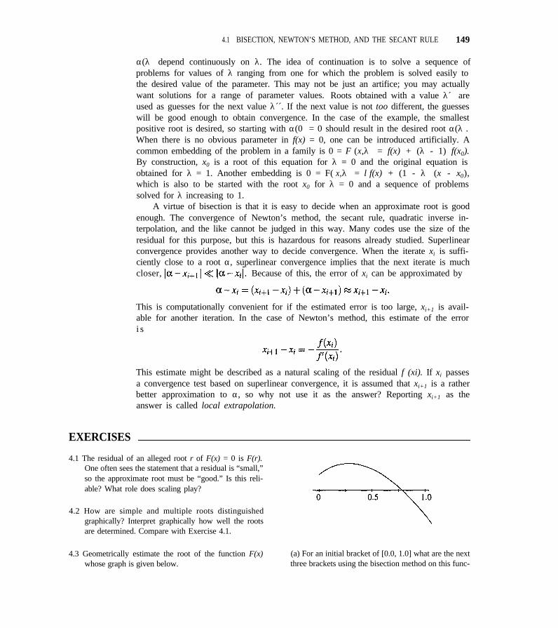
4.1 BISECTION, NEWTON’S METHOD, AND THE SECANT RULE 149
α(λ) depend continuously on λ. The idea of continuation is to solve a sequence ofproblems for values of λ ranging from one for which the problem is solved easily tothe desired value of the parameter. This may not be just an artifice; you may actuallywant solutions for a range of parameter values. Roots obtained with a value λ ́ areused as guesses for the next value λ´´. If the next value is not too different, the guesseswill be good enough to obtain convergence. In the case of the example, the smallestpositive root is desired, so starting with α(0) = 0 should result in the desired root α(λ).When there is no obvious parameter in f(x) = 0, one can be introduced artificially. Acommon embedding of the problem in a family is 0 = F (x,λ) = f(x) + (λ - 1) f(x0).By construction, x0 is a root of this equation for λ = 0 and the original equation isobtained for λ = 1. Another embedding is 0 = F( x,λ) = λf(x) + (1 - λ) (x - x0),which is also to be started with the root x0 for λ = 0 and a sequence of problemssolved for λ increasing to 1.
A virtue of bisection is that it is easy to decide when an approximate root is goodenough. The convergence of Newton’s method, the secant rule, quadratic inverse in-terpolation, and the like cannot be judged in this way. Many codes use the size of theresidual for this purpose, but this is hazardous for reasons already studied. Superlinearconvergence provides another way to decide convergence. When the iterate xi is suffi-ciently close to a root α, superlinear convergence implies that the next iterate is muchcloser, Because of this, the error of xi can be approximated by
This is computationally convenient for if the estimated error is too large, xi+1 is avail-able for another iteration. In the case of Newton’s method, this estimate of the errori s
This estimate might be described as a natural scaling of the residual f (xi). If xi passesa convergence test based on superlinear convergence, it is assumed that xi+1 is a ratherbetter approximation to α, so why not use it as the answer? Reporting xi+1 as theanswer is called local extrapolation.
EXERCISES
4.1 The residual of an alleged root r of F(x) = 0 is F(r).One often sees the statement that a residual is “small,”so the approximate root must be “good.” Is this reli-able? What role does scaling play?
4.2 How are simple and multiple roots distinguishedgraphically? Interpret graphically how well the rootsare determined. Compare with Exercise 4.1.
4.3 Geometrically estimate the root of the function F(x) (a) For an initial bracket of [0.0, 1.0] what are the nextwhose graph is given below. three brackets using the bisection method on this func-
150 CHAPTER 4 ROOTS OF NONLINEAR EQUATIONS
tion? linear polynomial that interpolates G(y) at f(xi) and
(b) If xl = 0.0 and x2 = 1.0, mark on the graph the f(xi-l), show that P(0) = xi+1 is given by (4.6).
approximate location of x3 using one step of the se- 4.7 In the convergence proof for the secant rule, it wascant method. stated that if ε = max(ε0, ε1) < 1, then the inequality
(c) If x1 = 0.5, mark on the graph the approximatelocation of x2 and x3 using two steps of Newton’smethod.
4.4 The polynomial f(x) = x3 - 2x - 5 has a root a in[2,3].
(a) Show that [2,3] is a bracket for f(x).
(b) Apply four steps of the bisection method to re-duce the width of the bracket to 1/16.
(c) Calculate x3 and x4 by the secant method startingwith xl = 3 and x2 = 2.
(d) Calculate x2, x3, and x4 using Newton’s methodwith x1 = 2.
4.5 To find where sinx = x/2 for x > 0,
(a) find a bracket for an appropriate function f(x).
(b) Apply four steps of the bisection method to re-duce the width of the bracket by 1/16.
(c) Calculate x3 and x4 by the secant method startingwith x1 and x2 equal to the bracket values.
(d) Calculate x2, x3, and x4 using Newton’s methodwith x1 the midpoint of your bracket.
4.6 Given x0 and x1, show that the inverse secant rule,discussed at the end of Section 4.1, and the direct se-cant rule (4.6) produce the same iterates. In particular,with G(y) the inverse function of f(x), and P(y) the
implied
and
Establish this.
4.8 The special function
is important in statistics and in many areas of scienceand engineering. Because the integrand is positive forall t, the function is strictly increasing and so has aninverse x = erf-1(y). The inverse error function is animportant function in its own right and can be evalu-ated for given y by solving the equation y = erf(x).The algorithm of the MATLAB function erfinv.mfirst forms a rational approximation to y that is ac-curate to about six figures. Two Newton iterationsare then done to get a result to full accuracy. Whatis Newton’s method for solving this equation? Whywould you expect two iterations to be enough? (Don’tforget to consider the multiplicity of the root.)
4.2 AN ALGORITHM COMBINING BISECTION AND THE SECANT RULE
It is a challenging task to fuse several methods into an efficient computational scheme.This section is devoted to a code, Zero, based on one written by Dekker [6] that doesthis. Roughly speaking, the code uses the secant rule unless bisection appears advan-tageous. A very similar code is found in the NAG library. Brent [3] added the use ofquadratic inverse interpolation to Dekker’s ideas. Brent’s code is the basis for codes inMATLAB and the IMSL library.
Normal input to Zero is a subprogram for the evaluation of a continuous functionf(x) and arguments B and C for which f(B)f(C) < 0. Throughout the computationB and C are end points of an interval with f(B)f(C) < 0 that is decreasing in length.In favorable circumstances B is computed with the secant rule and is a much betterapproximate root than either C or the midpoint M = (C + B)/2 of the interval. To
4.2 AN ALGORITHM COMBINING BISECTION AND THE SECANT RULE 151
deal with unfavorable circumstances, the code interchanges the values of B and C asnecessary so that |f(B)| < |f(C)| holds. If at any time the computed f(B) is zero, thecomputation is terminated and B is reported as a root.
The convergence test is a mixed relative-absolute error test. Two parameters AB-SERR and RELERR are input and it is asked of each iterate whether
(4.13)
For reasons discussed in Chapter 1, the code will not permit RELERR to be smallerthan 10 units of roundoff, nor ABSERR to be zero. However, to understand what thetest means, first suppose that RELERR is zero. The test is then asking if an intervalbelieved to contain a root has a length no more than 2 × ABSERR. If so, the midpointM is no farther than ABSERR from a root and this is a pure absolute error test onM as an approximate root. However, it is believed that the quantity B reported as theanswer is closer to a root than M is. Even if it is not, the test implies that B is within2 × ABSERR of a root. Similarly, if the parameter ABSERR is zero and if the testwere
the test would be a pure relative error test for the approximate root M. Because it isbelieved that B is a better approximate root, it is used in the test rather than M. Thefzero.m function in MATLAB has a similar, but somewhat simpler, test. The codes inthe NAG and lMSL libraries have convergence tests that are broadly similar, but theyalso test the size of the residual and convergence can occur either because the root hasbeen located to a specified accuracy or because the magnitude of the residual is smallerthan a specified value.
Unless there is a reason to do otherwise, Zero uses the secant rule. A variable A isinitialized to C. The two variables A, B are the two iterates used by the secant rule tocalculate
A danger with the secant rule (and Newton’s method) is an interpolant that is horizontalor nearly so. The extreme case is a division by zero in this formula. This danger isavoided by requiring D to lie in the interval [B,C] known to contain a root and checkingthis without performing the division. Pursuing the tactic further, the code requires thatD lie in [B,M] on the grounds that B ought to be a better approximation to the root thanC, so if the secant rule is working properly, D ought to be closer to B than to C. If Ddoes not lie in [B,M], the midpoint M is used as the next iterate.
The performance of the code can be improved in some circumstances by selectingan iterate in a different way. If D is too close to B, a better tactic is to move a minimumdistance away from B. The quantity max[ABSERR, |B| × RELERR] is called TOL inthe code. If |D - B| < TOL, then the value B + TOL × sign(C - B) is used instead ofD. This choice cannot result in an iterate outside the interval [B,C] since |B - C| >2 × TOL (or else the error test would have been passed). If the root a is further from
152 CHAPTER 4 ROOTS OF NONLINEAR EQUATIONS
B than TOL, the iterate chosen in this way is closer to the root than D. If it is closer,this iterate and B will bracket the root and the code will converge at the next test onthe error because the length of the bracket is TOL.
There are circumstances in which the current iterate B is converging to a root, butthe end point C is fixed. Because convergence is judged by the length of the interval[B,C] and because the rate of convergence of the secant rule depends on using valuesfrom the neighborhood of the root, the code monitors the length of the interval. If fouriterations have not resulted in a reduction by a factor of l/8, the code bisects threetimes. This guarantees that the code will reduce the length of an interval containing aroot by a factor of l/8 in a maximum of seven function evaluations.
In summary, if the value D of the secant rule lies outside [B,M] or if the overallreduction in interval length has been unsatisfactory, the code bisects the interval. IfD is too close to B, a minimum change of TOL is used. Otherwise D is used. Afterdeciding how to compute the next iterate, it is formed explicitly and replaces B. Iff(B) = 0, the code exits. Otherwise, quantities are updated for the next iteration: theold B replaces A. The old C is kept or is replaced by the old B, whichever results in
f(B)f(C) < 0.If the code is given normal input [f(x) continuous, f(B)f(C) < 01, then on nor-
mal return, either the computed f(B) = 0, or the computed f(B) and f(C) satisfyf(B)f(C) < 0, |f(B)| < |f(C)| and the output values of B and C satisfy (4.13). Inthe latter case there is either a root of f(x) in the interval [B,C] or else one of the endpoints is so close to a root that the sign has been computed incorrectly in the workingprecision.
EXERCISES
4.9 The algorithm described combining the bisectionmethod with the secant method is very efficient. Sup-pose that the initial B and C satisfy |B - C| = 1010,and a root is sought with an absolute error of at most1 0 - 5
(a) How many function evaluations does the bisec-tion method use?
(b) What is the maximum number of function evalu-ations needed by the combined algorithm?
4.3 ROUTINES FOR ZERO FINDING
The algorithm of the preceding section has been implemented in a routine called Zerodesigned to compute a root of the nonlinear equation F(x) = 0. A typical invocationof Zero in C++ is
flag = Zero(f, b, c, abserr, relerr, residual);
in FORTRAN it is
CALL ZERO(F, B, C, ABSERR, RELERR, RESIDL, FLAG)
and
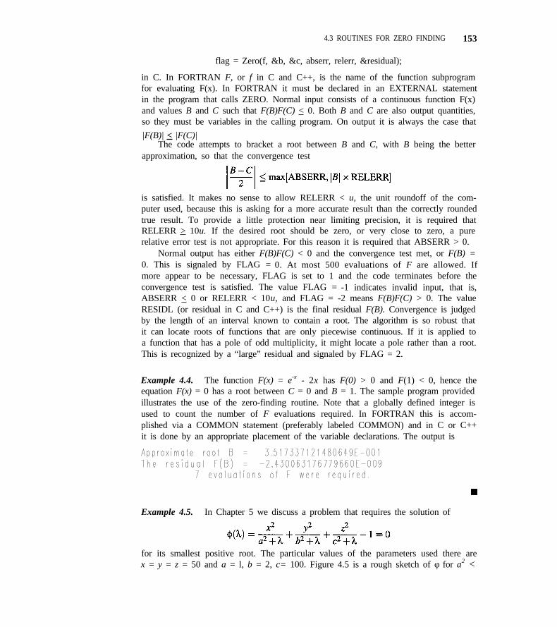
4.3 ROUTINES FOR ZERO FINDING 153
flag = Zero(f, &b, &c, abserr, relerr, &residual);
in C. In FORTRAN F, or f in C and C++, is the name of the function subprogramfor evaluating F(x). In FORTRAN it must be declared in an EXTERNAL statementin the program that calls ZERO. Normal input consists of a continuous function F(x)and values B and C such that F(B)F(C) < 0. Both B and C are also output quantities,so they must be variables in the calling program. On output it is always the case that
|F(B)| < |F(C)|The code attempts to bracket a root between B and C, with B being the better
approximation, so that the convergence test
is satisfied. It makes no sense to allow RELERR < u, the unit roundoff of the com-puter used, because this is asking for a more accurate result than the correctly roundedtrue result. To provide a little protection near limiting precision, it is required thatRELERR > 10u. If the desired root should be zero, or very close to zero, a purerelative error test is not appropriate. For this reason it is required that ABSERR > 0.
Normal output has either F(B)F(C) < 0 and the convergence test met, or F(B) =0. This is signaled by FLAG = 0. At most 500 evaluations of F are allowed. Ifmore appear to be necessary, FLAG is set to 1 and the code terminates before theconvergence test is satisfied. The value FLAG = -1 indicates invalid input, that is,ABSERR < 0 or RELERR < 10u, and FLAG = -2 means F(B)F(C) > 0. The valueRESIDL (or residual in C and C++) is the final residual F(B). Convergence is judgedby the length of an interval known to contain a root. The algorithm is so robust thatit can locate roots of functions that are only piecewise continuous. If it is applied toa function that has a pole of odd multiplicity, it might locate a pole rather than a root.This is recognized by a “large” residual and signaled by FLAG = 2.
Example 4.4. The function F(x) = e-x - 2x has F(0) > 0 and F(1) < 0, hence theequation F(x) = 0 has a root between C = 0 and B = 1. The sample program providedillustrates the use of the zero-finding routine. Note that a globally defined integer isused to count the number of F evaluations required. In FORTRAN this is accom-plished via a COMMON statement (preferably labeled COMMON) and in C or C++it is done by an appropriate placement of the variable declarations. The output is
Example 4.5. In Chapter 5 we discuss a problem that requires the solution of
for its smallest positive root. The particular values of the parameters used there arex = y = z = 50 and a = l, b = 2, c= 100. Figure 4.5 is a rough sketch of φ for a2 <
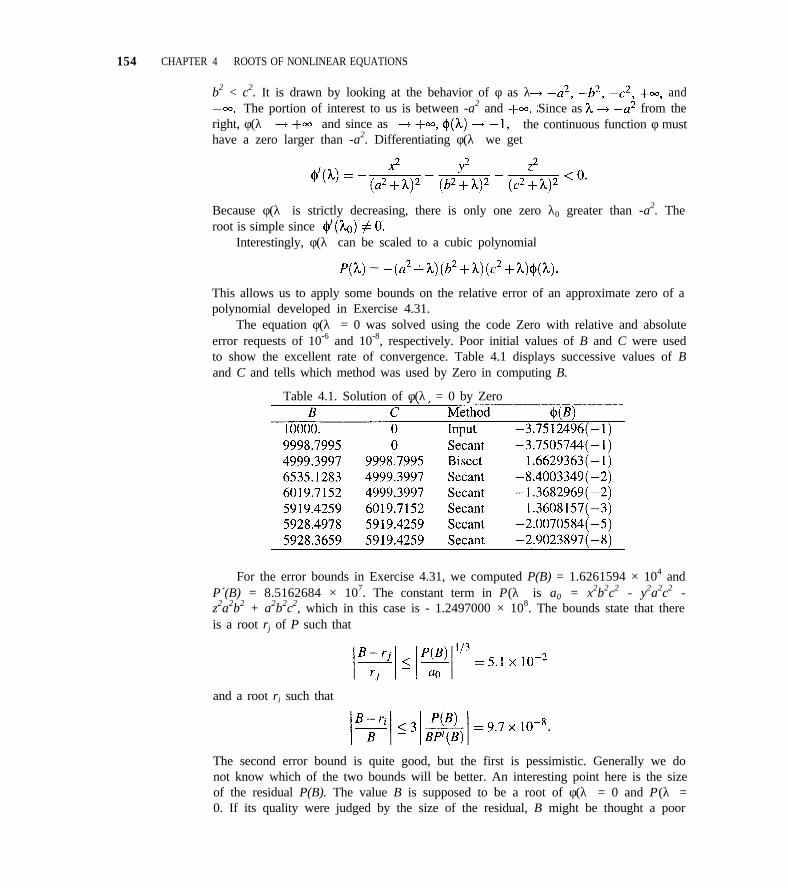
154 CHAPTER 4 ROOTS OF NONLINEAR EQUATIONS
b2 < c2. It is drawn by looking at the behavior of φ as λ andThe portion of interest to us is between -a2 and Since as from the
right, φ(λ) and since as the continuous function φ musthave a zero larger than -a2. Differentiating φ(λ) we get
Because φ(λ) is strictly decreasing, there is only one zero λ0 greater than -a2. Theroot is simple since
Interestingly, φ(λ) can be scaled to a cubic polynomial
This allows us to apply some bounds on the relative error of an approximate zero of apolynomial developed in Exercise 4.31.
The equation φ(λ) = 0 was solved using the code Zero with relative and absoluteerror requests of 10-6 and 10-8, respectively. Poor initial values of B and C were usedto show the excellent rate of convergence. Table 4.1 displays successive values of Band C and tells which method was used by Zero in computing B.
Table 4.1. Solution of φ(λ) = 0 by Zero
For the error bounds in Exercise 4.31, we computed P(B) = 1.6261594 × 10⁴ andP´(B) = 8.5162684 × 10⁷. The constant term in P(λ) is a0 = x2b2c2 - y2a2c2 -z2a2b2 + a2b2c2, which in this case is - 1.2497000 × 10⁸. The bounds state that thereis a root rj of P such that
and a root ri such that
The second error bound is quite good, but the first is pessimistic. Generally we donot know which of the two bounds will be better. An interesting point here is the sizeof the residual P(B). The value B is supposed to be a root of φ(λ) = 0 and P(λ) =0. If its quality were judged by the size of the residual, B might be thought a poor
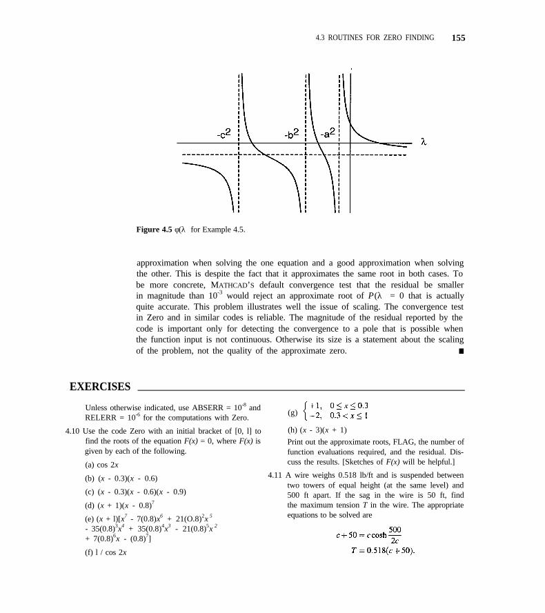
4.3 ROUTINES FOR ZERO FINDING 155
Figure 4.5 φ(λ) for Example 4.5.
approximation when solving the one equation and a good approximation when solvingthe other. This is despite the fact that it approximates the same root in both cases. Tobe more concrete, MATHCAD’S default convergence test that the residual be smallerin magnitude than 10-3 would reject an approximate root of P(λ) = 0 that is actuallyquite accurate. This problem illustrates well the issue of scaling. The convergence testin Zero and in similar codes is reliable. The magnitude of the residual reported by thecode is important only for detecting the convergence to a pole that is possible whenthe function input is not continuous. Otherwise its size is a statement about the scalingof the problem, not the quality of the approximate zero. n
EXERCISES
Unless otherwise indicated, use ABSERR = 10-8 and(g)
RELERR = 10-6 for the computations with Zero.
4.10 Use the code Zero with an initial bracket of [0, l] to (h) (x - 3)(x + 1)find the roots of the equation F(x) = 0, where F(x) is Print out the approximate roots, FLAG, the number ofgiven by each of the following. function evaluations required, and the residual. Dis-
(a) cos 2x cuss the results. [Sketches of F(x) will be helpful.]
(b) (x - 0.3)(x - 0.6) 4.11 A wire weighs 0.518 lb/ft and is suspended between
(c) (x - 0.3)(x - 0.6)(x - 0.9)two towers of equal height (at the same level) and500 ft apart. If the sag in the wire is 50 ft, find
(d) (x + 1)(x - 0.8)7
(e) (x + l)[x7 - 7(0.8)x6 + 21(O.8)2x 5
- 35(0.8)3x4 + 35(0.8)4x3 - 21(0.8)5x 2
+ 7(0.8)6x - (0.8)7]
(f) l / cos 2x
the maximum tension T in the wire. The appropriateequations to be solved are
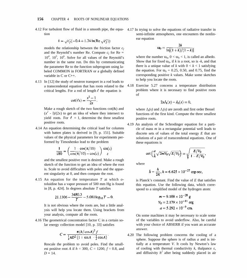
156 CHAPTER 4 ROOTS OF NONLINEAR EQUATIONS
4.12 For turbulent flow of fluid in a smooth pipe, the equa- 4.17 In trying to solve the equations of radiative transfer intion semi-infinite atmospheres, one encounters the nonlin-
ear equation
models the relationship between the friction factor cf
and the Reynold’s number Re. Compute cf for Re =104, 105, 106. Solve for all values of the Reynold’s where the number ω0, 0 < ω0 < 1, is called an albedo.
number in the same run. Do this by communicating Show that for fixed ω0, if k is a root, so is -k, and that
the parameter Re to the function subprogram using la- there is a unique value of k with 0 < k < 1 satisfying
beled COMMON in FORTRAN or a globally defined the equation. For ω0 = 0.25, 0.50, and 0.75, find the
variable in C or C++. corresponding positive k values. Make some sketches
4.13 In [12] the study of neutron transport in a rod leads toto help you locate the roots.
a transcendental equation that has roots related to the 4.18 Exercise 5.27 concerns a temperature distribution
critical lengths. For a rod of length the equation is problem where it is necessary to find positive rootsof
Make a rough sketch of the two functions cot(&) and(x2 - l)/(2x) to get an idea of where they intersect toyield roots. For = 1, determine the three smallestpositive roots.
4.14 An equation determining the critical load for columnswith batten plates is derived in [9, p. 151]. Suitablevalues of the physical parameters for experiments per-formed by Timoshenko lead to the problem
and the smallest positive root is desired. Make a roughsketch of the function to get an idea of where the rootis. Scale to avoid difficulties with poles and the appar-ent singularity at 0, and then compute the root.
4.15 An equation for the temperature T at which o-toluidine has a vapor pressure of 500 mm Hg is foundin [8, p. 424]. In degrees absolute T satisfies
It is not obvious where the roots are, but a little anal-ysis will help you locate them. Using brackets fromyour analysis, compute all the roots.
4.16 The geometrical concentration factor C in a certain so-lar energy collection model [10, p. 33] satisfies
Rescale the problem to avoid poles. Find the small-est positive root A if h = 300, C = 1200, f = 0.8, andD = 14.
where J0(x) and J1(x) are zeroth and first order Bessel functions of the first kind. Compute the three smallestpositive roots.
4.19 An analysis of the Schrodinger equation for a parti-cle of mass m in a rectangular potential well leads todiscrete sets of values of the total energy E that aresolutions of a pair of transcendental equations. One ofthese equations is
where
is Planck’s constant. Find the value of E that satisfiesthis equation. Use the following data, which corre-spond to a simplified model of the hydrogen atom:
On some machines it may be necessary to scale someof the variables to avoid underflow. Also, be carefulwith your choice of ABSERR if you want an accurateanswer.
4.20 The following problem concerns the cooling of asphere. Suppose the sphere is of radius a and is ini-tially at a temperature V. It cools by Newton’s lawof cooling with thermal conductivity k, thalpance ε,and diffusivity h2 after being suddenly placed in air
4.4 CONDITION, LIMITING PRECISION, AND MULTIPLE ROOTS 157
at 0°C. It can be shown that the temperature θ(r,t) attime t > 0 and radius r is
Here the γn are the (positive) roots of
and
For a steel sphere cooling in air at 0°C, suppose theinitial temperature is V = 100°C and the radius isa = 0.30 meters. Appropriate physical constants areh2 = 1.73 × 10⁻⁵, ε = 20, and k = 60. Find the threesmallest values of γna and use them to compute A1,A2, and A3. Approximate the temperature at r = 0.25for t = 10k seconds, k = 2, 3, 4, 5.
4.21 When solving f(x) = 0, the subroutine Zero requiresyou to input B and C such that f(B)f(C) < 0. Oftenit is not obvious what to use for B and C, so manyroutines that are similar to Zero begin with a search
for B and C that provide a change of sign. Write aroutine Root that first finds a change of sign and thencalls Zero to compute a root. The parameter list ofRoot should be the same as that of Zero except thatB and C are replaced by arguments Z and SCALE.Here the Z input is a guess for a root. If all goes well,on output Z is to be the answer B obtained by Zero.The search algorithm you are to implement is essen-tially that of the fzero.m program of MATLAB. How-ever, fzero.m begins searching with an incrementZ/20 if Z 0 and 1/20 otherwise. In Root the initialsearch increment is to be an input variable SCALE.Initialize DZ = SCALE, B = Z - DZ, C = Z + DZ.If f(B)f(C) < 0 (be sure to code this properly), callZero to compute a root. Otherwise, double the incre-ment, DZ = 2 × DZ, expand the search to the left byB = B - DZ, and test again. If this does not result ina change of sign, expand the search to the right byC = C + DZ and test again. If this does not resultin a change of sign, double the increment and repeat.Limit the number of tries. Test your code using one ofthe examples in the text. After you are sure it works,you might want to use it in other exercises.
4.4 CONDITION, LIMITING PRECISION, AND MULTIPLE ROOTS
It is important to ask what limitations on accuracy are imposed by finite precisionarithmetic. Since we seek a machine representable number that makes as nearlyzero as possible, the details of the computation off, the machine word length, and theroundoff characteristics play important roles. We have remarked that the computedfunction values may vary erratically in an interval about the zero and we have seen anexample in Figure 1.2. Let us look at another example in more detail.
Example 4.6. Consider the polynomial (x - 1)3 that we evaluate in the form ((x -3) x + 3)x - 1 in three-digit decimal chopped floating point arithmetic. For x = 1.00, 1.01,. . ., 1.17 the computed function values are exactly zero with the exception of the value0.0100 at x = 1.01, 1.11, 1.15. For x = 1.18, 1.19,. . . ,1.24 all function values are0.200 except for a value of exactly zero at x = 1.20 and a value of 0.0200 at x = 1.23.The reader might enjoy evaluating the function for x values less than 1 to explore thisphenomenon. It is clear that these erratic values might cause the secant rule to be un-stable. Evaluating the derivative shows that Newton’s method can also be unstable ata multiple root like this one. n
What effect on the accuracy of a root does inaccuracy in the function values have?To get some feeling for this, suppose that the routine for f(x) actually returns a value
158 CHAPTER 4 ROOTS OF NONLINEAR EQUATIONS
and for x a machine number near a root a, the best we can say is that
for a suitable e. Suppose that z is a machine number and = 0. How much in errorcan z be? If a is of multiplicity m, then
Since it is possible for f(z) to be as large as e, we could have
so it is possible that
(4.14)
For small ε and m > 1 the term ε1 / m is much larger than ε and there is a serious loss ofaccuracy. The other factor plays a role, but generally we must consider multiple rootsto be ill-conditioned (sensitive to errors in the evaluation off). The ill conditioning ofthe root of multiplicity 3 in (x - 1)3 = 0 is evident in Example 4.6. We saw there thatx = 1.20 led to a function value of exactly zero, and this is certainly a poor approxi-mation to the root at 1.00. The essence of the matter is that at a multiple root, f(x)is almost tangent to the horizontal axis so that shifting the curve vertically by a smallamount shifts its intersection with the axis by a considerable amount. Exercise 4.24 isan example of this effect.
Even when m = 1, the root can be poorly determined. As we have already seen,clusters of roots “look” like multiple roots from a distance, but we are now consideringwhat happens close to a root. Even when well separated and simple, a root is poorlydetermined if f(x) passes through zero with a small slope. More formally, the quantity
can be large when the slope |f´ (α)| is small. A famous example from Wilkinson [11,p. 43] illustrates this dramatically.
Example 4.7. Consider the polynomial equation
(x - 1)(x - 2)···(x - 19)(x - 20) = 0,
which has the roots 1, 2,. . . , 19, 20. These roots are obviously simple and well sepa-rated. The coefficient of xl9 is -210. If this coefficient is changed by 2-23 to become-210.000000119, the roots become those shown in Table 4.2.
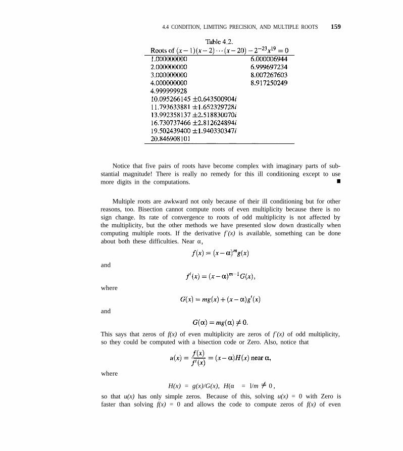
4.4 CONDITION, LIMITING PRECISION, AND MULTIPLE ROOTS 159
Notice that five pairs of roots have become complex with imaginary parts of sub-stantial magnitude! There is really no remedy for this ill conditioning except to usemore digits in the computations. n
Multiple roots are awkward not only because of their ill conditioning but for otherreasons, too. Bisection cannot compute roots of even multiplicity because there is nosign change. Its rate of convergence to roots of odd multiplicity is not affected bythe multiplicity, but the other methods we have presented slow down drastically whencomputing multiple roots. If the derivative f´(x) is available, something can be doneabout both these difficulties. Near α,
and
where
and
This says that zeros of f(x) of even multiplicity are zeros of f´(x) of odd multiplicity,so they could be computed with a bisection code or Zero. Also, notice that
where
H(x) = g(x)/G(x), H(α) = l/m 0 ,
so that u(x) has only simple zeros. Because of this, solving u(x) = 0 with Zero isfaster than solving f(x) = 0 and allows the code to compute zeros of f(x) of even
160 CHAPTER 4 ROOTS OF NONLINEAR EQUATIONS
multiplicity. However, it must be appreciated that u(x) has a pole wherever f(x) = 0and f(x) 0.
EXERCISES
4.22 What is the value of the right-hand side of (4.14) for for the condition of this root. Perturb f(x) by 10-7
the root in Exercise 4.10a? using the form in Exercise 4.10e; then solve
4.23 What is the value of the right-hand side of (4.14) for f(x) + 10-7 = 0the root of f(x) = (x- 10)(3x- 1)2 in [0,l]? Assumethat ε = 10-12.
accurately with Zero (use ABSERR = RELERR =10-10). How much was the root 0.8 perturbed? Com-
4.24 The problem f(x) = (x + 1)(x - 0.8)7 = 0 has 0.8 as a pare this to the result of (4.14) with ε = 10-7. Repeatroot of multiplicity 7. Evaluate the expression (4.14) using the form in Exercise 4.10d.
4.5 NONLINEAR SYSTEMS OF EQUATIONS
A problem occurring quite frequently in computational mathematics is to find some orall of the solutions of a system of n simultaneous nonlinear equations in n unknowns.Such problems are generally much more difficult than a single equation. An obviousstarting point is to generalize the methods we have studied for the case n = 1. Unfor-tunately, the bracketing property of the method of bisection does not hold for n > 1.There is a generalization of the secant method, but it is not at all obvious because of themore complicated geometry in higher dimensions. Newton’s method, however, doesextend nicely. Only the case n = 2 is examined because the notation is simpler and thebasic ideas are the same for the general case.
Consider the system of equations
f(x,y) = 0
g(x,y) = 0,
(4.15)
which we occasionally write in vector form as
To solve (4.15), Newton’s method for finding the root of a single nonlinear equa-tion is generalized to two dimensions. The functions f(x,y) and g(x,y) are expandedabout a point (x0, y0) using Taylor’s theorem for functions of two variables (see the ap-pendix for a statement of the theorem). Carrying only terms of degrees 0 and 1 givesthe approximating system
(4.16)
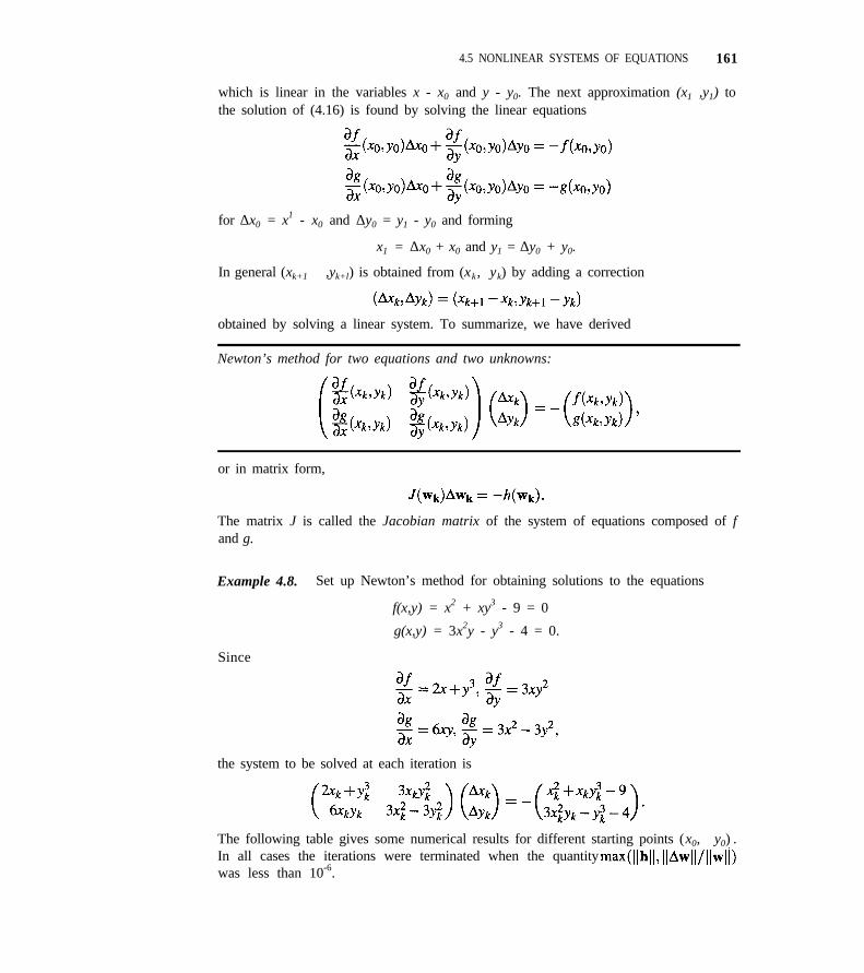
4.5 NONLINEAR SYSTEMS OF EQUATIONS 161
which is linear in the variables x - x0 and y - y0. The next approximation (x1 ,y1) tothe solution of (4.16) is found by solving the linear equations
for ∆x0 = x1 - x0 and ∆y0 = y1 - y0 and forming
x1 = ∆x0 + x0 and y1 = ∆y0 + y0.
In general (xk+1 ,yk+l) is obtained from (xk, yk) by adding a correction
obtained by solving a linear system. To summarize, we have derived
Newton’s method for two equations and two unknowns:
or in matrix form,
The matrix J is called the Jacobian matrix of the system of equations composed of fand g.
Example 4.8. Set up Newton’s method for obtaining solutions to the equations
f(x,y) = x2 + xy3 - 9 = 0
g(x,y) = 3x2y - y3 - 4 = 0.
Since
the system to be solved at each iteration is
The following table gives some numerical results for different starting points (x0, y0) .In all cases the iterations were terminated when the quantitywas less than 10-6.
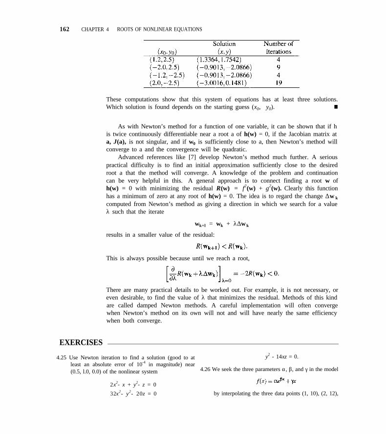
162 CHAPTER 4 ROOTS OF NONLINEAR EQUATIONS
These computations show that this system of equations has at least three solutions.Which solution is found depends on the starting guess (x0, y0). n
As with Newton’s method for a function of one variable, it can be shown that if his twice continuously differentiable near a root a of h(w) = 0, if the Jacobian matrix ata, J(a), is not singular, and if w0 is sufficiently close to a, then Newton’s method willconverge to a and the convergence will be quadratic.
Advanced references like [7] develop Newton’s method much further. A seriouspractical difficulty is to find an initial approximation sufficiently close to the desiredroot a that the method will converge. A knowledge of the problem and continuationcan be very helpful in this. A general approach is to connect finding a root w ofh(w) = 0 with minimizing the residual R(w) = f2(w) + g2(w). Clearly this functionhas a minimum of zero at any root of h(w) = 0. The idea is to regard the change ∆w k
computed from Newton’s method as giving a direction in which we search for a valueλ such that the iterate
wk+l = wk + λ∆w k
results in a smaller value of the residual:
This is always possible because until we reach a root,
There are many practical details to be worked out. For example, it is not necessary, oreven desirable, to find the value of λ that minimizes the residual. Methods of this kindare called damped Newton methods. A careful implementation will often convergewhen Newton’s method on its own will not and will have nearly the same efficiencywhen both converge.
EXERCISES
4.25 Use Newton iteration to find a solution (good to at y2 - 14xz = 0.least an absolute error of 10-4 in magnitude) near(0.5, l.0, 0.0) of the nonlinear system 4.26 We seek the three parameters α, β, and γ in the model
2x2- x + y2- z = 0
32x2- y2- 20z = 0 by interpolating the three data points (1, 10), (2, 12),
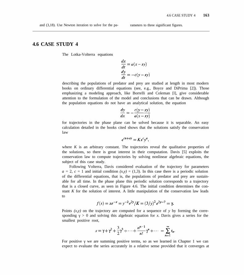
and (3,18). Use Newton iteration to solve for the pa-
4.6 CASE STUDY 4
rameters to three significant figures.
163
4.6 CASE STUDY 4
The Lotka-Volterra equations
describing the populations of predator and prey are studied at length in most modernbooks on ordinary differential equations (see, e.g., Boyce and DiPrima [2]). Thoseemphasizing a modeling approach, like Borrelli and Coleman [l], give considerableattention to the formulation of the model and conclusions that can be drawn. Althoughthe population equations do not have an analytical solution, the equation
for trajectories in the phase plane can be solved because it is separable. An easycalculation detailed in the books cited shows that the solutions satisfy the conservationlaw
where K is an arbitrary constant. The trajectories reveal the qualitative properties ofthe solutions, so there is great interest in their computation. Davis [5] exploits theconservation law to compute trajectories by solving nonlinear algebraic equations, thesubject of this case study.
Following Volterra, Davis considered evaluation of the trajectory for parametersa = 2, c = 1 and initial condition (x,y) = (1,3). In this case there is a periodic solutionof the differential equations, that is, the populations of predator and prey are sustain-able for all time. In the phase plane this periodic solution corresponds to a trajectorythat is a closed curve, as seen in Figure 4.6. The initial condition determines the con-stant K for the solution of interest. A little manipulation of the conservation law leadsto
Points (x,y) on the trajectory are computed for a sequence of y by forming the corre-sponding γ > 0 and solving this algebraic equation for x. Davis gives a series for thesmallest positive root,
For positive γ we are summing positive terms, so as we learned in Chapter 1 we canexpect to evaluate the series accurately in a relative sense provided that it converges at
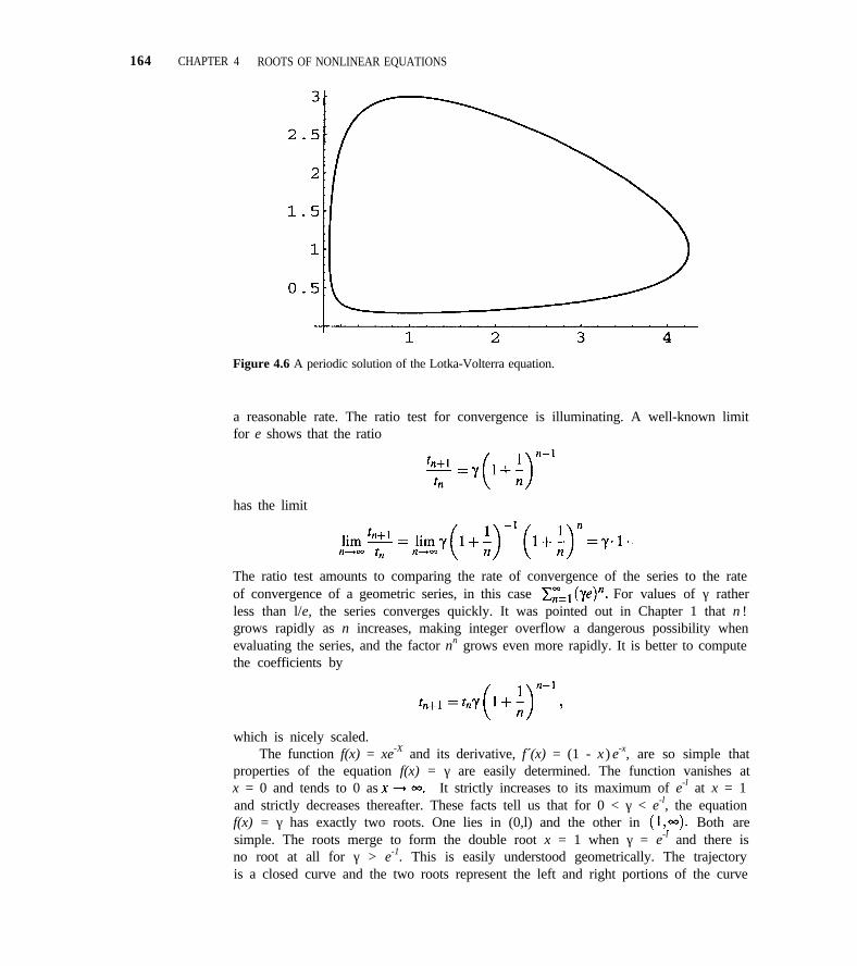
164 CHAPTER 4 ROOTS OF NONLINEAR EQUATIONS
Figure 4.6 A periodic solution of the Lotka-Volterra equation.
a reasonable rate. The ratio test for convergence is illuminating. A well-known limitfor e shows that the ratio
has the limit
The ratio test amounts to comparing the rate of convergence of the series to the rateof convergence of a geometric series, in this case For values of γ ratherless than l/e, the series converges quickly. It was pointed out in Chapter 1 that n !grows rapidly as n increases, making integer overflow a dangerous possibility whenevaluating the series, and the factor nn grows even more rapidly. It is better to computethe coefficients by
which is nicely scaled.The function f(x) = xe-X and its derivative, f´(x) = (1 - x ) e-x, are so simple that
properties of the equation f(x) = γ are easily determined. The function vanishes atx = 0 and tends to 0 as It strictly increases to its maximum of e-l at x = 1and strictly decreases thereafter. These facts tell us that for 0 < γ < e-l, the equationf(x) = γ has exactly two roots. One lies in (0,l) and the other in Both aresimple. The roots merge to form the double root x = 1 when γ = e-l and there isno root at all for γ > e-1. This is easily understood geometrically. The trajectoryis a closed curve and the two roots represent the left and right portions of the curve
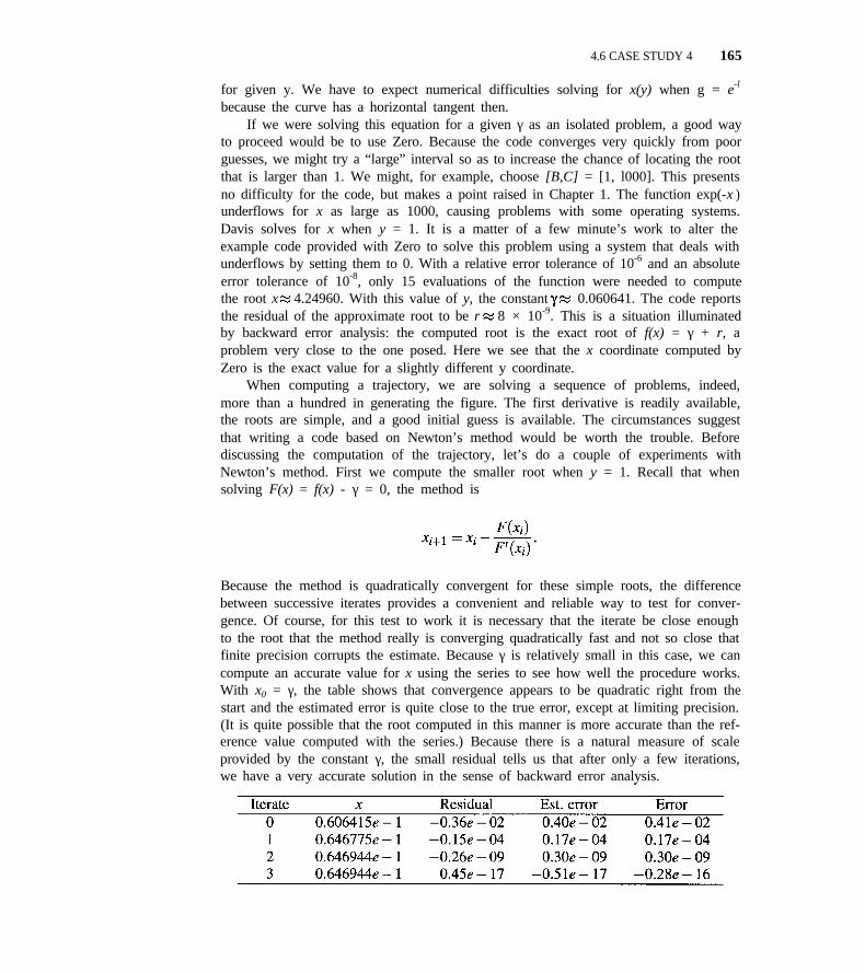
4.6 CASE STUDY 4 165
for given y. We have to expect numerical difficulties solving for x(y) when g = e-l
because the curve has a horizontal tangent then.If we were solving this equation for a given γ as an isolated problem, a good way
to proceed would be to use Zero. Because the code converges very quickly from poorguesses, we might try a “large” interval so as to increase the chance of locating the rootthat is larger than 1. We might, for example, choose [B,C] = [1, l000]. This presentsno difficulty for the code, but makes a point raised in Chapter 1. The function exp(-x )underflows for x as large as 1000, causing problems with some operating systems.Davis solves for x when y = 1. It is a matter of a few minute’s work to alter theexample code provided with Zero to solve this problem using a system that deals withunderflows by setting them to 0. With a relative error tolerance of 10-6 and an absoluteerror tolerance of 10-8, only 15 evaluations of the function were needed to computethe root x 4.24960. With this value of y, the constant 0.060641. The code reportsthe residual of the approximate root to be r 8 × 10⁻⁹. This is a situation illuminatedby backward error analysis: the computed root is the exact root of f(x) = γ + r, aproblem very close to the one posed. Here we see that the x coordinate computed byZero is the exact value for a slightly different y coordinate.
When computing a trajectory, we are solving a sequence of problems, indeed,more than a hundred in generating the figure. The first derivative is readily available,the roots are simple, and a good initial guess is available. The circumstances suggestthat writing a code based on Newton’s method would be worth the trouble. Beforediscussing the computation of the trajectory, let’s do a couple of experiments withNewton’s method. First we compute the smaller root when y = 1. Recall that whensolving F(x) = f(x) - γ = 0, the method is
Because the method is quadratically convergent for these simple roots, the differencebetween successive iterates provides a convenient and reliable way to test for conver-gence. Of course, for this test to work it is necessary that the iterate be close enoughto the root that the method really is converging quadratically fast and not so close thatfinite precision corrupts the estimate. Because γ is relatively small in this case, we cancompute an accurate value for x using the series to see how well the procedure works.With x0 = γ, the table shows that convergence appears to be quadratic right from thestart and the estimated error is quite close to the true error, except at limiting precision.(It is quite possible that the root computed in this manner is more accurate than the ref-erence value computed with the series.) Because there is a natural measure of scaleprovided by the constant γ, the small residual tells us that after only a few iterations,we have a very accurate solution in the sense of backward error analysis.
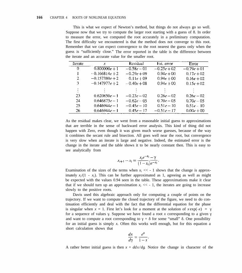
166 CHAPTER 4 ROOTS OF NONLINEAR EQUATIONS
This is what we expect of Newton’s method, but things do not always go so well.Suppose now that we try to compute the larger root starting with a guess of 8. In orderto measure the error, we computed the root accurately in a preliminary computation.The first difficulty we encountered is that the method does not converge to this root.Remember that we can expect convergence to the root nearest the guess only when theguess is “sufficiently close.” The error reported in the table is the difference betweenthe iterate and an accurate value for the smaller root.
As the residual makes clear, we went from a reasonable initial guess to approximationsthat are terrible in the sense of backward error analysis. This kind of thing did nothappen with Zero, even though it was given much worse guesses, because of the wayit combines the secant rule and bisection. All goes well near the root, but convergenceis very slow when an iterate is large and negative. Indeed, the estimated error is thechange in the iterate and the table shows it to be nearly constant then. This is easy tosee analytically from
Examination of the sizes of the terms when xi << - 1 shows that the change is approx-imately xi/(1 - xi). This can be further approximated as 1, agreeing as well as mightbe expected with the values 0.94 seen in the table. These approximations make it clearthat if we should turn up an approximation xi << - 1, the iterates are going to increaseslowly to the positive roots.
Davis used this algebraic approach only for computing a couple of points on thetrajectory. If we want to compute the closed trajectory of the figure, we need to do con-tinuation efficiently and deal with the fact that the differential equation for the phaseis singular when x = 1. First let’s look for a moment at the solution of x exp( -x) = γfor a sequence of values γ. Suppose we have found a root x corresponding to a given γand want to compute a root corresponding to γ + δ for some “small” δ. One possibilityfor an initial guess is simply x. Often this works well enough, but for this equation ashort calculation shows that
A rather better initial guess is then x + δdx/dγ. Notice the change in character of the
REFERENCES 167
problem that shows up here when x = 1. This is the kind of difficulty that we overcomewhen tracing a trajectory by exploiting additional information at our disposal.
The program that computed the figure accepts the constants a, c and the initialpoint (x,y). Using these data, it computes the constant K. The conservation law allowsus to solve for x when y is given, or to solve for y when x is given, and the code selectsthe more appropriate at each step. The differential equations for the populations tellus that for a small increment δ in t, the change in x is about δdx/dt and the change iny is about δdy/dt. If |dy/dt| < |dx/dt|, the code uses the value x + δdx/dt and solvesfor y(x). Otherwise, it uses the value y + δdy/dt and solves for x(y). This amounts tochanging the coordinate system in which the curve is viewed so as to avoid difficultieswith vertical tangents. After choosing which equation to solve, Newton’s method iseasily applied and converges very rapidly. Superlinear convergence is used to test forconvergence to a specified relative error tolerance.
REFERENCES
1. R. Borrelli and C. Coleman, Differential Equations: A Modeling Approach, Prentice Hall, En-glewood Cliffs, N.J., 1987.
2. W. Boyce and R. DiPrima, Elementary Differential Equations and Boundary Value Problems,Wiley, New York, 1992.
3. R. Brent, Algorithms for Minimization without Derivatives, Prentice Hall, Englewood Cliffs,N.J., 1973.
4. P. David and J. Voge, Propagation of Waves, Pergamon Press, New York, 1969.
5. H. Davis, Introduction to Nonlinear Differential and Integral Equations, Dover, New York,1962.
6. T. Dekker, “Finding a zero by means of successive linear interpolation,” in Constructive Aspectsof the Fundamental Theorem of Algebra, B. Dejon and P. Henrici, eds., Wiley, London, 1969.
7. J. Dennis, Jr., and R. Schnabel, Numerical Methods for Unconstrained Optimization and Non-linear Equations, Prentice Hall, Englewood Cliffs, N.J., 1983.
8. J. Eberhardt and T. Sweet, ‘The numerical solution of equations in chemistry,” J. Chem. Ed., 37(1960), pp. 422-430.
9. S. Timoshenko, Theory of Elastic Stability, McGraw Hill, New York, 1961.
10. L. Vant-Hull and A. Hildebrandt, “Solar thermal power systems based on optical transmission,”Solar Energy, 18 (1976), pp. 3l-40.
11. J. Wilkinson, Rounding Errors in Algebraic Processes, Dover, Mineola, N.Y., 1994.
12. G.M. Wing, An Introduction to Transport Theory, Wiley, New York, 1962.
MISCELLANEOUS EXERCISES FOR CHAPTER 4
4.27 A semi-infinite medium is at a uniform initial tem-perature T0 = 70°F. For time t > 0, a constant heatflux density q = 300 Btu/hr sq ft is maintained on thesurface x = 0. Knowing the thermal conductivity k =1.0 Btu/hr/ft/°F and the thermal diffusivity α = 0.04
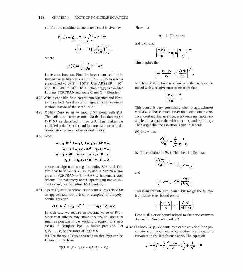
168 CHAPTER 4 ROOTS OF NONLINEAR EQUATIONS
sq ft/hr, the resulting temperature T(x, t) is given by
where
is the error function. Find the times t required for thetemperature at distances x = 0.1, 0.2, . . . ,0.5 to reach apreassigned value T = 100°F. Use ABSERR = 10-8
and RELERR = 10-6. The function erf(y) is availablein many FORTRAN and some C and C++ libraries.
4.28 Write a code like Zero based upon bisection and New-ton’s method. Are there advantages to using Newton’smethod instead of the secant rule?
4.29 Modify Zero so as to input f´(x) along with f(x).The code is to compute roots via the function u(x) =f(x)/f´(x) as described in the text. This makes themodified code faster for multiple roots and permits thecomputation of roots of even multiplicity.
4.30 Given
devise an algorithm using the codes Zero and Fac-tor/Solve to solve for x1, x2, x3 and θ. Sketch a pro-gram in FORTRAN or C or C++ to implement yourscheme. Do not worry about input/output nor an ini-tial bracket, but do define F(x) carefully.
4.31 In parts (a) and (b) below, error bounds are derived foran approximate root σ (real or complex) of the poly-nomial equation
In each case we require an accurate value of P(σ).Since root solvers may make this residual about assmall as possible in the working precision, it is nec-
Show that
a0 = (-1)nr1r2···rn
and then that
This implies that
which says that there is some zero that is approxi-mated with a relative error of no more than
This bound is very pessimistic when σ approximateswell a zero that is much larger than some other zero.To understand this assertion, work out a numerical ex-ample for a quadratic with σ r1 and |r1| >> |r2|.Then argue that the assertion is true in general.
(b) Show that
by differentiating ln P(x). This then implies that
and
This is an absolute error bound, but we get the follow-ing relative error bound easily:
How is this error bound related to the error estimatederived for Newton’s method?
essary to compute P(σ) in higher precision. Let 4.32 The book [4, p. 65] contains a cubic equation for a pa-r1,r2. . . , rn be the roots of P(x) = 0. rameter s in the context of corrections for the earth’s(a) The theory of equations tells us that P(x) can be curvature in the interference zone. The equationfactored in the form
P(x) = (x - r1)(x - r2)···(x - rn).

MISCELLANEOUS EXERCISES 169
depends on two parameters, u and v, which are ob-tamed from the heights of the towers, the distance be-tween stations, and the radius of the earth. Represen-tative values are v = 1/291, u = 30. The smallest pos-itive root is the one of interest, but calculate them all.
The residuals of the larger roots are quite large. Arethey inaccurate? Compare with Exercise 4.1. Use thecomputable error bounds of Exercise 4.31 to boundthe errors of the roots.
CHAPTER 5
NUMERICAL INTEGRATION
Approximating numerically is called numerical integration or quadrature.Most of this chapter is concerned with finite intervals [a,b], but there is some discus-sion of integrals with a and/or b infinite. Sometimes it is useful to introduce a weightfunction w(x) > 0 and so approximate integrals of the form There area number of reasons for studying numerical integration. The antiderivative of f maynot be known or may not be elementary. The integral may not be available becausethe function f is defined by values in a table or by a subprogram. Or, definite integralsmust be approximated as part of a more complicated numerical scheme, such as onefor the solution of differential equations by finite elements by means of variational orGalerkin methods.
A basic principle in numerical analysis is that if we cannot do what we want witha given function f(x), we approximate it with a function for which we can. Often theapproximating function is an interpolating polynomial. Using this principle we shallderive some basic quadrature rules and study their errors. When approximating func-tions we found that piecewise polynomial interpolants had advantages over polynomialinterpolants, and the same is true in this context. In a way piecewise polynomial in-terpolants are more natural for quadrature because using such a function amounts tobreaking up the interval of integration into pieces and approximating by a polynomialon each piece. A key idea in quadrature is to take account of the behavior of f(x)when splitting up the interval. This “adaptive” quadrature is described in Section 5.2and a code is discussed in the following section. Adaptive quadrature is the main topicof the chapter, but some attention is given to the integration of tabular data and to theintegration of functions of two independent variables. Particular attention is paid topreparing problems for their effective solution by codes of the kind developed here.
5.1 BASIC QUADRATURE RULES
To approximate
170
(5.1)
5.1 BASIC QUADRATURE RULES 171
suppose that values of f are available at N distinct points {xl,. . . ,xN}. Let PN(x) bethe polynomial that interpolates f at these points. The Lagrangian form of PN(x) leadseasily to the approximation
(5.2)
It is assumed here that the weights Ai exist. This is equivalent to the existence of theintegrals
In the case of most interest in this chapter, namely w(x) = 1, a and b finite, there is nodoubt about this. However, if the interval is infinite the approachfails because none of the xj has an integral over this interval.
The fundamental difficulty with the approach in the case of is that itis based on approximating f(x) by a polynomial, and polynomials do not have finiteintegrals over infinite intervals. For the integral of f(x) to exist, it must tend to zerorapidly as A useful device is to isolate the behavior that is different froma polynomial in a weight function that is handled analytically in the formula. Forexample, if we introduce the weight function w(x) = e-x and define F(x) = f(x)ex,the integral can be rewritten as It is straightforward to obtain formulas
for integrals of the form because the integrals exist for all j.Whether this device results in a good approximation to is a question aboutwhether F(x) behaves more like a polynomial than f(x).
Infinite intervals are one kind of problem that presents difficulties. An integrandthat is singular also presents difficulties because it does not behave like a polynomial.Often a weight function is a good way to deal with such problems. For example, in thesolution of plane potential problems by boundary element methods, it is necessary toapproximate a great many integrals of the form
(and subsequently to solve a system of linear equations to produce a numerical solutionto an integral equation of potential theory). The function ln x can be used as a weightfunction because it is nonpositive over the interval and the integrals
exist for all j (so the weight function w(x) in (5.1) can be taken to be - ln x). Similarlyto what was done with the example of an integral over an infinite interval, if we wish tocompute and f(x) behaves like ln (x) as we could introduce ln (x) as
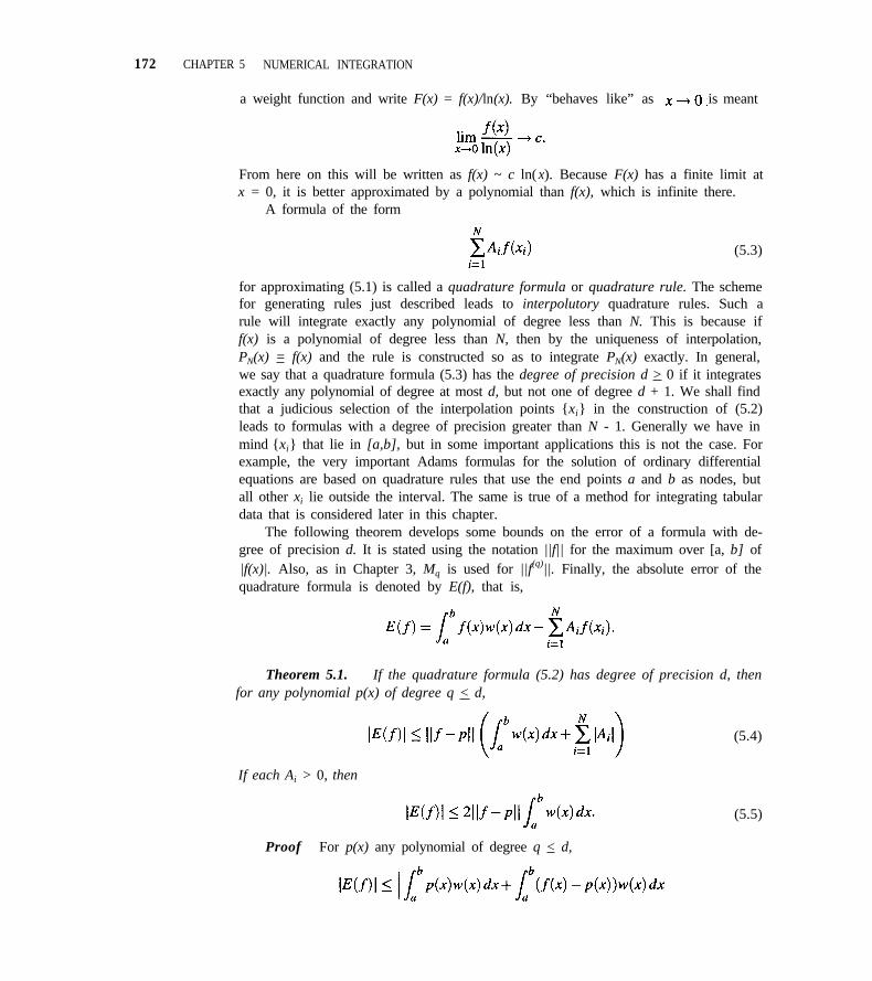
172 CHAPTER 5 NUMERICAL INTEGRATION
a weight function and write F(x) = f(x)/ln(x). By “behaves like” as is meant
From here on this will be written as f(x) ~ c ln(x). Because F(x) has a finite limit atx = 0, it is better approximated by a polynomial than f(x), which is infinite there.
A formula of the form
(5.3)
for approximating (5.1) is called a quadrature formula or quadrature rule. The schemefor generating rules just described leads to interpolutory quadrature rules. Such arule will integrate exactly any polynomial of degree less than N. This is because iff(x) is a polynomial of degree less than N, then by the uniqueness of interpolation,PN(x) = f(x) and the rule is constructed so as to integrate PN(x) exactly. In general,we say that a quadrature formula (5.3) has the degree of precision d > 0 if it integratesexactly any polynomial of degree at most d, but not one of degree d + 1. We shall findthat a judicious selection of the interpolation points {xi} in the construction of (5.2)leads to formulas with a degree of precision greater than N - 1. Generally we have inmind {xi} that lie in [a,b], but in some important applications this is not the case. Forexample, the very important Adams formulas for the solution of ordinary differentialequations are based on quadrature rules that use the end points a and b as nodes, butall other xi lie outside the interval. The same is true of a method for integrating tabulardata that is considered later in this chapter.
The following theorem develops some bounds on the error of a formula with de-gree of precision d. It is stated using the notation ||f|| for the maximum over [a, b] of|f(x)|. Also, as in Chapter 3, Mq is used for ||f(q)||. Finally, the absolute error of thequadrature formula is denoted by E(f), that is,
Theorem 5.1. If the quadrature formula (5.2) has degree of precision d, thenfor any polynomial p(x) of degree q < d,
If each Ai > 0, then
Proof For p(x) any polynomial of degree q < d,
(5.4)
(5.5)
5.1 BASIC QUADRATURE RULES 173
where we have used the fact that E(p) = 0. (Why?) This is (5.4). For (5.5), when eachAi > 0 the absolute values in (5.4) can be dropped. Because the quadrature formulaintegrates constants exactly, applying it to f(x) = 1 shows that
which results in (5.5).
Corollary 5.1. If f(x) has d + 1 continuous derivatives on [a, b], then
If each Ai > 0, then
(5.6)
(5.7)
Proof Since the bounds of Theorem 5.1 hold for any p(x), we can use the p(x)coming from Taylor’s theorem (see the appendix) with x0 = (a + b)/2 and n = q:
where
and
for some z between x0 and x. This implies that
(5.8)
Substituting this with q = d into (5.4) or (5.5) yields (5.6) or (5.7). n
When we studied polynomial interpolation, we learned that interpolants of highdegree are likely to oscillate and provide unsatisfactory fits. The situation now is dif-ferent because it is the area under the curve that is being approximated, and it seems at
174 CHAPTER 5 NUMERICAL INTEGRATION
least possible that the oscillations will average out. This is the importance of the spe-cial case of formulas with all Ai > 0. At least as far as the bound of the Theorem 5.1goes, increasing the degree of precision with such formulas can only help. Unfor-
tunately, the interpolatory quadrature formulas for based on {xi} equallyspaced in [a, b], which are called Newton-Cotes formulas, have some Ai that are neg-ative for even modest degrees. The results of these formulas may not converge to thevalue of the integral as the degree is increased. However, we shall take up another fam-ily of formulas of arbitrarily high degree of precision for which all the Ai are positive.
In the bounds (5.4), (5.5) we can choose any polynomial p(x) of any degree q < d.For finite a, b there is a polynomial p*(x) of degree at most d that is as close as possibleto f in the sense that
The code that accompanies this chapter, called Adapt, is based on two formulas withAi > 0 for all i. One has d = 5 and the other, d = 11. In the bound (5.5), in the one casewe have ||f - p*|| for the best possible approximation by a polynomial p*
5 of degree 5and in the other, p*
11 of degree 11. According to the bound, the formula of degree 11cannot be worse because the polynomial of degree 5 can be considered a polynomialof degree 11 with some zero coefficients. It would be remarkable if it were not the casethat ||f - p*
11|| is quite a bit smaller than ||f - p*5||, hence that the formula of degree 11
is quite a bit more accurate than the formula of degree 5.A more detailed analysis of the error shows that for many formulas with w(x) = 1,
including all those considered in this book, the error E(f) can be expressed as
(5.9)
for some ξ in (a,b). Note that this is an equality rather than a bound.The result (5.9) is a traditional one, but when it involves a derivative of high order,
it causes people to doubt whether the formula is practical. For instance, the formulaof degree 11 mentioned earlier satisfies (5.9) with f(12). It is hard to come to anyunderstanding of such a high order derivative, and a natural question is, What happensif you use the formula and the derivative does not exist? We appreciate now thatthe form (5.9) is just a consequence of the method of analysis. The inequality (5.8)provides bounds when f has only q + 1 continuous derivatives, and the bound basedon best approximation does not directly assume any continuous derivatives. There isno reason to fear a formula of high degree of precision because of an expression like(5.9); other expressions for its error are applicable when the function is less smooth.
If a quadrature formula has the degree of precision d, then
(5.10)
and
(5.11)
5.1 BASIC QUADRATURE RULES 175
If we assume that the error has the form (5.9), it is easy to find c from
The equations (5.10), (5.11) furnish another way to generate quadrature rules. Theapproach is known as the method of undetermined coeficients. In this approach thecoefficients {Ai} are regarded as unknowns that are found by satisfying the system oflinear equations (5.10) for d as large as possible. Before giving examples, we note thatIt is often convenient to apply the method of undetermined coefficients to a standardinterval [-1,l] and then transform to a general interval [a,b] by a simple change ofvariable. If we have
let
Then dt = (b - a)dx/2 and
Since
it follows that
so that the change of variable yields
Example 5.1. We seek a quadrature formula of the form
In the method of undetermined coefficients
f ( x ) = 1 i m p l i e s 2 = A 1 + A 2
f ( x ) = x i m p l i e s 0 = - A 1 + A 2 .
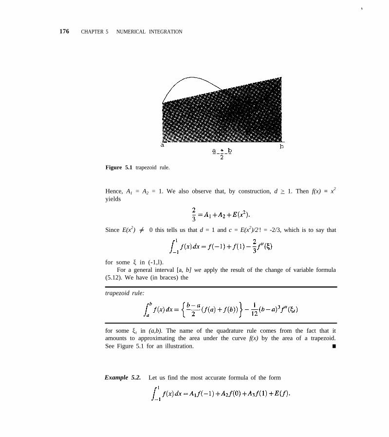
176 CHAPTER 5 NUMERICAL INTEGRATION
Figure 5.1 trapezoid rule.
Hence, A1 = A2 = 1. We also observe that, by construction, d > 1. Then f(x) = x2
yields
Since E(x2) 0 this tells us that d = 1 and c = E(x2)/2 ! = -2/3, which is to say that
for some ξ in (-1,l).For a general interval [a, b] we apply the result of the change of variable formula
(5.12). We have (in braces) the
trapezoid rule:
for some ξt in (a,b). The name of the quadrature rule comes from the fact that itamounts to approximating the area under the curve f(x) by the area of a trapezoid.See Figure 5.1 for an illustration. n
Example 5.2. Let us find the most accurate formula of the form
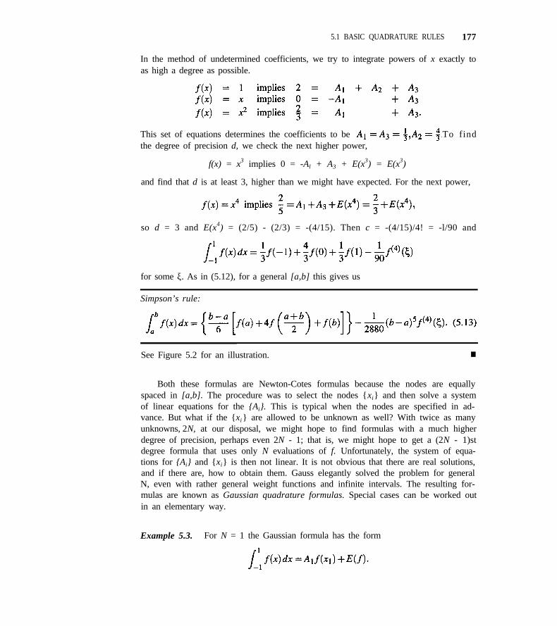
5.1 BASIC QUADRATURE RULES 177
In the method of undetermined coefficients, we try to integrate powers of x exactly toas high a degree as possible.
This set of equations determines the coefficients to be To findthe degree of precision d, we check the next higher power,
f(x) = x3 implies 0 = -Al + A3 + E(x3) = E(x3)
and find that d is at least 3, higher than we might have expected. For the next power,
so d = 3 and E(x4) = (2/5) - (2/3) = -(4/15). Then c = -(4/15)/4! = -l/90 and
for some ξ. As in (5.12), for a general [a,b] this gives us
Simpson’s rule:
See Figure 5.2 for an illustration. n
Both these formulas are Newton-Cotes formulas because the nodes are equallyspaced in [a,b]. The procedure was to select the nodes {xi} and then solve a systemof linear equations for the {Ai}. This is typical when the nodes are specified in ad-vance. But what if the {xi} are allowed to be unknown as well? With twice as manyunknowns, 2N, at our disposal, we might hope to find formulas with a much higherdegree of precision, perhaps even 2N - 1; that is, we might hope to get a (2N - 1)stdegree formula that uses only N evaluations of f. Unfortunately, the system of equa-tions for {Ai} and {xi} is then not linear. It is not obvious that there are real solutions,and if there are, how to obtain them. Gauss elegantly solved the problem for generalN, even with rather general weight functions and infinite intervals. The resulting for-mulas are known as Gaussian quadrature formulas. Special cases can be worked outin an elementary way.
Example 5.3. For N = 1 the Gaussian formula has the form
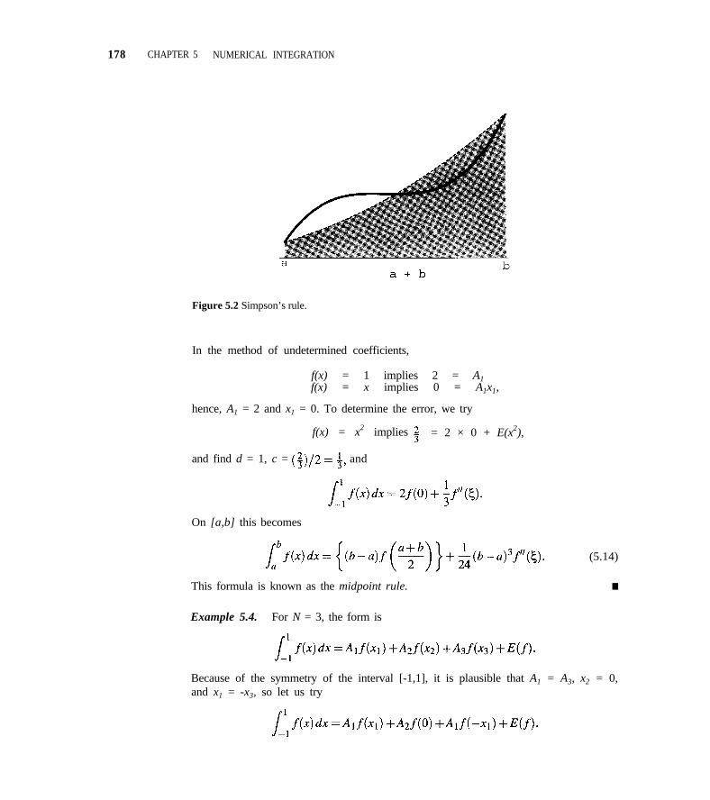
178 CHAPTER 5 NUMERICAL INTEGRATION
Figure 5.2 Simpson’s rule.
In the method of undetermined coefficients,
f(x) = 1 implies 2 = A1f(x) = x implies 0 = A1x1,
hence, A1 = 2 and x1 = 0. To determine the error, we try
f(x) = x2 implies = 2 × 0 + E(x2),
and find d = 1, c = and
On [a,b] this becomes
This formula is known as the midpoint rule.
(5.14)
n
Example 5.4. For N = 3, the form is
Because of the symmetry of the interval [-1,1], it is plausible that A1 = A3, x2 = 0,and x1 = -x3, so let us try
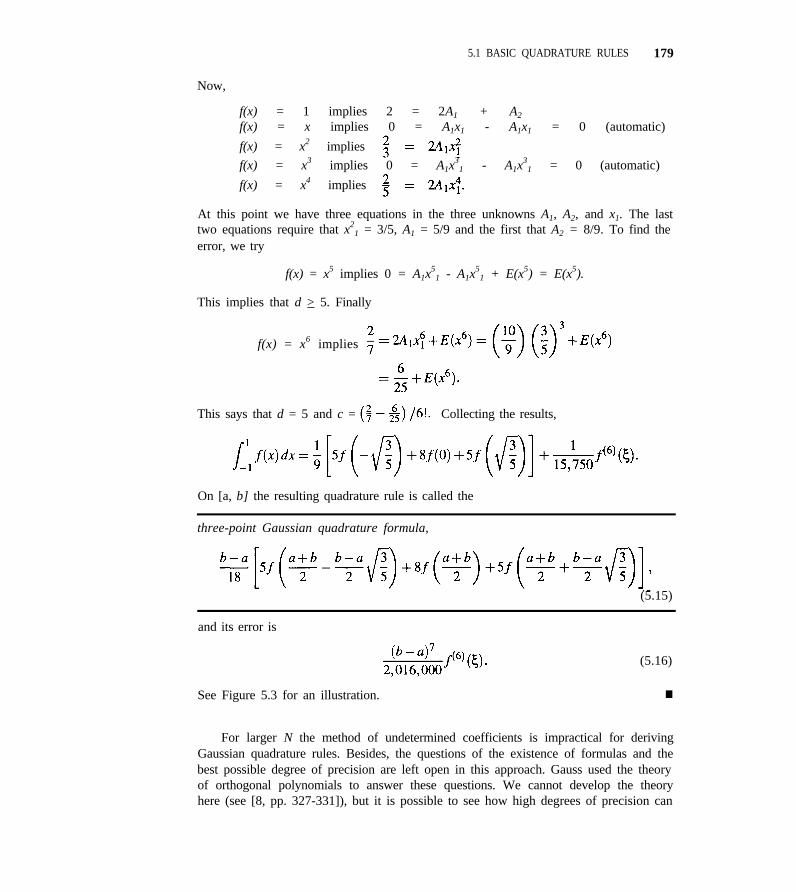
5.1 BASIC QUADRATURE RULES 179
Now,
f(x) = 1 implies 2 = 2A1 + A2
f(x) = x implies 0 = A1x1 - A1x1 = 0 (automatic)
f(x) = x2 implies
f(x) = x3 implies 0 = A1x3
1 - A1x3
1 = 0 (automatic)
f(x) = x4 implies
At this point we have three equations in the three unknowns A1, A2, and x1. The lasttwo equations require that x2
1 = 3/5, A1 = 5/9 and the first that A2 = 8/9. To find theerror, we try
f(x) = x5 implies 0 = A1x5
1 - A1x5
1 + E(x5) = E(x5).
This implies that d > 5. Finally
f(x) = x6 implies
This says that d = 5 and c = Collecting the results,
On [a, b] the resulting quadrature rule is called the
three-point Gaussian quadrature formula,
(5.15)
and its error is
(5.16)
See Figure 5.3 for an illustration. n
For larger N the method of undetermined coefficients is impractical for derivingGaussian quadrature rules. Besides, the questions of the existence of formulas and thebest possible degree of precision are left open in this approach. Gauss used the theoryof orthogonal polynomials to answer these questions. We cannot develop the theoryhere (see [8, pp. 327-331]), but it is possible to see how high degrees of precision can
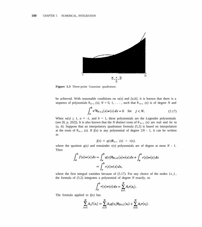
180 CHAPTER 5 NUMERICAL, INTEGRATION
Figure 5.3 Three-point Gaussian quadrature.
be achieved. With reasonable conditions on w(x) and [a,b], it is known that there is asequence of polynomials θN+1 (x), N = 0, 1, . . . , such that θ N+1 (x) is of degree N and
(5.17)
When w(x) = 1, a = -1, and b = 1, these polynomials are the Legendre polynomials(see [8, p. 202]). It is also known that the N distinct roots of θ N+1 (x) are real and lie in(a, b). Suppose that an interpolatory quadrature formula (5.2) is based on interpolationat the roots of θN+1 (x). If f(x) is any polynomial of degree 2N - 1, it can be writtenas
f(x) = q(x)θθN+l (x) + r(x),
where the quotient q(x) and remainder r(x) polynomials are of degree at most N - 1.Then
where the first integral vanishes because of (5.17). For any choice of the nodes {x i} ,the formula of (5.2) integrates a polynomial of degree N exactly, so
The formula applied to f(x) has
5.1 BASIC QUADRATURE RULES 181
Now we use the fact that the xi are roots of θ n(x) to see that
Since any polynomial f(x) of degree 2N - 1 is integrated exactly, this formula has adegree of precision that is at least 2N - 1.
There are computationally convenient ways to derive Gaussian quadrature rules,and formulas may be found in specialized books. Gaussian formulas are valuable be-cause they provide the highest degree of precision for the number of values of f(x).An important fact about Gaussian formulas is that the Ai are all positive. As discussedin connection with the error bounds, this means that we can use formulas of a very highdegree of precision, even for integrands that are not smooth. Gaussian formulas incor-porating weight functions are especially valuable tools for dealing with integrands thatare singular and intervals that are infinite. Whether or not there is a weight function,the nodes of a Gaussian formula all lie in the interior of [a, b]. This means that theformula does not use f(a) or f(b). We shall see that this is quite helpful in dealingwith singular integrands.
So far we have been considering procedures based on approximating f(x) over thewhole interval [a,b]. Just as with polynomial interpolation, the error depends stronglyon the length of the interval. This suggests that we break up the interval and so approx-imate the function by a piecewise polynomial function rather than a single polynomial.The simplest approach is to split the interval into pieces specified in advance. If wepartition [a,b] into a = x1 < x2 < ··· < xn+1 = b, thenand we can apply standard quadrature rules to each of the n integrals. The resultingformula is known as a composite or compound rule. Traditionally the {xi} have beenchosen to be equally spaced in [a,b] and the same formula used on each piece, but thisis not necessary.
Example 5.5. Composite Trapezoid Rule. The composite trapezoid rule approxi-mates I = by splitting [a,b] into n pieces of length h = (b - a)/n and apply-ing the trapezoid rule to each piece. With the definition xi = a + ih, this is
which simplifies to
Figure 5.4 illustrates the composite trapezoid rule. n
An ingenious use of repeated integration by parts establishes the Euler-Maclaurinsum formula. It states that if f(2v)(x) is continuous on [a,b], then

182 CHAPTER 5 NUMERICAL INTEGRATION
Figure 5.4 Composite trapezoid rule.
for some x in [a,b]. The coefficients B2k appearing here are known as the Bernoullinumbers. The first few terms of the error expansion are
The basic trapezoid rule applied to an interval of length h has an error that goes to zerolike h3. When the n = 1/h terms are combined, the error of the approximation to theintegral goes to zero like h2. However, notice that if it should happen that f(1)(b) =f(1)(a), the formula is more accurate than usual. If in addition other derivatives havethe same values at the ends of the interval, the formula is still more accurate. Whenintegrating a periodic function over a multiple of a period, all the derivatives at theends of the interval are equal and this formula is extraordinarily accurate. In fact, ifthe periodic function is analytic, so that it has derivatives of all orders, Tn I fasterthan any power of h! Although rather special, this is extremely important in the contextof Fourier analysis.
The error of Tn can be estimated by comparing it to the more accurate result T2n
obtained by halving each subinterval. A convenient way to evaluate the formula is
where
It is important to note that all the evaluations of f made in forming Tn are reused inT2n.
There is a way of exploiting the error expansion of the composite trapezoid ruledue to Romberg that is popular for general integrands. The idea is to combine Tn and
5.1 BASIC QUADRATURE RULES 183
T2n in such a way as to obtain a higher order result. According to the error expansion,
A little manipulation then shows that
The formula
is of higher order than each of the individual formulas. As it turns out, this formulais the composite Simpson’s rule. Romberg developed a computationally convenientway of successively combining results so as to increase the order by two with eachcomputation of a composite trapezoid rule. The process is called extrapolation.
Romberg integration can be very effective. It adapts the order of the method tothe problem. It does, however, depend on the integrand being smooth throughout theinterval. Also, it evaluates at the ends of the interval, which is sometimes inconvenient.MATHCAD uses Romberg integration for quadrature. If there is a singularity at an endof an interval or if the process does not converge, the code switches to a variant basedon the midpoint rule that does not evaluate at the ends of the intervals and dividesintervals by 3 rather than 2. n
E X E R C I S E S
5.1 Use the method of undetermined coefficients to deriveNewton’s
Calculate A1, A2, A3, A4, d, and c in the usual manner.
5.2 Use the method of undetermined coefficients to findthe two-point Gaussian quadrature formula with its as-sociated error. Begin with
and calculate A1 and x1 in the usual manner. Assum-ing E(f) = cf(d+1)(ξ), find d and c. What is the cor-responding formula and associated error on the gen-eral interval [a,b]?
5.3 Implement the composite trapezoid rule and apply itto
Of course, you must choose h small enough that sam-ples are taken in each period. Approximate the inte-gral for a number of values of h that tend to 0. Accord-ing to the theory of Example 5.5, the approximationsTn ought to converge extremely fast. Is that what youfind?
184 CHAPTER 5 NUMERICAL INTEGRATION
5.2 ADAPTIVE QUADRATURE
In this section a code is developed that approximates I = to an accuracyspecified by the user. This is done by splitting the interval [a,b] into pieces and apply-ing a basic formula to each piece. The interval is split in a way adapted to the behaviorof f(x). A fundamental tool is an error estimate. With the capability of estimating theerror of integrating over a subinterval, we ask if the error is acceptable, and if it is not,the subinterval is split again. As we have seen, for a formula of even modest degree ofprecision, reducing the length of the interval increases substantially the accuracy of theapproximation. Proceeding in this manner, the formula is applied over long subinter-vals where f(x) is easy to approximate and over short ones where it is difficult. Codeslike the one developed here are in very wide use, being found, for example, in thecollection of state-of-the-art codes QUADPACK [12], libraries like NAG and IMSL,and computing environments like MATLAB.
When the code is supplied absolute and relative error tolerances ABSERR andRELERR, it attempts to calculate a value ANSWER such that
|I - ANSWER| < max(ABSERR, RELERR × |I|).
The computational form of this uses an error estimate
and replaces I by ANSWER:
|ERREST| < max(ABSERR, RELERR × |ANSWER|). (5.18)
We cannot hope to get a more accurate approximate integral than the correctly roundedtrue value, so it makes no sense to take RELERR < u, the unit roundoff of the computerused. Indeed, we require RELERR > 10u so that we do not work with error estimatesthat are nothing but roundoff. We also require ABSERR > 0 so as to deal with the raresituation that I = 0.
The method employed in the code breaks the interval [a,b] into pieces [α,β] onwhich the basic quadrature rule is sufficiently accurate. To decide this we must beable to estimate the error of the rule. This is done with a basic principle of numericalanalysis, namely to estimate the error of a result by comparing it to a more accurateresult. Besides the approximation
another approximation is formed that is believed to be more accurate. Then
says that when is more accurate than the error in is approximately equal to
5.2 ADAPTIVE QUADRATURE 185
To keep down the cost of estimating the error, we use evaluations of f(x) in bothformulas. As a simple example, we might take Q to be the trapezoid rule and to beSimpson’s rule. The trapezoid rule is based on the values f (α) and f(β). The errorestimate is computed with Simpson’s rule, which needs only the one additional value
f((α+β) /2 Simpson’s rule is considerably more accurate than the trapezoid rule,giving us reason to hope that the estimate will be a good one.
The code Adapt uses for Q the three-point Gaussian quadrature formula of Ex-ample 5.4 that has degree of precision d1 = 5. A formula of much higher degree ofprecision is used for The error analysis based on best possible polynomial approx-imation gives us confidence that will be more accurate than Q. It would be possibleto use another Gaussian rule for but the N-point Gaussian rule for N 3 uses Ncompletely different {xi} (except possibly x = 0). To keep the number off evaluationsto a minimum, another approach is taken. In 1964 Kronrod derived for each N-pointGaussian rule a corresponding rule of degree 3N + 1 or 3N + 2 (depending on whetherN is even or odd). The idea was to start with the N Gaussian nodes and add N + 1others chosen to obtain the highest possible degree of precision. Formulas for N < 40are tabulated in [10]. The N = 3 case is
where
x1 = (as for three-point Gaussian quadrature)
x2 = 0.9604912687080202
x3 = 0.4342437493468026
A1 = 0.2684880898683334
A2 = 0.1046562260264672
A3 = 0.4013974147759622
A4 = 0.4509165386584744.
The basic idea of adaptive quadrature is to approximate the integral over a subin-terval (α,β). If the approximation is not accurate enough, the interval is split into(usually) two parts and the integral approximated over each subinterval. Eventually,accurate approximations are computed on all the subintervals of [a,b] that are addedup to approximate the integral over [a,b] or the cost is deemed too high and the compu-tation terminated. The error terms of the formulas quantify the benefit of splittingan interval; recall from (5.16) that
The corresponding result for the Kronrod formula of seven points is
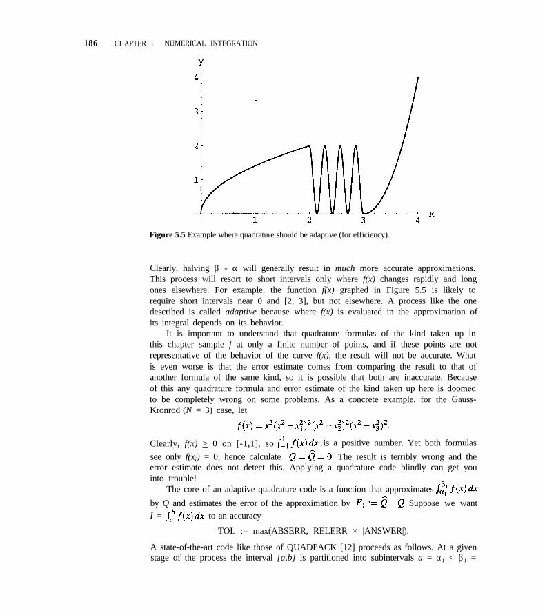
186 CHAPTER 5 NUMERICAL INTEGRATION
Figure 5.5 Example where quadrature should be adaptive (for efficiency).
Clearly, halving β - α will generally result in much more accurate approximations.This process will resort to short intervals only where f(x) changes rapidly and longones elsewhere. For example, the function f(x) graphed in Figure 5.5 is likely torequire short intervals near 0 and [2, 3], but not elsewhere. A process like the onedescribed is called adaptive because where f(x) is evaluated in the approximation ofits integral depends on its behavior.
It is important to understand that quadrature formulas of the kind taken up inthis chapter sample f at only a finite number of points, and if these points are notrepresentative of the behavior of the curve f(x), the result will not be accurate. Whatis even worse is that the error estimate comes from comparing the result to that ofanother formula of the same kind, so it is possible that both are inaccurate. Becauseof this any quadrature formula and error estimate of the kind taken up here is doomedto be completely wrong on some problems. As a concrete example, for the Gauss-Kronrod (N = 3) case, let
Clearly, f(x) > 0 on [-1,1], so is a positive number. Yet both formulas
see only f(xi) = 0, hence calculate The result is terribly wrong and theerror estimate does not detect this. Applying a quadrature code blindly can get youinto trouble!
The core of an adaptive quadrature code is a function that approximates
by Q and estimates the error of the approximation by Suppose we wantI = to an accuracy
TOL := max(ABSERR, RELERR × |ANSWER|).
A state-of-the-art code like those of QUADPACK [12] proceeds as follows. At a givenstage of the process the interval [a,b] is partitioned into subintervals a = α1 < β1 =
5.2 ADAPTIVE QUADRATURE 187
α2 < β2 = α3 < ··· < βN = b; there is an estimate Qj available for the integral off(x) over each subinterval [αj ,β j] and an estimate Ej available of the error of Qj. Byadding up the Qj and Ej, an approximation Q = ANSWER to I is available along withan estimate E = ERREST of its error. If the current approximation to I is not goodenough, the subinterval [αj, β j] with the largest error |Ej| is selected for improvement.It is split into two pieces [αj, (αj + β j) /2], [(αj + β j) /2, β j ], and approximate integralsover these pieces and estimates of their error are computed. The two subintervals andthe associated quantities replace the subinterval [αj, β j ] and its associated quantities.This global adaptive procedure is extremely efficient, but at a cost of keeping trackof all the subintervals and the information associated with them. In the code Adaptthe adaptation is more local and the implementation a little simpler. The differencein Adapt is that when a subinterval is integrated with enough accuracy, it is no longera candidate for improvement. Thus a queue is kept of subintervals on which the es-timated error of the integral over the subinterval is considered to be too large. At atypical stage of the process, the code tests whether the current approximation to I issufficiently accurate to satisfy the user’s error request. If it is not, the next subinterval[αj, β j] is removed from the queue, split in half, and approximations to the integralover each half, along with error estimates, are computed. They are placed at the end of
the queue. If an approximation to an integral is estimated to have an errorno more than |(β - α) / (b - a)] × TOL, it is accepted and [α, β] is not examined again.This is more stringent than necessary because adding up approximations
that satisfy this condition will result in an error such that
The global adaptation used in the collection QUADPACK [12] subdivides untilTOL. The more local adaptation of Adapt subdivides until TOL. Because
is always at least as big as and perhaps much larger, the local processworks harder but should provide answers that are more accurate than the specifiedtolerance TOL.
Let us now formalize the algorithm. To start the process, form the approximationQ to the integral over [a,b] and its estimated error ERREST. If |ERREST| < TOL, wetake ANSWER = Q as the result and return. If ERREST does not pass the error test,a, b, Q, and E = ERREST are placed in the queue and the following loop is entered:
remove α, β, Q, E from top of queue
compute QL with estimated error EL
compute QR with estimated error ERANSWER := ANSWER + (( QL + QR) - Q)ERREST := ERREST + ((EL + ER) - E)if EL is too big, add α, (α + β)/2, QL, EL to end of queueif ER is too big, add (α + β)/2, β, QR, ER to end of queue.
188 CHAPTER 5 NUMERICAL, INTEGRATION
This procedure is repeated until one of the following events occurs:
1. The queue becomes empty.
2. |ERREST| < TOL.
3. The queue becomes larger than the space allocated.
4. Too many f evaluations are made.
The first two cases represent a success. The last two represent a failure in the sensethat the code has failed to achieve the desired accuracy in the work allotted. It maybe that the estimated error, although larger than specified by means of the tolerances,is acceptable and the answer reported will suffice. Even when it is not, an inaccuratevalue of the integral may be useful as a indication of the size of the integral whenselecting appropriate tolerances.
Notice the way quantities have been grouped in the computation of ANSWER andERREST. The quantity Q and the sum QL + QR both approximate the integral off over[α, β]. They normally agree in a few leading digits, so their difference involves cancel-lation and is computed without arithmetic error. Because the difference is normally asmall correction to ANSWER, it is possible to make a great many corrections withoutaccumulation of arithmetic error. If the quantities are not grouped, the correction of a“small” ANSWER may be inaccurate.
5.3 CODES FOR ADAPTIVE QUADRATURE
The code presented here uses the three-point Gaussian rule to estimate integrals alongwith the seven-point Kronrod rule to estimate errors. In FORTRAN the routine Adapthas a typical call
CALL ADAPT (F, A, B, ABSERR, RELERR, ANSWER, ERREST, FLAG)
and in C++,
flag = Adapt(f, a, b, abserr, relerr, answer, errest);
and it is
flag = Adapt(f, a, b, abserr, relerr, &answer, &errest);
in the C version.
The first argument, F or f, is the name of the function that provides values ofthe integral. In FORTRAN F must be declared in an EXTERNAL statement. Thenext four variables are input parameters: A and B are the (finite) end points of theintegration interval, ABSERR and RELERR are the required absolute and relative er-ror tolerances. The remaining variables are output quantities: ANSWER contains theapproximation to the integral and ERREST an estimate for the error of the approxi-mation. The value of FLAG is 0 for a normal return with (5.18) satisfied. FLAG > 0
5.3 CODES FOR ADAPTIVE QUADRATURE 189
signals that there was not enough storage for the queue, or that too many function eval-uations were needed. Illegal input (ABSERR < 0 or RELERR < 10u) is indicated byFLAG = -1. In C and C++ the value of flag is the return value of the function Adapt.
Example 5.6. Let us try the code on a problem with an analytical integral, for ex-ample, for which I = e - 1 = 1.71828182845904. Its output for a requested
accuracy of ABSERR= 10 -5 and RELERR = 10 -8 follows.
FLAG = 0Approximate value of the integral = 1.718281004372522Error in ANSWER is approximately 8.240865232136876E-007
7 evaluations of F were required.
Routine Adapt evaluates f at least seven times, so the code found this task to be veryeasy. It is seen that ERREST approximates the true error of 0.82408652 × 10⁻⁶ ex-t r e m e l y w e l l . n
Example 5.7. A more interesting problem is to estimate againwith ABSERR = 10-5, RELERR = 10-8. Although continuous at x = 0, the integrandhas infinite derivatives there, so it does not behave like a polynomial near this point.An adaptive code deals with this by using short intervals near the point. Applicationof the Adapt code results in
FLAG = 0Approximate value of the integral = 6.718072986891337E-001Error in ANSWER is approximately -6.448552584540975E-005
119 evaluations of F were required.
The techniques of the next section can be used to produce an accurate value of I =0.671800032402 for the integral, which tells us that the actual error is about -0.73 x10⁻⁵. In comparison to Example 5.6, this problem required many more evaluations off, and ERREST is not nearly as accurate. It should be appreciated that all we need is arough approximation to the error, so this one is perfectly acceptable. It is instructive tosee how Adapt samples the integrand in this example. In Figure 5.6 ordered pairs (x,y)are plotted (as are pairs (x, 0) along the x-axis); x is a sampling point used by Adapt andy the corresponding value of the integrand. Notice how the points congregate aroundthe singularity at zero as the theory predicts they should. n
EXERCISES
Unless otherwise indicated, use as tolerances AB- (b) x1/10
SERR = 10-8 and RELERR = 10-6 for the comput-ing exercises. (c) 1/[(3x - 2)2]
5.4 To test out Adapt try the following integrands.
(a) 4/(1 + x2) (d) 1 + sin2 38πx
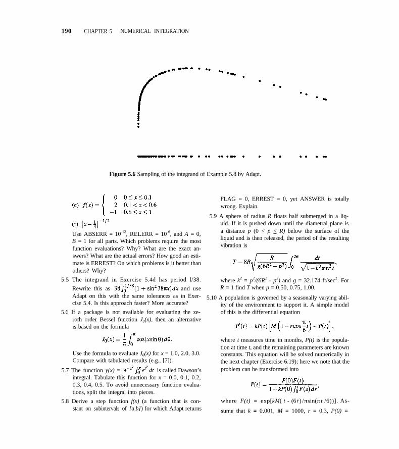
190 CHAPTER 5 NUMERICAL INTEGRATION
Figure 5.6 Sampling of the integrand of Example 5.8 by Adapt.
Use ABSERR = 10-12, RELERR = 10-6, and A = 0,B = 1 for all parts. Which problems require the mostfunction evaluations? Why? What are the exact an-swers? What are the actual errors? How good an esti-mate is ERREST? On which problems is it better thanothers? Why?
5.5 The integrand in Exercise 5.4d has period l/38.
Rewrite this as and useAdapt on this with the same tolerances as in Exer-cise 5.4. Is this approach faster? More accurate?
5.6 If a package is not available for evaluating the ze-roth order Bessel function J0(x), then an alternativeis based on the formula
Use the formula to evaluate J0(x) for x = 1.0, 2.0, 3.0.Compare with tabulated results (e.g., [7]).
5.7 The function y(x) = is called Dawson’sintegral. Tabulate this function for x = 0.0, 0.1, 0.2,0.3, 0.4, 0.5. To avoid unnecessary function evalua-tions, split the integral into pieces.
5.8 Derive a step function f(x) (a function that is con-stant on subintervals of [a,b]) for which Adapt returns
FLAG = 0, ERREST = 0, yet ANSWER is totallywrong. Explain.
5.9 A sphere of radius R floats half submerged in a liq-uid. If it is pushed down until the diametral plane isa distance p (0 < p < R) below the surface of theliquid and is then released, the period of the resultingvibration is
where k2 = p2/(6R2 - p2) and g = 32.174 ft/sec2. ForR = 1 find T when p = 0.50, 0.75, 1.00.
5.10 A population is governed by a seasonally varying abil-ity of the environment to support it. A simple modelof this is the differential equation
where t measures time in months, P(t) is the popula-tion at time t, and the remaining parameters are knownconstants. This equation will be solved numerically inthe next chapter (Exercise 6.19); here we note that theproblem can be transformed into
where F(t) = exp[kM( t - (6r) /πsin(π t /6))]. As-
sume that k = 0.001, M = 1000, r = 0.3, P(0) =
5.4 SPECIAL DEVICES FOR INTEGRATION 191
5.11
5.12
250 and use Adapt efficiently to table P(t) for t =0, 3, 6, 9,. . . , 36.
Examine the effect of noise on Adapt as follows. Forthe input function F(x) use
T 1 := f(x) × 10n
T 2 := T1 + f(x)
F(x) := T2- T1
where f(x) is the original integrand (use some of theexamples in Exercise 5.4). With ABSERR = REL-ERR (u the unit roundoff) try
and then n What is the behavior? Doesthe algorithm appear to be stable?
To solve the nonlinear two-point boundary value prob-lem
using standard initial value problem codes (e.g., Rke),it is necessary to find the missing initial condition
y´(0). Observing that y´´ = exp(y) - 1 can be writtenin the form
we can integrate to obtain
Since y(0) = 0, this says y´(0) = Solving fory´(x) (by separation of variables) yields
which, when evaluated at x = 1, becomes
Use Adapt and Zero to find c and then y´(0).
5.4 SPECIAL DEVICES FOR INTEGRATION
Quadrature formulas approximate integrals using a finite number of samples. If thesamples are not representative, the result may be inaccurate despite an estimated errorthat is acceptable. Put differently, the approximate integral and its error estimate arebased on an assumption that the integrand changes smoothly between samples. Adap-tive codes generally do very well at recognizing the behavior of integrands, but f(x)with sharp peaks or many oscillations in the interval present special difficulties. Some-times it is necessary to assist a code by breaking up the interval of integration yourselfso as to ensure that the code will take samples in critical areas. A contrived examplewill help make the point.
The family of integrals
can be evaluated readily with the recurrence
When n is large, the integrand has a sharp peak at the midpoint of the interval. Withtolerances of ABSERR = 10-5 and RELERR = 10-11, for n = 200 Adapt returnedANSWER = 0.1252567600019366 and an estimated error of about -3.654 × 10⁻⁶ ata cost of 203 evaluations of the integrand. The true error is about -3.654 × 10⁻⁶. Thecode had no difficulty producing an accurate answer and an excellent error estimatebecause it samples at the midpoint and “sees” the peak. However, if the interval is split
192 CHAPTER 5 NUMERICAL INTEGRATION
into [0,2.6] and [2.6,π], the results are quite different. Integrating over the two inter-vals and adding the results provides an approximate integral of 4.111202459491848 ×10⁻⁷ and an estimated error of about -1.896 × 10⁻⁷ at a cost of 14 evaluations of theintegrand. The code has been completely fooled! This happened because the initialsamples did not reveal the presence of the peak. The code took the minimum numberof samples from each interval, namely seven, showing that it believed the problem tobe very easy. When this happens it is prudent to consider whether you agree that theproblem is very easy and if not, to break up the interval into pieces that will cause thecode to “see” the behavior of the integrand. Of course, one must be careful how to dothis breaking into pieces, as [0,2.6] and [2.6,π] won’t do for this problem.
Adapt is based on approximation by polynomials over finite intervals. As a con-sequence it may have to resort to a great many subintervals to integrate functions thatdo not behave like a polynomial near a critical point or to integrate functions over aninfinite interval. Gaussian quadrature formulas with a suitable weight function are agood way to handle such problems. Specific formulas can be found in sources like[13]. Substantial collections of quadrature codes such as those of QUADPACK, NAG,and IMSL contain specialized routines for a variety of difficulties. In this section wediscuss some techniques for preparing problems to make them more suitable for ageneral-purpose code like Adapt. With a little mathematical effort, a problem that thecode cannot solve might be put into a form that it can solve, and problems that it cansolve are solved more efficiently.
OSCILLATORY INTEGRANDSIf the integral f(x) is periodic with period p, that is, f(x + p) = f(x) for all x, andb - a is some integer multiple of p, the integration should be performed over just oneperiod (or sometimes less) and symmetry used for the remainder. For example, for theintegral in Exercise 5.3,
If you have worked Exercise 5.3 you should have found that the composite trapezoidrule is very efficient; consequently, if you have many functions to be integrated over aperiod, it is advisable to use a special-purpose code based on the composite trapezoidalrule.
Oscillatory nonperiodic functions are more difficult. Generally the integral shouldbe split into subintervals so that there are few oscillations on each subinterval. Adaptmay do this automatically, but the computation can be made more reliable and possiblyless expensive by a little analysis. As an example, let us estimate
This integral could be rewritten many ways, one of which is
5.4 SPECIAL DEVICES FOR INTEGRATION 193
Proceeding in this manner, Adapt is called 20 times, but on each interval the inte-grand has constant sign and varies smoothly between samples. This is a reasonableway to deal with a single integral of this kind, but in contexts like Fourier analysis,where many functions having the form of a periodic function times a nonperiodicfunction need to be integrated, it is better to use special-purpose formulas such asproduct quadrature. This particular example is treated in Case Study 3 where the useof the general-purpose code Adapt is contrasted with Filon’s method for finite Fourierintegrals.
INFINITE INTEGRATION INTERVALAdapt cannot be applied directly to because it deals only with finite inter-vals. One way to apply the code is to use the definition
The idea is to determine an analytical bound for the tail With it an end
point b can be selected large enough that equals to the accuracyrequired. It does not matter if b is rather larger than necessary, so a crude bound forthe tail will suffice.
Another way to get to a finite interval is to change the variable of integration. Forexample, to estimate the new variable s = 1/x yields the equivalent
integral on a finite interval. Generally this trades one difficulty(an infinite interval) for another (a singularity at an end point). For this particularexample, so the integrand is continuous at s = 0 andAdapt can be applied directly. If the original problem were thens = x-1
would not help because it produces the same infinite interval. The choices = e-x leads to for which the integrand approaches 0 asOn the integration interval the transformation s = arctan x is often useful.
SINGULAR INTEGRANDSBy a singularity we mean a point where the function or a low order derivative is dis-continuous. There are two cases: (1) finite jumps and (2) infinite values. In either case,if there is a known singularity at a point c in (a,b), a basic tactic is to split the intervalinto (a,c) and (c,b). In this way we can arrange that we approximate integrals withintegrands that are finite except possibly at one end.
If f(x) is finite at the singularity (as for step functions), Adapt can be used on eachpiece and the results added to produce an approximation to This is clearenough, but it must be kept in mind that a function that is smooth to the eye may not besmooth to the code. Surprisingly often someone integrates a spline with a quadratureroutine. Of course, such an integration should be done analytically, but it may beconvenient to resort to an adaptive quadrature routine. Just remember that splines havediscontinuities in low order derivatives. If a routine like Adapt is applied to each pieceof a piecewise polynomial function, it will have no difficulty. Indeed, it will be exact
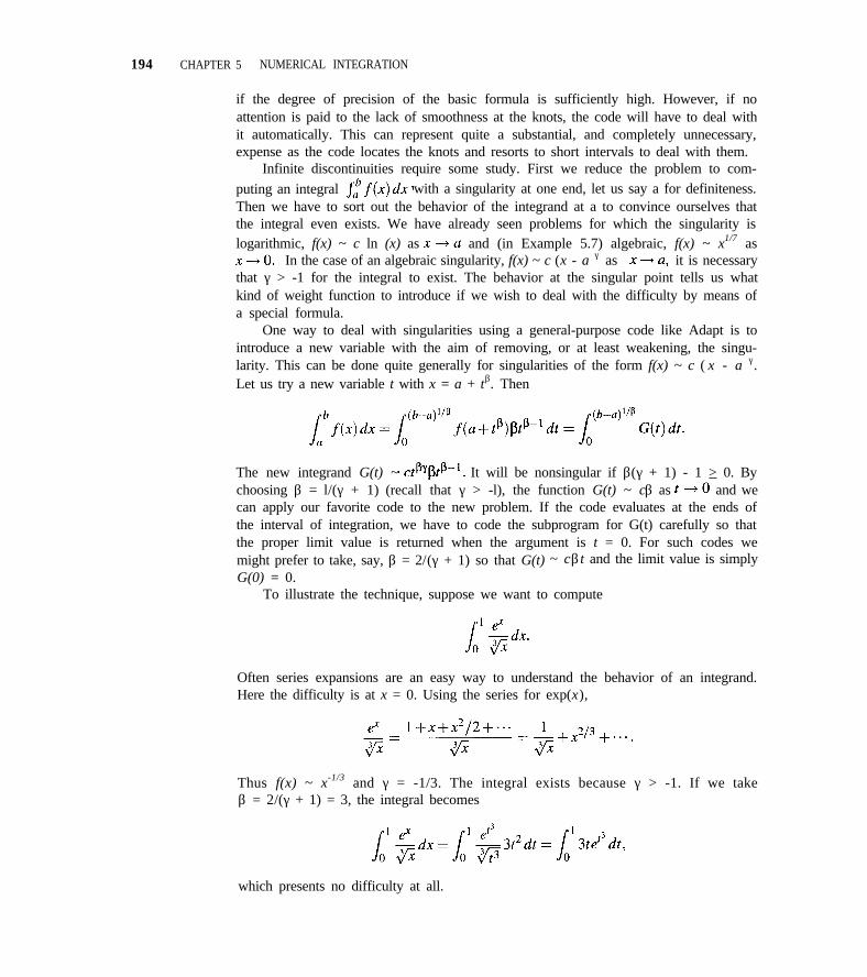
194 CHAPTER 5 NUMERICAL INTEGRATION
if the degree of precision of the basic formula is sufficiently high. However, if noattention is paid to the lack of smoothness at the knots, the code will have to deal withit automatically. This can represent quite a substantial, and completely unnecessary,expense as the code locates the knots and resorts to short intervals to deal with them.
Infinite discontinuities require some study. First we reduce the problem to com-
puting an integral with a singularity at one end, let us say a for definiteness.Then we have to sort out the behavior of the integrand at a to convince ourselves thatthe integral even exists. We have already seen problems for which the singularity islogarithmic, f(x) ~ c ln (x) as and (in Example 5.7) algebraic, f(x) ~ x1/7 as
In the case of an algebraic singularity, f(x) ~ c (x - a)γ as it is necessarythat γ > -1 for the integral to exist. The behavior at the singular point tells us whatkind of weight function to introduce if we wish to deal with the difficulty by means ofa special formula.
One way to deal with singularities using a general-purpose code like Adapt is tointroduce a new variable with the aim of removing, or at least weakening, the singu-larity. This can be done quite generally for singularities of the form f(x) ~ c ( x - a) γ.Let us try a new variable t with x = a + tβ. Then
The new integrand G(t) ~ It will be nonsingular if β(γ + 1) - 1 > 0. Bychoosing β = l/(γ + 1) (recall that γ > -l), the function G(t) ~ cβ as and wecan apply our favorite code to the new problem. If the code evaluates at the ends ofthe interval of integration, we have to code the subprogram for G(t) carefully so thatthe proper limit value is returned when the argument is t = 0. For such codes wemight prefer to take, say, β = 2/(γ + 1) so that G(t) ~ cβ t and the limit value is simplyG(0) = 0.
To illustrate the technique, suppose we want to compute
Often series expansions are an easy way to understand the behavior of an integrand.Here the difficulty is at x = 0. Using the series for exp(x),
Thus f(x) ~ x-1/3 and γ = -1/3. The integral exists because γ > -1. If we takeβ = 2/(γ + 1) = 3, the integral becomes
which presents no difficulty at all.
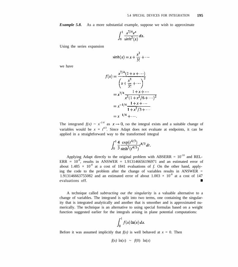
5.4 SPECIAL DEVICES FOR INTEGRATION 195
Example 5.8. As a more substantial example, suppose we wish to approximate
Using the series expansion
we have
The integrand f(x) ~ x-1/4 as so the integral exists and a suitable change ofvariables would be x = t4/3. Since Adapt does not evaluate at endpoints, it can beapplied in a straightforward way to the transformed integral
Applying Adapt directly to the original problem with ABSERR = 10-10 and REL-ERR = 10-8, results in ANSWER = 1.913146656196971 and an estimated error ofabout 1.485 × 10⁻⁸ at a cost of 1841 evaluations of f. On the other hand, apply-ing the code to the problem after the change of variables results in ANSWER =1.913146663755082 and an estimated error of about 1.003 × 10⁻⁸ at a cost of 147evaluations off. n
A technique called subtracting out the singularity is a valuable alternative to achange of variables. The integrand is split into two terms, one containing the singular-ity that is integrated analytically and another that is smoother and is approximated nu-merically. The technique is an alternative to using special formulas based on a weightfunction suggested earlier for the integrals arising in plane potential computations:
Before it was assumed implicitly that f(x) is well behaved at x = 0. Then
f(x) ln(x) ~ f(0) ln(x)
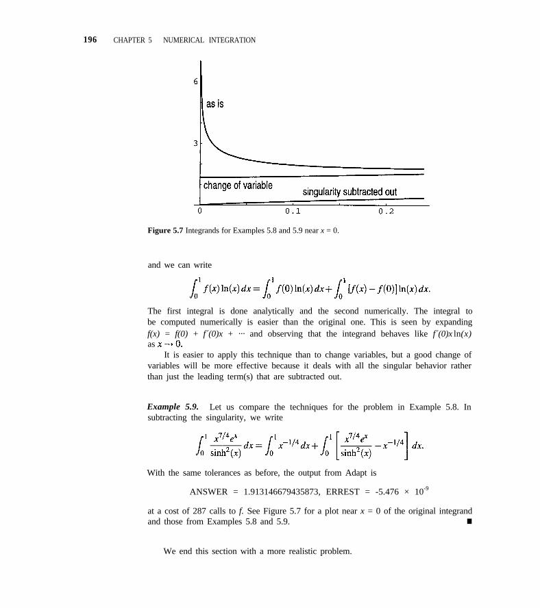
196 CHAPTER 5 NUMERICAL INTEGRATION
Figure 5.7 Integrands for Examples 5.8 and 5.9 near x = 0.
and we can write
The first integral is done analytically and the second numerically. The integral tobe computed numerically is easier than the original one. This is seen by expandingf(x) = f(0) + f´(0)x + ··· and observing that the integrand behaves like f´(0)x ln(x)as
It is easier to apply this technique than to change variables, but a good change ofvariables will be more effective because it deals with all the singular behavior ratherthan just the leading term(s) that are subtracted out.
Example 5.9. Let us compare the techniques for the problem in Example 5.8. Insubtracting the singularity, we write
With the same tolerances as before, the output from Adapt is
ANSWER = 1.913146679435873, ERREST = -5.476 × 10⁻⁹
at a cost of 287 calls to f. See Figure 5.7 for a plot near x = 0 of the original integrandand those from Examples 5.8 and 5.9. n
We end this section with a more realistic problem.
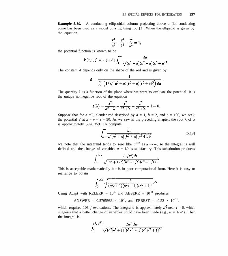
5.4 SPECIAL DEVICES FOR INTEGRATION 197
Example 5.10. A conducting ellipsoidal column projecting above a flat conductingplane has been used as a model of a lightning rod [2]. When the ellipsoid is given bythe equation
the potential function is known to be
The constant A depends only on the shape of the rod and is given by
The quantity λ is a function of the place where we want to evaluate the potential. It isthe unique nonnegative root of the equation
Suppose that for a tall, slender rod described by a = 1, b = 2, and c = 100, we seekthe potential V at x = y = z = 50. As we saw in the preceding chapter, the root λ of φis approximately 5928.359. To compute
(5.19)
we note that the integrand tends to zero like u-5/2 as so the integral is welldefined and the change of variables u = 1/t is satisfactory. This substitution produces
This is acceptable mathematically but is in poor computational form. Here it is easy torearrange to obtain
Using Adapt with RELERR = 10-5 and ABSERR = 10-l4 produces
ANSWER = 0.5705983 × 10⁻⁶, and ERREST = -0.52 × 10⁻¹¹,
which requires 105 f evaluations. The integrand is approximately near t = 0, whichsuggests that a better change of variables could have been made (e.g., u = 1/w2). Thenthe integral is
198 CHAPTER 5 NUMERICAL INTEGRATION
This is a somewhat easier integral to evaluate. Routine Adapt produces
ANSWER = 0.5705883 × 10⁻⁶, and ERREST = 0.46 × 10⁻¹¹,
which requires 35 f evaluations. Note that the two results agree to the requested fivefigures.
These transformations cannot be applied directly to computing A because the in-terval remains infinite. However, since (5.19) has to be computed anyway, we couldsplit
into The first integral is computed to be 0.7218051 × 10⁻⁵ with an errorestimate of 0.31 × 10⁻¹⁰ and requires 357 f evaluations, while the sum using thesecond value from above is 0.7788639 × 10⁻⁵. This yields A = 0.1283921 × 10⁶ andfinally V = -46.3370. n
EXERCISES
Unless otherwise indicated, use as tolerances AB-SERR = 10-8 and RELERR = 10-6 for the comput-ing exercises.
5.13 Evaluate using Adapt
(a) on the problem as is,
(b) using one of the series techniques, and
(c) using a change of variable.
Compare the results.
5.14 Repeat Exercise 5.13 with
5.15 The integral
can be difficult to estimate because of the large num-ber of oscillations as (although the amplitudesare approaching zero, too).
(a) Use Adapt for this problem with RELERR =
Try Adapt with RELERR = 10-2 and ABSERR =½ × 10-3, ½ × 10-6, and ½ × 10-9.
(c) Compare the answers in (a) and (b). Discuss effi-ciency and accuracy.
5.16 The integral
has a rather nasty singularity at x = 0. Analyze thenature of the singularity and argue informally that theintegral exists.
(a) Use Adapt for this problem as it is. How is thiseven possible?
(b) Treat the singularity using a technique from Sec-tion 5.4, then use Adapt.
(c) Compare the answers in (a) and (b). Discuss effi-ciency and accuracy.
10-l2 and the three absolute tolerances ABSERR =10-3, 10-6, and 10-9.
5.17 The exponential integral
(b) The change of variable t = 1/x produces theequivalent integral Approximate thisby where b is chosen sufficiently large.How large should b be in order to guarantee that
t > 0, arises in the study of radiative transfer and trans-port theory [9]. Some manipulation shows that
5.18
5.19
The expression in braces is known to have the value0.5772157, the Euler-Mascheroni constant. The
second term integrates analytically to - lnt. Hence,
Evaluate E1 (t) for t = 1.0, 2.0, 3.0. Does there appearto be any difficulty caused by the behavior of the inte-grand at x = 0?
In studying the conduction properties of a V-groovedheat pipe, a heat flux constant C(θ) satisfies
( θ in radians). Compute values of C for θ = π/6, π/4,π /3, 5π/12, 17π/36. It can be shown mathematicallythat C(θ) is strictly decreasing and 0 < C(θ) < 1. Thedenominator in the integrand vanishes at π/2. Use se-ries expansions to sort out the behavior of the inte-grand at this point, and if it causes difficulty, fix it.
Debye’s specific heat law gives the molar specific heatof a solid, Cv, as a function of its temperature, T:
where R = 1.986 calories/mole is the molar gas con-stant, UD = θD/T, and θD is the Debye temperaturethat is characteristic of each substance. For diamondθD = 1900K, evaluate Cv(T) at the temperatures in-dicated in the accompanying table. Compare with theexperimental values given. Does the behavior of theintegrand at x = 0 appear to cause problems?
5.20
5.4 SPECIAL DEVICES FOR INTEGRATION 199
The Gibb’s effect describes the behavior of a Fourierseries near a discontinuity of the function approxi-mated. The magnitude of the jump can be related tothe integral
which is about 0.281. Routine Adapt cannot be ap-plied directly because it requires a finite interval. Oneway of dealing with this is to drop the tail of the inte-gral, that is, approximate the integral by
This does not work well in this instance because theintegrand decays slowly as To see this, workout an analytical bound for the error made in droppingthe tail, that is, bound
Integration by parts leads to
The integral arising here is easier to approximate be-cause the integrand decays faster. Integration by partscan be repeated to get integrals that are even easierto approximate. Approximate the original integral ac-curately enough to verify that its magnitude is about0.281. Do this by applying Adapt to the integral thatarises after integrating by parts a few times. To ap-ply the code you will have to drop the tail. There aretwo sources of error in the computation. One is theerror made by Adapt, which you can control by thetolerances that you specify. The other error is due todropping the tail. You can control this error by work-ing out an analytical bound for the error and choosinga value b large enough to guarantee the accuracy thatyou need.
200 CHAPTER 5 NUMERICAL INTEGRATION
5.5 INTEGRATION OF TABULAR DATA
The problem addressed here is the approximation of given only (xn,yn) for1 < n < N, where yn = f(xn). Adaptive quadrature routines cannot be used becausethey automatically choose the points where f is to be evaluated and it is unlikely thatsuch points will correspond to the data points {xn}. The basic approach is the same asin Section 5.1: approximate f(x) by a piecewise polynomial function F(x), which isthen integrated exactly.
Since the complete cubic interpolating spline worked so well as an approximatingfunction in Chapter 3, it is a natural choice for F(x). For the sake of simplicity, let usassume that a = x1 and b = xN. Then, using the notation of Chapter 3 for the spline,
Substituting the expressions for an, bn, and dn in terms of the data and cn leads to
(5.20)
An algorithm based on this technique first uses SPCOEF/Spline_coeff from Chapter 3to get and then evaluates (5.20). In terms of h = maxn(xn - xn-1), the com-plete cubic spline S(x) provides an approximation to a smooth function f that is accu-rate to O(h4). Accordingly, if the sample points xi are sufficiently dense in [x1 ,xN] andthe function is sufficiently smooth, we can expect to be an O(h4) estimateof
The cubic spline is familiar and it is easy enough to manipulate once the linearsystem for has been solved, but there are other interesting possibilities. Thelinear system arises because S(x) is required to have two continuous derivatives on[x1 ,xN]. This smoothness is unnecessary to the approximation of Theshape-preserving spline of Section 3.5.2 is less smooth but is attractive here for severalreasons. The reasons and the following formula are left as an exercise:
(5.21)
A widely used scheme is based on local quadratic interpolation. To approximatef(n) by a quadratic over [xn,xn+1 ], we must interpolate it at three points. One possi-

5.5 INTEGRATION OF TABULAR DATA 201
bility is to interpolate at {xn-1 ,xn ,xn+l}. Another is to interpolate at {xn ,xn+1 ,xn+2 } .There is no obvious reason to prefer one to the other and the computation is inexpen-sive, so a reasonable way to proceed is to compute both and average the two results.This provides a symmetrical formula that smooths out mild measurement errors in thetabulated values off. Of course, at the ends n = 1 and n = N - 1, only one quadraticis used. The formula for a typical (interior) interval [xn ,xn+l ] is
(5.22)
Reference [4] contains further discussion and a FORTRAN code AVINT.There is no obvious way to obtain a good estimate of the error of these quadrature
rules, much less to control it. The difficulty is inherent to functions defined solely bytables.
EXERCISES
5.21 In performing an arginine tolerance test, a doctor mea-sures glucose, insulin, glucagon, and growth hormonelevels in the blood over a l-hour time period at 10-minute intervals to obtain the following data:
time glucose insulin0 102 1110 114 2620 122 3630 132 4740 115 39 5.2250 107 2760 100 15 5.23
time glucagon growthhormone
0 188 1.7010 1300 1.7020 2300 1.2030 2600 2.5040 1800 7.2550 840 8.1060 460 8.00
The doctor is interested in the integrated effect of eachresponse. For example, if the glucose curve is repre-sented by g(t), then is desired. Computeone of the integrals by
(a) the method (5.20) based on splines,
(b) the method (5.21) based on splines, and
(c) the method based on averaging quadratics (5.22).
Compare the results.
Supply the details of the derivation of (5.22). Workout the special forms for the end points.
Derive the formula (5.21) for the integration of tabulardata using the shape-preserving spline. When mightyou prefer this to formula (5.20) based on the com-plete cubic spline? Consider the cost of computingthe spline and how well the spline might fit the data.
202 CHAPTER 5 NUMERICAL INTEGRATION
5.6 INTEGRATION IN TWO VARIABLES
Definite integrals in two or more variables are generally much more difficult to approx-imate than those in one variable because the geometry of the region causes trouble. Inthis section we make a few observations about the common case of two variables,especially as it relates to finite elements.
Integration over a rectangle,
can be handled easily with the formulas for one variable by treating I as an iteratedintegral. Thus we first approximate
with one quadrature rule using N1 points {x i} and then
using another rule of N2 points {y j}. This approach generalizes to
It is even possible to use an adaptive code for the integrals in one variable, but thematter is a little complicated. In Fritsch, Kahaner, and Lyness [6] it is explained howto go about this; for pitfalls to be avoided, see [11, Section 9].
Degree of precision now refers to polynomials in two variables, so a formula of,for example, degree 2 must integrate all polynomials of the form
exactly on the region of interest. Just as in the case of one variable, we can derivequadrature formulas by interpolating f(x,y) and integrating the interpolant. This isquite practical for integration over a square or a triangle and is often done. The schemefor rectangles based on iterated integrals can be quite efficient when the formulas forintegration in one variable are Gaussian. They are not necessarily the best that can bedone. As in the one-dimensional case, formulas can be derived that use the smallestnumber of evaluations of f(x,y) to obtain a given degree of precision. Nevertheless,the most efficient formulas may not be the most attractive in practice. The approachbased on interpolation can be very convenient when the interpolation is done at pointsinteresting for other reasons, as in finite elements. The iterated integral approach canbe very convenient because of its simplicity and generality.
In one dimension the transformation of any finite interval [a,b] to a standard onesuch as [-1,l] is trivial. In two dimensions the matter is far more important and
5.7 CASE STUDY 5 203
difficult. Now an integral over a general region R,
must be broken up into pieces that can be transformed into a standard square or trian-gle. Discretizing a region R in this way is an important part of any finite element code.If the region is decomposed into triangles (with straight sides), the easy transformationwas stated in Chapter 3. An integral over a general triangle T becomes an integral overthe standard, reference triangle T*,
Here |D*| is the determinant of the Jacobian of the transformation. It relates the in-finitesimal area dydx in the one set of variables to that in the other set. For the affinetransformation from one triangle (with straight sides) to another, this matter is easy.In the general case it is necessary to investigate whether the transformation is a properone, meaning that the image covers all the triangle T* and has no overlaps.
The main point of this section is that the basic ideas of the one variable casecarry over to several variables. There is the additional and very serious complicationof splitting up the region of integration and transforming properly each piece to astandard region. The whole area of integration of functions of more than one variableis still the subject of research.
EXERCISES
5.24 Given the triangular domain T with vertices (0,0),(1,0), and (01), we would like to approximate
over T.
(a) Derive a quadrature approximation of the form
A 1 f (0, 0) + A2f(0, 1) + A3f(1, 0)
where the coefficients are chosen to make the approx-imation exact for f = 1, x, and y.
(b) Derive a corresponding composite quadrature for-mula for the subdivision obtained by cutting T intofour subtriangles by connecting the midpoints of theedges of T.
5.7 CASE STUDY 5
This case study has two parts, one devoted to a problem involving singular integrandsand the other to problems with integrands that have sharp peaks. As usual, our aim isto understand the difficulties and what might be done to make it possible to solve theproblems effectively with standard codes. The first part is an example of a problemrequiring more than one code for its solution. The second part develops a technique ofclassical applied mathematics and uses it for insight.
Reference [5] discusses the motion of a particle of mass m at position q in a po-tential field V(q). In suitable circumstances the motion is a libration (or oscillation or
204 CHAPTER 5 NUMERICAL INTEGRATION
vibration). For an energy level E, it is found that if the equation E - V(q) = 0 hassimple roots q1 < q2, the period T of the motion is given by
The integrand is singular at both end points, so the first thing we must do is sort out itsbehavior there. Near a simple root qi, a Taylor series expansion tells us that as
hence the singularity is integrable. The argument shows why the theory requires thatthe roots be simple. If qi were a multiple root, say double, the integrand would behavelike
and the integral would not exist. Percival and Richards [5] write, “Gaussian numericalintegration is a very effective method of obtaining the periods of libration in practice.”Gaussian quadrature is generally quite effective, but a crucial point in the present situ-ation is that it can be applied directly because it does not evaluate the integrand at theends of the interval. The formulas of Adapt have the same property.
As a simple example let us take V(q) = (q + l)(q - 0.8)7 and E = -4. As canbe deduced easily from the derivative V´(q) = (8q + 6.2)(q - 0.8)6 or by inspectionof Figure 5.8, V(q) has a minimum at q = -0.775, and for V(-0.775) < E < 0, theequation E - V(q) = 0 has two simple roots, one in [-1, -0.775] and the other in[-0.775,0.8]. To evaluate the integral, we must first compute these roots numerically.The roots should be located very accurately because they define the integral that wewish to approximate. Moreover, if they are not determined accurately, a quadraturecode might evaluate the integrand at an argument q for which the integrand is notdefined because of taking the square root of a negative number or dividing by zero.A problem like this is very easy for Zero, so we take ABSERR = 10-l4 and REL-ERR = 10-14. Even with these stringent tolerances the code requires only 21 functionevaluations to find that -0.9041816 with a residual of about 1.3 × 10-l5 and
-0.5797068 with a residual of about 1.9 × 10⁻¹⁵. Because E provides a naturalmeasure of scale for this equation, the residuals and a backward error analysis make itclear that the roots are very accurate, although of course we already know that becauseZero reported that it had obtained the specified accuracy.
Using the computed values for the end points, it is possible to approximate theintegral by a simple call to Adapt. With ABSERR = 10-6 and RELERR = 10-6 thisresults in an answer of about 0.444687 with an estimated error of about 9.0 × 10⁻⁷ at acost of 3171 function evaluations. This is relatively expensive for Adapt with its (arbi-trary) limit of 3577 evaluations. If we wanted to do a number of integrals of this kind,some preparation of the problem would be worthwhile. We have already worked outthe dominant behavior of the integrand at the end points and the value of the derivativeappearing in the expression is readily available, so the method of subtracting out thesingularity would be easy to apply. However, because the singularity is algebraic, it
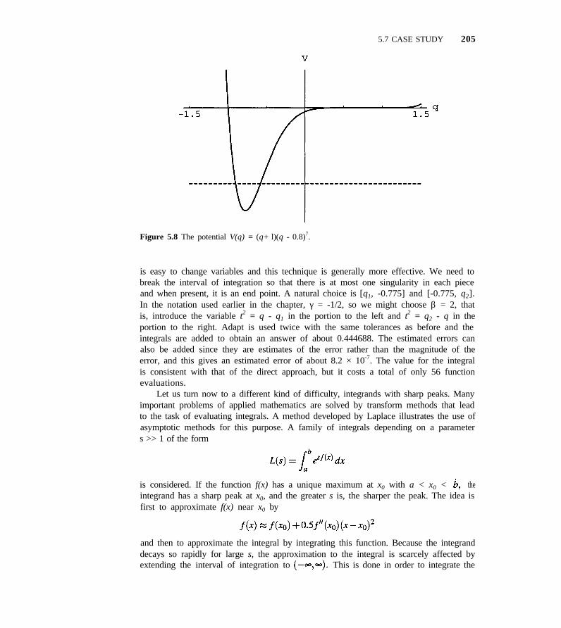
5.7 CASE STUDY 205
Figure 5.8 The potential V(q) = (q+ l)(q - 0.8)7.
is easy to change variables and this technique is generally more effective. We need tobreak the interval of integration so that there is at most one singularity in each pieceand when present, it is an end point. A natural choice is [q1, -0.775] and [-0.775, q2].In the notation used earlier in the chapter, γ = -1/2, so we might choose β = 2, thatis, introduce the variable t2 = q - q1 in the portion to the left and t2 = q2 - q in theportion to the right. Adapt is used twice with the same tolerances as before and theintegrals are added to obtain an answer of about 0.444688. The estimated errors canalso be added since they are estimates of the error rather than the magnitude of theerror, and this gives an estimated error of about 8.2 × 10⁻⁷. The value for the integralis consistent with that of the direct approach, but it costs a total of only 56 functionevaluations.
Let us turn now to a different kind of difficulty, integrands with sharp peaks. Manyimportant problems of applied mathematics are solved by transform methods that leadto the task of evaluating integrals. A method developed by Laplace illustrates the use ofasymptotic methods for this purpose. A family of integrals depending on a parameters >> 1 of the form
is considered. If the function f(x) has a unique maximum at x0 with a < x0 < theintegrand has a sharp peak at x0, and the greater s is, the sharper the peak. The idea isfirst to approximate f(x) near x0 by
and then to approximate the integral by integrating this function. Because the integranddecays so rapidly for large s, the approximation to the integral is scarcely affected byextending the interval of integration to This is done in order to integrate the
206 CHAPTER 5 NUMERICAL INTEGRATION
approximating function analytically. It amounts to approximating the integrand by thefamiliar bell-shaped curve of a normal distribution with mean x0 and standard devia-tion The result of these approximations is Laplace’s formula,
A classic application of this formula is to the Stirling approximation of the gammafunction seen in Example 1.10. Some manipulation of the integral definition of thegamma function puts it into the form required:
(Here t = xs.) Laplace’s formula with f(x) = lnx - x and x0 = 1 then gives
Laplace’s formula and the class of integrals it approximates illustrate how the ap-proximations of classical applied mathematics differ from those of numerical analysis.A general-purpose code like Adapt that accepts any smooth integrand is likely to failwhen presented an integrand with a sharp peak because it is not likely to “see” thepeak. By this we mean that the code is not likely to take samples from the small subin-terval where the peak occurs, so it, in effect, approximates the integrand by a functionthat does not have a peak. The approach of applied mathematics is much less generalbecause it requires that the location of the peak be supplied along with informationabout its width. An advantage of the approach is that it provides important qualitativeinformation about how the integral depends on a parameter. On the other hand, theaccuracy of the formula depends on the parameter, and for a given value of s it mightnot be enough. As is often the case, when used to obtain a numerical approximationto an integral, the approaches are complementary with the one working better as theparameter increases and the other working worse, and vice versa. Let us take advan-tage of the insight provided by Laplace’s method to compute an accurate value foran integral with a sharp peak using a general-purpose code. Clearly we ought first tolocate the peak, then get some information about its width, and finally break up the in-terval appropriately. D. Amos [l] does exactly this to evaluate integral representationsof statistical distributions. In each case an evaluation of the function amounts to thenumerical integration of a bell-shaped integrand with a single maximum at x0. FirstNewton’s method is used to locate x0. A scale σ is then determined using the Laplacemethod. Finally quadratures over intervals of length σ to the left and right of x0 aresummed until a limit of integration is reached or the truncation error is small enough.The basic idea is simple, but the generality of the distributions allowed and the re-finements needed for fast evaluation of the functions make the details too complex todescribe here. To illustrate the approach, we refine the Stirling approximation for thecomputation of a large factorial, a simple example that allows the easy computation ofa reference value.
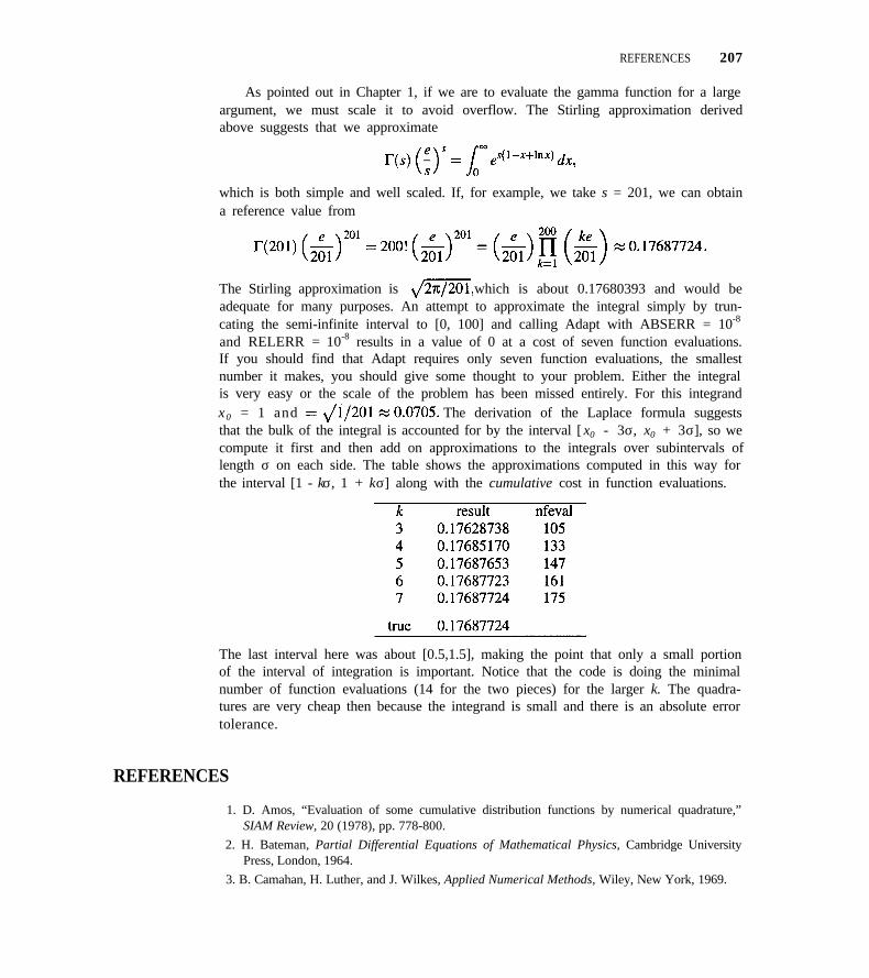
REFERENCES 207
As pointed out in Chapter 1, if we are to evaluate the gamma function for a largeargument, we must scale it to avoid overflow. The Stirling approximation derivedabove suggests that we approximate
which is both simple and well scaled. If, for example, we take s = 201, we can obtaina reference value from
The Stirling approximation is which is about 0.17680393 and would beadequate for many purposes. An attempt to approximate the integral simply by trun-cating the semi-infinite interval to [0, 100] and calling Adapt with ABSERR = 10-8
and RELERR = 10-8 results in a value of 0 at a cost of seven function evaluations.If you should find that Adapt requires only seven function evaluations, the smallestnumber it makes, you should give some thought to your problem. Either the integralis very easy or the scale of the problem has been missed entirely. For this integrandx0 = 1 and The derivation of the Laplace formula suggeststhat the bulk of the integral is accounted for by the interval [ x0 - 3σ, x0 + 3σ], so wecompute it first and then add on approximations to the integrals over subintervals oflength σ on each side. The table shows the approximations computed in this way forthe interval [1 - kσ, 1 + kσ] along with the cumulative cost in function evaluations.
The last interval here was about [0.5,1.5], making the point that only a small portionof the interval of integration is important. Notice that the code is doing the minimalnumber of function evaluations (14 for the two pieces) for the larger k. The quadra-tures are very cheap then because the integrand is small and there is an absolute errortolerance.
REFERENCES
1. D. Amos, “Evaluation of some cumulative distribution functions by numerical quadrature,”SIAM Review, 20 (1978), pp. 778-800.
2. H. Bateman, Partial Differential Equations of Mathematical Physics, Cambridge UniversityPress, London, 1964.
3. B. Camahan, H. Luther, and J. Wilkes, Applied Numerical Methods, Wiley, New York, 1969.
208 CHAPTER 5 NUMERICAL INTEGRATION
4. P. Davis and P. Rabinowitz, Methods of Numerical Integration, 2nd ed., Academic Press, NewYork, 1984.
5. I. Percival and D. Richards, Introduction to Dynamics, Cambridge University Press, Cambridge,Mass., 1982.
6. F. Fritsch, D. Kahaner, and J. Lyness, “Double integration using one-dimensional adaptivequadrature routines: A software interface problem,” ACM Trans. on Math. Software, 7 (1981),pp. 46-75.
7. Handbook of Mathematical Functions, M. Abramowitz and I. Stegun, eds., Dover, Mineola,N.Y., 1964.
8. E. Issacson and H. Keller, Analysis of Numerical Methods, Dover, Mineola, N.Y., 1994.
9. V. Kourganoff, Basic Methods in Transfer Problems, Relative Equilibrium and Newton Dim-sion, Dover, New York, 1963.
10. A. Kronrod, Nodes and Weights of Quadrature Formulas, (Trans.) Consultants Bureau, NewYork, 1965.
11. J. Lyness, “When not to use an automatic quadrature routine,” SIAM Review, 25 (1983), pp. 63-87.
12. R. Piessens, E. de Doncker-Kapenga, C. Überhuber, and D. Kahaner, QUADPACK: SubroutinePackage for Automatic Integration, Springer-Verlag, New York, 1983.
13. A. Stroud and D. Secrest, Gaussian Quadrature Formulas, Prentice Hall, Englewood Cliffs,N.J., 1966.
EXERCISES
Unless otherwise indicated, use ABSERR = 10-8 andRELERR = 10-6 for the computing exercises.
5.25 The potential inside the unit circle due to a specifiedpotential f(θ) on the boundary is given by Poisson’sintegral:
There is difficulty evaluating this integral assince for θ´ = θ,
This is not too severe because the term is large onlyif r is very close to 1, but in principle there should beno difficulty at all since asBateman [2, pp. 239-241]). Realizing that
and argue that it should have somewhat better numer-ical properties. Explore this by evaluating φ(r,θ) for rapproaching 1 with f(θ) = sinθ. The analytical solu-tion is then just ϕ(r, θ) = rsinθ.
5.26 The potential in a conducting strip of width b withpotential zero on the bottom edge and a specified po-tential F(x) on the upper edge is
where β = πy/b. Suppose that an experimenter ap-plies the potential F(x) = 1 for |x| < 0.99 and F(x) =exp[- 100( |x| - 0.99)] for |x| > 0.99. When b = π,compute and plot the potential along the middle of thestrip, ψ(x, π/2).
Realizing that
bound the effect on ϕ(x,y) for y 0 of replacing thederive the form infinite interval by a finite one:
For a suitable choice of z, use this instead of the infi- 5.28nite interval. Show for the given F(x) that ϕ(x,y) =ϕ(-x,y), so only a plot for x > 0 is necessary.
5.27 This exercise is representative of a great many com-putations arising in the use of the classical separa-tion of variables technique for solving field problems.Typically, one must compute many roots of nonlinearequations and integrals. The temperature distributionin a cylinder of radius a and height b with the bottomheld at a temperature zero, the top at a temperaturef(r), and the side dissipating heat according to New- 5.29ton’s law of cooling, can be represented by a series.If the thermal conductivity of the cylinder is k and thethalpance is ε, then the temperature ϕ(r,z) is
The numbers qn are the positive roots of the equation
where the function J0(x) and J1(x) are Bessel func-tions of the first kind of orders zero and one, respec-tively. The coefficients An are given by
The roots qn depend only on the geometry and the ma-terial. Once they have been computed, one can con-sider virtually any temperature distribution f(r) by 5.30computing the quantities An. For k/ε a = 2, we givethe problem of solving for qna for n = 1, 2, 3 in Ex-ercise 4.18. If you have not done that problem, theroots are 0.940770563949734, 3.95937118501253,and 7.08638084796766. Then for a = 1, computeA1, A2, A3 for f(r) = exp(-r) - exp(-1).
Miscellaneous Exercises 209
If 6 what is C? To answer this,apply Zero with modest tolerances to compute the root
C of f(C) = 6 Evaluate the in-tegral appearing in the function with Adapt and morestringent tolerances. A little analysis will provide anappropriate bracket to use for the root solver. Showanalytically that the root is simple. This is an exam-ple of computing the roots of a function that is rela-tively expensive to evaluate. How many evaluationsdid Zero need?
Reference [3] contains the following problem. Thelength L of a carbon dioxide heat exchanger with in-put temperature T1 and output T0 satisfies
where m = 22.5, D = 0.495, Ts = 550 (temperature ofthe CO2),
For T1 = 60, and L = 10, use Adapt and Zero to com-pute T0.
The code Adapt uses a queue to hold the subinter-vals whose quadrature errors are deemed too large topass the tolerance test. Do you think there would beany difference in performance if a stack were used in-stead? Explain. Modify Adapt so that it uses a stackand test it on some difficult problems to see what ac-tually happens.
CHAPTER 6
ORDINARY DIFFERENTIALEQUATIONS
Historically, ordinary differential equations have originated in chemistry, physics, andengineering. They still do, but nowadays they also originate in medicine, biology,anthropology, and the like. Because differential equations are more complex theoreti-cally than the other topics taken up in this book and because their numerical solutionis less well understood, the art of numerical computing plays an important role in thischapter. There is a subdiscipline of numerical analysis called mathematical softwarethat colors all the work of this book. It is particularly evident in this chapter with itsmore complex task.
6.1 SOME ELEMENTS OF THE THEORY
The simplest kind of ordinary differential equation problem is to find a function y(x)with a derivative continuous on [a,b] such that
y´(x) = f(x), a < x < b,
for a given continuous function f(x). From elementary calculus it is known that such afunction y(x) exists—the indefinite integral of f(x). However, if y(x) satisfies the dif-ferential equation, so does y(x) + c for any constant c. To specify a particular solution,some more information about y(x) is required. The most common kind of additionalinformation supplied is the value A of y(x) at the initial point a. Then
is the unique solution to the initial value problem consisting of the differential equationsatisfied by y(x) and the initial value of y(x).
The general first order ordinary differential equation has f depending on y as wellas x. It is assumed that f(x,y) is continuous for a < x < b and all y. A solution y(x) isa function of x with a continuous derivative for a < x < b that satisfies the equation
y´(x) = f(x,y(x)) (6.1)
210
6.1 SOME ELEMENTS OF THE THEORY 211
for each x in the interval [a,b]. Typically the solution desired is specified by its valueat the initial point of the interval:
y(a) = A. (6.2)
Equation (6.2) is called an initial condition, and the combination of (6.1) and (6.2) iscalled an initial value problem for an ordinary differential equation.
In elementary treatments of differential equations, the initial value problem has aunique solution that exists throughout the interval of interest and that can be obtainedby analytical means (more familiarly called a “trick”). However, for most problemsthat are not contrived, an analytical solution is impossible to obtain or is less satisfac-tory than a numerical solution. Matters are also complicated by the fact that solutionscan fail to exist over the desired interval of interest. Problems with solutions that“blow up” place a special burden on a numerical procedure, although we might wellexpect a general-purpose code to compute such solutions until overflow occurs. Prob-lems that have more than one solution are especially troublesome. Difficulties withexistence and uniqueness will be excluded at the level of the theory to be developedhere. A simple condition that guarantees that these difficulties will not occur can beformulated in terms of how f(x,y) depends on y.
The function f(x,y) satisfies a Lipschitz condition in y if for all x in the interval[a,b] and for all u, v,
with L a constant, hereafter called a Lipschitz constant. The inequality assumes a morefamiliar form if f has a continuous partial derivative in its second variable, for then
for some w between u and v. If is bounded in magnitude for all arguments, thenf satisfies a Lipschitz condition and any constant L such that
for all x in [a,b] and all w is a Lipschitz constant. If the partial derivative is notbounded, it is not hard to show that the inequality (6.3) cannot hold for all u, v and allx in [a,b], so f does not satisfy a Lipschitz condition.
Example 6.1. The function f(x,y) = x2 cos2 y + y sin2x defined for |x| < 1 and ally satisfies a Lipschitz condition with constant L = 3. To see this, differentiate withrespect to y to get
and so for the range of x allowed
n
212 CHAPTER 6 ORDINARY DIFFERENTIAL EQUATIONS
Example 4.2. The function f(x,y) does not satisfy a Lipschitz conditionbecause it has a continuous partial derivative for y > 0 that is not bounded as
An important special case of (6.1) is that of a linear differential equation, an equa-tion of the form f(x,y) = g(x)y + h(x). The function f(x,y) being continuous in (x,y)is then equivalent to g(x) and h(x) being continuous in x. Because
and because a continuous function g(x) is bounded in magnitude on any finite interval[a,b], a linear equation is Lipschitzian in nearly all cases of practical interest.
Example 6.3. Dawson’s integral is the function
You should verify that it is a solution of the initial value problem for the linear differ-ential equation
y´ = l - 2x y
y(0) = 0.
On the interval [0,b] for any b 0, the function f(x,y) = 1 - 2 xy is continuous andLipschitzian with Lipschitz constant L = 2|b|. n
Sufficient conditions for existence and uniqueness can now be stated formally. Fora proof, see [3].
Theorem 6.1. Let f(x,y) be continuous for all x in the finite interval [a,b] andall y and satisfy (6.3). Then for any number A, the initial value problem y´ = f(x,y),y(a) = A has a unique solution y(x) that is defined for all x in [a,b].
So far we have spoken of a single equation in a single unknown y(x). More com-monly there are several unknowns. By a system of m first order differential equationsin m unknowns is meant
(6.4)
6.1 SOME ELEMENTS OF THE THEORY 213
Along with the equations (6.4) there are initial conditions
Y1(a) = A1
Y2(a) = A2
( 6 . 5 )
then (6.4) and (6.5) become
Ym(a) = Am.
This can be written in tidy fashion using vector notation. If we let
Y´ = F(x, Y)
Y(a) = A.
(6.6)
(6.7)
We again refer to the combination of (6.4) and (6.5) as an initial value problem. Usingvector notation makes the case of m unknowns look like the case of one unknown. Oneof the fortunate aspects of the theory of the initial value problem is that the theory fora system of m first order equations is essentially the same as for a single one. Proofsfor systems just introduce vectors and their norms where there are scalars and absolutevalues in the proofs for a single equation. For the vector function F( x,Y) to satisfya Lipschitz condition, it is sufficient that each Fi (x, Y1, Y2,. . . , Ym) satisfy a Lipschitzcondition with respect to each variable Yj; that is, there are constants Lij such that
for each i, j. With this, the natural analog of Theorem 6.1 holds. Since the theory ofnumerical methods for a system of equations is also essentially the same as for a singleequation, we content ourselves with treating the case of a single equation in detail andjust state the analog for systems.
Most computer codes require the problem to be provided in the standard form(6.4) and (6.5), but equations arise in a great variety of forms. For example, secondorder equations, that is, equations of the form
y´´ = g(x,y,y´),
are quite common in the context of dynamical systems. The definition of a solu-tion is the obvious extension of the first order case and suitable initial conditions arey(a) = A1, y´(a) = A2. This is a second order equation for one unknown quantity, y(x).An equivalent problem in the standard form (6.4) can be found by introducing twounknown quantities and finding two first order equations satisfied by them. One of thenew unknowns has to provide us with the original unknown, so we take Y1(x) = y(x).
214 CHAPTER 6 ORDINARY DIFFERENTIAL EQUATIONS
We take the other unknown to be the derivative of the original unknown, Y2(x) = y´(x).Differentiating the new unknown quantities, we find that
Y´1 = y´(x) = Y2(x),
Y´2 = y´´(x) = g(x,y(x),y´(x)) = g(x,Y1(x),Y2(x)).
In this way we come to the system of two first order equations in two unknowns:
Y´1 = Y2
Y´2 = g(x,Y1,Y2).
This is in standard form and the theory may be applied to it to conclude the existenceof unique functions Y1(x) and Y2(x) that satisfy initial conditions
Y1(a) = A1
Y2(a) = A2.
The solution of the original problem is obtained from y(x) = Y1(x). To verify this, firstnotice that one of the equations states that y´(x) = Y´1(x) = Y2(x), and the other that
y´´(x) = Y´2(x) = g(x,Y1(x),Y2(x)) = g(x,y(x),y´(x)).
Similarly it is found that the initial conditions are satisfied.The general mth order equation in one unknown,
y(m) = g(x, y, y´, . . . , y(m-1)
y(a) = A1,y´(a) = A2,. . . , y(m-1) = Am,
can be put into standard form via the m unknowns Y1(x) = y(x), Y2(x) = y´(x), . . .,Ym(x) = y(m-l)(x) and
Example 6.4. To convert the initial value problem
y´´ + (y2- l)y´ + y = 0, y(0) = 1, y´(0) = 4
into a system of first order equations, let
Y1(x) = y(x), Y2(x) = y´(x)
Then
Y´1 = y´ = Y2
Y´2 = y´´ = -(Y21 - l)Y2 - Y1
6.1 SOME ELEMENTS OF THE THEORY 215
and
Y1(0) = 1, Y2(0) = 4.
This can be put into the form (6.7) by defining
Example 6.5. Consider the system of second order equations
Let Y1(x) = u(x), Y2(x) = u´(x), Y3(x) = v(x), and Y4(x) = v´(x). Then the equationsare
Y´2 + 5Y4 + 7Y1 = sinx, Y´4 + 6Y4 + 4Y2 + 3Y1 + Y3 = cosx,
which is rearranged as
with initial conditions
Y 1(0) = 1, Y2(0) = 2, Y3(0) = 3, Y4(0) = 4.
To put this into the form (6.7) define
and
Notice that for each unknown in the original set of equations, new unknowns are in-troduced for the original unknown and each of its derivatives up to an order one lessthan the highest appearing in the original set of equations. n
The procedure we have illustrated is the usual way to convert a system of higherorder equations to a system of first order equations. There are, however, other ways todo it. For some examples, see Exercise 6.6.
216 CHAPTER 6 ORDINARY DIFFERENTIAL EQUATIONS
EXERCISES
6.1 As an example of nonuniqueness of solutions, verifythat for any constant c, 0 < c < b, the function y(x)defined by
is a solution of the initial value problem
6.2 Consider the problem
Verify that
(a) y(x) = 1 is a solution on any interval containingx = 0,
(b) y(x) = coshx is a solution on [0,b] for any b > 0,and
(c) y(x) = cosx is a solution on a suitable interval.What is the largest interval containing x = 0 on whichcosx is a solution?
6.3 Verify the statement in the text that Dawson’s integralis a solution of the initial value problem
y´ = l - 2x y
y (0) = 0.
6.4 For each initial value problem, verify that the giveny(x) is a solution.
(d) y´ = 100(sinx - y) , y(0) = 0;y(x) = [102(e-100x -cosx) + 104 sin x]/(104 + 1)
6.5 Do the following functions satisfy a Lipschitz condi-tion? If so, give suitable constants.
(a) f(x,y) = 1 + y2 for 0 < x π/2
(b) f(x,y) = 1 - 2xy for 0 < x < b
(c) f(x,y) = y/x for 1 < x < 2
(d) f(x,y) = y/x for -1 < x < 1
(e) f(x,y) = cosx siny for -106 < x < 106
6.6 Verify for each of the following systems of equations
(a) Y´1 = Y2, Y´2 = -x2Y1 - xY2
(b) Y´1 =
(c) Y´1 = -(x/2)Y1 + Y2, Y´2 = (1/2 - 3x 2/4)Y1 -( x / 2 )Y 2
that Y1(x) = y(x), where y(x) satisfies the second orderequation
y´´(x) + xy´(x) + x2y(x) = 0.
6.7 Put the following problems in standard form. Differ-entiation is with respect to t.
(a) u(4) + etu´ - tu = cos αt
(b) u´´ + v´ cost + u = t,v´ + u´ + v = et
(c) u´´ + 3v´ + 4u + v = 8t,u´´ - v´ + u + v = cost
(d) mx´´ = X(t, x, y, z, x´, y´, z´),my´´ = Y(t, x, y, z, x´, y´, z´),mz´´ = Z(t, x, y, z, x´, y´, z´)
(e) u(6) + uu´ = et
6.2 A SIMPLE NUMERICAL SCHEME
Let us again consider the initial value problem (6.1) and (6.2),
y ́ = f(X,Y)
y(a) = A,
on the interval [a,b]. The numerical methods we consider generate a table of approx-imate values for y(x). For the moment we suppose that the entries are for equally
6.2 A SIMPLE NUMERICAL SCHEME 217
spaced arguments in x. That is, we choose an integer N and for h = (b - a) /N, weconstruct approximations at the points xn = a + nh for n = 0, 1, . . . , N. The notationy(xn) is used for the solution of (6.1) and (6.2) evaluated at x = xn, and yn is used foran approximation to y(xn).
A differential equation has no “memory.” If we know the value y(xn), Theorem 6.1applies to the problem
u´ = f(x,u)
u(xn) = y(xn)
and says that the solution of this initial value problem on the interval [xn,b] is justy(x). [After all, y(x) is a solution and the theorem says there is only one.] That is, thevalues of y(x) for x prior to x = xn, do not directly affect the solution of the differentialequation for x after xn. Some numerical methods have memory and some do not. Theclass of methods known as one-step methods have no memory—given yn, there is arecipe for the value yn + 1 that depends only on xn, yn, f, and h. Starting with the obviousinitial value y0 = A, a one-step method generates a table for y(x) by repeatedly takingone step in x of length h to generate successively y1, x2, . . . .
The simplest example of a one-step method is Euler’s method. We study it becausethe details do not obscure the ideas and the general case is much the same. A Taylorseries expansion of y(x) about x = x, gives
with xn < ξn < xn+1, provided that y(x) Using the fact that y(x) satisfies(6.1), this is
For small h,
(6.8)
This relation suggests
Euler’s method:
y0 = A
yn+l = yn + hf(xn,yn), n = 0, 1, . . . , N - 1. (6.9)
Example 6.6. Tabulate Dawson’s integral on [0, 0.5] using Euler’s scheme with h =0.1. Recall from Example 6.3 that Dawson’s integral is the solution of the initial valueproblem
y´ = 1 - 2xy
y(0) = 0.
218 CHAPTER 6 ORDINARY DIFFERENTIAL EQUATIONS
Taking y0 = 0, we see that
y1 = 0 + 0.1 × (1 - 2 × 0 × 0) = 0.l;
similarly,
y2 = 0.1 + 0.l × (1 - 2 × 0.1 × 0.1) = 0.198.
Continuing in this manner, the following table results. The true values of the integraly(xn) are taken from [7].
To study the convergence of Euler’s method, we relate the error at xn+1 to the errorat xn. Subtracting (6.9) from (6.8) gives
Denoting the error at xn by En = y(xn) - yn, the Lipschitz condition on f and thisequation imply that
With the definition
we obtain
(6.10)
Here the term h2M2/2 bounds the error made in the current step and the other termbounds the error propagated from preceding steps.
To prove convergence, we bound the worst error that can arise as we step fromx0 = a to xN = b and then show that it tends to zero as h does. The first order ofbusiness is to see how rapidly the inequality (6.10) allows the error to grow. To do thiswe establish a general result for later use. Suppose there are numbers δ > 0 and M > 0such that the sequence d0, d1 , . . . satisfies
6.2 A SIMPLE NUMERICAL SCHEME 219
The case n = 0,
d1 < (1 + δ)d0 + M,
can be combined with the case n = 1 to obtain
d2 < (l + δ)dl + M < (1 + δ) 2d0 + M[1 + (1 + δ)].
Similarly,
d 3 < ( l + δ )d2 + M < (1 + d)3d0 + M[1 + (1 + δ) + (1 + δ)2].
At this point we might guess that
dn < (1 + δ) n d0 + M[1 + (1 + δ) + (1 + δ)2+ ··· +(1 + δ)n-1]. (6.11)
To prove this, we use induction. The inequality (6.11) certainly holds for n = 1, 2, 3.Suppose the inequality is true for the case n = k. Then
dk + 1 < (1 + δ)dk + M
< (1 + δ)k+1 d0 + M[1 + (1 + δ) + ··· + (1 + δ)k],
which establishes the result for n = k + 1 and completes the induction argument.
Lemma 6.1. Suppose there are numbers δ > 0 and M > 0 such that the sequenced0, d1 , . . . satisfies
dk+l < (l + δ) dk + M, k = 0, l, . . . .
Then for any n > 0,
(6.12)
Proof. Using the identity
with x = 1 + δ, we see that the right-hand side of (6.11) can be rewritten in the form
(6.13)
Expansion of the exponential function about zero gives for δ > 0,
It then follows that
and
220 CHAPTER 6 ORDINARY DIFFERENTIAL EQUATIONS
This implies that (6.13) is bounded by
which establishes (6.12). n
Returning now to Euler’s method, we apply Lemma 6.1 to (6.10) and arrive at
However, nh = xn - a and E0 = y0 - A = 0, so
(6.14)
Using xn - a < b - a, this implies that
(6.15)
It is seen that the error of Euler’s method is bounded by a constant times h. When thevalue of the constant is immaterial, such expressions are written as 0(h).
Generally speaking, we try to ignore the effects of finite precision arithmetic.When the tolerance corresponds to a relative accuracy comparable to the word lengthof the computer, this is not possible. Also, if the solution is very hard to approximateaccurately at xn, the step size necessary may be so small that the precision must beconsidered. To gain some insight, note that we do not obtain f(xn,yn) from a subrou-tine, but rather f(xn,yn) + εn. Similarly, in computing yn+1 = yn + h[ f(xn,yn) + εn] madditional error ρn is made. The sequence generated computationally is then
yn+l = yn + hf(xn,yn) + hεn + ρn .
Let us suppose that |ρn| < ρ and |ρn| < ε for all h < h0. Then the analysis can bemodified to yield
According to this bound, roundoff effects get worse as the step size is reduced inan attempt to get a more accurate solution. Clearly there is a maximum accuracypossible that depends on the problem, the numerical method, and the arithmetic of thecomputer used. The effects are more complex than this bound shows, but the boundis qualitatively correct. It is easy to show experimentally that as h is decreased, thenumerical solution is at first more accurate, reaches a best value, and subsequently isincreasingly less accurate.
The convergence analysis just presented is the traditional one. The trouble is thatthis is not the way modern codes work. Rather than take a step of specified lengthh, they select a step size automatically that will produce a solution with a specifiedaccuracy. A reasonable model of the step sizes selected by such codes is that at xn
the code selects a step hn where is a piecewise-continuous function
6.3 ONE-STEP METHODS 221
satisfying 0 < q < < 1 for a < x < b. With this model it is easy enough to modifythe convergence proof just given to account for variable step size. The result is that asthe maximum step size H tends to zero, It is not hardto see how the model comes about. The user specifies a tolerance τ. In a step of lengthh from xn, Euler’s method makes an error of approximately h2|y´´(xn)|/2. The largeststep size hn that can be used and still keep the error less than τ is then about
Special rules come into play in the codes when y´´(xn,) is nearly zero, so suppose thaty´´(x) does not vanish in [a,b]. If
and
then
defines Notice that H = O(τ 1/2) so that max |y(xn) - yn| is O(τ 1/2) for Euler’smethod with automatic selection of the step size.
EXERCISES
6.8 Use Euler’s method on the following problems using 6.9 Implement Euler’s method to estimate solutions of thea fixed step size h = 1.0, and then h = 0.5. In each initial value problem in Exercise 6.8b. Use h = l/40case calculate the errors at x = 1.0. and h = l/80. Compute the errors at x = 0.5 and
(a) y´ = -y/ ( x + 1) with y(0) = 1, so y(x) = l/(x + x = 1.0 to see if they are roughly halved as h is. How
1).small an h would you estimate is needed in order for
(b) y´ = -y3/2 with y(0) = 1, so y(x) the absolute error to be less than 10-6 in magnitude?
6.3 ONE-STEP METHODS
Let us now consider general one-step methods and base our assumptions on the suc-cessful treatment of Euler’s method. The recipe is to be of the form
y0 = A(6.16)
222 CHAPTER 6 ORDINARY DIFFERENTIAL EQUATIONS
The method has no memory, so Φ depends only on the arguments listed. Usually fand h are omitted in the notation. It is assumed that Φ is continuous in x and y. Thetreatment of Euler’s method had Φ(x,y) = f(x,y) and a Lipschitz condition was usedin an important way. So, for the general procedure we assume that
(6.17)
for a < x < b, all 0 < h < h0 for some h0, any continuous function f satisfying aLipschitz condition, and all u, v.
In discussing Euler’s method we used as a starting point the fact that the solutiony(x) almost satisfies the recipe (6.9) used to define the numerical approximation. Theanalog here is
(6.18)
with µn “small.” More precisely, if for all xn in [a,b] and all h < h0, there are constantsC and p such that
(6.19)
then we say that the method is of order p for the equation (6.1). The quantity µn iscalled the local truncation error.
Theorem 6.2. Suppose the initial value problem
y´ = f(x,y)
y(a) = A
on the finite interval [a,b] is solved by the one-step method (6.16) and suppose that thehypotheses of Theorem 6.1 are satisfied. If Φ(x,y) satisfies (6.17) and if the method isof order p > 1 for y(x), then for any xn = a + nh [a,b],
Proof As before, let En = y(xn) - yn and subtract (6.16) from (6.18) to obtain
Using the Lipschitz condition (6.17) and the fact that the method is of order p, we seethat
The theorem now follows from Lemma 6.1 and the fact that E0 = 0. n
As with our discussion of Euler’s method, the result of this theorem gives conver-gence of O(hP). This explains our calling the method of order p for y(x). The term “amethod of order p´´ is used to describe a method that is of order p if f is sufficientlysmooth. The order of convergence is lower when f is not so smooth.
As explained in connection with Euler’s method, codes select the step size auto-matically so as to keep the error smaller than a tolerance τ at each step. At the same
6.3 ONE-STEP METHODS 223
time they try to use an efficiently large step. A reasonable model of such a step sizealgorithm leads to a step size hn at xn given by
for a piecewise-continuous function Θ(x) with 0 < θ < Θ(x) < 1 on [a,b] With stepsizes specified in this way, the convergence proof can be altered easily to conclude thatthe error is O(HP) = 0(τ1 / P ) .
The most important task now left is to find functions Φ that are inexpensive toevaluate and of order p for smooth f. We need, then,
with µn = O(hp). A Taylor series expansion of y(x) shows that
if y(x) So we find that if the method is of order p, then it must be thecase that
with z(x) = O(hP). Because y(x) is a solution of the differential equation y´(x) =
f(x,y(x)), the derivatives of y can be expressed in terms of total derivatives of f.Using the notation f(m) (x,y(x)) for the mth total derivative of f and subscripts forpartial derivatives, the relation is
y(m)(x) = f(m-1) (x,y(x)),
where
The expression for Φ(x,y) becomes
(6.20)
An obvious choice for Φ is the function T(x,y),
which yields a family of one-step methods called the Taylor series methods. Euler’smethod is the case p = 1. When it is possible to evaluate derivatives efficiently, thesemethods are very effective.
224 CHAPTER 6 ORDINARY DIFFERENTIAL EQUATIONS
For a simple equation like that satisfied by Dawson’s integral, and especially whenhigh accuracy is desired, a Taylor series method may be the best way to proceed. Thisequation has
f(x,y) = 1 - 2xy
f(1)(x,y) = -2.x + (4x2 - 2)y,
and so forth. Exercise 6.13 develops a simple recursion that makes it easy to use aTaylor series method of very high order for this equation.
Runge-Kutta methods use several evaluations of f(x,y) in a linear combination toapproximate y(x). The simplest case is Euler’s method that uses one evaluation. Letus now derive a procedure using the two evaluations f(xn,yn) and f(xn + p1h,yn +p2hf(xn,yn)), where p1 and p2 are parameters. Then for Φ we use the linear combi-nation R(x,y):
R(xn,yn) = a1f(xn,yn) + a2f(xn + p1h,yn + p2hf(xn,yn)).
In this expression we are free to choose any useful values for p1, p2, a1, and a2. Theaim is to choose the parameters so that the representation (6.19) holds for as large avalue of p as possible. To carry this out we expand all the quantities in Taylor seriesin h and equate coefficients of like powers. To simplify the notation, arguments areshown only if they are different from (xn,yn). The reader familiar with Taylor seriesexpansions of a function of two variables may skip to the result. Otherwise, we canproceed by a succession of familiar one-variable expansions as follows:
Now we want to choose the parameters so that
or, writing this out,
6.3 ONE-STEP METHODS 225
Equating terms involving the same powers of h, it is found that it is possible to obtainagreement only for h0 and h1 :
h0 : a1 + a2 = 1
h1 : a2p2 = ½
a2p1 = ½.
Let a2 = α. Then for any value of the parameter α,
a2 = α
a1 = 1 - α
gives a formula with agreement in all terms involving h0. If we further require thatthe choice
gives a formula with agreement in all terms involving h1. Then
yields a family of one-step methods of order 2 when and f is sufficiently smooth.Some of the members of this family of formulas have names. Euler’s method
has α = 0 and the order p = 1. Heun’s method (the improved Euler method) is thecase α = l/2, and the midpoint or modified Euler method is the case α = 1. The broadapplicability of these formulas is seen when we ask what is needed for the convergencetheorem to be valid. The continuity of R obviously follows from that of f. It is apleasant fact that the Lipschitz condition on R also follows from that on f:
for all 0 < h < h0, and we may take the Lipschitz constant for R to be
226 CHAPTER 6 ORDINARY DIFFERENTIAL EQUATIONS
Therefore, if the differential equation satisfies the conditions of Theorem 6.1, and if thefunction f has two continuous derivatives [which implies the solutionany member of the family with is convergent of order 2.
Higher order procedures involving more substitutions can be derived in the sameway, although naturally the expansions become (very) tedious. As it happens, p evalu-ations off per step lead to procedures of order p for p = 1, 2, 3, 4 but not for 5. For thisreason, fourth order formulas were often preferred for constant step size integrations.As in the second order case, there is a family of fourth order procedures depending onseveral parameters. The classical choice of parameters leads to the algorithm
y0 = A,
and for n = 0, l, . . . ,
This is formulated for the first order system of equations
Y(a) = A
Y´ = F(x,Y)
in a natural way:
Y0 = A,
and for n = 0, l, . . . ,
the classical Runge-Kutta algorithm is
6.3 ONE-STEP METHODS 227
Another quite similar fourth order procedure is
(6.21)
There is little reason to prefer one of these procedures over the other as far as a singlestep is concerned. In the next section we shall learn how R. England exploited (6.21)to achieve an estimate of the error made in the step.
EXERCISES
6.10
6.11
6.12
A definite integral can be evaluated by solv-ing an initial value problem for an ordinary differentialequation. Let y(x) be the solution of
y´ = f(x), a < x < b
y(a) = 0.
Then
Runge-Kutta methods integrate the more generalequation y´ = f(x,y). In this special case, they assumeforms familiar in quadrature. Referring to Chapter 5,identify the familiar procedure to which both the clas-sical fourth order formula and England’s formula de-generate.
Implement Heun’s method to estimate the solutionof the initial value problem in Exercise 6.8b. Useh = 1/40 and h = 1/80. Compute the errors at x = 0.5and x = 1.0 to see if they are roughly quartered as h ishalved. How small an h would you estimate is neededin order for the absolute error to be less than 10-6 inmagnitude?
Implement the classical Runge-Kutta algorithm to es-timate the solution of the initial value problem in Ex-ercise 6.8b. Use h = 1/40 and h = 1/80. Computethe errors at x = 0.5 and x = 1.0. By what factor arethe errors reduced as h is halved? Roughly speaking,
what is the largest value of h for which the absoluteerror will be less than 10-6 in magnitude?
6.13 Consider the linear equation
y´ = P1(x)y + Q1(x).
Show that the derivatives needed in Taylor seriesmethods can be obtained from
y(r) = Pr(x)y + Qr(x),
where
Pr(x) = P´r-1(x) + P1(x)Pr-1(x)
Qr(x) = Q´r-1(x) + Q1(x)Pr-1(x), r = 2, 3, . . . .
Use this to develop a fifth order formula for comput-ing Dawson’s integral.
6.14 An interesting fact about Runge-Kutta methods is thatthe error depends on the form of the equation as wellas on the solution itself. To see an example of this,show that y(x) = (x + 1)2 is the solution of each of thetwo problems
y´ = 2(x + 1), y(0) = 1y´ = 2y/(x + 1), y(0) = 1.
Then show that Heun’s method is exact for the firstequation. Prove that the method is not exact when ap-plied to the second equation, although it has the samesolution.
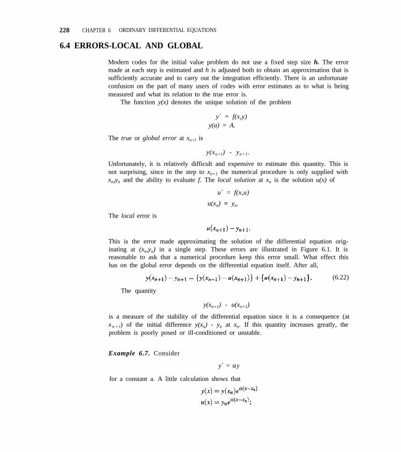
228 CHAPTER 6 ORDINARY DIFFERENTIAL EQUATIONS
6.4 ERRORS-LOCAL AND GLOBAL
Modern codes for the initial value problem do not use a fixed step size h. The errormade at each step is estimated and h is adjusted both to obtain an approximation that issufficiently accurate and to carry out the integration efficiently. There is an unfortunateconfusion on the part of many users of codes with error estimates as to what is beingmeasured and what its relation to the true error is.
The function y(x) denotes the unique solution of the problem
y´ = f(x,y)y(a) = A.
The true or global error at xn+l is
y(xn+l) - yn+1.
Unfortunately, it is relatively difficult and expensive to estimate this quantity. This isnot surprising, since in the step to xn+1 the numerical procedure is only supplied withxn,yn and the ability to evaluate f. The local solution at xn is the solution u(x) of
u´ = f(x,u)
u(xn) = yn.
The local error is
This is the error made approximating the solution of the differential equation orig-inating at (xn,yn) in a single step. These errors are illustrated in Figure 6.1. It isreasonable to ask that a numerical procedure keep this error small. What effect thishas on the global error depends on the differential equation itself. After all,
(6.22)
The quantity
y(xn+1) - u(xn+1)
is a measure of the stability of the differential equation since it is a consequence (atx n + l) of the initial difference y(xn) - yn at xn. If this quantity increases greatly, theproblem is poorly posed or ill-conditioned or unstable.
Example 6.7. Consider
y´ = αy
for a constant a. A little calculation shows that
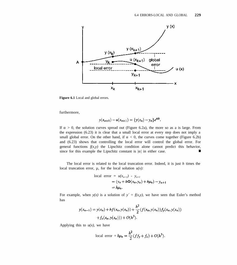
6.4 ERRORS-LOCAL AND GLOBAL 229
Figure 6.1 Local and global errors.
furthermore,
If α > 0, the solution curves spread out (Figure 6.2a), the more so as a is large. Fromthe expression (6.23) it is clear that a small local error at every step does not imply asmall global error. On the other hand, if α < 0, the curves come together (Figure 6.2b)and (6.23) shows that controlling the local error will control the global error. Forgeneral functions f(x,y) the Lipschitz condition alone cannot predict this behavior,since for this example the Lipschitz constant is |α| in either case. n
The local error is related to the local truncation error. Indeed, it is just h times thelocal truncation error, µ, for the local solution u(x):
local error = u(xn+1) - yn+l
For example, when y(x) is a solution of y´ = f(x,y), we have seen that Euler’s methodhas
Applying this to u(x), we have
local error =
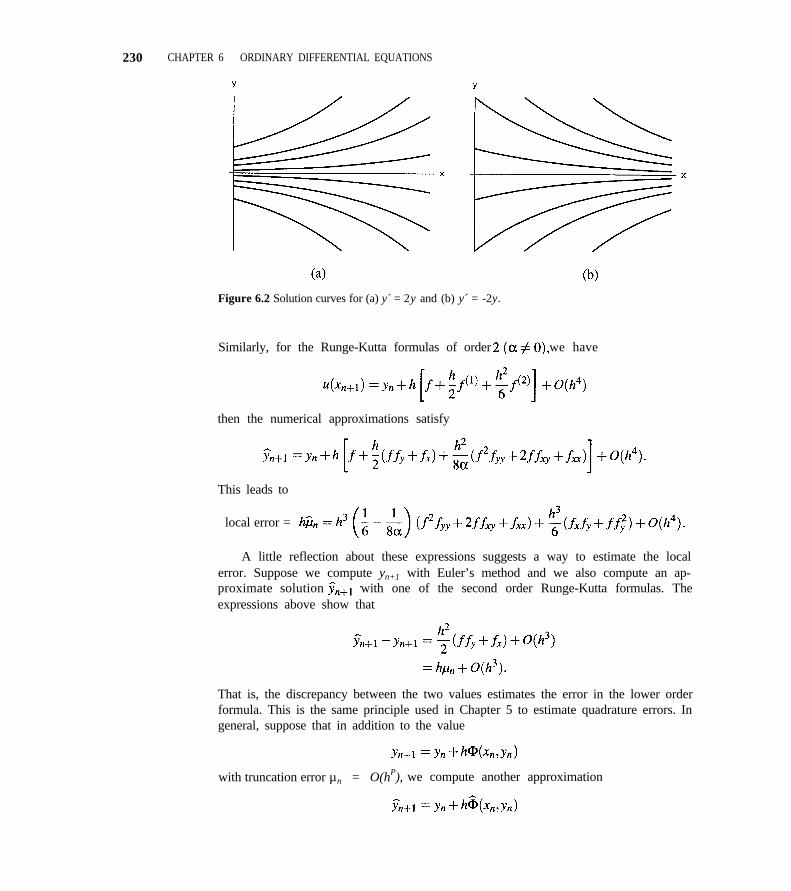
230 CHAPTER 6 ORDINARY DIFFERENTIAL EQUATIONS
Figure 6.2 Solution curves for (a) y´ = 2y and (b) y´ = -2y.
Similarly, for the Runge-Kutta formulas of order we have
then the numerical approximations satisfy
This leads to
local error =
A little reflection about these expressions suggests a way to estimate the localerror. Suppose we compute yn+1 with Euler’s method and we also compute an ap-proximate solution with one of the second order Runge-Kutta formulas. Theexpressions above show that
That is, the discrepancy between the two values estimates the error in the lower orderformula. This is the same principle used in Chapter 5 to estimate quadrature errors. Ingeneral, suppose that in addition to the value
with truncation error µn = O(hP), we compute another approximation
6.4 ERRORS-LOCAL AND GLOBAL 231
with truncation error of higher order, q > p. Then by definition
and, similarly,
which, on subtracting, shows that
Because goes to zero faster than we can estimate the local error by
local error
We would like to approximate the local solution u(xn+1). In view of the fact thatwe have a good estimate of the error in yn+l, why not try to improve it by takingout the error? This process, called local extrapolation, is here formally equivalent toadvancing the integration with the higher order approximation because
This tells us that local extrapolation will raise the effective order of the pair from p to q.Thus we can think of what is happening in two ways. One is that a formula of order p isbeing used with its result improved by local extrapolation. The other is that a formulaof order q is being used with the step size selected conservatively by pretending thatthe step is being taken with a formula of a lower order p. Because local extrapolationincreases the accuracy at no increase in cost, all the current production-grade codesbased on explicit Runge-Kutta methods use it.
A Runge-Kutta formula of order 4 requires (at least) four evaluations of F per stepand a companion formula of order 5 requires at least six. Just as with Gauss-Kronrodquadrature, the trick to being efficient is to derive the formulas as a pair in whichfunction evaluations are used in both formulas. R. England published such a pair offormulas in [5]. To advance from xn to xn + h, he takes a step of length h/ 2 with (6.2 1)to get the fourth order result and then another step of length h/2
to get the fourth order result By working with two half-steps, he hasenough function evaluations available that with only one extra evaluation, he is ableto form a fifth order approximation In this way, one extra functionevaluation is made every two half-steps to get an error estimate. An error estimate isused to control the local error and so give some credibility to the computed solution.It also allows the code to select the largest step size that will result in the error testbeing passed. Except in unusual cases, adaptation of the step size to the solution inthis way greatly increases the efficiency of integration. It corresponds to the adaptivequadrature schemes of Chapter 5.
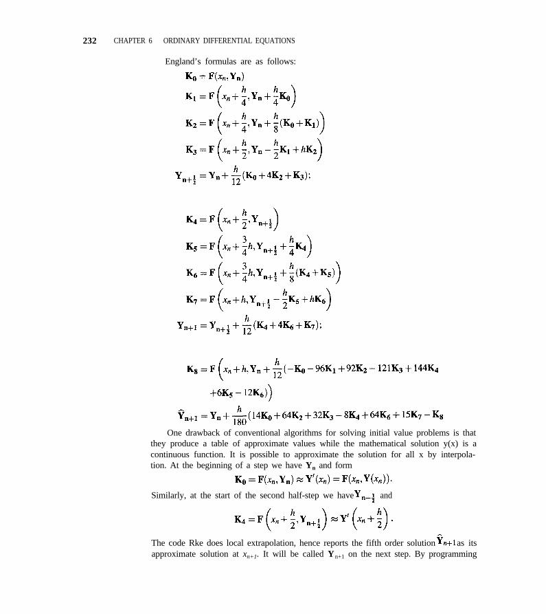
232 CHAPTER 6 ORDINARY DIFFERENTIAL EQUATIONS
England’s formulas are as follows:
One drawback of conventional algorithms for solving initial value problems is thatthey produce a table of approximate values while the mathematical solution y(x) is acontinuous function. It is possible to approximate the solution for all x by interpola-tion. At the beginning of a step we have Yn and form
Similarly, at the start of the second half-step we have and
The code Rke does local extrapolation, hence reports the fifth order solution as itsapproximate solution at xn+1. It will be called Yn+1 on the next step. By programming
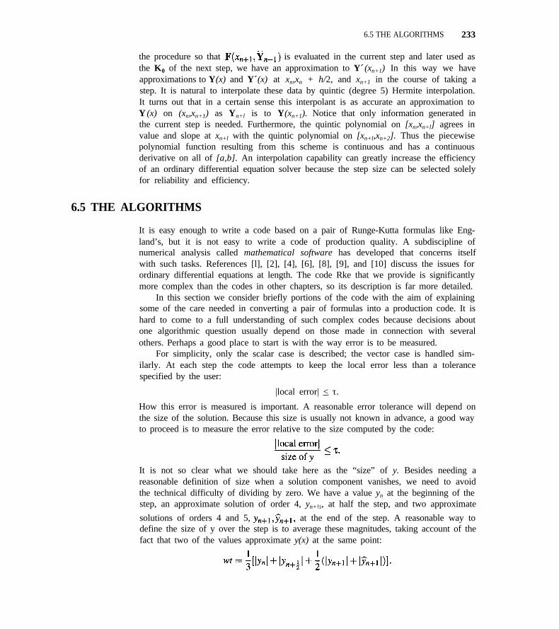
6.5 THE ALGORITHMS 233
the procedure so that is evaluated in the current step and later used asthe K0 of the next step, we have an approximation to Y´ (xn+1) In this way we haveapproximations to Y(x) and Y´(x) at xn,xn + h/2, and xn+1 in the course of taking astep. It is natural to interpolate these data by quintic (degree 5) Hermite interpolation.It turns out that in a certain sense this interpolant is as accurate an approximation toY (x) on (xn,xn+1) as Yn+l is to Y(xn+1). Notice that only information generated inthe current step is needed. Furthermore, the quintic polynomial on [xn,xn+l] agrees invalue and slope at xn+l with the quintic polynomial on [xn+l,xn+2]. Thus the piecewisepolynomial function resulting from this scheme is continuous and has a continuousderivative on all of [a,b]. An interpolation capability can greatly increase the efficiencyof an ordinary differential equation solver because the step size can be selected solelyfor reliability and efficiency.
6.5 THE ALGORITHMS
It is easy enough to write a code based on a pair of Runge-Kutta formulas like Eng-land’s, but it is not easy to write a code of production quality. A subdiscipline ofnumerical analysis called mathematical software has developed that concerns itselfwith such tasks. References [l], [2], [4], [6], [8], [9], and [10] discuss the issues forordinary differential equations at length. The code Rke that we provide is significantlymore complex than the codes in other chapters, so its description is far more detailed.
In this section we consider briefly portions of the code with the aim of explainingsome of the care needed in converting a pair of formulas into a production code. It ishard to come to a full understanding of such complex codes because decisions aboutone algorithmic question usually depend on those made in connection with severalothers. Perhaps a good place to start is with the way error is to be measured.
For simplicity, only the scalar case is described; the vector case is handled sim-ilarly. At each step the code attempts to keep the local error less than a tolerancespecified by the user:
|local error| < τ.
How this error is measured is important. A reasonable error tolerance will depend onthe size of the solution. Because this size is usually not known in advance, a good wayto proceed is to measure the error relative to the size computed by the code:
It is not so clear what we should take here as the “size” of y. Besides needing areasonable definition of size when a solution component vanishes, we need to avoidthe technical difficulty of dividing by zero. We have a value yn at the beginning of thestep, an approximate solution of order 4, yn+½, at half the step, and two approximate
solutions of orders 4 and 5, at the end of the step. A reasonable way todefine the size of y over the step is to average these magnitudes, taking account of thefact that two of the values approximate y(x) at the same point:
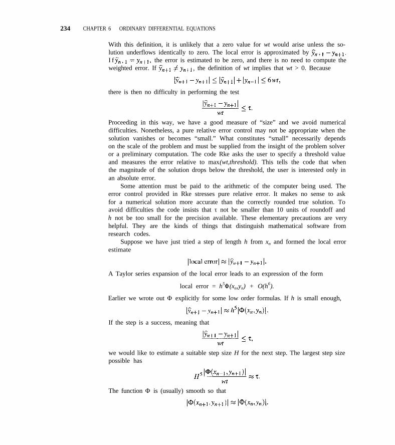
234 CHAPTER 6 ORDINARY DIFFERENTIAL EQUATIONS
With this definition, it is unlikely that a zero value for wt would arise unless the so-lution underflows identically to zero. The local error is approximated byI f the error is estimated to be zero, and there is no need to compute theweighted error. If the definition of wt implies that wt > 0. Because
there is then no difficulty in performing the test
Proceeding in this way, we have a good measure of “size” and we avoid numericaldifficulties. Nonetheless, a pure relative error control may not be appropriate when thesolution vanishes or becomes “small.” What constitutes “small” necessarily dependson the scale of the problem and must be supplied from the insight of the problem solveror a preliminary computation. The code Rke asks the user to specify a threshold valueand measures the error relative to max(wt,threshold). This tells the code that whenthe magnitude of the solution drops below the threshold, the user is interested only inan absolute error.
Some attention must be paid to the arithmetic of the computer being used. Theerror control provided in Rke stresses pure relative error. It makes no sense to askfor a numerical solution more accurate than the correctly rounded true solution. Toavoid difficulties the code insists that τ not be smaller than 10 units of roundoff andh not be too small for the precision available. These elementary precautions are veryhelpful. They are the kinds of things that distinguish mathematical software fromresearch codes.
Suppose we have just tried a step of length h from xn and formed the local errorestimate
A Taylor series expansion of the local error leads to an expression of the form
local error = h5ΦΦ (xn,yn) + O(h6).
Earlier we wrote out Φ explicitly for some low order formulas. If h is small enough,
If the step is a success, meaning that
we would like to estimate a suitable step size H for the next step. The largest step sizepossible has
The function Φ is (usually) smooth so that
6.5 THE ALGORITHMS 235
Writing H = αh we then find
so that the “optimal” H is
It is much too bold to try this H because if it is even slightly too large, the step willfail and this is expensive. Besides, after making all those approximations, we shouldnot take H too seriously. In practice a fraction of H is tried, or equivalently a fractionof τ is used in computing H, and an efficient fraction determined by experiment. InRke the tolerance aimed at is 0.6τ. This is equivalent to using about nine-tenths of the“optimal” H.
The same argument is used to obtain the step size for trying again after a failedstep. In either case we must program the process with some care. For example, wemust deal with the possibility that the estimated local error is zero. This technicaldifficulty highlights the fact that large increases or decreases cannot be justified by thearguments made. For this reason changes are limited to an order of magnitude. If alarge change is truly called for, this action allows a large change to be accumulatedover a few steps without the disastrous possibilities opened up by a large change in asingle step. In the case of a failed step we must be especially cautious about taking theestimated error at face value. In Rke we try the predicted value once, but if it fails, wesimply halve the step size until we get success.
For the numerical solution of ordinary differential equations there are two difficultranges of tolerances. It is to be expected that tolerances near limiting precision aredifficult, but it turns out that nominal tolerances are also difficult. Often users thinkthat because engineering accuracy of 10% will suffice in their use of the results, theycan keep their costs down by specifying such a large tolerance. This may result incheap results that are not reliable because the local error test may not keep the stepsize small enough to justify the approximations used throughout the code. Even if theresults are reliable, they can be far from what is desired because at crude tolerances thetrue, or global, errors can be much larger than the local errors controlled by the code.It is prudent to ask for accuracy of at least a couple of digits, so that the error controlof Rke emphasizes relative error and it is required that the relative tolerance τ < 0.01.
EXERCISES
6.15 Implement Euler’s method and a local error estimator and compare the estimated local error to the true localbased on Heun’s method. Apply it to the problem error. Also compare the global error at several points
to the general size of the local errors made in the com-y´ = 10(y-x), y(0) = 1/10 putations up to this point.
236 CHAPTER 6 ORDINARY DIFFERENTIAL EQUATIONS
6.6 THE CODE RKE
The routine Rke solves the initialdifferential equations of the form
value problem for a system of first order ordinary
A typical call for Rke in FORTRAN is
CALL RKE (F, NEQ, X, Y, H, FIRST, TOL, THRES, FLAG, STEP,YCOEFF, SCR, NDIM)
In C it is
Rke (f, neq, &x, y, &h, &first, tol, threshold, &flag, &step, ycoeff);
and it is
Rke (f, neq, x, y, h, first, tol, threshold, flag, step, ycoeff);
in C++.Input parameters to Rke are F, the name of the routine that defines the differential
equations [i.e., F(x, Y)]; NEQ, the number of first order differential equations to be in-tegrated; X, the initial value of the independent variable; Y, an array of dimension NEQcontaining the values of the solution components at X; H, step size for the current step(its sign determines the direction of integration); FIRST, a variable indicating whetherthis is the first or a subsequent step; a scalar TOL and a vector THRES (or thresholdin C and C++) are tolerances for the local error control; and NDIM > 6× NEQ, thedimension of the output vector YCOEFF and in FORTRAN of the auxiliary storagevector SCR. Output parameters are X, Y, the integration was advanced to X and Y isthe solution there; H, the step size suitable for the next step; FLAG, a flag reportingwhat the code did; STEP, the actual length of the step taken (output X minus inputX); and YCOEFF, an array of coefficient values for quintic Hermite interpolation to beused by the routine Yvalue.
Some of the variables in the call list require more explanation. The initial step sizeH informs the code of the scale of the problem. It should be small enough to capturechanges in the solution near the initial point. Also, the sign of H indicates the directionof integration because the code will try to step to X + H. After the first call, the codeprovides a suitable H for the next call.
The variable FIRST enables the code to initialize itself. The start of a new problemis indicated by input of FIRST = .TRUE. in FORTRAN and first = 1 in C or C++. Afterthe first call, the code sets FIRST = .FALSE. in FORTRAN and first = 0 in C and C++for subsequent calls. The error parameters TOL and THRES (or threshold in C andC++) tell the code how accurately the solution is to be computed. The vector THRESmust have dimension at least NEQ in the calling program. All components of THRESmust be nonnegative. The relative error tolerance TOL must satisfy
10u < TOL < 0.01
6.6 THE CODE RKE 237
where u is the unit roundoff of the machine. The tolerances are used by the codelocal error test at each step that requires roughly that
in a
|local error| < TOL max(|Y(I)|, THRES(I))
for component I of the vector Y. Setting THRES(I ) = 0 results in a pure relative errortest on the component. On the first call to the code, if some Y(I ) = 0, the correspondingTHRES(I) must be strictly positive. The size of the solution component is carefullydefined so that vanishing of the true solution at the current step is very unlikely tocause trouble. Any such trouble can be avoided by a positive value of THRES(I ) .
The code will not attempt to compute a solution at an accuracy unreasonable forthe computer being used. It will report if this situation arises. To continue the integra-tion after such a report, TOL and/or THRES must be increased. Note that Rke is anefficient code for moderate relative accuracies. For more than, say, six-digit accuracy,other methods are likely to be more efficient.
The true (global) error is the difference between the true solution of the initialvalue problem and the computed one. Nearly all initial value codes, including this one,control only the local error at each step, not the global error. Moreover, controllingthe local error in a relative sense does not necessarily result in the global error beingcontrolled in a relative sense. Roughly speaking, the codes produce a solution Y(x)that satisfies the differential equation with a residual R(x),
that is usually bounded in norm by the error tolerances. Usually the true accuracyof the computed Y is comparable to the error tolerances. This code will usually, butnot always, deliver a more accurate solution when the problem is solved again withsmaller tolerances. By comparing two such solutions a fairly reliable idea of the trueerror in the solution at the larger tolerances can be obtained.
The principal task of the code is to integrate one step from X toward X + H. Rou-tine Rke is organized so that subsequent calls to continue the integration involve little(if any) additional effort. The status of the integration is reported by the value of theFLAG parameter. After a successful step the routine Yvalue is used to approximatethe solution at points within the span of the step. A typical call is
CALL YVALUE(NEQ, X, STEP, YCOEFF, POINT, U)
in the FORTRAN version and
Yvalue(neq, x, step, ycoeff, point, u);
in the C and C++ versions. Input parameters are NEQ, X, STEP, YCOEFF (as returnedfrom Rke) and POINT, the point at which a solution is desired. The output is U(*), thevector of solution components at P. Routine Yvalue can be used only after a successfulstep by Rke and should be used only to interpolate the solution values on the interval[ X - STEP,X].
238 CHARTER 6 ORDINARY DIFFERENTIAL EQUATIONS
Example 6.8. To illustrate Rke, we solve the initial value problem
Y´1 = Y1, Y l(0) = 1Y´2 = -Y2, Y 2(0) = 1
on the interval [0,1] and print the solution at x = 1. The problem has the solutionYl(x) = ex, Y2(x) = e-x. As the solution component Y1 is increasing, a pure relativeerror test is appropriate and we set THRES(1) = 0. Y2, on the other hand, is decreasingand we choose THRES(2) = 10-5, which results in an absolute error test for small |Y2|.
XOUT = 1.00000000000000The numerical solution is 2.7182755628071 3.6787784616084E-01The true solution is 2.7182818284590 3.6787944117144E-01
Example 6.9. This example iThe initial value problem
llustrates the use of Yvalue in conjunction with Rke.
is integrated over the interval [0,10] and the solution tabulated at x = 0, 1, 2,. . . , 10.Note that Rke must be called before Yvalue. The output is as follows.
XOUT = 0.00XOUT = 1.00XOUT = 2.00XOUT = 3.00XOUT = 4.00XOUT = 5.00XOUT = 6.00XOUT = 7.00XOUT = 8.00XOUT = 9.00XOUT =10.00
Y(1) = 1.000000Y(1) = 1.298484Y(1) = 0.421178Y(1) =-1.634813Y(1) =-1.743960Y(1) =-0.878664
Y(1) = 1.187072Y(1) = 1.933030Y(1) = 1.245572Y(1) =-0.329599Y(1) =-2.008260
Y(2) = 1.000000
Y(2) =-0.367034Y(2) =-1.488951Y(2) =-1.485472Y(2) = 0.568922Y(2) = 1.258102
Y(2) = 2.521700Y(2) =-0.406833Y(2) =-0.963183Y(2) =-2.467240Y(2) =-0.034172
EXERCISES
Unless otherwise indicated, use 10-5 for tolerancevalues and 10-7 for the threshold values for the com-puting exercises.
in Exercise 6.4.
(a) y´ = -½y3, y(0) = 1; b = 3
(b) y´ = -2xy2, y(0) = 1; b = 16.16 Use Rke with a tolerance of 10-6 and threshold values
of 1 to calculate y(b) in the following cases. Check the(c) y´ = ¼y(1 - y/20), y(0) = 1; b = 5
computed output with the exact answers that are given (d) y´ = 100(sinx - y), y(0) = 0; b = 1
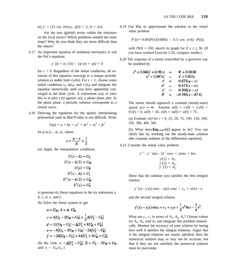
6.17
6.18
(e) y´ = (15 cos 10x)/y, y(0) = 2; b = π/4.
Are the true (global) errors within the toleranceon the local errors? Which problems needed the moststeps? Why do you think they are more difficult thanthe others?
An important equation of nonlinear mechanics is vander Pol’s equation:
x´´(t) + ε( x2(t) - 1)x´(t) + x(t) = 0
for ε > 0. Regardless of the initial conditions, all so-lutions of this equation converge to a unique periodicsolution (a stable limit cycle). For ε = 1, choose someinitial conditions t0, x(t0), and x´(t0) and integrate theequation numerically until you have apparently con-verged to the limit cycle. A convenient way to viewthis is to plot x´(t) against x(t), a phase plane plot. Inthe phase plane, a periodic solution corresponds to aclosed curve.
Deriving the equations for the quintic interpolatingpolynomial used in Rke/Yvalue is not difficult. Write
U(p) = a + bz + cz2 + dz3 + ez4 + fz5
for p in [x - ∆, x], where
(a) Apply the interpolation conditions
to generate six linear equations in the six unknowns a,b, c, d, e, and f.
(b) Solve the linear system to get
(In the code, α =
6.6 THE CODE RKE 239
6.19 Use Rke to approximate the solution to the initialvalue problem
P´(t) = 0.001P(t)[1000(1 - 0.3 cos πt/6) -P(t)],
with P(0) = 250; sketch its graph for 0 < t < 36. (Ifyou have worked Exercise 5.10, compare results.)
6.20 The response of a motor controlled by a governor canbe modeled by
The motor should approach a constant (steady-state)speed as Assume s(0) = s´(0) = u´(0) =θ (0) = 0, u(0) = 50, v(0) = w(0) = x(0) = 75.
(a) Evaluate v(t) for t = 0, 25, 50, 75, 100, 150, 200,250, 300, 400, 500.
(b) What does appear to be? You cancheck this by working out the steady-state solution(the constant solution of the differential equation).
6.21 Consider the initial value problem
y´´´ - y´´ sinx - 2y´ cosx + ysinx = lnx,
y(1) = A1,y´(1) = A2,y´´(1) = A3.
Show that the solution y(x) satisfies the first integralrelation
y´´(x) - y´(x) sinx - y(x) cosx = c2 + xl nx - x
and the second integral relation
What are c1, c2 in terms of A1, A2, A3? Choose valuesfor A1, A2, and A3 and integrate this problem numeri-cally. Monitor the accuracy of your solution by seeinghow well it satisfies the integral relations. Argue thatif the integral relations are nearly satisfied, then thenumerical solution may or may not be accurate, butthat if they are not satisfied, the numerical solution
and γ = UR-UL.) must be inaccurate.
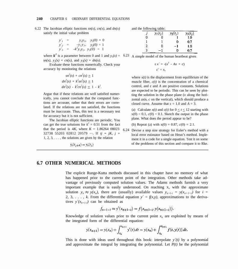
240 CHAPTER 6 ORDINARY DIFFERENTIAL EQUATIONS
6.22 The Jacobian elliptic functions sn(x), cn(x), and dn(x)satisfy the initial value problem
y´1 = y2y3, y1(0) = 0y´2 = -y 1 y3 , y2(0) = 1y´3 = -k2y1y2, y3(0) = 1
where k2 is a parameter between 0 and 1 and y1(x) = 6.23sn(x), y2(x) = cn(x), and y3(x) = dn(x).
Evaluate these functions numerically. Check youraccuracy by monitoring the relations
sn2(x) + cn2(x) = 1
dn2(x) + k2sn2(x) = 1
dn2(x) - k2cn2(x) = 1 - k2.
Argue that if these relations are well satisfied numer-ically, you cannot conclude that the computed func-tions are accurate, rather that their errors are corre-lated. If the relations are not satisfied, the functionsmust be inaccurate. Thus, this test is a necessary testfor accuracy but it is not sufficient.
The Jacobian elliptic functions are periodic. Youcan get the true solutions for k2 = 0.51 from the factthat the period is 4K, where K = 1.86264 08023 6.2432738 55203 02812 20579 ···. If tj = jK, j =1, 2, 3, . . . , the solutions are given by the relation
and the following table:
A simple model of the human heartbeat gives
ε x´ = -(x3 - Ax + c)
c´ = x,
where x(t) is the displacement from equilibrium of themuscle fiber, c(t) is the concentration of a chemicalcontrol, and ε and A are positive constants. Solutionsare expected to be periodic. This can be seen by plot-ting the solution in the phase plane (x along the hori-zontal axis, c on the vertical), which should produce aclosed curve. Assume that ε = 1.0 and A = 3.
(a) Calculate x(t) and c(t) for 0 < t < 12 starting withx(0) = 0.1, c(0) = 0.1. Sketch the output in the phaseplane. What does the period appear to be?
(b) Repeat (a) with x(0) = 0.87, c(0) = 2.1.
Devise a step size strategy for Euler’s method with alocal error estimator based on Heun’s method. Imple-ment it in a code for a single equation. Test it on someof the problems of this section and compare it to Rke.
6.7 OTHER NUMERICAL METHODS
The explicit Runge-Kutta methods discussed in this chapter have no memory of whathas happened prior to the current point of the integration. Other methods take ad-vantage of previously computed solution values. The Adams methods furnish a veryimportant example that is easily understood. On reaching X, with the approximatesolution yn y(xn), there are (usually) available values yn+l-i = y(xn+1+i) for i =2, 3, . . . , k. From the differential equation y´ = f(x,y), approximations to the deriva-tives y´(xn+1-i) can be obtained as
Knowledge of solution values prior to the current point xn are exploited by means ofthe integrated form of the differential equation:
This is done with ideas used throughout this book: interpolate y´(t) by a polynomialand approximate the integral by integrating the polynomial. Let P(t) be the polynomial
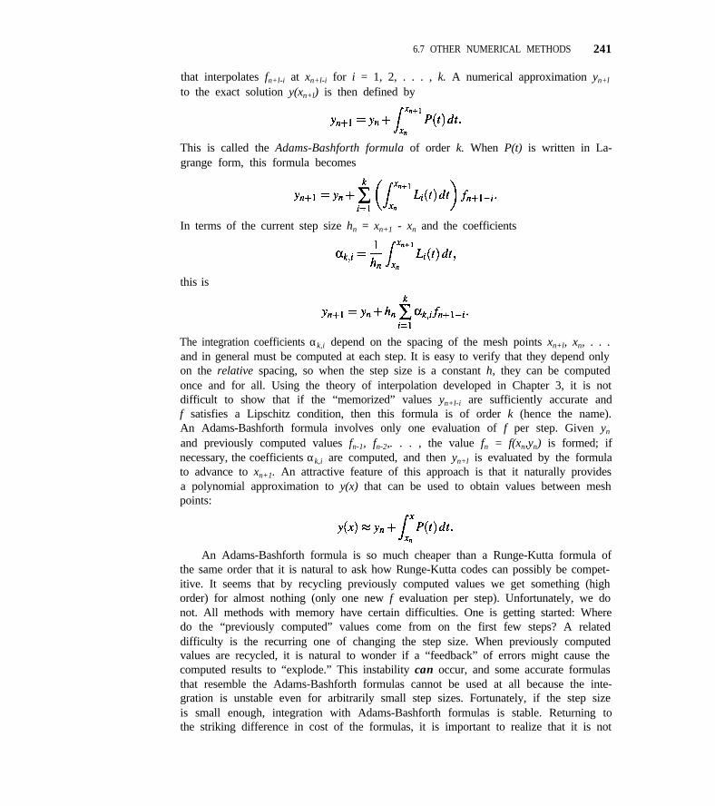
6.7 OTHER NUMERICAL METHODS 241
that interpolates fn+l-i at xn+l-i for i = 1, 2, . . . , k. A numerical approximation yn+l
to the exact solution y(xn+l) is then defined by
This is called the Adams-Bashforth formula of order k. When P(t) is written in La-grange form, this formula becomes
In terms of the current step size hn = xn+1 - xn and the coefficients
this is
The integration coefficients αk,i depend on the spacing of the mesh points xn+l, xn, . . .and in general must be computed at each step. It is easy to verify that they depend onlyon the relative spacing, so when the step size is a constant h, they can be computedonce and for all. Using the theory of interpolation developed in Chapter 3, it is notdifficult to show that if the “memorized” values yn+l-i are sufficiently accurate andf satisfies a Lipschitz condition, then this formula is of order k (hence the name).An Adams-Bashforth formula involves only one evaluation of f per step. Given yn
and previously computed values fn-1, fn-2,. . . , the value fn = f(xn,yn) is formed; ifnecessary, the coefficients αk,i are computed, and then yn+l is evaluated by the formulato advance to xn+1. An attractive feature of this approach is that it naturally providesa polynomial approximation to y(x) that can be used to obtain values between meshpoints:
An Adams-Bashforth formula is so much cheaper than a Runge-Kutta formula ofthe same order that it is natural to ask how Runge-Kutta codes can possibly be compet-itive. It seems that by recycling previously computed values we get something (highorder) for almost nothing (only one new f evaluation per step). Unfortunately, we donot. All methods with memory have certain difficulties. One is getting started: Wheredo the “previously computed” values come from on the first few steps? A relateddifficulty is the recurring one of changing the step size. When previously computedvalues are recycled, it is natural to wonder if a “feedback” of errors might cause thecomputed results to “explode.” This instability can occur, and some accurate formulasthat resemble the Adams-Bashforth formulas cannot be used at all because the inte-gration is unstable even for arbitrarily small step sizes. Fortunately, if the step sizeis small enough, integration with Adams-Bashforth formulas is stable. Returning tothe striking difference in cost of the formulas, it is important to realize that it is not
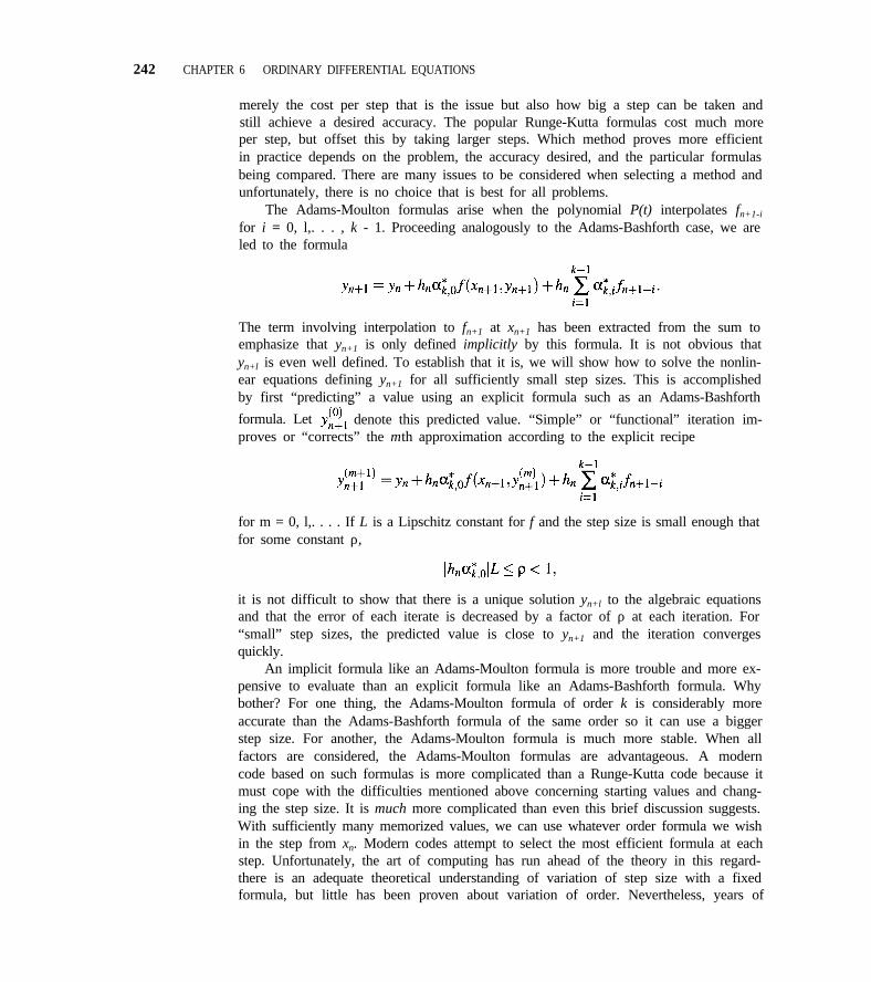
242 CHAPTER 6 ORDINARY DIFFERENTIAL EQUATIONS
merely the cost per step that is the issue but also how big a step can be taken andstill achieve a desired accuracy. The popular Runge-Kutta formulas cost much moreper step, but offset this by taking larger steps. Which method proves more efficientin practice depends on the problem, the accuracy desired, and the particular formulasbeing compared. There are many issues to be considered when selecting a method andunfortunately, there is no choice that is best for all problems.
The Adams-Moulton formulas arise when the polynomial P(t) interpolates fn+1-i
for i = 0, l,. . . , k - 1. Proceeding analogously to the Adams-Bashforth case, we areled to the formula
The term involving interpolation to fn+1 at xn+1 has been extracted from the sum toemphasize that yn+1 is only defined implicitly by this formula. It is not obvious thatyn+l is even well defined. To establish that it is, we will show how to solve the nonlin-ear equations defining yn+1 for all sufficiently small step sizes. This is accomplishedby first “predicting” a value using an explicit formula such as an Adams-Bashforth
formula. Let denote this predicted value. “Simple” or “functional” iteration im-proves or “corrects” the mth approximation according to the explicit recipe
for m = 0, l,. . . . If L is a Lipschitz constant for f and the step size is small enough thatfor some constant ρ,
it is not difficult to show that there is a unique solution yn+l to the algebraic equationsand that the error of each iterate is decreased by a factor of ρ at each iteration. For“small” step sizes, the predicted value is close to yn+1 and the iteration convergesquickly.
An implicit formula like an Adams-Moulton formula is more trouble and more ex-pensive to evaluate than an explicit formula like an Adams-Bashforth formula. Whybother? For one thing, the Adams-Moulton formula of order k is considerably moreaccurate than the Adams-Bashforth formula of the same order so it can use a biggerstep size. For another, the Adams-Moulton formula is much more stable. When allfactors are considered, the Adams-Moulton formulas are advantageous. A moderncode based on such formulas is more complicated than a Runge-Kutta code because itmust cope with the difficulties mentioned above concerning starting values and chang-ing the step size. It is much more complicated than even this brief discussion suggests.With sufficiently many memorized values, we can use whatever order formula we wishin the step from xn. Modern codes attempt to select the most efficient formula at eachstep. Unfortunately, the art of computing has run ahead of the theory in this regard-there is an adequate theoretical understanding of variation of step size with a fixedformula, but little has been proven about variation of order. Nevertheless, years of
6.7 OTHER NUMERICAL METHODS 243
heavy usage of codes that vary the order have demonstrated that they do “work” andthat the variation of the order is very important to the efficiency of such codes.
Another natural approach to approximating the solutions of differential equationsis based on numerical differentiation. Again using a basic idea of this book, we startby interpolating previously computed solution values yn, yn+1, . . . ,yn+l-k as well asthe new one yn+l by a polynomial P(t). The derivative of the solution at xn+1 is thenapproximated by P´(xn+1). This approximation is tied to the differential equation atxn+1 by requiring that
A formula for yn+l is obtained by writing P(t) in Lagrange form and using it in theP´(xn+1) term of the equation. For certain practical reasons it is usual with this familyof formulas to work with a constant step size h. Making this assumption, carrying outthe substitution, and scaling by h lead to a formula of the form
This is a member of a family known as backward differentiation formulas, or justBDFs. They were popularized by Gear [6] and are sometimes known as Gear’s formu-las. Obviously, these formulas are implicit like the Adams-Moulton formulas. Theyare not nearly as accurate as the Adams-Moulton formulas of the same order, andformulas of orders 7 and up cannot be used because they are not stable (hence notconvergent) as the step size tends to zero. The reason they are interesting is that at theorders for which they are stable, they are much more stable than explicit Runge-Kuttaand Adams formulas. Before discussing their usage, some general remarks about thestep size are necessary.
The selection of the step size is affected by a number of issues. The one thatreceives the most attention is choosing the step size sufficiently small to obtain thedesired accuracy. We have also seen that for some methods the step size might haveto be reduced to produce an answer at a desired point. There are other less obviousconstraints on the step size. Earlier we touched on the matter that the step size mighthave to be restricted so as to evaluate an implicit formula efficiently and also alludedto the issue of restricting the step size in order to make the integration stable. Thereare problems of great practical interest called stiff for which these other restrictionswill cause an explicit Runge-Kutta method or an Adams-Moulton formula evaluatedby simple iteration to need a step size very much smaller than that permitted by the ac-curacy of the formula. The excellent stability properties of the BDFs have made themthe most popular formulas for solving such problems. They cannot be evaluated bysimple iteration because it restricts the step size too much. In practice, a modificationof the Newton iteration described in Chapter 4 is used to solve the nonlinear algebraicequations for yn+1. This has many disagreeable consequences due to the necessity ofapproximating partial derivatives and solving systems of linear equations. Each step isvery expensive compared to a Runge-Kutta or Adams method, but when the problemis stiff, the steps can be so much larger that this is a bargain. Indeed, the solutionof a problem that is quite stiff is impractical with codes not specifically intended forsuch problems. As with the Adams formulas, modern codes based on the BDFs vary
244 CHAPTER 6 ORDINARY DIFFERENTIAL EQUATIONS
the order as well as the step size. Stiff problems are difficult technically as well aspractically and how to solve them is an active area of research.
There is a large literature on the solution of the initial value problem for a sys-tem of ordinary differential equations. References [4], [8], and [9] provide usefulorientation, especially in regard to the software available. State-of-the-art codes areavailable from netlib: RKSUITE [l] makes available explicit Runge-Kutta formulasof three different orders. ODE/STEP/INTRP [10] is a variable step, variable orderAdams-Bashforth-Moulton code. The methods of RKSUITE and ODE/STEP/INTRPare not appropriate for stiff problems. Both suites of codes diagnose stiffness when itis responsible for unsatisfactory performance. VODE [2] is a variable step, variableorder code that makes available two kinds of methods, Adams-Moulton formulas anda variant of the BDFs. The computing environments MATLAB and MATHCAD providecodes based on a variety of methods, including some not mentioned here, but the codethat is to be tried first (assuming that the problem is not stiff) is an explicit Runge-Kutta code. Mathematics provides a single code that, like VODE, makes availableboth Adams-Moulton methods and the BDFs. It is unusual in that the code attemptsto recognize stiffness and select an appropriate method automatically.
6.8 CASE STUDY 6
The restricted three-body problem is obtained from Newton’s equations of motionfor the gravitational attraction of three bodies when one has a mass infinitesimal incomparison to the other two. For example, the position (x,y) of a spaceship or satellitemoving under the influence of the earth and the moon in a coordinate system rotatingso as to keep the positions of the earth and moon fixed changes according to
Here
and µ = 1/82.45, µ* = 1 - µ. More insight is possible when the general equationsof motion are reduced to those of the restricted three-body problem, but it is still notpossible to determine orbits analytically. A search using high precision computationidentified several periodic orbits. One has initial conditions x(0) = 1.2, x´(0) = 0,y(0) = 0, and y´(0) = -1.04935750983031990726. The period of this orbit is aboutT = 6.19216933131963970674. Integration of this problem with Rke is straightfor-ward after the equations are written as a first order system by introducing the vectorof unknowns y(t) = (x(t),y(t),x´(t),y´(t))T. The orbit displayed in Figure 6.3 wascomputed using 10-6 for TOL and all components of THRESHOLD. Although the
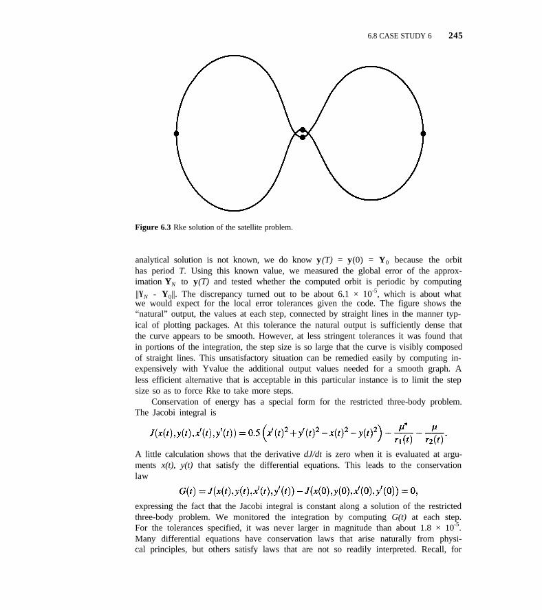
6.8 CASE STUDY 6 245
Figure 6.3 Rke solution of the satellite problem.
analytical solution is not known, we do know y(T) = y(0) = Y0 because the orbithas period T. Using this known value, we measured the global error of the approx-imation YN to y(T) and tested whether the computed orbit is periodic by computing||YN - Y0||. The discrepancy turned out to be about 6.1 × 10⁻⁵, which is about whatwe would expect for the local error tolerances given the code. The figure shows the“natural” output, the values at each step, connected by straight lines in the manner typ-ical of plotting packages. At this tolerance the natural output is sufficiently dense thatthe curve appears to be smooth. However, at less stringent tolerances it was found thatin portions of the integration, the step size is so large that the curve is visibly composedof straight lines. This unsatisfactory situation can be remedied easily by computing in-expensively with Yvalue the additional output values needed for a smooth graph. Aless efficient alternative that is acceptable in this particular instance is to limit the stepsize so as to force Rke to take more steps.
Conservation of energy has a special form for the restricted three-body problem.The Jacobi integral is
A little calculation shows that the derivative dJ/dt is zero when it is evaluated at argu-ments x(t), y(t) that satisfy the differential equations. This leads to the conservationlaw
expressing the fact that the Jacobi integral is constant along a solution of the restrictedthree-body problem. We monitored the integration by computing G(t) at each step.For the tolerances specified, it was never larger in magnitude than about 1.8 × 10⁻⁵.Many differential equations have conservation laws that arise naturally from physi-cal principles, but others satisfy laws that are not so readily interpreted. Recall, for
246 CHAPTER 6 ORDINARY DIFFERENTIAL EQUATIONS
example, the conservation law we used in Case Study 4 to solve the Lotka-Volterraequations in the phase plane. Conservation laws are consequences of the form of thedifferential equations. It does not follow that numerical approximations will satisfythe laws, and generally speaking they do not. However, they must satisfy the lawsapproximately. To see this, suppose that G(t) = G(t,y (t)) = 0 for any solution y(t) ofa differential equation y´ = F(t , y ). If yn y(tn), then linearization tells us that
Evidently the residual of the numerical solution in the conservation law is of the sameorder as the global error of the numerical solution, y(tn) - yn. This observation helpsus understand the size of the residual we found in integrating the periodic earth-moonorbit. It is worth remarking that solutions of a system of differential equations mightsatisfy several conservation laws.
The conservation laws mentioned so far are nonlinear, but others arising fromconservation of mass, charge balance, and the like are linear. A linear conservationlaw for the equation y´ = F( t , y) arises mathematically when there is a constant vectorv such that vT F( t ,u) = 0 for all arguments (t ,u). If y(t) is a solution of the equation,then
implying that G(t) = vT y (t) - vT y (0) = 0. A simple example is provided by a systemof equations that describes a certain radioactive decay chain:
The right-hand sides here sum to zero, hence the system satisfies a linear conservationlaw with vT = (1, 1,. . . , l)T. Figure 6.4 shows the solution of this system with initialcondition y(0) = (1, 0,. . . ,0) computed using Rke with TOL equal to 10-3 and allT
components of THRESHOLD equal to 10-10. Despite the modest relative accuracyrequested, the error in the conservation law was at the roundoff level, specifically amaximum of 4.4 × 10-l6 in the MATLAB environment on the workstation we used.This illustrates an interesting fact: all standard numerical methods produce approxi-mations that satisfy linear conservation laws exactly. This is easy to show for explicitRunge-Kutta formulas. In advancing from xn to xn + h, such a formula has the form
Each stage Ki has the form F( x*,Y*) for arguments (x*,Y*) that are defined in termsof xn, h, and the previous stages. The details do not matter, for all we need here is thatv T K i = 0 because vT F( t ,u) = 0 for all arguments (t ,u). It then follows immediately
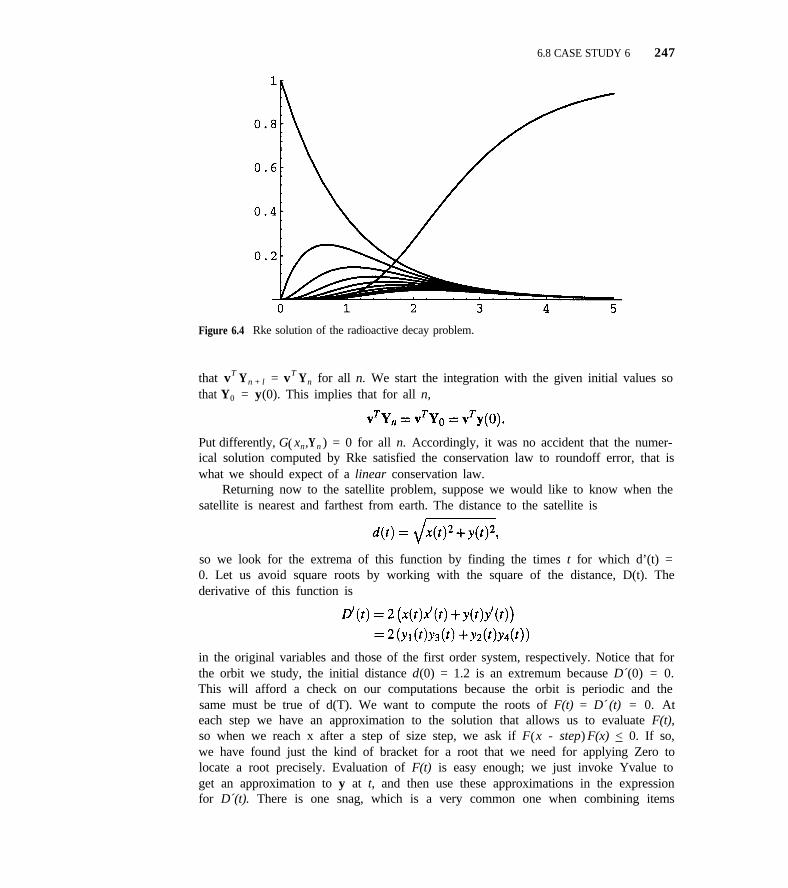
6.8 CASE STUDY 6 247
Figure 6.4 Rke solution of the radioactive decay problem.
that vT Yn + l = vT Yn for all n. We start the integration with the given initial values sothat Y0 = y(0). This implies that for all n,
Put differently, G( xn,Yn ) = 0 for all n. Accordingly, it was no accident that the numer-ical solution computed by Rke satisfied the conservation law to roundoff error, that iswhat we should expect of a linear conservation law.
Returning now to the satellite problem, suppose we would like to know when thesatellite is nearest and farthest from earth. The distance to the satellite is
so we look for the extrema of this function by finding the times t for which d’(t) =0. Let us avoid square roots by working with the square of the distance, D(t). Thederivative of this function is
in the original variables and those of the first order system, respectively. Notice that forthe orbit we study, the initial distance d(0) = 1.2 is an extremum because D´(0) = 0.This will afford a check on our computations because the orbit is periodic and thesame must be true of d(T). We want to compute the roots of F(t) = D´ (t) = 0. Ateach step we have an approximation to the solution that allows us to evaluate F(t),so when we reach x after a step of size step, we ask if F(x - step) F(x) < 0. If so,we have found just the kind of bracket for a root that we need for applying Zero tolocate a root precisely. Evaluation of F(t) is easy enough; we just invoke Yvalue toget an approximation to y at t, and then use these approximations in the expressionfor D´(t). There is one snag, which is a very common one when combining items
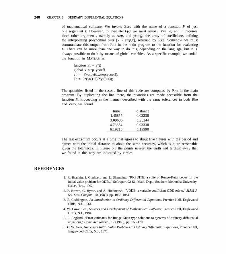
248 CHAPTER 6 ORDINARY DIFFERENTIAL EQUATIONS
of mathematical software. We invoke Zero with the name of a function F of justone argument t. However, to evaluate F(t) we must invoke Yvalue, and it requiresthree other arguments, namely x, step, and ycoeff, the array of coefficients definingthe interpolating polynomial over [x - step,x], returned by Rke. Somehow we mustcommunicate this output from Rke in the main program to the function for evaluatingF. There can be more than one way to do this, depending on the language, but it isalways possible to do it by means of global variables. As a specific example, we codedthe function in MATLAB as
function Ft = F(t)global x step ycoeffyt = Yvalue(t,x,step,ycoeff);Ft = 2*(yt(1:2)´*yt(3:4));
The quantities listed in the second line of this code are computed by Rke in the mainprogram. By duplicating the line there, the quantities are made accessible from thefunction F. Proceeding in the manner described with the same tolerances in both Rkeand Zero, we found
time distance1.45857 0.033383.09606 1.262444.73354 0.033386.19210 1.19998
The last extremum occurs at a time that agrees to about five figures with the period andagrees with the initial distance to about the same accuracy, which is quite reasonablegiven the tolerances. In Figure 6.3 the points nearest the earth and farthest away thatwe found in this way are indicated by circles.
REFERENCES
1. R. Brankin, I. Gladwell, and L. Shampine, “RKSUITE: a suite of Runge-Kutta codes for theinitial value problem for ODES,” Softreport 92-S1, Math. Dept., Southern Methodist University,Dallas, Tex., 1992.
2. P. Brown, G. Byrne, and A. Hindmarsh, “VODE: a variable-coefficient ODE solver,” SIAM J.Sci. Stat. Comput., 10 (1989), pp. 1038-1051.
3. E. Coddington, An Introduction to Ordinary Differential Equations, Prentice Hall, EnglewoodCliffs, N.J., 1961.
4. W. Cowell, ed., Sources and Development of Mathematical Software, Prentice Hall, EnglewoodCliffs, N.J., 1984.
5. R. England, “Error estimates for Runge-Kutta type solutions to systems of ordinary differentialequations,” Computer Journal, 12 (1969), pp. 166-170.
6. C. W. Gear, Numerical Initial Value Problems in Ordinary Differential Equations, Prentice Hall,Englewood Cliffs, N.J., 1971.
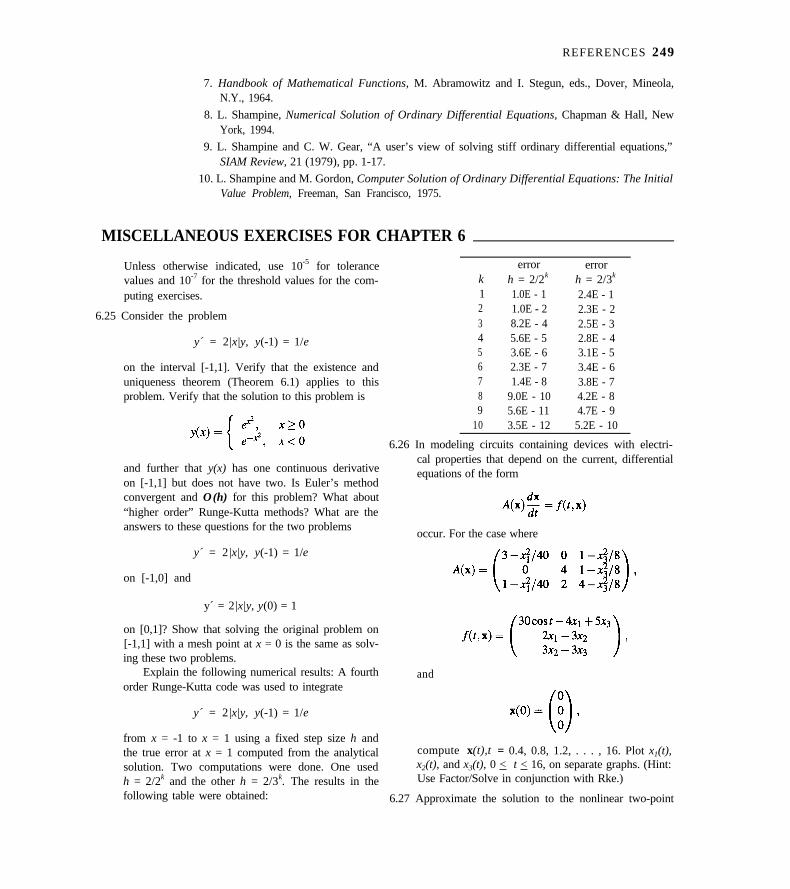
REFERENCES 249
7. Handbook of Mathematical Functions, M. Abramowitz and I. Stegun, eds., Dover, Mineola,N.Y., 1964.
8. L. Shampine, Numerical Solution of Ordinary Differential Equations, Chapman & Hall, NewYork, 1994.
9. L. Shampine and C. W. Gear, “A user’s view of solving stiff ordinary differential equations,”SIAM Review, 21 (1979), pp. 1-17.
10. L. Shampine and M. Gordon, Computer Solution of Ordinary Differential Equations: The InitialValue Problem, Freeman, San Francisco, 1975.
MISCELLANEOUS EXERCISES FOR CHAPTER 6
Unless otherwise indicated, use 10-5 for tolerancevalues and 10-7 for the threshold values for the com-puting exercises.
6.25 Consider the problem
y´ = 2|x|y, y(-1) = 1/e
on the interval [-1,1]. Verify that the existence anduniqueness theorem (Theorem 6.1) applies to thisproblem. Verify that the solution to this problem is
and further that y(x) has one continuous derivativeon [-1,1] but does not have two. Is Euler’s methodconvergent and O(h) for this problem? What about“higher order” Runge-Kutta methods? What are theanswers to these questions for the two problems
y´ = 2|x|y, y(-1) = 1/e
on [-1,0] and
y´ = 2|x|y, y(0) = 1
on [0,1]? Show that solving the original problem on[-1,1] with a mesh point at x = 0 is the same as solv-ing these two problems.
Explain the following numerical results: A fourthorder Runge-Kutta code was used to integrate
y´ = 2|x|y, y(-1) = 1/e
from x = -1 to x = 1 using a fixed step size h andthe true error at x = 1 computed from the analyticalsolution. Two computations were done. One usedh = 2/2k and the other h = 2/3k. The results in thefollowing table were obtained:
k123456789
10
error errorh = 2/2k h = 2/3k
1.0E - 1 2.4E - 11.0E - 2 2.3E - 28.2E - 4 2.5E - 35.6E - 5 2.8E - 43.6E - 6 3.1E - 52.3E - 7 3.4E - 61.4E - 8 3.8E - 7
9.0E - 10 4.2E - 85.6E - 11 4.7E - 93.5E - 12 5.2E - 10
6.26 In modeling circuits containing devices with electri-cal properties that depend on the current, differentialequations of the form
occur. For the case where
and
compute x(t),t = 0.4, 0.8, 1.2, . . . , 16. Plot x1(t),x2(t), and x3(t), 0 < t < 16, on separate graphs. (Hint:Use Factor/Solve in conjunction with Rke.)
6.27 Approximate the solution to the nonlinear two-point
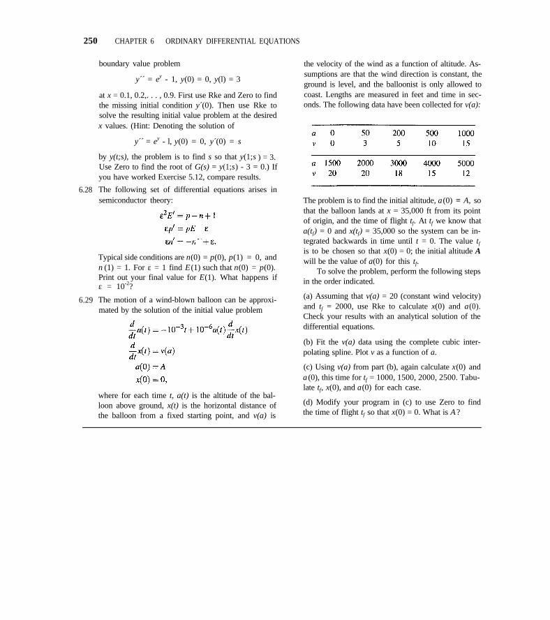
250 CHAPTER 6 ORDINARY DIFFERENTIAL EQUATIONS
6.28
6.29
boundary value problem
y´´ = ey - 1, y(0) = 0, y(l) = 3
at x = 0.1, 0.2,. . . , 0.9. First use Rke and Zero to findthe missing initial condition y´(0). Then use Rke tosolve the resulting initial value problem at the desiredx values. (Hint: Denoting the solution of
y´´ = ey - l, y(0) = 0, y´(0) = s
by y(t;s), the problem is to find s so that y(1;s ) = 3.Use Zero to find the root of G(s) = y(1;s) - 3 = 0.) Ifyou have worked Exercise 5.12, compare results.
The following set of differential equations arises insemiconductor theory:
Typical side conditions are n(0) = p(0), p(1) = 0, andn (1) = 1. For ε = 1 find E(1) such that n(0) = p(0).Print out your final value for E(1). What happens ifε = 10-2?
The motion of a wind-blown balloon can be approxi-mated by the solution of the initial value problem
where for each time t, a(t) is the altitude of the bal-loon above ground, x(t) is the horizontal distance ofthe balloon from a fixed starting point, and v(a) is
the velocity of the wind as a function of altitude. As-sumptions are that the wind direction is constant, theground is level, and the balloonist is only allowed tocoast. Lengths are measured in feet and time in sec-onds. The following data have been collected for v(a):
The problem is to find the initial altitude, a(0) = A, sothat the balloon lands at x = 35,000 ft from its pointof origin, and the time of flight tf. At tf we know thata(tf) = 0 and x(tf) = 35,000 so the system can be in-tegrated backwards in time until t = 0. The value tf
is to be chosen so that x(0) = 0; the initial altitude Awill be the value of a(0) for this tf.
To solve the problem, perform the following stepsin the order indicated.
(a) Assuming that v(a) = 20 (constant wind velocity)and tf = 2000, use Rke to calculate x(0) and a(0).Check your results with an analytical solution of thedifferential equations.
(b) Fit the v(a) data using the complete cubic inter-polating spline. Plot v as a function of a.
(c) Using v(a) from part (b), again calculate x(0) anda (0), this time for tf = 1000, 1500, 2000, 2500. Tabu-late tf, x(0), and a(0) for each case.
(d) Modify your program in (c) to use Zero to findthe time of flight tf so that x(0) = 0. What is A?
APPENDIX A
NOTATION AND SOME THEOREMSFROM THE CALCULUS
We assume that the reader is familiar with the topics normally covered in the under-graduate analytical geometry and calculus sequence. For purpose of reference, wepresent some standard notation used in this book and a few theorems from the calcu-lus.
A.1 NOTATION
[a,b ], the interval consisting of the real numbers x such that a < x < b.
(a,b), the interval consisting of the real numbers x such that a < x < b.
lies in the interval [a, b].
belongs to the class of functions having a first derivative continuous onthe interval [a,b].
belongs to the class of functions having an nth derivative continuous on
[a,b]The norm ||f|| of a function f(x) continuous on the interval [a,b] is the maximumvalue of |f(x)| over the interval.
and so on, denote
partial differentiation.
0.d1 d2 . . . dn(e) stands for 0.d1 d2 . . . dn × 10e; for example, 0.123(4) means 0.123 ×10⁴. More often, we use 0.123E4 for this.
251
252 APPENDIX A NOTATION AND SOME THEOREMS FROM THE CALCULUS
is approximately equal to.
f(x+) = limit of f(x + η) as with η > 0, the limit from the right.
f(x-) = limit of f( x - η ) as with η > 0, the limit from the left.
<<, much less.
v = (v1v2··· vn), notation for a vector.
The norm ||v|| of a vector v is the maximum magnitude component of the vector.
q(h) = 0(hk) as means that there are (unknown) constants h0, K such that|q(h)| < Khk for all 0 < h < h0.
A.2 THEOREMS
Theorem. Intermediate Value Theorem. Let f(x) be a continuous function onthe interval [a,b]. If for some number a and for some x1 ,x2 [a, b] we have f(xl) <α < f(x2), then there is a point c [a,b] such that a = f(c).
Theorem. Rolle’s Theorem. Let f(x) be continuous on the finite interval [a,b]and differentiable on (a, b). If f(a) = f(b) = 0, there is a point c (a,b) such thatf´(c) = 0.
Theorem. Mean Value Theorem for Integrals. Let g(x) be a nonnegative func-tion integrable on the interval [a,b]. If f(x) is continuous on [a,b], then there is a pointc [a,b] such that
Theorem. Mean Value Theorem for Derivatives. Let f(x) be continuous onthe finite interval [a,b] and differentiable on (a,b). Then there is a point c (a,b)such that
Theorem. Taylor’s Theorem (for f(x)). Let f(x) have n + 1 continuous deriva-tives on (a,b) for some n > 0 and let x,x0 (a, b). Then
f(x) = Pn(x) + Rn+1(x),
where
and
A.2 THEOREMS 253
for some z between x0 and x.
Theorem. Taylor’s Theorem (for f(x,y)). Let (x0,y0) and (x0 + ξy0 + η) begiven points and assume that f(x,y) is n + 1 times continuously differentiable in someneighborhood of the line L(x0, y0;x0 + ξ,y0 + η) connecting (x0,y0) and (x0 + ξ,y0 +η). Then
for some 0 < θ < 1. [The point (x0 + θξ,y0 + θη) is an unknown point on the line L.]For n = 2, the formula without remainder becomes
Theorem. Let f(x) be a continuous function on the finite interval [a,b]. Thenf(x) assumes its maximum and minimum values on [a, b]; that is, there are pointsx1 ,x2 [a,b] such that
f(x1) < f(x) < f(x2)
for all x [a,b].
Theorem. Integration by Parts. Let f(x) and g(x) e real-valued functionsbwith derivatives continuous on [a,b]. Then
Theorem. Fundamental Theorem of the Integral Calculus. Let f(x) be con-tinuous on the interval [a,b], and let
Then F(x) is differentiable on (a, b) and
F´(x) = f(x).
Theorem. Common Maclaurin Series. For any real number x,
254 APPENDIX A NOTATION AND SOME THEOREMS FROM THE CALCULUS
For |x| < 1,
For discussions and proofs of these theorems, see A. Taylor, Advanced Calculus, Wiley,New York, 1983.
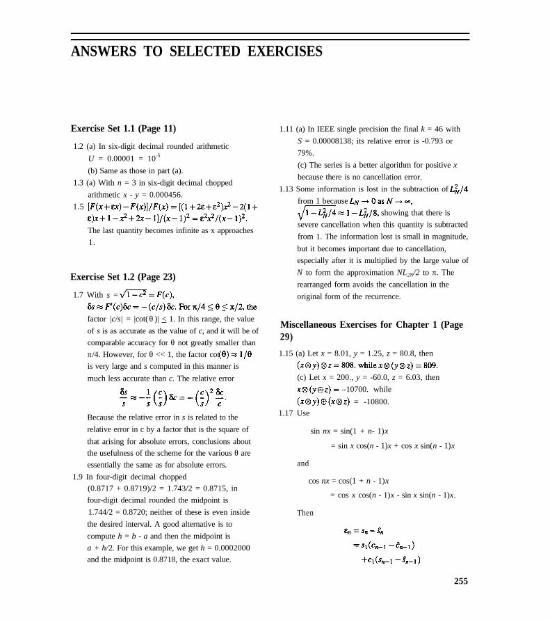
ANSWERS TO SELECTED EXERCISES
Exercise Set 1.1 (Page 11)
1.2 (a) In six-digit decimal rounded arithmetic
U = 0.00001 = 10-5
(b) Same as those in part (a).
1.3 (a) With n = 3 in six-digit decimal chopped
arithmetic x - y = 0.000456.
1.5
The last quantity becomes infinite as x approaches
1.
Exercise Set 1.2 (Page 23)
1.7 With s =
factor |c/s| = |cot( θ )| < 1. In this range, the value
of s is as accurate as the value of c, and it will be of
comparable accuracy for θ not greatly smaller than
π/4. However, for θ << 1, the factor cot
is very large and s computed in this manner is
much less accurate than c. The relative error
Because the relative error in s is related to the
relative error in c by a factor that is the square of
that arising for absolute errors, conclusions about
the usefulness of the scheme for the various θ are
essentially the same as for absolute errors.
1.9 In four-digit decimal chopped
(0.8717 + 0.8719)/2 = 1.743/2 = 0.8715, in
four-digit decimal rounded the midpoint is
1.744/2 = 0.8720; neither of these is even inside
the desired interval. A good alternative is to
compute h = b - a and then the midpoint is
a + h/2. For this example, we get h = 0.0002000
and the midpoint is 0.8718, the exact value.
1.11 (a) In IEEE single precision the final k = 46 with
S = 0.00008138; its relative error is -0.793 or
79%.
(c) The series is a better algorithm for positive x
because there is no cancellation error.
1.13 Some information is lost in the subtraction of
from 1 because
showing that there is
severe cancellation when this quantity is subtracted
from 1. The information lost is small in magnitude,
but it becomes important due to cancellation,
especially after it is multiplied by the large value of
N to form the approximation NL2N/2 to π. The
rearranged form avoids the cancellation in the
original form of the recurrence.
Miscellaneous Exercises for Chapter 1 (Page29)
1.15 (a) Let x = 8.01, y = 1.25, z = 80.8, then
(c) Let x = 200., y = -60.0, z = 6.03, then
-10700. while
= -10800.1.17 Use
sin nx = sin(1 + n- 1)x
= sin x cos(n - 1)x + cos x sin(n - 1)x
and
cos nx = cos(1 + n - 1)x
= cos x cos(n - 1)x - sin x sin(n - 1)x.
Then
255
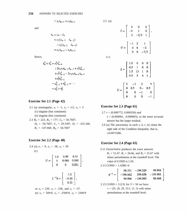
256 ANSWERS TO SELECTED EXERCISES
2.5 (a)
and
Hence, ( c )
Exercise Set 2.1 (Page 42)
2.1 (a) nonsingular; x1 = -1, x2 = 1/2, x3 = 3
(c) singular (but consistent)
(e) singular (but consistent)
2.3 RE = 223, RA = 177, Ch = 56.7607,
Dh = -56.7607, Cv = 29.3397, Dv = -252.340,
Bv = -147.660, Bh, = 56.7607
Exercise Set 2.2 (Page 48)
2.4 (a) x1 = 9, x2 = -36, x3 = 30
(c)
so x3 = 220, x2 = -230, and x1 = -37.
(e) x1 = 500/9, x2 = -2500/9, x3 = 2300/9
Exercise Set 2.3 (Page 61)
2.7 r = (0.000772, 0.000350) and
s = (0.000001, -0.000003), so the more accurate
answer has the larger residual.
2.9 (a) The uncertainty in each xi is ± ||x| times the
right side of the Condition Inequality, that is,
±0.0075386.
Exercise Set 2.4 (Page 63)
2.11 Factor/Solve produces the exact answers
R1 = 51.67, R2 = 26.66, and R3 = 31.67 with
minor perturbations at the roundoff level. The
value of COND is 1.50.
2.13 COND = 1.438E+4
2.15 COND = 112.9; for V = 50 we have
v = (35, 26, 20, 15.5, 11, 5) with minor
perturbations at the roundoff level.
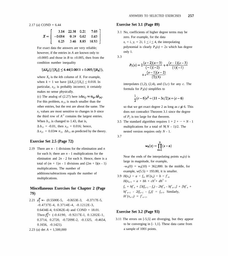
2.17 (a) COND = 6.44
For exact data the answers are very reliable;
however, if the entries in A are known only to
±0.0005 and those in B to ±0.005, then from the
condition number inequality
where Xk is the kth column of X. For example,
when k = 1 we have ||∆Xk||/||Xk|| < 0.018. In
particular, x21 is probably incorrect; it certainly
makes no sense physically.
(c) The analog of (2.27) here is
For this problem, α23 is much smaller than the
other entries, but the rest are about the same. The
x3 values are most sensitive to changes in b since
the third row of A-1 contains the largest entries.
When b11 is changed to 1.43, that is,
∆ b11 = -0.01, then x21 = 0.016; hence,
∆ x21 = 0.03 α21 ∆b11 as predicted by the theory.
Exercise Set 2.5 (Page 72)
2.19 There are n - 1 divisions for the elimination and n
for each b; there are n - 1 multiplications for the
elimination and 2n - 2 for each b. Hence, there is a
total of (m + 1)n - 1 divisions and (2m + l)(n - 1)
multiplications. The number of
additions/subtractions equals the number of
multiplications.
Miscellaneous Exercises for Chapter 2 (Page79)
2.21 (0.5500E-5, -0.l653E-3, -0.3717E-5,
-0.4737E-4, 0.3714E-4, -0.1212E-3,
0.6434E-4, 0.6362E-4) and COND = 18.01.
Then = (-0.6190, -0.9217E-l, 0.1202E-1,
0.3714, 0.2720, -0.7209E-2, -0.1325, -0.4654,
0.1656, -0.1421).
2.23 (a) det A = 1,500,000
ANSWERS TO SELECTED EXERCISES 257
Exercise Set 3.1 (Page 89)
3.1
3.3
3.5
3.7
3.9
No, coefficients of higher degree terms may be
zero. For example, for the data
xi = i, yi = 2i, 1 < i < 4, the interpolating
polynomial is clearly P4(x) = 2x which has degree
only 1.
interpolates (1,2), (2,4), and (3,c) for any c. The
formula for P3(x) simplifies to
so that we get exact degree 2 as long as c 6. This
does not contradict Theorem 3.1 since the degree
of P2 is too large for that theorem.
The standard algorithm requires 1 + 2 + ··· + N - 1
multiplications for a total of N( N - 1)/2. The
nested version requires only N - 1.
Near the ends of the interpolating points w9(x) is
large in magnitude, for example,
-w9(0) = w9(10) = 362,880. In the middle, for
example, w(5.5) = 193.80, it is smaller.
H(xn) = a = fn, H´(xn) = b = f´n,
H(xn+l = a + bh + ch2+ dh3 =
fn + hf´n + [3(fn+1 - fn) - 2hf´n - hf´n+1] + [hf´n +
hf´n+1 - 2(fn+1 - fn)] = fn+l. Similarly,H´(xn+l) = f´n+1.
Exercise Set 3.2 (Page 93)
3.11 The errors on [-5,5] are diverging, but they appear
to be converging in [- 1,1]. These data came from
a sample of 1001 points.
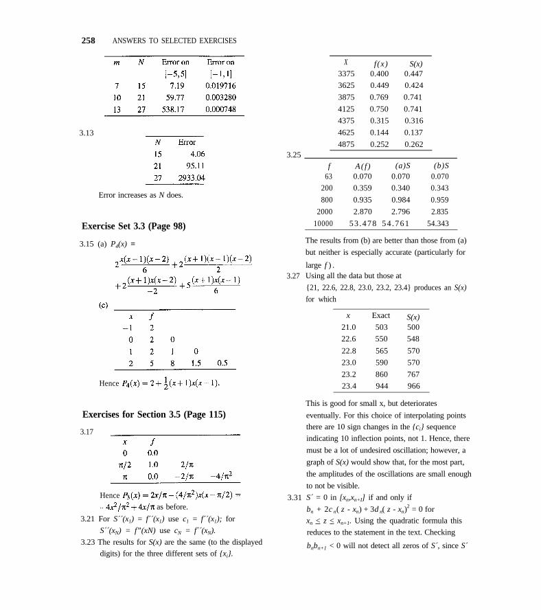
258 ANSWERS TO SELECTED EXERCISES
3.13
Error increases as N does.
Exercise Set 3.3 (Page 98)
3.15 (a) P4(x) =
Hence
Exercises for Section 3.5 (Page 115)
3.17
Hence
as before.
3.21 For S´´(x1) = f´´(x1) use c1 = f´´(x1); for
S´´(xN) = f”(xN) use cN = f´´(xN).
3.23 The results for S(x) are the same (to the displayed
digits) for the three different sets of {xi}.
3.25
3.27
3.31
X f(x) S(x)3375 0.400 0.447
3625 0.449 0.424
3875 0.769 0.741
4125 0.750 0.741
4375 0.315 0.316
4625 0.144 0.137
4875 0.252 0.262
f A( f ) (a)S (b)S63 0.070 0.070 0.070
200 0.359 0.340 0.343
800 0.935 0.984 0.959
2000 2.870 2.796 2.835
10000 53 .478 54 .761 54.343
The results from (b) are better than those from (a)
but neither is especially accurate (particularly for
large f ) .Using all the data but those at
{21, 22.6, 22.8, 23.0, 23.2, 23.4} produces an S(x)
for which
x Exact S(x)21.0 503 500
22.6 550 548
22.8 565 570
23.0 590 570
23.2 860 767
23.4 944 966
This is good for small x, but deteriorates
eventually. For this choice of interpolating points
there are 10 sign changes in the {ci} sequence
indicating 10 inflection points, not 1. Hence, there
must be a lot of undesired oscillation; however, a
graph of S(x) would show that, for the most part,
the amplitudes of the oscillations are small enough
to not be visible.
S´ = 0 in [xn,xn+I] if and only if
bn + 2c n( z - xn) + 3d n( z - xn)2 = 0 for
xn < z < xn+1. Using the quadratic formula this
reduces to the statement in the text. Checking
bnbn+1 < 0 will not detect all zeros of S´, since S´
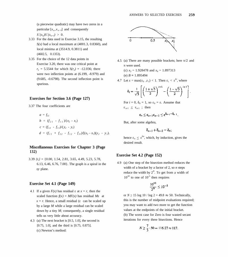
ANSWERS TO SELECTED EXERCISES 259
3.33
3.35
(a piecewise quadratic) may have two zeros in a
particular [xn ,x n +l] and consequently
S´(xn)S´(xn+l) > 0.For the data used in Exercise 3.15, the resulting
S(x) had a local maximum at (4001.3, 0.8360), and
local minima at (3514.9, 0.3811) and
(4602.5, 0.1353).
For the choice of the 12 data points in
Exercise 3.20, there was one critical point at
re = 5.5544 for which S(re) = -12.036; there
were two inflection points at (6.199, -8.979) and
(9.685, -0.6798). The second inflection point is
spurious.
Exercises for Section 3.6 (Page 127)
3.37 The four coefficients are
a = f11
b = (f 2 1 - f 1 1 )/(x2 - x1)
c = (f12 - f11)/( y2 - y1)
d = (f 1 1 + f 2 2 - f 1 2 - f 2 l)/[(x2 - x1)(y2 - y1).
Miscellaneous Exercises for Chapter 3 (Page132)
3.39 {ti} = {0.00, 1.54, 2.81, 3.65, 4.49, 5.23, 5.78,
6.13, 6.46, 6.76, 7.00}. The graph is a spiral in the
xy plane.
Exercise Set 4.1 (Page 149)
4.1
4.3
If a given F(x) has residual ε at x = r, then the
scaled function f(x) = MF(x) has residual Mε at
x = r. Hence, a small residual (ε) can be scaled up
by a large M while a large residual can be scaled
down by a tiny M; consequently, a single residual
tells us very little about accuracy.
(a) The next bracket is [0.5, 1.0], the second is
[0.75, 1.0], and the third is [0.75, 0.875].
(c) Newton’s method:
4.5
4.7
(a) There are many possible brackets; here π/2 and
π were used.
(c) x3 = 1.928478 and x4 = 1.897313
(e) B = 1.895494
Let ε = max(ε0 ,ε1) < 1. Then εi < εδi, where
For i = 0, δ0 = 1, so ε0 = ε. Assume that
ε n-1 < εn-1 ; then
But, after some algebra,
hence εn < εδn, which, by induction, gives the
desired result.
Exercise Set 4.2 (Page 152)
4.9 (a) One step of the bisection method reduces the
width of a bracket by a factor of 2, so n steps
reduce the width by 2N. To get from a width of
1010 to one of 10-5 then requires
or N > 15 log 10 / log 2 = 49.8 50. Technically,
this is the number of midpoint evaluations required;
you may want to add two more to get the function
values at the endpoints of the initial bracket.
(b) The worst case for Zero is four wasted secant
iterations for every three bisections. Hence
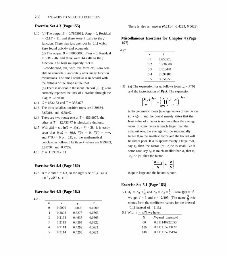
260 ANSWERS TO SELECTED EXERCISES
Exercise Set 4.3 (Page 155) There is also an answer (0.2114, -0.4293, 0.0623).
4.10
4.11
4.13
4.15
4.17
4.19
(a) The output B = 0.7853982, Flag = 0, Residual
= -2.1E - 11, and there were 7 calls to the f
function. There was just one root in [0,1] which
Zero found quickly and accurately.
(d) The output B = 0.8000003, Flag = 0, Residual
= 5.3E - 46, and there were 44 calls to the f
function. The high multiplicity root is
ill-conditioned, yet, with this form off, Zero was
able to compute it accurately after many function
evaluations. The small residual is in accord with
the flatness of the graph at the root.
(h) There is no root in the input interval [0, 1]; Zero
correctly reported the lack of a bracket through the
Flag = -2 value.
C = 633.162 and T = 353.878
The three smallest positive roots are 1.30654,
3.67319, and 6.58462.
There are two roots: one at T = 456.9975, the
other at T = 12,733.77 is physically dubious.
With f(k) = ω0 ln(1 + k)/(1 - k) - 2k, it is easily
seen that f(-k) = -f(k), f(0) = 0, f(1-) =and f´´(k) > 0 on [0,l), so the mathematical
conclusions follow. The three k values are 0.99933,
0.95750, and 0.77552.
E = 1.1903E- 11
Exercise Set 4.4 (Page 160)
4.23 m = 2 and α = 1/3, so the right side of (4.14) is
10 - 6 10-7.
Exercise Set 4.5 (Page 162)
4.25n x y z
0 0.5000 1.OOOO 0.0000
1 0.2808 0.6278 0.0365
2 0.2138 0.4635 0.0565
3 0.2113 0.4305 0.0622
4 0.2114 0.4293 0.0623
5 0.2114 0.4293 0.0623
Miscellaneous Exercises for Chapter 4 (Page167)
4.27x t
0.1 0.656578
0.2 1.236000
0.3 1.918448
0.4 2.694180
0.5 3.556555
4.31 (a) The expression for a0 follows from a0 = P(0)
and the factorization of P(x). The expression
is the geometric mean (average value) of the factors
(σ - ri)/ri, and the bound merely states that the
least value of a factor is no more than the average
value. If some factor is much larger than the
smallest one, the average will be substantially
larger than the smallest factor and the bound will
be rather poor. If σ is approximately a large root,
say rj, then the factor (σ - rj)/ rj is small. But if
some root, say rk, is much smaller than σ, that is,
|rk| >> |σ|, then the factor
is quite large and the bound is poor.
Exercise Set 5.1 (Page 183)
5.1 A1 = A4 = and A2 = A3 = From f(x) = x4
we get d = 3 and c = -2/405. (The name -rule
comes from the coefficient values for the interval
[0,1] instead of [-1,1].)
5.3 With h = π/N we have
N N-panel trapezoid
60 0.811148922853
100 0.811155733422
140 0.811155735194
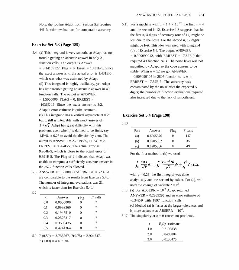
Note: the routine Adapt from Section 5.3 requires
441 function evaluations for comparable accuracy.
Exercise Set 5.3 (Page 189)
5.4
5.5
5.7
5.9
(a) This integrand is very smooth, so Adapt has no
trouble getting an accurate answer in only 21
function calls. The output is Answer
= 3.14159122, Flag = 0, Errest = 1.431E-5. Since
the exact answer is π, the actual error is 1.431E-5,
which was what was estimated by Adapt.
(d) This integrand is highly oscillatory, yet Adapt
has little trouble getting an accurate answer in 49
function calls. The output is ANSWER
= 1.5000000, FLAG = 0, ERREST =
-1036E-16. Since the exact answer is 3/2,
Adapt’s error estimate is quite accurate.
(f) This integrand has a vertical asymptote at 0.25
but it still is integrable with exact answer of
1 + Adapt has great difficulty with this
problem, even when f is defined to be finite, say
1.E+8, at 0.25 to avoid the division by zero. The
output is ANSWER = 2.7319539, FLAG = 2,
ERREST = 9.264E-5. The actual error is
9.264E-5, which is close to the actual error of
9.691E-5. The Flag of 2 indicates that Adapt was
unable to compute a sufficiently accurate answer in
the 3577 function calls allowed.
ANSWER = 1.500000 and ERREST = -2.4E-18
are comparable to the results from Exercise 5.4d.
The number of integrand evaluations was 21,
which is faster than for Exercise 5.4d.
x Answer Flag F calls
0.0 0.0000000 0 7
0.1 0.0993360 0 7
0.2 0.1947510 0 7
0.3 0.2826317 0 7
0.4 0.3599435 0 7
0.5 0.4244364 0 7
T (0.50) = 3.736767, T(0.75) = 3.904747,
T (1.00) = 4.187184.
ANSWERS TO SELECTED EXERCISES 261
5.11 For a machine with u = 1.4 × 10⁻¹⁷, the first n = 4
and the second is 12. Exercise 1.3 suggests that for
the first n, 4 digits of accuracy (out of 17) might be
lost due to the noise. For the second n, 12 digits
might be lost. This idea was used with integrand
(b) of Exercise 5.4. The output ANSWER
= 0.909090912, with ERREST = -7.82E-9 that
required 49 function calls. The noise level was not
magnified by Adapt, so the code appears to be
stable. When n = 12 we got ANSWER
= 0.909099105 in 2807 function calls with
ERREST = -7.82E-6. The accuracy was
contaminated by the noise after the expected 5
digits; the number of function evaluations required
also increased due to the lack of smoothness.
Exercise Set 5.4 (Page 198)
5.13
5.15
5.17
Part Answer Flag F calls
(a) 0.6205370 0 147
(b) 0.6205362 0 35
(c) 0.6205366 0 49
For the first method in (b) we used
with ε = 0.23; the first integral was done
analytically and the second by Adapt. For (c), we
used the change of variable t = x2.
(a) For ABSERR = 10-9 Adapt returned
ANSWER = 0.2865295 and an error estimate of
-0.34E-9 with 1897 function calls.
(c) Method (a) is faster at the larger tolerances and
is more accurate at ABSERR = 10-9.
The singularity at x = 0 causes no problems.
t E1(t) estimate
1.0 0.2193838
2.0 0.0489004
3.0 0.0130475
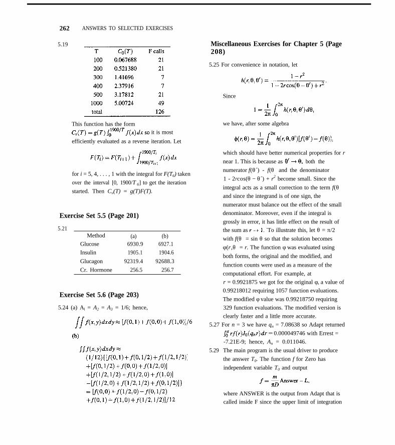
262 ANSWERS TO SELECTED EXERCISES
5.19
This function has the formit is most
efficiently evaluated as a reverse iteration. Let
for i = 5, 4, . . . , 1 with the integral for F(T6) taken
over the interval [0, 1900/T 6] to get the iteration
started. Then Cv(T) = g(T)F(T).
Exercise Set 5.5 (Page 201)
5.21Method (a) (b)
Glucose 6930.9 6927.1
Insulin 1905.1 1904.6
Glucagon 92319.4 92688.3
Cr. Hormone 256.5 256.7
Exercise Set 5.6 (Page 203)
5.24 (a) Al = A2 = A3 = 1/6; hence,
Miscellaneous Exercises for Chapter 5 (Page208)
5.25 For convenience in notation, let
Since
we have, after some algebra
which should have better numerical properties for r
near 1. This is because as both the
numerator f(θ´) - f(θ) and the denominator
1 - 2rcos(θ − θ´) + r2 become small. Since the
integral acts as a small correction to the term f(θ)and since the integrand is of one sign, the
numerator must balance out the effect of the small
denominator. Moreover, even if the integral is
grossly in error, it has little effect on the result of
the sum as To illustrate this, let θ = π/2
with f(θ) = sin θ so that the solution becomes
φ(r,θ) = r. The function φ was evaluated using
both forms, the original and the modified, and
function counts were used as a measure of the
computational effort. For example, at
r = 0.9921875 we got for the original φ, a value of
0.99218012 requiring 1057 function evaluations.
The modified φ value was 0.99218750 requiring
329 function evaluations. The modified version is
clearly faster and a little more accurate.
5.27 For n = 3 we have qn = 7.08638 so Adapt returned
0.000049746 with Errest =
-7.21E-9; hence, An = 0.011046.
5.29 The main program is the usual driver to produce
the answer T0. The function f for Zero has
independent variable T0 and output
where ANSWER is the output from Adapt that is
called inside F since the upper limit of integration
is T0. The result is T0 = 246.73.
Exercise Set 6.1 (Page 216)
6.1
6.3
6.5
6.7
Clearly y(0) = 0 and y´(x) = 0 for 0 < x < c and
y´ = (x - c)/2 for c < x < b. The limits as
are the same in both cases, so y´ is continuous on
[0, b]. Also, for 0 < x < c,
and for c < x < b,
so that y(x) satisfies the differential equation.
Recall that Dawson’s integral is the expression
Now, y(0) = 0 and differentiation shows that
Obviously, y´ is continuous on [0,b] for any finite b.
(a) fy = 2y; the partial derivative is not bounded for
all y and so does not satisfy a Lipschitz condition
for 0 < x < π/2.
(c) fy = 1/x; since |fy| < 1/1 = 1 for x in [1,2], the
function f does satisfy a Lipschitz condition with
constant L = 1.
(e) fy = cos x cos y; since |fy| < 1.1 for any x and
y, the function f does satisfy a Lipschitz condition
with constant L = 1.
(a) One solution is Y1 = u, Y2 = u´, Y3 = u´´, and
Y4 = u´´´ ; then Y´1 = Y2, Y´2 = Y3, Y´3 = Y4, and
Y´4 = cos αt + tY1 - etY2.
(c) One solution is Y1 = u, Y2 = u´, and Y3 = v; then
solving the system for u´´ and v´, we have
Hence Y´1 = Y2, Y´2 = 2t + (3 cos t)/4 - 7Y1/4 - Y3,
and Y´3 = 2t - (cos t)/4 - 3Y1/4.
ANSWERS TO SELECTED EXERCISES 263
(e) One solution is Yl = u, Y2 = u´, Y3 = u´´,
Y4 = u(3), Y5 = u(4), and Y6 = u(5) ; then Y´1 = Y2,
Y´2 = Y3, Y´3 = Y4, Y´4 = Y5, Y´5 = Y6, and
Y´6 = et - Y1Y2.
Exercise Set 6.2 (Page 221)
6.9 For h = l/40 the error at 0.5 is 0.0021; at 1.0 the
error is 0.0010. For h = l/80 the error at 0.5 is
0.0023; at 1.0 the error is 0.00116. For both x
values the error does drop by a factor of 2 as h is
halved. To achieve an absolute error of 10-6 in
magnitude would require h 0.000011.
Exercise Set 6.3 (Page 227)
6.11
6.13
For h = l/40 the error at 0.5 is -0.l434E-4; at
1.0 the error is -0.l395E-4. For h = l/80 the
error at 0.5 is -0.3564E-5; at 1.0 the error is
-0.3471. For both x values the error does drop by
a factor of 4 as h is halved. To achieve an absolute
error of 10-6 in magnitude would require
h 0.0067.
To show that y(r) can be computed via the formula
y(r) = Pry + Qr we use induction. The result is true
for r = 2 since
y´´ = P´1y + P1y´ + Q´1
= P´1y + P1(P1y + Q1) + Q´1
= (P´1 + P1 · P1)y + (Q´1 + Q1P1)
= P2y + Q2.
Assume it to be true for r = k; then
y(k+1) = P´ky + Pky´ + Q´k
= P´ky + Pk(P1y + Ql) + Q´k
= (P´k + P1Pk)y + (Q´k + Q1Pk)
=P k + l y + Q k + l .
A fifth order formula is obtained by dropping the
remainder term in the expression
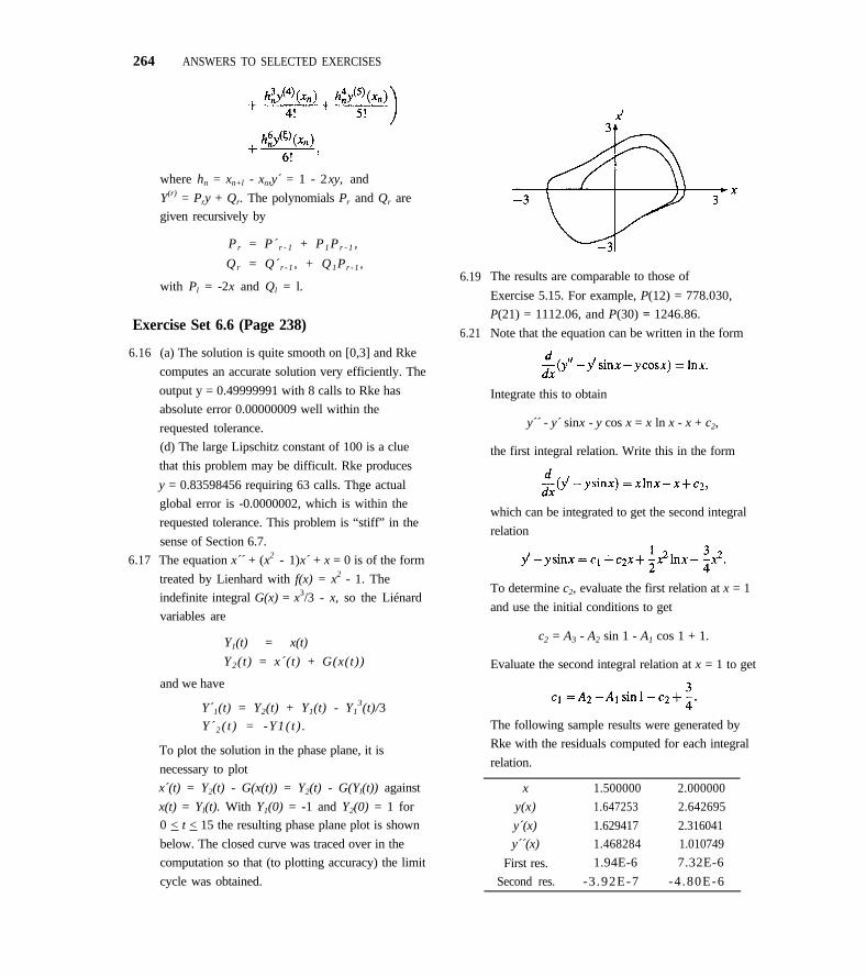
264 ANSWERS TO SELECTED EXERCISES
where hn = xn+l - xn,y´ = 1 - 2xy, and
Y(r) = Pry + Qr. The polynomials Pr and Qr are
given recursively by
P r = P´ r - 1 + P1 P r - 1 ,
Q r = Q´r - 1 , + Q1Pr - 1 ,
with Pl = -2x and Ql = l.
Exercise Set 6.6 (Page 238)
6.16
6.17
6.21
(a) The solution is quite smooth on [0,3] and Rke
computes an accurate solution very efficiently. The
output y = 0.49999991 with 8 calls to Rke has
absolute error 0.00000009 well within the
requested tolerance.
(d) The large Lipschitz constant of 100 is a clue
that this problem may be difficult. Rke produces
y = 0.83598456 requiring 63 calls. Thge actual
global error is -0.0000002, which is within the
requested tolerance. This problem is “stiff” in the
sense of Section 6.7.
The equation x´´ + (x2 - 1)x´ + x = 0 is of the form
treated by Lienhard with f(x) = x2 - 1. The
indefinite integral G(x) = x3/3 - x, so the Liénard
variables are
The results are comparable to those of
Exercise 5.15. For example, P(12) = 778.030,
P(21) = 1112.06, and P(30) = 1246.86.
Note that the equation can be written in the form
Integrate this to obtain
y´´ - y´ sinx - y cos x = x ln x - x + c2,
the first integral relation. Write this in the form
which can be integrated to get the second integral
relation
Y1(t) = x(t)
Y2(t) = x´(t) + G(x(t))
and we have
To determine c2, evaluate the first relation at x = 1
and use the initial conditions to get
c2 = A3 - A2 sin 1 - A1 cos 1 + 1.
Evaluate the second integral relation at x = 1 to get
Y´1(t) = Y2(t) + Y1(t) - Y13(t)/3
Y´2 ( t ) = -Y1( t ) .
To plot the solution in the phase plane, it is
necessary to plot
The following sample results were generated by
Rke with the residuals computed for each integral
relation.
x´(t) = Y2(t) - G(x(t)) = Y2(t) - G(Yl(t)) against x
x(t) = Yl(t). With Y1(0) = -1 and Y2(0) = 1 for y(x)
0 < t < 15 the resulting phase plane plot is shown y´(x)
below. The closed curve was traced over in the y´´(x)
computation so that (to plotting accuracy) the limit First res.
cycle was obtained. Second res.
6.19
1.500000 2.000000
1.647253 2.642695
1.629417 2.316041
1.468284 1.010749
1.94E-6 7.32E-6
-3 .92E-7 -4 .80E-6
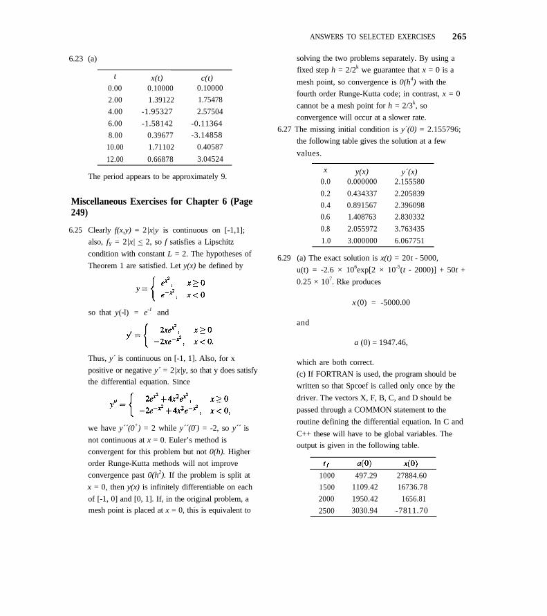
ANSWERS TO SELECTED EXERCISES 265
6.23 (a)
t x(t) c(t)0.00 0.10000 0.10000
2.00 1.39122 1.75478
4.00 -1.95327 2.57504
6.00 -1.58142 -0.11364
8.00 0.39677 -3.14858
10.00 1.71102 0.40587
12.00 0.66878 3.04524
The period appears to be approximately 9.
Miscellaneous Exercises for Chapter 6 (Page249)
6.25 Clearly f(x,y) = 2|x|y is continuous on [-1,1];
also, fY = 2|x| < 2, so f satisfies a Lipschitz
condition with constant L = 2. The hypotheses of
Theorem 1 are satisfied. Let y(x) be defined by
so that y(-l) = e-1 and
Thus, y´ is continuous on [-1, 1]. Also, for x
positive or negative y´ = 2|x|y, so that y does satisfy
the differential equation. Since
we have y´´(0+) = 2 while y´´(0-) = -2, so y´´ is
not continuous at x = 0. Euler’s method is
convergent for this problem but not 0(h). Higher
order Runge-Kutta methods will not improve
convergence past 0(h2). If the problem is split at
x = 0, then y(x) is infinitely differentiable on each
of [-1, 0] and [0, 1]. If, in the original problem, amesh point is placed at x = 0, this is equivalent to
solving the two problems separately. By using a
fixed step h = 2/2k we guarantee that x = 0 is a
mesh point, so convergence is 0(h4) with the
fourth order Runge-Kutta code; in contrast, x = 0
cannot be a mesh point for h = 2/3k, so
convergence will occur at a slower rate.
6.27 The missing initial condition is y´(0) = 2.155796;
the following table gives the solution at a few
values.
x y(x) y´(x)0.0 0.000000 2.155580
0.2 0.434337 2.205839
0.4 0.891567 2.396098
0.6 1.408763 2.830332
0.8 2.055972 3.763435
1.0 3.000000 6.067751
6.29 (a) The exact solution is x(t) = 20t - 5000,
u(t) = -2.6 × 10⁶exp[2 × 10⁻⁵(t - 2000)] + 50t +
0.25 × 10⁷. Rke produces
x (0) = -5000.00
and
a (0) = 1947.46,
which are both correct.
(c) If FORTRAN is used, the program should be
written so that Spcoef is called only once by the
driver. The vectors X, F, B, C, and D should be
passed through a COMMON statement to the
routine defining the differential equation. In C and
C++ these will have to be global variables. The
output is given in the following table.
1000 497.29 27884.60
1500 1109.42 16736.78
2000 1950.42 1656.81
2500 3030.94 -7811.70

INDEX
Absolute error, 1
Accuracy
of linear system algorithms, 48-61
of polynomial interpolation, 98-101
of quadrature, 184-187
of spline interpolation, 111-113
Adams-Bashforth formula, 241
Adams-Moulton formula, 242
Adams methods, 240-243
Adapt (code), 188-189
Adaptive quadrature, 184-188
AVINT, 201
Back substitution, 35,41
Backward differentiation formulas, 243
Backward error analysis, 49
Band matrix, 65
Base of a number system, 9
Bilinear polynomial, 122-123
Binary search, 138
Bisection method, 138
Bracket, 138
Breakpoints, 101
C (language), viC++, vi
Cancellation error, 16
Chebyshev interpolating points, 88
Chopped arithmetic, 7
Composite trapezoid rule, 181
Conditioning, 1
of a linear system, 55-61,
of a nonlinear equation, 158
Condition number, 56
Condition number inequality, 57
Cubic spline, 103-115
Curve drawing, 130-131
Dawson’s integral, 190, 212, 217-218
Degree of precision, 172
Determinant, 6, 62, 81
Diagonally dominant matrix, 65
Differential equations, 210-215
Divided differences, 93-98
Divided difference table, 95-96
Elimination (see Gaussian elimination)
End conditions, 108
England (see Runge-Kutta-England method)
Error in polynomial interpolation, 88-93, 98-101
Error in spline interpolation, 102-103, 112
Error estimation
in Adapt, 184-187
in Rke, 230-235
Euler’s method, 217
Euler-Maclaurin formula, 181
Extrapolation, 183
Factor (code), 61
Filon quadrature, 26, 128-130
Floating point
distribution, 10-11
notation, fl(x), 7
number system, 9
representation, 9
FORTRAN 77, vi
Fortran 90, vi
Fundamental Theorem of Integral Calculus, 253
Galerkin’s method, 72, 170
Gamma function, 13-14
GAMS, vii
266

INDEX 267
Gaussian elimination, 32-42
Gaussian quadrature, 177
Gauss-Seidel method, 76
Global error (for ODE’s), 228
Heun’s method, 225
Higher order systems of differential equations, 214-215
IEEE arithmetic, 10
Ill-conditioned, 2
Initial value problem, 210-211
Integration by parts, 253
Intermediate Value Theorem, 252
Interpolation
C2 cubic spline, 106-113
error, 85-93, 98-101, 102-103, 112
in the plane, 119-127
inverse, 148
polynomial, 82-101
shape preserving spline, 104-106
Inverse matrix, 31, 63
Iterative refinement, 55
Jacobi iteration, 76
Knots, 101
Lagrange form, 83
LAPACK, 66, 70
Linear system, 30
LINPACK, 66, 70
Lipschitz condition, 211
Lipschitz constant, 211
Local error, 222, 228-231, 233-235
Loss of significance, 16
Lotka-Volterra equation, 163
Lower triangular matrix, 44
LU factorization, 44-48
Maclaurin series, 253-254
Mantissa, 4
MATHCAD, 136, 147, 155, 183, 244, 248
Mathematica, vi, 244
MATLAB, vi, 27, 150, 151, 157, 244
Matrix, 30
Mean Value Theorems, 252
Midpoint rule, 178
Minimum curvature property, 111
Modification of right-hand-side, 40
Muller’s method, 147
Multiple root, 134
Multistep method, 240-244
Natural cubic spline, 110, 112
Natural end condition, 110
Netlib, vii
Newton-Cotes formulas, 174
Newton divided difference form, 95
Newton’s method
for a single equation, 140
for systems, 160-162
Nodes, 83
Nonlinear equations
scalar, 134-160
systems of, 160-162
Nonsingular matrix, 30
Normalized floating point number, 4, 9
Norms, 53
Numerical integration (see Quadrature)
One-step methods, 221-223
Order, 221
Oscillatory integrand, 192
Overflow, 5
Partial pivoting, 39
Periodic end conditions, 108
Periodic integrand, 181-182, 192-193
Piecewise polynomial, 101
Pivot, 35
Poisson’s equation, 72
Pole, 136
Polynomial interpolation, 83-98
Positive definite matrix, 65

268 INDEX
QUADPACK, 184, 186-187
Quadratic convergence, 141
Quadratic equation, 17
Quadrature formula, 172
Relative error, 1
Residual
of a linear system, 22, 51
of a nonlinear equation, 136
Right-hand-side vector, 30
Rke (code), 236-238
RKSUITE, 244
Rolle’s theorem, 252
Romberg integration, 183
Root, 134
of a nonlinear system, 160
of a quadratic, 17
of a single function, 134
Rounded arithmetic, 7
Runge-Kutta
classical, 226
England method, 231-233
formulas, 224-227
Runge’s function, 91, 93
Secant method, 140
Simple root, 134
Simpson’s rule, 177
Singular integrand, 193-198
Singular matrix, 30
Solve (code), 62
Spline-coeff (code), 113-115
Spline-value (code), 113-115
Spline, 101
complete cubic, 110, 200
shape preserving, 104-106, 200-201
Stability, 2
Stiff diffferential equation, 243
Stirling’s approximation, 14, 206-207
Symmetric matrix, 70
Systems of
differential equations, 212-214
linear equations, 30-31
nonlinear equations, 160-162
Tabular data, integration of, 200-201
Taylor series, 223, 252
Taylor’s theorems, 252-253
Trapezoid rule, 176
Triangular matrix, 35
Tridiagonal matrix, 68
Underflow, 5
Undetermined coefficients, 175
Unit roundoff, 9
Unstable, 2
Upper triangular matrix, 35
Weight
function, 171-173
quadrature, 171
Well-conditioned, 1
Wilkinson polynomial, 158-159
Yvalue (code), 236-238
Zero (code), 152-155
Zero (see root)


![Einführung in die Numerische Mathematiklehre/SS12/... · An introduction to numerical methods and analysis. John Wiley & Sons,2007. [3]J.DouglasFairesandRichardL.Burdon. NumerischeMethoden.](https://static.documents.pub/doc/80x56/5b9ff31009d3f2df578be377/einfuehrung-in-die-numerische-mathematik-lehress12-an-introduction-to-numerical.jpg)
