Page 1
HAL Id hal-01586385httpshalarchives-ouvertesfrhal-01586385
Submitted on 12 Sep 2017
HAL is a multi-disciplinary open accessarchive for the deposit and dissemination of sci-entific research documents whether they are pub-lished or not The documents may come fromteaching and research institutions in France orabroad or from public or private research centers
Lrsquoarchive ouverte pluridisciplinaire HAL estdestineacutee au deacutepocirct et agrave la diffusion de documentsscientifiques de niveau recherche publieacutes ou noneacutemanant des eacutetablissements drsquoenseignement et derecherche franccedilais ou eacutetrangers des laboratoirespublics ou priveacutes
Gas Distribution Network Hydraulic Problem fromPracticeD Brikić
To cite this versionD Brikić Gas Distribution Network Hydraulic Problem from Practice Petroleum Science and Tech-nology 2011 29 (4) pp366-377 10108010916460903394003 hal-01586385
For Peer Review Only
Gas Distribution Network Hydraulic Problem from Practice
Journal Petroleum Science and Technology
Manuscript ID LPET-2009-0167
Manuscript Type Original Papers
Date Submitted by the Author
02-Jul-2009
Complete List of Authors Brkic Dejan Ministry of Science and Technological Development
Keywords natural gas gas distribution pipeline network flow friction hydraulic resistance
URL httpmcmanuscriptcentralcomlpet Email jamessp8aolcom
Petroleum Science and Technology
For Peer Review Only
1
Gas Distribution Network Hydraulic Problem from Practice
Abstract Accent is on determination of appropriate friction factor and on selection of
representative equation for natural gas flow under presented conditions in the network
Calculation of presented looped gas-pipeline network is done according to principles of Hardy
Cross method The final flows were calculated for known pipes diameters and nodes
consumptions while the flow velocities through pipes have to stand below certain values In
optimization problem flows are treated as constant while the diameters are variables
Keywords natural gas gas distribution pipeline network flow friction hydraulic resistance
Nomenclature
p-pressure (Pa)
λ-Darcy friction factor or coefficient (-)
L-length of pipe (m)
D-diameter of pipe (m)
v-velocity (ms)
ρ-density (kgm3)
Q-flow (m3s)
Re-Reynolds number (-)
η-gas dynamic viscosity (Pamiddots)
k-inside pipe wall roughness (m)
T-temperature (K)
z-gas compressibility factor (-)
Page 1 of 25
URL httpmcmanuscriptcentralcomlpet Email jamessp8aolcom
Petroleum Science and Technology
123456789101112131415161718192021222324252627282930313233343536373839404142434445464748495051525354555657585960
For Peer Review Only
2
M-relative molecular mass (-)
R-universal gas constant = 831441 J(kmolmiddotK)
τ-shear stress (Pa)
22
21 ppC minus=
Greek
ζ-parameter for existing of different turbulent regimes (ζlt16-rsquosmoothrsquo turbulent regime
16ltζlt200-partially turbulent ζgt200 fully turbulent regime)
π-Ludolphrsquos number (314159)
subscripts
1-beginning of pipe (accompanied with p)
2-end of pipe (accompanied with p)
in-inner
r-relative
st-at standard condition (Tst=28815 K pst=101325105 Pa)
avr-average
i-counter
-mark lsquolooprsquo or rsquocontourrsquo
Other signs
part-sign for lsquopartial differentialrsquo
d-infinitesimally small change of value
∆-definitive change of value
1 Introduction
Page 2 of 25
URL httpmcmanuscriptcentralcomlpet Email jamessp8aolcom
Petroleum Science and Technology
123456789101112131415161718192021222324252627282930313233343536373839404142434445464748495051525354555657585960
For Peer Review Only
3
When a gas is forced to flow through pipes it expands to a lower pressure and changes its
density Flow-rate ie pressure drop equations for condition in gas distribution networks
assumes a constant density of a fluid within the pipes This assumption applies only to
incompressible ie for liquids flows such as in water-distribution systems for municipalities (or
any other liquid like crude oil etc) For the small pressure drops in typical gas distribution
networks gas density can be treated as constant which means that gas can be treated as
incompressible fluid (Pretorius et al 2008) but not as liquid flow Liquid flow and
incompressible flow are not synonyms Under these circumstances flow equation for water or
crude oil cannot be literally copied and applied for natural gas flow This means that original
Darcy-Weisbach equation cannot be used without some modifications
Each pipe is connected to two nodes at its ends In a pipe network system pipes are the channels
used to convey fluid from one location to another The physical characteristics of a pipe include
the length inside diameter and roughness The Darcyrsquos coefficient of hydraulics resistance is
associated with the pipe material and age but also with fluid flow rate and pipe diameter ie
with relative roughness and Reynolds number When fluid is conveyed through the pipe
hydraulic energy is lost due to the friction between the moving fluid and the stationary pipe
surface This friction loss is a major energy loss in pipe flow and is a function of relative
roughness and Reynolds number as mentioned before In the case when the relative roughness is
negligible typical flow regime is hydraulically lsquosmoothrsquo where Darcyrsquos coefficient of hydraulics
resistances depend only on Reynolds number This regime is typical for gas networks which are
built using polyethylene pipes For that regime Darcyrsquos coefficient of hydraulics resistances can
be calculated after so called Blasius type equations or after so called Prandtl type of equations
Page 3 of 25
URL httpmcmanuscriptcentralcomlpet Email jamessp8aolcom
Petroleum Science and Technology
123456789101112131415161718192021222324252627282930313233343536373839404142434445464748495051525354555657585960
For Peer Review Only
4
Prandtl type of equations which is also known as NPK type (Nikuradse-Prandtl-von Karman) is
implicit in friction coefficient (Moody 1944 Coelho and Pinho 2007) For liquid flow where the
liquid density has larger values compared to gas Reynolds number increase and if it is
accompanied with increased value of relative roughness which is typical for steel pipes full
turbulent regime is most possible For the fully turbulent regime most convenient is von Karman
type of equation from western practice or Shifrinson equation from Russian practice For the
fully turbulent flow regime Darcyrsquos coefficient of hydraulics resistances depend only on relative
roughness
In this paper is shown new facts in comparison to previous calculation of gas distribution
network in Serbian town Kragujevac which was done in 1994 After the implementation
measurements in situ have performed and real measured values deviate from calculated Previous
results are available since they are published and hence comparisons are possible (Manojlović et
al 1994)
This paper addresses to the problem of hydraulic resistance in pipes used for construction of
networks for distribution of natural gas in the cities and with subject to all the practical
requirements for the engineers charged with design andor analysis of such system (Mathews and
Koumlhler 1995) This paper is especially addressed to those engineers willing to understand and
interpret the results of calculation properly and to make good engineering decision based on this
subject
2 On the Darcyrsquos coefficient of flow friction
Page 4 of 25
URL httpmcmanuscriptcentralcomlpet Email jamessp8aolcom
Petroleum Science and Technology
123456789101112131415161718192021222324252627282930313233343536373839404142434445464748495051525354555657585960
For Peer Review Only
5
To predict whether flow will be laminar hydraulically lsquosmoothrsquo partially turbulent or fully
turbulent it is necessary to explore the characteristics of flow (Figure 1) Hydraulically lsquosmoothrsquo
regime is also sort of turbulent regime In these considerations has to be very careful because
some of the authors use Darcyrsquos friction factor while the others use Fanningrsquos factor (Brkić
2009a) The Darcyrsquos friction coefficient is four times larger than Fanningrsquos while the physical
meaning is equal Graphically friction factor for known Reynolds number and relative roughness
can be determined using well known Moody diagram (Moody 1944) The Darcy friction factor
and the Moody friction factor are synonyms Note also that relative roughness is somewhere
defined using pipe diameter and somewhere using pipe radius which can be source of errors in
the caseof inappropriate use (Chen1979 Chen 1980 Schorle et al 1980 Brkić 2009a)
Figure 1 Physical description of flow regimes
Note that the Darcy friction factor is defined in theory as λ=(8τ)(ρv2)
As mentioned in introduction for polyethylene pipes absolute roughness k is very small
compared to the pipe diameter Din ie relative roughness is negligible (kDinrarr 0) and Darcyrsquos
friction coefficient depends only on Reynolds number For the low value of Reynolds number
but above 2320 flow regime is so called hydraulically lsquosmoothrsquo (there is no effect of roughness)
For the Reynolds number bellow 2320 regime is laminar Upper limit for hydraulically lsquosmoothrsquo
regime ζ=16 Typical partially turbulent regime is occurred for 16ltζlt200 and for ζgt200 fully
turbulent regime is most possible Parameter ζ can be found after (1)
Page 5 of 25
URL httpmcmanuscriptcentralcomlpet Email jamessp8aolcom
Petroleum Science and Technology
123456789101112131415161718192021222324252627282930313233343536373839404142434445464748495051525354555657585960
For Peer Review Only
6
inD
Rek λsdotsdot=ζ (1)
So as Reynolds number increases the flow becomes transitionally rough ie flow regime is
partially turbulent in which the friction factor rises above the lsquosmoothrsquo value and is a function of
both relative roughness and Reynolds number As Reynolds number increases more and more
the flow reaches a fully turbulent or so called lsquoroughrsquo regime in which the Darcyrsquos friction
coefficient is independent on Reynolds number and depends only on relative roughness In a
hydraulically lsquosmoothrsquo pipe flow the viscous sub-layer completely submerges the effect of
roughness on the flow For turbulent flow in lsquosmoothrsquo pipes friction losses are completely
determined by Reynolds number In rough pipes however the value of friction coefficient
depends for large values of Reynolds number also on the roughness of the inside pipe surface
The important point is not so much the absolute roughness size because for the same absolute
roughness the flow resistance in large pipe is considerably smaller than the resistance of a small
one
The Darcyrsquo friction factor for hydraulically lsquosmoothrsquo regime can be determined after Renouard
equation (3)
81Re
1720=λ (2)
This equation belongs to so called Blasius type of equations for hydraulically lsquosmoothrsquo regime
For fully turbulent regime from Russian literature (Sukharev et al 2005 Nekrasov 1969) is
available Shifrinson equation (3)
Page 6 of 25
URL httpmcmanuscriptcentralcomlpet Email jamessp8aolcom
Petroleum Science and Technology
123456789101112131415161718192021222324252627282930313233343536373839404142434445464748495051525354555657585960
For Peer Review Only
7
4
1
inD
k110
sdot=λ (3)
Shifrinson equation (3) was used for calculation of gas network in Kragujevac in 1994 In our
case for Kragujevac gas network gas dynamic viscosity is η=10758middot10-5 Pas which typical for
natural gas density of natural gas is 084 kgm-3 (that implies that relative density is 064) Value
of absolute roughness is 000710-3 m for the polyethylene pipes in Kragujevac as reported in the
paper of Manojlović et al (1994) which is even smaller compared to the value reported in the
paper of Sukharev et al (2005) Sukharev et al (2005) found that absolute roughness of inner
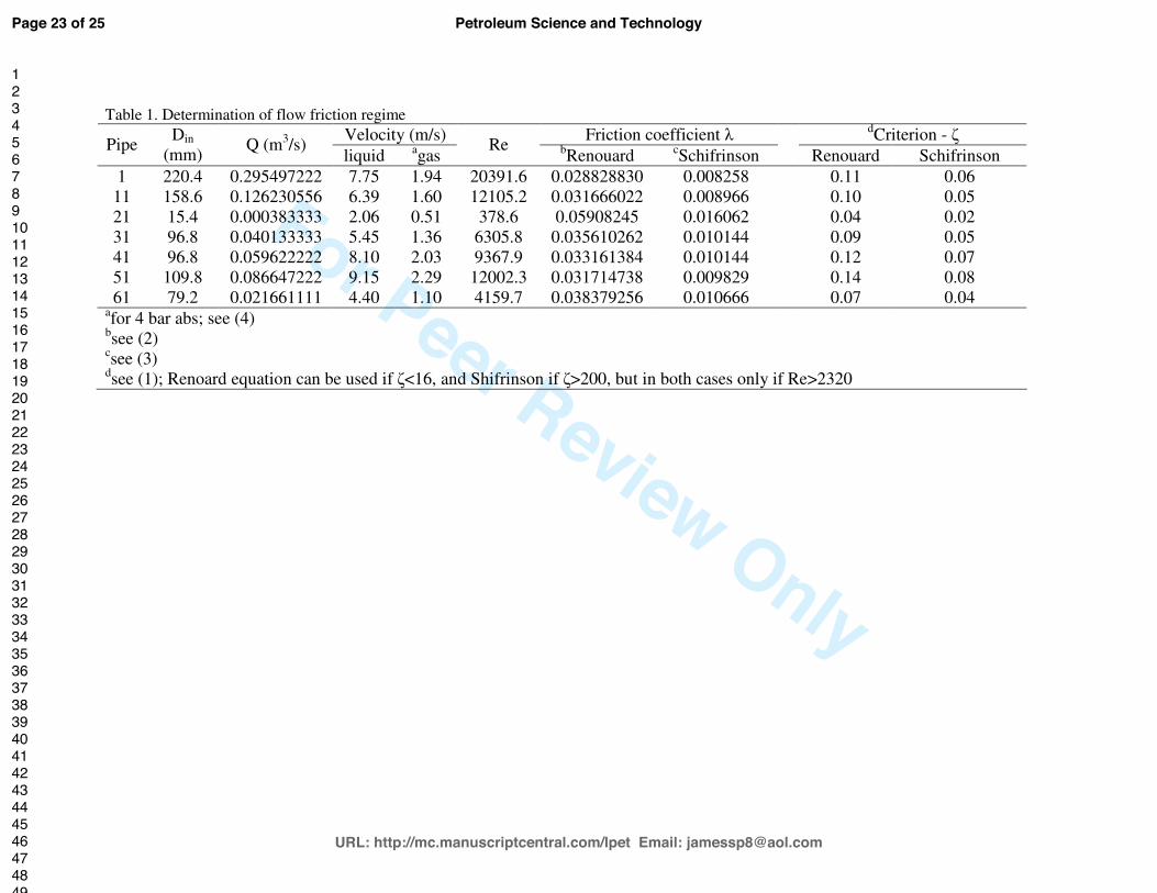
surface of polyethylene pipes is 000210-2 m To find which flow regime are occurred in
network it is necessary to find parameter ζ and hence every tenth pipes from network shown in
figure 3 are examined and results are listed in table 1
Table 1 Determination of flow friction regime
Results of random samples of pipes shown in table 1 concluded assumption that flow in
presented gas network is in hydraulically lsquosmoothrsquo regime because ζlt16 and hence Renouard
equation (2) is more suitable for this calculation Shifrinson equation (3) used previously in 1994
which is suitable for lsquoroughrsquo pipes cannot be used In some pipes such as 21 regime is not even
lsquosmoothrsquo it is rather laminar Velocity of gaseous fluids depends on the pressure in pipe since
they are compressible (4)
πsdot
sdot=
πsdotsdot
sdotsdot=
2in
2in
stst
D
Q4
Dp
Qp4v (4)
Page 7 of 25
URL httpmcmanuscriptcentralcomlpet Email jamessp8aolcom
Petroleum Science and Technology
123456789101112131415161718192021222324252627282930313233343536373839404142434445464748495051525354555657585960
For Peer Review Only
8
Assumption of gas compressibility means that it is compressed and forced to convey through
pipes but inside the pipeline system pressure drop of already compressed gas is small and hence
further changes in gas density can be neglected This is main difference between liquid and
incompressible flow According to this water flow in pipelines is liquid incompressible flow
while the gas flow is gaseous incompressible flow
Calculated Darcyrsquos friction factor after Shifrinson relation (3) used in 1994 is more than 3 times
smaller in comparisons to the results obtained using recommended Renouard equation (2)
(Figure 2)
Figure 2 Identification of the problem in a characteristic diagram
Previous results (Manojlović 1994) are not in correlation with diagram of Moody (1944)
Someone can conclude that bellow laminar and lsquosmoothrsquo regime or better to say bellow lines in
diagram of Moody which represent these regimes exist some other regimes (Figure 2) Of course
such regimes such as lsquosub-laminarrsquo or some kind of turbulent regime below hydraulically
lsquosmoothrsquo regime cannot exist (Figure 1)
3 General equation for fluid flow
Losses of energy or head (pressure) losses depend on the shape size and roughness of a channel
the velocity and viscosity of a fluid and they do not depend on the absolute pressure of the fluid
For gaseous fluids some law of thermodynamics also have to be included
Page 8 of 25
URL httpmcmanuscriptcentralcomlpet Email jamessp8aolcom
Petroleum Science and Technology
123456789101112131415161718192021222324252627282930313233343536373839404142434445464748495051525354555657585960
For Peer Review Only
9
31 General equation for liquid flow
Experiments show that in many cases pressure drop are approximately proportional to the square
of the velocity (5) Equation (5) is called the Darcy-Weisbach equation named after Henry
Darcy a French engineer of the nineteenth century and Julius Weisbach a German mining
engineer and the scientist of the same era
ρsdotsdotsdotλ=minus2
v
D
Lpp
2
in21 (5)
In previous equation velocity and gas density must be correlated since the gas is incompressible
fluid and hence for gas is more suitable equation in next form (6) because Qρ=Qstρst
st2
2st
5in
2
2
5in
21
Q8
D
LQ8
D
Lpp ρsdot
π
sdotsdotsdotλ=ρsdot
π
sdotsdotsdotλ=minus (6)
For example pressure drop using Darcy-Weisbach equation for liquid flow (6) in random set of
pipes chosen from gas network from Kragujevac is shown in table 2
Table 2 Pressure drops using Darcy-Weisbach equation for liquid flow
In (6) if flow rate Q is given for pressure in gas pipeline ie for 4105 abs and not for normal
conditions density also have to be adjusted for this existing value of pressure in pipeline
(volume of gas is four time smaller in 4105 then in 1105)
32 General equation for steady-state flow of gas
Density of gas can be noted as (7)
TRz
Mp
sdotsdotsdot
=ρ (7)
Page 9 of 25
URL httpmcmanuscriptcentralcomlpet Email jamessp8aolcom
Petroleum Science and Technology
123456789101112131415161718192021222324252627282930313233343536373839404142434445464748495051525354555657585960
For Peer Review Only
10
Considering the momentum equation applied to a portion of pipe length inside which flows a
compressible fluid with an average velocity for example natural gas and assuming steady state
conditions general equation for gas flow can be written as (8)
02
v
D
L
2
pp
TRz
M
2
v
D
dLdp
2
v
D
dLdp 2
2
in
22
21
avravr
2
1
22
in
2
1
2
1
2
1
2
in
=ρ∆
λ+minus
sdotsdot=ρλ+ρ=ρλ+ intintint int
(8)
In (9) flow can be used instead of velocity (8) and combined with (7) gives
( )2st
22st
22st
24in
2st2
st2
2st2
2
22
TRz
Mp
D
Q16
A
Q
A
Qv
sdotsdot
sdot
πsdot
sdot=ρ=ρ=ρ
(9)
Considering that gas density (see eq 7) at standard pressure conditions is equal as in average
pressure in pipeline (ρst=ρavr) and finally assuming that for perfect gas M=Mairρr general
equation for steady-state flow of gas can be written as (10)
stst
stair2st
25in
2st2
221
TRz
Mp
D
QL16pp
sdotsdotρsdotsdot
πsdot
sdot∆sdotλ=minus
(10)
This equation is rearranged by Renouard (1952) in very today well known equation (11)
824in
r821
st22
21
D
LQ4810ppC
ρsdotsdotsdot=minus=
(11)
Previous equation is correlated with Renouard equation used for calculation of Darcyrsquo friction
factor for hydraulically lsquosmoothrsquo regime (2) but with only difference in that the Darcyrsquos factor
do not need to be calculated as for equation (10) because it is already incorporated by setting of
appropriate coefficient and exponents in equation (11) Renouard (1952) assumed that dynamic
viscosity of natural gas is η=1075710-5 Pas factor of compressibility is z=1 and that pressure
and temperature in pipeline is actually standard temperature (Tst=Tavg=28815 K Pst=101325105
Pa) This means that by fixing the value of gas kinematic viscosity the density is also kept fixed
which is physically inaccurate when considering compressible gas flow at medium or high
Page 10 of 25
URL httpmcmanuscriptcentralcomlpet Email jamessp8aolcom
Petroleum Science and Technology
123456789101112131415161718192021222324252627282930313233343536373839404142434445464748495051525354555657585960
For Peer Review Only
11
pressure because the kinematic viscosity of gases is highly dependent upon pressure According
to this gas flow in city distribution network can be treated as incompressible like in Kragujevac
where pressure drops is minor and hence Renouard equation (11) can be used
Some other transformations of general equation for steady-state flow of gas are available in the
paper of Coelho and Pinho (2007)
4 Comparison of the actual and previous results
In figure 3 is shown rings-like part of the gas distribution network from one municipality of the
Serbian town of Kragujevac (Manojlović et al 1994) There are 29 independent nodes in the
ring-like network 43 branches belonging to rings with 25 branches mutual to the two rings The
total network gas supply input in node 1 is 23394 m3h
Figure 3 Gas-pipeline network in Kragujevac
Hardy Cross method procedure can give good results in design of a looped gas-pipeline network
of composite structure (Cross 1936 Corfield et al 1974 Brkić 2009b) Results in table 3 are
calculated for locked up diameters from previous calculation available in Manojlović et al
(1994) while flows are treated as variables In last two columns in table 3 optimization problem
take place where flows are locked up while diameters are variables Gas consumption per node is
presented in figure 3 in brackets and computation results using Renouardrsquos equation adjusted for
gas pipelines (11) are shown in Table 3
Page 11 of 25
URL httpmcmanuscriptcentralcomlpet Email jamessp8aolcom
Petroleum Science and Technology
123456789101112131415161718192021222324252627282930313233343536373839404142434445464748495051525354555657585960
For Peer Review Only
12
Table 3 Computational results for gas network in Kragujevac
The flow direction in branches15 and 16 is opposite to the flow direction shown in figure 3
The velocity limits are 6 ms for the pipes of small diameter (up to 90 mm) and 12 ms for the
pipes of large diameter (up to 225 mm) according to original project (Manojlović et al 1994)
But calculated velocities in each of the pipes do not reach even 3 ms For example velocity in
some of the pipes is higher than proposed only with assumption that gas is actually a liquid In
previous calculation fact that gas is actually compressed and hence that volume of gas is
decreased is neglected Hence mass of gas is constant but volume is decreased while gas
density is according to this increased According to this gas network is not nearly optimized and
for gas network with input pressure 4105 Pa abs ie 3105 Pa gauge all values of velocities are in
the ranges of proposed limits It is much different with liquid For example gas velocity in pipe 1
from table 1 is only 194 ms but in the case of water or crude oil equivalent volume of fluid
cannot be initially compressed and hence this observed liquid is forced to convey with increased
velocity For pipe 1 from table 1 this velocity for liquid flow is 775 ms
5 Optimized design of a gas-distribution pipeline network
In the problem of optimization of pipe diameters flow rates calculated in previously and shown
in table 3 are not any more treated as variable Results of optimization problem are shown in last
two columns in table 3 These flow rates in the next calculation will be locked up while the
pipes diameters will be treated as variable (12)
Page 12 of 25
URL httpmcmanuscriptcentralcomlpet Email jamessp8aolcom
Petroleum Science and Technology
123456789101112131415161718192021222324252627282930313233343536373839404142434445464748495051525354555657585960
For Peer Review Only
13
( )582in
r821
st
in
824in
r821
st
inin
22
21
D
LQ4810824
D
D
LQ4810
D
C
D
pp ρsdotsdotsdotsdotminus=
part
ρsdotsdotsdotpart
=partpart
=partminuspart
(12)
For example for the loop XIV from the network shown in figure 3 previous so called lsquolooprsquo
equation can be written as (13)
( )
( ) ( ) ( )( )
( )( )
( )( )
( )( )
sdot+
sdotminus
sdotminussdotρsdotsdotminus=
=part
∆+minusminuspart=
partpart
in58243
43st821
43
in58218
18st821
18
in58217
17st821
17r
XIV
434318181717
XIV
XIV
D
LQ
D
LQ
D
LQ4810824
D
DpDCDC
D
DC
(13)
Optimized design of a gas-distribution pipeline network for Kragujevac gas network is shown in
last two columns in table 3 This optimization is for average velocity of gas in network of 9 ms
Some pipes have very small diameters after optimization and hence after adoption of first larger
standard diameter calculation of flow distribution for these new standard diameters has to be
repeated
According to principles of the Hardy Cross method lsquolooprsquo equations ie condition after second
Kirchhoffrsquos law has to be fulfilled at the end of calculation These equations represent energy
continuity while the first Kirchhoffrsquos law represents mass continuity for nodes Mass continuity
has to be fulfilled in all iterations for all nodes without exceptions Diameter corrections are
calculated after (14)
( )( ) i
i
ii
D
DC
DCD
partpart
=∆
(14)
These corrections calculated for all particular loops from the Kragujevac gas network have to be
added to previous value of diameter according to algebraic scheme available in literature
Page 13 of 25
URL httpmcmanuscriptcentralcomlpet Email jamessp8aolcom
Petroleum Science and Technology
123456789101112131415161718192021222324252627282930313233343536373839404142434445464748495051525354555657585960
For Peer Review Only
14
(Corfield et al 1974 Brkić 2009b) Of course many more efficient methods than original Cross
(1936) method exist but this is not main subject of this article For example calculated flows
presented in fourth column in table 3 are obtained using the node-loop method (Boulos et al
2006) and result of optimization problem from the last two columns in table 4 are obtained using
improved Hardy Cross method (Boulos et al 2006 Brkić 2009b) In both mentioned method
matrix formulations are used which can be easily solved using MS Excel
6 Conclusions
Hardy Cross method procedure or similar improved sort of procedures can give good results in
design of a looped gas-pipeline network of composite structure According to the price and
velocity limits the optimal design can be predicted But all parameters such as friction factor
relation for calculation of pressure drop in pipes ie equation for calculation of gas flow must be
chosen in a very careful way Today distributive gas network is usually calculated using
Renouard equation for determination of gas flow and pressure drop value Inner surface of
polyethylene pipes which are almost always used in gas distribution networks are practically
smooth and hence flow regime in the typical network is hydraulically lsquosmoothrsquo Using of
inappropriate friction factor can lead to a paradoxical result ie calculated Darcyrsquos friction factor
can belong to nonexistent regimes such as lsquosub-laminarrsquo or turbulent regime which is bellow
hydraulically lsquosmoothrsquo This means that calculated Darcyrsquos friction factor are highly
underestimated Further using Darcy-Weisbach equation for liquid flow instead it modified
version for gaseous flow pressure drop are overestimated This leads to pseudo-accurate final
results After all visible error is occurred in numerical values of some parameters like velocity
in this case Velocities in network according to previous results are significantly larger than
Page 14 of 25
URL httpmcmanuscriptcentralcomlpet Email jamessp8aolcom
Petroleum Science and Technology
123456789101112131415161718192021222324252627282930313233343536373839404142434445464748495051525354555657585960
For Peer Review Only
15
expected Consequence is that diameters of pipes are too large for required amount of gas and
hence network is not optimal
In the project for gas pipeline in Serbian town Kragujevac from 1994 the Darcy-Weisbach
equation for liquid flow were used instead of modified Darcy-Weisbach equation for gaseous
flow accompanied with inappropriate usage of Shifrinson equation for full turbulent regime
which is typical for liquid flow in a steel pipes instead of some sort of Blasius or Prandtl form of
equations which are typical for flow of gas through polyethylene pipes which are used for
Kragujevac gas network
Hazen-Williams relation is frequently used for waterworks or sewerage systems (Boulos et al
2006) but not only inaccurate or better to say accurate in limit range the Hazen-Williams
equation is conceptually incorrect (Liou 1998) Even assumed that gas flow is incompressible in
municipality pipelines this relation cannot be used for such systems as gas-distribution
networks
References
Boulos PF Lansey KE and Karney BW 2006 Comprehensive Water Distribution Systems
Analysis Handbook for Engineers and Planners Hardback MWH Soft Inc
Brkić D 2009a Comments on lsquoSettling velocities of particulate systems 15 Velocities in
turbulent Newtonian flowsrsquo International Journal of Mineral Processing 92 (3-4)201-202
Brkić D 2009b An improvement of Hardy Cross method applied on looped spatial natural gas
distribution networks Applied Energy 86(7-8)1290-1300
Page 15 of 25
URL httpmcmanuscriptcentralcomlpet Email jamessp8aolcom
Petroleum Science and Technology
123456789101112131415161718192021222324252627282930313233343536373839404142434445464748495051525354555657585960
For Peer Review Only
16
Chen NH 1979 An explicit equation for friction factor in pipe Industrial and Engineering
Chemistry Fundamentals 18(3)296-297
Chen NH 1980 Comments on lsquoAn explicit equation for friction factor in pipesrsquo Industrial and
Engineering Chemistry Fundamentals 19(2)229ndash230
Coelho PM and Pinho C 2007 Considerations about equations for steady state flow in natural
gas pipelines Journal of the Brazilian Society of Mechanical Sciences and Engineering
29(3)262-273
Corfield G Hunt BE Ott RJ Binder GP and Vandaveer FE 1974 Distribution design
for increased demand In Segeler CG (Ed) Gas Engineers Handbook Industrial Press New
York NY pp 63ndash83
Cross H 1936 Analysis of flow in networks of conduits or conductors University of Illinois
Engineering Experimental Station Bulletin 286 34(22)3-29
Liou CP 1998 Limitation and proper use of the Hazen-Williams equation Journal of
Hydraulic Engineering ASCE 124(9)951-954
Manojlović V Arsenović M and Pajović V 1994 Optimized design of a gas-distribution
pipeline network Applied Energy 48(3)217-224
Mathews EH and Kohler PAJ 1995 A numerical optimization procedure for complex pipe
and duct network design International Journal of Numerical Methods for Heat amp Fluid Flow
5(5)445-457
Moody LF 1944 Friction factors for pipe flow Transactions of ASME 66(8)671-684
Nekrasov B 1969 Hydraulics for Aeronautical Engineers Moscow Mir publishers
Page 16 of 25
URL httpmcmanuscriptcentralcomlpet Email jamessp8aolcom
Petroleum Science and Technology
123456789101112131415161718192021222324252627282930313233343536373839404142434445464748495051525354555657585960
For Peer Review Only
17
Pretorius JJ Malan AG and Visser JA 2008 A flow network formulation for compressible
and incompressible flow International Journal of Numerical Methods for Heat amp Fluid Flow
18(2)185-201
Renouard P 1952 Nouvelle meacutethode pour le calcul des reacuteseaux mailleacutes de conduites de gaz
Communication au Congregraves du Graz in French
Schorle BJ Churchill SW and Shacham M 1980 Comments on lsquoAn explicit equation for
friction factor in pipesrsquo Industrial and Engineering Chemistry Fundamentals 19(2)228ndash229
Sukharev MG Karasevich AM Samoilov RV and Tverskoi IV 2005 Investigation of the
hydraulic resistance in polyethylene pipelines Journal of Engineering Physics and
Thermophysics 78(2)350-359
Page 17 of 25
URL httpmcmanuscriptcentralcomlpet Email jamessp8aolcom
Petroleum Science and Technology
123456789101112131415161718192021222324252627282930313233343536373839404142434445464748495051525354555657585960
For Peer Review Only
18
Figures
Figure 1 Physical description of flow regimes
Figure 2 Identification of the problem in a characteristic diagram
Figure 3 Gas-pipeline network in Kragujevac
Page 18 of 25
URL httpmcmanuscriptcentralcomlpet Email jamessp8aolcom
Petroleum Science and Technology
123456789101112131415161718192021222324252627282930313233343536373839404142434445464748495051525354555657585960
For Peer Review Only
19
Tables
Table 1 Determination of flow friction regime
Table 2 Pressure drops using Darcy-Weisbach equation for liquid flow
Table 3 Computational results for gas network in Kragujevac
Page 19 of 25
URL httpmcmanuscriptcentralcomlpet Email jamessp8aolcom
Petroleum Science and Technology
123456789101112131415161718192021222324252627282930313233343536373839404142434445464748495051525354555657585960
For Peer Review Only
Physical description of flow regimes
134x99mm (300 x 300 DPI)
Page 20 of 25
URL httpmcmanuscriptcentralcomlpet Email jamessp8aolcom
Petroleum Science and Technology
123456789101112131415161718192021222324252627282930313233343536373839404142434445464748495051525354555657585960
For Peer Review Only
Identification of the problem in a characteristic diagram
122x99mm (300 x 300 DPI)
Page 21 of 25
URL httpmcmanuscriptcentralcomlpet Email jamessp8aolcom
Petroleum Science and Technology
123456789101112131415161718192021222324252627282930313233343536373839404142434445464748495051525354555657585960
For Peer Review Only
Gas-pipeline network in Kragujevac
124x119mm (300 x 300 DPI)
Page 22 of 25
URL httpmcmanuscriptcentralcomlpet Email jamessp8aolcom
Petroleum Science and Technology
123456789101112131415161718192021222324252627282930313233343536373839404142434445464748495051525354555657585960
For Peer Review Only
Table 1 Determination of flow friction regime
Velocity (ms) Friction coefficient λ dCriterion - ζ Pipe
Din
(mm) Q (m3s)
liquid agas Re bRenouard cSchifrinson Renouard Schifrinson
1 2204 0295497222 775 194 203916 0028828830 0008258 011 006 11 1586 0126230556 639 160 121052 0031666022 0008966 010 005 21 154 0000383333 206 051 3786 005908245 0016062 004 002 31 968 0040133333 545 136 63058 0035610262 0010144 009 005 41 968 0059622222 810 203 93679 0033161384 0010144 012 007 51 1098 0086647222 915 229 120023 0031714738 0009829 014 008 61 792 0021661111 440 110 41597 0038379256 0010666 007 004
afor 4 bar abs see (4) bsee (2) csee (3) dsee (1) Renoard equation can be used if ζlt16 and Shifrinson if ζgt200 but in both cases only if Regt2320
Page 23 of 25
URL httpmcmanuscriptcentralcomlpet Email jamessp8aolcom
Petroleum Science and Technology
123456789101112131415161718192021222324252627282930313233343536373839404142434445464748495051525354555657585960
For Peer Review Only
Table 2 Pressure drops using Darcy-Weisbach equation for liquid flow aPressurre drop Pa
Pipe L (m) Renouard Schifrinson
1 84 27684 7930 11 119 40740 11535 21 212 144682 39332 31 115 52842 15052 41 278 262535 80307 51 78 79236 24557 61 383 150696 41878
ausing (5) or (6) and values from Table 1 gas density is ~084
Page 24 of 25
URL httpmcmanuscriptcentralcomlpet Email jamessp8aolcom
Petroleum Science and Technology
123456789101112131415161718192021222324252627282930313233343536373839404142434445464748495051525354555657585960
For Peer Review Only
Table 3 Computational results for gas network in Kragujevac
Optimized design Pipe number
Pipe diameter
(mm)
Pipe length
(m)
Flows (m3h)
Velocity (ms) aPipe diameter
(mm) Velocity (ms)
1 2204 84 103586 189 10428 842 2 2204 72 130354 237 10977 957 3 1982 170 91363 206 9134 968 4 1098 206 27028 198 4813 1032 5 1982 224 98713 222 9414 985 6 1982 37 96470 217 9685 909 7 1982 30 93450 210 9921 839 8 1762 35 54421 155 8223 712 9 1762 64 51302 146 8010 707 10 1586 34 48183 169 7791 702 11 1586 119 43448 153 6971 791 12 1586 154 42278 149 6883 789 13 440 639 2140 098 1924 511 14 352 268 685 049 1101 500 15 352 164 -752 -054 1077 573 16 440 276 -2535 -116 1923 606 17 274 363 052 006 559 147 18 1234 175 39043 227 6526 811 19 440 52 2534 116 2352 405 20 154 177 096 036 691 178 21 154 212 099 037 702 178 22 1098 161 28891 212 4757 1129 23 1234 108 26218 152 4977 936 24 554 194 3565 103 2344 574 25 968 135 14775 139 3842 885 26 274 215 269 032 902 292 27 1410 155 38654 172 6096 920 28 1586 34 60808 214 6978 1104 29 1586 48 54058 190 6925 997 30 1234 86 37663 219 5716 1019 31 968 115 14056 133 3721 898 32 352 75 1802 129 1463 744 33 554 70 7575 218 2600 991 34 968 102 19690 186 3638 1315 35 968 52 17983 170 3576 1243 36 352 104 1245 089 1235 722 37 968 101 15718 148 3432 1180 38 968 86 15635 148 4311 744 39 968 37 12051 114 3704 777 40 968 30 29739 281 5212 968 41 968 278 20027 189 3979 1118 42 968 115 23024 217 4688 926 43 1234 199 36724 213 5334 1141
afirst larger or smaller standard diameter have to be chosen
Page 25 of 25
URL httpmcmanuscriptcentralcomlpet Email jamessp8aolcom
Petroleum Science and Technology
123456789101112131415161718192021222324252627282930313233343536373839404142434445464748495051525354555657585960
Page 2
For Peer Review Only
Gas Distribution Network Hydraulic Problem from Practice
Journal Petroleum Science and Technology
Manuscript ID LPET-2009-0167
Manuscript Type Original Papers
Date Submitted by the Author
02-Jul-2009
Complete List of Authors Brkic Dejan Ministry of Science and Technological Development
Keywords natural gas gas distribution pipeline network flow friction hydraulic resistance
URL httpmcmanuscriptcentralcomlpet Email jamessp8aolcom
Petroleum Science and Technology
For Peer Review Only
1
Gas Distribution Network Hydraulic Problem from Practice
Abstract Accent is on determination of appropriate friction factor and on selection of
representative equation for natural gas flow under presented conditions in the network
Calculation of presented looped gas-pipeline network is done according to principles of Hardy
Cross method The final flows were calculated for known pipes diameters and nodes
consumptions while the flow velocities through pipes have to stand below certain values In
optimization problem flows are treated as constant while the diameters are variables
Keywords natural gas gas distribution pipeline network flow friction hydraulic resistance
Nomenclature
p-pressure (Pa)
λ-Darcy friction factor or coefficient (-)
L-length of pipe (m)
D-diameter of pipe (m)
v-velocity (ms)
ρ-density (kgm3)
Q-flow (m3s)
Re-Reynolds number (-)
η-gas dynamic viscosity (Pamiddots)
k-inside pipe wall roughness (m)
T-temperature (K)
z-gas compressibility factor (-)
Page 1 of 25
URL httpmcmanuscriptcentralcomlpet Email jamessp8aolcom
Petroleum Science and Technology
123456789101112131415161718192021222324252627282930313233343536373839404142434445464748495051525354555657585960
For Peer Review Only
2
M-relative molecular mass (-)
R-universal gas constant = 831441 J(kmolmiddotK)
τ-shear stress (Pa)
22
21 ppC minus=
Greek
ζ-parameter for existing of different turbulent regimes (ζlt16-rsquosmoothrsquo turbulent regime
16ltζlt200-partially turbulent ζgt200 fully turbulent regime)
π-Ludolphrsquos number (314159)
subscripts
1-beginning of pipe (accompanied with p)
2-end of pipe (accompanied with p)
in-inner
r-relative
st-at standard condition (Tst=28815 K pst=101325105 Pa)
avr-average
i-counter
-mark lsquolooprsquo or rsquocontourrsquo
Other signs
part-sign for lsquopartial differentialrsquo
d-infinitesimally small change of value
∆-definitive change of value
1 Introduction
Page 2 of 25
URL httpmcmanuscriptcentralcomlpet Email jamessp8aolcom
Petroleum Science and Technology
123456789101112131415161718192021222324252627282930313233343536373839404142434445464748495051525354555657585960
For Peer Review Only
3
When a gas is forced to flow through pipes it expands to a lower pressure and changes its
density Flow-rate ie pressure drop equations for condition in gas distribution networks
assumes a constant density of a fluid within the pipes This assumption applies only to
incompressible ie for liquids flows such as in water-distribution systems for municipalities (or
any other liquid like crude oil etc) For the small pressure drops in typical gas distribution
networks gas density can be treated as constant which means that gas can be treated as
incompressible fluid (Pretorius et al 2008) but not as liquid flow Liquid flow and
incompressible flow are not synonyms Under these circumstances flow equation for water or
crude oil cannot be literally copied and applied for natural gas flow This means that original
Darcy-Weisbach equation cannot be used without some modifications
Each pipe is connected to two nodes at its ends In a pipe network system pipes are the channels
used to convey fluid from one location to another The physical characteristics of a pipe include
the length inside diameter and roughness The Darcyrsquos coefficient of hydraulics resistance is
associated with the pipe material and age but also with fluid flow rate and pipe diameter ie
with relative roughness and Reynolds number When fluid is conveyed through the pipe
hydraulic energy is lost due to the friction between the moving fluid and the stationary pipe
surface This friction loss is a major energy loss in pipe flow and is a function of relative
roughness and Reynolds number as mentioned before In the case when the relative roughness is
negligible typical flow regime is hydraulically lsquosmoothrsquo where Darcyrsquos coefficient of hydraulics
resistances depend only on Reynolds number This regime is typical for gas networks which are
built using polyethylene pipes For that regime Darcyrsquos coefficient of hydraulics resistances can
be calculated after so called Blasius type equations or after so called Prandtl type of equations
Page 3 of 25
URL httpmcmanuscriptcentralcomlpet Email jamessp8aolcom
Petroleum Science and Technology
123456789101112131415161718192021222324252627282930313233343536373839404142434445464748495051525354555657585960
For Peer Review Only
4
Prandtl type of equations which is also known as NPK type (Nikuradse-Prandtl-von Karman) is
implicit in friction coefficient (Moody 1944 Coelho and Pinho 2007) For liquid flow where the
liquid density has larger values compared to gas Reynolds number increase and if it is
accompanied with increased value of relative roughness which is typical for steel pipes full
turbulent regime is most possible For the fully turbulent regime most convenient is von Karman
type of equation from western practice or Shifrinson equation from Russian practice For the
fully turbulent flow regime Darcyrsquos coefficient of hydraulics resistances depend only on relative
roughness
In this paper is shown new facts in comparison to previous calculation of gas distribution
network in Serbian town Kragujevac which was done in 1994 After the implementation
measurements in situ have performed and real measured values deviate from calculated Previous
results are available since they are published and hence comparisons are possible (Manojlović et
al 1994)
This paper addresses to the problem of hydraulic resistance in pipes used for construction of
networks for distribution of natural gas in the cities and with subject to all the practical
requirements for the engineers charged with design andor analysis of such system (Mathews and
Koumlhler 1995) This paper is especially addressed to those engineers willing to understand and
interpret the results of calculation properly and to make good engineering decision based on this
subject
2 On the Darcyrsquos coefficient of flow friction
Page 4 of 25
URL httpmcmanuscriptcentralcomlpet Email jamessp8aolcom
Petroleum Science and Technology
123456789101112131415161718192021222324252627282930313233343536373839404142434445464748495051525354555657585960
For Peer Review Only
5
To predict whether flow will be laminar hydraulically lsquosmoothrsquo partially turbulent or fully
turbulent it is necessary to explore the characteristics of flow (Figure 1) Hydraulically lsquosmoothrsquo
regime is also sort of turbulent regime In these considerations has to be very careful because
some of the authors use Darcyrsquos friction factor while the others use Fanningrsquos factor (Brkić
2009a) The Darcyrsquos friction coefficient is four times larger than Fanningrsquos while the physical
meaning is equal Graphically friction factor for known Reynolds number and relative roughness
can be determined using well known Moody diagram (Moody 1944) The Darcy friction factor
and the Moody friction factor are synonyms Note also that relative roughness is somewhere
defined using pipe diameter and somewhere using pipe radius which can be source of errors in
the caseof inappropriate use (Chen1979 Chen 1980 Schorle et al 1980 Brkić 2009a)
Figure 1 Physical description of flow regimes
Note that the Darcy friction factor is defined in theory as λ=(8τ)(ρv2)
As mentioned in introduction for polyethylene pipes absolute roughness k is very small
compared to the pipe diameter Din ie relative roughness is negligible (kDinrarr 0) and Darcyrsquos
friction coefficient depends only on Reynolds number For the low value of Reynolds number
but above 2320 flow regime is so called hydraulically lsquosmoothrsquo (there is no effect of roughness)
For the Reynolds number bellow 2320 regime is laminar Upper limit for hydraulically lsquosmoothrsquo
regime ζ=16 Typical partially turbulent regime is occurred for 16ltζlt200 and for ζgt200 fully
turbulent regime is most possible Parameter ζ can be found after (1)
Page 5 of 25
URL httpmcmanuscriptcentralcomlpet Email jamessp8aolcom
Petroleum Science and Technology
123456789101112131415161718192021222324252627282930313233343536373839404142434445464748495051525354555657585960
For Peer Review Only
6
inD
Rek λsdotsdot=ζ (1)
So as Reynolds number increases the flow becomes transitionally rough ie flow regime is
partially turbulent in which the friction factor rises above the lsquosmoothrsquo value and is a function of
both relative roughness and Reynolds number As Reynolds number increases more and more
the flow reaches a fully turbulent or so called lsquoroughrsquo regime in which the Darcyrsquos friction
coefficient is independent on Reynolds number and depends only on relative roughness In a
hydraulically lsquosmoothrsquo pipe flow the viscous sub-layer completely submerges the effect of
roughness on the flow For turbulent flow in lsquosmoothrsquo pipes friction losses are completely
determined by Reynolds number In rough pipes however the value of friction coefficient
depends for large values of Reynolds number also on the roughness of the inside pipe surface
The important point is not so much the absolute roughness size because for the same absolute
roughness the flow resistance in large pipe is considerably smaller than the resistance of a small
one
The Darcyrsquo friction factor for hydraulically lsquosmoothrsquo regime can be determined after Renouard
equation (3)
81Re
1720=λ (2)
This equation belongs to so called Blasius type of equations for hydraulically lsquosmoothrsquo regime
For fully turbulent regime from Russian literature (Sukharev et al 2005 Nekrasov 1969) is
available Shifrinson equation (3)
Page 6 of 25
URL httpmcmanuscriptcentralcomlpet Email jamessp8aolcom
Petroleum Science and Technology
123456789101112131415161718192021222324252627282930313233343536373839404142434445464748495051525354555657585960
For Peer Review Only
7
4
1
inD
k110
sdot=λ (3)
Shifrinson equation (3) was used for calculation of gas network in Kragujevac in 1994 In our
case for Kragujevac gas network gas dynamic viscosity is η=10758middot10-5 Pas which typical for
natural gas density of natural gas is 084 kgm-3 (that implies that relative density is 064) Value
of absolute roughness is 000710-3 m for the polyethylene pipes in Kragujevac as reported in the
paper of Manojlović et al (1994) which is even smaller compared to the value reported in the
paper of Sukharev et al (2005) Sukharev et al (2005) found that absolute roughness of inner
surface of polyethylene pipes is 000210-2 m To find which flow regime are occurred in
network it is necessary to find parameter ζ and hence every tenth pipes from network shown in
figure 3 are examined and results are listed in table 1
Table 1 Determination of flow friction regime
Results of random samples of pipes shown in table 1 concluded assumption that flow in
presented gas network is in hydraulically lsquosmoothrsquo regime because ζlt16 and hence Renouard
equation (2) is more suitable for this calculation Shifrinson equation (3) used previously in 1994
which is suitable for lsquoroughrsquo pipes cannot be used In some pipes such as 21 regime is not even
lsquosmoothrsquo it is rather laminar Velocity of gaseous fluids depends on the pressure in pipe since
they are compressible (4)
πsdot
sdot=
πsdotsdot
sdotsdot=
2in
2in
stst
D
Q4
Dp
Qp4v (4)
Page 7 of 25
URL httpmcmanuscriptcentralcomlpet Email jamessp8aolcom
Petroleum Science and Technology
123456789101112131415161718192021222324252627282930313233343536373839404142434445464748495051525354555657585960
For Peer Review Only
8
Assumption of gas compressibility means that it is compressed and forced to convey through
pipes but inside the pipeline system pressure drop of already compressed gas is small and hence
further changes in gas density can be neglected This is main difference between liquid and
incompressible flow According to this water flow in pipelines is liquid incompressible flow
while the gas flow is gaseous incompressible flow
Calculated Darcyrsquos friction factor after Shifrinson relation (3) used in 1994 is more than 3 times
smaller in comparisons to the results obtained using recommended Renouard equation (2)
(Figure 2)
Figure 2 Identification of the problem in a characteristic diagram
Previous results (Manojlović 1994) are not in correlation with diagram of Moody (1944)
Someone can conclude that bellow laminar and lsquosmoothrsquo regime or better to say bellow lines in
diagram of Moody which represent these regimes exist some other regimes (Figure 2) Of course
such regimes such as lsquosub-laminarrsquo or some kind of turbulent regime below hydraulically
lsquosmoothrsquo regime cannot exist (Figure 1)
3 General equation for fluid flow
Losses of energy or head (pressure) losses depend on the shape size and roughness of a channel
the velocity and viscosity of a fluid and they do not depend on the absolute pressure of the fluid
For gaseous fluids some law of thermodynamics also have to be included
Page 8 of 25
URL httpmcmanuscriptcentralcomlpet Email jamessp8aolcom
Petroleum Science and Technology
123456789101112131415161718192021222324252627282930313233343536373839404142434445464748495051525354555657585960
For Peer Review Only
9
31 General equation for liquid flow
Experiments show that in many cases pressure drop are approximately proportional to the square
of the velocity (5) Equation (5) is called the Darcy-Weisbach equation named after Henry
Darcy a French engineer of the nineteenth century and Julius Weisbach a German mining
engineer and the scientist of the same era
ρsdotsdotsdotλ=minus2
v
D
Lpp
2
in21 (5)
In previous equation velocity and gas density must be correlated since the gas is incompressible
fluid and hence for gas is more suitable equation in next form (6) because Qρ=Qstρst
st2
2st
5in
2
2
5in
21
Q8
D
LQ8
D
Lpp ρsdot
π
sdotsdotsdotλ=ρsdot
π
sdotsdotsdotλ=minus (6)
For example pressure drop using Darcy-Weisbach equation for liquid flow (6) in random set of
pipes chosen from gas network from Kragujevac is shown in table 2
Table 2 Pressure drops using Darcy-Weisbach equation for liquid flow
In (6) if flow rate Q is given for pressure in gas pipeline ie for 4105 abs and not for normal
conditions density also have to be adjusted for this existing value of pressure in pipeline
(volume of gas is four time smaller in 4105 then in 1105)
32 General equation for steady-state flow of gas
Density of gas can be noted as (7)
TRz
Mp
sdotsdotsdot
=ρ (7)
Page 9 of 25
URL httpmcmanuscriptcentralcomlpet Email jamessp8aolcom
Petroleum Science and Technology
123456789101112131415161718192021222324252627282930313233343536373839404142434445464748495051525354555657585960
For Peer Review Only
10
Considering the momentum equation applied to a portion of pipe length inside which flows a
compressible fluid with an average velocity for example natural gas and assuming steady state
conditions general equation for gas flow can be written as (8)
02
v
D
L
2
pp
TRz
M
2
v
D
dLdp
2
v
D
dLdp 2
2
in
22
21
avravr
2
1
22
in
2
1
2
1
2
1
2
in
=ρ∆
λ+minus
sdotsdot=ρλ+ρ=ρλ+ intintint int
(8)
In (9) flow can be used instead of velocity (8) and combined with (7) gives
( )2st
22st
22st
24in
2st2
st2
2st2
2
22
TRz
Mp
D
Q16
A
Q
A
Qv
sdotsdot
sdot
πsdot
sdot=ρ=ρ=ρ
(9)
Considering that gas density (see eq 7) at standard pressure conditions is equal as in average
pressure in pipeline (ρst=ρavr) and finally assuming that for perfect gas M=Mairρr general
equation for steady-state flow of gas can be written as (10)
stst
stair2st
25in
2st2
221
TRz
Mp
D
QL16pp
sdotsdotρsdotsdot
πsdot
sdot∆sdotλ=minus
(10)
This equation is rearranged by Renouard (1952) in very today well known equation (11)
824in
r821
st22
21
D
LQ4810ppC
ρsdotsdotsdot=minus=
(11)
Previous equation is correlated with Renouard equation used for calculation of Darcyrsquo friction
factor for hydraulically lsquosmoothrsquo regime (2) but with only difference in that the Darcyrsquos factor
do not need to be calculated as for equation (10) because it is already incorporated by setting of
appropriate coefficient and exponents in equation (11) Renouard (1952) assumed that dynamic
viscosity of natural gas is η=1075710-5 Pas factor of compressibility is z=1 and that pressure
and temperature in pipeline is actually standard temperature (Tst=Tavg=28815 K Pst=101325105
Pa) This means that by fixing the value of gas kinematic viscosity the density is also kept fixed
which is physically inaccurate when considering compressible gas flow at medium or high
Page 10 of 25
URL httpmcmanuscriptcentralcomlpet Email jamessp8aolcom
Petroleum Science and Technology
123456789101112131415161718192021222324252627282930313233343536373839404142434445464748495051525354555657585960
For Peer Review Only
11
pressure because the kinematic viscosity of gases is highly dependent upon pressure According
to this gas flow in city distribution network can be treated as incompressible like in Kragujevac
where pressure drops is minor and hence Renouard equation (11) can be used
Some other transformations of general equation for steady-state flow of gas are available in the
paper of Coelho and Pinho (2007)
4 Comparison of the actual and previous results
In figure 3 is shown rings-like part of the gas distribution network from one municipality of the
Serbian town of Kragujevac (Manojlović et al 1994) There are 29 independent nodes in the
ring-like network 43 branches belonging to rings with 25 branches mutual to the two rings The
total network gas supply input in node 1 is 23394 m3h
Figure 3 Gas-pipeline network in Kragujevac
Hardy Cross method procedure can give good results in design of a looped gas-pipeline network
of composite structure (Cross 1936 Corfield et al 1974 Brkić 2009b) Results in table 3 are
calculated for locked up diameters from previous calculation available in Manojlović et al
(1994) while flows are treated as variables In last two columns in table 3 optimization problem
take place where flows are locked up while diameters are variables Gas consumption per node is
presented in figure 3 in brackets and computation results using Renouardrsquos equation adjusted for
gas pipelines (11) are shown in Table 3
Page 11 of 25
URL httpmcmanuscriptcentralcomlpet Email jamessp8aolcom
Petroleum Science and Technology
123456789101112131415161718192021222324252627282930313233343536373839404142434445464748495051525354555657585960
For Peer Review Only
12
Table 3 Computational results for gas network in Kragujevac
The flow direction in branches15 and 16 is opposite to the flow direction shown in figure 3
The velocity limits are 6 ms for the pipes of small diameter (up to 90 mm) and 12 ms for the
pipes of large diameter (up to 225 mm) according to original project (Manojlović et al 1994)
But calculated velocities in each of the pipes do not reach even 3 ms For example velocity in
some of the pipes is higher than proposed only with assumption that gas is actually a liquid In
previous calculation fact that gas is actually compressed and hence that volume of gas is
decreased is neglected Hence mass of gas is constant but volume is decreased while gas
density is according to this increased According to this gas network is not nearly optimized and
for gas network with input pressure 4105 Pa abs ie 3105 Pa gauge all values of velocities are in
the ranges of proposed limits It is much different with liquid For example gas velocity in pipe 1
from table 1 is only 194 ms but in the case of water or crude oil equivalent volume of fluid
cannot be initially compressed and hence this observed liquid is forced to convey with increased
velocity For pipe 1 from table 1 this velocity for liquid flow is 775 ms
5 Optimized design of a gas-distribution pipeline network
In the problem of optimization of pipe diameters flow rates calculated in previously and shown
in table 3 are not any more treated as variable Results of optimization problem are shown in last
two columns in table 3 These flow rates in the next calculation will be locked up while the
pipes diameters will be treated as variable (12)
Page 12 of 25
URL httpmcmanuscriptcentralcomlpet Email jamessp8aolcom
Petroleum Science and Technology
123456789101112131415161718192021222324252627282930313233343536373839404142434445464748495051525354555657585960
For Peer Review Only
13
( )582in
r821
st
in
824in
r821
st
inin
22
21
D
LQ4810824
D
D
LQ4810
D
C
D
pp ρsdotsdotsdotsdotminus=
part
ρsdotsdotsdotpart
=partpart
=partminuspart
(12)
For example for the loop XIV from the network shown in figure 3 previous so called lsquolooprsquo
equation can be written as (13)
( )
( ) ( ) ( )( )
( )( )
( )( )
( )( )
sdot+
sdotminus
sdotminussdotρsdotsdotminus=
=part
∆+minusminuspart=
partpart
in58243
43st821
43
in58218
18st821
18
in58217
17st821
17r
XIV
434318181717
XIV
XIV
D
LQ
D
LQ
D
LQ4810824
D
DpDCDC
D
DC
(13)
Optimized design of a gas-distribution pipeline network for Kragujevac gas network is shown in
last two columns in table 3 This optimization is for average velocity of gas in network of 9 ms
Some pipes have very small diameters after optimization and hence after adoption of first larger
standard diameter calculation of flow distribution for these new standard diameters has to be
repeated
According to principles of the Hardy Cross method lsquolooprsquo equations ie condition after second
Kirchhoffrsquos law has to be fulfilled at the end of calculation These equations represent energy
continuity while the first Kirchhoffrsquos law represents mass continuity for nodes Mass continuity
has to be fulfilled in all iterations for all nodes without exceptions Diameter corrections are
calculated after (14)
( )( ) i
i
ii
D
DC
DCD
partpart
=∆
(14)
These corrections calculated for all particular loops from the Kragujevac gas network have to be
added to previous value of diameter according to algebraic scheme available in literature
Page 13 of 25
URL httpmcmanuscriptcentralcomlpet Email jamessp8aolcom
Petroleum Science and Technology
123456789101112131415161718192021222324252627282930313233343536373839404142434445464748495051525354555657585960
For Peer Review Only
14
(Corfield et al 1974 Brkić 2009b) Of course many more efficient methods than original Cross
(1936) method exist but this is not main subject of this article For example calculated flows
presented in fourth column in table 3 are obtained using the node-loop method (Boulos et al
2006) and result of optimization problem from the last two columns in table 4 are obtained using
improved Hardy Cross method (Boulos et al 2006 Brkić 2009b) In both mentioned method
matrix formulations are used which can be easily solved using MS Excel
6 Conclusions
Hardy Cross method procedure or similar improved sort of procedures can give good results in
design of a looped gas-pipeline network of composite structure According to the price and
velocity limits the optimal design can be predicted But all parameters such as friction factor
relation for calculation of pressure drop in pipes ie equation for calculation of gas flow must be
chosen in a very careful way Today distributive gas network is usually calculated using
Renouard equation for determination of gas flow and pressure drop value Inner surface of
polyethylene pipes which are almost always used in gas distribution networks are practically
smooth and hence flow regime in the typical network is hydraulically lsquosmoothrsquo Using of
inappropriate friction factor can lead to a paradoxical result ie calculated Darcyrsquos friction factor
can belong to nonexistent regimes such as lsquosub-laminarrsquo or turbulent regime which is bellow
hydraulically lsquosmoothrsquo This means that calculated Darcyrsquos friction factor are highly
underestimated Further using Darcy-Weisbach equation for liquid flow instead it modified
version for gaseous flow pressure drop are overestimated This leads to pseudo-accurate final
results After all visible error is occurred in numerical values of some parameters like velocity
in this case Velocities in network according to previous results are significantly larger than
Page 14 of 25
URL httpmcmanuscriptcentralcomlpet Email jamessp8aolcom
Petroleum Science and Technology
123456789101112131415161718192021222324252627282930313233343536373839404142434445464748495051525354555657585960
For Peer Review Only
15
expected Consequence is that diameters of pipes are too large for required amount of gas and
hence network is not optimal
In the project for gas pipeline in Serbian town Kragujevac from 1994 the Darcy-Weisbach
equation for liquid flow were used instead of modified Darcy-Weisbach equation for gaseous
flow accompanied with inappropriate usage of Shifrinson equation for full turbulent regime
which is typical for liquid flow in a steel pipes instead of some sort of Blasius or Prandtl form of
equations which are typical for flow of gas through polyethylene pipes which are used for
Kragujevac gas network
Hazen-Williams relation is frequently used for waterworks or sewerage systems (Boulos et al
2006) but not only inaccurate or better to say accurate in limit range the Hazen-Williams
equation is conceptually incorrect (Liou 1998) Even assumed that gas flow is incompressible in
municipality pipelines this relation cannot be used for such systems as gas-distribution
networks
References
Boulos PF Lansey KE and Karney BW 2006 Comprehensive Water Distribution Systems
Analysis Handbook for Engineers and Planners Hardback MWH Soft Inc
Brkić D 2009a Comments on lsquoSettling velocities of particulate systems 15 Velocities in
turbulent Newtonian flowsrsquo International Journal of Mineral Processing 92 (3-4)201-202
Brkić D 2009b An improvement of Hardy Cross method applied on looped spatial natural gas
distribution networks Applied Energy 86(7-8)1290-1300
Page 15 of 25
URL httpmcmanuscriptcentralcomlpet Email jamessp8aolcom
Petroleum Science and Technology
123456789101112131415161718192021222324252627282930313233343536373839404142434445464748495051525354555657585960
For Peer Review Only
16
Chen NH 1979 An explicit equation for friction factor in pipe Industrial and Engineering
Chemistry Fundamentals 18(3)296-297
Chen NH 1980 Comments on lsquoAn explicit equation for friction factor in pipesrsquo Industrial and
Engineering Chemistry Fundamentals 19(2)229ndash230
Coelho PM and Pinho C 2007 Considerations about equations for steady state flow in natural
gas pipelines Journal of the Brazilian Society of Mechanical Sciences and Engineering
29(3)262-273
Corfield G Hunt BE Ott RJ Binder GP and Vandaveer FE 1974 Distribution design
for increased demand In Segeler CG (Ed) Gas Engineers Handbook Industrial Press New
York NY pp 63ndash83
Cross H 1936 Analysis of flow in networks of conduits or conductors University of Illinois
Engineering Experimental Station Bulletin 286 34(22)3-29
Liou CP 1998 Limitation and proper use of the Hazen-Williams equation Journal of
Hydraulic Engineering ASCE 124(9)951-954
Manojlović V Arsenović M and Pajović V 1994 Optimized design of a gas-distribution
pipeline network Applied Energy 48(3)217-224
Mathews EH and Kohler PAJ 1995 A numerical optimization procedure for complex pipe
and duct network design International Journal of Numerical Methods for Heat amp Fluid Flow
5(5)445-457
Moody LF 1944 Friction factors for pipe flow Transactions of ASME 66(8)671-684
Nekrasov B 1969 Hydraulics for Aeronautical Engineers Moscow Mir publishers
Page 16 of 25
URL httpmcmanuscriptcentralcomlpet Email jamessp8aolcom
Petroleum Science and Technology
123456789101112131415161718192021222324252627282930313233343536373839404142434445464748495051525354555657585960
For Peer Review Only
17
Pretorius JJ Malan AG and Visser JA 2008 A flow network formulation for compressible
and incompressible flow International Journal of Numerical Methods for Heat amp Fluid Flow
18(2)185-201
Renouard P 1952 Nouvelle meacutethode pour le calcul des reacuteseaux mailleacutes de conduites de gaz
Communication au Congregraves du Graz in French
Schorle BJ Churchill SW and Shacham M 1980 Comments on lsquoAn explicit equation for
friction factor in pipesrsquo Industrial and Engineering Chemistry Fundamentals 19(2)228ndash229
Sukharev MG Karasevich AM Samoilov RV and Tverskoi IV 2005 Investigation of the
hydraulic resistance in polyethylene pipelines Journal of Engineering Physics and
Thermophysics 78(2)350-359
Page 17 of 25
URL httpmcmanuscriptcentralcomlpet Email jamessp8aolcom
Petroleum Science and Technology
123456789101112131415161718192021222324252627282930313233343536373839404142434445464748495051525354555657585960
For Peer Review Only
18
Figures
Figure 1 Physical description of flow regimes
Figure 2 Identification of the problem in a characteristic diagram
Figure 3 Gas-pipeline network in Kragujevac
Page 18 of 25
URL httpmcmanuscriptcentralcomlpet Email jamessp8aolcom
Petroleum Science and Technology
123456789101112131415161718192021222324252627282930313233343536373839404142434445464748495051525354555657585960
For Peer Review Only
19
Tables
Table 1 Determination of flow friction regime
Table 2 Pressure drops using Darcy-Weisbach equation for liquid flow
Table 3 Computational results for gas network in Kragujevac
Page 19 of 25
URL httpmcmanuscriptcentralcomlpet Email jamessp8aolcom
Petroleum Science and Technology
123456789101112131415161718192021222324252627282930313233343536373839404142434445464748495051525354555657585960
For Peer Review Only
Physical description of flow regimes
134x99mm (300 x 300 DPI)
Page 20 of 25
URL httpmcmanuscriptcentralcomlpet Email jamessp8aolcom
Petroleum Science and Technology
123456789101112131415161718192021222324252627282930313233343536373839404142434445464748495051525354555657585960
For Peer Review Only
Identification of the problem in a characteristic diagram
122x99mm (300 x 300 DPI)
Page 21 of 25
URL httpmcmanuscriptcentralcomlpet Email jamessp8aolcom
Petroleum Science and Technology
123456789101112131415161718192021222324252627282930313233343536373839404142434445464748495051525354555657585960
For Peer Review Only
Gas-pipeline network in Kragujevac
124x119mm (300 x 300 DPI)
Page 22 of 25
URL httpmcmanuscriptcentralcomlpet Email jamessp8aolcom
Petroleum Science and Technology
123456789101112131415161718192021222324252627282930313233343536373839404142434445464748495051525354555657585960
For Peer Review Only
Table 1 Determination of flow friction regime
Velocity (ms) Friction coefficient λ dCriterion - ζ Pipe
Din
(mm) Q (m3s)
liquid agas Re bRenouard cSchifrinson Renouard Schifrinson
1 2204 0295497222 775 194 203916 0028828830 0008258 011 006 11 1586 0126230556 639 160 121052 0031666022 0008966 010 005 21 154 0000383333 206 051 3786 005908245 0016062 004 002 31 968 0040133333 545 136 63058 0035610262 0010144 009 005 41 968 0059622222 810 203 93679 0033161384 0010144 012 007 51 1098 0086647222 915 229 120023 0031714738 0009829 014 008 61 792 0021661111 440 110 41597 0038379256 0010666 007 004
afor 4 bar abs see (4) bsee (2) csee (3) dsee (1) Renoard equation can be used if ζlt16 and Shifrinson if ζgt200 but in both cases only if Regt2320
Page 23 of 25
URL httpmcmanuscriptcentralcomlpet Email jamessp8aolcom
Petroleum Science and Technology
123456789101112131415161718192021222324252627282930313233343536373839404142434445464748495051525354555657585960
For Peer Review Only
Table 2 Pressure drops using Darcy-Weisbach equation for liquid flow aPressurre drop Pa
Pipe L (m) Renouard Schifrinson
1 84 27684 7930 11 119 40740 11535 21 212 144682 39332 31 115 52842 15052 41 278 262535 80307 51 78 79236 24557 61 383 150696 41878
ausing (5) or (6) and values from Table 1 gas density is ~084
Page 24 of 25
URL httpmcmanuscriptcentralcomlpet Email jamessp8aolcom
Petroleum Science and Technology
123456789101112131415161718192021222324252627282930313233343536373839404142434445464748495051525354555657585960
For Peer Review Only
Table 3 Computational results for gas network in Kragujevac
Optimized design Pipe number
Pipe diameter
(mm)
Pipe length
(m)
Flows (m3h)
Velocity (ms) aPipe diameter
(mm) Velocity (ms)
1 2204 84 103586 189 10428 842 2 2204 72 130354 237 10977 957 3 1982 170 91363 206 9134 968 4 1098 206 27028 198 4813 1032 5 1982 224 98713 222 9414 985 6 1982 37 96470 217 9685 909 7 1982 30 93450 210 9921 839 8 1762 35 54421 155 8223 712 9 1762 64 51302 146 8010 707 10 1586 34 48183 169 7791 702 11 1586 119 43448 153 6971 791 12 1586 154 42278 149 6883 789 13 440 639 2140 098 1924 511 14 352 268 685 049 1101 500 15 352 164 -752 -054 1077 573 16 440 276 -2535 -116 1923 606 17 274 363 052 006 559 147 18 1234 175 39043 227 6526 811 19 440 52 2534 116 2352 405 20 154 177 096 036 691 178 21 154 212 099 037 702 178 22 1098 161 28891 212 4757 1129 23 1234 108 26218 152 4977 936 24 554 194 3565 103 2344 574 25 968 135 14775 139 3842 885 26 274 215 269 032 902 292 27 1410 155 38654 172 6096 920 28 1586 34 60808 214 6978 1104 29 1586 48 54058 190 6925 997 30 1234 86 37663 219 5716 1019 31 968 115 14056 133 3721 898 32 352 75 1802 129 1463 744 33 554 70 7575 218 2600 991 34 968 102 19690 186 3638 1315 35 968 52 17983 170 3576 1243 36 352 104 1245 089 1235 722 37 968 101 15718 148 3432 1180 38 968 86 15635 148 4311 744 39 968 37 12051 114 3704 777 40 968 30 29739 281 5212 968 41 968 278 20027 189 3979 1118 42 968 115 23024 217 4688 926 43 1234 199 36724 213 5334 1141
afirst larger or smaller standard diameter have to be chosen
Page 25 of 25
URL httpmcmanuscriptcentralcomlpet Email jamessp8aolcom
Petroleum Science and Technology
123456789101112131415161718192021222324252627282930313233343536373839404142434445464748495051525354555657585960
Page 3
For Peer Review Only
1
Gas Distribution Network Hydraulic Problem from Practice
Abstract Accent is on determination of appropriate friction factor and on selection of
representative equation for natural gas flow under presented conditions in the network
Calculation of presented looped gas-pipeline network is done according to principles of Hardy
Cross method The final flows were calculated for known pipes diameters and nodes
consumptions while the flow velocities through pipes have to stand below certain values In
optimization problem flows are treated as constant while the diameters are variables
Keywords natural gas gas distribution pipeline network flow friction hydraulic resistance
Nomenclature
p-pressure (Pa)
λ-Darcy friction factor or coefficient (-)
L-length of pipe (m)
D-diameter of pipe (m)
v-velocity (ms)
ρ-density (kgm3)
Q-flow (m3s)
Re-Reynolds number (-)
η-gas dynamic viscosity (Pamiddots)
k-inside pipe wall roughness (m)
T-temperature (K)
z-gas compressibility factor (-)
Page 1 of 25
URL httpmcmanuscriptcentralcomlpet Email jamessp8aolcom
Petroleum Science and Technology
123456789101112131415161718192021222324252627282930313233343536373839404142434445464748495051525354555657585960
For Peer Review Only
2
M-relative molecular mass (-)
R-universal gas constant = 831441 J(kmolmiddotK)
τ-shear stress (Pa)
22
21 ppC minus=
Greek
ζ-parameter for existing of different turbulent regimes (ζlt16-rsquosmoothrsquo turbulent regime
16ltζlt200-partially turbulent ζgt200 fully turbulent regime)
π-Ludolphrsquos number (314159)
subscripts
1-beginning of pipe (accompanied with p)
2-end of pipe (accompanied with p)
in-inner
r-relative
st-at standard condition (Tst=28815 K pst=101325105 Pa)
avr-average
i-counter
-mark lsquolooprsquo or rsquocontourrsquo
Other signs
part-sign for lsquopartial differentialrsquo
d-infinitesimally small change of value
∆-definitive change of value
1 Introduction
Page 2 of 25
URL httpmcmanuscriptcentralcomlpet Email jamessp8aolcom
Petroleum Science and Technology
123456789101112131415161718192021222324252627282930313233343536373839404142434445464748495051525354555657585960
For Peer Review Only
3
When a gas is forced to flow through pipes it expands to a lower pressure and changes its
density Flow-rate ie pressure drop equations for condition in gas distribution networks
assumes a constant density of a fluid within the pipes This assumption applies only to
incompressible ie for liquids flows such as in water-distribution systems for municipalities (or
any other liquid like crude oil etc) For the small pressure drops in typical gas distribution
networks gas density can be treated as constant which means that gas can be treated as
incompressible fluid (Pretorius et al 2008) but not as liquid flow Liquid flow and
incompressible flow are not synonyms Under these circumstances flow equation for water or
crude oil cannot be literally copied and applied for natural gas flow This means that original
Darcy-Weisbach equation cannot be used without some modifications
Each pipe is connected to two nodes at its ends In a pipe network system pipes are the channels
used to convey fluid from one location to another The physical characteristics of a pipe include
the length inside diameter and roughness The Darcyrsquos coefficient of hydraulics resistance is
associated with the pipe material and age but also with fluid flow rate and pipe diameter ie
with relative roughness and Reynolds number When fluid is conveyed through the pipe
hydraulic energy is lost due to the friction between the moving fluid and the stationary pipe
surface This friction loss is a major energy loss in pipe flow and is a function of relative
roughness and Reynolds number as mentioned before In the case when the relative roughness is
negligible typical flow regime is hydraulically lsquosmoothrsquo where Darcyrsquos coefficient of hydraulics
resistances depend only on Reynolds number This regime is typical for gas networks which are
built using polyethylene pipes For that regime Darcyrsquos coefficient of hydraulics resistances can
be calculated after so called Blasius type equations or after so called Prandtl type of equations
Page 3 of 25
URL httpmcmanuscriptcentralcomlpet Email jamessp8aolcom
Petroleum Science and Technology
123456789101112131415161718192021222324252627282930313233343536373839404142434445464748495051525354555657585960
For Peer Review Only
4
Prandtl type of equations which is also known as NPK type (Nikuradse-Prandtl-von Karman) is
implicit in friction coefficient (Moody 1944 Coelho and Pinho 2007) For liquid flow where the
liquid density has larger values compared to gas Reynolds number increase and if it is
accompanied with increased value of relative roughness which is typical for steel pipes full
turbulent regime is most possible For the fully turbulent regime most convenient is von Karman
type of equation from western practice or Shifrinson equation from Russian practice For the
fully turbulent flow regime Darcyrsquos coefficient of hydraulics resistances depend only on relative
roughness
In this paper is shown new facts in comparison to previous calculation of gas distribution
network in Serbian town Kragujevac which was done in 1994 After the implementation
measurements in situ have performed and real measured values deviate from calculated Previous
results are available since they are published and hence comparisons are possible (Manojlović et
al 1994)
This paper addresses to the problem of hydraulic resistance in pipes used for construction of
networks for distribution of natural gas in the cities and with subject to all the practical
requirements for the engineers charged with design andor analysis of such system (Mathews and
Koumlhler 1995) This paper is especially addressed to those engineers willing to understand and
interpret the results of calculation properly and to make good engineering decision based on this
subject
2 On the Darcyrsquos coefficient of flow friction
Page 4 of 25
URL httpmcmanuscriptcentralcomlpet Email jamessp8aolcom
Petroleum Science and Technology
123456789101112131415161718192021222324252627282930313233343536373839404142434445464748495051525354555657585960
For Peer Review Only
5
To predict whether flow will be laminar hydraulically lsquosmoothrsquo partially turbulent or fully
turbulent it is necessary to explore the characteristics of flow (Figure 1) Hydraulically lsquosmoothrsquo
regime is also sort of turbulent regime In these considerations has to be very careful because
some of the authors use Darcyrsquos friction factor while the others use Fanningrsquos factor (Brkić
2009a) The Darcyrsquos friction coefficient is four times larger than Fanningrsquos while the physical
meaning is equal Graphically friction factor for known Reynolds number and relative roughness
can be determined using well known Moody diagram (Moody 1944) The Darcy friction factor
and the Moody friction factor are synonyms Note also that relative roughness is somewhere
defined using pipe diameter and somewhere using pipe radius which can be source of errors in
the caseof inappropriate use (Chen1979 Chen 1980 Schorle et al 1980 Brkić 2009a)
Figure 1 Physical description of flow regimes
Note that the Darcy friction factor is defined in theory as λ=(8τ)(ρv2)
As mentioned in introduction for polyethylene pipes absolute roughness k is very small
compared to the pipe diameter Din ie relative roughness is negligible (kDinrarr 0) and Darcyrsquos
friction coefficient depends only on Reynolds number For the low value of Reynolds number
but above 2320 flow regime is so called hydraulically lsquosmoothrsquo (there is no effect of roughness)
For the Reynolds number bellow 2320 regime is laminar Upper limit for hydraulically lsquosmoothrsquo
regime ζ=16 Typical partially turbulent regime is occurred for 16ltζlt200 and for ζgt200 fully
turbulent regime is most possible Parameter ζ can be found after (1)
Page 5 of 25
URL httpmcmanuscriptcentralcomlpet Email jamessp8aolcom
Petroleum Science and Technology
123456789101112131415161718192021222324252627282930313233343536373839404142434445464748495051525354555657585960
For Peer Review Only
6
inD
Rek λsdotsdot=ζ (1)
So as Reynolds number increases the flow becomes transitionally rough ie flow regime is
partially turbulent in which the friction factor rises above the lsquosmoothrsquo value and is a function of
both relative roughness and Reynolds number As Reynolds number increases more and more
the flow reaches a fully turbulent or so called lsquoroughrsquo regime in which the Darcyrsquos friction
coefficient is independent on Reynolds number and depends only on relative roughness In a
hydraulically lsquosmoothrsquo pipe flow the viscous sub-layer completely submerges the effect of
roughness on the flow For turbulent flow in lsquosmoothrsquo pipes friction losses are completely
determined by Reynolds number In rough pipes however the value of friction coefficient
depends for large values of Reynolds number also on the roughness of the inside pipe surface
The important point is not so much the absolute roughness size because for the same absolute
roughness the flow resistance in large pipe is considerably smaller than the resistance of a small
one
The Darcyrsquo friction factor for hydraulically lsquosmoothrsquo regime can be determined after Renouard
equation (3)
81Re
1720=λ (2)
This equation belongs to so called Blasius type of equations for hydraulically lsquosmoothrsquo regime
For fully turbulent regime from Russian literature (Sukharev et al 2005 Nekrasov 1969) is
available Shifrinson equation (3)
Page 6 of 25
URL httpmcmanuscriptcentralcomlpet Email jamessp8aolcom
Petroleum Science and Technology
123456789101112131415161718192021222324252627282930313233343536373839404142434445464748495051525354555657585960
For Peer Review Only
7
4
1
inD
k110
sdot=λ (3)
Shifrinson equation (3) was used for calculation of gas network in Kragujevac in 1994 In our
case for Kragujevac gas network gas dynamic viscosity is η=10758middot10-5 Pas which typical for
natural gas density of natural gas is 084 kgm-3 (that implies that relative density is 064) Value
of absolute roughness is 000710-3 m for the polyethylene pipes in Kragujevac as reported in the
paper of Manojlović et al (1994) which is even smaller compared to the value reported in the
paper of Sukharev et al (2005) Sukharev et al (2005) found that absolute roughness of inner
surface of polyethylene pipes is 000210-2 m To find which flow regime are occurred in
network it is necessary to find parameter ζ and hence every tenth pipes from network shown in
figure 3 are examined and results are listed in table 1
Table 1 Determination of flow friction regime
Results of random samples of pipes shown in table 1 concluded assumption that flow in
presented gas network is in hydraulically lsquosmoothrsquo regime because ζlt16 and hence Renouard
equation (2) is more suitable for this calculation Shifrinson equation (3) used previously in 1994
which is suitable for lsquoroughrsquo pipes cannot be used In some pipes such as 21 regime is not even
lsquosmoothrsquo it is rather laminar Velocity of gaseous fluids depends on the pressure in pipe since
they are compressible (4)
πsdot
sdot=
πsdotsdot
sdotsdot=
2in
2in
stst
D
Q4
Dp
Qp4v (4)
Page 7 of 25
URL httpmcmanuscriptcentralcomlpet Email jamessp8aolcom
Petroleum Science and Technology
123456789101112131415161718192021222324252627282930313233343536373839404142434445464748495051525354555657585960
For Peer Review Only
8
Assumption of gas compressibility means that it is compressed and forced to convey through
pipes but inside the pipeline system pressure drop of already compressed gas is small and hence
further changes in gas density can be neglected This is main difference between liquid and
incompressible flow According to this water flow in pipelines is liquid incompressible flow
while the gas flow is gaseous incompressible flow
Calculated Darcyrsquos friction factor after Shifrinson relation (3) used in 1994 is more than 3 times
smaller in comparisons to the results obtained using recommended Renouard equation (2)
(Figure 2)
Figure 2 Identification of the problem in a characteristic diagram
Previous results (Manojlović 1994) are not in correlation with diagram of Moody (1944)
Someone can conclude that bellow laminar and lsquosmoothrsquo regime or better to say bellow lines in
diagram of Moody which represent these regimes exist some other regimes (Figure 2) Of course
such regimes such as lsquosub-laminarrsquo or some kind of turbulent regime below hydraulically
lsquosmoothrsquo regime cannot exist (Figure 1)
3 General equation for fluid flow
Losses of energy or head (pressure) losses depend on the shape size and roughness of a channel
the velocity and viscosity of a fluid and they do not depend on the absolute pressure of the fluid
For gaseous fluids some law of thermodynamics also have to be included
Page 8 of 25
URL httpmcmanuscriptcentralcomlpet Email jamessp8aolcom
Petroleum Science and Technology
123456789101112131415161718192021222324252627282930313233343536373839404142434445464748495051525354555657585960
For Peer Review Only
9
31 General equation for liquid flow
Experiments show that in many cases pressure drop are approximately proportional to the square
of the velocity (5) Equation (5) is called the Darcy-Weisbach equation named after Henry
Darcy a French engineer of the nineteenth century and Julius Weisbach a German mining
engineer and the scientist of the same era
ρsdotsdotsdotλ=minus2
v
D
Lpp
2
in21 (5)
In previous equation velocity and gas density must be correlated since the gas is incompressible
fluid and hence for gas is more suitable equation in next form (6) because Qρ=Qstρst
st2
2st
5in
2
2
5in
21
Q8
D
LQ8
D
Lpp ρsdot
π
sdotsdotsdotλ=ρsdot
π
sdotsdotsdotλ=minus (6)
For example pressure drop using Darcy-Weisbach equation for liquid flow (6) in random set of
pipes chosen from gas network from Kragujevac is shown in table 2
Table 2 Pressure drops using Darcy-Weisbach equation for liquid flow
In (6) if flow rate Q is given for pressure in gas pipeline ie for 4105 abs and not for normal
conditions density also have to be adjusted for this existing value of pressure in pipeline
(volume of gas is four time smaller in 4105 then in 1105)
32 General equation for steady-state flow of gas
Density of gas can be noted as (7)
TRz
Mp
sdotsdotsdot
=ρ (7)
Page 9 of 25
URL httpmcmanuscriptcentralcomlpet Email jamessp8aolcom
Petroleum Science and Technology
123456789101112131415161718192021222324252627282930313233343536373839404142434445464748495051525354555657585960
For Peer Review Only
10
Considering the momentum equation applied to a portion of pipe length inside which flows a
compressible fluid with an average velocity for example natural gas and assuming steady state
conditions general equation for gas flow can be written as (8)
02
v
D
L
2
pp
TRz
M
2
v
D
dLdp
2
v
D
dLdp 2
2
in
22
21
avravr
2
1
22
in
2
1
2
1
2
1
2
in
=ρ∆
λ+minus
sdotsdot=ρλ+ρ=ρλ+ intintint int
(8)
In (9) flow can be used instead of velocity (8) and combined with (7) gives
( )2st
22st
22st
24in
2st2
st2
2st2
2
22
TRz
Mp
D
Q16
A
Q
A
Qv
sdotsdot
sdot
πsdot
sdot=ρ=ρ=ρ
(9)
Considering that gas density (see eq 7) at standard pressure conditions is equal as in average
pressure in pipeline (ρst=ρavr) and finally assuming that for perfect gas M=Mairρr general
equation for steady-state flow of gas can be written as (10)
stst
stair2st
25in
2st2
221
TRz
Mp
D
QL16pp
sdotsdotρsdotsdot
πsdot
sdot∆sdotλ=minus
(10)
This equation is rearranged by Renouard (1952) in very today well known equation (11)
824in
r821
st22
21
D
LQ4810ppC
ρsdotsdotsdot=minus=
(11)
Previous equation is correlated with Renouard equation used for calculation of Darcyrsquo friction
factor for hydraulically lsquosmoothrsquo regime (2) but with only difference in that the Darcyrsquos factor
do not need to be calculated as for equation (10) because it is already incorporated by setting of
appropriate coefficient and exponents in equation (11) Renouard (1952) assumed that dynamic
viscosity of natural gas is η=1075710-5 Pas factor of compressibility is z=1 and that pressure
and temperature in pipeline is actually standard temperature (Tst=Tavg=28815 K Pst=101325105
Pa) This means that by fixing the value of gas kinematic viscosity the density is also kept fixed
which is physically inaccurate when considering compressible gas flow at medium or high
Page 10 of 25
URL httpmcmanuscriptcentralcomlpet Email jamessp8aolcom
Petroleum Science and Technology
123456789101112131415161718192021222324252627282930313233343536373839404142434445464748495051525354555657585960
For Peer Review Only
11
pressure because the kinematic viscosity of gases is highly dependent upon pressure According
to this gas flow in city distribution network can be treated as incompressible like in Kragujevac
where pressure drops is minor and hence Renouard equation (11) can be used
Some other transformations of general equation for steady-state flow of gas are available in the
paper of Coelho and Pinho (2007)
4 Comparison of the actual and previous results
In figure 3 is shown rings-like part of the gas distribution network from one municipality of the
Serbian town of Kragujevac (Manojlović et al 1994) There are 29 independent nodes in the
ring-like network 43 branches belonging to rings with 25 branches mutual to the two rings The
total network gas supply input in node 1 is 23394 m3h
Figure 3 Gas-pipeline network in Kragujevac
Hardy Cross method procedure can give good results in design of a looped gas-pipeline network
of composite structure (Cross 1936 Corfield et al 1974 Brkić 2009b) Results in table 3 are
calculated for locked up diameters from previous calculation available in Manojlović et al
(1994) while flows are treated as variables In last two columns in table 3 optimization problem
take place where flows are locked up while diameters are variables Gas consumption per node is
presented in figure 3 in brackets and computation results using Renouardrsquos equation adjusted for
gas pipelines (11) are shown in Table 3
Page 11 of 25
URL httpmcmanuscriptcentralcomlpet Email jamessp8aolcom
Petroleum Science and Technology
123456789101112131415161718192021222324252627282930313233343536373839404142434445464748495051525354555657585960
For Peer Review Only
12
Table 3 Computational results for gas network in Kragujevac
The flow direction in branches15 and 16 is opposite to the flow direction shown in figure 3
The velocity limits are 6 ms for the pipes of small diameter (up to 90 mm) and 12 ms for the
pipes of large diameter (up to 225 mm) according to original project (Manojlović et al 1994)
But calculated velocities in each of the pipes do not reach even 3 ms For example velocity in
some of the pipes is higher than proposed only with assumption that gas is actually a liquid In
previous calculation fact that gas is actually compressed and hence that volume of gas is
decreased is neglected Hence mass of gas is constant but volume is decreased while gas
density is according to this increased According to this gas network is not nearly optimized and
for gas network with input pressure 4105 Pa abs ie 3105 Pa gauge all values of velocities are in
the ranges of proposed limits It is much different with liquid For example gas velocity in pipe 1
from table 1 is only 194 ms but in the case of water or crude oil equivalent volume of fluid
cannot be initially compressed and hence this observed liquid is forced to convey with increased
velocity For pipe 1 from table 1 this velocity for liquid flow is 775 ms
5 Optimized design of a gas-distribution pipeline network
In the problem of optimization of pipe diameters flow rates calculated in previously and shown
in table 3 are not any more treated as variable Results of optimization problem are shown in last
two columns in table 3 These flow rates in the next calculation will be locked up while the
pipes diameters will be treated as variable (12)
Page 12 of 25
URL httpmcmanuscriptcentralcomlpet Email jamessp8aolcom
Petroleum Science and Technology
123456789101112131415161718192021222324252627282930313233343536373839404142434445464748495051525354555657585960
For Peer Review Only
13
( )582in
r821
st
in
824in
r821
st
inin
22
21
D
LQ4810824
D
D
LQ4810
D
C
D
pp ρsdotsdotsdotsdotminus=
part
ρsdotsdotsdotpart
=partpart
=partminuspart
(12)
For example for the loop XIV from the network shown in figure 3 previous so called lsquolooprsquo
equation can be written as (13)
( )
( ) ( ) ( )( )
( )( )
( )( )
( )( )
sdot+
sdotminus
sdotminussdotρsdotsdotminus=
=part
∆+minusminuspart=
partpart
in58243
43st821
43
in58218
18st821
18
in58217
17st821
17r
XIV
434318181717
XIV
XIV
D
LQ
D
LQ
D
LQ4810824
D
DpDCDC
D
DC
(13)
Optimized design of a gas-distribution pipeline network for Kragujevac gas network is shown in
last two columns in table 3 This optimization is for average velocity of gas in network of 9 ms
Some pipes have very small diameters after optimization and hence after adoption of first larger
standard diameter calculation of flow distribution for these new standard diameters has to be
repeated
According to principles of the Hardy Cross method lsquolooprsquo equations ie condition after second
Kirchhoffrsquos law has to be fulfilled at the end of calculation These equations represent energy
continuity while the first Kirchhoffrsquos law represents mass continuity for nodes Mass continuity
has to be fulfilled in all iterations for all nodes without exceptions Diameter corrections are
calculated after (14)
( )( ) i
i
ii
D
DC
DCD
partpart
=∆
(14)
These corrections calculated for all particular loops from the Kragujevac gas network have to be
added to previous value of diameter according to algebraic scheme available in literature
Page 13 of 25
URL httpmcmanuscriptcentralcomlpet Email jamessp8aolcom
Petroleum Science and Technology
123456789101112131415161718192021222324252627282930313233343536373839404142434445464748495051525354555657585960
For Peer Review Only
14
(Corfield et al 1974 Brkić 2009b) Of course many more efficient methods than original Cross
(1936) method exist but this is not main subject of this article For example calculated flows
presented in fourth column in table 3 are obtained using the node-loop method (Boulos et al
2006) and result of optimization problem from the last two columns in table 4 are obtained using
improved Hardy Cross method (Boulos et al 2006 Brkić 2009b) In both mentioned method
matrix formulations are used which can be easily solved using MS Excel
6 Conclusions
Hardy Cross method procedure or similar improved sort of procedures can give good results in
design of a looped gas-pipeline network of composite structure According to the price and
velocity limits the optimal design can be predicted But all parameters such as friction factor
relation for calculation of pressure drop in pipes ie equation for calculation of gas flow must be
chosen in a very careful way Today distributive gas network is usually calculated using
Renouard equation for determination of gas flow and pressure drop value Inner surface of
polyethylene pipes which are almost always used in gas distribution networks are practically
smooth and hence flow regime in the typical network is hydraulically lsquosmoothrsquo Using of
inappropriate friction factor can lead to a paradoxical result ie calculated Darcyrsquos friction factor
can belong to nonexistent regimes such as lsquosub-laminarrsquo or turbulent regime which is bellow
hydraulically lsquosmoothrsquo This means that calculated Darcyrsquos friction factor are highly
underestimated Further using Darcy-Weisbach equation for liquid flow instead it modified
version for gaseous flow pressure drop are overestimated This leads to pseudo-accurate final
results After all visible error is occurred in numerical values of some parameters like velocity
in this case Velocities in network according to previous results are significantly larger than
Page 14 of 25
URL httpmcmanuscriptcentralcomlpet Email jamessp8aolcom
Petroleum Science and Technology
123456789101112131415161718192021222324252627282930313233343536373839404142434445464748495051525354555657585960
For Peer Review Only
15
expected Consequence is that diameters of pipes are too large for required amount of gas and
hence network is not optimal
In the project for gas pipeline in Serbian town Kragujevac from 1994 the Darcy-Weisbach
equation for liquid flow were used instead of modified Darcy-Weisbach equation for gaseous
flow accompanied with inappropriate usage of Shifrinson equation for full turbulent regime
which is typical for liquid flow in a steel pipes instead of some sort of Blasius or Prandtl form of
equations which are typical for flow of gas through polyethylene pipes which are used for
Kragujevac gas network
Hazen-Williams relation is frequently used for waterworks or sewerage systems (Boulos et al
2006) but not only inaccurate or better to say accurate in limit range the Hazen-Williams
equation is conceptually incorrect (Liou 1998) Even assumed that gas flow is incompressible in
municipality pipelines this relation cannot be used for such systems as gas-distribution
networks
References
Boulos PF Lansey KE and Karney BW 2006 Comprehensive Water Distribution Systems
Analysis Handbook for Engineers and Planners Hardback MWH Soft Inc
Brkić D 2009a Comments on lsquoSettling velocities of particulate systems 15 Velocities in
turbulent Newtonian flowsrsquo International Journal of Mineral Processing 92 (3-4)201-202
Brkić D 2009b An improvement of Hardy Cross method applied on looped spatial natural gas
distribution networks Applied Energy 86(7-8)1290-1300
Page 15 of 25
URL httpmcmanuscriptcentralcomlpet Email jamessp8aolcom
Petroleum Science and Technology
123456789101112131415161718192021222324252627282930313233343536373839404142434445464748495051525354555657585960
For Peer Review Only
16
Chen NH 1979 An explicit equation for friction factor in pipe Industrial and Engineering
Chemistry Fundamentals 18(3)296-297
Chen NH 1980 Comments on lsquoAn explicit equation for friction factor in pipesrsquo Industrial and
Engineering Chemistry Fundamentals 19(2)229ndash230
Coelho PM and Pinho C 2007 Considerations about equations for steady state flow in natural
gas pipelines Journal of the Brazilian Society of Mechanical Sciences and Engineering
29(3)262-273
Corfield G Hunt BE Ott RJ Binder GP and Vandaveer FE 1974 Distribution design
for increased demand In Segeler CG (Ed) Gas Engineers Handbook Industrial Press New
York NY pp 63ndash83
Cross H 1936 Analysis of flow in networks of conduits or conductors University of Illinois
Engineering Experimental Station Bulletin 286 34(22)3-29
Liou CP 1998 Limitation and proper use of the Hazen-Williams equation Journal of
Hydraulic Engineering ASCE 124(9)951-954
Manojlović V Arsenović M and Pajović V 1994 Optimized design of a gas-distribution
pipeline network Applied Energy 48(3)217-224
Mathews EH and Kohler PAJ 1995 A numerical optimization procedure for complex pipe
and duct network design International Journal of Numerical Methods for Heat amp Fluid Flow
5(5)445-457
Moody LF 1944 Friction factors for pipe flow Transactions of ASME 66(8)671-684
Nekrasov B 1969 Hydraulics for Aeronautical Engineers Moscow Mir publishers
Page 16 of 25
URL httpmcmanuscriptcentralcomlpet Email jamessp8aolcom
Petroleum Science and Technology
123456789101112131415161718192021222324252627282930313233343536373839404142434445464748495051525354555657585960
For Peer Review Only
17
Pretorius JJ Malan AG and Visser JA 2008 A flow network formulation for compressible
and incompressible flow International Journal of Numerical Methods for Heat amp Fluid Flow
18(2)185-201
Renouard P 1952 Nouvelle meacutethode pour le calcul des reacuteseaux mailleacutes de conduites de gaz
Communication au Congregraves du Graz in French
Schorle BJ Churchill SW and Shacham M 1980 Comments on lsquoAn explicit equation for
friction factor in pipesrsquo Industrial and Engineering Chemistry Fundamentals 19(2)228ndash229
Sukharev MG Karasevich AM Samoilov RV and Tverskoi IV 2005 Investigation of the
hydraulic resistance in polyethylene pipelines Journal of Engineering Physics and
Thermophysics 78(2)350-359
Page 17 of 25
URL httpmcmanuscriptcentralcomlpet Email jamessp8aolcom
Petroleum Science and Technology
123456789101112131415161718192021222324252627282930313233343536373839404142434445464748495051525354555657585960
For Peer Review Only
18
Figures
Figure 1 Physical description of flow regimes
Figure 2 Identification of the problem in a characteristic diagram
Figure 3 Gas-pipeline network in Kragujevac
Page 18 of 25
URL httpmcmanuscriptcentralcomlpet Email jamessp8aolcom
Petroleum Science and Technology
123456789101112131415161718192021222324252627282930313233343536373839404142434445464748495051525354555657585960
For Peer Review Only
19
Tables
Table 1 Determination of flow friction regime
Table 2 Pressure drops using Darcy-Weisbach equation for liquid flow
Table 3 Computational results for gas network in Kragujevac
Page 19 of 25
URL httpmcmanuscriptcentralcomlpet Email jamessp8aolcom
Petroleum Science and Technology
123456789101112131415161718192021222324252627282930313233343536373839404142434445464748495051525354555657585960
For Peer Review Only
Physical description of flow regimes
134x99mm (300 x 300 DPI)
Page 20 of 25
URL httpmcmanuscriptcentralcomlpet Email jamessp8aolcom
Petroleum Science and Technology
123456789101112131415161718192021222324252627282930313233343536373839404142434445464748495051525354555657585960
For Peer Review Only
Identification of the problem in a characteristic diagram
122x99mm (300 x 300 DPI)
Page 21 of 25
URL httpmcmanuscriptcentralcomlpet Email jamessp8aolcom
Petroleum Science and Technology
123456789101112131415161718192021222324252627282930313233343536373839404142434445464748495051525354555657585960
For Peer Review Only
Gas-pipeline network in Kragujevac
124x119mm (300 x 300 DPI)
Page 22 of 25
URL httpmcmanuscriptcentralcomlpet Email jamessp8aolcom
Petroleum Science and Technology
123456789101112131415161718192021222324252627282930313233343536373839404142434445464748495051525354555657585960
For Peer Review Only
Table 1 Determination of flow friction regime
Velocity (ms) Friction coefficient λ dCriterion - ζ Pipe
Din
(mm) Q (m3s)
liquid agas Re bRenouard cSchifrinson Renouard Schifrinson
1 2204 0295497222 775 194 203916 0028828830 0008258 011 006 11 1586 0126230556 639 160 121052 0031666022 0008966 010 005 21 154 0000383333 206 051 3786 005908245 0016062 004 002 31 968 0040133333 545 136 63058 0035610262 0010144 009 005 41 968 0059622222 810 203 93679 0033161384 0010144 012 007 51 1098 0086647222 915 229 120023 0031714738 0009829 014 008 61 792 0021661111 440 110 41597 0038379256 0010666 007 004
afor 4 bar abs see (4) bsee (2) csee (3) dsee (1) Renoard equation can be used if ζlt16 and Shifrinson if ζgt200 but in both cases only if Regt2320
Page 23 of 25
URL httpmcmanuscriptcentralcomlpet Email jamessp8aolcom
Petroleum Science and Technology
123456789101112131415161718192021222324252627282930313233343536373839404142434445464748495051525354555657585960
For Peer Review Only
Table 2 Pressure drops using Darcy-Weisbach equation for liquid flow aPressurre drop Pa
Pipe L (m) Renouard Schifrinson
1 84 27684 7930 11 119 40740 11535 21 212 144682 39332 31 115 52842 15052 41 278 262535 80307 51 78 79236 24557 61 383 150696 41878
ausing (5) or (6) and values from Table 1 gas density is ~084
Page 24 of 25
URL httpmcmanuscriptcentralcomlpet Email jamessp8aolcom
Petroleum Science and Technology
123456789101112131415161718192021222324252627282930313233343536373839404142434445464748495051525354555657585960
For Peer Review Only
Table 3 Computational results for gas network in Kragujevac
Optimized design Pipe number
Pipe diameter
(mm)
Pipe length
(m)
Flows (m3h)
Velocity (ms) aPipe diameter
(mm) Velocity (ms)
1 2204 84 103586 189 10428 842 2 2204 72 130354 237 10977 957 3 1982 170 91363 206 9134 968 4 1098 206 27028 198 4813 1032 5 1982 224 98713 222 9414 985 6 1982 37 96470 217 9685 909 7 1982 30 93450 210 9921 839 8 1762 35 54421 155 8223 712 9 1762 64 51302 146 8010 707 10 1586 34 48183 169 7791 702 11 1586 119 43448 153 6971 791 12 1586 154 42278 149 6883 789 13 440 639 2140 098 1924 511 14 352 268 685 049 1101 500 15 352 164 -752 -054 1077 573 16 440 276 -2535 -116 1923 606 17 274 363 052 006 559 147 18 1234 175 39043 227 6526 811 19 440 52 2534 116 2352 405 20 154 177 096 036 691 178 21 154 212 099 037 702 178 22 1098 161 28891 212 4757 1129 23 1234 108 26218 152 4977 936 24 554 194 3565 103 2344 574 25 968 135 14775 139 3842 885 26 274 215 269 032 902 292 27 1410 155 38654 172 6096 920 28 1586 34 60808 214 6978 1104 29 1586 48 54058 190 6925 997 30 1234 86 37663 219 5716 1019 31 968 115 14056 133 3721 898 32 352 75 1802 129 1463 744 33 554 70 7575 218 2600 991 34 968 102 19690 186 3638 1315 35 968 52 17983 170 3576 1243 36 352 104 1245 089 1235 722 37 968 101 15718 148 3432 1180 38 968 86 15635 148 4311 744 39 968 37 12051 114 3704 777 40 968 30 29739 281 5212 968 41 968 278 20027 189 3979 1118 42 968 115 23024 217 4688 926 43 1234 199 36724 213 5334 1141
afirst larger or smaller standard diameter have to be chosen
Page 25 of 25
URL httpmcmanuscriptcentralcomlpet Email jamessp8aolcom
Petroleum Science and Technology
123456789101112131415161718192021222324252627282930313233343536373839404142434445464748495051525354555657585960
Page 4
For Peer Review Only
2
M-relative molecular mass (-)
R-universal gas constant = 831441 J(kmolmiddotK)
τ-shear stress (Pa)
22
21 ppC minus=
Greek
ζ-parameter for existing of different turbulent regimes (ζlt16-rsquosmoothrsquo turbulent regime
16ltζlt200-partially turbulent ζgt200 fully turbulent regime)
π-Ludolphrsquos number (314159)
subscripts
1-beginning of pipe (accompanied with p)
2-end of pipe (accompanied with p)
in-inner
r-relative
st-at standard condition (Tst=28815 K pst=101325105 Pa)
avr-average
i-counter
-mark lsquolooprsquo or rsquocontourrsquo
Other signs
part-sign for lsquopartial differentialrsquo
d-infinitesimally small change of value
∆-definitive change of value
1 Introduction
Page 2 of 25
URL httpmcmanuscriptcentralcomlpet Email jamessp8aolcom
Petroleum Science and Technology
123456789101112131415161718192021222324252627282930313233343536373839404142434445464748495051525354555657585960
For Peer Review Only
3
When a gas is forced to flow through pipes it expands to a lower pressure and changes its
density Flow-rate ie pressure drop equations for condition in gas distribution networks
assumes a constant density of a fluid within the pipes This assumption applies only to
incompressible ie for liquids flows such as in water-distribution systems for municipalities (or
any other liquid like crude oil etc) For the small pressure drops in typical gas distribution
networks gas density can be treated as constant which means that gas can be treated as
incompressible fluid (Pretorius et al 2008) but not as liquid flow Liquid flow and
incompressible flow are not synonyms Under these circumstances flow equation for water or
crude oil cannot be literally copied and applied for natural gas flow This means that original
Darcy-Weisbach equation cannot be used without some modifications
Each pipe is connected to two nodes at its ends In a pipe network system pipes are the channels
used to convey fluid from one location to another The physical characteristics of a pipe include
the length inside diameter and roughness The Darcyrsquos coefficient of hydraulics resistance is
associated with the pipe material and age but also with fluid flow rate and pipe diameter ie
with relative roughness and Reynolds number When fluid is conveyed through the pipe
hydraulic energy is lost due to the friction between the moving fluid and the stationary pipe
surface This friction loss is a major energy loss in pipe flow and is a function of relative
roughness and Reynolds number as mentioned before In the case when the relative roughness is
negligible typical flow regime is hydraulically lsquosmoothrsquo where Darcyrsquos coefficient of hydraulics
resistances depend only on Reynolds number This regime is typical for gas networks which are
built using polyethylene pipes For that regime Darcyrsquos coefficient of hydraulics resistances can
be calculated after so called Blasius type equations or after so called Prandtl type of equations
Page 3 of 25
URL httpmcmanuscriptcentralcomlpet Email jamessp8aolcom
Petroleum Science and Technology
123456789101112131415161718192021222324252627282930313233343536373839404142434445464748495051525354555657585960
For Peer Review Only
4
Prandtl type of equations which is also known as NPK type (Nikuradse-Prandtl-von Karman) is
implicit in friction coefficient (Moody 1944 Coelho and Pinho 2007) For liquid flow where the
liquid density has larger values compared to gas Reynolds number increase and if it is
accompanied with increased value of relative roughness which is typical for steel pipes full
turbulent regime is most possible For the fully turbulent regime most convenient is von Karman
type of equation from western practice or Shifrinson equation from Russian practice For the
fully turbulent flow regime Darcyrsquos coefficient of hydraulics resistances depend only on relative
roughness
In this paper is shown new facts in comparison to previous calculation of gas distribution
network in Serbian town Kragujevac which was done in 1994 After the implementation
measurements in situ have performed and real measured values deviate from calculated Previous
results are available since they are published and hence comparisons are possible (Manojlović et
al 1994)
This paper addresses to the problem of hydraulic resistance in pipes used for construction of
networks for distribution of natural gas in the cities and with subject to all the practical
requirements for the engineers charged with design andor analysis of such system (Mathews and
Koumlhler 1995) This paper is especially addressed to those engineers willing to understand and
interpret the results of calculation properly and to make good engineering decision based on this
subject
2 On the Darcyrsquos coefficient of flow friction
Page 4 of 25
URL httpmcmanuscriptcentralcomlpet Email jamessp8aolcom
Petroleum Science and Technology
123456789101112131415161718192021222324252627282930313233343536373839404142434445464748495051525354555657585960
For Peer Review Only
5
To predict whether flow will be laminar hydraulically lsquosmoothrsquo partially turbulent or fully
turbulent it is necessary to explore the characteristics of flow (Figure 1) Hydraulically lsquosmoothrsquo
regime is also sort of turbulent regime In these considerations has to be very careful because
some of the authors use Darcyrsquos friction factor while the others use Fanningrsquos factor (Brkić
2009a) The Darcyrsquos friction coefficient is four times larger than Fanningrsquos while the physical
meaning is equal Graphically friction factor for known Reynolds number and relative roughness
can be determined using well known Moody diagram (Moody 1944) The Darcy friction factor
and the Moody friction factor are synonyms Note also that relative roughness is somewhere
defined using pipe diameter and somewhere using pipe radius which can be source of errors in
the caseof inappropriate use (Chen1979 Chen 1980 Schorle et al 1980 Brkić 2009a)
Figure 1 Physical description of flow regimes
Note that the Darcy friction factor is defined in theory as λ=(8τ)(ρv2)
As mentioned in introduction for polyethylene pipes absolute roughness k is very small
compared to the pipe diameter Din ie relative roughness is negligible (kDinrarr 0) and Darcyrsquos
friction coefficient depends only on Reynolds number For the low value of Reynolds number
but above 2320 flow regime is so called hydraulically lsquosmoothrsquo (there is no effect of roughness)
For the Reynolds number bellow 2320 regime is laminar Upper limit for hydraulically lsquosmoothrsquo
regime ζ=16 Typical partially turbulent regime is occurred for 16ltζlt200 and for ζgt200 fully
turbulent regime is most possible Parameter ζ can be found after (1)
Page 5 of 25
URL httpmcmanuscriptcentralcomlpet Email jamessp8aolcom
Petroleum Science and Technology
123456789101112131415161718192021222324252627282930313233343536373839404142434445464748495051525354555657585960
For Peer Review Only
6
inD
Rek λsdotsdot=ζ (1)
So as Reynolds number increases the flow becomes transitionally rough ie flow regime is
partially turbulent in which the friction factor rises above the lsquosmoothrsquo value and is a function of
both relative roughness and Reynolds number As Reynolds number increases more and more
the flow reaches a fully turbulent or so called lsquoroughrsquo regime in which the Darcyrsquos friction
coefficient is independent on Reynolds number and depends only on relative roughness In a
hydraulically lsquosmoothrsquo pipe flow the viscous sub-layer completely submerges the effect of
roughness on the flow For turbulent flow in lsquosmoothrsquo pipes friction losses are completely
determined by Reynolds number In rough pipes however the value of friction coefficient
depends for large values of Reynolds number also on the roughness of the inside pipe surface
The important point is not so much the absolute roughness size because for the same absolute
roughness the flow resistance in large pipe is considerably smaller than the resistance of a small
one
The Darcyrsquo friction factor for hydraulically lsquosmoothrsquo regime can be determined after Renouard
equation (3)
81Re
1720=λ (2)
This equation belongs to so called Blasius type of equations for hydraulically lsquosmoothrsquo regime
For fully turbulent regime from Russian literature (Sukharev et al 2005 Nekrasov 1969) is
available Shifrinson equation (3)
Page 6 of 25
URL httpmcmanuscriptcentralcomlpet Email jamessp8aolcom
Petroleum Science and Technology
123456789101112131415161718192021222324252627282930313233343536373839404142434445464748495051525354555657585960
For Peer Review Only
7
4
1
inD
k110
sdot=λ (3)
Shifrinson equation (3) was used for calculation of gas network in Kragujevac in 1994 In our
case for Kragujevac gas network gas dynamic viscosity is η=10758middot10-5 Pas which typical for
natural gas density of natural gas is 084 kgm-3 (that implies that relative density is 064) Value
of absolute roughness is 000710-3 m for the polyethylene pipes in Kragujevac as reported in the
paper of Manojlović et al (1994) which is even smaller compared to the value reported in the
paper of Sukharev et al (2005) Sukharev et al (2005) found that absolute roughness of inner
surface of polyethylene pipes is 000210-2 m To find which flow regime are occurred in
network it is necessary to find parameter ζ and hence every tenth pipes from network shown in
figure 3 are examined and results are listed in table 1
Table 1 Determination of flow friction regime
Results of random samples of pipes shown in table 1 concluded assumption that flow in
presented gas network is in hydraulically lsquosmoothrsquo regime because ζlt16 and hence Renouard
equation (2) is more suitable for this calculation Shifrinson equation (3) used previously in 1994
which is suitable for lsquoroughrsquo pipes cannot be used In some pipes such as 21 regime is not even
lsquosmoothrsquo it is rather laminar Velocity of gaseous fluids depends on the pressure in pipe since
they are compressible (4)
πsdot
sdot=
πsdotsdot
sdotsdot=
2in
2in
stst
D
Q4
Dp
Qp4v (4)
Page 7 of 25
URL httpmcmanuscriptcentralcomlpet Email jamessp8aolcom
Petroleum Science and Technology
123456789101112131415161718192021222324252627282930313233343536373839404142434445464748495051525354555657585960
For Peer Review Only
8
Assumption of gas compressibility means that it is compressed and forced to convey through
pipes but inside the pipeline system pressure drop of already compressed gas is small and hence
further changes in gas density can be neglected This is main difference between liquid and
incompressible flow According to this water flow in pipelines is liquid incompressible flow
while the gas flow is gaseous incompressible flow
Calculated Darcyrsquos friction factor after Shifrinson relation (3) used in 1994 is more than 3 times
smaller in comparisons to the results obtained using recommended Renouard equation (2)
(Figure 2)
Figure 2 Identification of the problem in a characteristic diagram
Previous results (Manojlović 1994) are not in correlation with diagram of Moody (1944)
Someone can conclude that bellow laminar and lsquosmoothrsquo regime or better to say bellow lines in
diagram of Moody which represent these regimes exist some other regimes (Figure 2) Of course
such regimes such as lsquosub-laminarrsquo or some kind of turbulent regime below hydraulically
lsquosmoothrsquo regime cannot exist (Figure 1)
3 General equation for fluid flow
Losses of energy or head (pressure) losses depend on the shape size and roughness of a channel
the velocity and viscosity of a fluid and they do not depend on the absolute pressure of the fluid
For gaseous fluids some law of thermodynamics also have to be included
Page 8 of 25
URL httpmcmanuscriptcentralcomlpet Email jamessp8aolcom
Petroleum Science and Technology
123456789101112131415161718192021222324252627282930313233343536373839404142434445464748495051525354555657585960
For Peer Review Only
9
31 General equation for liquid flow
Experiments show that in many cases pressure drop are approximately proportional to the square
of the velocity (5) Equation (5) is called the Darcy-Weisbach equation named after Henry
Darcy a French engineer of the nineteenth century and Julius Weisbach a German mining
engineer and the scientist of the same era
ρsdotsdotsdotλ=minus2
v
D
Lpp
2
in21 (5)
In previous equation velocity and gas density must be correlated since the gas is incompressible
fluid and hence for gas is more suitable equation in next form (6) because Qρ=Qstρst
st2
2st
5in
2
2
5in
21
Q8
D
LQ8
D
Lpp ρsdot
π
sdotsdotsdotλ=ρsdot
π
sdotsdotsdotλ=minus (6)
For example pressure drop using Darcy-Weisbach equation for liquid flow (6) in random set of
pipes chosen from gas network from Kragujevac is shown in table 2
Table 2 Pressure drops using Darcy-Weisbach equation for liquid flow
In (6) if flow rate Q is given for pressure in gas pipeline ie for 4105 abs and not for normal
conditions density also have to be adjusted for this existing value of pressure in pipeline
(volume of gas is four time smaller in 4105 then in 1105)
32 General equation for steady-state flow of gas
Density of gas can be noted as (7)
TRz
Mp
sdotsdotsdot
=ρ (7)
Page 9 of 25
URL httpmcmanuscriptcentralcomlpet Email jamessp8aolcom
Petroleum Science and Technology
123456789101112131415161718192021222324252627282930313233343536373839404142434445464748495051525354555657585960
For Peer Review Only
10
Considering the momentum equation applied to a portion of pipe length inside which flows a
compressible fluid with an average velocity for example natural gas and assuming steady state
conditions general equation for gas flow can be written as (8)
02
v
D
L
2
pp
TRz
M
2
v
D
dLdp
2
v
D
dLdp 2
2
in
22
21
avravr
2
1
22
in
2
1
2
1
2
1
2
in
=ρ∆
λ+minus
sdotsdot=ρλ+ρ=ρλ+ intintint int
(8)
In (9) flow can be used instead of velocity (8) and combined with (7) gives
( )2st
22st
22st
24in
2st2
st2
2st2
2
22
TRz
Mp
D
Q16
A
Q
A
Qv
sdotsdot
sdot
πsdot
sdot=ρ=ρ=ρ
(9)
Considering that gas density (see eq 7) at standard pressure conditions is equal as in average
pressure in pipeline (ρst=ρavr) and finally assuming that for perfect gas M=Mairρr general
equation for steady-state flow of gas can be written as (10)
stst
stair2st
25in
2st2
221
TRz
Mp
D
QL16pp
sdotsdotρsdotsdot
πsdot
sdot∆sdotλ=minus
(10)
This equation is rearranged by Renouard (1952) in very today well known equation (11)
824in
r821
st22
21
D
LQ4810ppC
ρsdotsdotsdot=minus=
(11)
Previous equation is correlated with Renouard equation used for calculation of Darcyrsquo friction
factor for hydraulically lsquosmoothrsquo regime (2) but with only difference in that the Darcyrsquos factor
do not need to be calculated as for equation (10) because it is already incorporated by setting of
appropriate coefficient and exponents in equation (11) Renouard (1952) assumed that dynamic
viscosity of natural gas is η=1075710-5 Pas factor of compressibility is z=1 and that pressure
and temperature in pipeline is actually standard temperature (Tst=Tavg=28815 K Pst=101325105
Pa) This means that by fixing the value of gas kinematic viscosity the density is also kept fixed
which is physically inaccurate when considering compressible gas flow at medium or high
Page 10 of 25
URL httpmcmanuscriptcentralcomlpet Email jamessp8aolcom
Petroleum Science and Technology
123456789101112131415161718192021222324252627282930313233343536373839404142434445464748495051525354555657585960
For Peer Review Only
11
pressure because the kinematic viscosity of gases is highly dependent upon pressure According
to this gas flow in city distribution network can be treated as incompressible like in Kragujevac
where pressure drops is minor and hence Renouard equation (11) can be used
Some other transformations of general equation for steady-state flow of gas are available in the
paper of Coelho and Pinho (2007)
4 Comparison of the actual and previous results
In figure 3 is shown rings-like part of the gas distribution network from one municipality of the
Serbian town of Kragujevac (Manojlović et al 1994) There are 29 independent nodes in the
ring-like network 43 branches belonging to rings with 25 branches mutual to the two rings The
total network gas supply input in node 1 is 23394 m3h
Figure 3 Gas-pipeline network in Kragujevac
Hardy Cross method procedure can give good results in design of a looped gas-pipeline network
of composite structure (Cross 1936 Corfield et al 1974 Brkić 2009b) Results in table 3 are
calculated for locked up diameters from previous calculation available in Manojlović et al
(1994) while flows are treated as variables In last two columns in table 3 optimization problem
take place where flows are locked up while diameters are variables Gas consumption per node is
presented in figure 3 in brackets and computation results using Renouardrsquos equation adjusted for
gas pipelines (11) are shown in Table 3
Page 11 of 25
URL httpmcmanuscriptcentralcomlpet Email jamessp8aolcom
Petroleum Science and Technology
123456789101112131415161718192021222324252627282930313233343536373839404142434445464748495051525354555657585960
For Peer Review Only
12
Table 3 Computational results for gas network in Kragujevac
The flow direction in branches15 and 16 is opposite to the flow direction shown in figure 3
The velocity limits are 6 ms for the pipes of small diameter (up to 90 mm) and 12 ms for the
pipes of large diameter (up to 225 mm) according to original project (Manojlović et al 1994)
But calculated velocities in each of the pipes do not reach even 3 ms For example velocity in
some of the pipes is higher than proposed only with assumption that gas is actually a liquid In
previous calculation fact that gas is actually compressed and hence that volume of gas is
decreased is neglected Hence mass of gas is constant but volume is decreased while gas
density is according to this increased According to this gas network is not nearly optimized and
for gas network with input pressure 4105 Pa abs ie 3105 Pa gauge all values of velocities are in
the ranges of proposed limits It is much different with liquid For example gas velocity in pipe 1
from table 1 is only 194 ms but in the case of water or crude oil equivalent volume of fluid
cannot be initially compressed and hence this observed liquid is forced to convey with increased
velocity For pipe 1 from table 1 this velocity for liquid flow is 775 ms
5 Optimized design of a gas-distribution pipeline network
In the problem of optimization of pipe diameters flow rates calculated in previously and shown
in table 3 are not any more treated as variable Results of optimization problem are shown in last
two columns in table 3 These flow rates in the next calculation will be locked up while the
pipes diameters will be treated as variable (12)
Page 12 of 25
URL httpmcmanuscriptcentralcomlpet Email jamessp8aolcom
Petroleum Science and Technology
123456789101112131415161718192021222324252627282930313233343536373839404142434445464748495051525354555657585960
For Peer Review Only
13
( )582in
r821
st
in
824in
r821
st
inin
22
21
D
LQ4810824
D
D
LQ4810
D
C
D
pp ρsdotsdotsdotsdotminus=
part
ρsdotsdotsdotpart
=partpart
=partminuspart
(12)
For example for the loop XIV from the network shown in figure 3 previous so called lsquolooprsquo
equation can be written as (13)
( )
( ) ( ) ( )( )
( )( )
( )( )
( )( )
sdot+
sdotminus
sdotminussdotρsdotsdotminus=
=part
∆+minusminuspart=
partpart
in58243
43st821
43
in58218
18st821
18
in58217
17st821
17r
XIV
434318181717
XIV
XIV
D
LQ
D
LQ
D
LQ4810824
D
DpDCDC
D
DC
(13)
Optimized design of a gas-distribution pipeline network for Kragujevac gas network is shown in
last two columns in table 3 This optimization is for average velocity of gas in network of 9 ms
Some pipes have very small diameters after optimization and hence after adoption of first larger
standard diameter calculation of flow distribution for these new standard diameters has to be
repeated
According to principles of the Hardy Cross method lsquolooprsquo equations ie condition after second
Kirchhoffrsquos law has to be fulfilled at the end of calculation These equations represent energy
continuity while the first Kirchhoffrsquos law represents mass continuity for nodes Mass continuity
has to be fulfilled in all iterations for all nodes without exceptions Diameter corrections are
calculated after (14)
( )( ) i
i
ii
D
DC
DCD
partpart
=∆
(14)
These corrections calculated for all particular loops from the Kragujevac gas network have to be
added to previous value of diameter according to algebraic scheme available in literature
Page 13 of 25
URL httpmcmanuscriptcentralcomlpet Email jamessp8aolcom
Petroleum Science and Technology
123456789101112131415161718192021222324252627282930313233343536373839404142434445464748495051525354555657585960
For Peer Review Only
14
(Corfield et al 1974 Brkić 2009b) Of course many more efficient methods than original Cross
(1936) method exist but this is not main subject of this article For example calculated flows
presented in fourth column in table 3 are obtained using the node-loop method (Boulos et al
2006) and result of optimization problem from the last two columns in table 4 are obtained using
improved Hardy Cross method (Boulos et al 2006 Brkić 2009b) In both mentioned method
matrix formulations are used which can be easily solved using MS Excel
6 Conclusions
Hardy Cross method procedure or similar improved sort of procedures can give good results in
design of a looped gas-pipeline network of composite structure According to the price and
velocity limits the optimal design can be predicted But all parameters such as friction factor
relation for calculation of pressure drop in pipes ie equation for calculation of gas flow must be
chosen in a very careful way Today distributive gas network is usually calculated using
Renouard equation for determination of gas flow and pressure drop value Inner surface of
polyethylene pipes which are almost always used in gas distribution networks are practically
smooth and hence flow regime in the typical network is hydraulically lsquosmoothrsquo Using of
inappropriate friction factor can lead to a paradoxical result ie calculated Darcyrsquos friction factor
can belong to nonexistent regimes such as lsquosub-laminarrsquo or turbulent regime which is bellow
hydraulically lsquosmoothrsquo This means that calculated Darcyrsquos friction factor are highly
underestimated Further using Darcy-Weisbach equation for liquid flow instead it modified
version for gaseous flow pressure drop are overestimated This leads to pseudo-accurate final
results After all visible error is occurred in numerical values of some parameters like velocity
in this case Velocities in network according to previous results are significantly larger than
Page 14 of 25
URL httpmcmanuscriptcentralcomlpet Email jamessp8aolcom
Petroleum Science and Technology
123456789101112131415161718192021222324252627282930313233343536373839404142434445464748495051525354555657585960
For Peer Review Only
15
expected Consequence is that diameters of pipes are too large for required amount of gas and
hence network is not optimal
In the project for gas pipeline in Serbian town Kragujevac from 1994 the Darcy-Weisbach
equation for liquid flow were used instead of modified Darcy-Weisbach equation for gaseous
flow accompanied with inappropriate usage of Shifrinson equation for full turbulent regime
which is typical for liquid flow in a steel pipes instead of some sort of Blasius or Prandtl form of
equations which are typical for flow of gas through polyethylene pipes which are used for
Kragujevac gas network
Hazen-Williams relation is frequently used for waterworks or sewerage systems (Boulos et al
2006) but not only inaccurate or better to say accurate in limit range the Hazen-Williams
equation is conceptually incorrect (Liou 1998) Even assumed that gas flow is incompressible in
municipality pipelines this relation cannot be used for such systems as gas-distribution
networks
References
Boulos PF Lansey KE and Karney BW 2006 Comprehensive Water Distribution Systems
Analysis Handbook for Engineers and Planners Hardback MWH Soft Inc
Brkić D 2009a Comments on lsquoSettling velocities of particulate systems 15 Velocities in
turbulent Newtonian flowsrsquo International Journal of Mineral Processing 92 (3-4)201-202
Brkić D 2009b An improvement of Hardy Cross method applied on looped spatial natural gas
distribution networks Applied Energy 86(7-8)1290-1300
Page 15 of 25
URL httpmcmanuscriptcentralcomlpet Email jamessp8aolcom
Petroleum Science and Technology
123456789101112131415161718192021222324252627282930313233343536373839404142434445464748495051525354555657585960
For Peer Review Only
16
Chen NH 1979 An explicit equation for friction factor in pipe Industrial and Engineering
Chemistry Fundamentals 18(3)296-297
Chen NH 1980 Comments on lsquoAn explicit equation for friction factor in pipesrsquo Industrial and
Engineering Chemistry Fundamentals 19(2)229ndash230
Coelho PM and Pinho C 2007 Considerations about equations for steady state flow in natural
gas pipelines Journal of the Brazilian Society of Mechanical Sciences and Engineering
29(3)262-273
Corfield G Hunt BE Ott RJ Binder GP and Vandaveer FE 1974 Distribution design
for increased demand In Segeler CG (Ed) Gas Engineers Handbook Industrial Press New
York NY pp 63ndash83
Cross H 1936 Analysis of flow in networks of conduits or conductors University of Illinois
Engineering Experimental Station Bulletin 286 34(22)3-29
Liou CP 1998 Limitation and proper use of the Hazen-Williams equation Journal of
Hydraulic Engineering ASCE 124(9)951-954
Manojlović V Arsenović M and Pajović V 1994 Optimized design of a gas-distribution
pipeline network Applied Energy 48(3)217-224
Mathews EH and Kohler PAJ 1995 A numerical optimization procedure for complex pipe
and duct network design International Journal of Numerical Methods for Heat amp Fluid Flow
5(5)445-457
Moody LF 1944 Friction factors for pipe flow Transactions of ASME 66(8)671-684
Nekrasov B 1969 Hydraulics for Aeronautical Engineers Moscow Mir publishers
Page 16 of 25
URL httpmcmanuscriptcentralcomlpet Email jamessp8aolcom
Petroleum Science and Technology
123456789101112131415161718192021222324252627282930313233343536373839404142434445464748495051525354555657585960
For Peer Review Only
17
Pretorius JJ Malan AG and Visser JA 2008 A flow network formulation for compressible
and incompressible flow International Journal of Numerical Methods for Heat amp Fluid Flow
18(2)185-201
Renouard P 1952 Nouvelle meacutethode pour le calcul des reacuteseaux mailleacutes de conduites de gaz
Communication au Congregraves du Graz in French
Schorle BJ Churchill SW and Shacham M 1980 Comments on lsquoAn explicit equation for
friction factor in pipesrsquo Industrial and Engineering Chemistry Fundamentals 19(2)228ndash229
Sukharev MG Karasevich AM Samoilov RV and Tverskoi IV 2005 Investigation of the
hydraulic resistance in polyethylene pipelines Journal of Engineering Physics and
Thermophysics 78(2)350-359
Page 17 of 25
URL httpmcmanuscriptcentralcomlpet Email jamessp8aolcom
Petroleum Science and Technology
123456789101112131415161718192021222324252627282930313233343536373839404142434445464748495051525354555657585960
For Peer Review Only
18
Figures
Figure 1 Physical description of flow regimes
Figure 2 Identification of the problem in a characteristic diagram
Figure 3 Gas-pipeline network in Kragujevac
Page 18 of 25
URL httpmcmanuscriptcentralcomlpet Email jamessp8aolcom
Petroleum Science and Technology
123456789101112131415161718192021222324252627282930313233343536373839404142434445464748495051525354555657585960
For Peer Review Only
19
Tables
Table 1 Determination of flow friction regime
Table 2 Pressure drops using Darcy-Weisbach equation for liquid flow
Table 3 Computational results for gas network in Kragujevac
Page 19 of 25
URL httpmcmanuscriptcentralcomlpet Email jamessp8aolcom
Petroleum Science and Technology
123456789101112131415161718192021222324252627282930313233343536373839404142434445464748495051525354555657585960
For Peer Review Only
Physical description of flow regimes
134x99mm (300 x 300 DPI)
Page 20 of 25
URL httpmcmanuscriptcentralcomlpet Email jamessp8aolcom
Petroleum Science and Technology
123456789101112131415161718192021222324252627282930313233343536373839404142434445464748495051525354555657585960
For Peer Review Only
Identification of the problem in a characteristic diagram
122x99mm (300 x 300 DPI)
Page 21 of 25
URL httpmcmanuscriptcentralcomlpet Email jamessp8aolcom
Petroleum Science and Technology
123456789101112131415161718192021222324252627282930313233343536373839404142434445464748495051525354555657585960
For Peer Review Only
Gas-pipeline network in Kragujevac
124x119mm (300 x 300 DPI)
Page 22 of 25
URL httpmcmanuscriptcentralcomlpet Email jamessp8aolcom
Petroleum Science and Technology
123456789101112131415161718192021222324252627282930313233343536373839404142434445464748495051525354555657585960
For Peer Review Only
Table 1 Determination of flow friction regime
Velocity (ms) Friction coefficient λ dCriterion - ζ Pipe
Din
(mm) Q (m3s)
liquid agas Re bRenouard cSchifrinson Renouard Schifrinson
1 2204 0295497222 775 194 203916 0028828830 0008258 011 006 11 1586 0126230556 639 160 121052 0031666022 0008966 010 005 21 154 0000383333 206 051 3786 005908245 0016062 004 002 31 968 0040133333 545 136 63058 0035610262 0010144 009 005 41 968 0059622222 810 203 93679 0033161384 0010144 012 007 51 1098 0086647222 915 229 120023 0031714738 0009829 014 008 61 792 0021661111 440 110 41597 0038379256 0010666 007 004
afor 4 bar abs see (4) bsee (2) csee (3) dsee (1) Renoard equation can be used if ζlt16 and Shifrinson if ζgt200 but in both cases only if Regt2320
Page 23 of 25
URL httpmcmanuscriptcentralcomlpet Email jamessp8aolcom
Petroleum Science and Technology
123456789101112131415161718192021222324252627282930313233343536373839404142434445464748495051525354555657585960
For Peer Review Only
Table 2 Pressure drops using Darcy-Weisbach equation for liquid flow aPressurre drop Pa
Pipe L (m) Renouard Schifrinson
1 84 27684 7930 11 119 40740 11535 21 212 144682 39332 31 115 52842 15052 41 278 262535 80307 51 78 79236 24557 61 383 150696 41878
ausing (5) or (6) and values from Table 1 gas density is ~084
Page 24 of 25
URL httpmcmanuscriptcentralcomlpet Email jamessp8aolcom
Petroleum Science and Technology
123456789101112131415161718192021222324252627282930313233343536373839404142434445464748495051525354555657585960
For Peer Review Only
Table 3 Computational results for gas network in Kragujevac
Optimized design Pipe number
Pipe diameter
(mm)
Pipe length
(m)
Flows (m3h)
Velocity (ms) aPipe diameter
(mm) Velocity (ms)
1 2204 84 103586 189 10428 842 2 2204 72 130354 237 10977 957 3 1982 170 91363 206 9134 968 4 1098 206 27028 198 4813 1032 5 1982 224 98713 222 9414 985 6 1982 37 96470 217 9685 909 7 1982 30 93450 210 9921 839 8 1762 35 54421 155 8223 712 9 1762 64 51302 146 8010 707 10 1586 34 48183 169 7791 702 11 1586 119 43448 153 6971 791 12 1586 154 42278 149 6883 789 13 440 639 2140 098 1924 511 14 352 268 685 049 1101 500 15 352 164 -752 -054 1077 573 16 440 276 -2535 -116 1923 606 17 274 363 052 006 559 147 18 1234 175 39043 227 6526 811 19 440 52 2534 116 2352 405 20 154 177 096 036 691 178 21 154 212 099 037 702 178 22 1098 161 28891 212 4757 1129 23 1234 108 26218 152 4977 936 24 554 194 3565 103 2344 574 25 968 135 14775 139 3842 885 26 274 215 269 032 902 292 27 1410 155 38654 172 6096 920 28 1586 34 60808 214 6978 1104 29 1586 48 54058 190 6925 997 30 1234 86 37663 219 5716 1019 31 968 115 14056 133 3721 898 32 352 75 1802 129 1463 744 33 554 70 7575 218 2600 991 34 968 102 19690 186 3638 1315 35 968 52 17983 170 3576 1243 36 352 104 1245 089 1235 722 37 968 101 15718 148 3432 1180 38 968 86 15635 148 4311 744 39 968 37 12051 114 3704 777 40 968 30 29739 281 5212 968 41 968 278 20027 189 3979 1118 42 968 115 23024 217 4688 926 43 1234 199 36724 213 5334 1141
afirst larger or smaller standard diameter have to be chosen
Page 25 of 25
URL httpmcmanuscriptcentralcomlpet Email jamessp8aolcom
Petroleum Science and Technology
123456789101112131415161718192021222324252627282930313233343536373839404142434445464748495051525354555657585960
Page 5
For Peer Review Only
3
When a gas is forced to flow through pipes it expands to a lower pressure and changes its
density Flow-rate ie pressure drop equations for condition in gas distribution networks
assumes a constant density of a fluid within the pipes This assumption applies only to
incompressible ie for liquids flows such as in water-distribution systems for municipalities (or
any other liquid like crude oil etc) For the small pressure drops in typical gas distribution
networks gas density can be treated as constant which means that gas can be treated as
incompressible fluid (Pretorius et al 2008) but not as liquid flow Liquid flow and
incompressible flow are not synonyms Under these circumstances flow equation for water or
crude oil cannot be literally copied and applied for natural gas flow This means that original
Darcy-Weisbach equation cannot be used without some modifications
Each pipe is connected to two nodes at its ends In a pipe network system pipes are the channels
used to convey fluid from one location to another The physical characteristics of a pipe include
the length inside diameter and roughness The Darcyrsquos coefficient of hydraulics resistance is
associated with the pipe material and age but also with fluid flow rate and pipe diameter ie
with relative roughness and Reynolds number When fluid is conveyed through the pipe
hydraulic energy is lost due to the friction between the moving fluid and the stationary pipe
surface This friction loss is a major energy loss in pipe flow and is a function of relative
roughness and Reynolds number as mentioned before In the case when the relative roughness is
negligible typical flow regime is hydraulically lsquosmoothrsquo where Darcyrsquos coefficient of hydraulics
resistances depend only on Reynolds number This regime is typical for gas networks which are
built using polyethylene pipes For that regime Darcyrsquos coefficient of hydraulics resistances can
be calculated after so called Blasius type equations or after so called Prandtl type of equations
Page 3 of 25
URL httpmcmanuscriptcentralcomlpet Email jamessp8aolcom
Petroleum Science and Technology
123456789101112131415161718192021222324252627282930313233343536373839404142434445464748495051525354555657585960
For Peer Review Only
4
Prandtl type of equations which is also known as NPK type (Nikuradse-Prandtl-von Karman) is
implicit in friction coefficient (Moody 1944 Coelho and Pinho 2007) For liquid flow where the
liquid density has larger values compared to gas Reynolds number increase and if it is
accompanied with increased value of relative roughness which is typical for steel pipes full
turbulent regime is most possible For the fully turbulent regime most convenient is von Karman
type of equation from western practice or Shifrinson equation from Russian practice For the
fully turbulent flow regime Darcyrsquos coefficient of hydraulics resistances depend only on relative
roughness
In this paper is shown new facts in comparison to previous calculation of gas distribution
network in Serbian town Kragujevac which was done in 1994 After the implementation
measurements in situ have performed and real measured values deviate from calculated Previous
results are available since they are published and hence comparisons are possible (Manojlović et
al 1994)
This paper addresses to the problem of hydraulic resistance in pipes used for construction of
networks for distribution of natural gas in the cities and with subject to all the practical
requirements for the engineers charged with design andor analysis of such system (Mathews and
Koumlhler 1995) This paper is especially addressed to those engineers willing to understand and
interpret the results of calculation properly and to make good engineering decision based on this
subject
2 On the Darcyrsquos coefficient of flow friction
Page 4 of 25
URL httpmcmanuscriptcentralcomlpet Email jamessp8aolcom
Petroleum Science and Technology
123456789101112131415161718192021222324252627282930313233343536373839404142434445464748495051525354555657585960
For Peer Review Only
5
To predict whether flow will be laminar hydraulically lsquosmoothrsquo partially turbulent or fully
turbulent it is necessary to explore the characteristics of flow (Figure 1) Hydraulically lsquosmoothrsquo
regime is also sort of turbulent regime In these considerations has to be very careful because
some of the authors use Darcyrsquos friction factor while the others use Fanningrsquos factor (Brkić
2009a) The Darcyrsquos friction coefficient is four times larger than Fanningrsquos while the physical
meaning is equal Graphically friction factor for known Reynolds number and relative roughness
can be determined using well known Moody diagram (Moody 1944) The Darcy friction factor
and the Moody friction factor are synonyms Note also that relative roughness is somewhere
defined using pipe diameter and somewhere using pipe radius which can be source of errors in
the caseof inappropriate use (Chen1979 Chen 1980 Schorle et al 1980 Brkić 2009a)
Figure 1 Physical description of flow regimes
Note that the Darcy friction factor is defined in theory as λ=(8τ)(ρv2)
As mentioned in introduction for polyethylene pipes absolute roughness k is very small
compared to the pipe diameter Din ie relative roughness is negligible (kDinrarr 0) and Darcyrsquos
friction coefficient depends only on Reynolds number For the low value of Reynolds number
but above 2320 flow regime is so called hydraulically lsquosmoothrsquo (there is no effect of roughness)
For the Reynolds number bellow 2320 regime is laminar Upper limit for hydraulically lsquosmoothrsquo
regime ζ=16 Typical partially turbulent regime is occurred for 16ltζlt200 and for ζgt200 fully
turbulent regime is most possible Parameter ζ can be found after (1)
Page 5 of 25
URL httpmcmanuscriptcentralcomlpet Email jamessp8aolcom
Petroleum Science and Technology
123456789101112131415161718192021222324252627282930313233343536373839404142434445464748495051525354555657585960
For Peer Review Only
6
inD
Rek λsdotsdot=ζ (1)
So as Reynolds number increases the flow becomes transitionally rough ie flow regime is
partially turbulent in which the friction factor rises above the lsquosmoothrsquo value and is a function of
both relative roughness and Reynolds number As Reynolds number increases more and more
the flow reaches a fully turbulent or so called lsquoroughrsquo regime in which the Darcyrsquos friction
coefficient is independent on Reynolds number and depends only on relative roughness In a
hydraulically lsquosmoothrsquo pipe flow the viscous sub-layer completely submerges the effect of
roughness on the flow For turbulent flow in lsquosmoothrsquo pipes friction losses are completely
determined by Reynolds number In rough pipes however the value of friction coefficient
depends for large values of Reynolds number also on the roughness of the inside pipe surface
The important point is not so much the absolute roughness size because for the same absolute
roughness the flow resistance in large pipe is considerably smaller than the resistance of a small
one
The Darcyrsquo friction factor for hydraulically lsquosmoothrsquo regime can be determined after Renouard
equation (3)
81Re
1720=λ (2)
This equation belongs to so called Blasius type of equations for hydraulically lsquosmoothrsquo regime
For fully turbulent regime from Russian literature (Sukharev et al 2005 Nekrasov 1969) is
available Shifrinson equation (3)
Page 6 of 25
URL httpmcmanuscriptcentralcomlpet Email jamessp8aolcom
Petroleum Science and Technology
123456789101112131415161718192021222324252627282930313233343536373839404142434445464748495051525354555657585960
For Peer Review Only
7
4
1
inD
k110
sdot=λ (3)
Shifrinson equation (3) was used for calculation of gas network in Kragujevac in 1994 In our
case for Kragujevac gas network gas dynamic viscosity is η=10758middot10-5 Pas which typical for
natural gas density of natural gas is 084 kgm-3 (that implies that relative density is 064) Value
of absolute roughness is 000710-3 m for the polyethylene pipes in Kragujevac as reported in the
paper of Manojlović et al (1994) which is even smaller compared to the value reported in the
paper of Sukharev et al (2005) Sukharev et al (2005) found that absolute roughness of inner
surface of polyethylene pipes is 000210-2 m To find which flow regime are occurred in
network it is necessary to find parameter ζ and hence every tenth pipes from network shown in
figure 3 are examined and results are listed in table 1
Table 1 Determination of flow friction regime
Results of random samples of pipes shown in table 1 concluded assumption that flow in
presented gas network is in hydraulically lsquosmoothrsquo regime because ζlt16 and hence Renouard
equation (2) is more suitable for this calculation Shifrinson equation (3) used previously in 1994
which is suitable for lsquoroughrsquo pipes cannot be used In some pipes such as 21 regime is not even
lsquosmoothrsquo it is rather laminar Velocity of gaseous fluids depends on the pressure in pipe since
they are compressible (4)
πsdot
sdot=
πsdotsdot
sdotsdot=
2in
2in
stst
D
Q4
Dp
Qp4v (4)
Page 7 of 25
URL httpmcmanuscriptcentralcomlpet Email jamessp8aolcom
Petroleum Science and Technology
123456789101112131415161718192021222324252627282930313233343536373839404142434445464748495051525354555657585960
For Peer Review Only
8
Assumption of gas compressibility means that it is compressed and forced to convey through
pipes but inside the pipeline system pressure drop of already compressed gas is small and hence
further changes in gas density can be neglected This is main difference between liquid and
incompressible flow According to this water flow in pipelines is liquid incompressible flow
while the gas flow is gaseous incompressible flow
Calculated Darcyrsquos friction factor after Shifrinson relation (3) used in 1994 is more than 3 times
smaller in comparisons to the results obtained using recommended Renouard equation (2)
(Figure 2)
Figure 2 Identification of the problem in a characteristic diagram
Previous results (Manojlović 1994) are not in correlation with diagram of Moody (1944)
Someone can conclude that bellow laminar and lsquosmoothrsquo regime or better to say bellow lines in
diagram of Moody which represent these regimes exist some other regimes (Figure 2) Of course
such regimes such as lsquosub-laminarrsquo or some kind of turbulent regime below hydraulically
lsquosmoothrsquo regime cannot exist (Figure 1)
3 General equation for fluid flow
Losses of energy or head (pressure) losses depend on the shape size and roughness of a channel
the velocity and viscosity of a fluid and they do not depend on the absolute pressure of the fluid
For gaseous fluids some law of thermodynamics also have to be included
Page 8 of 25
URL httpmcmanuscriptcentralcomlpet Email jamessp8aolcom
Petroleum Science and Technology
123456789101112131415161718192021222324252627282930313233343536373839404142434445464748495051525354555657585960
For Peer Review Only
9
31 General equation for liquid flow
Experiments show that in many cases pressure drop are approximately proportional to the square
of the velocity (5) Equation (5) is called the Darcy-Weisbach equation named after Henry
Darcy a French engineer of the nineteenth century and Julius Weisbach a German mining
engineer and the scientist of the same era
ρsdotsdotsdotλ=minus2
v
D
Lpp
2
in21 (5)
In previous equation velocity and gas density must be correlated since the gas is incompressible
fluid and hence for gas is more suitable equation in next form (6) because Qρ=Qstρst
st2
2st
5in
2
2
5in
21
Q8
D
LQ8
D
Lpp ρsdot
π
sdotsdotsdotλ=ρsdot
π
sdotsdotsdotλ=minus (6)
For example pressure drop using Darcy-Weisbach equation for liquid flow (6) in random set of
pipes chosen from gas network from Kragujevac is shown in table 2
Table 2 Pressure drops using Darcy-Weisbach equation for liquid flow
In (6) if flow rate Q is given for pressure in gas pipeline ie for 4105 abs and not for normal
conditions density also have to be adjusted for this existing value of pressure in pipeline
(volume of gas is four time smaller in 4105 then in 1105)
32 General equation for steady-state flow of gas
Density of gas can be noted as (7)
TRz
Mp
sdotsdotsdot
=ρ (7)
Page 9 of 25
URL httpmcmanuscriptcentralcomlpet Email jamessp8aolcom
Petroleum Science and Technology
123456789101112131415161718192021222324252627282930313233343536373839404142434445464748495051525354555657585960
For Peer Review Only
10
Considering the momentum equation applied to a portion of pipe length inside which flows a
compressible fluid with an average velocity for example natural gas and assuming steady state
conditions general equation for gas flow can be written as (8)
02
v
D
L
2
pp
TRz
M
2
v
D
dLdp
2
v
D
dLdp 2
2
in
22
21
avravr
2
1
22
in
2
1
2
1
2
1
2
in
=ρ∆
λ+minus
sdotsdot=ρλ+ρ=ρλ+ intintint int
(8)
In (9) flow can be used instead of velocity (8) and combined with (7) gives
( )2st
22st
22st
24in
2st2
st2
2st2
2
22
TRz
Mp
D
Q16
A
Q
A
Qv
sdotsdot
sdot
πsdot
sdot=ρ=ρ=ρ
(9)
Considering that gas density (see eq 7) at standard pressure conditions is equal as in average
pressure in pipeline (ρst=ρavr) and finally assuming that for perfect gas M=Mairρr general
equation for steady-state flow of gas can be written as (10)
stst
stair2st
25in
2st2
221
TRz
Mp
D
QL16pp
sdotsdotρsdotsdot
πsdot
sdot∆sdotλ=minus
(10)
This equation is rearranged by Renouard (1952) in very today well known equation (11)
824in
r821
st22
21
D
LQ4810ppC
ρsdotsdotsdot=minus=
(11)
Previous equation is correlated with Renouard equation used for calculation of Darcyrsquo friction
factor for hydraulically lsquosmoothrsquo regime (2) but with only difference in that the Darcyrsquos factor
do not need to be calculated as for equation (10) because it is already incorporated by setting of
appropriate coefficient and exponents in equation (11) Renouard (1952) assumed that dynamic
viscosity of natural gas is η=1075710-5 Pas factor of compressibility is z=1 and that pressure
and temperature in pipeline is actually standard temperature (Tst=Tavg=28815 K Pst=101325105
Pa) This means that by fixing the value of gas kinematic viscosity the density is also kept fixed
which is physically inaccurate when considering compressible gas flow at medium or high
Page 10 of 25
URL httpmcmanuscriptcentralcomlpet Email jamessp8aolcom
Petroleum Science and Technology
123456789101112131415161718192021222324252627282930313233343536373839404142434445464748495051525354555657585960
For Peer Review Only
11
pressure because the kinematic viscosity of gases is highly dependent upon pressure According
to this gas flow in city distribution network can be treated as incompressible like in Kragujevac
where pressure drops is minor and hence Renouard equation (11) can be used
Some other transformations of general equation for steady-state flow of gas are available in the
paper of Coelho and Pinho (2007)
4 Comparison of the actual and previous results
In figure 3 is shown rings-like part of the gas distribution network from one municipality of the
Serbian town of Kragujevac (Manojlović et al 1994) There are 29 independent nodes in the
ring-like network 43 branches belonging to rings with 25 branches mutual to the two rings The
total network gas supply input in node 1 is 23394 m3h
Figure 3 Gas-pipeline network in Kragujevac
Hardy Cross method procedure can give good results in design of a looped gas-pipeline network
of composite structure (Cross 1936 Corfield et al 1974 Brkić 2009b) Results in table 3 are
calculated for locked up diameters from previous calculation available in Manojlović et al
(1994) while flows are treated as variables In last two columns in table 3 optimization problem
take place where flows are locked up while diameters are variables Gas consumption per node is
presented in figure 3 in brackets and computation results using Renouardrsquos equation adjusted for
gas pipelines (11) are shown in Table 3
Page 11 of 25
URL httpmcmanuscriptcentralcomlpet Email jamessp8aolcom
Petroleum Science and Technology
123456789101112131415161718192021222324252627282930313233343536373839404142434445464748495051525354555657585960
For Peer Review Only
12
Table 3 Computational results for gas network in Kragujevac
The flow direction in branches15 and 16 is opposite to the flow direction shown in figure 3
The velocity limits are 6 ms for the pipes of small diameter (up to 90 mm) and 12 ms for the
pipes of large diameter (up to 225 mm) according to original project (Manojlović et al 1994)
But calculated velocities in each of the pipes do not reach even 3 ms For example velocity in
some of the pipes is higher than proposed only with assumption that gas is actually a liquid In
previous calculation fact that gas is actually compressed and hence that volume of gas is
decreased is neglected Hence mass of gas is constant but volume is decreased while gas
density is according to this increased According to this gas network is not nearly optimized and
for gas network with input pressure 4105 Pa abs ie 3105 Pa gauge all values of velocities are in
the ranges of proposed limits It is much different with liquid For example gas velocity in pipe 1
from table 1 is only 194 ms but in the case of water or crude oil equivalent volume of fluid
cannot be initially compressed and hence this observed liquid is forced to convey with increased
velocity For pipe 1 from table 1 this velocity for liquid flow is 775 ms
5 Optimized design of a gas-distribution pipeline network
In the problem of optimization of pipe diameters flow rates calculated in previously and shown
in table 3 are not any more treated as variable Results of optimization problem are shown in last
two columns in table 3 These flow rates in the next calculation will be locked up while the
pipes diameters will be treated as variable (12)
Page 12 of 25
URL httpmcmanuscriptcentralcomlpet Email jamessp8aolcom
Petroleum Science and Technology
123456789101112131415161718192021222324252627282930313233343536373839404142434445464748495051525354555657585960
For Peer Review Only
13
( )582in
r821
st
in
824in
r821
st
inin
22
21
D
LQ4810824
D
D
LQ4810
D
C
D
pp ρsdotsdotsdotsdotminus=
part
ρsdotsdotsdotpart
=partpart
=partminuspart
(12)
For example for the loop XIV from the network shown in figure 3 previous so called lsquolooprsquo
equation can be written as (13)
( )
( ) ( ) ( )( )
( )( )
( )( )
( )( )
sdot+
sdotminus
sdotminussdotρsdotsdotminus=
=part
∆+minusminuspart=
partpart
in58243
43st821
43
in58218
18st821
18
in58217
17st821
17r
XIV
434318181717
XIV
XIV
D
LQ
D
LQ
D
LQ4810824
D
DpDCDC
D
DC
(13)
Optimized design of a gas-distribution pipeline network for Kragujevac gas network is shown in
last two columns in table 3 This optimization is for average velocity of gas in network of 9 ms
Some pipes have very small diameters after optimization and hence after adoption of first larger
standard diameter calculation of flow distribution for these new standard diameters has to be
repeated
According to principles of the Hardy Cross method lsquolooprsquo equations ie condition after second
Kirchhoffrsquos law has to be fulfilled at the end of calculation These equations represent energy
continuity while the first Kirchhoffrsquos law represents mass continuity for nodes Mass continuity
has to be fulfilled in all iterations for all nodes without exceptions Diameter corrections are
calculated after (14)
( )( ) i
i
ii
D
DC
DCD
partpart
=∆
(14)
These corrections calculated for all particular loops from the Kragujevac gas network have to be
added to previous value of diameter according to algebraic scheme available in literature
Page 13 of 25
URL httpmcmanuscriptcentralcomlpet Email jamessp8aolcom
Petroleum Science and Technology
123456789101112131415161718192021222324252627282930313233343536373839404142434445464748495051525354555657585960
For Peer Review Only
14
(Corfield et al 1974 Brkić 2009b) Of course many more efficient methods than original Cross
(1936) method exist but this is not main subject of this article For example calculated flows
presented in fourth column in table 3 are obtained using the node-loop method (Boulos et al
2006) and result of optimization problem from the last two columns in table 4 are obtained using
improved Hardy Cross method (Boulos et al 2006 Brkić 2009b) In both mentioned method
matrix formulations are used which can be easily solved using MS Excel
6 Conclusions
Hardy Cross method procedure or similar improved sort of procedures can give good results in
design of a looped gas-pipeline network of composite structure According to the price and
velocity limits the optimal design can be predicted But all parameters such as friction factor
relation for calculation of pressure drop in pipes ie equation for calculation of gas flow must be
chosen in a very careful way Today distributive gas network is usually calculated using
Renouard equation for determination of gas flow and pressure drop value Inner surface of
polyethylene pipes which are almost always used in gas distribution networks are practically
smooth and hence flow regime in the typical network is hydraulically lsquosmoothrsquo Using of
inappropriate friction factor can lead to a paradoxical result ie calculated Darcyrsquos friction factor
can belong to nonexistent regimes such as lsquosub-laminarrsquo or turbulent regime which is bellow
hydraulically lsquosmoothrsquo This means that calculated Darcyrsquos friction factor are highly
underestimated Further using Darcy-Weisbach equation for liquid flow instead it modified
version for gaseous flow pressure drop are overestimated This leads to pseudo-accurate final
results After all visible error is occurred in numerical values of some parameters like velocity
in this case Velocities in network according to previous results are significantly larger than
Page 14 of 25
URL httpmcmanuscriptcentralcomlpet Email jamessp8aolcom
Petroleum Science and Technology
123456789101112131415161718192021222324252627282930313233343536373839404142434445464748495051525354555657585960
For Peer Review Only
15
expected Consequence is that diameters of pipes are too large for required amount of gas and
hence network is not optimal
In the project for gas pipeline in Serbian town Kragujevac from 1994 the Darcy-Weisbach
equation for liquid flow were used instead of modified Darcy-Weisbach equation for gaseous
flow accompanied with inappropriate usage of Shifrinson equation for full turbulent regime
which is typical for liquid flow in a steel pipes instead of some sort of Blasius or Prandtl form of
equations which are typical for flow of gas through polyethylene pipes which are used for
Kragujevac gas network
Hazen-Williams relation is frequently used for waterworks or sewerage systems (Boulos et al
2006) but not only inaccurate or better to say accurate in limit range the Hazen-Williams
equation is conceptually incorrect (Liou 1998) Even assumed that gas flow is incompressible in
municipality pipelines this relation cannot be used for such systems as gas-distribution
networks
References
Boulos PF Lansey KE and Karney BW 2006 Comprehensive Water Distribution Systems
Analysis Handbook for Engineers and Planners Hardback MWH Soft Inc
Brkić D 2009a Comments on lsquoSettling velocities of particulate systems 15 Velocities in
turbulent Newtonian flowsrsquo International Journal of Mineral Processing 92 (3-4)201-202
Brkić D 2009b An improvement of Hardy Cross method applied on looped spatial natural gas
distribution networks Applied Energy 86(7-8)1290-1300
Page 15 of 25
URL httpmcmanuscriptcentralcomlpet Email jamessp8aolcom
Petroleum Science and Technology
123456789101112131415161718192021222324252627282930313233343536373839404142434445464748495051525354555657585960
For Peer Review Only
16
Chen NH 1979 An explicit equation for friction factor in pipe Industrial and Engineering
Chemistry Fundamentals 18(3)296-297
Chen NH 1980 Comments on lsquoAn explicit equation for friction factor in pipesrsquo Industrial and
Engineering Chemistry Fundamentals 19(2)229ndash230
Coelho PM and Pinho C 2007 Considerations about equations for steady state flow in natural
gas pipelines Journal of the Brazilian Society of Mechanical Sciences and Engineering
29(3)262-273
Corfield G Hunt BE Ott RJ Binder GP and Vandaveer FE 1974 Distribution design
for increased demand In Segeler CG (Ed) Gas Engineers Handbook Industrial Press New
York NY pp 63ndash83
Cross H 1936 Analysis of flow in networks of conduits or conductors University of Illinois
Engineering Experimental Station Bulletin 286 34(22)3-29
Liou CP 1998 Limitation and proper use of the Hazen-Williams equation Journal of
Hydraulic Engineering ASCE 124(9)951-954
Manojlović V Arsenović M and Pajović V 1994 Optimized design of a gas-distribution
pipeline network Applied Energy 48(3)217-224
Mathews EH and Kohler PAJ 1995 A numerical optimization procedure for complex pipe
and duct network design International Journal of Numerical Methods for Heat amp Fluid Flow
5(5)445-457
Moody LF 1944 Friction factors for pipe flow Transactions of ASME 66(8)671-684
Nekrasov B 1969 Hydraulics for Aeronautical Engineers Moscow Mir publishers
Page 16 of 25
URL httpmcmanuscriptcentralcomlpet Email jamessp8aolcom
Petroleum Science and Technology
123456789101112131415161718192021222324252627282930313233343536373839404142434445464748495051525354555657585960
For Peer Review Only
17
Pretorius JJ Malan AG and Visser JA 2008 A flow network formulation for compressible
and incompressible flow International Journal of Numerical Methods for Heat amp Fluid Flow
18(2)185-201
Renouard P 1952 Nouvelle meacutethode pour le calcul des reacuteseaux mailleacutes de conduites de gaz
Communication au Congregraves du Graz in French
Schorle BJ Churchill SW and Shacham M 1980 Comments on lsquoAn explicit equation for
friction factor in pipesrsquo Industrial and Engineering Chemistry Fundamentals 19(2)228ndash229
Sukharev MG Karasevich AM Samoilov RV and Tverskoi IV 2005 Investigation of the
hydraulic resistance in polyethylene pipelines Journal of Engineering Physics and
Thermophysics 78(2)350-359
Page 17 of 25
URL httpmcmanuscriptcentralcomlpet Email jamessp8aolcom
Petroleum Science and Technology
123456789101112131415161718192021222324252627282930313233343536373839404142434445464748495051525354555657585960
For Peer Review Only
18
Figures
Figure 1 Physical description of flow regimes
Figure 2 Identification of the problem in a characteristic diagram
Figure 3 Gas-pipeline network in Kragujevac
Page 18 of 25
URL httpmcmanuscriptcentralcomlpet Email jamessp8aolcom
Petroleum Science and Technology
123456789101112131415161718192021222324252627282930313233343536373839404142434445464748495051525354555657585960
For Peer Review Only
19
Tables
Table 1 Determination of flow friction regime
Table 2 Pressure drops using Darcy-Weisbach equation for liquid flow
Table 3 Computational results for gas network in Kragujevac
Page 19 of 25
URL httpmcmanuscriptcentralcomlpet Email jamessp8aolcom
Petroleum Science and Technology
123456789101112131415161718192021222324252627282930313233343536373839404142434445464748495051525354555657585960
For Peer Review Only
Physical description of flow regimes
134x99mm (300 x 300 DPI)
Page 20 of 25
URL httpmcmanuscriptcentralcomlpet Email jamessp8aolcom
Petroleum Science and Technology
123456789101112131415161718192021222324252627282930313233343536373839404142434445464748495051525354555657585960
For Peer Review Only
Identification of the problem in a characteristic diagram
122x99mm (300 x 300 DPI)
Page 21 of 25
URL httpmcmanuscriptcentralcomlpet Email jamessp8aolcom
Petroleum Science and Technology
123456789101112131415161718192021222324252627282930313233343536373839404142434445464748495051525354555657585960
For Peer Review Only
Gas-pipeline network in Kragujevac
124x119mm (300 x 300 DPI)
Page 22 of 25
URL httpmcmanuscriptcentralcomlpet Email jamessp8aolcom
Petroleum Science and Technology
123456789101112131415161718192021222324252627282930313233343536373839404142434445464748495051525354555657585960
For Peer Review Only
Table 1 Determination of flow friction regime
Velocity (ms) Friction coefficient λ dCriterion - ζ Pipe
Din
(mm) Q (m3s)
liquid agas Re bRenouard cSchifrinson Renouard Schifrinson
1 2204 0295497222 775 194 203916 0028828830 0008258 011 006 11 1586 0126230556 639 160 121052 0031666022 0008966 010 005 21 154 0000383333 206 051 3786 005908245 0016062 004 002 31 968 0040133333 545 136 63058 0035610262 0010144 009 005 41 968 0059622222 810 203 93679 0033161384 0010144 012 007 51 1098 0086647222 915 229 120023 0031714738 0009829 014 008 61 792 0021661111 440 110 41597 0038379256 0010666 007 004
afor 4 bar abs see (4) bsee (2) csee (3) dsee (1) Renoard equation can be used if ζlt16 and Shifrinson if ζgt200 but in both cases only if Regt2320
Page 23 of 25
URL httpmcmanuscriptcentralcomlpet Email jamessp8aolcom
Petroleum Science and Technology
123456789101112131415161718192021222324252627282930313233343536373839404142434445464748495051525354555657585960
For Peer Review Only
Table 2 Pressure drops using Darcy-Weisbach equation for liquid flow aPressurre drop Pa
Pipe L (m) Renouard Schifrinson
1 84 27684 7930 11 119 40740 11535 21 212 144682 39332 31 115 52842 15052 41 278 262535 80307 51 78 79236 24557 61 383 150696 41878
ausing (5) or (6) and values from Table 1 gas density is ~084
Page 24 of 25
URL httpmcmanuscriptcentralcomlpet Email jamessp8aolcom
Petroleum Science and Technology
123456789101112131415161718192021222324252627282930313233343536373839404142434445464748495051525354555657585960
For Peer Review Only
Table 3 Computational results for gas network in Kragujevac
Optimized design Pipe number
Pipe diameter
(mm)
Pipe length
(m)
Flows (m3h)
Velocity (ms) aPipe diameter
(mm) Velocity (ms)
1 2204 84 103586 189 10428 842 2 2204 72 130354 237 10977 957 3 1982 170 91363 206 9134 968 4 1098 206 27028 198 4813 1032 5 1982 224 98713 222 9414 985 6 1982 37 96470 217 9685 909 7 1982 30 93450 210 9921 839 8 1762 35 54421 155 8223 712 9 1762 64 51302 146 8010 707 10 1586 34 48183 169 7791 702 11 1586 119 43448 153 6971 791 12 1586 154 42278 149 6883 789 13 440 639 2140 098 1924 511 14 352 268 685 049 1101 500 15 352 164 -752 -054 1077 573 16 440 276 -2535 -116 1923 606 17 274 363 052 006 559 147 18 1234 175 39043 227 6526 811 19 440 52 2534 116 2352 405 20 154 177 096 036 691 178 21 154 212 099 037 702 178 22 1098 161 28891 212 4757 1129 23 1234 108 26218 152 4977 936 24 554 194 3565 103 2344 574 25 968 135 14775 139 3842 885 26 274 215 269 032 902 292 27 1410 155 38654 172 6096 920 28 1586 34 60808 214 6978 1104 29 1586 48 54058 190 6925 997 30 1234 86 37663 219 5716 1019 31 968 115 14056 133 3721 898 32 352 75 1802 129 1463 744 33 554 70 7575 218 2600 991 34 968 102 19690 186 3638 1315 35 968 52 17983 170 3576 1243 36 352 104 1245 089 1235 722 37 968 101 15718 148 3432 1180 38 968 86 15635 148 4311 744 39 968 37 12051 114 3704 777 40 968 30 29739 281 5212 968 41 968 278 20027 189 3979 1118 42 968 115 23024 217 4688 926 43 1234 199 36724 213 5334 1141
afirst larger or smaller standard diameter have to be chosen
Page 25 of 25
URL httpmcmanuscriptcentralcomlpet Email jamessp8aolcom
Petroleum Science and Technology
123456789101112131415161718192021222324252627282930313233343536373839404142434445464748495051525354555657585960
Page 6
For Peer Review Only
4
Prandtl type of equations which is also known as NPK type (Nikuradse-Prandtl-von Karman) is
implicit in friction coefficient (Moody 1944 Coelho and Pinho 2007) For liquid flow where the
liquid density has larger values compared to gas Reynolds number increase and if it is
accompanied with increased value of relative roughness which is typical for steel pipes full
turbulent regime is most possible For the fully turbulent regime most convenient is von Karman
type of equation from western practice or Shifrinson equation from Russian practice For the
fully turbulent flow regime Darcyrsquos coefficient of hydraulics resistances depend only on relative
roughness
In this paper is shown new facts in comparison to previous calculation of gas distribution
network in Serbian town Kragujevac which was done in 1994 After the implementation
measurements in situ have performed and real measured values deviate from calculated Previous
results are available since they are published and hence comparisons are possible (Manojlović et
al 1994)
This paper addresses to the problem of hydraulic resistance in pipes used for construction of
networks for distribution of natural gas in the cities and with subject to all the practical
requirements for the engineers charged with design andor analysis of such system (Mathews and
Koumlhler 1995) This paper is especially addressed to those engineers willing to understand and
interpret the results of calculation properly and to make good engineering decision based on this
subject
2 On the Darcyrsquos coefficient of flow friction
Page 4 of 25
URL httpmcmanuscriptcentralcomlpet Email jamessp8aolcom
Petroleum Science and Technology
123456789101112131415161718192021222324252627282930313233343536373839404142434445464748495051525354555657585960
For Peer Review Only
5
To predict whether flow will be laminar hydraulically lsquosmoothrsquo partially turbulent or fully
turbulent it is necessary to explore the characteristics of flow (Figure 1) Hydraulically lsquosmoothrsquo
regime is also sort of turbulent regime In these considerations has to be very careful because
some of the authors use Darcyrsquos friction factor while the others use Fanningrsquos factor (Brkić
2009a) The Darcyrsquos friction coefficient is four times larger than Fanningrsquos while the physical
meaning is equal Graphically friction factor for known Reynolds number and relative roughness
can be determined using well known Moody diagram (Moody 1944) The Darcy friction factor
and the Moody friction factor are synonyms Note also that relative roughness is somewhere
defined using pipe diameter and somewhere using pipe radius which can be source of errors in
the caseof inappropriate use (Chen1979 Chen 1980 Schorle et al 1980 Brkić 2009a)
Figure 1 Physical description of flow regimes
Note that the Darcy friction factor is defined in theory as λ=(8τ)(ρv2)
As mentioned in introduction for polyethylene pipes absolute roughness k is very small
compared to the pipe diameter Din ie relative roughness is negligible (kDinrarr 0) and Darcyrsquos
friction coefficient depends only on Reynolds number For the low value of Reynolds number
but above 2320 flow regime is so called hydraulically lsquosmoothrsquo (there is no effect of roughness)
For the Reynolds number bellow 2320 regime is laminar Upper limit for hydraulically lsquosmoothrsquo
regime ζ=16 Typical partially turbulent regime is occurred for 16ltζlt200 and for ζgt200 fully
turbulent regime is most possible Parameter ζ can be found after (1)
Page 5 of 25
URL httpmcmanuscriptcentralcomlpet Email jamessp8aolcom
Petroleum Science and Technology
123456789101112131415161718192021222324252627282930313233343536373839404142434445464748495051525354555657585960
For Peer Review Only
6
inD
Rek λsdotsdot=ζ (1)
So as Reynolds number increases the flow becomes transitionally rough ie flow regime is
partially turbulent in which the friction factor rises above the lsquosmoothrsquo value and is a function of
both relative roughness and Reynolds number As Reynolds number increases more and more
the flow reaches a fully turbulent or so called lsquoroughrsquo regime in which the Darcyrsquos friction
coefficient is independent on Reynolds number and depends only on relative roughness In a
hydraulically lsquosmoothrsquo pipe flow the viscous sub-layer completely submerges the effect of
roughness on the flow For turbulent flow in lsquosmoothrsquo pipes friction losses are completely
determined by Reynolds number In rough pipes however the value of friction coefficient
depends for large values of Reynolds number also on the roughness of the inside pipe surface
The important point is not so much the absolute roughness size because for the same absolute
roughness the flow resistance in large pipe is considerably smaller than the resistance of a small
one
The Darcyrsquo friction factor for hydraulically lsquosmoothrsquo regime can be determined after Renouard
equation (3)
81Re
1720=λ (2)
This equation belongs to so called Blasius type of equations for hydraulically lsquosmoothrsquo regime
For fully turbulent regime from Russian literature (Sukharev et al 2005 Nekrasov 1969) is
available Shifrinson equation (3)
Page 6 of 25
URL httpmcmanuscriptcentralcomlpet Email jamessp8aolcom
Petroleum Science and Technology
123456789101112131415161718192021222324252627282930313233343536373839404142434445464748495051525354555657585960
For Peer Review Only
7
4
1
inD
k110
sdot=λ (3)
Shifrinson equation (3) was used for calculation of gas network in Kragujevac in 1994 In our
case for Kragujevac gas network gas dynamic viscosity is η=10758middot10-5 Pas which typical for
natural gas density of natural gas is 084 kgm-3 (that implies that relative density is 064) Value
of absolute roughness is 000710-3 m for the polyethylene pipes in Kragujevac as reported in the
paper of Manojlović et al (1994) which is even smaller compared to the value reported in the
paper of Sukharev et al (2005) Sukharev et al (2005) found that absolute roughness of inner
surface of polyethylene pipes is 000210-2 m To find which flow regime are occurred in
network it is necessary to find parameter ζ and hence every tenth pipes from network shown in
figure 3 are examined and results are listed in table 1
Table 1 Determination of flow friction regime
Results of random samples of pipes shown in table 1 concluded assumption that flow in
presented gas network is in hydraulically lsquosmoothrsquo regime because ζlt16 and hence Renouard
equation (2) is more suitable for this calculation Shifrinson equation (3) used previously in 1994
which is suitable for lsquoroughrsquo pipes cannot be used In some pipes such as 21 regime is not even
lsquosmoothrsquo it is rather laminar Velocity of gaseous fluids depends on the pressure in pipe since
they are compressible (4)
πsdot
sdot=
πsdotsdot
sdotsdot=
2in
2in
stst
D
Q4
Dp
Qp4v (4)
Page 7 of 25
URL httpmcmanuscriptcentralcomlpet Email jamessp8aolcom
Petroleum Science and Technology
123456789101112131415161718192021222324252627282930313233343536373839404142434445464748495051525354555657585960
For Peer Review Only
8
Assumption of gas compressibility means that it is compressed and forced to convey through
pipes but inside the pipeline system pressure drop of already compressed gas is small and hence
further changes in gas density can be neglected This is main difference between liquid and
incompressible flow According to this water flow in pipelines is liquid incompressible flow
while the gas flow is gaseous incompressible flow
Calculated Darcyrsquos friction factor after Shifrinson relation (3) used in 1994 is more than 3 times
smaller in comparisons to the results obtained using recommended Renouard equation (2)
(Figure 2)
Figure 2 Identification of the problem in a characteristic diagram
Previous results (Manojlović 1994) are not in correlation with diagram of Moody (1944)
Someone can conclude that bellow laminar and lsquosmoothrsquo regime or better to say bellow lines in
diagram of Moody which represent these regimes exist some other regimes (Figure 2) Of course
such regimes such as lsquosub-laminarrsquo or some kind of turbulent regime below hydraulically
lsquosmoothrsquo regime cannot exist (Figure 1)
3 General equation for fluid flow
Losses of energy or head (pressure) losses depend on the shape size and roughness of a channel
the velocity and viscosity of a fluid and they do not depend on the absolute pressure of the fluid
For gaseous fluids some law of thermodynamics also have to be included
Page 8 of 25
URL httpmcmanuscriptcentralcomlpet Email jamessp8aolcom
Petroleum Science and Technology
123456789101112131415161718192021222324252627282930313233343536373839404142434445464748495051525354555657585960
For Peer Review Only
9
31 General equation for liquid flow
Experiments show that in many cases pressure drop are approximately proportional to the square
of the velocity (5) Equation (5) is called the Darcy-Weisbach equation named after Henry
Darcy a French engineer of the nineteenth century and Julius Weisbach a German mining
engineer and the scientist of the same era
ρsdotsdotsdotλ=minus2
v
D
Lpp
2
in21 (5)
In previous equation velocity and gas density must be correlated since the gas is incompressible
fluid and hence for gas is more suitable equation in next form (6) because Qρ=Qstρst
st2
2st
5in
2
2
5in
21
Q8
D
LQ8
D
Lpp ρsdot
π
sdotsdotsdotλ=ρsdot
π
sdotsdotsdotλ=minus (6)
For example pressure drop using Darcy-Weisbach equation for liquid flow (6) in random set of
pipes chosen from gas network from Kragujevac is shown in table 2
Table 2 Pressure drops using Darcy-Weisbach equation for liquid flow
In (6) if flow rate Q is given for pressure in gas pipeline ie for 4105 abs and not for normal
conditions density also have to be adjusted for this existing value of pressure in pipeline
(volume of gas is four time smaller in 4105 then in 1105)
32 General equation for steady-state flow of gas
Density of gas can be noted as (7)
TRz
Mp
sdotsdotsdot
=ρ (7)
Page 9 of 25
URL httpmcmanuscriptcentralcomlpet Email jamessp8aolcom
Petroleum Science and Technology
123456789101112131415161718192021222324252627282930313233343536373839404142434445464748495051525354555657585960
For Peer Review Only
10
Considering the momentum equation applied to a portion of pipe length inside which flows a
compressible fluid with an average velocity for example natural gas and assuming steady state
conditions general equation for gas flow can be written as (8)
02
v
D
L
2
pp
TRz
M
2
v
D
dLdp
2
v
D
dLdp 2
2
in
22
21
avravr
2
1
22
in
2
1
2
1
2
1
2
in
=ρ∆
λ+minus
sdotsdot=ρλ+ρ=ρλ+ intintint int
(8)
In (9) flow can be used instead of velocity (8) and combined with (7) gives
( )2st
22st
22st
24in
2st2
st2
2st2
2
22
TRz
Mp
D
Q16
A
Q
A
Qv
sdotsdot
sdot
πsdot
sdot=ρ=ρ=ρ
(9)
Considering that gas density (see eq 7) at standard pressure conditions is equal as in average
pressure in pipeline (ρst=ρavr) and finally assuming that for perfect gas M=Mairρr general
equation for steady-state flow of gas can be written as (10)
stst
stair2st
25in
2st2
221
TRz
Mp
D
QL16pp
sdotsdotρsdotsdot
πsdot
sdot∆sdotλ=minus
(10)
This equation is rearranged by Renouard (1952) in very today well known equation (11)
824in
r821
st22
21
D
LQ4810ppC
ρsdotsdotsdot=minus=
(11)
Previous equation is correlated with Renouard equation used for calculation of Darcyrsquo friction
factor for hydraulically lsquosmoothrsquo regime (2) but with only difference in that the Darcyrsquos factor
do not need to be calculated as for equation (10) because it is already incorporated by setting of
appropriate coefficient and exponents in equation (11) Renouard (1952) assumed that dynamic
viscosity of natural gas is η=1075710-5 Pas factor of compressibility is z=1 and that pressure
and temperature in pipeline is actually standard temperature (Tst=Tavg=28815 K Pst=101325105
Pa) This means that by fixing the value of gas kinematic viscosity the density is also kept fixed
which is physically inaccurate when considering compressible gas flow at medium or high
Page 10 of 25
URL httpmcmanuscriptcentralcomlpet Email jamessp8aolcom
Petroleum Science and Technology
123456789101112131415161718192021222324252627282930313233343536373839404142434445464748495051525354555657585960
For Peer Review Only
11
pressure because the kinematic viscosity of gases is highly dependent upon pressure According
to this gas flow in city distribution network can be treated as incompressible like in Kragujevac
where pressure drops is minor and hence Renouard equation (11) can be used
Some other transformations of general equation for steady-state flow of gas are available in the
paper of Coelho and Pinho (2007)
4 Comparison of the actual and previous results
In figure 3 is shown rings-like part of the gas distribution network from one municipality of the
Serbian town of Kragujevac (Manojlović et al 1994) There are 29 independent nodes in the
ring-like network 43 branches belonging to rings with 25 branches mutual to the two rings The
total network gas supply input in node 1 is 23394 m3h
Figure 3 Gas-pipeline network in Kragujevac
Hardy Cross method procedure can give good results in design of a looped gas-pipeline network
of composite structure (Cross 1936 Corfield et al 1974 Brkić 2009b) Results in table 3 are
calculated for locked up diameters from previous calculation available in Manojlović et al
(1994) while flows are treated as variables In last two columns in table 3 optimization problem
take place where flows are locked up while diameters are variables Gas consumption per node is
presented in figure 3 in brackets and computation results using Renouardrsquos equation adjusted for
gas pipelines (11) are shown in Table 3
Page 11 of 25
URL httpmcmanuscriptcentralcomlpet Email jamessp8aolcom
Petroleum Science and Technology
123456789101112131415161718192021222324252627282930313233343536373839404142434445464748495051525354555657585960
For Peer Review Only
12
Table 3 Computational results for gas network in Kragujevac
The flow direction in branches15 and 16 is opposite to the flow direction shown in figure 3
The velocity limits are 6 ms for the pipes of small diameter (up to 90 mm) and 12 ms for the
pipes of large diameter (up to 225 mm) according to original project (Manojlović et al 1994)
But calculated velocities in each of the pipes do not reach even 3 ms For example velocity in
some of the pipes is higher than proposed only with assumption that gas is actually a liquid In
previous calculation fact that gas is actually compressed and hence that volume of gas is
decreased is neglected Hence mass of gas is constant but volume is decreased while gas
density is according to this increased According to this gas network is not nearly optimized and
for gas network with input pressure 4105 Pa abs ie 3105 Pa gauge all values of velocities are in
the ranges of proposed limits It is much different with liquid For example gas velocity in pipe 1
from table 1 is only 194 ms but in the case of water or crude oil equivalent volume of fluid
cannot be initially compressed and hence this observed liquid is forced to convey with increased
velocity For pipe 1 from table 1 this velocity for liquid flow is 775 ms
5 Optimized design of a gas-distribution pipeline network
In the problem of optimization of pipe diameters flow rates calculated in previously and shown
in table 3 are not any more treated as variable Results of optimization problem are shown in last
two columns in table 3 These flow rates in the next calculation will be locked up while the
pipes diameters will be treated as variable (12)
Page 12 of 25
URL httpmcmanuscriptcentralcomlpet Email jamessp8aolcom
Petroleum Science and Technology
123456789101112131415161718192021222324252627282930313233343536373839404142434445464748495051525354555657585960
For Peer Review Only
13
( )582in
r821
st
in
824in
r821
st
inin
22
21
D
LQ4810824
D
D
LQ4810
D
C
D
pp ρsdotsdotsdotsdotminus=
part
ρsdotsdotsdotpart
=partpart
=partminuspart
(12)
For example for the loop XIV from the network shown in figure 3 previous so called lsquolooprsquo
equation can be written as (13)
( )
( ) ( ) ( )( )
( )( )
( )( )
( )( )
sdot+
sdotminus
sdotminussdotρsdotsdotminus=
=part
∆+minusminuspart=
partpart
in58243
43st821
43
in58218
18st821
18
in58217
17st821
17r
XIV
434318181717
XIV
XIV
D
LQ
D
LQ
D
LQ4810824
D
DpDCDC
D
DC
(13)
Optimized design of a gas-distribution pipeline network for Kragujevac gas network is shown in
last two columns in table 3 This optimization is for average velocity of gas in network of 9 ms
Some pipes have very small diameters after optimization and hence after adoption of first larger
standard diameter calculation of flow distribution for these new standard diameters has to be
repeated
According to principles of the Hardy Cross method lsquolooprsquo equations ie condition after second
Kirchhoffrsquos law has to be fulfilled at the end of calculation These equations represent energy
continuity while the first Kirchhoffrsquos law represents mass continuity for nodes Mass continuity
has to be fulfilled in all iterations for all nodes without exceptions Diameter corrections are
calculated after (14)
( )( ) i
i
ii
D
DC
DCD
partpart
=∆
(14)
These corrections calculated for all particular loops from the Kragujevac gas network have to be
added to previous value of diameter according to algebraic scheme available in literature
Page 13 of 25
URL httpmcmanuscriptcentralcomlpet Email jamessp8aolcom
Petroleum Science and Technology
123456789101112131415161718192021222324252627282930313233343536373839404142434445464748495051525354555657585960
For Peer Review Only
14
(Corfield et al 1974 Brkić 2009b) Of course many more efficient methods than original Cross
(1936) method exist but this is not main subject of this article For example calculated flows
presented in fourth column in table 3 are obtained using the node-loop method (Boulos et al
2006) and result of optimization problem from the last two columns in table 4 are obtained using
improved Hardy Cross method (Boulos et al 2006 Brkić 2009b) In both mentioned method
matrix formulations are used which can be easily solved using MS Excel
6 Conclusions
Hardy Cross method procedure or similar improved sort of procedures can give good results in
design of a looped gas-pipeline network of composite structure According to the price and
velocity limits the optimal design can be predicted But all parameters such as friction factor
relation for calculation of pressure drop in pipes ie equation for calculation of gas flow must be
chosen in a very careful way Today distributive gas network is usually calculated using
Renouard equation for determination of gas flow and pressure drop value Inner surface of
polyethylene pipes which are almost always used in gas distribution networks are practically
smooth and hence flow regime in the typical network is hydraulically lsquosmoothrsquo Using of
inappropriate friction factor can lead to a paradoxical result ie calculated Darcyrsquos friction factor
can belong to nonexistent regimes such as lsquosub-laminarrsquo or turbulent regime which is bellow
hydraulically lsquosmoothrsquo This means that calculated Darcyrsquos friction factor are highly
underestimated Further using Darcy-Weisbach equation for liquid flow instead it modified
version for gaseous flow pressure drop are overestimated This leads to pseudo-accurate final
results After all visible error is occurred in numerical values of some parameters like velocity
in this case Velocities in network according to previous results are significantly larger than
Page 14 of 25
URL httpmcmanuscriptcentralcomlpet Email jamessp8aolcom
Petroleum Science and Technology
123456789101112131415161718192021222324252627282930313233343536373839404142434445464748495051525354555657585960
For Peer Review Only
15
expected Consequence is that diameters of pipes are too large for required amount of gas and
hence network is not optimal
In the project for gas pipeline in Serbian town Kragujevac from 1994 the Darcy-Weisbach
equation for liquid flow were used instead of modified Darcy-Weisbach equation for gaseous
flow accompanied with inappropriate usage of Shifrinson equation for full turbulent regime
which is typical for liquid flow in a steel pipes instead of some sort of Blasius or Prandtl form of
equations which are typical for flow of gas through polyethylene pipes which are used for
Kragujevac gas network
Hazen-Williams relation is frequently used for waterworks or sewerage systems (Boulos et al
2006) but not only inaccurate or better to say accurate in limit range the Hazen-Williams
equation is conceptually incorrect (Liou 1998) Even assumed that gas flow is incompressible in
municipality pipelines this relation cannot be used for such systems as gas-distribution
networks
References
Boulos PF Lansey KE and Karney BW 2006 Comprehensive Water Distribution Systems
Analysis Handbook for Engineers and Planners Hardback MWH Soft Inc
Brkić D 2009a Comments on lsquoSettling velocities of particulate systems 15 Velocities in
turbulent Newtonian flowsrsquo International Journal of Mineral Processing 92 (3-4)201-202
Brkić D 2009b An improvement of Hardy Cross method applied on looped spatial natural gas
distribution networks Applied Energy 86(7-8)1290-1300
Page 15 of 25
URL httpmcmanuscriptcentralcomlpet Email jamessp8aolcom
Petroleum Science and Technology
123456789101112131415161718192021222324252627282930313233343536373839404142434445464748495051525354555657585960
For Peer Review Only
16
Chen NH 1979 An explicit equation for friction factor in pipe Industrial and Engineering
Chemistry Fundamentals 18(3)296-297
Chen NH 1980 Comments on lsquoAn explicit equation for friction factor in pipesrsquo Industrial and
Engineering Chemistry Fundamentals 19(2)229ndash230
Coelho PM and Pinho C 2007 Considerations about equations for steady state flow in natural
gas pipelines Journal of the Brazilian Society of Mechanical Sciences and Engineering
29(3)262-273
Corfield G Hunt BE Ott RJ Binder GP and Vandaveer FE 1974 Distribution design
for increased demand In Segeler CG (Ed) Gas Engineers Handbook Industrial Press New
York NY pp 63ndash83
Cross H 1936 Analysis of flow in networks of conduits or conductors University of Illinois
Engineering Experimental Station Bulletin 286 34(22)3-29
Liou CP 1998 Limitation and proper use of the Hazen-Williams equation Journal of
Hydraulic Engineering ASCE 124(9)951-954
Manojlović V Arsenović M and Pajović V 1994 Optimized design of a gas-distribution
pipeline network Applied Energy 48(3)217-224
Mathews EH and Kohler PAJ 1995 A numerical optimization procedure for complex pipe
and duct network design International Journal of Numerical Methods for Heat amp Fluid Flow
5(5)445-457
Moody LF 1944 Friction factors for pipe flow Transactions of ASME 66(8)671-684
Nekrasov B 1969 Hydraulics for Aeronautical Engineers Moscow Mir publishers
Page 16 of 25
URL httpmcmanuscriptcentralcomlpet Email jamessp8aolcom
Petroleum Science and Technology
123456789101112131415161718192021222324252627282930313233343536373839404142434445464748495051525354555657585960
For Peer Review Only
17
Pretorius JJ Malan AG and Visser JA 2008 A flow network formulation for compressible
and incompressible flow International Journal of Numerical Methods for Heat amp Fluid Flow
18(2)185-201
Renouard P 1952 Nouvelle meacutethode pour le calcul des reacuteseaux mailleacutes de conduites de gaz
Communication au Congregraves du Graz in French
Schorle BJ Churchill SW and Shacham M 1980 Comments on lsquoAn explicit equation for
friction factor in pipesrsquo Industrial and Engineering Chemistry Fundamentals 19(2)228ndash229
Sukharev MG Karasevich AM Samoilov RV and Tverskoi IV 2005 Investigation of the
hydraulic resistance in polyethylene pipelines Journal of Engineering Physics and
Thermophysics 78(2)350-359
Page 17 of 25
URL httpmcmanuscriptcentralcomlpet Email jamessp8aolcom
Petroleum Science and Technology
123456789101112131415161718192021222324252627282930313233343536373839404142434445464748495051525354555657585960
For Peer Review Only
18
Figures
Figure 1 Physical description of flow regimes
Figure 2 Identification of the problem in a characteristic diagram
Figure 3 Gas-pipeline network in Kragujevac
Page 18 of 25
URL httpmcmanuscriptcentralcomlpet Email jamessp8aolcom
Petroleum Science and Technology
123456789101112131415161718192021222324252627282930313233343536373839404142434445464748495051525354555657585960
For Peer Review Only
19
Tables
Table 1 Determination of flow friction regime
Table 2 Pressure drops using Darcy-Weisbach equation for liquid flow
Table 3 Computational results for gas network in Kragujevac
Page 19 of 25
URL httpmcmanuscriptcentralcomlpet Email jamessp8aolcom
Petroleum Science and Technology
123456789101112131415161718192021222324252627282930313233343536373839404142434445464748495051525354555657585960
For Peer Review Only
Physical description of flow regimes
134x99mm (300 x 300 DPI)
Page 20 of 25
URL httpmcmanuscriptcentralcomlpet Email jamessp8aolcom
Petroleum Science and Technology
123456789101112131415161718192021222324252627282930313233343536373839404142434445464748495051525354555657585960
For Peer Review Only
Identification of the problem in a characteristic diagram
122x99mm (300 x 300 DPI)
Page 21 of 25
URL httpmcmanuscriptcentralcomlpet Email jamessp8aolcom
Petroleum Science and Technology
123456789101112131415161718192021222324252627282930313233343536373839404142434445464748495051525354555657585960
For Peer Review Only
Gas-pipeline network in Kragujevac
124x119mm (300 x 300 DPI)
Page 22 of 25
URL httpmcmanuscriptcentralcomlpet Email jamessp8aolcom
Petroleum Science and Technology
123456789101112131415161718192021222324252627282930313233343536373839404142434445464748495051525354555657585960
For Peer Review Only
Table 1 Determination of flow friction regime
Velocity (ms) Friction coefficient λ dCriterion - ζ Pipe
Din
(mm) Q (m3s)
liquid agas Re bRenouard cSchifrinson Renouard Schifrinson
1 2204 0295497222 775 194 203916 0028828830 0008258 011 006 11 1586 0126230556 639 160 121052 0031666022 0008966 010 005 21 154 0000383333 206 051 3786 005908245 0016062 004 002 31 968 0040133333 545 136 63058 0035610262 0010144 009 005 41 968 0059622222 810 203 93679 0033161384 0010144 012 007 51 1098 0086647222 915 229 120023 0031714738 0009829 014 008 61 792 0021661111 440 110 41597 0038379256 0010666 007 004
afor 4 bar abs see (4) bsee (2) csee (3) dsee (1) Renoard equation can be used if ζlt16 and Shifrinson if ζgt200 but in both cases only if Regt2320
Page 23 of 25
URL httpmcmanuscriptcentralcomlpet Email jamessp8aolcom
Petroleum Science and Technology
123456789101112131415161718192021222324252627282930313233343536373839404142434445464748495051525354555657585960
For Peer Review Only
Table 2 Pressure drops using Darcy-Weisbach equation for liquid flow aPressurre drop Pa
Pipe L (m) Renouard Schifrinson
1 84 27684 7930 11 119 40740 11535 21 212 144682 39332 31 115 52842 15052 41 278 262535 80307 51 78 79236 24557 61 383 150696 41878
ausing (5) or (6) and values from Table 1 gas density is ~084
Page 24 of 25
URL httpmcmanuscriptcentralcomlpet Email jamessp8aolcom
Petroleum Science and Technology
123456789101112131415161718192021222324252627282930313233343536373839404142434445464748495051525354555657585960
For Peer Review Only
Table 3 Computational results for gas network in Kragujevac
Optimized design Pipe number
Pipe diameter
(mm)
Pipe length
(m)
Flows (m3h)
Velocity (ms) aPipe diameter
(mm) Velocity (ms)
1 2204 84 103586 189 10428 842 2 2204 72 130354 237 10977 957 3 1982 170 91363 206 9134 968 4 1098 206 27028 198 4813 1032 5 1982 224 98713 222 9414 985 6 1982 37 96470 217 9685 909 7 1982 30 93450 210 9921 839 8 1762 35 54421 155 8223 712 9 1762 64 51302 146 8010 707 10 1586 34 48183 169 7791 702 11 1586 119 43448 153 6971 791 12 1586 154 42278 149 6883 789 13 440 639 2140 098 1924 511 14 352 268 685 049 1101 500 15 352 164 -752 -054 1077 573 16 440 276 -2535 -116 1923 606 17 274 363 052 006 559 147 18 1234 175 39043 227 6526 811 19 440 52 2534 116 2352 405 20 154 177 096 036 691 178 21 154 212 099 037 702 178 22 1098 161 28891 212 4757 1129 23 1234 108 26218 152 4977 936 24 554 194 3565 103 2344 574 25 968 135 14775 139 3842 885 26 274 215 269 032 902 292 27 1410 155 38654 172 6096 920 28 1586 34 60808 214 6978 1104 29 1586 48 54058 190 6925 997 30 1234 86 37663 219 5716 1019 31 968 115 14056 133 3721 898 32 352 75 1802 129 1463 744 33 554 70 7575 218 2600 991 34 968 102 19690 186 3638 1315 35 968 52 17983 170 3576 1243 36 352 104 1245 089 1235 722 37 968 101 15718 148 3432 1180 38 968 86 15635 148 4311 744 39 968 37 12051 114 3704 777 40 968 30 29739 281 5212 968 41 968 278 20027 189 3979 1118 42 968 115 23024 217 4688 926 43 1234 199 36724 213 5334 1141
afirst larger or smaller standard diameter have to be chosen
Page 25 of 25
URL httpmcmanuscriptcentralcomlpet Email jamessp8aolcom
Petroleum Science and Technology
123456789101112131415161718192021222324252627282930313233343536373839404142434445464748495051525354555657585960
Page 7
For Peer Review Only
5
To predict whether flow will be laminar hydraulically lsquosmoothrsquo partially turbulent or fully
turbulent it is necessary to explore the characteristics of flow (Figure 1) Hydraulically lsquosmoothrsquo
regime is also sort of turbulent regime In these considerations has to be very careful because
some of the authors use Darcyrsquos friction factor while the others use Fanningrsquos factor (Brkić
2009a) The Darcyrsquos friction coefficient is four times larger than Fanningrsquos while the physical
meaning is equal Graphically friction factor for known Reynolds number and relative roughness
can be determined using well known Moody diagram (Moody 1944) The Darcy friction factor
and the Moody friction factor are synonyms Note also that relative roughness is somewhere
defined using pipe diameter and somewhere using pipe radius which can be source of errors in
the caseof inappropriate use (Chen1979 Chen 1980 Schorle et al 1980 Brkić 2009a)
Figure 1 Physical description of flow regimes
Note that the Darcy friction factor is defined in theory as λ=(8τ)(ρv2)
As mentioned in introduction for polyethylene pipes absolute roughness k is very small
compared to the pipe diameter Din ie relative roughness is negligible (kDinrarr 0) and Darcyrsquos
friction coefficient depends only on Reynolds number For the low value of Reynolds number
but above 2320 flow regime is so called hydraulically lsquosmoothrsquo (there is no effect of roughness)
For the Reynolds number bellow 2320 regime is laminar Upper limit for hydraulically lsquosmoothrsquo
regime ζ=16 Typical partially turbulent regime is occurred for 16ltζlt200 and for ζgt200 fully
turbulent regime is most possible Parameter ζ can be found after (1)
Page 5 of 25
URL httpmcmanuscriptcentralcomlpet Email jamessp8aolcom
Petroleum Science and Technology
123456789101112131415161718192021222324252627282930313233343536373839404142434445464748495051525354555657585960
For Peer Review Only
6
inD
Rek λsdotsdot=ζ (1)
So as Reynolds number increases the flow becomes transitionally rough ie flow regime is
partially turbulent in which the friction factor rises above the lsquosmoothrsquo value and is a function of
both relative roughness and Reynolds number As Reynolds number increases more and more
the flow reaches a fully turbulent or so called lsquoroughrsquo regime in which the Darcyrsquos friction
coefficient is independent on Reynolds number and depends only on relative roughness In a
hydraulically lsquosmoothrsquo pipe flow the viscous sub-layer completely submerges the effect of
roughness on the flow For turbulent flow in lsquosmoothrsquo pipes friction losses are completely
determined by Reynolds number In rough pipes however the value of friction coefficient
depends for large values of Reynolds number also on the roughness of the inside pipe surface
The important point is not so much the absolute roughness size because for the same absolute
roughness the flow resistance in large pipe is considerably smaller than the resistance of a small
one
The Darcyrsquo friction factor for hydraulically lsquosmoothrsquo regime can be determined after Renouard
equation (3)
81Re
1720=λ (2)
This equation belongs to so called Blasius type of equations for hydraulically lsquosmoothrsquo regime
For fully turbulent regime from Russian literature (Sukharev et al 2005 Nekrasov 1969) is
available Shifrinson equation (3)
Page 6 of 25
URL httpmcmanuscriptcentralcomlpet Email jamessp8aolcom
Petroleum Science and Technology
123456789101112131415161718192021222324252627282930313233343536373839404142434445464748495051525354555657585960
For Peer Review Only
7
4
1
inD
k110
sdot=λ (3)
Shifrinson equation (3) was used for calculation of gas network in Kragujevac in 1994 In our
case for Kragujevac gas network gas dynamic viscosity is η=10758middot10-5 Pas which typical for
natural gas density of natural gas is 084 kgm-3 (that implies that relative density is 064) Value
of absolute roughness is 000710-3 m for the polyethylene pipes in Kragujevac as reported in the
paper of Manojlović et al (1994) which is even smaller compared to the value reported in the
paper of Sukharev et al (2005) Sukharev et al (2005) found that absolute roughness of inner
surface of polyethylene pipes is 000210-2 m To find which flow regime are occurred in
network it is necessary to find parameter ζ and hence every tenth pipes from network shown in
figure 3 are examined and results are listed in table 1
Table 1 Determination of flow friction regime
Results of random samples of pipes shown in table 1 concluded assumption that flow in
presented gas network is in hydraulically lsquosmoothrsquo regime because ζlt16 and hence Renouard
equation (2) is more suitable for this calculation Shifrinson equation (3) used previously in 1994
which is suitable for lsquoroughrsquo pipes cannot be used In some pipes such as 21 regime is not even
lsquosmoothrsquo it is rather laminar Velocity of gaseous fluids depends on the pressure in pipe since
they are compressible (4)
πsdot
sdot=
πsdotsdot
sdotsdot=
2in
2in
stst
D
Q4
Dp
Qp4v (4)
Page 7 of 25
URL httpmcmanuscriptcentralcomlpet Email jamessp8aolcom
Petroleum Science and Technology
123456789101112131415161718192021222324252627282930313233343536373839404142434445464748495051525354555657585960
For Peer Review Only
8
Assumption of gas compressibility means that it is compressed and forced to convey through
pipes but inside the pipeline system pressure drop of already compressed gas is small and hence
further changes in gas density can be neglected This is main difference between liquid and
incompressible flow According to this water flow in pipelines is liquid incompressible flow
while the gas flow is gaseous incompressible flow
Calculated Darcyrsquos friction factor after Shifrinson relation (3) used in 1994 is more than 3 times
smaller in comparisons to the results obtained using recommended Renouard equation (2)
(Figure 2)
Figure 2 Identification of the problem in a characteristic diagram
Previous results (Manojlović 1994) are not in correlation with diagram of Moody (1944)
Someone can conclude that bellow laminar and lsquosmoothrsquo regime or better to say bellow lines in
diagram of Moody which represent these regimes exist some other regimes (Figure 2) Of course
such regimes such as lsquosub-laminarrsquo or some kind of turbulent regime below hydraulically
lsquosmoothrsquo regime cannot exist (Figure 1)
3 General equation for fluid flow
Losses of energy or head (pressure) losses depend on the shape size and roughness of a channel
the velocity and viscosity of a fluid and they do not depend on the absolute pressure of the fluid
For gaseous fluids some law of thermodynamics also have to be included
Page 8 of 25
URL httpmcmanuscriptcentralcomlpet Email jamessp8aolcom
Petroleum Science and Technology
123456789101112131415161718192021222324252627282930313233343536373839404142434445464748495051525354555657585960
For Peer Review Only
9
31 General equation for liquid flow
Experiments show that in many cases pressure drop are approximately proportional to the square
of the velocity (5) Equation (5) is called the Darcy-Weisbach equation named after Henry
Darcy a French engineer of the nineteenth century and Julius Weisbach a German mining
engineer and the scientist of the same era
ρsdotsdotsdotλ=minus2
v
D
Lpp
2
in21 (5)
In previous equation velocity and gas density must be correlated since the gas is incompressible
fluid and hence for gas is more suitable equation in next form (6) because Qρ=Qstρst
st2
2st
5in
2
2
5in
21
Q8
D
LQ8
D
Lpp ρsdot
π
sdotsdotsdotλ=ρsdot
π
sdotsdotsdotλ=minus (6)
For example pressure drop using Darcy-Weisbach equation for liquid flow (6) in random set of
pipes chosen from gas network from Kragujevac is shown in table 2
Table 2 Pressure drops using Darcy-Weisbach equation for liquid flow
In (6) if flow rate Q is given for pressure in gas pipeline ie for 4105 abs and not for normal
conditions density also have to be adjusted for this existing value of pressure in pipeline
(volume of gas is four time smaller in 4105 then in 1105)
32 General equation for steady-state flow of gas
Density of gas can be noted as (7)
TRz
Mp
sdotsdotsdot
=ρ (7)
Page 9 of 25
URL httpmcmanuscriptcentralcomlpet Email jamessp8aolcom
Petroleum Science and Technology
123456789101112131415161718192021222324252627282930313233343536373839404142434445464748495051525354555657585960
For Peer Review Only
10
Considering the momentum equation applied to a portion of pipe length inside which flows a
compressible fluid with an average velocity for example natural gas and assuming steady state
conditions general equation for gas flow can be written as (8)
02
v
D
L
2
pp
TRz
M
2
v
D
dLdp
2
v
D
dLdp 2
2
in
22
21
avravr
2
1
22
in
2
1
2
1
2
1
2
in
=ρ∆
λ+minus
sdotsdot=ρλ+ρ=ρλ+ intintint int
(8)
In (9) flow can be used instead of velocity (8) and combined with (7) gives
( )2st
22st
22st
24in
2st2
st2
2st2
2
22
TRz
Mp
D
Q16
A
Q
A
Qv
sdotsdot
sdot
πsdot
sdot=ρ=ρ=ρ
(9)
Considering that gas density (see eq 7) at standard pressure conditions is equal as in average
pressure in pipeline (ρst=ρavr) and finally assuming that for perfect gas M=Mairρr general
equation for steady-state flow of gas can be written as (10)
stst
stair2st
25in
2st2
221
TRz
Mp
D
QL16pp
sdotsdotρsdotsdot
πsdot
sdot∆sdotλ=minus
(10)
This equation is rearranged by Renouard (1952) in very today well known equation (11)
824in
r821
st22
21
D
LQ4810ppC
ρsdotsdotsdot=minus=
(11)
Previous equation is correlated with Renouard equation used for calculation of Darcyrsquo friction
factor for hydraulically lsquosmoothrsquo regime (2) but with only difference in that the Darcyrsquos factor
do not need to be calculated as for equation (10) because it is already incorporated by setting of
appropriate coefficient and exponents in equation (11) Renouard (1952) assumed that dynamic
viscosity of natural gas is η=1075710-5 Pas factor of compressibility is z=1 and that pressure
and temperature in pipeline is actually standard temperature (Tst=Tavg=28815 K Pst=101325105
Pa) This means that by fixing the value of gas kinematic viscosity the density is also kept fixed
which is physically inaccurate when considering compressible gas flow at medium or high
Page 10 of 25
URL httpmcmanuscriptcentralcomlpet Email jamessp8aolcom
Petroleum Science and Technology
123456789101112131415161718192021222324252627282930313233343536373839404142434445464748495051525354555657585960
For Peer Review Only
11
pressure because the kinematic viscosity of gases is highly dependent upon pressure According
to this gas flow in city distribution network can be treated as incompressible like in Kragujevac
where pressure drops is minor and hence Renouard equation (11) can be used
Some other transformations of general equation for steady-state flow of gas are available in the
paper of Coelho and Pinho (2007)
4 Comparison of the actual and previous results
In figure 3 is shown rings-like part of the gas distribution network from one municipality of the
Serbian town of Kragujevac (Manojlović et al 1994) There are 29 independent nodes in the
ring-like network 43 branches belonging to rings with 25 branches mutual to the two rings The
total network gas supply input in node 1 is 23394 m3h
Figure 3 Gas-pipeline network in Kragujevac
Hardy Cross method procedure can give good results in design of a looped gas-pipeline network
of composite structure (Cross 1936 Corfield et al 1974 Brkić 2009b) Results in table 3 are
calculated for locked up diameters from previous calculation available in Manojlović et al
(1994) while flows are treated as variables In last two columns in table 3 optimization problem
take place where flows are locked up while diameters are variables Gas consumption per node is
presented in figure 3 in brackets and computation results using Renouardrsquos equation adjusted for
gas pipelines (11) are shown in Table 3
Page 11 of 25
URL httpmcmanuscriptcentralcomlpet Email jamessp8aolcom
Petroleum Science and Technology
123456789101112131415161718192021222324252627282930313233343536373839404142434445464748495051525354555657585960
For Peer Review Only
12
Table 3 Computational results for gas network in Kragujevac
The flow direction in branches15 and 16 is opposite to the flow direction shown in figure 3
The velocity limits are 6 ms for the pipes of small diameter (up to 90 mm) and 12 ms for the
pipes of large diameter (up to 225 mm) according to original project (Manojlović et al 1994)
But calculated velocities in each of the pipes do not reach even 3 ms For example velocity in
some of the pipes is higher than proposed only with assumption that gas is actually a liquid In
previous calculation fact that gas is actually compressed and hence that volume of gas is
decreased is neglected Hence mass of gas is constant but volume is decreased while gas
density is according to this increased According to this gas network is not nearly optimized and
for gas network with input pressure 4105 Pa abs ie 3105 Pa gauge all values of velocities are in
the ranges of proposed limits It is much different with liquid For example gas velocity in pipe 1
from table 1 is only 194 ms but in the case of water or crude oil equivalent volume of fluid
cannot be initially compressed and hence this observed liquid is forced to convey with increased
velocity For pipe 1 from table 1 this velocity for liquid flow is 775 ms
5 Optimized design of a gas-distribution pipeline network
In the problem of optimization of pipe diameters flow rates calculated in previously and shown
in table 3 are not any more treated as variable Results of optimization problem are shown in last
two columns in table 3 These flow rates in the next calculation will be locked up while the
pipes diameters will be treated as variable (12)
Page 12 of 25
URL httpmcmanuscriptcentralcomlpet Email jamessp8aolcom
Petroleum Science and Technology
123456789101112131415161718192021222324252627282930313233343536373839404142434445464748495051525354555657585960
For Peer Review Only
13
( )582in
r821
st
in
824in
r821
st
inin
22
21
D
LQ4810824
D
D
LQ4810
D
C
D
pp ρsdotsdotsdotsdotminus=
part
ρsdotsdotsdotpart
=partpart
=partminuspart
(12)
For example for the loop XIV from the network shown in figure 3 previous so called lsquolooprsquo
equation can be written as (13)
( )
( ) ( ) ( )( )
( )( )
( )( )
( )( )
sdot+
sdotminus
sdotminussdotρsdotsdotminus=
=part
∆+minusminuspart=
partpart
in58243
43st821
43
in58218
18st821
18
in58217
17st821
17r
XIV
434318181717
XIV
XIV
D
LQ
D
LQ
D
LQ4810824
D
DpDCDC
D
DC
(13)
Optimized design of a gas-distribution pipeline network for Kragujevac gas network is shown in
last two columns in table 3 This optimization is for average velocity of gas in network of 9 ms
Some pipes have very small diameters after optimization and hence after adoption of first larger
standard diameter calculation of flow distribution for these new standard diameters has to be
repeated
According to principles of the Hardy Cross method lsquolooprsquo equations ie condition after second
Kirchhoffrsquos law has to be fulfilled at the end of calculation These equations represent energy
continuity while the first Kirchhoffrsquos law represents mass continuity for nodes Mass continuity
has to be fulfilled in all iterations for all nodes without exceptions Diameter corrections are
calculated after (14)
( )( ) i
i
ii
D
DC
DCD
partpart
=∆
(14)
These corrections calculated for all particular loops from the Kragujevac gas network have to be
added to previous value of diameter according to algebraic scheme available in literature
Page 13 of 25
URL httpmcmanuscriptcentralcomlpet Email jamessp8aolcom
Petroleum Science and Technology
123456789101112131415161718192021222324252627282930313233343536373839404142434445464748495051525354555657585960
For Peer Review Only
14
(Corfield et al 1974 Brkić 2009b) Of course many more efficient methods than original Cross
(1936) method exist but this is not main subject of this article For example calculated flows
presented in fourth column in table 3 are obtained using the node-loop method (Boulos et al
2006) and result of optimization problem from the last two columns in table 4 are obtained using
improved Hardy Cross method (Boulos et al 2006 Brkić 2009b) In both mentioned method
matrix formulations are used which can be easily solved using MS Excel
6 Conclusions
Hardy Cross method procedure or similar improved sort of procedures can give good results in
design of a looped gas-pipeline network of composite structure According to the price and
velocity limits the optimal design can be predicted But all parameters such as friction factor
relation for calculation of pressure drop in pipes ie equation for calculation of gas flow must be
chosen in a very careful way Today distributive gas network is usually calculated using
Renouard equation for determination of gas flow and pressure drop value Inner surface of
polyethylene pipes which are almost always used in gas distribution networks are practically
smooth and hence flow regime in the typical network is hydraulically lsquosmoothrsquo Using of
inappropriate friction factor can lead to a paradoxical result ie calculated Darcyrsquos friction factor
can belong to nonexistent regimes such as lsquosub-laminarrsquo or turbulent regime which is bellow
hydraulically lsquosmoothrsquo This means that calculated Darcyrsquos friction factor are highly
underestimated Further using Darcy-Weisbach equation for liquid flow instead it modified
version for gaseous flow pressure drop are overestimated This leads to pseudo-accurate final
results After all visible error is occurred in numerical values of some parameters like velocity
in this case Velocities in network according to previous results are significantly larger than
Page 14 of 25
URL httpmcmanuscriptcentralcomlpet Email jamessp8aolcom
Petroleum Science and Technology
123456789101112131415161718192021222324252627282930313233343536373839404142434445464748495051525354555657585960
For Peer Review Only
15
expected Consequence is that diameters of pipes are too large for required amount of gas and
hence network is not optimal
In the project for gas pipeline in Serbian town Kragujevac from 1994 the Darcy-Weisbach
equation for liquid flow were used instead of modified Darcy-Weisbach equation for gaseous
flow accompanied with inappropriate usage of Shifrinson equation for full turbulent regime
which is typical for liquid flow in a steel pipes instead of some sort of Blasius or Prandtl form of
equations which are typical for flow of gas through polyethylene pipes which are used for
Kragujevac gas network
Hazen-Williams relation is frequently used for waterworks or sewerage systems (Boulos et al
2006) but not only inaccurate or better to say accurate in limit range the Hazen-Williams
equation is conceptually incorrect (Liou 1998) Even assumed that gas flow is incompressible in
municipality pipelines this relation cannot be used for such systems as gas-distribution
networks
References
Boulos PF Lansey KE and Karney BW 2006 Comprehensive Water Distribution Systems
Analysis Handbook for Engineers and Planners Hardback MWH Soft Inc
Brkić D 2009a Comments on lsquoSettling velocities of particulate systems 15 Velocities in
turbulent Newtonian flowsrsquo International Journal of Mineral Processing 92 (3-4)201-202
Brkić D 2009b An improvement of Hardy Cross method applied on looped spatial natural gas
distribution networks Applied Energy 86(7-8)1290-1300
Page 15 of 25
URL httpmcmanuscriptcentralcomlpet Email jamessp8aolcom
Petroleum Science and Technology
123456789101112131415161718192021222324252627282930313233343536373839404142434445464748495051525354555657585960
For Peer Review Only
16
Chen NH 1979 An explicit equation for friction factor in pipe Industrial and Engineering
Chemistry Fundamentals 18(3)296-297
Chen NH 1980 Comments on lsquoAn explicit equation for friction factor in pipesrsquo Industrial and
Engineering Chemistry Fundamentals 19(2)229ndash230
Coelho PM and Pinho C 2007 Considerations about equations for steady state flow in natural
gas pipelines Journal of the Brazilian Society of Mechanical Sciences and Engineering
29(3)262-273
Corfield G Hunt BE Ott RJ Binder GP and Vandaveer FE 1974 Distribution design
for increased demand In Segeler CG (Ed) Gas Engineers Handbook Industrial Press New
York NY pp 63ndash83
Cross H 1936 Analysis of flow in networks of conduits or conductors University of Illinois
Engineering Experimental Station Bulletin 286 34(22)3-29
Liou CP 1998 Limitation and proper use of the Hazen-Williams equation Journal of
Hydraulic Engineering ASCE 124(9)951-954
Manojlović V Arsenović M and Pajović V 1994 Optimized design of a gas-distribution
pipeline network Applied Energy 48(3)217-224
Mathews EH and Kohler PAJ 1995 A numerical optimization procedure for complex pipe
and duct network design International Journal of Numerical Methods for Heat amp Fluid Flow
5(5)445-457
Moody LF 1944 Friction factors for pipe flow Transactions of ASME 66(8)671-684
Nekrasov B 1969 Hydraulics for Aeronautical Engineers Moscow Mir publishers
Page 16 of 25
URL httpmcmanuscriptcentralcomlpet Email jamessp8aolcom
Petroleum Science and Technology
123456789101112131415161718192021222324252627282930313233343536373839404142434445464748495051525354555657585960
For Peer Review Only
17
Pretorius JJ Malan AG and Visser JA 2008 A flow network formulation for compressible
and incompressible flow International Journal of Numerical Methods for Heat amp Fluid Flow
18(2)185-201
Renouard P 1952 Nouvelle meacutethode pour le calcul des reacuteseaux mailleacutes de conduites de gaz
Communication au Congregraves du Graz in French
Schorle BJ Churchill SW and Shacham M 1980 Comments on lsquoAn explicit equation for
friction factor in pipesrsquo Industrial and Engineering Chemistry Fundamentals 19(2)228ndash229
Sukharev MG Karasevich AM Samoilov RV and Tverskoi IV 2005 Investigation of the
hydraulic resistance in polyethylene pipelines Journal of Engineering Physics and
Thermophysics 78(2)350-359
Page 17 of 25
URL httpmcmanuscriptcentralcomlpet Email jamessp8aolcom
Petroleum Science and Technology
123456789101112131415161718192021222324252627282930313233343536373839404142434445464748495051525354555657585960
For Peer Review Only
18
Figures
Figure 1 Physical description of flow regimes
Figure 2 Identification of the problem in a characteristic diagram
Figure 3 Gas-pipeline network in Kragujevac
Page 18 of 25
URL httpmcmanuscriptcentralcomlpet Email jamessp8aolcom
Petroleum Science and Technology
123456789101112131415161718192021222324252627282930313233343536373839404142434445464748495051525354555657585960
For Peer Review Only
19
Tables
Table 1 Determination of flow friction regime
Table 2 Pressure drops using Darcy-Weisbach equation for liquid flow
Table 3 Computational results for gas network in Kragujevac
Page 19 of 25
URL httpmcmanuscriptcentralcomlpet Email jamessp8aolcom
Petroleum Science and Technology
123456789101112131415161718192021222324252627282930313233343536373839404142434445464748495051525354555657585960
For Peer Review Only
Physical description of flow regimes
134x99mm (300 x 300 DPI)
Page 20 of 25
URL httpmcmanuscriptcentralcomlpet Email jamessp8aolcom
Petroleum Science and Technology
123456789101112131415161718192021222324252627282930313233343536373839404142434445464748495051525354555657585960
For Peer Review Only
Identification of the problem in a characteristic diagram
122x99mm (300 x 300 DPI)
Page 21 of 25
URL httpmcmanuscriptcentralcomlpet Email jamessp8aolcom
Petroleum Science and Technology
123456789101112131415161718192021222324252627282930313233343536373839404142434445464748495051525354555657585960
For Peer Review Only
Gas-pipeline network in Kragujevac
124x119mm (300 x 300 DPI)
Page 22 of 25
URL httpmcmanuscriptcentralcomlpet Email jamessp8aolcom
Petroleum Science and Technology
123456789101112131415161718192021222324252627282930313233343536373839404142434445464748495051525354555657585960
For Peer Review Only
Table 1 Determination of flow friction regime
Velocity (ms) Friction coefficient λ dCriterion - ζ Pipe
Din
(mm) Q (m3s)
liquid agas Re bRenouard cSchifrinson Renouard Schifrinson
1 2204 0295497222 775 194 203916 0028828830 0008258 011 006 11 1586 0126230556 639 160 121052 0031666022 0008966 010 005 21 154 0000383333 206 051 3786 005908245 0016062 004 002 31 968 0040133333 545 136 63058 0035610262 0010144 009 005 41 968 0059622222 810 203 93679 0033161384 0010144 012 007 51 1098 0086647222 915 229 120023 0031714738 0009829 014 008 61 792 0021661111 440 110 41597 0038379256 0010666 007 004
afor 4 bar abs see (4) bsee (2) csee (3) dsee (1) Renoard equation can be used if ζlt16 and Shifrinson if ζgt200 but in both cases only if Regt2320
Page 23 of 25
URL httpmcmanuscriptcentralcomlpet Email jamessp8aolcom
Petroleum Science and Technology
123456789101112131415161718192021222324252627282930313233343536373839404142434445464748495051525354555657585960
For Peer Review Only
Table 2 Pressure drops using Darcy-Weisbach equation for liquid flow aPressurre drop Pa
Pipe L (m) Renouard Schifrinson
1 84 27684 7930 11 119 40740 11535 21 212 144682 39332 31 115 52842 15052 41 278 262535 80307 51 78 79236 24557 61 383 150696 41878
ausing (5) or (6) and values from Table 1 gas density is ~084
Page 24 of 25
URL httpmcmanuscriptcentralcomlpet Email jamessp8aolcom
Petroleum Science and Technology
123456789101112131415161718192021222324252627282930313233343536373839404142434445464748495051525354555657585960
For Peer Review Only
Table 3 Computational results for gas network in Kragujevac
Optimized design Pipe number
Pipe diameter
(mm)
Pipe length
(m)
Flows (m3h)
Velocity (ms) aPipe diameter
(mm) Velocity (ms)
1 2204 84 103586 189 10428 842 2 2204 72 130354 237 10977 957 3 1982 170 91363 206 9134 968 4 1098 206 27028 198 4813 1032 5 1982 224 98713 222 9414 985 6 1982 37 96470 217 9685 909 7 1982 30 93450 210 9921 839 8 1762 35 54421 155 8223 712 9 1762 64 51302 146 8010 707 10 1586 34 48183 169 7791 702 11 1586 119 43448 153 6971 791 12 1586 154 42278 149 6883 789 13 440 639 2140 098 1924 511 14 352 268 685 049 1101 500 15 352 164 -752 -054 1077 573 16 440 276 -2535 -116 1923 606 17 274 363 052 006 559 147 18 1234 175 39043 227 6526 811 19 440 52 2534 116 2352 405 20 154 177 096 036 691 178 21 154 212 099 037 702 178 22 1098 161 28891 212 4757 1129 23 1234 108 26218 152 4977 936 24 554 194 3565 103 2344 574 25 968 135 14775 139 3842 885 26 274 215 269 032 902 292 27 1410 155 38654 172 6096 920 28 1586 34 60808 214 6978 1104 29 1586 48 54058 190 6925 997 30 1234 86 37663 219 5716 1019 31 968 115 14056 133 3721 898 32 352 75 1802 129 1463 744 33 554 70 7575 218 2600 991 34 968 102 19690 186 3638 1315 35 968 52 17983 170 3576 1243 36 352 104 1245 089 1235 722 37 968 101 15718 148 3432 1180 38 968 86 15635 148 4311 744 39 968 37 12051 114 3704 777 40 968 30 29739 281 5212 968 41 968 278 20027 189 3979 1118 42 968 115 23024 217 4688 926 43 1234 199 36724 213 5334 1141
afirst larger or smaller standard diameter have to be chosen
Page 25 of 25
URL httpmcmanuscriptcentralcomlpet Email jamessp8aolcom
Petroleum Science and Technology
123456789101112131415161718192021222324252627282930313233343536373839404142434445464748495051525354555657585960
Page 8
For Peer Review Only
6
inD
Rek λsdotsdot=ζ (1)
So as Reynolds number increases the flow becomes transitionally rough ie flow regime is
partially turbulent in which the friction factor rises above the lsquosmoothrsquo value and is a function of
both relative roughness and Reynolds number As Reynolds number increases more and more
the flow reaches a fully turbulent or so called lsquoroughrsquo regime in which the Darcyrsquos friction
coefficient is independent on Reynolds number and depends only on relative roughness In a
hydraulically lsquosmoothrsquo pipe flow the viscous sub-layer completely submerges the effect of
roughness on the flow For turbulent flow in lsquosmoothrsquo pipes friction losses are completely
determined by Reynolds number In rough pipes however the value of friction coefficient
depends for large values of Reynolds number also on the roughness of the inside pipe surface
The important point is not so much the absolute roughness size because for the same absolute
roughness the flow resistance in large pipe is considerably smaller than the resistance of a small
one
The Darcyrsquo friction factor for hydraulically lsquosmoothrsquo regime can be determined after Renouard
equation (3)
81Re
1720=λ (2)
This equation belongs to so called Blasius type of equations for hydraulically lsquosmoothrsquo regime
For fully turbulent regime from Russian literature (Sukharev et al 2005 Nekrasov 1969) is
available Shifrinson equation (3)
Page 6 of 25
URL httpmcmanuscriptcentralcomlpet Email jamessp8aolcom
Petroleum Science and Technology
123456789101112131415161718192021222324252627282930313233343536373839404142434445464748495051525354555657585960
For Peer Review Only
7
4
1
inD
k110
sdot=λ (3)
Shifrinson equation (3) was used for calculation of gas network in Kragujevac in 1994 In our
case for Kragujevac gas network gas dynamic viscosity is η=10758middot10-5 Pas which typical for
natural gas density of natural gas is 084 kgm-3 (that implies that relative density is 064) Value
of absolute roughness is 000710-3 m for the polyethylene pipes in Kragujevac as reported in the
paper of Manojlović et al (1994) which is even smaller compared to the value reported in the
paper of Sukharev et al (2005) Sukharev et al (2005) found that absolute roughness of inner
surface of polyethylene pipes is 000210-2 m To find which flow regime are occurred in
network it is necessary to find parameter ζ and hence every tenth pipes from network shown in
figure 3 are examined and results are listed in table 1
Table 1 Determination of flow friction regime
Results of random samples of pipes shown in table 1 concluded assumption that flow in
presented gas network is in hydraulically lsquosmoothrsquo regime because ζlt16 and hence Renouard
equation (2) is more suitable for this calculation Shifrinson equation (3) used previously in 1994
which is suitable for lsquoroughrsquo pipes cannot be used In some pipes such as 21 regime is not even
lsquosmoothrsquo it is rather laminar Velocity of gaseous fluids depends on the pressure in pipe since
they are compressible (4)
πsdot
sdot=
πsdotsdot
sdotsdot=
2in
2in
stst
D
Q4
Dp
Qp4v (4)
Page 7 of 25
URL httpmcmanuscriptcentralcomlpet Email jamessp8aolcom
Petroleum Science and Technology
123456789101112131415161718192021222324252627282930313233343536373839404142434445464748495051525354555657585960
For Peer Review Only
8
Assumption of gas compressibility means that it is compressed and forced to convey through
pipes but inside the pipeline system pressure drop of already compressed gas is small and hence
further changes in gas density can be neglected This is main difference between liquid and
incompressible flow According to this water flow in pipelines is liquid incompressible flow
while the gas flow is gaseous incompressible flow
Calculated Darcyrsquos friction factor after Shifrinson relation (3) used in 1994 is more than 3 times
smaller in comparisons to the results obtained using recommended Renouard equation (2)
(Figure 2)
Figure 2 Identification of the problem in a characteristic diagram
Previous results (Manojlović 1994) are not in correlation with diagram of Moody (1944)
Someone can conclude that bellow laminar and lsquosmoothrsquo regime or better to say bellow lines in
diagram of Moody which represent these regimes exist some other regimes (Figure 2) Of course
such regimes such as lsquosub-laminarrsquo or some kind of turbulent regime below hydraulically
lsquosmoothrsquo regime cannot exist (Figure 1)
3 General equation for fluid flow
Losses of energy or head (pressure) losses depend on the shape size and roughness of a channel
the velocity and viscosity of a fluid and they do not depend on the absolute pressure of the fluid
For gaseous fluids some law of thermodynamics also have to be included
Page 8 of 25
URL httpmcmanuscriptcentralcomlpet Email jamessp8aolcom
Petroleum Science and Technology
123456789101112131415161718192021222324252627282930313233343536373839404142434445464748495051525354555657585960
For Peer Review Only
9
31 General equation for liquid flow
Experiments show that in many cases pressure drop are approximately proportional to the square
of the velocity (5) Equation (5) is called the Darcy-Weisbach equation named after Henry
Darcy a French engineer of the nineteenth century and Julius Weisbach a German mining
engineer and the scientist of the same era
ρsdotsdotsdotλ=minus2
v
D
Lpp
2
in21 (5)
In previous equation velocity and gas density must be correlated since the gas is incompressible
fluid and hence for gas is more suitable equation in next form (6) because Qρ=Qstρst
st2
2st
5in
2
2
5in
21
Q8
D
LQ8
D
Lpp ρsdot
π
sdotsdotsdotλ=ρsdot
π
sdotsdotsdotλ=minus (6)
For example pressure drop using Darcy-Weisbach equation for liquid flow (6) in random set of
pipes chosen from gas network from Kragujevac is shown in table 2
Table 2 Pressure drops using Darcy-Weisbach equation for liquid flow
In (6) if flow rate Q is given for pressure in gas pipeline ie for 4105 abs and not for normal
conditions density also have to be adjusted for this existing value of pressure in pipeline
(volume of gas is four time smaller in 4105 then in 1105)
32 General equation for steady-state flow of gas
Density of gas can be noted as (7)
TRz
Mp
sdotsdotsdot
=ρ (7)
Page 9 of 25
URL httpmcmanuscriptcentralcomlpet Email jamessp8aolcom
Petroleum Science and Technology
123456789101112131415161718192021222324252627282930313233343536373839404142434445464748495051525354555657585960
For Peer Review Only
10
Considering the momentum equation applied to a portion of pipe length inside which flows a
compressible fluid with an average velocity for example natural gas and assuming steady state
conditions general equation for gas flow can be written as (8)
02
v
D
L
2
pp
TRz
M
2
v
D
dLdp
2
v
D
dLdp 2
2
in
22
21
avravr
2
1
22
in
2
1
2
1
2
1
2
in
=ρ∆
λ+minus
sdotsdot=ρλ+ρ=ρλ+ intintint int
(8)
In (9) flow can be used instead of velocity (8) and combined with (7) gives
( )2st
22st
22st
24in
2st2
st2
2st2
2
22
TRz
Mp
D
Q16
A
Q
A
Qv
sdotsdot
sdot
πsdot
sdot=ρ=ρ=ρ
(9)
Considering that gas density (see eq 7) at standard pressure conditions is equal as in average
pressure in pipeline (ρst=ρavr) and finally assuming that for perfect gas M=Mairρr general
equation for steady-state flow of gas can be written as (10)
stst
stair2st
25in
2st2
221
TRz
Mp
D
QL16pp
sdotsdotρsdotsdot
πsdot
sdot∆sdotλ=minus
(10)
This equation is rearranged by Renouard (1952) in very today well known equation (11)
824in
r821
st22
21
D
LQ4810ppC
ρsdotsdotsdot=minus=
(11)
Previous equation is correlated with Renouard equation used for calculation of Darcyrsquo friction
factor for hydraulically lsquosmoothrsquo regime (2) but with only difference in that the Darcyrsquos factor
do not need to be calculated as for equation (10) because it is already incorporated by setting of
appropriate coefficient and exponents in equation (11) Renouard (1952) assumed that dynamic
viscosity of natural gas is η=1075710-5 Pas factor of compressibility is z=1 and that pressure
and temperature in pipeline is actually standard temperature (Tst=Tavg=28815 K Pst=101325105
Pa) This means that by fixing the value of gas kinematic viscosity the density is also kept fixed
which is physically inaccurate when considering compressible gas flow at medium or high
Page 10 of 25
URL httpmcmanuscriptcentralcomlpet Email jamessp8aolcom
Petroleum Science and Technology
123456789101112131415161718192021222324252627282930313233343536373839404142434445464748495051525354555657585960
For Peer Review Only
11
pressure because the kinematic viscosity of gases is highly dependent upon pressure According
to this gas flow in city distribution network can be treated as incompressible like in Kragujevac
where pressure drops is minor and hence Renouard equation (11) can be used
Some other transformations of general equation for steady-state flow of gas are available in the
paper of Coelho and Pinho (2007)
4 Comparison of the actual and previous results
In figure 3 is shown rings-like part of the gas distribution network from one municipality of the
Serbian town of Kragujevac (Manojlović et al 1994) There are 29 independent nodes in the
ring-like network 43 branches belonging to rings with 25 branches mutual to the two rings The
total network gas supply input in node 1 is 23394 m3h
Figure 3 Gas-pipeline network in Kragujevac
Hardy Cross method procedure can give good results in design of a looped gas-pipeline network
of composite structure (Cross 1936 Corfield et al 1974 Brkić 2009b) Results in table 3 are
calculated for locked up diameters from previous calculation available in Manojlović et al
(1994) while flows are treated as variables In last two columns in table 3 optimization problem
take place where flows are locked up while diameters are variables Gas consumption per node is
presented in figure 3 in brackets and computation results using Renouardrsquos equation adjusted for
gas pipelines (11) are shown in Table 3
Page 11 of 25
URL httpmcmanuscriptcentralcomlpet Email jamessp8aolcom
Petroleum Science and Technology
123456789101112131415161718192021222324252627282930313233343536373839404142434445464748495051525354555657585960
For Peer Review Only
12
Table 3 Computational results for gas network in Kragujevac
The flow direction in branches15 and 16 is opposite to the flow direction shown in figure 3
The velocity limits are 6 ms for the pipes of small diameter (up to 90 mm) and 12 ms for the
pipes of large diameter (up to 225 mm) according to original project (Manojlović et al 1994)
But calculated velocities in each of the pipes do not reach even 3 ms For example velocity in
some of the pipes is higher than proposed only with assumption that gas is actually a liquid In
previous calculation fact that gas is actually compressed and hence that volume of gas is
decreased is neglected Hence mass of gas is constant but volume is decreased while gas
density is according to this increased According to this gas network is not nearly optimized and
for gas network with input pressure 4105 Pa abs ie 3105 Pa gauge all values of velocities are in
the ranges of proposed limits It is much different with liquid For example gas velocity in pipe 1
from table 1 is only 194 ms but in the case of water or crude oil equivalent volume of fluid
cannot be initially compressed and hence this observed liquid is forced to convey with increased
velocity For pipe 1 from table 1 this velocity for liquid flow is 775 ms
5 Optimized design of a gas-distribution pipeline network
In the problem of optimization of pipe diameters flow rates calculated in previously and shown
in table 3 are not any more treated as variable Results of optimization problem are shown in last
two columns in table 3 These flow rates in the next calculation will be locked up while the
pipes diameters will be treated as variable (12)
Page 12 of 25
URL httpmcmanuscriptcentralcomlpet Email jamessp8aolcom
Petroleum Science and Technology
123456789101112131415161718192021222324252627282930313233343536373839404142434445464748495051525354555657585960
For Peer Review Only
13
( )582in
r821
st
in
824in
r821
st
inin
22
21
D
LQ4810824
D
D
LQ4810
D
C
D
pp ρsdotsdotsdotsdotminus=
part
ρsdotsdotsdotpart
=partpart
=partminuspart
(12)
For example for the loop XIV from the network shown in figure 3 previous so called lsquolooprsquo
equation can be written as (13)
( )
( ) ( ) ( )( )
( )( )
( )( )
( )( )
sdot+
sdotminus
sdotminussdotρsdotsdotminus=
=part
∆+minusminuspart=
partpart
in58243
43st821
43
in58218
18st821
18
in58217
17st821
17r
XIV
434318181717
XIV
XIV
D
LQ
D
LQ
D
LQ4810824
D
DpDCDC
D
DC
(13)
Optimized design of a gas-distribution pipeline network for Kragujevac gas network is shown in
last two columns in table 3 This optimization is for average velocity of gas in network of 9 ms
Some pipes have very small diameters after optimization and hence after adoption of first larger
standard diameter calculation of flow distribution for these new standard diameters has to be
repeated
According to principles of the Hardy Cross method lsquolooprsquo equations ie condition after second
Kirchhoffrsquos law has to be fulfilled at the end of calculation These equations represent energy
continuity while the first Kirchhoffrsquos law represents mass continuity for nodes Mass continuity
has to be fulfilled in all iterations for all nodes without exceptions Diameter corrections are
calculated after (14)
( )( ) i
i
ii
D
DC
DCD
partpart
=∆
(14)
These corrections calculated for all particular loops from the Kragujevac gas network have to be
added to previous value of diameter according to algebraic scheme available in literature
Page 13 of 25
URL httpmcmanuscriptcentralcomlpet Email jamessp8aolcom
Petroleum Science and Technology
123456789101112131415161718192021222324252627282930313233343536373839404142434445464748495051525354555657585960
For Peer Review Only
14
(Corfield et al 1974 Brkić 2009b) Of course many more efficient methods than original Cross
(1936) method exist but this is not main subject of this article For example calculated flows
presented in fourth column in table 3 are obtained using the node-loop method (Boulos et al
2006) and result of optimization problem from the last two columns in table 4 are obtained using
improved Hardy Cross method (Boulos et al 2006 Brkić 2009b) In both mentioned method
matrix formulations are used which can be easily solved using MS Excel
6 Conclusions
Hardy Cross method procedure or similar improved sort of procedures can give good results in
design of a looped gas-pipeline network of composite structure According to the price and
velocity limits the optimal design can be predicted But all parameters such as friction factor
relation for calculation of pressure drop in pipes ie equation for calculation of gas flow must be
chosen in a very careful way Today distributive gas network is usually calculated using
Renouard equation for determination of gas flow and pressure drop value Inner surface of
polyethylene pipes which are almost always used in gas distribution networks are practically
smooth and hence flow regime in the typical network is hydraulically lsquosmoothrsquo Using of
inappropriate friction factor can lead to a paradoxical result ie calculated Darcyrsquos friction factor
can belong to nonexistent regimes such as lsquosub-laminarrsquo or turbulent regime which is bellow
hydraulically lsquosmoothrsquo This means that calculated Darcyrsquos friction factor are highly
underestimated Further using Darcy-Weisbach equation for liquid flow instead it modified
version for gaseous flow pressure drop are overestimated This leads to pseudo-accurate final
results After all visible error is occurred in numerical values of some parameters like velocity
in this case Velocities in network according to previous results are significantly larger than
Page 14 of 25
URL httpmcmanuscriptcentralcomlpet Email jamessp8aolcom
Petroleum Science and Technology
123456789101112131415161718192021222324252627282930313233343536373839404142434445464748495051525354555657585960
For Peer Review Only
15
expected Consequence is that diameters of pipes are too large for required amount of gas and
hence network is not optimal
In the project for gas pipeline in Serbian town Kragujevac from 1994 the Darcy-Weisbach
equation for liquid flow were used instead of modified Darcy-Weisbach equation for gaseous
flow accompanied with inappropriate usage of Shifrinson equation for full turbulent regime
which is typical for liquid flow in a steel pipes instead of some sort of Blasius or Prandtl form of
equations which are typical for flow of gas through polyethylene pipes which are used for
Kragujevac gas network
Hazen-Williams relation is frequently used for waterworks or sewerage systems (Boulos et al
2006) but not only inaccurate or better to say accurate in limit range the Hazen-Williams
equation is conceptually incorrect (Liou 1998) Even assumed that gas flow is incompressible in
municipality pipelines this relation cannot be used for such systems as gas-distribution
networks
References
Boulos PF Lansey KE and Karney BW 2006 Comprehensive Water Distribution Systems
Analysis Handbook for Engineers and Planners Hardback MWH Soft Inc
Brkić D 2009a Comments on lsquoSettling velocities of particulate systems 15 Velocities in
turbulent Newtonian flowsrsquo International Journal of Mineral Processing 92 (3-4)201-202
Brkić D 2009b An improvement of Hardy Cross method applied on looped spatial natural gas
distribution networks Applied Energy 86(7-8)1290-1300
Page 15 of 25
URL httpmcmanuscriptcentralcomlpet Email jamessp8aolcom
Petroleum Science and Technology
123456789101112131415161718192021222324252627282930313233343536373839404142434445464748495051525354555657585960
For Peer Review Only
16
Chen NH 1979 An explicit equation for friction factor in pipe Industrial and Engineering
Chemistry Fundamentals 18(3)296-297
Chen NH 1980 Comments on lsquoAn explicit equation for friction factor in pipesrsquo Industrial and
Engineering Chemistry Fundamentals 19(2)229ndash230
Coelho PM and Pinho C 2007 Considerations about equations for steady state flow in natural
gas pipelines Journal of the Brazilian Society of Mechanical Sciences and Engineering
29(3)262-273
Corfield G Hunt BE Ott RJ Binder GP and Vandaveer FE 1974 Distribution design
for increased demand In Segeler CG (Ed) Gas Engineers Handbook Industrial Press New
York NY pp 63ndash83
Cross H 1936 Analysis of flow in networks of conduits or conductors University of Illinois
Engineering Experimental Station Bulletin 286 34(22)3-29
Liou CP 1998 Limitation and proper use of the Hazen-Williams equation Journal of
Hydraulic Engineering ASCE 124(9)951-954
Manojlović V Arsenović M and Pajović V 1994 Optimized design of a gas-distribution
pipeline network Applied Energy 48(3)217-224
Mathews EH and Kohler PAJ 1995 A numerical optimization procedure for complex pipe
and duct network design International Journal of Numerical Methods for Heat amp Fluid Flow
5(5)445-457
Moody LF 1944 Friction factors for pipe flow Transactions of ASME 66(8)671-684
Nekrasov B 1969 Hydraulics for Aeronautical Engineers Moscow Mir publishers
Page 16 of 25
URL httpmcmanuscriptcentralcomlpet Email jamessp8aolcom
Petroleum Science and Technology
123456789101112131415161718192021222324252627282930313233343536373839404142434445464748495051525354555657585960
For Peer Review Only
17
Pretorius JJ Malan AG and Visser JA 2008 A flow network formulation for compressible
and incompressible flow International Journal of Numerical Methods for Heat amp Fluid Flow
18(2)185-201
Renouard P 1952 Nouvelle meacutethode pour le calcul des reacuteseaux mailleacutes de conduites de gaz
Communication au Congregraves du Graz in French
Schorle BJ Churchill SW and Shacham M 1980 Comments on lsquoAn explicit equation for
friction factor in pipesrsquo Industrial and Engineering Chemistry Fundamentals 19(2)228ndash229
Sukharev MG Karasevich AM Samoilov RV and Tverskoi IV 2005 Investigation of the
hydraulic resistance in polyethylene pipelines Journal of Engineering Physics and
Thermophysics 78(2)350-359
Page 17 of 25
URL httpmcmanuscriptcentralcomlpet Email jamessp8aolcom
Petroleum Science and Technology
123456789101112131415161718192021222324252627282930313233343536373839404142434445464748495051525354555657585960
For Peer Review Only
18
Figures
Figure 1 Physical description of flow regimes
Figure 2 Identification of the problem in a characteristic diagram
Figure 3 Gas-pipeline network in Kragujevac
Page 18 of 25
URL httpmcmanuscriptcentralcomlpet Email jamessp8aolcom
Petroleum Science and Technology
123456789101112131415161718192021222324252627282930313233343536373839404142434445464748495051525354555657585960
For Peer Review Only
19
Tables
Table 1 Determination of flow friction regime
Table 2 Pressure drops using Darcy-Weisbach equation for liquid flow
Table 3 Computational results for gas network in Kragujevac
Page 19 of 25
URL httpmcmanuscriptcentralcomlpet Email jamessp8aolcom
Petroleum Science and Technology
123456789101112131415161718192021222324252627282930313233343536373839404142434445464748495051525354555657585960
For Peer Review Only
Physical description of flow regimes
134x99mm (300 x 300 DPI)
Page 20 of 25
URL httpmcmanuscriptcentralcomlpet Email jamessp8aolcom
Petroleum Science and Technology
123456789101112131415161718192021222324252627282930313233343536373839404142434445464748495051525354555657585960
For Peer Review Only
Identification of the problem in a characteristic diagram
122x99mm (300 x 300 DPI)
Page 21 of 25
URL httpmcmanuscriptcentralcomlpet Email jamessp8aolcom
Petroleum Science and Technology
123456789101112131415161718192021222324252627282930313233343536373839404142434445464748495051525354555657585960
For Peer Review Only
Gas-pipeline network in Kragujevac
124x119mm (300 x 300 DPI)
Page 22 of 25
URL httpmcmanuscriptcentralcomlpet Email jamessp8aolcom
Petroleum Science and Technology
123456789101112131415161718192021222324252627282930313233343536373839404142434445464748495051525354555657585960
For Peer Review Only
Table 1 Determination of flow friction regime
Velocity (ms) Friction coefficient λ dCriterion - ζ Pipe
Din
(mm) Q (m3s)
liquid agas Re bRenouard cSchifrinson Renouard Schifrinson
1 2204 0295497222 775 194 203916 0028828830 0008258 011 006 11 1586 0126230556 639 160 121052 0031666022 0008966 010 005 21 154 0000383333 206 051 3786 005908245 0016062 004 002 31 968 0040133333 545 136 63058 0035610262 0010144 009 005 41 968 0059622222 810 203 93679 0033161384 0010144 012 007 51 1098 0086647222 915 229 120023 0031714738 0009829 014 008 61 792 0021661111 440 110 41597 0038379256 0010666 007 004
afor 4 bar abs see (4) bsee (2) csee (3) dsee (1) Renoard equation can be used if ζlt16 and Shifrinson if ζgt200 but in both cases only if Regt2320
Page 23 of 25
URL httpmcmanuscriptcentralcomlpet Email jamessp8aolcom
Petroleum Science and Technology
123456789101112131415161718192021222324252627282930313233343536373839404142434445464748495051525354555657585960
For Peer Review Only
Table 2 Pressure drops using Darcy-Weisbach equation for liquid flow aPressurre drop Pa
Pipe L (m) Renouard Schifrinson
1 84 27684 7930 11 119 40740 11535 21 212 144682 39332 31 115 52842 15052 41 278 262535 80307 51 78 79236 24557 61 383 150696 41878
ausing (5) or (6) and values from Table 1 gas density is ~084
Page 24 of 25
URL httpmcmanuscriptcentralcomlpet Email jamessp8aolcom
Petroleum Science and Technology
123456789101112131415161718192021222324252627282930313233343536373839404142434445464748495051525354555657585960
For Peer Review Only
Table 3 Computational results for gas network in Kragujevac
Optimized design Pipe number
Pipe diameter
(mm)
Pipe length
(m)
Flows (m3h)
Velocity (ms) aPipe diameter
(mm) Velocity (ms)
1 2204 84 103586 189 10428 842 2 2204 72 130354 237 10977 957 3 1982 170 91363 206 9134 968 4 1098 206 27028 198 4813 1032 5 1982 224 98713 222 9414 985 6 1982 37 96470 217 9685 909 7 1982 30 93450 210 9921 839 8 1762 35 54421 155 8223 712 9 1762 64 51302 146 8010 707 10 1586 34 48183 169 7791 702 11 1586 119 43448 153 6971 791 12 1586 154 42278 149 6883 789 13 440 639 2140 098 1924 511 14 352 268 685 049 1101 500 15 352 164 -752 -054 1077 573 16 440 276 -2535 -116 1923 606 17 274 363 052 006 559 147 18 1234 175 39043 227 6526 811 19 440 52 2534 116 2352 405 20 154 177 096 036 691 178 21 154 212 099 037 702 178 22 1098 161 28891 212 4757 1129 23 1234 108 26218 152 4977 936 24 554 194 3565 103 2344 574 25 968 135 14775 139 3842 885 26 274 215 269 032 902 292 27 1410 155 38654 172 6096 920 28 1586 34 60808 214 6978 1104 29 1586 48 54058 190 6925 997 30 1234 86 37663 219 5716 1019 31 968 115 14056 133 3721 898 32 352 75 1802 129 1463 744 33 554 70 7575 218 2600 991 34 968 102 19690 186 3638 1315 35 968 52 17983 170 3576 1243 36 352 104 1245 089 1235 722 37 968 101 15718 148 3432 1180 38 968 86 15635 148 4311 744 39 968 37 12051 114 3704 777 40 968 30 29739 281 5212 968 41 968 278 20027 189 3979 1118 42 968 115 23024 217 4688 926 43 1234 199 36724 213 5334 1141
afirst larger or smaller standard diameter have to be chosen
Page 25 of 25
URL httpmcmanuscriptcentralcomlpet Email jamessp8aolcom
Petroleum Science and Technology
123456789101112131415161718192021222324252627282930313233343536373839404142434445464748495051525354555657585960
Page 9
For Peer Review Only
7
4
1
inD
k110
sdot=λ (3)
Shifrinson equation (3) was used for calculation of gas network in Kragujevac in 1994 In our
case for Kragujevac gas network gas dynamic viscosity is η=10758middot10-5 Pas which typical for
natural gas density of natural gas is 084 kgm-3 (that implies that relative density is 064) Value
of absolute roughness is 000710-3 m for the polyethylene pipes in Kragujevac as reported in the
paper of Manojlović et al (1994) which is even smaller compared to the value reported in the
paper of Sukharev et al (2005) Sukharev et al (2005) found that absolute roughness of inner
surface of polyethylene pipes is 000210-2 m To find which flow regime are occurred in
network it is necessary to find parameter ζ and hence every tenth pipes from network shown in
figure 3 are examined and results are listed in table 1
Table 1 Determination of flow friction regime
Results of random samples of pipes shown in table 1 concluded assumption that flow in
presented gas network is in hydraulically lsquosmoothrsquo regime because ζlt16 and hence Renouard
equation (2) is more suitable for this calculation Shifrinson equation (3) used previously in 1994
which is suitable for lsquoroughrsquo pipes cannot be used In some pipes such as 21 regime is not even
lsquosmoothrsquo it is rather laminar Velocity of gaseous fluids depends on the pressure in pipe since
they are compressible (4)
πsdot
sdot=
πsdotsdot
sdotsdot=
2in
2in
stst
D
Q4
Dp
Qp4v (4)
Page 7 of 25
URL httpmcmanuscriptcentralcomlpet Email jamessp8aolcom
Petroleum Science and Technology
123456789101112131415161718192021222324252627282930313233343536373839404142434445464748495051525354555657585960
For Peer Review Only
8
Assumption of gas compressibility means that it is compressed and forced to convey through
pipes but inside the pipeline system pressure drop of already compressed gas is small and hence
further changes in gas density can be neglected This is main difference between liquid and
incompressible flow According to this water flow in pipelines is liquid incompressible flow
while the gas flow is gaseous incompressible flow
Calculated Darcyrsquos friction factor after Shifrinson relation (3) used in 1994 is more than 3 times
smaller in comparisons to the results obtained using recommended Renouard equation (2)
(Figure 2)
Figure 2 Identification of the problem in a characteristic diagram
Previous results (Manojlović 1994) are not in correlation with diagram of Moody (1944)
Someone can conclude that bellow laminar and lsquosmoothrsquo regime or better to say bellow lines in
diagram of Moody which represent these regimes exist some other regimes (Figure 2) Of course
such regimes such as lsquosub-laminarrsquo or some kind of turbulent regime below hydraulically
lsquosmoothrsquo regime cannot exist (Figure 1)
3 General equation for fluid flow
Losses of energy or head (pressure) losses depend on the shape size and roughness of a channel
the velocity and viscosity of a fluid and they do not depend on the absolute pressure of the fluid
For gaseous fluids some law of thermodynamics also have to be included
Page 8 of 25
URL httpmcmanuscriptcentralcomlpet Email jamessp8aolcom
Petroleum Science and Technology
123456789101112131415161718192021222324252627282930313233343536373839404142434445464748495051525354555657585960
For Peer Review Only
9
31 General equation for liquid flow
Experiments show that in many cases pressure drop are approximately proportional to the square
of the velocity (5) Equation (5) is called the Darcy-Weisbach equation named after Henry
Darcy a French engineer of the nineteenth century and Julius Weisbach a German mining
engineer and the scientist of the same era
ρsdotsdotsdotλ=minus2
v
D
Lpp
2
in21 (5)
In previous equation velocity and gas density must be correlated since the gas is incompressible
fluid and hence for gas is more suitable equation in next form (6) because Qρ=Qstρst
st2
2st
5in
2
2
5in
21
Q8
D
LQ8
D
Lpp ρsdot
π
sdotsdotsdotλ=ρsdot
π
sdotsdotsdotλ=minus (6)
For example pressure drop using Darcy-Weisbach equation for liquid flow (6) in random set of
pipes chosen from gas network from Kragujevac is shown in table 2
Table 2 Pressure drops using Darcy-Weisbach equation for liquid flow
In (6) if flow rate Q is given for pressure in gas pipeline ie for 4105 abs and not for normal
conditions density also have to be adjusted for this existing value of pressure in pipeline
(volume of gas is four time smaller in 4105 then in 1105)
32 General equation for steady-state flow of gas
Density of gas can be noted as (7)
TRz
Mp
sdotsdotsdot
=ρ (7)
Page 9 of 25
URL httpmcmanuscriptcentralcomlpet Email jamessp8aolcom
Petroleum Science and Technology
123456789101112131415161718192021222324252627282930313233343536373839404142434445464748495051525354555657585960
For Peer Review Only
10
Considering the momentum equation applied to a portion of pipe length inside which flows a
compressible fluid with an average velocity for example natural gas and assuming steady state
conditions general equation for gas flow can be written as (8)
02
v
D
L
2
pp
TRz
M
2
v
D
dLdp
2
v
D
dLdp 2
2
in
22
21
avravr
2
1
22
in
2
1
2
1
2
1
2
in
=ρ∆
λ+minus
sdotsdot=ρλ+ρ=ρλ+ intintint int
(8)
In (9) flow can be used instead of velocity (8) and combined with (7) gives
( )2st
22st
22st
24in
2st2
st2
2st2
2
22
TRz
Mp
D
Q16
A
Q
A
Qv
sdotsdot
sdot
πsdot
sdot=ρ=ρ=ρ
(9)
Considering that gas density (see eq 7) at standard pressure conditions is equal as in average
pressure in pipeline (ρst=ρavr) and finally assuming that for perfect gas M=Mairρr general
equation for steady-state flow of gas can be written as (10)
stst
stair2st
25in
2st2
221
TRz
Mp
D
QL16pp
sdotsdotρsdotsdot
πsdot
sdot∆sdotλ=minus
(10)
This equation is rearranged by Renouard (1952) in very today well known equation (11)
824in
r821
st22
21
D
LQ4810ppC
ρsdotsdotsdot=minus=
(11)
Previous equation is correlated with Renouard equation used for calculation of Darcyrsquo friction
factor for hydraulically lsquosmoothrsquo regime (2) but with only difference in that the Darcyrsquos factor
do not need to be calculated as for equation (10) because it is already incorporated by setting of
appropriate coefficient and exponents in equation (11) Renouard (1952) assumed that dynamic
viscosity of natural gas is η=1075710-5 Pas factor of compressibility is z=1 and that pressure
and temperature in pipeline is actually standard temperature (Tst=Tavg=28815 K Pst=101325105
Pa) This means that by fixing the value of gas kinematic viscosity the density is also kept fixed
which is physically inaccurate when considering compressible gas flow at medium or high
Page 10 of 25
URL httpmcmanuscriptcentralcomlpet Email jamessp8aolcom
Petroleum Science and Technology
123456789101112131415161718192021222324252627282930313233343536373839404142434445464748495051525354555657585960
For Peer Review Only
11
pressure because the kinematic viscosity of gases is highly dependent upon pressure According
to this gas flow in city distribution network can be treated as incompressible like in Kragujevac
where pressure drops is minor and hence Renouard equation (11) can be used
Some other transformations of general equation for steady-state flow of gas are available in the
paper of Coelho and Pinho (2007)
4 Comparison of the actual and previous results
In figure 3 is shown rings-like part of the gas distribution network from one municipality of the
Serbian town of Kragujevac (Manojlović et al 1994) There are 29 independent nodes in the
ring-like network 43 branches belonging to rings with 25 branches mutual to the two rings The
total network gas supply input in node 1 is 23394 m3h
Figure 3 Gas-pipeline network in Kragujevac
Hardy Cross method procedure can give good results in design of a looped gas-pipeline network
of composite structure (Cross 1936 Corfield et al 1974 Brkić 2009b) Results in table 3 are
calculated for locked up diameters from previous calculation available in Manojlović et al
(1994) while flows are treated as variables In last two columns in table 3 optimization problem
take place where flows are locked up while diameters are variables Gas consumption per node is
presented in figure 3 in brackets and computation results using Renouardrsquos equation adjusted for
gas pipelines (11) are shown in Table 3
Page 11 of 25
URL httpmcmanuscriptcentralcomlpet Email jamessp8aolcom
Petroleum Science and Technology
123456789101112131415161718192021222324252627282930313233343536373839404142434445464748495051525354555657585960
For Peer Review Only
12
Table 3 Computational results for gas network in Kragujevac
The flow direction in branches15 and 16 is opposite to the flow direction shown in figure 3
The velocity limits are 6 ms for the pipes of small diameter (up to 90 mm) and 12 ms for the
pipes of large diameter (up to 225 mm) according to original project (Manojlović et al 1994)
But calculated velocities in each of the pipes do not reach even 3 ms For example velocity in
some of the pipes is higher than proposed only with assumption that gas is actually a liquid In
previous calculation fact that gas is actually compressed and hence that volume of gas is
decreased is neglected Hence mass of gas is constant but volume is decreased while gas
density is according to this increased According to this gas network is not nearly optimized and
for gas network with input pressure 4105 Pa abs ie 3105 Pa gauge all values of velocities are in
the ranges of proposed limits It is much different with liquid For example gas velocity in pipe 1
from table 1 is only 194 ms but in the case of water or crude oil equivalent volume of fluid
cannot be initially compressed and hence this observed liquid is forced to convey with increased
velocity For pipe 1 from table 1 this velocity for liquid flow is 775 ms
5 Optimized design of a gas-distribution pipeline network
In the problem of optimization of pipe diameters flow rates calculated in previously and shown
in table 3 are not any more treated as variable Results of optimization problem are shown in last
two columns in table 3 These flow rates in the next calculation will be locked up while the
pipes diameters will be treated as variable (12)
Page 12 of 25
URL httpmcmanuscriptcentralcomlpet Email jamessp8aolcom
Petroleum Science and Technology
123456789101112131415161718192021222324252627282930313233343536373839404142434445464748495051525354555657585960
For Peer Review Only
13
( )582in
r821
st
in
824in
r821
st
inin
22
21
D
LQ4810824
D
D
LQ4810
D
C
D
pp ρsdotsdotsdotsdotminus=
part
ρsdotsdotsdotpart
=partpart
=partminuspart
(12)
For example for the loop XIV from the network shown in figure 3 previous so called lsquolooprsquo
equation can be written as (13)
( )
( ) ( ) ( )( )
( )( )
( )( )
( )( )
sdot+
sdotminus
sdotminussdotρsdotsdotminus=
=part
∆+minusminuspart=
partpart
in58243
43st821
43
in58218
18st821
18
in58217
17st821
17r
XIV
434318181717
XIV
XIV
D
LQ
D
LQ
D
LQ4810824
D
DpDCDC
D
DC
(13)
Optimized design of a gas-distribution pipeline network for Kragujevac gas network is shown in
last two columns in table 3 This optimization is for average velocity of gas in network of 9 ms
Some pipes have very small diameters after optimization and hence after adoption of first larger
standard diameter calculation of flow distribution for these new standard diameters has to be
repeated
According to principles of the Hardy Cross method lsquolooprsquo equations ie condition after second
Kirchhoffrsquos law has to be fulfilled at the end of calculation These equations represent energy
continuity while the first Kirchhoffrsquos law represents mass continuity for nodes Mass continuity
has to be fulfilled in all iterations for all nodes without exceptions Diameter corrections are
calculated after (14)
( )( ) i
i
ii
D
DC
DCD
partpart
=∆
(14)
These corrections calculated for all particular loops from the Kragujevac gas network have to be
added to previous value of diameter according to algebraic scheme available in literature
Page 13 of 25
URL httpmcmanuscriptcentralcomlpet Email jamessp8aolcom
Petroleum Science and Technology
123456789101112131415161718192021222324252627282930313233343536373839404142434445464748495051525354555657585960
For Peer Review Only
14
(Corfield et al 1974 Brkić 2009b) Of course many more efficient methods than original Cross
(1936) method exist but this is not main subject of this article For example calculated flows
presented in fourth column in table 3 are obtained using the node-loop method (Boulos et al
2006) and result of optimization problem from the last two columns in table 4 are obtained using
improved Hardy Cross method (Boulos et al 2006 Brkić 2009b) In both mentioned method
matrix formulations are used which can be easily solved using MS Excel
6 Conclusions
Hardy Cross method procedure or similar improved sort of procedures can give good results in
design of a looped gas-pipeline network of composite structure According to the price and
velocity limits the optimal design can be predicted But all parameters such as friction factor
relation for calculation of pressure drop in pipes ie equation for calculation of gas flow must be
chosen in a very careful way Today distributive gas network is usually calculated using
Renouard equation for determination of gas flow and pressure drop value Inner surface of
polyethylene pipes which are almost always used in gas distribution networks are practically
smooth and hence flow regime in the typical network is hydraulically lsquosmoothrsquo Using of
inappropriate friction factor can lead to a paradoxical result ie calculated Darcyrsquos friction factor
can belong to nonexistent regimes such as lsquosub-laminarrsquo or turbulent regime which is bellow
hydraulically lsquosmoothrsquo This means that calculated Darcyrsquos friction factor are highly
underestimated Further using Darcy-Weisbach equation for liquid flow instead it modified
version for gaseous flow pressure drop are overestimated This leads to pseudo-accurate final
results After all visible error is occurred in numerical values of some parameters like velocity
in this case Velocities in network according to previous results are significantly larger than
Page 14 of 25
URL httpmcmanuscriptcentralcomlpet Email jamessp8aolcom
Petroleum Science and Technology
123456789101112131415161718192021222324252627282930313233343536373839404142434445464748495051525354555657585960
For Peer Review Only
15
expected Consequence is that diameters of pipes are too large for required amount of gas and
hence network is not optimal
In the project for gas pipeline in Serbian town Kragujevac from 1994 the Darcy-Weisbach
equation for liquid flow were used instead of modified Darcy-Weisbach equation for gaseous
flow accompanied with inappropriate usage of Shifrinson equation for full turbulent regime
which is typical for liquid flow in a steel pipes instead of some sort of Blasius or Prandtl form of
equations which are typical for flow of gas through polyethylene pipes which are used for
Kragujevac gas network
Hazen-Williams relation is frequently used for waterworks or sewerage systems (Boulos et al
2006) but not only inaccurate or better to say accurate in limit range the Hazen-Williams
equation is conceptually incorrect (Liou 1998) Even assumed that gas flow is incompressible in
municipality pipelines this relation cannot be used for such systems as gas-distribution
networks
References
Boulos PF Lansey KE and Karney BW 2006 Comprehensive Water Distribution Systems
Analysis Handbook for Engineers and Planners Hardback MWH Soft Inc
Brkić D 2009a Comments on lsquoSettling velocities of particulate systems 15 Velocities in
turbulent Newtonian flowsrsquo International Journal of Mineral Processing 92 (3-4)201-202
Brkić D 2009b An improvement of Hardy Cross method applied on looped spatial natural gas
distribution networks Applied Energy 86(7-8)1290-1300
Page 15 of 25
URL httpmcmanuscriptcentralcomlpet Email jamessp8aolcom
Petroleum Science and Technology
123456789101112131415161718192021222324252627282930313233343536373839404142434445464748495051525354555657585960
For Peer Review Only
16
Chen NH 1979 An explicit equation for friction factor in pipe Industrial and Engineering
Chemistry Fundamentals 18(3)296-297
Chen NH 1980 Comments on lsquoAn explicit equation for friction factor in pipesrsquo Industrial and
Engineering Chemistry Fundamentals 19(2)229ndash230
Coelho PM and Pinho C 2007 Considerations about equations for steady state flow in natural
gas pipelines Journal of the Brazilian Society of Mechanical Sciences and Engineering
29(3)262-273
Corfield G Hunt BE Ott RJ Binder GP and Vandaveer FE 1974 Distribution design
for increased demand In Segeler CG (Ed) Gas Engineers Handbook Industrial Press New
York NY pp 63ndash83
Cross H 1936 Analysis of flow in networks of conduits or conductors University of Illinois
Engineering Experimental Station Bulletin 286 34(22)3-29
Liou CP 1998 Limitation and proper use of the Hazen-Williams equation Journal of
Hydraulic Engineering ASCE 124(9)951-954
Manojlović V Arsenović M and Pajović V 1994 Optimized design of a gas-distribution
pipeline network Applied Energy 48(3)217-224
Mathews EH and Kohler PAJ 1995 A numerical optimization procedure for complex pipe
and duct network design International Journal of Numerical Methods for Heat amp Fluid Flow
5(5)445-457
Moody LF 1944 Friction factors for pipe flow Transactions of ASME 66(8)671-684
Nekrasov B 1969 Hydraulics for Aeronautical Engineers Moscow Mir publishers
Page 16 of 25
URL httpmcmanuscriptcentralcomlpet Email jamessp8aolcom
Petroleum Science and Technology
123456789101112131415161718192021222324252627282930313233343536373839404142434445464748495051525354555657585960
For Peer Review Only
17
Pretorius JJ Malan AG and Visser JA 2008 A flow network formulation for compressible
and incompressible flow International Journal of Numerical Methods for Heat amp Fluid Flow
18(2)185-201
Renouard P 1952 Nouvelle meacutethode pour le calcul des reacuteseaux mailleacutes de conduites de gaz
Communication au Congregraves du Graz in French
Schorle BJ Churchill SW and Shacham M 1980 Comments on lsquoAn explicit equation for
friction factor in pipesrsquo Industrial and Engineering Chemistry Fundamentals 19(2)228ndash229
Sukharev MG Karasevich AM Samoilov RV and Tverskoi IV 2005 Investigation of the
hydraulic resistance in polyethylene pipelines Journal of Engineering Physics and
Thermophysics 78(2)350-359
Page 17 of 25
URL httpmcmanuscriptcentralcomlpet Email jamessp8aolcom
Petroleum Science and Technology
123456789101112131415161718192021222324252627282930313233343536373839404142434445464748495051525354555657585960
For Peer Review Only
18
Figures
Figure 1 Physical description of flow regimes
Figure 2 Identification of the problem in a characteristic diagram
Figure 3 Gas-pipeline network in Kragujevac
Page 18 of 25
URL httpmcmanuscriptcentralcomlpet Email jamessp8aolcom
Petroleum Science and Technology
123456789101112131415161718192021222324252627282930313233343536373839404142434445464748495051525354555657585960
For Peer Review Only
19
Tables
Table 1 Determination of flow friction regime
Table 2 Pressure drops using Darcy-Weisbach equation for liquid flow
Table 3 Computational results for gas network in Kragujevac
Page 19 of 25
URL httpmcmanuscriptcentralcomlpet Email jamessp8aolcom
Petroleum Science and Technology
123456789101112131415161718192021222324252627282930313233343536373839404142434445464748495051525354555657585960
For Peer Review Only
Physical description of flow regimes
134x99mm (300 x 300 DPI)
Page 20 of 25
URL httpmcmanuscriptcentralcomlpet Email jamessp8aolcom
Petroleum Science and Technology
123456789101112131415161718192021222324252627282930313233343536373839404142434445464748495051525354555657585960
For Peer Review Only
Identification of the problem in a characteristic diagram
122x99mm (300 x 300 DPI)
Page 21 of 25
URL httpmcmanuscriptcentralcomlpet Email jamessp8aolcom
Petroleum Science and Technology
123456789101112131415161718192021222324252627282930313233343536373839404142434445464748495051525354555657585960
For Peer Review Only
Gas-pipeline network in Kragujevac
124x119mm (300 x 300 DPI)
Page 22 of 25
URL httpmcmanuscriptcentralcomlpet Email jamessp8aolcom
Petroleum Science and Technology
123456789101112131415161718192021222324252627282930313233343536373839404142434445464748495051525354555657585960
For Peer Review Only
Table 1 Determination of flow friction regime
Velocity (ms) Friction coefficient λ dCriterion - ζ Pipe
Din
(mm) Q (m3s)
liquid agas Re bRenouard cSchifrinson Renouard Schifrinson
1 2204 0295497222 775 194 203916 0028828830 0008258 011 006 11 1586 0126230556 639 160 121052 0031666022 0008966 010 005 21 154 0000383333 206 051 3786 005908245 0016062 004 002 31 968 0040133333 545 136 63058 0035610262 0010144 009 005 41 968 0059622222 810 203 93679 0033161384 0010144 012 007 51 1098 0086647222 915 229 120023 0031714738 0009829 014 008 61 792 0021661111 440 110 41597 0038379256 0010666 007 004
afor 4 bar abs see (4) bsee (2) csee (3) dsee (1) Renoard equation can be used if ζlt16 and Shifrinson if ζgt200 but in both cases only if Regt2320
Page 23 of 25
URL httpmcmanuscriptcentralcomlpet Email jamessp8aolcom
Petroleum Science and Technology
123456789101112131415161718192021222324252627282930313233343536373839404142434445464748495051525354555657585960
For Peer Review Only
Table 2 Pressure drops using Darcy-Weisbach equation for liquid flow aPressurre drop Pa
Pipe L (m) Renouard Schifrinson
1 84 27684 7930 11 119 40740 11535 21 212 144682 39332 31 115 52842 15052 41 278 262535 80307 51 78 79236 24557 61 383 150696 41878
ausing (5) or (6) and values from Table 1 gas density is ~084
Page 24 of 25
URL httpmcmanuscriptcentralcomlpet Email jamessp8aolcom
Petroleum Science and Technology
123456789101112131415161718192021222324252627282930313233343536373839404142434445464748495051525354555657585960
For Peer Review Only
Table 3 Computational results for gas network in Kragujevac
Optimized design Pipe number
Pipe diameter
(mm)
Pipe length
(m)
Flows (m3h)
Velocity (ms) aPipe diameter
(mm) Velocity (ms)
1 2204 84 103586 189 10428 842 2 2204 72 130354 237 10977 957 3 1982 170 91363 206 9134 968 4 1098 206 27028 198 4813 1032 5 1982 224 98713 222 9414 985 6 1982 37 96470 217 9685 909 7 1982 30 93450 210 9921 839 8 1762 35 54421 155 8223 712 9 1762 64 51302 146 8010 707 10 1586 34 48183 169 7791 702 11 1586 119 43448 153 6971 791 12 1586 154 42278 149 6883 789 13 440 639 2140 098 1924 511 14 352 268 685 049 1101 500 15 352 164 -752 -054 1077 573 16 440 276 -2535 -116 1923 606 17 274 363 052 006 559 147 18 1234 175 39043 227 6526 811 19 440 52 2534 116 2352 405 20 154 177 096 036 691 178 21 154 212 099 037 702 178 22 1098 161 28891 212 4757 1129 23 1234 108 26218 152 4977 936 24 554 194 3565 103 2344 574 25 968 135 14775 139 3842 885 26 274 215 269 032 902 292 27 1410 155 38654 172 6096 920 28 1586 34 60808 214 6978 1104 29 1586 48 54058 190 6925 997 30 1234 86 37663 219 5716 1019 31 968 115 14056 133 3721 898 32 352 75 1802 129 1463 744 33 554 70 7575 218 2600 991 34 968 102 19690 186 3638 1315 35 968 52 17983 170 3576 1243 36 352 104 1245 089 1235 722 37 968 101 15718 148 3432 1180 38 968 86 15635 148 4311 744 39 968 37 12051 114 3704 777 40 968 30 29739 281 5212 968 41 968 278 20027 189 3979 1118 42 968 115 23024 217 4688 926 43 1234 199 36724 213 5334 1141
afirst larger or smaller standard diameter have to be chosen
Page 25 of 25
URL httpmcmanuscriptcentralcomlpet Email jamessp8aolcom
Petroleum Science and Technology
123456789101112131415161718192021222324252627282930313233343536373839404142434445464748495051525354555657585960
Page 10
For Peer Review Only
8
Assumption of gas compressibility means that it is compressed and forced to convey through
pipes but inside the pipeline system pressure drop of already compressed gas is small and hence
further changes in gas density can be neglected This is main difference between liquid and
incompressible flow According to this water flow in pipelines is liquid incompressible flow
while the gas flow is gaseous incompressible flow
Calculated Darcyrsquos friction factor after Shifrinson relation (3) used in 1994 is more than 3 times
smaller in comparisons to the results obtained using recommended Renouard equation (2)
(Figure 2)
Figure 2 Identification of the problem in a characteristic diagram
Previous results (Manojlović 1994) are not in correlation with diagram of Moody (1944)
Someone can conclude that bellow laminar and lsquosmoothrsquo regime or better to say bellow lines in
diagram of Moody which represent these regimes exist some other regimes (Figure 2) Of course
such regimes such as lsquosub-laminarrsquo or some kind of turbulent regime below hydraulically
lsquosmoothrsquo regime cannot exist (Figure 1)
3 General equation for fluid flow
Losses of energy or head (pressure) losses depend on the shape size and roughness of a channel
the velocity and viscosity of a fluid and they do not depend on the absolute pressure of the fluid
For gaseous fluids some law of thermodynamics also have to be included
Page 8 of 25
URL httpmcmanuscriptcentralcomlpet Email jamessp8aolcom
Petroleum Science and Technology
123456789101112131415161718192021222324252627282930313233343536373839404142434445464748495051525354555657585960
For Peer Review Only
9
31 General equation for liquid flow
Experiments show that in many cases pressure drop are approximately proportional to the square
of the velocity (5) Equation (5) is called the Darcy-Weisbach equation named after Henry
Darcy a French engineer of the nineteenth century and Julius Weisbach a German mining
engineer and the scientist of the same era
ρsdotsdotsdotλ=minus2
v
D
Lpp
2
in21 (5)
In previous equation velocity and gas density must be correlated since the gas is incompressible
fluid and hence for gas is more suitable equation in next form (6) because Qρ=Qstρst
st2
2st
5in
2
2
5in
21
Q8
D
LQ8
D
Lpp ρsdot
π
sdotsdotsdotλ=ρsdot
π
sdotsdotsdotλ=minus (6)
For example pressure drop using Darcy-Weisbach equation for liquid flow (6) in random set of
pipes chosen from gas network from Kragujevac is shown in table 2
Table 2 Pressure drops using Darcy-Weisbach equation for liquid flow
In (6) if flow rate Q is given for pressure in gas pipeline ie for 4105 abs and not for normal
conditions density also have to be adjusted for this existing value of pressure in pipeline
(volume of gas is four time smaller in 4105 then in 1105)
32 General equation for steady-state flow of gas
Density of gas can be noted as (7)
TRz
Mp
sdotsdotsdot
=ρ (7)
Page 9 of 25
URL httpmcmanuscriptcentralcomlpet Email jamessp8aolcom
Petroleum Science and Technology
123456789101112131415161718192021222324252627282930313233343536373839404142434445464748495051525354555657585960
For Peer Review Only
10
Considering the momentum equation applied to a portion of pipe length inside which flows a
compressible fluid with an average velocity for example natural gas and assuming steady state
conditions general equation for gas flow can be written as (8)
02
v
D
L
2
pp
TRz
M
2
v
D
dLdp
2
v
D
dLdp 2
2
in
22
21
avravr
2
1
22
in
2
1
2
1
2
1
2
in
=ρ∆
λ+minus
sdotsdot=ρλ+ρ=ρλ+ intintint int
(8)
In (9) flow can be used instead of velocity (8) and combined with (7) gives
( )2st
22st
22st
24in
2st2
st2
2st2
2
22
TRz
Mp
D
Q16
A
Q
A
Qv
sdotsdot
sdot
πsdot
sdot=ρ=ρ=ρ
(9)
Considering that gas density (see eq 7) at standard pressure conditions is equal as in average
pressure in pipeline (ρst=ρavr) and finally assuming that for perfect gas M=Mairρr general
equation for steady-state flow of gas can be written as (10)
stst
stair2st
25in
2st2
221
TRz
Mp
D
QL16pp
sdotsdotρsdotsdot
πsdot
sdot∆sdotλ=minus
(10)
This equation is rearranged by Renouard (1952) in very today well known equation (11)
824in
r821
st22
21
D
LQ4810ppC
ρsdotsdotsdot=minus=
(11)
Previous equation is correlated with Renouard equation used for calculation of Darcyrsquo friction
factor for hydraulically lsquosmoothrsquo regime (2) but with only difference in that the Darcyrsquos factor
do not need to be calculated as for equation (10) because it is already incorporated by setting of
appropriate coefficient and exponents in equation (11) Renouard (1952) assumed that dynamic
viscosity of natural gas is η=1075710-5 Pas factor of compressibility is z=1 and that pressure
and temperature in pipeline is actually standard temperature (Tst=Tavg=28815 K Pst=101325105
Pa) This means that by fixing the value of gas kinematic viscosity the density is also kept fixed
which is physically inaccurate when considering compressible gas flow at medium or high
Page 10 of 25
URL httpmcmanuscriptcentralcomlpet Email jamessp8aolcom
Petroleum Science and Technology
123456789101112131415161718192021222324252627282930313233343536373839404142434445464748495051525354555657585960
For Peer Review Only
11
pressure because the kinematic viscosity of gases is highly dependent upon pressure According
to this gas flow in city distribution network can be treated as incompressible like in Kragujevac
where pressure drops is minor and hence Renouard equation (11) can be used
Some other transformations of general equation for steady-state flow of gas are available in the
paper of Coelho and Pinho (2007)
4 Comparison of the actual and previous results
In figure 3 is shown rings-like part of the gas distribution network from one municipality of the
Serbian town of Kragujevac (Manojlović et al 1994) There are 29 independent nodes in the
ring-like network 43 branches belonging to rings with 25 branches mutual to the two rings The
total network gas supply input in node 1 is 23394 m3h
Figure 3 Gas-pipeline network in Kragujevac
Hardy Cross method procedure can give good results in design of a looped gas-pipeline network
of composite structure (Cross 1936 Corfield et al 1974 Brkić 2009b) Results in table 3 are
calculated for locked up diameters from previous calculation available in Manojlović et al
(1994) while flows are treated as variables In last two columns in table 3 optimization problem
take place where flows are locked up while diameters are variables Gas consumption per node is
presented in figure 3 in brackets and computation results using Renouardrsquos equation adjusted for
gas pipelines (11) are shown in Table 3
Page 11 of 25
URL httpmcmanuscriptcentralcomlpet Email jamessp8aolcom
Petroleum Science and Technology
123456789101112131415161718192021222324252627282930313233343536373839404142434445464748495051525354555657585960
For Peer Review Only
12
Table 3 Computational results for gas network in Kragujevac
The flow direction in branches15 and 16 is opposite to the flow direction shown in figure 3
The velocity limits are 6 ms for the pipes of small diameter (up to 90 mm) and 12 ms for the
pipes of large diameter (up to 225 mm) according to original project (Manojlović et al 1994)
But calculated velocities in each of the pipes do not reach even 3 ms For example velocity in
some of the pipes is higher than proposed only with assumption that gas is actually a liquid In
previous calculation fact that gas is actually compressed and hence that volume of gas is
decreased is neglected Hence mass of gas is constant but volume is decreased while gas
density is according to this increased According to this gas network is not nearly optimized and
for gas network with input pressure 4105 Pa abs ie 3105 Pa gauge all values of velocities are in
the ranges of proposed limits It is much different with liquid For example gas velocity in pipe 1
from table 1 is only 194 ms but in the case of water or crude oil equivalent volume of fluid
cannot be initially compressed and hence this observed liquid is forced to convey with increased
velocity For pipe 1 from table 1 this velocity for liquid flow is 775 ms
5 Optimized design of a gas-distribution pipeline network
In the problem of optimization of pipe diameters flow rates calculated in previously and shown
in table 3 are not any more treated as variable Results of optimization problem are shown in last
two columns in table 3 These flow rates in the next calculation will be locked up while the
pipes diameters will be treated as variable (12)
Page 12 of 25
URL httpmcmanuscriptcentralcomlpet Email jamessp8aolcom
Petroleum Science and Technology
123456789101112131415161718192021222324252627282930313233343536373839404142434445464748495051525354555657585960
For Peer Review Only
13
( )582in
r821
st
in
824in
r821
st
inin
22
21
D
LQ4810824
D
D
LQ4810
D
C
D
pp ρsdotsdotsdotsdotminus=
part
ρsdotsdotsdotpart
=partpart
=partminuspart
(12)
For example for the loop XIV from the network shown in figure 3 previous so called lsquolooprsquo
equation can be written as (13)
( )
( ) ( ) ( )( )
( )( )
( )( )
( )( )
sdot+
sdotminus
sdotminussdotρsdotsdotminus=
=part
∆+minusminuspart=
partpart
in58243
43st821
43
in58218
18st821
18
in58217
17st821
17r
XIV
434318181717
XIV
XIV
D
LQ
D
LQ
D
LQ4810824
D
DpDCDC
D
DC
(13)
Optimized design of a gas-distribution pipeline network for Kragujevac gas network is shown in
last two columns in table 3 This optimization is for average velocity of gas in network of 9 ms
Some pipes have very small diameters after optimization and hence after adoption of first larger
standard diameter calculation of flow distribution for these new standard diameters has to be
repeated
According to principles of the Hardy Cross method lsquolooprsquo equations ie condition after second
Kirchhoffrsquos law has to be fulfilled at the end of calculation These equations represent energy
continuity while the first Kirchhoffrsquos law represents mass continuity for nodes Mass continuity
has to be fulfilled in all iterations for all nodes without exceptions Diameter corrections are
calculated after (14)
( )( ) i
i
ii
D
DC
DCD
partpart
=∆
(14)
These corrections calculated for all particular loops from the Kragujevac gas network have to be
added to previous value of diameter according to algebraic scheme available in literature
Page 13 of 25
URL httpmcmanuscriptcentralcomlpet Email jamessp8aolcom
Petroleum Science and Technology
123456789101112131415161718192021222324252627282930313233343536373839404142434445464748495051525354555657585960
For Peer Review Only
14
(Corfield et al 1974 Brkić 2009b) Of course many more efficient methods than original Cross
(1936) method exist but this is not main subject of this article For example calculated flows
presented in fourth column in table 3 are obtained using the node-loop method (Boulos et al
2006) and result of optimization problem from the last two columns in table 4 are obtained using
improved Hardy Cross method (Boulos et al 2006 Brkić 2009b) In both mentioned method
matrix formulations are used which can be easily solved using MS Excel
6 Conclusions
Hardy Cross method procedure or similar improved sort of procedures can give good results in
design of a looped gas-pipeline network of composite structure According to the price and
velocity limits the optimal design can be predicted But all parameters such as friction factor
relation for calculation of pressure drop in pipes ie equation for calculation of gas flow must be
chosen in a very careful way Today distributive gas network is usually calculated using
Renouard equation for determination of gas flow and pressure drop value Inner surface of
polyethylene pipes which are almost always used in gas distribution networks are practically
smooth and hence flow regime in the typical network is hydraulically lsquosmoothrsquo Using of
inappropriate friction factor can lead to a paradoxical result ie calculated Darcyrsquos friction factor
can belong to nonexistent regimes such as lsquosub-laminarrsquo or turbulent regime which is bellow
hydraulically lsquosmoothrsquo This means that calculated Darcyrsquos friction factor are highly
underestimated Further using Darcy-Weisbach equation for liquid flow instead it modified
version for gaseous flow pressure drop are overestimated This leads to pseudo-accurate final
results After all visible error is occurred in numerical values of some parameters like velocity
in this case Velocities in network according to previous results are significantly larger than
Page 14 of 25
URL httpmcmanuscriptcentralcomlpet Email jamessp8aolcom
Petroleum Science and Technology
123456789101112131415161718192021222324252627282930313233343536373839404142434445464748495051525354555657585960
For Peer Review Only
15
expected Consequence is that diameters of pipes are too large for required amount of gas and
hence network is not optimal
In the project for gas pipeline in Serbian town Kragujevac from 1994 the Darcy-Weisbach
equation for liquid flow were used instead of modified Darcy-Weisbach equation for gaseous
flow accompanied with inappropriate usage of Shifrinson equation for full turbulent regime
which is typical for liquid flow in a steel pipes instead of some sort of Blasius or Prandtl form of
equations which are typical for flow of gas through polyethylene pipes which are used for
Kragujevac gas network
Hazen-Williams relation is frequently used for waterworks or sewerage systems (Boulos et al
2006) but not only inaccurate or better to say accurate in limit range the Hazen-Williams
equation is conceptually incorrect (Liou 1998) Even assumed that gas flow is incompressible in
municipality pipelines this relation cannot be used for such systems as gas-distribution
networks
References
Boulos PF Lansey KE and Karney BW 2006 Comprehensive Water Distribution Systems
Analysis Handbook for Engineers and Planners Hardback MWH Soft Inc
Brkić D 2009a Comments on lsquoSettling velocities of particulate systems 15 Velocities in
turbulent Newtonian flowsrsquo International Journal of Mineral Processing 92 (3-4)201-202
Brkić D 2009b An improvement of Hardy Cross method applied on looped spatial natural gas
distribution networks Applied Energy 86(7-8)1290-1300
Page 15 of 25
URL httpmcmanuscriptcentralcomlpet Email jamessp8aolcom
Petroleum Science and Technology
123456789101112131415161718192021222324252627282930313233343536373839404142434445464748495051525354555657585960
For Peer Review Only
16
Chen NH 1979 An explicit equation for friction factor in pipe Industrial and Engineering
Chemistry Fundamentals 18(3)296-297
Chen NH 1980 Comments on lsquoAn explicit equation for friction factor in pipesrsquo Industrial and
Engineering Chemistry Fundamentals 19(2)229ndash230
Coelho PM and Pinho C 2007 Considerations about equations for steady state flow in natural
gas pipelines Journal of the Brazilian Society of Mechanical Sciences and Engineering
29(3)262-273
Corfield G Hunt BE Ott RJ Binder GP and Vandaveer FE 1974 Distribution design
for increased demand In Segeler CG (Ed) Gas Engineers Handbook Industrial Press New
York NY pp 63ndash83
Cross H 1936 Analysis of flow in networks of conduits or conductors University of Illinois
Engineering Experimental Station Bulletin 286 34(22)3-29
Liou CP 1998 Limitation and proper use of the Hazen-Williams equation Journal of
Hydraulic Engineering ASCE 124(9)951-954
Manojlović V Arsenović M and Pajović V 1994 Optimized design of a gas-distribution
pipeline network Applied Energy 48(3)217-224
Mathews EH and Kohler PAJ 1995 A numerical optimization procedure for complex pipe
and duct network design International Journal of Numerical Methods for Heat amp Fluid Flow
5(5)445-457
Moody LF 1944 Friction factors for pipe flow Transactions of ASME 66(8)671-684
Nekrasov B 1969 Hydraulics for Aeronautical Engineers Moscow Mir publishers
Page 16 of 25
URL httpmcmanuscriptcentralcomlpet Email jamessp8aolcom
Petroleum Science and Technology
123456789101112131415161718192021222324252627282930313233343536373839404142434445464748495051525354555657585960
For Peer Review Only
17
Pretorius JJ Malan AG and Visser JA 2008 A flow network formulation for compressible
and incompressible flow International Journal of Numerical Methods for Heat amp Fluid Flow
18(2)185-201
Renouard P 1952 Nouvelle meacutethode pour le calcul des reacuteseaux mailleacutes de conduites de gaz
Communication au Congregraves du Graz in French
Schorle BJ Churchill SW and Shacham M 1980 Comments on lsquoAn explicit equation for
friction factor in pipesrsquo Industrial and Engineering Chemistry Fundamentals 19(2)228ndash229
Sukharev MG Karasevich AM Samoilov RV and Tverskoi IV 2005 Investigation of the
hydraulic resistance in polyethylene pipelines Journal of Engineering Physics and
Thermophysics 78(2)350-359
Page 17 of 25
URL httpmcmanuscriptcentralcomlpet Email jamessp8aolcom
Petroleum Science and Technology
123456789101112131415161718192021222324252627282930313233343536373839404142434445464748495051525354555657585960
For Peer Review Only
18
Figures
Figure 1 Physical description of flow regimes
Figure 2 Identification of the problem in a characteristic diagram
Figure 3 Gas-pipeline network in Kragujevac
Page 18 of 25
URL httpmcmanuscriptcentralcomlpet Email jamessp8aolcom
Petroleum Science and Technology
123456789101112131415161718192021222324252627282930313233343536373839404142434445464748495051525354555657585960
For Peer Review Only
19
Tables
Table 1 Determination of flow friction regime
Table 2 Pressure drops using Darcy-Weisbach equation for liquid flow
Table 3 Computational results for gas network in Kragujevac
Page 19 of 25
URL httpmcmanuscriptcentralcomlpet Email jamessp8aolcom
Petroleum Science and Technology
123456789101112131415161718192021222324252627282930313233343536373839404142434445464748495051525354555657585960
For Peer Review Only
Physical description of flow regimes
134x99mm (300 x 300 DPI)
Page 20 of 25
URL httpmcmanuscriptcentralcomlpet Email jamessp8aolcom
Petroleum Science and Technology
123456789101112131415161718192021222324252627282930313233343536373839404142434445464748495051525354555657585960
For Peer Review Only
Identification of the problem in a characteristic diagram
122x99mm (300 x 300 DPI)
Page 21 of 25
URL httpmcmanuscriptcentralcomlpet Email jamessp8aolcom
Petroleum Science and Technology
123456789101112131415161718192021222324252627282930313233343536373839404142434445464748495051525354555657585960
For Peer Review Only
Gas-pipeline network in Kragujevac
124x119mm (300 x 300 DPI)
Page 22 of 25
URL httpmcmanuscriptcentralcomlpet Email jamessp8aolcom
Petroleum Science and Technology
123456789101112131415161718192021222324252627282930313233343536373839404142434445464748495051525354555657585960
For Peer Review Only
Table 1 Determination of flow friction regime
Velocity (ms) Friction coefficient λ dCriterion - ζ Pipe
Din
(mm) Q (m3s)
liquid agas Re bRenouard cSchifrinson Renouard Schifrinson
1 2204 0295497222 775 194 203916 0028828830 0008258 011 006 11 1586 0126230556 639 160 121052 0031666022 0008966 010 005 21 154 0000383333 206 051 3786 005908245 0016062 004 002 31 968 0040133333 545 136 63058 0035610262 0010144 009 005 41 968 0059622222 810 203 93679 0033161384 0010144 012 007 51 1098 0086647222 915 229 120023 0031714738 0009829 014 008 61 792 0021661111 440 110 41597 0038379256 0010666 007 004
afor 4 bar abs see (4) bsee (2) csee (3) dsee (1) Renoard equation can be used if ζlt16 and Shifrinson if ζgt200 but in both cases only if Regt2320
Page 23 of 25
URL httpmcmanuscriptcentralcomlpet Email jamessp8aolcom
Petroleum Science and Technology
123456789101112131415161718192021222324252627282930313233343536373839404142434445464748495051525354555657585960
For Peer Review Only
Table 2 Pressure drops using Darcy-Weisbach equation for liquid flow aPressurre drop Pa
Pipe L (m) Renouard Schifrinson
1 84 27684 7930 11 119 40740 11535 21 212 144682 39332 31 115 52842 15052 41 278 262535 80307 51 78 79236 24557 61 383 150696 41878
ausing (5) or (6) and values from Table 1 gas density is ~084
Page 24 of 25
URL httpmcmanuscriptcentralcomlpet Email jamessp8aolcom
Petroleum Science and Technology
123456789101112131415161718192021222324252627282930313233343536373839404142434445464748495051525354555657585960
For Peer Review Only
Table 3 Computational results for gas network in Kragujevac
Optimized design Pipe number
Pipe diameter
(mm)
Pipe length
(m)
Flows (m3h)
Velocity (ms) aPipe diameter
(mm) Velocity (ms)
1 2204 84 103586 189 10428 842 2 2204 72 130354 237 10977 957 3 1982 170 91363 206 9134 968 4 1098 206 27028 198 4813 1032 5 1982 224 98713 222 9414 985 6 1982 37 96470 217 9685 909 7 1982 30 93450 210 9921 839 8 1762 35 54421 155 8223 712 9 1762 64 51302 146 8010 707 10 1586 34 48183 169 7791 702 11 1586 119 43448 153 6971 791 12 1586 154 42278 149 6883 789 13 440 639 2140 098 1924 511 14 352 268 685 049 1101 500 15 352 164 -752 -054 1077 573 16 440 276 -2535 -116 1923 606 17 274 363 052 006 559 147 18 1234 175 39043 227 6526 811 19 440 52 2534 116 2352 405 20 154 177 096 036 691 178 21 154 212 099 037 702 178 22 1098 161 28891 212 4757 1129 23 1234 108 26218 152 4977 936 24 554 194 3565 103 2344 574 25 968 135 14775 139 3842 885 26 274 215 269 032 902 292 27 1410 155 38654 172 6096 920 28 1586 34 60808 214 6978 1104 29 1586 48 54058 190 6925 997 30 1234 86 37663 219 5716 1019 31 968 115 14056 133 3721 898 32 352 75 1802 129 1463 744 33 554 70 7575 218 2600 991 34 968 102 19690 186 3638 1315 35 968 52 17983 170 3576 1243 36 352 104 1245 089 1235 722 37 968 101 15718 148 3432 1180 38 968 86 15635 148 4311 744 39 968 37 12051 114 3704 777 40 968 30 29739 281 5212 968 41 968 278 20027 189 3979 1118 42 968 115 23024 217 4688 926 43 1234 199 36724 213 5334 1141
afirst larger or smaller standard diameter have to be chosen
Page 25 of 25
URL httpmcmanuscriptcentralcomlpet Email jamessp8aolcom
Petroleum Science and Technology
123456789101112131415161718192021222324252627282930313233343536373839404142434445464748495051525354555657585960
Page 11
For Peer Review Only
9
31 General equation for liquid flow
Experiments show that in many cases pressure drop are approximately proportional to the square
of the velocity (5) Equation (5) is called the Darcy-Weisbach equation named after Henry
Darcy a French engineer of the nineteenth century and Julius Weisbach a German mining
engineer and the scientist of the same era
ρsdotsdotsdotλ=minus2
v
D
Lpp
2
in21 (5)
In previous equation velocity and gas density must be correlated since the gas is incompressible
fluid and hence for gas is more suitable equation in next form (6) because Qρ=Qstρst
st2
2st
5in
2
2
5in
21
Q8
D
LQ8
D
Lpp ρsdot
π
sdotsdotsdotλ=ρsdot
π
sdotsdotsdotλ=minus (6)
For example pressure drop using Darcy-Weisbach equation for liquid flow (6) in random set of
pipes chosen from gas network from Kragujevac is shown in table 2
Table 2 Pressure drops using Darcy-Weisbach equation for liquid flow
In (6) if flow rate Q is given for pressure in gas pipeline ie for 4105 abs and not for normal
conditions density also have to be adjusted for this existing value of pressure in pipeline
(volume of gas is four time smaller in 4105 then in 1105)
32 General equation for steady-state flow of gas
Density of gas can be noted as (7)
TRz
Mp
sdotsdotsdot
=ρ (7)
Page 9 of 25
URL httpmcmanuscriptcentralcomlpet Email jamessp8aolcom
Petroleum Science and Technology
123456789101112131415161718192021222324252627282930313233343536373839404142434445464748495051525354555657585960
For Peer Review Only
10
Considering the momentum equation applied to a portion of pipe length inside which flows a
compressible fluid with an average velocity for example natural gas and assuming steady state
conditions general equation for gas flow can be written as (8)
02
v
D
L
2
pp
TRz
M
2
v
D
dLdp
2
v
D
dLdp 2
2
in
22
21
avravr
2
1
22
in
2
1
2
1
2
1
2
in
=ρ∆
λ+minus
sdotsdot=ρλ+ρ=ρλ+ intintint int
(8)
In (9) flow can be used instead of velocity (8) and combined with (7) gives
( )2st
22st
22st
24in
2st2
st2
2st2
2
22
TRz
Mp
D
Q16
A
Q
A
Qv
sdotsdot
sdot
πsdot
sdot=ρ=ρ=ρ
(9)
Considering that gas density (see eq 7) at standard pressure conditions is equal as in average
pressure in pipeline (ρst=ρavr) and finally assuming that for perfect gas M=Mairρr general
equation for steady-state flow of gas can be written as (10)
stst
stair2st
25in
2st2
221
TRz
Mp
D
QL16pp
sdotsdotρsdotsdot
πsdot
sdot∆sdotλ=minus
(10)
This equation is rearranged by Renouard (1952) in very today well known equation (11)
824in
r821
st22
21
D
LQ4810ppC
ρsdotsdotsdot=minus=
(11)
Previous equation is correlated with Renouard equation used for calculation of Darcyrsquo friction
factor for hydraulically lsquosmoothrsquo regime (2) but with only difference in that the Darcyrsquos factor
do not need to be calculated as for equation (10) because it is already incorporated by setting of
appropriate coefficient and exponents in equation (11) Renouard (1952) assumed that dynamic
viscosity of natural gas is η=1075710-5 Pas factor of compressibility is z=1 and that pressure
and temperature in pipeline is actually standard temperature (Tst=Tavg=28815 K Pst=101325105
Pa) This means that by fixing the value of gas kinematic viscosity the density is also kept fixed
which is physically inaccurate when considering compressible gas flow at medium or high
Page 10 of 25
URL httpmcmanuscriptcentralcomlpet Email jamessp8aolcom
Petroleum Science and Technology
123456789101112131415161718192021222324252627282930313233343536373839404142434445464748495051525354555657585960
For Peer Review Only
11
pressure because the kinematic viscosity of gases is highly dependent upon pressure According
to this gas flow in city distribution network can be treated as incompressible like in Kragujevac
where pressure drops is minor and hence Renouard equation (11) can be used
Some other transformations of general equation for steady-state flow of gas are available in the
paper of Coelho and Pinho (2007)
4 Comparison of the actual and previous results
In figure 3 is shown rings-like part of the gas distribution network from one municipality of the
Serbian town of Kragujevac (Manojlović et al 1994) There are 29 independent nodes in the
ring-like network 43 branches belonging to rings with 25 branches mutual to the two rings The
total network gas supply input in node 1 is 23394 m3h
Figure 3 Gas-pipeline network in Kragujevac
Hardy Cross method procedure can give good results in design of a looped gas-pipeline network
of composite structure (Cross 1936 Corfield et al 1974 Brkić 2009b) Results in table 3 are
calculated for locked up diameters from previous calculation available in Manojlović et al
(1994) while flows are treated as variables In last two columns in table 3 optimization problem
take place where flows are locked up while diameters are variables Gas consumption per node is
presented in figure 3 in brackets and computation results using Renouardrsquos equation adjusted for
gas pipelines (11) are shown in Table 3
Page 11 of 25
URL httpmcmanuscriptcentralcomlpet Email jamessp8aolcom
Petroleum Science and Technology
123456789101112131415161718192021222324252627282930313233343536373839404142434445464748495051525354555657585960
For Peer Review Only
12
Table 3 Computational results for gas network in Kragujevac
The flow direction in branches15 and 16 is opposite to the flow direction shown in figure 3
The velocity limits are 6 ms for the pipes of small diameter (up to 90 mm) and 12 ms for the
pipes of large diameter (up to 225 mm) according to original project (Manojlović et al 1994)
But calculated velocities in each of the pipes do not reach even 3 ms For example velocity in
some of the pipes is higher than proposed only with assumption that gas is actually a liquid In
previous calculation fact that gas is actually compressed and hence that volume of gas is
decreased is neglected Hence mass of gas is constant but volume is decreased while gas
density is according to this increased According to this gas network is not nearly optimized and
for gas network with input pressure 4105 Pa abs ie 3105 Pa gauge all values of velocities are in
the ranges of proposed limits It is much different with liquid For example gas velocity in pipe 1
from table 1 is only 194 ms but in the case of water or crude oil equivalent volume of fluid
cannot be initially compressed and hence this observed liquid is forced to convey with increased
velocity For pipe 1 from table 1 this velocity for liquid flow is 775 ms
5 Optimized design of a gas-distribution pipeline network
In the problem of optimization of pipe diameters flow rates calculated in previously and shown
in table 3 are not any more treated as variable Results of optimization problem are shown in last
two columns in table 3 These flow rates in the next calculation will be locked up while the
pipes diameters will be treated as variable (12)
Page 12 of 25
URL httpmcmanuscriptcentralcomlpet Email jamessp8aolcom
Petroleum Science and Technology
123456789101112131415161718192021222324252627282930313233343536373839404142434445464748495051525354555657585960
For Peer Review Only
13
( )582in
r821
st
in
824in
r821
st
inin
22
21
D
LQ4810824
D
D
LQ4810
D
C
D
pp ρsdotsdotsdotsdotminus=
part
ρsdotsdotsdotpart
=partpart
=partminuspart
(12)
For example for the loop XIV from the network shown in figure 3 previous so called lsquolooprsquo
equation can be written as (13)
( )
( ) ( ) ( )( )
( )( )
( )( )
( )( )
sdot+
sdotminus
sdotminussdotρsdotsdotminus=
=part
∆+minusminuspart=
partpart
in58243
43st821
43
in58218
18st821
18
in58217
17st821
17r
XIV
434318181717
XIV
XIV
D
LQ
D
LQ
D
LQ4810824
D
DpDCDC
D
DC
(13)
Optimized design of a gas-distribution pipeline network for Kragujevac gas network is shown in
last two columns in table 3 This optimization is for average velocity of gas in network of 9 ms
Some pipes have very small diameters after optimization and hence after adoption of first larger
standard diameter calculation of flow distribution for these new standard diameters has to be
repeated
According to principles of the Hardy Cross method lsquolooprsquo equations ie condition after second
Kirchhoffrsquos law has to be fulfilled at the end of calculation These equations represent energy
continuity while the first Kirchhoffrsquos law represents mass continuity for nodes Mass continuity
has to be fulfilled in all iterations for all nodes without exceptions Diameter corrections are
calculated after (14)
( )( ) i
i
ii
D
DC
DCD
partpart
=∆
(14)
These corrections calculated for all particular loops from the Kragujevac gas network have to be
added to previous value of diameter according to algebraic scheme available in literature
Page 13 of 25
URL httpmcmanuscriptcentralcomlpet Email jamessp8aolcom
Petroleum Science and Technology
123456789101112131415161718192021222324252627282930313233343536373839404142434445464748495051525354555657585960
For Peer Review Only
14
(Corfield et al 1974 Brkić 2009b) Of course many more efficient methods than original Cross
(1936) method exist but this is not main subject of this article For example calculated flows
presented in fourth column in table 3 are obtained using the node-loop method (Boulos et al
2006) and result of optimization problem from the last two columns in table 4 are obtained using
improved Hardy Cross method (Boulos et al 2006 Brkić 2009b) In both mentioned method
matrix formulations are used which can be easily solved using MS Excel
6 Conclusions
Hardy Cross method procedure or similar improved sort of procedures can give good results in
design of a looped gas-pipeline network of composite structure According to the price and
velocity limits the optimal design can be predicted But all parameters such as friction factor
relation for calculation of pressure drop in pipes ie equation for calculation of gas flow must be
chosen in a very careful way Today distributive gas network is usually calculated using
Renouard equation for determination of gas flow and pressure drop value Inner surface of
polyethylene pipes which are almost always used in gas distribution networks are practically
smooth and hence flow regime in the typical network is hydraulically lsquosmoothrsquo Using of
inappropriate friction factor can lead to a paradoxical result ie calculated Darcyrsquos friction factor
can belong to nonexistent regimes such as lsquosub-laminarrsquo or turbulent regime which is bellow
hydraulically lsquosmoothrsquo This means that calculated Darcyrsquos friction factor are highly
underestimated Further using Darcy-Weisbach equation for liquid flow instead it modified
version for gaseous flow pressure drop are overestimated This leads to pseudo-accurate final
results After all visible error is occurred in numerical values of some parameters like velocity
in this case Velocities in network according to previous results are significantly larger than
Page 14 of 25
URL httpmcmanuscriptcentralcomlpet Email jamessp8aolcom
Petroleum Science and Technology
123456789101112131415161718192021222324252627282930313233343536373839404142434445464748495051525354555657585960
For Peer Review Only
15
expected Consequence is that diameters of pipes are too large for required amount of gas and
hence network is not optimal
In the project for gas pipeline in Serbian town Kragujevac from 1994 the Darcy-Weisbach
equation for liquid flow were used instead of modified Darcy-Weisbach equation for gaseous
flow accompanied with inappropriate usage of Shifrinson equation for full turbulent regime
which is typical for liquid flow in a steel pipes instead of some sort of Blasius or Prandtl form of
equations which are typical for flow of gas through polyethylene pipes which are used for
Kragujevac gas network
Hazen-Williams relation is frequently used for waterworks or sewerage systems (Boulos et al
2006) but not only inaccurate or better to say accurate in limit range the Hazen-Williams
equation is conceptually incorrect (Liou 1998) Even assumed that gas flow is incompressible in
municipality pipelines this relation cannot be used for such systems as gas-distribution
networks
References
Boulos PF Lansey KE and Karney BW 2006 Comprehensive Water Distribution Systems
Analysis Handbook for Engineers and Planners Hardback MWH Soft Inc
Brkić D 2009a Comments on lsquoSettling velocities of particulate systems 15 Velocities in
turbulent Newtonian flowsrsquo International Journal of Mineral Processing 92 (3-4)201-202
Brkić D 2009b An improvement of Hardy Cross method applied on looped spatial natural gas
distribution networks Applied Energy 86(7-8)1290-1300
Page 15 of 25
URL httpmcmanuscriptcentralcomlpet Email jamessp8aolcom
Petroleum Science and Technology
123456789101112131415161718192021222324252627282930313233343536373839404142434445464748495051525354555657585960
For Peer Review Only
16
Chen NH 1979 An explicit equation for friction factor in pipe Industrial and Engineering
Chemistry Fundamentals 18(3)296-297
Chen NH 1980 Comments on lsquoAn explicit equation for friction factor in pipesrsquo Industrial and
Engineering Chemistry Fundamentals 19(2)229ndash230
Coelho PM and Pinho C 2007 Considerations about equations for steady state flow in natural
gas pipelines Journal of the Brazilian Society of Mechanical Sciences and Engineering
29(3)262-273
Corfield G Hunt BE Ott RJ Binder GP and Vandaveer FE 1974 Distribution design
for increased demand In Segeler CG (Ed) Gas Engineers Handbook Industrial Press New
York NY pp 63ndash83
Cross H 1936 Analysis of flow in networks of conduits or conductors University of Illinois
Engineering Experimental Station Bulletin 286 34(22)3-29
Liou CP 1998 Limitation and proper use of the Hazen-Williams equation Journal of
Hydraulic Engineering ASCE 124(9)951-954
Manojlović V Arsenović M and Pajović V 1994 Optimized design of a gas-distribution
pipeline network Applied Energy 48(3)217-224
Mathews EH and Kohler PAJ 1995 A numerical optimization procedure for complex pipe
and duct network design International Journal of Numerical Methods for Heat amp Fluid Flow
5(5)445-457
Moody LF 1944 Friction factors for pipe flow Transactions of ASME 66(8)671-684
Nekrasov B 1969 Hydraulics for Aeronautical Engineers Moscow Mir publishers
Page 16 of 25
URL httpmcmanuscriptcentralcomlpet Email jamessp8aolcom
Petroleum Science and Technology
123456789101112131415161718192021222324252627282930313233343536373839404142434445464748495051525354555657585960
For Peer Review Only
17
Pretorius JJ Malan AG and Visser JA 2008 A flow network formulation for compressible
and incompressible flow International Journal of Numerical Methods for Heat amp Fluid Flow
18(2)185-201
Renouard P 1952 Nouvelle meacutethode pour le calcul des reacuteseaux mailleacutes de conduites de gaz
Communication au Congregraves du Graz in French
Schorle BJ Churchill SW and Shacham M 1980 Comments on lsquoAn explicit equation for
friction factor in pipesrsquo Industrial and Engineering Chemistry Fundamentals 19(2)228ndash229
Sukharev MG Karasevich AM Samoilov RV and Tverskoi IV 2005 Investigation of the
hydraulic resistance in polyethylene pipelines Journal of Engineering Physics and
Thermophysics 78(2)350-359
Page 17 of 25
URL httpmcmanuscriptcentralcomlpet Email jamessp8aolcom
Petroleum Science and Technology
123456789101112131415161718192021222324252627282930313233343536373839404142434445464748495051525354555657585960
For Peer Review Only
18
Figures
Figure 1 Physical description of flow regimes
Figure 2 Identification of the problem in a characteristic diagram
Figure 3 Gas-pipeline network in Kragujevac
Page 18 of 25
URL httpmcmanuscriptcentralcomlpet Email jamessp8aolcom
Petroleum Science and Technology
123456789101112131415161718192021222324252627282930313233343536373839404142434445464748495051525354555657585960
For Peer Review Only
19
Tables
Table 1 Determination of flow friction regime
Table 2 Pressure drops using Darcy-Weisbach equation for liquid flow
Table 3 Computational results for gas network in Kragujevac
Page 19 of 25
URL httpmcmanuscriptcentralcomlpet Email jamessp8aolcom
Petroleum Science and Technology
123456789101112131415161718192021222324252627282930313233343536373839404142434445464748495051525354555657585960
For Peer Review Only
Physical description of flow regimes
134x99mm (300 x 300 DPI)
Page 20 of 25
URL httpmcmanuscriptcentralcomlpet Email jamessp8aolcom
Petroleum Science and Technology
123456789101112131415161718192021222324252627282930313233343536373839404142434445464748495051525354555657585960
For Peer Review Only
Identification of the problem in a characteristic diagram
122x99mm (300 x 300 DPI)
Page 21 of 25
URL httpmcmanuscriptcentralcomlpet Email jamessp8aolcom
Petroleum Science and Technology
123456789101112131415161718192021222324252627282930313233343536373839404142434445464748495051525354555657585960
For Peer Review Only
Gas-pipeline network in Kragujevac
124x119mm (300 x 300 DPI)
Page 22 of 25
URL httpmcmanuscriptcentralcomlpet Email jamessp8aolcom
Petroleum Science and Technology
123456789101112131415161718192021222324252627282930313233343536373839404142434445464748495051525354555657585960
For Peer Review Only
Table 1 Determination of flow friction regime
Velocity (ms) Friction coefficient λ dCriterion - ζ Pipe
Din
(mm) Q (m3s)
liquid agas Re bRenouard cSchifrinson Renouard Schifrinson
1 2204 0295497222 775 194 203916 0028828830 0008258 011 006 11 1586 0126230556 639 160 121052 0031666022 0008966 010 005 21 154 0000383333 206 051 3786 005908245 0016062 004 002 31 968 0040133333 545 136 63058 0035610262 0010144 009 005 41 968 0059622222 810 203 93679 0033161384 0010144 012 007 51 1098 0086647222 915 229 120023 0031714738 0009829 014 008 61 792 0021661111 440 110 41597 0038379256 0010666 007 004
afor 4 bar abs see (4) bsee (2) csee (3) dsee (1) Renoard equation can be used if ζlt16 and Shifrinson if ζgt200 but in both cases only if Regt2320
Page 23 of 25
URL httpmcmanuscriptcentralcomlpet Email jamessp8aolcom
Petroleum Science and Technology
123456789101112131415161718192021222324252627282930313233343536373839404142434445464748495051525354555657585960
For Peer Review Only
Table 2 Pressure drops using Darcy-Weisbach equation for liquid flow aPressurre drop Pa
Pipe L (m) Renouard Schifrinson
1 84 27684 7930 11 119 40740 11535 21 212 144682 39332 31 115 52842 15052 41 278 262535 80307 51 78 79236 24557 61 383 150696 41878
ausing (5) or (6) and values from Table 1 gas density is ~084
Page 24 of 25
URL httpmcmanuscriptcentralcomlpet Email jamessp8aolcom
Petroleum Science and Technology
123456789101112131415161718192021222324252627282930313233343536373839404142434445464748495051525354555657585960
For Peer Review Only
Table 3 Computational results for gas network in Kragujevac
Optimized design Pipe number
Pipe diameter
(mm)
Pipe length
(m)
Flows (m3h)
Velocity (ms) aPipe diameter
(mm) Velocity (ms)
1 2204 84 103586 189 10428 842 2 2204 72 130354 237 10977 957 3 1982 170 91363 206 9134 968 4 1098 206 27028 198 4813 1032 5 1982 224 98713 222 9414 985 6 1982 37 96470 217 9685 909 7 1982 30 93450 210 9921 839 8 1762 35 54421 155 8223 712 9 1762 64 51302 146 8010 707 10 1586 34 48183 169 7791 702 11 1586 119 43448 153 6971 791 12 1586 154 42278 149 6883 789 13 440 639 2140 098 1924 511 14 352 268 685 049 1101 500 15 352 164 -752 -054 1077 573 16 440 276 -2535 -116 1923 606 17 274 363 052 006 559 147 18 1234 175 39043 227 6526 811 19 440 52 2534 116 2352 405 20 154 177 096 036 691 178 21 154 212 099 037 702 178 22 1098 161 28891 212 4757 1129 23 1234 108 26218 152 4977 936 24 554 194 3565 103 2344 574 25 968 135 14775 139 3842 885 26 274 215 269 032 902 292 27 1410 155 38654 172 6096 920 28 1586 34 60808 214 6978 1104 29 1586 48 54058 190 6925 997 30 1234 86 37663 219 5716 1019 31 968 115 14056 133 3721 898 32 352 75 1802 129 1463 744 33 554 70 7575 218 2600 991 34 968 102 19690 186 3638 1315 35 968 52 17983 170 3576 1243 36 352 104 1245 089 1235 722 37 968 101 15718 148 3432 1180 38 968 86 15635 148 4311 744 39 968 37 12051 114 3704 777 40 968 30 29739 281 5212 968 41 968 278 20027 189 3979 1118 42 968 115 23024 217 4688 926 43 1234 199 36724 213 5334 1141
afirst larger or smaller standard diameter have to be chosen
Page 25 of 25
URL httpmcmanuscriptcentralcomlpet Email jamessp8aolcom
Petroleum Science and Technology
123456789101112131415161718192021222324252627282930313233343536373839404142434445464748495051525354555657585960
Page 12
For Peer Review Only
10
Considering the momentum equation applied to a portion of pipe length inside which flows a
compressible fluid with an average velocity for example natural gas and assuming steady state
conditions general equation for gas flow can be written as (8)
02
v
D
L
2
pp
TRz
M
2
v
D
dLdp
2
v
D
dLdp 2
2
in
22
21
avravr
2
1
22
in
2
1
2
1
2
1
2
in
=ρ∆
λ+minus
sdotsdot=ρλ+ρ=ρλ+ intintint int
(8)
In (9) flow can be used instead of velocity (8) and combined with (7) gives
( )2st
22st
22st
24in
2st2
st2
2st2
2
22
TRz
Mp
D
Q16
A
Q
A
Qv
sdotsdot
sdot
πsdot
sdot=ρ=ρ=ρ
(9)
Considering that gas density (see eq 7) at standard pressure conditions is equal as in average
pressure in pipeline (ρst=ρavr) and finally assuming that for perfect gas M=Mairρr general
equation for steady-state flow of gas can be written as (10)
stst
stair2st
25in
2st2
221
TRz
Mp
D
QL16pp
sdotsdotρsdotsdot
πsdot
sdot∆sdotλ=minus
(10)
This equation is rearranged by Renouard (1952) in very today well known equation (11)
824in
r821
st22
21
D
LQ4810ppC
ρsdotsdotsdot=minus=
(11)
Previous equation is correlated with Renouard equation used for calculation of Darcyrsquo friction
factor for hydraulically lsquosmoothrsquo regime (2) but with only difference in that the Darcyrsquos factor
do not need to be calculated as for equation (10) because it is already incorporated by setting of
appropriate coefficient and exponents in equation (11) Renouard (1952) assumed that dynamic
viscosity of natural gas is η=1075710-5 Pas factor of compressibility is z=1 and that pressure
and temperature in pipeline is actually standard temperature (Tst=Tavg=28815 K Pst=101325105
Pa) This means that by fixing the value of gas kinematic viscosity the density is also kept fixed
which is physically inaccurate when considering compressible gas flow at medium or high
Page 10 of 25
URL httpmcmanuscriptcentralcomlpet Email jamessp8aolcom
Petroleum Science and Technology
123456789101112131415161718192021222324252627282930313233343536373839404142434445464748495051525354555657585960
For Peer Review Only
11
pressure because the kinematic viscosity of gases is highly dependent upon pressure According
to this gas flow in city distribution network can be treated as incompressible like in Kragujevac
where pressure drops is minor and hence Renouard equation (11) can be used
Some other transformations of general equation for steady-state flow of gas are available in the
paper of Coelho and Pinho (2007)
4 Comparison of the actual and previous results
In figure 3 is shown rings-like part of the gas distribution network from one municipality of the
Serbian town of Kragujevac (Manojlović et al 1994) There are 29 independent nodes in the
ring-like network 43 branches belonging to rings with 25 branches mutual to the two rings The
total network gas supply input in node 1 is 23394 m3h
Figure 3 Gas-pipeline network in Kragujevac
Hardy Cross method procedure can give good results in design of a looped gas-pipeline network
of composite structure (Cross 1936 Corfield et al 1974 Brkić 2009b) Results in table 3 are
calculated for locked up diameters from previous calculation available in Manojlović et al
(1994) while flows are treated as variables In last two columns in table 3 optimization problem
take place where flows are locked up while diameters are variables Gas consumption per node is
presented in figure 3 in brackets and computation results using Renouardrsquos equation adjusted for
gas pipelines (11) are shown in Table 3
Page 11 of 25
URL httpmcmanuscriptcentralcomlpet Email jamessp8aolcom
Petroleum Science and Technology
123456789101112131415161718192021222324252627282930313233343536373839404142434445464748495051525354555657585960
For Peer Review Only
12
Table 3 Computational results for gas network in Kragujevac
The flow direction in branches15 and 16 is opposite to the flow direction shown in figure 3
The velocity limits are 6 ms for the pipes of small diameter (up to 90 mm) and 12 ms for the
pipes of large diameter (up to 225 mm) according to original project (Manojlović et al 1994)
But calculated velocities in each of the pipes do not reach even 3 ms For example velocity in
some of the pipes is higher than proposed only with assumption that gas is actually a liquid In
previous calculation fact that gas is actually compressed and hence that volume of gas is
decreased is neglected Hence mass of gas is constant but volume is decreased while gas
density is according to this increased According to this gas network is not nearly optimized and
for gas network with input pressure 4105 Pa abs ie 3105 Pa gauge all values of velocities are in
the ranges of proposed limits It is much different with liquid For example gas velocity in pipe 1
from table 1 is only 194 ms but in the case of water or crude oil equivalent volume of fluid
cannot be initially compressed and hence this observed liquid is forced to convey with increased
velocity For pipe 1 from table 1 this velocity for liquid flow is 775 ms
5 Optimized design of a gas-distribution pipeline network
In the problem of optimization of pipe diameters flow rates calculated in previously and shown
in table 3 are not any more treated as variable Results of optimization problem are shown in last
two columns in table 3 These flow rates in the next calculation will be locked up while the
pipes diameters will be treated as variable (12)
Page 12 of 25
URL httpmcmanuscriptcentralcomlpet Email jamessp8aolcom
Petroleum Science and Technology
123456789101112131415161718192021222324252627282930313233343536373839404142434445464748495051525354555657585960
For Peer Review Only
13
( )582in
r821
st
in
824in
r821
st
inin
22
21
D
LQ4810824
D
D
LQ4810
D
C
D
pp ρsdotsdotsdotsdotminus=
part
ρsdotsdotsdotpart
=partpart
=partminuspart
(12)
For example for the loop XIV from the network shown in figure 3 previous so called lsquolooprsquo
equation can be written as (13)
( )
( ) ( ) ( )( )
( )( )
( )( )
( )( )
sdot+
sdotminus
sdotminussdotρsdotsdotminus=
=part
∆+minusminuspart=
partpart
in58243
43st821
43
in58218
18st821
18
in58217
17st821
17r
XIV
434318181717
XIV
XIV
D
LQ
D
LQ
D
LQ4810824
D
DpDCDC
D
DC
(13)
Optimized design of a gas-distribution pipeline network for Kragujevac gas network is shown in
last two columns in table 3 This optimization is for average velocity of gas in network of 9 ms
Some pipes have very small diameters after optimization and hence after adoption of first larger
standard diameter calculation of flow distribution for these new standard diameters has to be
repeated
According to principles of the Hardy Cross method lsquolooprsquo equations ie condition after second
Kirchhoffrsquos law has to be fulfilled at the end of calculation These equations represent energy
continuity while the first Kirchhoffrsquos law represents mass continuity for nodes Mass continuity
has to be fulfilled in all iterations for all nodes without exceptions Diameter corrections are
calculated after (14)
( )( ) i
i
ii
D
DC
DCD
partpart
=∆
(14)
These corrections calculated for all particular loops from the Kragujevac gas network have to be
added to previous value of diameter according to algebraic scheme available in literature
Page 13 of 25
URL httpmcmanuscriptcentralcomlpet Email jamessp8aolcom
Petroleum Science and Technology
123456789101112131415161718192021222324252627282930313233343536373839404142434445464748495051525354555657585960
For Peer Review Only
14
(Corfield et al 1974 Brkić 2009b) Of course many more efficient methods than original Cross
(1936) method exist but this is not main subject of this article For example calculated flows
presented in fourth column in table 3 are obtained using the node-loop method (Boulos et al
2006) and result of optimization problem from the last two columns in table 4 are obtained using
improved Hardy Cross method (Boulos et al 2006 Brkić 2009b) In both mentioned method
matrix formulations are used which can be easily solved using MS Excel
6 Conclusions
Hardy Cross method procedure or similar improved sort of procedures can give good results in
design of a looped gas-pipeline network of composite structure According to the price and
velocity limits the optimal design can be predicted But all parameters such as friction factor
relation for calculation of pressure drop in pipes ie equation for calculation of gas flow must be
chosen in a very careful way Today distributive gas network is usually calculated using
Renouard equation for determination of gas flow and pressure drop value Inner surface of
polyethylene pipes which are almost always used in gas distribution networks are practically
smooth and hence flow regime in the typical network is hydraulically lsquosmoothrsquo Using of
inappropriate friction factor can lead to a paradoxical result ie calculated Darcyrsquos friction factor
can belong to nonexistent regimes such as lsquosub-laminarrsquo or turbulent regime which is bellow
hydraulically lsquosmoothrsquo This means that calculated Darcyrsquos friction factor are highly
underestimated Further using Darcy-Weisbach equation for liquid flow instead it modified
version for gaseous flow pressure drop are overestimated This leads to pseudo-accurate final
results After all visible error is occurred in numerical values of some parameters like velocity
in this case Velocities in network according to previous results are significantly larger than
Page 14 of 25
URL httpmcmanuscriptcentralcomlpet Email jamessp8aolcom
Petroleum Science and Technology
123456789101112131415161718192021222324252627282930313233343536373839404142434445464748495051525354555657585960
For Peer Review Only
15
expected Consequence is that diameters of pipes are too large for required amount of gas and
hence network is not optimal
In the project for gas pipeline in Serbian town Kragujevac from 1994 the Darcy-Weisbach
equation for liquid flow were used instead of modified Darcy-Weisbach equation for gaseous
flow accompanied with inappropriate usage of Shifrinson equation for full turbulent regime
which is typical for liquid flow in a steel pipes instead of some sort of Blasius or Prandtl form of
equations which are typical for flow of gas through polyethylene pipes which are used for
Kragujevac gas network
Hazen-Williams relation is frequently used for waterworks or sewerage systems (Boulos et al
2006) but not only inaccurate or better to say accurate in limit range the Hazen-Williams
equation is conceptually incorrect (Liou 1998) Even assumed that gas flow is incompressible in
municipality pipelines this relation cannot be used for such systems as gas-distribution
networks
References
Boulos PF Lansey KE and Karney BW 2006 Comprehensive Water Distribution Systems
Analysis Handbook for Engineers and Planners Hardback MWH Soft Inc
Brkić D 2009a Comments on lsquoSettling velocities of particulate systems 15 Velocities in
turbulent Newtonian flowsrsquo International Journal of Mineral Processing 92 (3-4)201-202
Brkić D 2009b An improvement of Hardy Cross method applied on looped spatial natural gas
distribution networks Applied Energy 86(7-8)1290-1300
Page 15 of 25
URL httpmcmanuscriptcentralcomlpet Email jamessp8aolcom
Petroleum Science and Technology
123456789101112131415161718192021222324252627282930313233343536373839404142434445464748495051525354555657585960
For Peer Review Only
16
Chen NH 1979 An explicit equation for friction factor in pipe Industrial and Engineering
Chemistry Fundamentals 18(3)296-297
Chen NH 1980 Comments on lsquoAn explicit equation for friction factor in pipesrsquo Industrial and
Engineering Chemistry Fundamentals 19(2)229ndash230
Coelho PM and Pinho C 2007 Considerations about equations for steady state flow in natural
gas pipelines Journal of the Brazilian Society of Mechanical Sciences and Engineering
29(3)262-273
Corfield G Hunt BE Ott RJ Binder GP and Vandaveer FE 1974 Distribution design
for increased demand In Segeler CG (Ed) Gas Engineers Handbook Industrial Press New
York NY pp 63ndash83
Cross H 1936 Analysis of flow in networks of conduits or conductors University of Illinois
Engineering Experimental Station Bulletin 286 34(22)3-29
Liou CP 1998 Limitation and proper use of the Hazen-Williams equation Journal of
Hydraulic Engineering ASCE 124(9)951-954
Manojlović V Arsenović M and Pajović V 1994 Optimized design of a gas-distribution
pipeline network Applied Energy 48(3)217-224
Mathews EH and Kohler PAJ 1995 A numerical optimization procedure for complex pipe
and duct network design International Journal of Numerical Methods for Heat amp Fluid Flow
5(5)445-457
Moody LF 1944 Friction factors for pipe flow Transactions of ASME 66(8)671-684
Nekrasov B 1969 Hydraulics for Aeronautical Engineers Moscow Mir publishers
Page 16 of 25
URL httpmcmanuscriptcentralcomlpet Email jamessp8aolcom
Petroleum Science and Technology
123456789101112131415161718192021222324252627282930313233343536373839404142434445464748495051525354555657585960
For Peer Review Only
17
Pretorius JJ Malan AG and Visser JA 2008 A flow network formulation for compressible
and incompressible flow International Journal of Numerical Methods for Heat amp Fluid Flow
18(2)185-201
Renouard P 1952 Nouvelle meacutethode pour le calcul des reacuteseaux mailleacutes de conduites de gaz
Communication au Congregraves du Graz in French
Schorle BJ Churchill SW and Shacham M 1980 Comments on lsquoAn explicit equation for
friction factor in pipesrsquo Industrial and Engineering Chemistry Fundamentals 19(2)228ndash229
Sukharev MG Karasevich AM Samoilov RV and Tverskoi IV 2005 Investigation of the
hydraulic resistance in polyethylene pipelines Journal of Engineering Physics and
Thermophysics 78(2)350-359
Page 17 of 25
URL httpmcmanuscriptcentralcomlpet Email jamessp8aolcom
Petroleum Science and Technology
123456789101112131415161718192021222324252627282930313233343536373839404142434445464748495051525354555657585960
For Peer Review Only
18
Figures
Figure 1 Physical description of flow regimes
Figure 2 Identification of the problem in a characteristic diagram
Figure 3 Gas-pipeline network in Kragujevac
Page 18 of 25
URL httpmcmanuscriptcentralcomlpet Email jamessp8aolcom
Petroleum Science and Technology
123456789101112131415161718192021222324252627282930313233343536373839404142434445464748495051525354555657585960
For Peer Review Only
19
Tables
Table 1 Determination of flow friction regime
Table 2 Pressure drops using Darcy-Weisbach equation for liquid flow
Table 3 Computational results for gas network in Kragujevac
Page 19 of 25
URL httpmcmanuscriptcentralcomlpet Email jamessp8aolcom
Petroleum Science and Technology
123456789101112131415161718192021222324252627282930313233343536373839404142434445464748495051525354555657585960
For Peer Review Only
Physical description of flow regimes
134x99mm (300 x 300 DPI)
Page 20 of 25
URL httpmcmanuscriptcentralcomlpet Email jamessp8aolcom
Petroleum Science and Technology
123456789101112131415161718192021222324252627282930313233343536373839404142434445464748495051525354555657585960
For Peer Review Only
Identification of the problem in a characteristic diagram
122x99mm (300 x 300 DPI)
Page 21 of 25
URL httpmcmanuscriptcentralcomlpet Email jamessp8aolcom
Petroleum Science and Technology
123456789101112131415161718192021222324252627282930313233343536373839404142434445464748495051525354555657585960
For Peer Review Only
Gas-pipeline network in Kragujevac
124x119mm (300 x 300 DPI)
Page 22 of 25
URL httpmcmanuscriptcentralcomlpet Email jamessp8aolcom
Petroleum Science and Technology
123456789101112131415161718192021222324252627282930313233343536373839404142434445464748495051525354555657585960
For Peer Review Only
Table 1 Determination of flow friction regime
Velocity (ms) Friction coefficient λ dCriterion - ζ Pipe
Din
(mm) Q (m3s)
liquid agas Re bRenouard cSchifrinson Renouard Schifrinson
1 2204 0295497222 775 194 203916 0028828830 0008258 011 006 11 1586 0126230556 639 160 121052 0031666022 0008966 010 005 21 154 0000383333 206 051 3786 005908245 0016062 004 002 31 968 0040133333 545 136 63058 0035610262 0010144 009 005 41 968 0059622222 810 203 93679 0033161384 0010144 012 007 51 1098 0086647222 915 229 120023 0031714738 0009829 014 008 61 792 0021661111 440 110 41597 0038379256 0010666 007 004
afor 4 bar abs see (4) bsee (2) csee (3) dsee (1) Renoard equation can be used if ζlt16 and Shifrinson if ζgt200 but in both cases only if Regt2320
Page 23 of 25
URL httpmcmanuscriptcentralcomlpet Email jamessp8aolcom
Petroleum Science and Technology
123456789101112131415161718192021222324252627282930313233343536373839404142434445464748495051525354555657585960
For Peer Review Only
Table 2 Pressure drops using Darcy-Weisbach equation for liquid flow aPressurre drop Pa
Pipe L (m) Renouard Schifrinson
1 84 27684 7930 11 119 40740 11535 21 212 144682 39332 31 115 52842 15052 41 278 262535 80307 51 78 79236 24557 61 383 150696 41878
ausing (5) or (6) and values from Table 1 gas density is ~084
Page 24 of 25
URL httpmcmanuscriptcentralcomlpet Email jamessp8aolcom
Petroleum Science and Technology
123456789101112131415161718192021222324252627282930313233343536373839404142434445464748495051525354555657585960
For Peer Review Only
Table 3 Computational results for gas network in Kragujevac
Optimized design Pipe number
Pipe diameter
(mm)
Pipe length
(m)
Flows (m3h)
Velocity (ms) aPipe diameter
(mm) Velocity (ms)
1 2204 84 103586 189 10428 842 2 2204 72 130354 237 10977 957 3 1982 170 91363 206 9134 968 4 1098 206 27028 198 4813 1032 5 1982 224 98713 222 9414 985 6 1982 37 96470 217 9685 909 7 1982 30 93450 210 9921 839 8 1762 35 54421 155 8223 712 9 1762 64 51302 146 8010 707 10 1586 34 48183 169 7791 702 11 1586 119 43448 153 6971 791 12 1586 154 42278 149 6883 789 13 440 639 2140 098 1924 511 14 352 268 685 049 1101 500 15 352 164 -752 -054 1077 573 16 440 276 -2535 -116 1923 606 17 274 363 052 006 559 147 18 1234 175 39043 227 6526 811 19 440 52 2534 116 2352 405 20 154 177 096 036 691 178 21 154 212 099 037 702 178 22 1098 161 28891 212 4757 1129 23 1234 108 26218 152 4977 936 24 554 194 3565 103 2344 574 25 968 135 14775 139 3842 885 26 274 215 269 032 902 292 27 1410 155 38654 172 6096 920 28 1586 34 60808 214 6978 1104 29 1586 48 54058 190 6925 997 30 1234 86 37663 219 5716 1019 31 968 115 14056 133 3721 898 32 352 75 1802 129 1463 744 33 554 70 7575 218 2600 991 34 968 102 19690 186 3638 1315 35 968 52 17983 170 3576 1243 36 352 104 1245 089 1235 722 37 968 101 15718 148 3432 1180 38 968 86 15635 148 4311 744 39 968 37 12051 114 3704 777 40 968 30 29739 281 5212 968 41 968 278 20027 189 3979 1118 42 968 115 23024 217 4688 926 43 1234 199 36724 213 5334 1141
afirst larger or smaller standard diameter have to be chosen
Page 25 of 25
URL httpmcmanuscriptcentralcomlpet Email jamessp8aolcom
Petroleum Science and Technology
123456789101112131415161718192021222324252627282930313233343536373839404142434445464748495051525354555657585960
Page 13
For Peer Review Only
11
pressure because the kinematic viscosity of gases is highly dependent upon pressure According
to this gas flow in city distribution network can be treated as incompressible like in Kragujevac
where pressure drops is minor and hence Renouard equation (11) can be used
Some other transformations of general equation for steady-state flow of gas are available in the
paper of Coelho and Pinho (2007)
4 Comparison of the actual and previous results
In figure 3 is shown rings-like part of the gas distribution network from one municipality of the
Serbian town of Kragujevac (Manojlović et al 1994) There are 29 independent nodes in the
ring-like network 43 branches belonging to rings with 25 branches mutual to the two rings The
total network gas supply input in node 1 is 23394 m3h
Figure 3 Gas-pipeline network in Kragujevac
Hardy Cross method procedure can give good results in design of a looped gas-pipeline network
of composite structure (Cross 1936 Corfield et al 1974 Brkić 2009b) Results in table 3 are
calculated for locked up diameters from previous calculation available in Manojlović et al
(1994) while flows are treated as variables In last two columns in table 3 optimization problem
take place where flows are locked up while diameters are variables Gas consumption per node is
presented in figure 3 in brackets and computation results using Renouardrsquos equation adjusted for
gas pipelines (11) are shown in Table 3
Page 11 of 25
URL httpmcmanuscriptcentralcomlpet Email jamessp8aolcom
Petroleum Science and Technology
123456789101112131415161718192021222324252627282930313233343536373839404142434445464748495051525354555657585960
For Peer Review Only
12
Table 3 Computational results for gas network in Kragujevac
The flow direction in branches15 and 16 is opposite to the flow direction shown in figure 3
The velocity limits are 6 ms for the pipes of small diameter (up to 90 mm) and 12 ms for the
pipes of large diameter (up to 225 mm) according to original project (Manojlović et al 1994)
But calculated velocities in each of the pipes do not reach even 3 ms For example velocity in
some of the pipes is higher than proposed only with assumption that gas is actually a liquid In
previous calculation fact that gas is actually compressed and hence that volume of gas is
decreased is neglected Hence mass of gas is constant but volume is decreased while gas
density is according to this increased According to this gas network is not nearly optimized and
for gas network with input pressure 4105 Pa abs ie 3105 Pa gauge all values of velocities are in
the ranges of proposed limits It is much different with liquid For example gas velocity in pipe 1
from table 1 is only 194 ms but in the case of water or crude oil equivalent volume of fluid
cannot be initially compressed and hence this observed liquid is forced to convey with increased
velocity For pipe 1 from table 1 this velocity for liquid flow is 775 ms
5 Optimized design of a gas-distribution pipeline network
In the problem of optimization of pipe diameters flow rates calculated in previously and shown
in table 3 are not any more treated as variable Results of optimization problem are shown in last
two columns in table 3 These flow rates in the next calculation will be locked up while the
pipes diameters will be treated as variable (12)
Page 12 of 25
URL httpmcmanuscriptcentralcomlpet Email jamessp8aolcom
Petroleum Science and Technology
123456789101112131415161718192021222324252627282930313233343536373839404142434445464748495051525354555657585960
For Peer Review Only
13
( )582in
r821
st
in
824in
r821
st
inin
22
21
D
LQ4810824
D
D
LQ4810
D
C
D
pp ρsdotsdotsdotsdotminus=
part
ρsdotsdotsdotpart
=partpart
=partminuspart
(12)
For example for the loop XIV from the network shown in figure 3 previous so called lsquolooprsquo
equation can be written as (13)
( )
( ) ( ) ( )( )
( )( )
( )( )
( )( )
sdot+
sdotminus
sdotminussdotρsdotsdotminus=
=part
∆+minusminuspart=
partpart
in58243
43st821
43
in58218
18st821
18
in58217
17st821
17r
XIV
434318181717
XIV
XIV
D
LQ
D
LQ
D
LQ4810824
D
DpDCDC
D
DC
(13)
Optimized design of a gas-distribution pipeline network for Kragujevac gas network is shown in
last two columns in table 3 This optimization is for average velocity of gas in network of 9 ms
Some pipes have very small diameters after optimization and hence after adoption of first larger
standard diameter calculation of flow distribution for these new standard diameters has to be
repeated
According to principles of the Hardy Cross method lsquolooprsquo equations ie condition after second
Kirchhoffrsquos law has to be fulfilled at the end of calculation These equations represent energy
continuity while the first Kirchhoffrsquos law represents mass continuity for nodes Mass continuity
has to be fulfilled in all iterations for all nodes without exceptions Diameter corrections are
calculated after (14)
( )( ) i
i
ii
D
DC
DCD
partpart
=∆
(14)
These corrections calculated for all particular loops from the Kragujevac gas network have to be
added to previous value of diameter according to algebraic scheme available in literature
Page 13 of 25
URL httpmcmanuscriptcentralcomlpet Email jamessp8aolcom
Petroleum Science and Technology
123456789101112131415161718192021222324252627282930313233343536373839404142434445464748495051525354555657585960
For Peer Review Only
14
(Corfield et al 1974 Brkić 2009b) Of course many more efficient methods than original Cross
(1936) method exist but this is not main subject of this article For example calculated flows
presented in fourth column in table 3 are obtained using the node-loop method (Boulos et al
2006) and result of optimization problem from the last two columns in table 4 are obtained using
improved Hardy Cross method (Boulos et al 2006 Brkić 2009b) In both mentioned method
matrix formulations are used which can be easily solved using MS Excel
6 Conclusions
Hardy Cross method procedure or similar improved sort of procedures can give good results in
design of a looped gas-pipeline network of composite structure According to the price and
velocity limits the optimal design can be predicted But all parameters such as friction factor
relation for calculation of pressure drop in pipes ie equation for calculation of gas flow must be
chosen in a very careful way Today distributive gas network is usually calculated using
Renouard equation for determination of gas flow and pressure drop value Inner surface of
polyethylene pipes which are almost always used in gas distribution networks are practically
smooth and hence flow regime in the typical network is hydraulically lsquosmoothrsquo Using of
inappropriate friction factor can lead to a paradoxical result ie calculated Darcyrsquos friction factor
can belong to nonexistent regimes such as lsquosub-laminarrsquo or turbulent regime which is bellow
hydraulically lsquosmoothrsquo This means that calculated Darcyrsquos friction factor are highly
underestimated Further using Darcy-Weisbach equation for liquid flow instead it modified
version for gaseous flow pressure drop are overestimated This leads to pseudo-accurate final
results After all visible error is occurred in numerical values of some parameters like velocity
in this case Velocities in network according to previous results are significantly larger than
Page 14 of 25
URL httpmcmanuscriptcentralcomlpet Email jamessp8aolcom
Petroleum Science and Technology
123456789101112131415161718192021222324252627282930313233343536373839404142434445464748495051525354555657585960
For Peer Review Only
15
expected Consequence is that diameters of pipes are too large for required amount of gas and
hence network is not optimal
In the project for gas pipeline in Serbian town Kragujevac from 1994 the Darcy-Weisbach
equation for liquid flow were used instead of modified Darcy-Weisbach equation for gaseous
flow accompanied with inappropriate usage of Shifrinson equation for full turbulent regime
which is typical for liquid flow in a steel pipes instead of some sort of Blasius or Prandtl form of
equations which are typical for flow of gas through polyethylene pipes which are used for
Kragujevac gas network
Hazen-Williams relation is frequently used for waterworks or sewerage systems (Boulos et al
2006) but not only inaccurate or better to say accurate in limit range the Hazen-Williams
equation is conceptually incorrect (Liou 1998) Even assumed that gas flow is incompressible in
municipality pipelines this relation cannot be used for such systems as gas-distribution
networks
References
Boulos PF Lansey KE and Karney BW 2006 Comprehensive Water Distribution Systems
Analysis Handbook for Engineers and Planners Hardback MWH Soft Inc
Brkić D 2009a Comments on lsquoSettling velocities of particulate systems 15 Velocities in
turbulent Newtonian flowsrsquo International Journal of Mineral Processing 92 (3-4)201-202
Brkić D 2009b An improvement of Hardy Cross method applied on looped spatial natural gas
distribution networks Applied Energy 86(7-8)1290-1300
Page 15 of 25
URL httpmcmanuscriptcentralcomlpet Email jamessp8aolcom
Petroleum Science and Technology
123456789101112131415161718192021222324252627282930313233343536373839404142434445464748495051525354555657585960
For Peer Review Only
16
Chen NH 1979 An explicit equation for friction factor in pipe Industrial and Engineering
Chemistry Fundamentals 18(3)296-297
Chen NH 1980 Comments on lsquoAn explicit equation for friction factor in pipesrsquo Industrial and
Engineering Chemistry Fundamentals 19(2)229ndash230
Coelho PM and Pinho C 2007 Considerations about equations for steady state flow in natural
gas pipelines Journal of the Brazilian Society of Mechanical Sciences and Engineering
29(3)262-273
Corfield G Hunt BE Ott RJ Binder GP and Vandaveer FE 1974 Distribution design
for increased demand In Segeler CG (Ed) Gas Engineers Handbook Industrial Press New
York NY pp 63ndash83
Cross H 1936 Analysis of flow in networks of conduits or conductors University of Illinois
Engineering Experimental Station Bulletin 286 34(22)3-29
Liou CP 1998 Limitation and proper use of the Hazen-Williams equation Journal of
Hydraulic Engineering ASCE 124(9)951-954
Manojlović V Arsenović M and Pajović V 1994 Optimized design of a gas-distribution
pipeline network Applied Energy 48(3)217-224
Mathews EH and Kohler PAJ 1995 A numerical optimization procedure for complex pipe
and duct network design International Journal of Numerical Methods for Heat amp Fluid Flow
5(5)445-457
Moody LF 1944 Friction factors for pipe flow Transactions of ASME 66(8)671-684
Nekrasov B 1969 Hydraulics for Aeronautical Engineers Moscow Mir publishers
Page 16 of 25
URL httpmcmanuscriptcentralcomlpet Email jamessp8aolcom
Petroleum Science and Technology
123456789101112131415161718192021222324252627282930313233343536373839404142434445464748495051525354555657585960
For Peer Review Only
17
Pretorius JJ Malan AG and Visser JA 2008 A flow network formulation for compressible
and incompressible flow International Journal of Numerical Methods for Heat amp Fluid Flow
18(2)185-201
Renouard P 1952 Nouvelle meacutethode pour le calcul des reacuteseaux mailleacutes de conduites de gaz
Communication au Congregraves du Graz in French
Schorle BJ Churchill SW and Shacham M 1980 Comments on lsquoAn explicit equation for
friction factor in pipesrsquo Industrial and Engineering Chemistry Fundamentals 19(2)228ndash229
Sukharev MG Karasevich AM Samoilov RV and Tverskoi IV 2005 Investigation of the
hydraulic resistance in polyethylene pipelines Journal of Engineering Physics and
Thermophysics 78(2)350-359
Page 17 of 25
URL httpmcmanuscriptcentralcomlpet Email jamessp8aolcom
Petroleum Science and Technology
123456789101112131415161718192021222324252627282930313233343536373839404142434445464748495051525354555657585960
For Peer Review Only
18
Figures
Figure 1 Physical description of flow regimes
Figure 2 Identification of the problem in a characteristic diagram
Figure 3 Gas-pipeline network in Kragujevac
Page 18 of 25
URL httpmcmanuscriptcentralcomlpet Email jamessp8aolcom
Petroleum Science and Technology
123456789101112131415161718192021222324252627282930313233343536373839404142434445464748495051525354555657585960
For Peer Review Only
19
Tables
Table 1 Determination of flow friction regime
Table 2 Pressure drops using Darcy-Weisbach equation for liquid flow
Table 3 Computational results for gas network in Kragujevac
Page 19 of 25
URL httpmcmanuscriptcentralcomlpet Email jamessp8aolcom
Petroleum Science and Technology
123456789101112131415161718192021222324252627282930313233343536373839404142434445464748495051525354555657585960
For Peer Review Only
Physical description of flow regimes
134x99mm (300 x 300 DPI)
Page 20 of 25
URL httpmcmanuscriptcentralcomlpet Email jamessp8aolcom
Petroleum Science and Technology
123456789101112131415161718192021222324252627282930313233343536373839404142434445464748495051525354555657585960
For Peer Review Only
Identification of the problem in a characteristic diagram
122x99mm (300 x 300 DPI)
Page 21 of 25
URL httpmcmanuscriptcentralcomlpet Email jamessp8aolcom
Petroleum Science and Technology
123456789101112131415161718192021222324252627282930313233343536373839404142434445464748495051525354555657585960
For Peer Review Only
Gas-pipeline network in Kragujevac
124x119mm (300 x 300 DPI)
Page 22 of 25
URL httpmcmanuscriptcentralcomlpet Email jamessp8aolcom
Petroleum Science and Technology
123456789101112131415161718192021222324252627282930313233343536373839404142434445464748495051525354555657585960
For Peer Review Only
Table 1 Determination of flow friction regime
Velocity (ms) Friction coefficient λ dCriterion - ζ Pipe
Din
(mm) Q (m3s)
liquid agas Re bRenouard cSchifrinson Renouard Schifrinson
1 2204 0295497222 775 194 203916 0028828830 0008258 011 006 11 1586 0126230556 639 160 121052 0031666022 0008966 010 005 21 154 0000383333 206 051 3786 005908245 0016062 004 002 31 968 0040133333 545 136 63058 0035610262 0010144 009 005 41 968 0059622222 810 203 93679 0033161384 0010144 012 007 51 1098 0086647222 915 229 120023 0031714738 0009829 014 008 61 792 0021661111 440 110 41597 0038379256 0010666 007 004
afor 4 bar abs see (4) bsee (2) csee (3) dsee (1) Renoard equation can be used if ζlt16 and Shifrinson if ζgt200 but in both cases only if Regt2320
Page 23 of 25
URL httpmcmanuscriptcentralcomlpet Email jamessp8aolcom
Petroleum Science and Technology
123456789101112131415161718192021222324252627282930313233343536373839404142434445464748495051525354555657585960
For Peer Review Only
Table 2 Pressure drops using Darcy-Weisbach equation for liquid flow aPressurre drop Pa
Pipe L (m) Renouard Schifrinson
1 84 27684 7930 11 119 40740 11535 21 212 144682 39332 31 115 52842 15052 41 278 262535 80307 51 78 79236 24557 61 383 150696 41878
ausing (5) or (6) and values from Table 1 gas density is ~084
Page 24 of 25
URL httpmcmanuscriptcentralcomlpet Email jamessp8aolcom
Petroleum Science and Technology
123456789101112131415161718192021222324252627282930313233343536373839404142434445464748495051525354555657585960
For Peer Review Only
Table 3 Computational results for gas network in Kragujevac
Optimized design Pipe number
Pipe diameter
(mm)
Pipe length
(m)
Flows (m3h)
Velocity (ms) aPipe diameter
(mm) Velocity (ms)
1 2204 84 103586 189 10428 842 2 2204 72 130354 237 10977 957 3 1982 170 91363 206 9134 968 4 1098 206 27028 198 4813 1032 5 1982 224 98713 222 9414 985 6 1982 37 96470 217 9685 909 7 1982 30 93450 210 9921 839 8 1762 35 54421 155 8223 712 9 1762 64 51302 146 8010 707 10 1586 34 48183 169 7791 702 11 1586 119 43448 153 6971 791 12 1586 154 42278 149 6883 789 13 440 639 2140 098 1924 511 14 352 268 685 049 1101 500 15 352 164 -752 -054 1077 573 16 440 276 -2535 -116 1923 606 17 274 363 052 006 559 147 18 1234 175 39043 227 6526 811 19 440 52 2534 116 2352 405 20 154 177 096 036 691 178 21 154 212 099 037 702 178 22 1098 161 28891 212 4757 1129 23 1234 108 26218 152 4977 936 24 554 194 3565 103 2344 574 25 968 135 14775 139 3842 885 26 274 215 269 032 902 292 27 1410 155 38654 172 6096 920 28 1586 34 60808 214 6978 1104 29 1586 48 54058 190 6925 997 30 1234 86 37663 219 5716 1019 31 968 115 14056 133 3721 898 32 352 75 1802 129 1463 744 33 554 70 7575 218 2600 991 34 968 102 19690 186 3638 1315 35 968 52 17983 170 3576 1243 36 352 104 1245 089 1235 722 37 968 101 15718 148 3432 1180 38 968 86 15635 148 4311 744 39 968 37 12051 114 3704 777 40 968 30 29739 281 5212 968 41 968 278 20027 189 3979 1118 42 968 115 23024 217 4688 926 43 1234 199 36724 213 5334 1141
afirst larger or smaller standard diameter have to be chosen
Page 25 of 25
URL httpmcmanuscriptcentralcomlpet Email jamessp8aolcom
Petroleum Science and Technology
123456789101112131415161718192021222324252627282930313233343536373839404142434445464748495051525354555657585960
Page 14
For Peer Review Only
12
Table 3 Computational results for gas network in Kragujevac
The flow direction in branches15 and 16 is opposite to the flow direction shown in figure 3
The velocity limits are 6 ms for the pipes of small diameter (up to 90 mm) and 12 ms for the
pipes of large diameter (up to 225 mm) according to original project (Manojlović et al 1994)
But calculated velocities in each of the pipes do not reach even 3 ms For example velocity in
some of the pipes is higher than proposed only with assumption that gas is actually a liquid In
previous calculation fact that gas is actually compressed and hence that volume of gas is
decreased is neglected Hence mass of gas is constant but volume is decreased while gas
density is according to this increased According to this gas network is not nearly optimized and
for gas network with input pressure 4105 Pa abs ie 3105 Pa gauge all values of velocities are in
the ranges of proposed limits It is much different with liquid For example gas velocity in pipe 1
from table 1 is only 194 ms but in the case of water or crude oil equivalent volume of fluid
cannot be initially compressed and hence this observed liquid is forced to convey with increased
velocity For pipe 1 from table 1 this velocity for liquid flow is 775 ms
5 Optimized design of a gas-distribution pipeline network
In the problem of optimization of pipe diameters flow rates calculated in previously and shown
in table 3 are not any more treated as variable Results of optimization problem are shown in last
two columns in table 3 These flow rates in the next calculation will be locked up while the
pipes diameters will be treated as variable (12)
Page 12 of 25
URL httpmcmanuscriptcentralcomlpet Email jamessp8aolcom
Petroleum Science and Technology
123456789101112131415161718192021222324252627282930313233343536373839404142434445464748495051525354555657585960
For Peer Review Only
13
( )582in
r821
st
in
824in
r821
st
inin
22
21
D
LQ4810824
D
D
LQ4810
D
C
D
pp ρsdotsdotsdotsdotminus=
part
ρsdotsdotsdotpart
=partpart
=partminuspart
(12)
For example for the loop XIV from the network shown in figure 3 previous so called lsquolooprsquo
equation can be written as (13)
( )
( ) ( ) ( )( )
( )( )
( )( )
( )( )
sdot+
sdotminus
sdotminussdotρsdotsdotminus=
=part
∆+minusminuspart=
partpart
in58243
43st821
43
in58218
18st821
18
in58217
17st821
17r
XIV
434318181717
XIV
XIV
D
LQ
D
LQ
D
LQ4810824
D
DpDCDC
D
DC
(13)
Optimized design of a gas-distribution pipeline network for Kragujevac gas network is shown in
last two columns in table 3 This optimization is for average velocity of gas in network of 9 ms
Some pipes have very small diameters after optimization and hence after adoption of first larger
standard diameter calculation of flow distribution for these new standard diameters has to be
repeated
According to principles of the Hardy Cross method lsquolooprsquo equations ie condition after second
Kirchhoffrsquos law has to be fulfilled at the end of calculation These equations represent energy
continuity while the first Kirchhoffrsquos law represents mass continuity for nodes Mass continuity
has to be fulfilled in all iterations for all nodes without exceptions Diameter corrections are
calculated after (14)
( )( ) i
i
ii
D
DC
DCD
partpart
=∆
(14)
These corrections calculated for all particular loops from the Kragujevac gas network have to be
added to previous value of diameter according to algebraic scheme available in literature
Page 13 of 25
URL httpmcmanuscriptcentralcomlpet Email jamessp8aolcom
Petroleum Science and Technology
123456789101112131415161718192021222324252627282930313233343536373839404142434445464748495051525354555657585960
For Peer Review Only
14
(Corfield et al 1974 Brkić 2009b) Of course many more efficient methods than original Cross
(1936) method exist but this is not main subject of this article For example calculated flows
presented in fourth column in table 3 are obtained using the node-loop method (Boulos et al
2006) and result of optimization problem from the last two columns in table 4 are obtained using
improved Hardy Cross method (Boulos et al 2006 Brkić 2009b) In both mentioned method
matrix formulations are used which can be easily solved using MS Excel
6 Conclusions
Hardy Cross method procedure or similar improved sort of procedures can give good results in
design of a looped gas-pipeline network of composite structure According to the price and
velocity limits the optimal design can be predicted But all parameters such as friction factor
relation for calculation of pressure drop in pipes ie equation for calculation of gas flow must be
chosen in a very careful way Today distributive gas network is usually calculated using
Renouard equation for determination of gas flow and pressure drop value Inner surface of
polyethylene pipes which are almost always used in gas distribution networks are practically
smooth and hence flow regime in the typical network is hydraulically lsquosmoothrsquo Using of
inappropriate friction factor can lead to a paradoxical result ie calculated Darcyrsquos friction factor
can belong to nonexistent regimes such as lsquosub-laminarrsquo or turbulent regime which is bellow
hydraulically lsquosmoothrsquo This means that calculated Darcyrsquos friction factor are highly
underestimated Further using Darcy-Weisbach equation for liquid flow instead it modified
version for gaseous flow pressure drop are overestimated This leads to pseudo-accurate final
results After all visible error is occurred in numerical values of some parameters like velocity
in this case Velocities in network according to previous results are significantly larger than
Page 14 of 25
URL httpmcmanuscriptcentralcomlpet Email jamessp8aolcom
Petroleum Science and Technology
123456789101112131415161718192021222324252627282930313233343536373839404142434445464748495051525354555657585960
For Peer Review Only
15
expected Consequence is that diameters of pipes are too large for required amount of gas and
hence network is not optimal
In the project for gas pipeline in Serbian town Kragujevac from 1994 the Darcy-Weisbach
equation for liquid flow were used instead of modified Darcy-Weisbach equation for gaseous
flow accompanied with inappropriate usage of Shifrinson equation for full turbulent regime
which is typical for liquid flow in a steel pipes instead of some sort of Blasius or Prandtl form of
equations which are typical for flow of gas through polyethylene pipes which are used for
Kragujevac gas network
Hazen-Williams relation is frequently used for waterworks or sewerage systems (Boulos et al
2006) but not only inaccurate or better to say accurate in limit range the Hazen-Williams
equation is conceptually incorrect (Liou 1998) Even assumed that gas flow is incompressible in
municipality pipelines this relation cannot be used for such systems as gas-distribution
networks
References
Boulos PF Lansey KE and Karney BW 2006 Comprehensive Water Distribution Systems
Analysis Handbook for Engineers and Planners Hardback MWH Soft Inc
Brkić D 2009a Comments on lsquoSettling velocities of particulate systems 15 Velocities in
turbulent Newtonian flowsrsquo International Journal of Mineral Processing 92 (3-4)201-202
Brkić D 2009b An improvement of Hardy Cross method applied on looped spatial natural gas
distribution networks Applied Energy 86(7-8)1290-1300
Page 15 of 25
URL httpmcmanuscriptcentralcomlpet Email jamessp8aolcom
Petroleum Science and Technology
123456789101112131415161718192021222324252627282930313233343536373839404142434445464748495051525354555657585960
For Peer Review Only
16
Chen NH 1979 An explicit equation for friction factor in pipe Industrial and Engineering
Chemistry Fundamentals 18(3)296-297
Chen NH 1980 Comments on lsquoAn explicit equation for friction factor in pipesrsquo Industrial and
Engineering Chemistry Fundamentals 19(2)229ndash230
Coelho PM and Pinho C 2007 Considerations about equations for steady state flow in natural
gas pipelines Journal of the Brazilian Society of Mechanical Sciences and Engineering
29(3)262-273
Corfield G Hunt BE Ott RJ Binder GP and Vandaveer FE 1974 Distribution design
for increased demand In Segeler CG (Ed) Gas Engineers Handbook Industrial Press New
York NY pp 63ndash83
Cross H 1936 Analysis of flow in networks of conduits or conductors University of Illinois
Engineering Experimental Station Bulletin 286 34(22)3-29
Liou CP 1998 Limitation and proper use of the Hazen-Williams equation Journal of
Hydraulic Engineering ASCE 124(9)951-954
Manojlović V Arsenović M and Pajović V 1994 Optimized design of a gas-distribution
pipeline network Applied Energy 48(3)217-224
Mathews EH and Kohler PAJ 1995 A numerical optimization procedure for complex pipe
and duct network design International Journal of Numerical Methods for Heat amp Fluid Flow
5(5)445-457
Moody LF 1944 Friction factors for pipe flow Transactions of ASME 66(8)671-684
Nekrasov B 1969 Hydraulics for Aeronautical Engineers Moscow Mir publishers
Page 16 of 25
URL httpmcmanuscriptcentralcomlpet Email jamessp8aolcom
Petroleum Science and Technology
123456789101112131415161718192021222324252627282930313233343536373839404142434445464748495051525354555657585960
For Peer Review Only
17
Pretorius JJ Malan AG and Visser JA 2008 A flow network formulation for compressible
and incompressible flow International Journal of Numerical Methods for Heat amp Fluid Flow
18(2)185-201
Renouard P 1952 Nouvelle meacutethode pour le calcul des reacuteseaux mailleacutes de conduites de gaz
Communication au Congregraves du Graz in French
Schorle BJ Churchill SW and Shacham M 1980 Comments on lsquoAn explicit equation for
friction factor in pipesrsquo Industrial and Engineering Chemistry Fundamentals 19(2)228ndash229
Sukharev MG Karasevich AM Samoilov RV and Tverskoi IV 2005 Investigation of the
hydraulic resistance in polyethylene pipelines Journal of Engineering Physics and
Thermophysics 78(2)350-359
Page 17 of 25
URL httpmcmanuscriptcentralcomlpet Email jamessp8aolcom
Petroleum Science and Technology
123456789101112131415161718192021222324252627282930313233343536373839404142434445464748495051525354555657585960
For Peer Review Only
18
Figures
Figure 1 Physical description of flow regimes
Figure 2 Identification of the problem in a characteristic diagram
Figure 3 Gas-pipeline network in Kragujevac
Page 18 of 25
URL httpmcmanuscriptcentralcomlpet Email jamessp8aolcom
Petroleum Science and Technology
123456789101112131415161718192021222324252627282930313233343536373839404142434445464748495051525354555657585960
For Peer Review Only
19
Tables
Table 1 Determination of flow friction regime
Table 2 Pressure drops using Darcy-Weisbach equation for liquid flow
Table 3 Computational results for gas network in Kragujevac
Page 19 of 25
URL httpmcmanuscriptcentralcomlpet Email jamessp8aolcom
Petroleum Science and Technology
123456789101112131415161718192021222324252627282930313233343536373839404142434445464748495051525354555657585960
For Peer Review Only
Physical description of flow regimes
134x99mm (300 x 300 DPI)
Page 20 of 25
URL httpmcmanuscriptcentralcomlpet Email jamessp8aolcom
Petroleum Science and Technology
123456789101112131415161718192021222324252627282930313233343536373839404142434445464748495051525354555657585960
For Peer Review Only
Identification of the problem in a characteristic diagram
122x99mm (300 x 300 DPI)
Page 21 of 25
URL httpmcmanuscriptcentralcomlpet Email jamessp8aolcom
Petroleum Science and Technology
123456789101112131415161718192021222324252627282930313233343536373839404142434445464748495051525354555657585960
For Peer Review Only
Gas-pipeline network in Kragujevac
124x119mm (300 x 300 DPI)
Page 22 of 25
URL httpmcmanuscriptcentralcomlpet Email jamessp8aolcom
Petroleum Science and Technology
123456789101112131415161718192021222324252627282930313233343536373839404142434445464748495051525354555657585960
For Peer Review Only
Table 1 Determination of flow friction regime
Velocity (ms) Friction coefficient λ dCriterion - ζ Pipe
Din
(mm) Q (m3s)
liquid agas Re bRenouard cSchifrinson Renouard Schifrinson
1 2204 0295497222 775 194 203916 0028828830 0008258 011 006 11 1586 0126230556 639 160 121052 0031666022 0008966 010 005 21 154 0000383333 206 051 3786 005908245 0016062 004 002 31 968 0040133333 545 136 63058 0035610262 0010144 009 005 41 968 0059622222 810 203 93679 0033161384 0010144 012 007 51 1098 0086647222 915 229 120023 0031714738 0009829 014 008 61 792 0021661111 440 110 41597 0038379256 0010666 007 004
afor 4 bar abs see (4) bsee (2) csee (3) dsee (1) Renoard equation can be used if ζlt16 and Shifrinson if ζgt200 but in both cases only if Regt2320
Page 23 of 25
URL httpmcmanuscriptcentralcomlpet Email jamessp8aolcom
Petroleum Science and Technology
123456789101112131415161718192021222324252627282930313233343536373839404142434445464748495051525354555657585960
For Peer Review Only
Table 2 Pressure drops using Darcy-Weisbach equation for liquid flow aPressurre drop Pa
Pipe L (m) Renouard Schifrinson
1 84 27684 7930 11 119 40740 11535 21 212 144682 39332 31 115 52842 15052 41 278 262535 80307 51 78 79236 24557 61 383 150696 41878
ausing (5) or (6) and values from Table 1 gas density is ~084
Page 24 of 25
URL httpmcmanuscriptcentralcomlpet Email jamessp8aolcom
Petroleum Science and Technology
123456789101112131415161718192021222324252627282930313233343536373839404142434445464748495051525354555657585960
For Peer Review Only
Table 3 Computational results for gas network in Kragujevac
Optimized design Pipe number
Pipe diameter
(mm)
Pipe length
(m)
Flows (m3h)
Velocity (ms) aPipe diameter
(mm) Velocity (ms)
1 2204 84 103586 189 10428 842 2 2204 72 130354 237 10977 957 3 1982 170 91363 206 9134 968 4 1098 206 27028 198 4813 1032 5 1982 224 98713 222 9414 985 6 1982 37 96470 217 9685 909 7 1982 30 93450 210 9921 839 8 1762 35 54421 155 8223 712 9 1762 64 51302 146 8010 707 10 1586 34 48183 169 7791 702 11 1586 119 43448 153 6971 791 12 1586 154 42278 149 6883 789 13 440 639 2140 098 1924 511 14 352 268 685 049 1101 500 15 352 164 -752 -054 1077 573 16 440 276 -2535 -116 1923 606 17 274 363 052 006 559 147 18 1234 175 39043 227 6526 811 19 440 52 2534 116 2352 405 20 154 177 096 036 691 178 21 154 212 099 037 702 178 22 1098 161 28891 212 4757 1129 23 1234 108 26218 152 4977 936 24 554 194 3565 103 2344 574 25 968 135 14775 139 3842 885 26 274 215 269 032 902 292 27 1410 155 38654 172 6096 920 28 1586 34 60808 214 6978 1104 29 1586 48 54058 190 6925 997 30 1234 86 37663 219 5716 1019 31 968 115 14056 133 3721 898 32 352 75 1802 129 1463 744 33 554 70 7575 218 2600 991 34 968 102 19690 186 3638 1315 35 968 52 17983 170 3576 1243 36 352 104 1245 089 1235 722 37 968 101 15718 148 3432 1180 38 968 86 15635 148 4311 744 39 968 37 12051 114 3704 777 40 968 30 29739 281 5212 968 41 968 278 20027 189 3979 1118 42 968 115 23024 217 4688 926 43 1234 199 36724 213 5334 1141
afirst larger or smaller standard diameter have to be chosen
Page 25 of 25
URL httpmcmanuscriptcentralcomlpet Email jamessp8aolcom
Petroleum Science and Technology
123456789101112131415161718192021222324252627282930313233343536373839404142434445464748495051525354555657585960
Page 15
For Peer Review Only
13
( )582in
r821
st
in
824in
r821
st
inin
22
21
D
LQ4810824
D
D
LQ4810
D
C
D
pp ρsdotsdotsdotsdotminus=
part
ρsdotsdotsdotpart
=partpart
=partminuspart
(12)
For example for the loop XIV from the network shown in figure 3 previous so called lsquolooprsquo
equation can be written as (13)
( )
( ) ( ) ( )( )
( )( )
( )( )
( )( )
sdot+
sdotminus
sdotminussdotρsdotsdotminus=
=part
∆+minusminuspart=
partpart
in58243
43st821
43
in58218
18st821
18
in58217
17st821
17r
XIV
434318181717
XIV
XIV
D
LQ
D
LQ
D
LQ4810824
D
DpDCDC
D
DC
(13)
Optimized design of a gas-distribution pipeline network for Kragujevac gas network is shown in
last two columns in table 3 This optimization is for average velocity of gas in network of 9 ms
Some pipes have very small diameters after optimization and hence after adoption of first larger
standard diameter calculation of flow distribution for these new standard diameters has to be
repeated
According to principles of the Hardy Cross method lsquolooprsquo equations ie condition after second
Kirchhoffrsquos law has to be fulfilled at the end of calculation These equations represent energy
continuity while the first Kirchhoffrsquos law represents mass continuity for nodes Mass continuity
has to be fulfilled in all iterations for all nodes without exceptions Diameter corrections are
calculated after (14)
( )( ) i
i
ii
D
DC
DCD
partpart
=∆
(14)
These corrections calculated for all particular loops from the Kragujevac gas network have to be
added to previous value of diameter according to algebraic scheme available in literature
Page 13 of 25
URL httpmcmanuscriptcentralcomlpet Email jamessp8aolcom
Petroleum Science and Technology
123456789101112131415161718192021222324252627282930313233343536373839404142434445464748495051525354555657585960
For Peer Review Only
14
(Corfield et al 1974 Brkić 2009b) Of course many more efficient methods than original Cross
(1936) method exist but this is not main subject of this article For example calculated flows
presented in fourth column in table 3 are obtained using the node-loop method (Boulos et al
2006) and result of optimization problem from the last two columns in table 4 are obtained using
improved Hardy Cross method (Boulos et al 2006 Brkić 2009b) In both mentioned method
matrix formulations are used which can be easily solved using MS Excel
6 Conclusions
Hardy Cross method procedure or similar improved sort of procedures can give good results in
design of a looped gas-pipeline network of composite structure According to the price and
velocity limits the optimal design can be predicted But all parameters such as friction factor
relation for calculation of pressure drop in pipes ie equation for calculation of gas flow must be
chosen in a very careful way Today distributive gas network is usually calculated using
Renouard equation for determination of gas flow and pressure drop value Inner surface of
polyethylene pipes which are almost always used in gas distribution networks are practically
smooth and hence flow regime in the typical network is hydraulically lsquosmoothrsquo Using of
inappropriate friction factor can lead to a paradoxical result ie calculated Darcyrsquos friction factor
can belong to nonexistent regimes such as lsquosub-laminarrsquo or turbulent regime which is bellow
hydraulically lsquosmoothrsquo This means that calculated Darcyrsquos friction factor are highly
underestimated Further using Darcy-Weisbach equation for liquid flow instead it modified
version for gaseous flow pressure drop are overestimated This leads to pseudo-accurate final
results After all visible error is occurred in numerical values of some parameters like velocity
in this case Velocities in network according to previous results are significantly larger than
Page 14 of 25
URL httpmcmanuscriptcentralcomlpet Email jamessp8aolcom
Petroleum Science and Technology
123456789101112131415161718192021222324252627282930313233343536373839404142434445464748495051525354555657585960
For Peer Review Only
15
expected Consequence is that diameters of pipes are too large for required amount of gas and
hence network is not optimal
In the project for gas pipeline in Serbian town Kragujevac from 1994 the Darcy-Weisbach
equation for liquid flow were used instead of modified Darcy-Weisbach equation for gaseous
flow accompanied with inappropriate usage of Shifrinson equation for full turbulent regime
which is typical for liquid flow in a steel pipes instead of some sort of Blasius or Prandtl form of
equations which are typical for flow of gas through polyethylene pipes which are used for
Kragujevac gas network
Hazen-Williams relation is frequently used for waterworks or sewerage systems (Boulos et al
2006) but not only inaccurate or better to say accurate in limit range the Hazen-Williams
equation is conceptually incorrect (Liou 1998) Even assumed that gas flow is incompressible in
municipality pipelines this relation cannot be used for such systems as gas-distribution
networks
References
Boulos PF Lansey KE and Karney BW 2006 Comprehensive Water Distribution Systems
Analysis Handbook for Engineers and Planners Hardback MWH Soft Inc
Brkić D 2009a Comments on lsquoSettling velocities of particulate systems 15 Velocities in
turbulent Newtonian flowsrsquo International Journal of Mineral Processing 92 (3-4)201-202
Brkić D 2009b An improvement of Hardy Cross method applied on looped spatial natural gas
distribution networks Applied Energy 86(7-8)1290-1300
Page 15 of 25
URL httpmcmanuscriptcentralcomlpet Email jamessp8aolcom
Petroleum Science and Technology
123456789101112131415161718192021222324252627282930313233343536373839404142434445464748495051525354555657585960
For Peer Review Only
16
Chen NH 1979 An explicit equation for friction factor in pipe Industrial and Engineering
Chemistry Fundamentals 18(3)296-297
Chen NH 1980 Comments on lsquoAn explicit equation for friction factor in pipesrsquo Industrial and
Engineering Chemistry Fundamentals 19(2)229ndash230
Coelho PM and Pinho C 2007 Considerations about equations for steady state flow in natural
gas pipelines Journal of the Brazilian Society of Mechanical Sciences and Engineering
29(3)262-273
Corfield G Hunt BE Ott RJ Binder GP and Vandaveer FE 1974 Distribution design
for increased demand In Segeler CG (Ed) Gas Engineers Handbook Industrial Press New
York NY pp 63ndash83
Cross H 1936 Analysis of flow in networks of conduits or conductors University of Illinois
Engineering Experimental Station Bulletin 286 34(22)3-29
Liou CP 1998 Limitation and proper use of the Hazen-Williams equation Journal of
Hydraulic Engineering ASCE 124(9)951-954
Manojlović V Arsenović M and Pajović V 1994 Optimized design of a gas-distribution
pipeline network Applied Energy 48(3)217-224
Mathews EH and Kohler PAJ 1995 A numerical optimization procedure for complex pipe
and duct network design International Journal of Numerical Methods for Heat amp Fluid Flow
5(5)445-457
Moody LF 1944 Friction factors for pipe flow Transactions of ASME 66(8)671-684
Nekrasov B 1969 Hydraulics for Aeronautical Engineers Moscow Mir publishers
Page 16 of 25
URL httpmcmanuscriptcentralcomlpet Email jamessp8aolcom
Petroleum Science and Technology
123456789101112131415161718192021222324252627282930313233343536373839404142434445464748495051525354555657585960
For Peer Review Only
17
Pretorius JJ Malan AG and Visser JA 2008 A flow network formulation for compressible
and incompressible flow International Journal of Numerical Methods for Heat amp Fluid Flow
18(2)185-201
Renouard P 1952 Nouvelle meacutethode pour le calcul des reacuteseaux mailleacutes de conduites de gaz
Communication au Congregraves du Graz in French
Schorle BJ Churchill SW and Shacham M 1980 Comments on lsquoAn explicit equation for
friction factor in pipesrsquo Industrial and Engineering Chemistry Fundamentals 19(2)228ndash229
Sukharev MG Karasevich AM Samoilov RV and Tverskoi IV 2005 Investigation of the
hydraulic resistance in polyethylene pipelines Journal of Engineering Physics and
Thermophysics 78(2)350-359
Page 17 of 25
URL httpmcmanuscriptcentralcomlpet Email jamessp8aolcom
Petroleum Science and Technology
123456789101112131415161718192021222324252627282930313233343536373839404142434445464748495051525354555657585960
For Peer Review Only
18
Figures
Figure 1 Physical description of flow regimes
Figure 2 Identification of the problem in a characteristic diagram
Figure 3 Gas-pipeline network in Kragujevac
Page 18 of 25
URL httpmcmanuscriptcentralcomlpet Email jamessp8aolcom
Petroleum Science and Technology
123456789101112131415161718192021222324252627282930313233343536373839404142434445464748495051525354555657585960
For Peer Review Only
19
Tables
Table 1 Determination of flow friction regime
Table 2 Pressure drops using Darcy-Weisbach equation for liquid flow
Table 3 Computational results for gas network in Kragujevac
Page 19 of 25
URL httpmcmanuscriptcentralcomlpet Email jamessp8aolcom
Petroleum Science and Technology
123456789101112131415161718192021222324252627282930313233343536373839404142434445464748495051525354555657585960
For Peer Review Only
Physical description of flow regimes
134x99mm (300 x 300 DPI)
Page 20 of 25
URL httpmcmanuscriptcentralcomlpet Email jamessp8aolcom
Petroleum Science and Technology
123456789101112131415161718192021222324252627282930313233343536373839404142434445464748495051525354555657585960
For Peer Review Only
Identification of the problem in a characteristic diagram
122x99mm (300 x 300 DPI)
Page 21 of 25
URL httpmcmanuscriptcentralcomlpet Email jamessp8aolcom
Petroleum Science and Technology
123456789101112131415161718192021222324252627282930313233343536373839404142434445464748495051525354555657585960
For Peer Review Only
Gas-pipeline network in Kragujevac
124x119mm (300 x 300 DPI)
Page 22 of 25
URL httpmcmanuscriptcentralcomlpet Email jamessp8aolcom
Petroleum Science and Technology
123456789101112131415161718192021222324252627282930313233343536373839404142434445464748495051525354555657585960
For Peer Review Only
Table 1 Determination of flow friction regime
Velocity (ms) Friction coefficient λ dCriterion - ζ Pipe
Din
(mm) Q (m3s)
liquid agas Re bRenouard cSchifrinson Renouard Schifrinson
1 2204 0295497222 775 194 203916 0028828830 0008258 011 006 11 1586 0126230556 639 160 121052 0031666022 0008966 010 005 21 154 0000383333 206 051 3786 005908245 0016062 004 002 31 968 0040133333 545 136 63058 0035610262 0010144 009 005 41 968 0059622222 810 203 93679 0033161384 0010144 012 007 51 1098 0086647222 915 229 120023 0031714738 0009829 014 008 61 792 0021661111 440 110 41597 0038379256 0010666 007 004
afor 4 bar abs see (4) bsee (2) csee (3) dsee (1) Renoard equation can be used if ζlt16 and Shifrinson if ζgt200 but in both cases only if Regt2320
Page 23 of 25
URL httpmcmanuscriptcentralcomlpet Email jamessp8aolcom
Petroleum Science and Technology
123456789101112131415161718192021222324252627282930313233343536373839404142434445464748495051525354555657585960
For Peer Review Only
Table 2 Pressure drops using Darcy-Weisbach equation for liquid flow aPressurre drop Pa
Pipe L (m) Renouard Schifrinson
1 84 27684 7930 11 119 40740 11535 21 212 144682 39332 31 115 52842 15052 41 278 262535 80307 51 78 79236 24557 61 383 150696 41878
ausing (5) or (6) and values from Table 1 gas density is ~084
Page 24 of 25
URL httpmcmanuscriptcentralcomlpet Email jamessp8aolcom
Petroleum Science and Technology
123456789101112131415161718192021222324252627282930313233343536373839404142434445464748495051525354555657585960
For Peer Review Only
Table 3 Computational results for gas network in Kragujevac
Optimized design Pipe number
Pipe diameter
(mm)
Pipe length
(m)
Flows (m3h)
Velocity (ms) aPipe diameter
(mm) Velocity (ms)
1 2204 84 103586 189 10428 842 2 2204 72 130354 237 10977 957 3 1982 170 91363 206 9134 968 4 1098 206 27028 198 4813 1032 5 1982 224 98713 222 9414 985 6 1982 37 96470 217 9685 909 7 1982 30 93450 210 9921 839 8 1762 35 54421 155 8223 712 9 1762 64 51302 146 8010 707 10 1586 34 48183 169 7791 702 11 1586 119 43448 153 6971 791 12 1586 154 42278 149 6883 789 13 440 639 2140 098 1924 511 14 352 268 685 049 1101 500 15 352 164 -752 -054 1077 573 16 440 276 -2535 -116 1923 606 17 274 363 052 006 559 147 18 1234 175 39043 227 6526 811 19 440 52 2534 116 2352 405 20 154 177 096 036 691 178 21 154 212 099 037 702 178 22 1098 161 28891 212 4757 1129 23 1234 108 26218 152 4977 936 24 554 194 3565 103 2344 574 25 968 135 14775 139 3842 885 26 274 215 269 032 902 292 27 1410 155 38654 172 6096 920 28 1586 34 60808 214 6978 1104 29 1586 48 54058 190 6925 997 30 1234 86 37663 219 5716 1019 31 968 115 14056 133 3721 898 32 352 75 1802 129 1463 744 33 554 70 7575 218 2600 991 34 968 102 19690 186 3638 1315 35 968 52 17983 170 3576 1243 36 352 104 1245 089 1235 722 37 968 101 15718 148 3432 1180 38 968 86 15635 148 4311 744 39 968 37 12051 114 3704 777 40 968 30 29739 281 5212 968 41 968 278 20027 189 3979 1118 42 968 115 23024 217 4688 926 43 1234 199 36724 213 5334 1141
afirst larger or smaller standard diameter have to be chosen
Page 25 of 25
URL httpmcmanuscriptcentralcomlpet Email jamessp8aolcom
Petroleum Science and Technology
123456789101112131415161718192021222324252627282930313233343536373839404142434445464748495051525354555657585960
Page 16
For Peer Review Only
14
(Corfield et al 1974 Brkić 2009b) Of course many more efficient methods than original Cross
(1936) method exist but this is not main subject of this article For example calculated flows
presented in fourth column in table 3 are obtained using the node-loop method (Boulos et al
2006) and result of optimization problem from the last two columns in table 4 are obtained using
improved Hardy Cross method (Boulos et al 2006 Brkić 2009b) In both mentioned method
matrix formulations are used which can be easily solved using MS Excel
6 Conclusions
Hardy Cross method procedure or similar improved sort of procedures can give good results in
design of a looped gas-pipeline network of composite structure According to the price and
velocity limits the optimal design can be predicted But all parameters such as friction factor
relation for calculation of pressure drop in pipes ie equation for calculation of gas flow must be
chosen in a very careful way Today distributive gas network is usually calculated using
Renouard equation for determination of gas flow and pressure drop value Inner surface of
polyethylene pipes which are almost always used in gas distribution networks are practically
smooth and hence flow regime in the typical network is hydraulically lsquosmoothrsquo Using of
inappropriate friction factor can lead to a paradoxical result ie calculated Darcyrsquos friction factor
can belong to nonexistent regimes such as lsquosub-laminarrsquo or turbulent regime which is bellow
hydraulically lsquosmoothrsquo This means that calculated Darcyrsquos friction factor are highly
underestimated Further using Darcy-Weisbach equation for liquid flow instead it modified
version for gaseous flow pressure drop are overestimated This leads to pseudo-accurate final
results After all visible error is occurred in numerical values of some parameters like velocity
in this case Velocities in network according to previous results are significantly larger than
Page 14 of 25
URL httpmcmanuscriptcentralcomlpet Email jamessp8aolcom
Petroleum Science and Technology
123456789101112131415161718192021222324252627282930313233343536373839404142434445464748495051525354555657585960
For Peer Review Only
15
expected Consequence is that diameters of pipes are too large for required amount of gas and
hence network is not optimal
In the project for gas pipeline in Serbian town Kragujevac from 1994 the Darcy-Weisbach
equation for liquid flow were used instead of modified Darcy-Weisbach equation for gaseous
flow accompanied with inappropriate usage of Shifrinson equation for full turbulent regime
which is typical for liquid flow in a steel pipes instead of some sort of Blasius or Prandtl form of
equations which are typical for flow of gas through polyethylene pipes which are used for
Kragujevac gas network
Hazen-Williams relation is frequently used for waterworks or sewerage systems (Boulos et al
2006) but not only inaccurate or better to say accurate in limit range the Hazen-Williams
equation is conceptually incorrect (Liou 1998) Even assumed that gas flow is incompressible in
municipality pipelines this relation cannot be used for such systems as gas-distribution
networks
References
Boulos PF Lansey KE and Karney BW 2006 Comprehensive Water Distribution Systems
Analysis Handbook for Engineers and Planners Hardback MWH Soft Inc
Brkić D 2009a Comments on lsquoSettling velocities of particulate systems 15 Velocities in
turbulent Newtonian flowsrsquo International Journal of Mineral Processing 92 (3-4)201-202
Brkić D 2009b An improvement of Hardy Cross method applied on looped spatial natural gas
distribution networks Applied Energy 86(7-8)1290-1300
Page 15 of 25
URL httpmcmanuscriptcentralcomlpet Email jamessp8aolcom
Petroleum Science and Technology
123456789101112131415161718192021222324252627282930313233343536373839404142434445464748495051525354555657585960
For Peer Review Only
16
Chen NH 1979 An explicit equation for friction factor in pipe Industrial and Engineering
Chemistry Fundamentals 18(3)296-297
Chen NH 1980 Comments on lsquoAn explicit equation for friction factor in pipesrsquo Industrial and
Engineering Chemistry Fundamentals 19(2)229ndash230
Coelho PM and Pinho C 2007 Considerations about equations for steady state flow in natural
gas pipelines Journal of the Brazilian Society of Mechanical Sciences and Engineering
29(3)262-273
Corfield G Hunt BE Ott RJ Binder GP and Vandaveer FE 1974 Distribution design
for increased demand In Segeler CG (Ed) Gas Engineers Handbook Industrial Press New
York NY pp 63ndash83
Cross H 1936 Analysis of flow in networks of conduits or conductors University of Illinois
Engineering Experimental Station Bulletin 286 34(22)3-29
Liou CP 1998 Limitation and proper use of the Hazen-Williams equation Journal of
Hydraulic Engineering ASCE 124(9)951-954
Manojlović V Arsenović M and Pajović V 1994 Optimized design of a gas-distribution
pipeline network Applied Energy 48(3)217-224
Mathews EH and Kohler PAJ 1995 A numerical optimization procedure for complex pipe
and duct network design International Journal of Numerical Methods for Heat amp Fluid Flow
5(5)445-457
Moody LF 1944 Friction factors for pipe flow Transactions of ASME 66(8)671-684
Nekrasov B 1969 Hydraulics for Aeronautical Engineers Moscow Mir publishers
Page 16 of 25
URL httpmcmanuscriptcentralcomlpet Email jamessp8aolcom
Petroleum Science and Technology
123456789101112131415161718192021222324252627282930313233343536373839404142434445464748495051525354555657585960
For Peer Review Only
17
Pretorius JJ Malan AG and Visser JA 2008 A flow network formulation for compressible
and incompressible flow International Journal of Numerical Methods for Heat amp Fluid Flow
18(2)185-201
Renouard P 1952 Nouvelle meacutethode pour le calcul des reacuteseaux mailleacutes de conduites de gaz
Communication au Congregraves du Graz in French
Schorle BJ Churchill SW and Shacham M 1980 Comments on lsquoAn explicit equation for
friction factor in pipesrsquo Industrial and Engineering Chemistry Fundamentals 19(2)228ndash229
Sukharev MG Karasevich AM Samoilov RV and Tverskoi IV 2005 Investigation of the
hydraulic resistance in polyethylene pipelines Journal of Engineering Physics and
Thermophysics 78(2)350-359
Page 17 of 25
URL httpmcmanuscriptcentralcomlpet Email jamessp8aolcom
Petroleum Science and Technology
123456789101112131415161718192021222324252627282930313233343536373839404142434445464748495051525354555657585960
For Peer Review Only
18
Figures
Figure 1 Physical description of flow regimes
Figure 2 Identification of the problem in a characteristic diagram
Figure 3 Gas-pipeline network in Kragujevac
Page 18 of 25
URL httpmcmanuscriptcentralcomlpet Email jamessp8aolcom
Petroleum Science and Technology
123456789101112131415161718192021222324252627282930313233343536373839404142434445464748495051525354555657585960
For Peer Review Only
19
Tables
Table 1 Determination of flow friction regime
Table 2 Pressure drops using Darcy-Weisbach equation for liquid flow
Table 3 Computational results for gas network in Kragujevac
Page 19 of 25
URL httpmcmanuscriptcentralcomlpet Email jamessp8aolcom
Petroleum Science and Technology
123456789101112131415161718192021222324252627282930313233343536373839404142434445464748495051525354555657585960
For Peer Review Only
Physical description of flow regimes
134x99mm (300 x 300 DPI)
Page 20 of 25
URL httpmcmanuscriptcentralcomlpet Email jamessp8aolcom
Petroleum Science and Technology
123456789101112131415161718192021222324252627282930313233343536373839404142434445464748495051525354555657585960
For Peer Review Only
Identification of the problem in a characteristic diagram
122x99mm (300 x 300 DPI)
Page 21 of 25
URL httpmcmanuscriptcentralcomlpet Email jamessp8aolcom
Petroleum Science and Technology
123456789101112131415161718192021222324252627282930313233343536373839404142434445464748495051525354555657585960
For Peer Review Only
Gas-pipeline network in Kragujevac
124x119mm (300 x 300 DPI)
Page 22 of 25
URL httpmcmanuscriptcentralcomlpet Email jamessp8aolcom
Petroleum Science and Technology
123456789101112131415161718192021222324252627282930313233343536373839404142434445464748495051525354555657585960
For Peer Review Only
Table 1 Determination of flow friction regime
Velocity (ms) Friction coefficient λ dCriterion - ζ Pipe
Din
(mm) Q (m3s)
liquid agas Re bRenouard cSchifrinson Renouard Schifrinson
1 2204 0295497222 775 194 203916 0028828830 0008258 011 006 11 1586 0126230556 639 160 121052 0031666022 0008966 010 005 21 154 0000383333 206 051 3786 005908245 0016062 004 002 31 968 0040133333 545 136 63058 0035610262 0010144 009 005 41 968 0059622222 810 203 93679 0033161384 0010144 012 007 51 1098 0086647222 915 229 120023 0031714738 0009829 014 008 61 792 0021661111 440 110 41597 0038379256 0010666 007 004
afor 4 bar abs see (4) bsee (2) csee (3) dsee (1) Renoard equation can be used if ζlt16 and Shifrinson if ζgt200 but in both cases only if Regt2320
Page 23 of 25
URL httpmcmanuscriptcentralcomlpet Email jamessp8aolcom
Petroleum Science and Technology
123456789101112131415161718192021222324252627282930313233343536373839404142434445464748495051525354555657585960
For Peer Review Only
Table 2 Pressure drops using Darcy-Weisbach equation for liquid flow aPressurre drop Pa
Pipe L (m) Renouard Schifrinson
1 84 27684 7930 11 119 40740 11535 21 212 144682 39332 31 115 52842 15052 41 278 262535 80307 51 78 79236 24557 61 383 150696 41878
ausing (5) or (6) and values from Table 1 gas density is ~084
Page 24 of 25
URL httpmcmanuscriptcentralcomlpet Email jamessp8aolcom
Petroleum Science and Technology
123456789101112131415161718192021222324252627282930313233343536373839404142434445464748495051525354555657585960
For Peer Review Only
Table 3 Computational results for gas network in Kragujevac
Optimized design Pipe number
Pipe diameter
(mm)
Pipe length
(m)
Flows (m3h)
Velocity (ms) aPipe diameter
(mm) Velocity (ms)
1 2204 84 103586 189 10428 842 2 2204 72 130354 237 10977 957 3 1982 170 91363 206 9134 968 4 1098 206 27028 198 4813 1032 5 1982 224 98713 222 9414 985 6 1982 37 96470 217 9685 909 7 1982 30 93450 210 9921 839 8 1762 35 54421 155 8223 712 9 1762 64 51302 146 8010 707 10 1586 34 48183 169 7791 702 11 1586 119 43448 153 6971 791 12 1586 154 42278 149 6883 789 13 440 639 2140 098 1924 511 14 352 268 685 049 1101 500 15 352 164 -752 -054 1077 573 16 440 276 -2535 -116 1923 606 17 274 363 052 006 559 147 18 1234 175 39043 227 6526 811 19 440 52 2534 116 2352 405 20 154 177 096 036 691 178 21 154 212 099 037 702 178 22 1098 161 28891 212 4757 1129 23 1234 108 26218 152 4977 936 24 554 194 3565 103 2344 574 25 968 135 14775 139 3842 885 26 274 215 269 032 902 292 27 1410 155 38654 172 6096 920 28 1586 34 60808 214 6978 1104 29 1586 48 54058 190 6925 997 30 1234 86 37663 219 5716 1019 31 968 115 14056 133 3721 898 32 352 75 1802 129 1463 744 33 554 70 7575 218 2600 991 34 968 102 19690 186 3638 1315 35 968 52 17983 170 3576 1243 36 352 104 1245 089 1235 722 37 968 101 15718 148 3432 1180 38 968 86 15635 148 4311 744 39 968 37 12051 114 3704 777 40 968 30 29739 281 5212 968 41 968 278 20027 189 3979 1118 42 968 115 23024 217 4688 926 43 1234 199 36724 213 5334 1141
afirst larger or smaller standard diameter have to be chosen
Page 25 of 25
URL httpmcmanuscriptcentralcomlpet Email jamessp8aolcom
Petroleum Science and Technology
123456789101112131415161718192021222324252627282930313233343536373839404142434445464748495051525354555657585960
Page 17
For Peer Review Only
15
expected Consequence is that diameters of pipes are too large for required amount of gas and
hence network is not optimal
In the project for gas pipeline in Serbian town Kragujevac from 1994 the Darcy-Weisbach
equation for liquid flow were used instead of modified Darcy-Weisbach equation for gaseous
flow accompanied with inappropriate usage of Shifrinson equation for full turbulent regime
which is typical for liquid flow in a steel pipes instead of some sort of Blasius or Prandtl form of
equations which are typical for flow of gas through polyethylene pipes which are used for
Kragujevac gas network
Hazen-Williams relation is frequently used for waterworks or sewerage systems (Boulos et al
2006) but not only inaccurate or better to say accurate in limit range the Hazen-Williams
equation is conceptually incorrect (Liou 1998) Even assumed that gas flow is incompressible in
municipality pipelines this relation cannot be used for such systems as gas-distribution
networks
References
Boulos PF Lansey KE and Karney BW 2006 Comprehensive Water Distribution Systems
Analysis Handbook for Engineers and Planners Hardback MWH Soft Inc
Brkić D 2009a Comments on lsquoSettling velocities of particulate systems 15 Velocities in
turbulent Newtonian flowsrsquo International Journal of Mineral Processing 92 (3-4)201-202
Brkić D 2009b An improvement of Hardy Cross method applied on looped spatial natural gas
distribution networks Applied Energy 86(7-8)1290-1300
Page 15 of 25
URL httpmcmanuscriptcentralcomlpet Email jamessp8aolcom
Petroleum Science and Technology
123456789101112131415161718192021222324252627282930313233343536373839404142434445464748495051525354555657585960
For Peer Review Only
16
Chen NH 1979 An explicit equation for friction factor in pipe Industrial and Engineering
Chemistry Fundamentals 18(3)296-297
Chen NH 1980 Comments on lsquoAn explicit equation for friction factor in pipesrsquo Industrial and
Engineering Chemistry Fundamentals 19(2)229ndash230
Coelho PM and Pinho C 2007 Considerations about equations for steady state flow in natural
gas pipelines Journal of the Brazilian Society of Mechanical Sciences and Engineering
29(3)262-273
Corfield G Hunt BE Ott RJ Binder GP and Vandaveer FE 1974 Distribution design
for increased demand In Segeler CG (Ed) Gas Engineers Handbook Industrial Press New
York NY pp 63ndash83
Cross H 1936 Analysis of flow in networks of conduits or conductors University of Illinois
Engineering Experimental Station Bulletin 286 34(22)3-29
Liou CP 1998 Limitation and proper use of the Hazen-Williams equation Journal of
Hydraulic Engineering ASCE 124(9)951-954
Manojlović V Arsenović M and Pajović V 1994 Optimized design of a gas-distribution
pipeline network Applied Energy 48(3)217-224
Mathews EH and Kohler PAJ 1995 A numerical optimization procedure for complex pipe
and duct network design International Journal of Numerical Methods for Heat amp Fluid Flow
5(5)445-457
Moody LF 1944 Friction factors for pipe flow Transactions of ASME 66(8)671-684
Nekrasov B 1969 Hydraulics for Aeronautical Engineers Moscow Mir publishers
Page 16 of 25
URL httpmcmanuscriptcentralcomlpet Email jamessp8aolcom
Petroleum Science and Technology
123456789101112131415161718192021222324252627282930313233343536373839404142434445464748495051525354555657585960
For Peer Review Only
17
Pretorius JJ Malan AG and Visser JA 2008 A flow network formulation for compressible
and incompressible flow International Journal of Numerical Methods for Heat amp Fluid Flow
18(2)185-201
Renouard P 1952 Nouvelle meacutethode pour le calcul des reacuteseaux mailleacutes de conduites de gaz
Communication au Congregraves du Graz in French
Schorle BJ Churchill SW and Shacham M 1980 Comments on lsquoAn explicit equation for
friction factor in pipesrsquo Industrial and Engineering Chemistry Fundamentals 19(2)228ndash229
Sukharev MG Karasevich AM Samoilov RV and Tverskoi IV 2005 Investigation of the
hydraulic resistance in polyethylene pipelines Journal of Engineering Physics and
Thermophysics 78(2)350-359
Page 17 of 25
URL httpmcmanuscriptcentralcomlpet Email jamessp8aolcom
Petroleum Science and Technology
123456789101112131415161718192021222324252627282930313233343536373839404142434445464748495051525354555657585960
For Peer Review Only
18
Figures
Figure 1 Physical description of flow regimes
Figure 2 Identification of the problem in a characteristic diagram
Figure 3 Gas-pipeline network in Kragujevac
Page 18 of 25
URL httpmcmanuscriptcentralcomlpet Email jamessp8aolcom
Petroleum Science and Technology
123456789101112131415161718192021222324252627282930313233343536373839404142434445464748495051525354555657585960
For Peer Review Only
19
Tables
Table 1 Determination of flow friction regime
Table 2 Pressure drops using Darcy-Weisbach equation for liquid flow
Table 3 Computational results for gas network in Kragujevac
Page 19 of 25
URL httpmcmanuscriptcentralcomlpet Email jamessp8aolcom
Petroleum Science and Technology
123456789101112131415161718192021222324252627282930313233343536373839404142434445464748495051525354555657585960
For Peer Review Only
Physical description of flow regimes
134x99mm (300 x 300 DPI)
Page 20 of 25
URL httpmcmanuscriptcentralcomlpet Email jamessp8aolcom
Petroleum Science and Technology
123456789101112131415161718192021222324252627282930313233343536373839404142434445464748495051525354555657585960
For Peer Review Only
Identification of the problem in a characteristic diagram
122x99mm (300 x 300 DPI)
Page 21 of 25
URL httpmcmanuscriptcentralcomlpet Email jamessp8aolcom
Petroleum Science and Technology
123456789101112131415161718192021222324252627282930313233343536373839404142434445464748495051525354555657585960
For Peer Review Only
Gas-pipeline network in Kragujevac
124x119mm (300 x 300 DPI)
Page 22 of 25
URL httpmcmanuscriptcentralcomlpet Email jamessp8aolcom
Petroleum Science and Technology
123456789101112131415161718192021222324252627282930313233343536373839404142434445464748495051525354555657585960
For Peer Review Only
Table 1 Determination of flow friction regime
Velocity (ms) Friction coefficient λ dCriterion - ζ Pipe
Din
(mm) Q (m3s)
liquid agas Re bRenouard cSchifrinson Renouard Schifrinson
1 2204 0295497222 775 194 203916 0028828830 0008258 011 006 11 1586 0126230556 639 160 121052 0031666022 0008966 010 005 21 154 0000383333 206 051 3786 005908245 0016062 004 002 31 968 0040133333 545 136 63058 0035610262 0010144 009 005 41 968 0059622222 810 203 93679 0033161384 0010144 012 007 51 1098 0086647222 915 229 120023 0031714738 0009829 014 008 61 792 0021661111 440 110 41597 0038379256 0010666 007 004
afor 4 bar abs see (4) bsee (2) csee (3) dsee (1) Renoard equation can be used if ζlt16 and Shifrinson if ζgt200 but in both cases only if Regt2320
Page 23 of 25
URL httpmcmanuscriptcentralcomlpet Email jamessp8aolcom
Petroleum Science and Technology
123456789101112131415161718192021222324252627282930313233343536373839404142434445464748495051525354555657585960
For Peer Review Only
Table 2 Pressure drops using Darcy-Weisbach equation for liquid flow aPressurre drop Pa
Pipe L (m) Renouard Schifrinson
1 84 27684 7930 11 119 40740 11535 21 212 144682 39332 31 115 52842 15052 41 278 262535 80307 51 78 79236 24557 61 383 150696 41878
ausing (5) or (6) and values from Table 1 gas density is ~084
Page 24 of 25
URL httpmcmanuscriptcentralcomlpet Email jamessp8aolcom
Petroleum Science and Technology
123456789101112131415161718192021222324252627282930313233343536373839404142434445464748495051525354555657585960
For Peer Review Only
Table 3 Computational results for gas network in Kragujevac
Optimized design Pipe number
Pipe diameter
(mm)
Pipe length
(m)
Flows (m3h)
Velocity (ms) aPipe diameter
(mm) Velocity (ms)
1 2204 84 103586 189 10428 842 2 2204 72 130354 237 10977 957 3 1982 170 91363 206 9134 968 4 1098 206 27028 198 4813 1032 5 1982 224 98713 222 9414 985 6 1982 37 96470 217 9685 909 7 1982 30 93450 210 9921 839 8 1762 35 54421 155 8223 712 9 1762 64 51302 146 8010 707 10 1586 34 48183 169 7791 702 11 1586 119 43448 153 6971 791 12 1586 154 42278 149 6883 789 13 440 639 2140 098 1924 511 14 352 268 685 049 1101 500 15 352 164 -752 -054 1077 573 16 440 276 -2535 -116 1923 606 17 274 363 052 006 559 147 18 1234 175 39043 227 6526 811 19 440 52 2534 116 2352 405 20 154 177 096 036 691 178 21 154 212 099 037 702 178 22 1098 161 28891 212 4757 1129 23 1234 108 26218 152 4977 936 24 554 194 3565 103 2344 574 25 968 135 14775 139 3842 885 26 274 215 269 032 902 292 27 1410 155 38654 172 6096 920 28 1586 34 60808 214 6978 1104 29 1586 48 54058 190 6925 997 30 1234 86 37663 219 5716 1019 31 968 115 14056 133 3721 898 32 352 75 1802 129 1463 744 33 554 70 7575 218 2600 991 34 968 102 19690 186 3638 1315 35 968 52 17983 170 3576 1243 36 352 104 1245 089 1235 722 37 968 101 15718 148 3432 1180 38 968 86 15635 148 4311 744 39 968 37 12051 114 3704 777 40 968 30 29739 281 5212 968 41 968 278 20027 189 3979 1118 42 968 115 23024 217 4688 926 43 1234 199 36724 213 5334 1141
afirst larger or smaller standard diameter have to be chosen
Page 25 of 25
URL httpmcmanuscriptcentralcomlpet Email jamessp8aolcom
Petroleum Science and Technology
123456789101112131415161718192021222324252627282930313233343536373839404142434445464748495051525354555657585960
Page 18
For Peer Review Only
16
Chen NH 1979 An explicit equation for friction factor in pipe Industrial and Engineering
Chemistry Fundamentals 18(3)296-297
Chen NH 1980 Comments on lsquoAn explicit equation for friction factor in pipesrsquo Industrial and
Engineering Chemistry Fundamentals 19(2)229ndash230
Coelho PM and Pinho C 2007 Considerations about equations for steady state flow in natural
gas pipelines Journal of the Brazilian Society of Mechanical Sciences and Engineering
29(3)262-273
Corfield G Hunt BE Ott RJ Binder GP and Vandaveer FE 1974 Distribution design
for increased demand In Segeler CG (Ed) Gas Engineers Handbook Industrial Press New
York NY pp 63ndash83
Cross H 1936 Analysis of flow in networks of conduits or conductors University of Illinois
Engineering Experimental Station Bulletin 286 34(22)3-29
Liou CP 1998 Limitation and proper use of the Hazen-Williams equation Journal of
Hydraulic Engineering ASCE 124(9)951-954
Manojlović V Arsenović M and Pajović V 1994 Optimized design of a gas-distribution
pipeline network Applied Energy 48(3)217-224
Mathews EH and Kohler PAJ 1995 A numerical optimization procedure for complex pipe
and duct network design International Journal of Numerical Methods for Heat amp Fluid Flow
5(5)445-457
Moody LF 1944 Friction factors for pipe flow Transactions of ASME 66(8)671-684
Nekrasov B 1969 Hydraulics for Aeronautical Engineers Moscow Mir publishers
Page 16 of 25
URL httpmcmanuscriptcentralcomlpet Email jamessp8aolcom
Petroleum Science and Technology
123456789101112131415161718192021222324252627282930313233343536373839404142434445464748495051525354555657585960
For Peer Review Only
17
Pretorius JJ Malan AG and Visser JA 2008 A flow network formulation for compressible
and incompressible flow International Journal of Numerical Methods for Heat amp Fluid Flow
18(2)185-201
Renouard P 1952 Nouvelle meacutethode pour le calcul des reacuteseaux mailleacutes de conduites de gaz
Communication au Congregraves du Graz in French
Schorle BJ Churchill SW and Shacham M 1980 Comments on lsquoAn explicit equation for
friction factor in pipesrsquo Industrial and Engineering Chemistry Fundamentals 19(2)228ndash229
Sukharev MG Karasevich AM Samoilov RV and Tverskoi IV 2005 Investigation of the
hydraulic resistance in polyethylene pipelines Journal of Engineering Physics and
Thermophysics 78(2)350-359
Page 17 of 25
URL httpmcmanuscriptcentralcomlpet Email jamessp8aolcom
Petroleum Science and Technology
123456789101112131415161718192021222324252627282930313233343536373839404142434445464748495051525354555657585960
For Peer Review Only
18
Figures
Figure 1 Physical description of flow regimes
Figure 2 Identification of the problem in a characteristic diagram
Figure 3 Gas-pipeline network in Kragujevac
Page 18 of 25
URL httpmcmanuscriptcentralcomlpet Email jamessp8aolcom
Petroleum Science and Technology
123456789101112131415161718192021222324252627282930313233343536373839404142434445464748495051525354555657585960
For Peer Review Only
19
Tables
Table 1 Determination of flow friction regime
Table 2 Pressure drops using Darcy-Weisbach equation for liquid flow
Table 3 Computational results for gas network in Kragujevac
Page 19 of 25
URL httpmcmanuscriptcentralcomlpet Email jamessp8aolcom
Petroleum Science and Technology
123456789101112131415161718192021222324252627282930313233343536373839404142434445464748495051525354555657585960
For Peer Review Only
Physical description of flow regimes
134x99mm (300 x 300 DPI)
Page 20 of 25
URL httpmcmanuscriptcentralcomlpet Email jamessp8aolcom
Petroleum Science and Technology
123456789101112131415161718192021222324252627282930313233343536373839404142434445464748495051525354555657585960
For Peer Review Only
Identification of the problem in a characteristic diagram
122x99mm (300 x 300 DPI)
Page 21 of 25
URL httpmcmanuscriptcentralcomlpet Email jamessp8aolcom
Petroleum Science and Technology
123456789101112131415161718192021222324252627282930313233343536373839404142434445464748495051525354555657585960
For Peer Review Only
Gas-pipeline network in Kragujevac
124x119mm (300 x 300 DPI)
Page 22 of 25
URL httpmcmanuscriptcentralcomlpet Email jamessp8aolcom
Petroleum Science and Technology
123456789101112131415161718192021222324252627282930313233343536373839404142434445464748495051525354555657585960
For Peer Review Only
Table 1 Determination of flow friction regime
Velocity (ms) Friction coefficient λ dCriterion - ζ Pipe
Din
(mm) Q (m3s)
liquid agas Re bRenouard cSchifrinson Renouard Schifrinson
1 2204 0295497222 775 194 203916 0028828830 0008258 011 006 11 1586 0126230556 639 160 121052 0031666022 0008966 010 005 21 154 0000383333 206 051 3786 005908245 0016062 004 002 31 968 0040133333 545 136 63058 0035610262 0010144 009 005 41 968 0059622222 810 203 93679 0033161384 0010144 012 007 51 1098 0086647222 915 229 120023 0031714738 0009829 014 008 61 792 0021661111 440 110 41597 0038379256 0010666 007 004
afor 4 bar abs see (4) bsee (2) csee (3) dsee (1) Renoard equation can be used if ζlt16 and Shifrinson if ζgt200 but in both cases only if Regt2320
Page 23 of 25
URL httpmcmanuscriptcentralcomlpet Email jamessp8aolcom
Petroleum Science and Technology
123456789101112131415161718192021222324252627282930313233343536373839404142434445464748495051525354555657585960
For Peer Review Only
Table 2 Pressure drops using Darcy-Weisbach equation for liquid flow aPressurre drop Pa
Pipe L (m) Renouard Schifrinson
1 84 27684 7930 11 119 40740 11535 21 212 144682 39332 31 115 52842 15052 41 278 262535 80307 51 78 79236 24557 61 383 150696 41878
ausing (5) or (6) and values from Table 1 gas density is ~084
Page 24 of 25
URL httpmcmanuscriptcentralcomlpet Email jamessp8aolcom
Petroleum Science and Technology
123456789101112131415161718192021222324252627282930313233343536373839404142434445464748495051525354555657585960
For Peer Review Only
Table 3 Computational results for gas network in Kragujevac
Optimized design Pipe number
Pipe diameter
(mm)
Pipe length
(m)
Flows (m3h)
Velocity (ms) aPipe diameter
(mm) Velocity (ms)
1 2204 84 103586 189 10428 842 2 2204 72 130354 237 10977 957 3 1982 170 91363 206 9134 968 4 1098 206 27028 198 4813 1032 5 1982 224 98713 222 9414 985 6 1982 37 96470 217 9685 909 7 1982 30 93450 210 9921 839 8 1762 35 54421 155 8223 712 9 1762 64 51302 146 8010 707 10 1586 34 48183 169 7791 702 11 1586 119 43448 153 6971 791 12 1586 154 42278 149 6883 789 13 440 639 2140 098 1924 511 14 352 268 685 049 1101 500 15 352 164 -752 -054 1077 573 16 440 276 -2535 -116 1923 606 17 274 363 052 006 559 147 18 1234 175 39043 227 6526 811 19 440 52 2534 116 2352 405 20 154 177 096 036 691 178 21 154 212 099 037 702 178 22 1098 161 28891 212 4757 1129 23 1234 108 26218 152 4977 936 24 554 194 3565 103 2344 574 25 968 135 14775 139 3842 885 26 274 215 269 032 902 292 27 1410 155 38654 172 6096 920 28 1586 34 60808 214 6978 1104 29 1586 48 54058 190 6925 997 30 1234 86 37663 219 5716 1019 31 968 115 14056 133 3721 898 32 352 75 1802 129 1463 744 33 554 70 7575 218 2600 991 34 968 102 19690 186 3638 1315 35 968 52 17983 170 3576 1243 36 352 104 1245 089 1235 722 37 968 101 15718 148 3432 1180 38 968 86 15635 148 4311 744 39 968 37 12051 114 3704 777 40 968 30 29739 281 5212 968 41 968 278 20027 189 3979 1118 42 968 115 23024 217 4688 926 43 1234 199 36724 213 5334 1141
afirst larger or smaller standard diameter have to be chosen
Page 25 of 25
URL httpmcmanuscriptcentralcomlpet Email jamessp8aolcom
Petroleum Science and Technology
123456789101112131415161718192021222324252627282930313233343536373839404142434445464748495051525354555657585960
Page 19
For Peer Review Only
17
Pretorius JJ Malan AG and Visser JA 2008 A flow network formulation for compressible
and incompressible flow International Journal of Numerical Methods for Heat amp Fluid Flow
18(2)185-201
Renouard P 1952 Nouvelle meacutethode pour le calcul des reacuteseaux mailleacutes de conduites de gaz
Communication au Congregraves du Graz in French
Schorle BJ Churchill SW and Shacham M 1980 Comments on lsquoAn explicit equation for
friction factor in pipesrsquo Industrial and Engineering Chemistry Fundamentals 19(2)228ndash229
Sukharev MG Karasevich AM Samoilov RV and Tverskoi IV 2005 Investigation of the
hydraulic resistance in polyethylene pipelines Journal of Engineering Physics and
Thermophysics 78(2)350-359
Page 17 of 25
URL httpmcmanuscriptcentralcomlpet Email jamessp8aolcom
Petroleum Science and Technology
123456789101112131415161718192021222324252627282930313233343536373839404142434445464748495051525354555657585960
For Peer Review Only
18
Figures
Figure 1 Physical description of flow regimes
Figure 2 Identification of the problem in a characteristic diagram
Figure 3 Gas-pipeline network in Kragujevac
Page 18 of 25
URL httpmcmanuscriptcentralcomlpet Email jamessp8aolcom
Petroleum Science and Technology
123456789101112131415161718192021222324252627282930313233343536373839404142434445464748495051525354555657585960
For Peer Review Only
19
Tables
Table 1 Determination of flow friction regime
Table 2 Pressure drops using Darcy-Weisbach equation for liquid flow
Table 3 Computational results for gas network in Kragujevac
Page 19 of 25
URL httpmcmanuscriptcentralcomlpet Email jamessp8aolcom
Petroleum Science and Technology
123456789101112131415161718192021222324252627282930313233343536373839404142434445464748495051525354555657585960
For Peer Review Only
Physical description of flow regimes
134x99mm (300 x 300 DPI)
Page 20 of 25
URL httpmcmanuscriptcentralcomlpet Email jamessp8aolcom
Petroleum Science and Technology
123456789101112131415161718192021222324252627282930313233343536373839404142434445464748495051525354555657585960
For Peer Review Only
Identification of the problem in a characteristic diagram
122x99mm (300 x 300 DPI)
Page 21 of 25
URL httpmcmanuscriptcentralcomlpet Email jamessp8aolcom
Petroleum Science and Technology
123456789101112131415161718192021222324252627282930313233343536373839404142434445464748495051525354555657585960
For Peer Review Only
Gas-pipeline network in Kragujevac
124x119mm (300 x 300 DPI)
Page 22 of 25
URL httpmcmanuscriptcentralcomlpet Email jamessp8aolcom
Petroleum Science and Technology
123456789101112131415161718192021222324252627282930313233343536373839404142434445464748495051525354555657585960
For Peer Review Only
Table 1 Determination of flow friction regime
Velocity (ms) Friction coefficient λ dCriterion - ζ Pipe
Din
(mm) Q (m3s)
liquid agas Re bRenouard cSchifrinson Renouard Schifrinson
1 2204 0295497222 775 194 203916 0028828830 0008258 011 006 11 1586 0126230556 639 160 121052 0031666022 0008966 010 005 21 154 0000383333 206 051 3786 005908245 0016062 004 002 31 968 0040133333 545 136 63058 0035610262 0010144 009 005 41 968 0059622222 810 203 93679 0033161384 0010144 012 007 51 1098 0086647222 915 229 120023 0031714738 0009829 014 008 61 792 0021661111 440 110 41597 0038379256 0010666 007 004
afor 4 bar abs see (4) bsee (2) csee (3) dsee (1) Renoard equation can be used if ζlt16 and Shifrinson if ζgt200 but in both cases only if Regt2320
Page 23 of 25
URL httpmcmanuscriptcentralcomlpet Email jamessp8aolcom
Petroleum Science and Technology
123456789101112131415161718192021222324252627282930313233343536373839404142434445464748495051525354555657585960
For Peer Review Only
Table 2 Pressure drops using Darcy-Weisbach equation for liquid flow aPressurre drop Pa
Pipe L (m) Renouard Schifrinson
1 84 27684 7930 11 119 40740 11535 21 212 144682 39332 31 115 52842 15052 41 278 262535 80307 51 78 79236 24557 61 383 150696 41878
ausing (5) or (6) and values from Table 1 gas density is ~084
Page 24 of 25
URL httpmcmanuscriptcentralcomlpet Email jamessp8aolcom
Petroleum Science and Technology
123456789101112131415161718192021222324252627282930313233343536373839404142434445464748495051525354555657585960
For Peer Review Only
Table 3 Computational results for gas network in Kragujevac
Optimized design Pipe number
Pipe diameter
(mm)
Pipe length
(m)
Flows (m3h)
Velocity (ms) aPipe diameter
(mm) Velocity (ms)
1 2204 84 103586 189 10428 842 2 2204 72 130354 237 10977 957 3 1982 170 91363 206 9134 968 4 1098 206 27028 198 4813 1032 5 1982 224 98713 222 9414 985 6 1982 37 96470 217 9685 909 7 1982 30 93450 210 9921 839 8 1762 35 54421 155 8223 712 9 1762 64 51302 146 8010 707 10 1586 34 48183 169 7791 702 11 1586 119 43448 153 6971 791 12 1586 154 42278 149 6883 789 13 440 639 2140 098 1924 511 14 352 268 685 049 1101 500 15 352 164 -752 -054 1077 573 16 440 276 -2535 -116 1923 606 17 274 363 052 006 559 147 18 1234 175 39043 227 6526 811 19 440 52 2534 116 2352 405 20 154 177 096 036 691 178 21 154 212 099 037 702 178 22 1098 161 28891 212 4757 1129 23 1234 108 26218 152 4977 936 24 554 194 3565 103 2344 574 25 968 135 14775 139 3842 885 26 274 215 269 032 902 292 27 1410 155 38654 172 6096 920 28 1586 34 60808 214 6978 1104 29 1586 48 54058 190 6925 997 30 1234 86 37663 219 5716 1019 31 968 115 14056 133 3721 898 32 352 75 1802 129 1463 744 33 554 70 7575 218 2600 991 34 968 102 19690 186 3638 1315 35 968 52 17983 170 3576 1243 36 352 104 1245 089 1235 722 37 968 101 15718 148 3432 1180 38 968 86 15635 148 4311 744 39 968 37 12051 114 3704 777 40 968 30 29739 281 5212 968 41 968 278 20027 189 3979 1118 42 968 115 23024 217 4688 926 43 1234 199 36724 213 5334 1141
afirst larger or smaller standard diameter have to be chosen
Page 25 of 25
URL httpmcmanuscriptcentralcomlpet Email jamessp8aolcom
Petroleum Science and Technology
123456789101112131415161718192021222324252627282930313233343536373839404142434445464748495051525354555657585960
Page 20
For Peer Review Only
18
Figures
Figure 1 Physical description of flow regimes
Figure 2 Identification of the problem in a characteristic diagram
Figure 3 Gas-pipeline network in Kragujevac
Page 18 of 25
URL httpmcmanuscriptcentralcomlpet Email jamessp8aolcom
Petroleum Science and Technology
123456789101112131415161718192021222324252627282930313233343536373839404142434445464748495051525354555657585960
For Peer Review Only
19
Tables
Table 1 Determination of flow friction regime
Table 2 Pressure drops using Darcy-Weisbach equation for liquid flow
Table 3 Computational results for gas network in Kragujevac
Page 19 of 25
URL httpmcmanuscriptcentralcomlpet Email jamessp8aolcom
Petroleum Science and Technology
123456789101112131415161718192021222324252627282930313233343536373839404142434445464748495051525354555657585960
For Peer Review Only
Physical description of flow regimes
134x99mm (300 x 300 DPI)
Page 20 of 25
URL httpmcmanuscriptcentralcomlpet Email jamessp8aolcom
Petroleum Science and Technology
123456789101112131415161718192021222324252627282930313233343536373839404142434445464748495051525354555657585960
For Peer Review Only
Identification of the problem in a characteristic diagram
122x99mm (300 x 300 DPI)
Page 21 of 25
URL httpmcmanuscriptcentralcomlpet Email jamessp8aolcom
Petroleum Science and Technology
123456789101112131415161718192021222324252627282930313233343536373839404142434445464748495051525354555657585960
For Peer Review Only
Gas-pipeline network in Kragujevac
124x119mm (300 x 300 DPI)
Page 22 of 25
URL httpmcmanuscriptcentralcomlpet Email jamessp8aolcom
Petroleum Science and Technology
123456789101112131415161718192021222324252627282930313233343536373839404142434445464748495051525354555657585960
For Peer Review Only
Table 1 Determination of flow friction regime
Velocity (ms) Friction coefficient λ dCriterion - ζ Pipe
Din
(mm) Q (m3s)
liquid agas Re bRenouard cSchifrinson Renouard Schifrinson
1 2204 0295497222 775 194 203916 0028828830 0008258 011 006 11 1586 0126230556 639 160 121052 0031666022 0008966 010 005 21 154 0000383333 206 051 3786 005908245 0016062 004 002 31 968 0040133333 545 136 63058 0035610262 0010144 009 005 41 968 0059622222 810 203 93679 0033161384 0010144 012 007 51 1098 0086647222 915 229 120023 0031714738 0009829 014 008 61 792 0021661111 440 110 41597 0038379256 0010666 007 004
afor 4 bar abs see (4) bsee (2) csee (3) dsee (1) Renoard equation can be used if ζlt16 and Shifrinson if ζgt200 but in both cases only if Regt2320
Page 23 of 25
URL httpmcmanuscriptcentralcomlpet Email jamessp8aolcom
Petroleum Science and Technology
123456789101112131415161718192021222324252627282930313233343536373839404142434445464748495051525354555657585960
For Peer Review Only
Table 2 Pressure drops using Darcy-Weisbach equation for liquid flow aPressurre drop Pa
Pipe L (m) Renouard Schifrinson
1 84 27684 7930 11 119 40740 11535 21 212 144682 39332 31 115 52842 15052 41 278 262535 80307 51 78 79236 24557 61 383 150696 41878
ausing (5) or (6) and values from Table 1 gas density is ~084
Page 24 of 25
URL httpmcmanuscriptcentralcomlpet Email jamessp8aolcom
Petroleum Science and Technology
123456789101112131415161718192021222324252627282930313233343536373839404142434445464748495051525354555657585960
For Peer Review Only
Table 3 Computational results for gas network in Kragujevac
Optimized design Pipe number
Pipe diameter
(mm)
Pipe length
(m)
Flows (m3h)
Velocity (ms) aPipe diameter
(mm) Velocity (ms)
1 2204 84 103586 189 10428 842 2 2204 72 130354 237 10977 957 3 1982 170 91363 206 9134 968 4 1098 206 27028 198 4813 1032 5 1982 224 98713 222 9414 985 6 1982 37 96470 217 9685 909 7 1982 30 93450 210 9921 839 8 1762 35 54421 155 8223 712 9 1762 64 51302 146 8010 707 10 1586 34 48183 169 7791 702 11 1586 119 43448 153 6971 791 12 1586 154 42278 149 6883 789 13 440 639 2140 098 1924 511 14 352 268 685 049 1101 500 15 352 164 -752 -054 1077 573 16 440 276 -2535 -116 1923 606 17 274 363 052 006 559 147 18 1234 175 39043 227 6526 811 19 440 52 2534 116 2352 405 20 154 177 096 036 691 178 21 154 212 099 037 702 178 22 1098 161 28891 212 4757 1129 23 1234 108 26218 152 4977 936 24 554 194 3565 103 2344 574 25 968 135 14775 139 3842 885 26 274 215 269 032 902 292 27 1410 155 38654 172 6096 920 28 1586 34 60808 214 6978 1104 29 1586 48 54058 190 6925 997 30 1234 86 37663 219 5716 1019 31 968 115 14056 133 3721 898 32 352 75 1802 129 1463 744 33 554 70 7575 218 2600 991 34 968 102 19690 186 3638 1315 35 968 52 17983 170 3576 1243 36 352 104 1245 089 1235 722 37 968 101 15718 148 3432 1180 38 968 86 15635 148 4311 744 39 968 37 12051 114 3704 777 40 968 30 29739 281 5212 968 41 968 278 20027 189 3979 1118 42 968 115 23024 217 4688 926 43 1234 199 36724 213 5334 1141
afirst larger or smaller standard diameter have to be chosen
Page 25 of 25
URL httpmcmanuscriptcentralcomlpet Email jamessp8aolcom
Petroleum Science and Technology
123456789101112131415161718192021222324252627282930313233343536373839404142434445464748495051525354555657585960
Page 21
For Peer Review Only
19
Tables
Table 1 Determination of flow friction regime
Table 2 Pressure drops using Darcy-Weisbach equation for liquid flow
Table 3 Computational results for gas network in Kragujevac
Page 19 of 25
URL httpmcmanuscriptcentralcomlpet Email jamessp8aolcom
Petroleum Science and Technology
123456789101112131415161718192021222324252627282930313233343536373839404142434445464748495051525354555657585960
For Peer Review Only
Physical description of flow regimes
134x99mm (300 x 300 DPI)
Page 20 of 25
URL httpmcmanuscriptcentralcomlpet Email jamessp8aolcom
Petroleum Science and Technology
123456789101112131415161718192021222324252627282930313233343536373839404142434445464748495051525354555657585960
For Peer Review Only
Identification of the problem in a characteristic diagram
122x99mm (300 x 300 DPI)
Page 21 of 25
URL httpmcmanuscriptcentralcomlpet Email jamessp8aolcom
Petroleum Science and Technology
123456789101112131415161718192021222324252627282930313233343536373839404142434445464748495051525354555657585960
For Peer Review Only
Gas-pipeline network in Kragujevac
124x119mm (300 x 300 DPI)
Page 22 of 25
URL httpmcmanuscriptcentralcomlpet Email jamessp8aolcom
Petroleum Science and Technology
123456789101112131415161718192021222324252627282930313233343536373839404142434445464748495051525354555657585960
For Peer Review Only
Table 1 Determination of flow friction regime
Velocity (ms) Friction coefficient λ dCriterion - ζ Pipe
Din
(mm) Q (m3s)
liquid agas Re bRenouard cSchifrinson Renouard Schifrinson
1 2204 0295497222 775 194 203916 0028828830 0008258 011 006 11 1586 0126230556 639 160 121052 0031666022 0008966 010 005 21 154 0000383333 206 051 3786 005908245 0016062 004 002 31 968 0040133333 545 136 63058 0035610262 0010144 009 005 41 968 0059622222 810 203 93679 0033161384 0010144 012 007 51 1098 0086647222 915 229 120023 0031714738 0009829 014 008 61 792 0021661111 440 110 41597 0038379256 0010666 007 004
afor 4 bar abs see (4) bsee (2) csee (3) dsee (1) Renoard equation can be used if ζlt16 and Shifrinson if ζgt200 but in both cases only if Regt2320
Page 23 of 25
URL httpmcmanuscriptcentralcomlpet Email jamessp8aolcom
Petroleum Science and Technology
123456789101112131415161718192021222324252627282930313233343536373839404142434445464748495051525354555657585960
For Peer Review Only
Table 2 Pressure drops using Darcy-Weisbach equation for liquid flow aPressurre drop Pa
Pipe L (m) Renouard Schifrinson
1 84 27684 7930 11 119 40740 11535 21 212 144682 39332 31 115 52842 15052 41 278 262535 80307 51 78 79236 24557 61 383 150696 41878
ausing (5) or (6) and values from Table 1 gas density is ~084
Page 24 of 25
URL httpmcmanuscriptcentralcomlpet Email jamessp8aolcom
Petroleum Science and Technology
123456789101112131415161718192021222324252627282930313233343536373839404142434445464748495051525354555657585960
For Peer Review Only
Table 3 Computational results for gas network in Kragujevac
Optimized design Pipe number
Pipe diameter
(mm)
Pipe length
(m)
Flows (m3h)
Velocity (ms) aPipe diameter
(mm) Velocity (ms)
1 2204 84 103586 189 10428 842 2 2204 72 130354 237 10977 957 3 1982 170 91363 206 9134 968 4 1098 206 27028 198 4813 1032 5 1982 224 98713 222 9414 985 6 1982 37 96470 217 9685 909 7 1982 30 93450 210 9921 839 8 1762 35 54421 155 8223 712 9 1762 64 51302 146 8010 707 10 1586 34 48183 169 7791 702 11 1586 119 43448 153 6971 791 12 1586 154 42278 149 6883 789 13 440 639 2140 098 1924 511 14 352 268 685 049 1101 500 15 352 164 -752 -054 1077 573 16 440 276 -2535 -116 1923 606 17 274 363 052 006 559 147 18 1234 175 39043 227 6526 811 19 440 52 2534 116 2352 405 20 154 177 096 036 691 178 21 154 212 099 037 702 178 22 1098 161 28891 212 4757 1129 23 1234 108 26218 152 4977 936 24 554 194 3565 103 2344 574 25 968 135 14775 139 3842 885 26 274 215 269 032 902 292 27 1410 155 38654 172 6096 920 28 1586 34 60808 214 6978 1104 29 1586 48 54058 190 6925 997 30 1234 86 37663 219 5716 1019 31 968 115 14056 133 3721 898 32 352 75 1802 129 1463 744 33 554 70 7575 218 2600 991 34 968 102 19690 186 3638 1315 35 968 52 17983 170 3576 1243 36 352 104 1245 089 1235 722 37 968 101 15718 148 3432 1180 38 968 86 15635 148 4311 744 39 968 37 12051 114 3704 777 40 968 30 29739 281 5212 968 41 968 278 20027 189 3979 1118 42 968 115 23024 217 4688 926 43 1234 199 36724 213 5334 1141
afirst larger or smaller standard diameter have to be chosen
Page 25 of 25
URL httpmcmanuscriptcentralcomlpet Email jamessp8aolcom
Petroleum Science and Technology
123456789101112131415161718192021222324252627282930313233343536373839404142434445464748495051525354555657585960
Page 22
For Peer Review Only
Physical description of flow regimes
134x99mm (300 x 300 DPI)
Page 20 of 25
URL httpmcmanuscriptcentralcomlpet Email jamessp8aolcom
Petroleum Science and Technology
123456789101112131415161718192021222324252627282930313233343536373839404142434445464748495051525354555657585960
For Peer Review Only
Identification of the problem in a characteristic diagram
122x99mm (300 x 300 DPI)
Page 21 of 25
URL httpmcmanuscriptcentralcomlpet Email jamessp8aolcom
Petroleum Science and Technology
123456789101112131415161718192021222324252627282930313233343536373839404142434445464748495051525354555657585960
For Peer Review Only
Gas-pipeline network in Kragujevac
124x119mm (300 x 300 DPI)
Page 22 of 25
URL httpmcmanuscriptcentralcomlpet Email jamessp8aolcom
Petroleum Science and Technology
123456789101112131415161718192021222324252627282930313233343536373839404142434445464748495051525354555657585960
For Peer Review Only
Table 1 Determination of flow friction regime
Velocity (ms) Friction coefficient λ dCriterion - ζ Pipe
Din
(mm) Q (m3s)
liquid agas Re bRenouard cSchifrinson Renouard Schifrinson
1 2204 0295497222 775 194 203916 0028828830 0008258 011 006 11 1586 0126230556 639 160 121052 0031666022 0008966 010 005 21 154 0000383333 206 051 3786 005908245 0016062 004 002 31 968 0040133333 545 136 63058 0035610262 0010144 009 005 41 968 0059622222 810 203 93679 0033161384 0010144 012 007 51 1098 0086647222 915 229 120023 0031714738 0009829 014 008 61 792 0021661111 440 110 41597 0038379256 0010666 007 004
afor 4 bar abs see (4) bsee (2) csee (3) dsee (1) Renoard equation can be used if ζlt16 and Shifrinson if ζgt200 but in both cases only if Regt2320
Page 23 of 25
URL httpmcmanuscriptcentralcomlpet Email jamessp8aolcom
Petroleum Science and Technology
123456789101112131415161718192021222324252627282930313233343536373839404142434445464748495051525354555657585960
For Peer Review Only
Table 2 Pressure drops using Darcy-Weisbach equation for liquid flow aPressurre drop Pa
Pipe L (m) Renouard Schifrinson
1 84 27684 7930 11 119 40740 11535 21 212 144682 39332 31 115 52842 15052 41 278 262535 80307 51 78 79236 24557 61 383 150696 41878
ausing (5) or (6) and values from Table 1 gas density is ~084
Page 24 of 25
URL httpmcmanuscriptcentralcomlpet Email jamessp8aolcom
Petroleum Science and Technology
123456789101112131415161718192021222324252627282930313233343536373839404142434445464748495051525354555657585960
For Peer Review Only
Table 3 Computational results for gas network in Kragujevac
Optimized design Pipe number
Pipe diameter
(mm)
Pipe length
(m)
Flows (m3h)
Velocity (ms) aPipe diameter
(mm) Velocity (ms)
1 2204 84 103586 189 10428 842 2 2204 72 130354 237 10977 957 3 1982 170 91363 206 9134 968 4 1098 206 27028 198 4813 1032 5 1982 224 98713 222 9414 985 6 1982 37 96470 217 9685 909 7 1982 30 93450 210 9921 839 8 1762 35 54421 155 8223 712 9 1762 64 51302 146 8010 707 10 1586 34 48183 169 7791 702 11 1586 119 43448 153 6971 791 12 1586 154 42278 149 6883 789 13 440 639 2140 098 1924 511 14 352 268 685 049 1101 500 15 352 164 -752 -054 1077 573 16 440 276 -2535 -116 1923 606 17 274 363 052 006 559 147 18 1234 175 39043 227 6526 811 19 440 52 2534 116 2352 405 20 154 177 096 036 691 178 21 154 212 099 037 702 178 22 1098 161 28891 212 4757 1129 23 1234 108 26218 152 4977 936 24 554 194 3565 103 2344 574 25 968 135 14775 139 3842 885 26 274 215 269 032 902 292 27 1410 155 38654 172 6096 920 28 1586 34 60808 214 6978 1104 29 1586 48 54058 190 6925 997 30 1234 86 37663 219 5716 1019 31 968 115 14056 133 3721 898 32 352 75 1802 129 1463 744 33 554 70 7575 218 2600 991 34 968 102 19690 186 3638 1315 35 968 52 17983 170 3576 1243 36 352 104 1245 089 1235 722 37 968 101 15718 148 3432 1180 38 968 86 15635 148 4311 744 39 968 37 12051 114 3704 777 40 968 30 29739 281 5212 968 41 968 278 20027 189 3979 1118 42 968 115 23024 217 4688 926 43 1234 199 36724 213 5334 1141
afirst larger or smaller standard diameter have to be chosen
Page 25 of 25
URL httpmcmanuscriptcentralcomlpet Email jamessp8aolcom
Petroleum Science and Technology
123456789101112131415161718192021222324252627282930313233343536373839404142434445464748495051525354555657585960
Page 23
For Peer Review Only
Identification of the problem in a characteristic diagram
122x99mm (300 x 300 DPI)
Page 21 of 25
URL httpmcmanuscriptcentralcomlpet Email jamessp8aolcom
Petroleum Science and Technology
123456789101112131415161718192021222324252627282930313233343536373839404142434445464748495051525354555657585960
For Peer Review Only
Gas-pipeline network in Kragujevac
124x119mm (300 x 300 DPI)
Page 22 of 25
URL httpmcmanuscriptcentralcomlpet Email jamessp8aolcom
Petroleum Science and Technology
123456789101112131415161718192021222324252627282930313233343536373839404142434445464748495051525354555657585960
For Peer Review Only
Table 1 Determination of flow friction regime
Velocity (ms) Friction coefficient λ dCriterion - ζ Pipe
Din
(mm) Q (m3s)
liquid agas Re bRenouard cSchifrinson Renouard Schifrinson
1 2204 0295497222 775 194 203916 0028828830 0008258 011 006 11 1586 0126230556 639 160 121052 0031666022 0008966 010 005 21 154 0000383333 206 051 3786 005908245 0016062 004 002 31 968 0040133333 545 136 63058 0035610262 0010144 009 005 41 968 0059622222 810 203 93679 0033161384 0010144 012 007 51 1098 0086647222 915 229 120023 0031714738 0009829 014 008 61 792 0021661111 440 110 41597 0038379256 0010666 007 004
afor 4 bar abs see (4) bsee (2) csee (3) dsee (1) Renoard equation can be used if ζlt16 and Shifrinson if ζgt200 but in both cases only if Regt2320
Page 23 of 25
URL httpmcmanuscriptcentralcomlpet Email jamessp8aolcom
Petroleum Science and Technology
123456789101112131415161718192021222324252627282930313233343536373839404142434445464748495051525354555657585960
For Peer Review Only
Table 2 Pressure drops using Darcy-Weisbach equation for liquid flow aPressurre drop Pa
Pipe L (m) Renouard Schifrinson
1 84 27684 7930 11 119 40740 11535 21 212 144682 39332 31 115 52842 15052 41 278 262535 80307 51 78 79236 24557 61 383 150696 41878
ausing (5) or (6) and values from Table 1 gas density is ~084
Page 24 of 25
URL httpmcmanuscriptcentralcomlpet Email jamessp8aolcom
Petroleum Science and Technology
123456789101112131415161718192021222324252627282930313233343536373839404142434445464748495051525354555657585960
For Peer Review Only
Table 3 Computational results for gas network in Kragujevac
Optimized design Pipe number
Pipe diameter
(mm)
Pipe length
(m)
Flows (m3h)
Velocity (ms) aPipe diameter
(mm) Velocity (ms)
1 2204 84 103586 189 10428 842 2 2204 72 130354 237 10977 957 3 1982 170 91363 206 9134 968 4 1098 206 27028 198 4813 1032 5 1982 224 98713 222 9414 985 6 1982 37 96470 217 9685 909 7 1982 30 93450 210 9921 839 8 1762 35 54421 155 8223 712 9 1762 64 51302 146 8010 707 10 1586 34 48183 169 7791 702 11 1586 119 43448 153 6971 791 12 1586 154 42278 149 6883 789 13 440 639 2140 098 1924 511 14 352 268 685 049 1101 500 15 352 164 -752 -054 1077 573 16 440 276 -2535 -116 1923 606 17 274 363 052 006 559 147 18 1234 175 39043 227 6526 811 19 440 52 2534 116 2352 405 20 154 177 096 036 691 178 21 154 212 099 037 702 178 22 1098 161 28891 212 4757 1129 23 1234 108 26218 152 4977 936 24 554 194 3565 103 2344 574 25 968 135 14775 139 3842 885 26 274 215 269 032 902 292 27 1410 155 38654 172 6096 920 28 1586 34 60808 214 6978 1104 29 1586 48 54058 190 6925 997 30 1234 86 37663 219 5716 1019 31 968 115 14056 133 3721 898 32 352 75 1802 129 1463 744 33 554 70 7575 218 2600 991 34 968 102 19690 186 3638 1315 35 968 52 17983 170 3576 1243 36 352 104 1245 089 1235 722 37 968 101 15718 148 3432 1180 38 968 86 15635 148 4311 744 39 968 37 12051 114 3704 777 40 968 30 29739 281 5212 968 41 968 278 20027 189 3979 1118 42 968 115 23024 217 4688 926 43 1234 199 36724 213 5334 1141
afirst larger or smaller standard diameter have to be chosen
Page 25 of 25
URL httpmcmanuscriptcentralcomlpet Email jamessp8aolcom
Petroleum Science and Technology
123456789101112131415161718192021222324252627282930313233343536373839404142434445464748495051525354555657585960
Page 24
For Peer Review Only
Gas-pipeline network in Kragujevac
124x119mm (300 x 300 DPI)
Page 22 of 25
URL httpmcmanuscriptcentralcomlpet Email jamessp8aolcom
Petroleum Science and Technology
123456789101112131415161718192021222324252627282930313233343536373839404142434445464748495051525354555657585960
For Peer Review Only
Table 1 Determination of flow friction regime
Velocity (ms) Friction coefficient λ dCriterion - ζ Pipe
Din
(mm) Q (m3s)
liquid agas Re bRenouard cSchifrinson Renouard Schifrinson
1 2204 0295497222 775 194 203916 0028828830 0008258 011 006 11 1586 0126230556 639 160 121052 0031666022 0008966 010 005 21 154 0000383333 206 051 3786 005908245 0016062 004 002 31 968 0040133333 545 136 63058 0035610262 0010144 009 005 41 968 0059622222 810 203 93679 0033161384 0010144 012 007 51 1098 0086647222 915 229 120023 0031714738 0009829 014 008 61 792 0021661111 440 110 41597 0038379256 0010666 007 004
afor 4 bar abs see (4) bsee (2) csee (3) dsee (1) Renoard equation can be used if ζlt16 and Shifrinson if ζgt200 but in both cases only if Regt2320
Page 23 of 25
URL httpmcmanuscriptcentralcomlpet Email jamessp8aolcom
Petroleum Science and Technology
123456789101112131415161718192021222324252627282930313233343536373839404142434445464748495051525354555657585960
For Peer Review Only
Table 2 Pressure drops using Darcy-Weisbach equation for liquid flow aPressurre drop Pa
Pipe L (m) Renouard Schifrinson
1 84 27684 7930 11 119 40740 11535 21 212 144682 39332 31 115 52842 15052 41 278 262535 80307 51 78 79236 24557 61 383 150696 41878
ausing (5) or (6) and values from Table 1 gas density is ~084
Page 24 of 25
URL httpmcmanuscriptcentralcomlpet Email jamessp8aolcom
Petroleum Science and Technology
123456789101112131415161718192021222324252627282930313233343536373839404142434445464748495051525354555657585960
For Peer Review Only
Table 3 Computational results for gas network in Kragujevac
Optimized design Pipe number
Pipe diameter
(mm)
Pipe length
(m)
Flows (m3h)
Velocity (ms) aPipe diameter
(mm) Velocity (ms)
1 2204 84 103586 189 10428 842 2 2204 72 130354 237 10977 957 3 1982 170 91363 206 9134 968 4 1098 206 27028 198 4813 1032 5 1982 224 98713 222 9414 985 6 1982 37 96470 217 9685 909 7 1982 30 93450 210 9921 839 8 1762 35 54421 155 8223 712 9 1762 64 51302 146 8010 707 10 1586 34 48183 169 7791 702 11 1586 119 43448 153 6971 791 12 1586 154 42278 149 6883 789 13 440 639 2140 098 1924 511 14 352 268 685 049 1101 500 15 352 164 -752 -054 1077 573 16 440 276 -2535 -116 1923 606 17 274 363 052 006 559 147 18 1234 175 39043 227 6526 811 19 440 52 2534 116 2352 405 20 154 177 096 036 691 178 21 154 212 099 037 702 178 22 1098 161 28891 212 4757 1129 23 1234 108 26218 152 4977 936 24 554 194 3565 103 2344 574 25 968 135 14775 139 3842 885 26 274 215 269 032 902 292 27 1410 155 38654 172 6096 920 28 1586 34 60808 214 6978 1104 29 1586 48 54058 190 6925 997 30 1234 86 37663 219 5716 1019 31 968 115 14056 133 3721 898 32 352 75 1802 129 1463 744 33 554 70 7575 218 2600 991 34 968 102 19690 186 3638 1315 35 968 52 17983 170 3576 1243 36 352 104 1245 089 1235 722 37 968 101 15718 148 3432 1180 38 968 86 15635 148 4311 744 39 968 37 12051 114 3704 777 40 968 30 29739 281 5212 968 41 968 278 20027 189 3979 1118 42 968 115 23024 217 4688 926 43 1234 199 36724 213 5334 1141
afirst larger or smaller standard diameter have to be chosen
Page 25 of 25
URL httpmcmanuscriptcentralcomlpet Email jamessp8aolcom
Petroleum Science and Technology
123456789101112131415161718192021222324252627282930313233343536373839404142434445464748495051525354555657585960
Page 25
For Peer Review Only
Table 1 Determination of flow friction regime
Velocity (ms) Friction coefficient λ dCriterion - ζ Pipe
Din
(mm) Q (m3s)
liquid agas Re bRenouard cSchifrinson Renouard Schifrinson
1 2204 0295497222 775 194 203916 0028828830 0008258 011 006 11 1586 0126230556 639 160 121052 0031666022 0008966 010 005 21 154 0000383333 206 051 3786 005908245 0016062 004 002 31 968 0040133333 545 136 63058 0035610262 0010144 009 005 41 968 0059622222 810 203 93679 0033161384 0010144 012 007 51 1098 0086647222 915 229 120023 0031714738 0009829 014 008 61 792 0021661111 440 110 41597 0038379256 0010666 007 004
afor 4 bar abs see (4) bsee (2) csee (3) dsee (1) Renoard equation can be used if ζlt16 and Shifrinson if ζgt200 but in both cases only if Regt2320
Page 23 of 25
URL httpmcmanuscriptcentralcomlpet Email jamessp8aolcom
Petroleum Science and Technology
123456789101112131415161718192021222324252627282930313233343536373839404142434445464748495051525354555657585960
For Peer Review Only
Table 2 Pressure drops using Darcy-Weisbach equation for liquid flow aPressurre drop Pa
Pipe L (m) Renouard Schifrinson
1 84 27684 7930 11 119 40740 11535 21 212 144682 39332 31 115 52842 15052 41 278 262535 80307 51 78 79236 24557 61 383 150696 41878
ausing (5) or (6) and values from Table 1 gas density is ~084
Page 24 of 25
URL httpmcmanuscriptcentralcomlpet Email jamessp8aolcom
Petroleum Science and Technology
123456789101112131415161718192021222324252627282930313233343536373839404142434445464748495051525354555657585960
For Peer Review Only
Table 3 Computational results for gas network in Kragujevac
Optimized design Pipe number
Pipe diameter
(mm)
Pipe length
(m)
Flows (m3h)
Velocity (ms) aPipe diameter
(mm) Velocity (ms)
1 2204 84 103586 189 10428 842 2 2204 72 130354 237 10977 957 3 1982 170 91363 206 9134 968 4 1098 206 27028 198 4813 1032 5 1982 224 98713 222 9414 985 6 1982 37 96470 217 9685 909 7 1982 30 93450 210 9921 839 8 1762 35 54421 155 8223 712 9 1762 64 51302 146 8010 707 10 1586 34 48183 169 7791 702 11 1586 119 43448 153 6971 791 12 1586 154 42278 149 6883 789 13 440 639 2140 098 1924 511 14 352 268 685 049 1101 500 15 352 164 -752 -054 1077 573 16 440 276 -2535 -116 1923 606 17 274 363 052 006 559 147 18 1234 175 39043 227 6526 811 19 440 52 2534 116 2352 405 20 154 177 096 036 691 178 21 154 212 099 037 702 178 22 1098 161 28891 212 4757 1129 23 1234 108 26218 152 4977 936 24 554 194 3565 103 2344 574 25 968 135 14775 139 3842 885 26 274 215 269 032 902 292 27 1410 155 38654 172 6096 920 28 1586 34 60808 214 6978 1104 29 1586 48 54058 190 6925 997 30 1234 86 37663 219 5716 1019 31 968 115 14056 133 3721 898 32 352 75 1802 129 1463 744 33 554 70 7575 218 2600 991 34 968 102 19690 186 3638 1315 35 968 52 17983 170 3576 1243 36 352 104 1245 089 1235 722 37 968 101 15718 148 3432 1180 38 968 86 15635 148 4311 744 39 968 37 12051 114 3704 777 40 968 30 29739 281 5212 968 41 968 278 20027 189 3979 1118 42 968 115 23024 217 4688 926 43 1234 199 36724 213 5334 1141
afirst larger or smaller standard diameter have to be chosen
Page 25 of 25
URL httpmcmanuscriptcentralcomlpet Email jamessp8aolcom
Petroleum Science and Technology
123456789101112131415161718192021222324252627282930313233343536373839404142434445464748495051525354555657585960
Page 26
For Peer Review Only
Table 2 Pressure drops using Darcy-Weisbach equation for liquid flow aPressurre drop Pa
Pipe L (m) Renouard Schifrinson
1 84 27684 7930 11 119 40740 11535 21 212 144682 39332 31 115 52842 15052 41 278 262535 80307 51 78 79236 24557 61 383 150696 41878
ausing (5) or (6) and values from Table 1 gas density is ~084
Page 24 of 25
URL httpmcmanuscriptcentralcomlpet Email jamessp8aolcom
Petroleum Science and Technology
123456789101112131415161718192021222324252627282930313233343536373839404142434445464748495051525354555657585960
For Peer Review Only
Table 3 Computational results for gas network in Kragujevac
Optimized design Pipe number
Pipe diameter
(mm)
Pipe length
(m)
Flows (m3h)
Velocity (ms) aPipe diameter
(mm) Velocity (ms)
1 2204 84 103586 189 10428 842 2 2204 72 130354 237 10977 957 3 1982 170 91363 206 9134 968 4 1098 206 27028 198 4813 1032 5 1982 224 98713 222 9414 985 6 1982 37 96470 217 9685 909 7 1982 30 93450 210 9921 839 8 1762 35 54421 155 8223 712 9 1762 64 51302 146 8010 707 10 1586 34 48183 169 7791 702 11 1586 119 43448 153 6971 791 12 1586 154 42278 149 6883 789 13 440 639 2140 098 1924 511 14 352 268 685 049 1101 500 15 352 164 -752 -054 1077 573 16 440 276 -2535 -116 1923 606 17 274 363 052 006 559 147 18 1234 175 39043 227 6526 811 19 440 52 2534 116 2352 405 20 154 177 096 036 691 178 21 154 212 099 037 702 178 22 1098 161 28891 212 4757 1129 23 1234 108 26218 152 4977 936 24 554 194 3565 103 2344 574 25 968 135 14775 139 3842 885 26 274 215 269 032 902 292 27 1410 155 38654 172 6096 920 28 1586 34 60808 214 6978 1104 29 1586 48 54058 190 6925 997 30 1234 86 37663 219 5716 1019 31 968 115 14056 133 3721 898 32 352 75 1802 129 1463 744 33 554 70 7575 218 2600 991 34 968 102 19690 186 3638 1315 35 968 52 17983 170 3576 1243 36 352 104 1245 089 1235 722 37 968 101 15718 148 3432 1180 38 968 86 15635 148 4311 744 39 968 37 12051 114 3704 777 40 968 30 29739 281 5212 968 41 968 278 20027 189 3979 1118 42 968 115 23024 217 4688 926 43 1234 199 36724 213 5334 1141
afirst larger or smaller standard diameter have to be chosen
Page 25 of 25
URL httpmcmanuscriptcentralcomlpet Email jamessp8aolcom
Petroleum Science and Technology
123456789101112131415161718192021222324252627282930313233343536373839404142434445464748495051525354555657585960
Page 27
For Peer Review Only
Table 3 Computational results for gas network in Kragujevac
Optimized design Pipe number
Pipe diameter
(mm)
Pipe length
(m)
Flows (m3h)
Velocity (ms) aPipe diameter
(mm) Velocity (ms)
1 2204 84 103586 189 10428 842 2 2204 72 130354 237 10977 957 3 1982 170 91363 206 9134 968 4 1098 206 27028 198 4813 1032 5 1982 224 98713 222 9414 985 6 1982 37 96470 217 9685 909 7 1982 30 93450 210 9921 839 8 1762 35 54421 155 8223 712 9 1762 64 51302 146 8010 707 10 1586 34 48183 169 7791 702 11 1586 119 43448 153 6971 791 12 1586 154 42278 149 6883 789 13 440 639 2140 098 1924 511 14 352 268 685 049 1101 500 15 352 164 -752 -054 1077 573 16 440 276 -2535 -116 1923 606 17 274 363 052 006 559 147 18 1234 175 39043 227 6526 811 19 440 52 2534 116 2352 405 20 154 177 096 036 691 178 21 154 212 099 037 702 178 22 1098 161 28891 212 4757 1129 23 1234 108 26218 152 4977 936 24 554 194 3565 103 2344 574 25 968 135 14775 139 3842 885 26 274 215 269 032 902 292 27 1410 155 38654 172 6096 920 28 1586 34 60808 214 6978 1104 29 1586 48 54058 190 6925 997 30 1234 86 37663 219 5716 1019 31 968 115 14056 133 3721 898 32 352 75 1802 129 1463 744 33 554 70 7575 218 2600 991 34 968 102 19690 186 3638 1315 35 968 52 17983 170 3576 1243 36 352 104 1245 089 1235 722 37 968 101 15718 148 3432 1180 38 968 86 15635 148 4311 744 39 968 37 12051 114 3704 777 40 968 30 29739 281 5212 968 41 968 278 20027 189 3979 1118 42 968 115 23024 217 4688 926 43 1234 199 36724 213 5334 1141
afirst larger or smaller standard diameter have to be chosen
Page 25 of 25
URL httpmcmanuscriptcentralcomlpet Email jamessp8aolcom
Petroleum Science and Technology
123456789101112131415161718192021222324252627282930313233343536373839404142434445464748495051525354555657585960