General Equilibrium in the Long Run: A Tentative Quantification of the SSP Scenarios Lionel Fontagn´ e * and Jean Four´ e † Preliminary and Incomplete: do not cite July 13, 2017 Abstract Elaborating on seminal endeavours to calibrate baselines of global models by the GTAP com- munity, the World Bank, the OECD and IIASA, we combine a fully-fledged macro-econometric growth model (MaGE) with a Computable General Equilibrium Model (MIRAGE) and con- tribute a quantitative evaluation of the Shared Socioeconomic Pathways popularized by the Intergovernmental Panel on Climate Change. Doing so, we rely on a cross-cutting approach which mixes a theoretically founded macroeconomic framework with a dynamic global and multi-sectoral model, maximizing consistency between them, while relying on experts appraisal to tackle uncertainty around the baseline design. Key Words: Dynamic baseline, Computable General Equilibrium Model, Shared Socioeco- nomic Pathways. JEL Codes: F14, F17, F18, O4, C68. * PSE-Universit´ e Paris 1 and CEPII † CEPII 1
Transcript
General Equilibrium in the Long Run:
A Tentative Quantification of the SSP Scenarios
Lionel Fontagne∗and Jean Foure†
Preliminary and Incomplete: do not cite
July 13, 2017
Abstract
Elaborating on seminal endeavours to calibrate baselines of global models by the GTAP com-munity, the World Bank, the OECD and IIASA, we combine a fully-fledged macro-econometricgrowth model (MaGE) with a Computable General Equilibrium Model (MIRAGE) and con-tribute a quantitative evaluation of the Shared Socioeconomic Pathways popularized by theIntergovernmental Panel on Climate Change. Doing so, we rely on a cross-cutting approachwhich mixes a theoretically founded macroeconomic framework with a dynamic global andmulti-sectoral model, maximizing consistency between them, while relying on experts appraisalto tackle uncertainty around the baseline design.
Computable General Equilibrium (CGE) models are mainly used to conduct policy experiments,with a focus on changes in trade patterns and real income. Accordingly the question asked is:“What if . . . ?”. To do so, they rely on theory, parameters and data, and these three issues havebeen recently addressed extensively in the applied trade literature. As for theory, usual micro-foundations have been challenged along the lines initially proposed by Melitz (2003); this hasled to implementations in a CGE framework such as GTAP-HET (Akgul et al., 2016) ; on thedata issues, the GTAP initiative has been growing and improving over the past 14 years up tothe latest release (Aguiar et al., 2016), the next frontier being data in value added; and finallyon parameter estimations, among many others, the seminal contribution of Feenstra et al. (2014)has improved on the elasticity used. “New Quantitative Trade Models” are confronted to similarchallenges. Although reduced forms of changes real income are more embracing (Arkolakis et al.,2012) the elasticity of imports with respect to variable trade costs is here again central, and itsestimation subject to important challenges (Fontagne et al., 2017b). On the top of these “static”issues, dynamics, both in the static-recursive context or with inter-temporal optimization, is a veryimportant issue for applied economic analysis: this is the issue we will focus on in this chapter.
Indeed, the calibration of dynamics – namely: the dynamic baseline – is instrumental to properlyanswer the “What if?” question. The importance of this issue has been less emphasized in theliterature, although it is an important driver of most models’ results. In a sense, the question tobe addressed using dynamic CGE models is rather “In the context of . . . , what if . . . ?”.
Several approaches of baseline design are usually considered. Extrapolating linear trends issimple but indeed misses any economic rationale; it may lead to major errors in the representationof the potential future for the world economy (proof in e.g. Foure et al. (2013) about the emergenceof the Chinese economy). Alternatively, one can rely on macroeconomic projections: building atheoretically funded framework allows to maintain consistency, but at the cost of less potentialdetails. Finally, relying on experts appraisal as in Dixon and Rimmer (1998), although facing therisk of lack of consistency due to the absence of an encompassing framework, allows to deal withissues and determinants beyond usual economic variables. Of particular interest is the initiative ofthe Intergovernmental Panel in Climate Change (IPCC): five different stylized baseline scenarioshave been built (the Shared Socioeconomic Pathways, SSPs) using a multidisciplinary approach(O’Neill et al., 2017). These scenarios have triggered research on baseline design and allowed forambitious model comparison such as the AgMIP project (von Lampe et al., 2013; Wiebe et al.,2015).
In this chapter, we build on the two latter approaches and rely on a cross-cutting approachwhich mixes a theoretically founded macroeconomic framework with a CGE model, maximizingconsistency between them, while relying on experts appraisal to tackle uncertainty around thebaseline design. To do so we take stock of our previous work on dynamic baselines (Foure et al.,2013; Fontagne et al., 2013; Fontagne and Foure, 2013; Fontagne et al., 2017a; Fontagne and Foure,2017b) and extend it to the SSPs scenarios.
The remainder of this chapter is organized as follows. Section 1 reviews the relevant determi-nants shaping the economy in the long run. Section 2 proposes the integrated baseline frameworkbetween a macroeconomic framework – the MaGE model – and a CGE model – called MIRAGE-e.Section 3 illustrates this framework by providing a consistent implementation of the five Shared So-cioeconomic Pathways (SSP), designed by the Intergovernmental Panel on Climate Change (IPCC),and analyzing the consequences on the analysis of simple climate change policy. Finally, Section 4
2
concludes.
1 Factors shaping long-run economic trajectories
1.1 Long-term growth trajectories
Solow (1957) seminal attempt to decompose economic growth between factor accumulation (capitaland labor) and a residual interpreted as technology improvements, is indeed simplifying (Hogan,1958; Shaikh, 1974). However, estimating aggregate production functions remains the most work-able framework to quantitatively analyze long term trends in economic growth, and by far themost common in the literature. We adopt here a pragmatic approach and address two questions:(i)what are the production factors that shape long-term growth trajectories? and (ii) once factors areidentified, what could explain the variations in the residual?
Labor and capital are at the heart of long-term growth analysis (Solow, 1957; Wilson andPurushothaman, 2006; Duval and de la Maisonneuve, 2010), and the stability of their shares invalue added explains the success of the aggregate Cobb-Douglas production function. Then, withone of the first attempts at endogeneizing growth, Lucas (1988) introduced human capital instead oflabor in the aggregate production function, hence opening the way to explain what actually drivesGDP growth in the long run. Finally, natural resources at large, or more specifically primary energyconsumption or land, have recently been considered as a part of aggregate production function(van der Werf, 2008; Markandya and Pedroso-Galinato, 2007). Although energy is not properly aproduction factor – it is rather produced, like capital – it appeared that it behaves as one: its useis common to every sector in the economy, and it can substitute to workforce and capital.
Once the factors are identified, the remaining Solow-like residual represents all the missingdeterminants of the GDP trajectories. This component may well be the most important: in theSolow framework, it is the only growth component that matters in the long-run. We also knowsince Wand and Yao (2003) that human capital and the residual growth were contributing more toGDP growth than factor accumulation.
1.2 Trade in the long run
In the very long run, only macroeconomic determinants are at play: accumulation of productionfactors and technological improvements are only weakly related with trade issues. However, as soonas natural resources are accounted for, the allocation of economic activity between sectors in eachcountry is likely to have important impacts, as it will determine the dependency of each countryon fossil resources, or land use.
As exemplified recently by the apparent disconnection of trade and GDP growth at world level,the first interesting stylized fact about the long-run development of trade is that its relation toeconomic growth is far from being stable. The ten-year average trade-to-income apparent elasticityhas ranged in the last 50 years between 1.19 (1980-89) to 2.82 (1990-99)1. Assumptions on fivekey determinants (energy prices, technological progress in the transport sector, tariffs, non-tariffmeasures and global value chains) can reasonably well reproduce historical trade-to-income apparentelasticity in a CGE framework (Fontagne and Foure, 2013).
The second important issue to address is to what extent trade growth and trade patterns canbe shaped by the combination of determinants of economic growth. In an attempt to implement
1Authors calculations based on WTO data.
3
dynamic baselines in a global trading framework, Fontagne et al. (2017a) show that current trendstowards increased regionalization may well be reversed, and that continuing technological progress islikely to have the biggest impact on future economic developments around the globe. Demographicsand education were also shown to play a prevalent roles in shaping future trade patterns.
2 Building a consistent general equilibrium baseline: an il-lustration with the MIRAGE-e model
The methodology developed below is now rather stabilized and has been used repeatedly as abackbone of global simulation exercises in relation with trade policies or climate change mitiga-tion impacts. The first implementation in Fontagne et al. (2013) of macroeconomic projectionsmade publicly available (data and code) were followed by other applications aiming at calibratinga reference scenario for a multi-region, recursive dynamic global CGE model (see e.g. Lemelin andRobichaud (2015)). However, the seminal work in this domain (Van der Mensbrugghe, 2005) de-parts from our approach as technology is assumed to be trade-driven, while productivity is assumedto be constant in the baseline. All these attempts have hugely benefitted from the support of thecommunity of CGE modellers.2 The dynamic GTAP model itself (Ianchovichina et al., 2000) hasbeen backed by a well documented baseline quite early Walmsley et al. (2006). The originality ofour approach is to have embedded a macroeconomic growth model into a CGE approach, insteadof resorting to growth forecasts taken from the literature. It allows to conduct alternative baselineexercises combining consistent shocks to the two frameworks (growth model and CGE). Beyond ourapproach, with a focus on agriculture results from multiple climate and economic models have beencombined to examine the global and regional impacts of climate change on agricultural yields, area,production, consumption, prices and trade (Wiebe et al., 2015). Also for agriculture, a compari-son of scenarios combining alternate socioeconomic, climate change, and bioenergy assumptions isperformed in von Lampe et al. (2013).
2.1 Long-term growth trajectories: the MaGE model
In order to implement our baseline exercise, we use the long-run growth projections from the MaGEmodel (Foure et al., 2013). These projections are based on a three-factor (capital, labor, energy)production function at national level, for 147 countries. First, we briefly describe the methodologyunderlying such projections.
The three factors are gathered in a CES function of energy Er,t and a Cobb-Douglas aggregateof capital Kr,t and labor Lr,t:
Yr,t =
[(Ar,tK
αr,tL
1−αr,t
)σ−1σ + (Br,tEr,t)
σ−1σ
] σσ−1
(1)
were Ar,t and Br,t respectively are the usual TFP – in our case the efficiency of labor and capitalcombined – and an energy-specific productivity. In line with the literature (see e.g. Mankiw et al.,1992), α is set to 0.3. In turn, the σ = 0.2 parameter is calibrated, within the range estimated byvan der Werf (2008) but also considering that services are not included in these estimations; and
2see e.g; the GTAP dedicated webpage: https://www.gtap.agecon.purdue.edu/models/dynamic/baseline/
the shape of energy productivity must not be reduced to an inverse function of energy price (seeFoure et al., 2013). In addition, GDP, Yr,t, where appropriate, is considered net of oil rents to avoida biased measure of productivity. Oil rents are added separately and are assumed to be pure rents:the volume of production is constant, but its real value (in terms of the GDP deflator) increaseswith the relative price of oil.
This model is fitted with UN population projections as well as econometric estimations forcapital accumulation, education, female participation in the labor force, and two types of technicalprogresses. The energy consumption factor is not directly projected, it is recovered from the firms’optimization program.
In particular, capital accumulation follows a permanent inventory process, where the stock ofcapital increases each year with investment but also can be depleted. The depletion rate is set inaccordance with the MIRAGE model at 6%, whereas investment-to-GDP ratios depend on savingsrates through an error-correction Feldstein-Horioka-type relationship. This allows us to relax thecommon assumption of a closed economy. Savings rates are determined by both the demographicand economic situations in line with life-cycle theory.
The two productivity measures follow catch-up processes. While TFP growth is fueled byeducation levels, energy productivity growth is tempered by the levels of GDP per capita such thatit mimics the impact of sectoral changes on energy productivity during a country’s developmentprocess.
2.2 GE implementation: the MIRAGE-e model
The MIRAGE-e model is a computable general equilibrium model which builds on the initial MI-RAGE model (Bchir et al., 2002; Decreux and Valin, 2007). It is extensively documented in Fontagneet al. (2013), so only key issues being discussed in this section.
2.2.1 The MIRAGE-e general framework
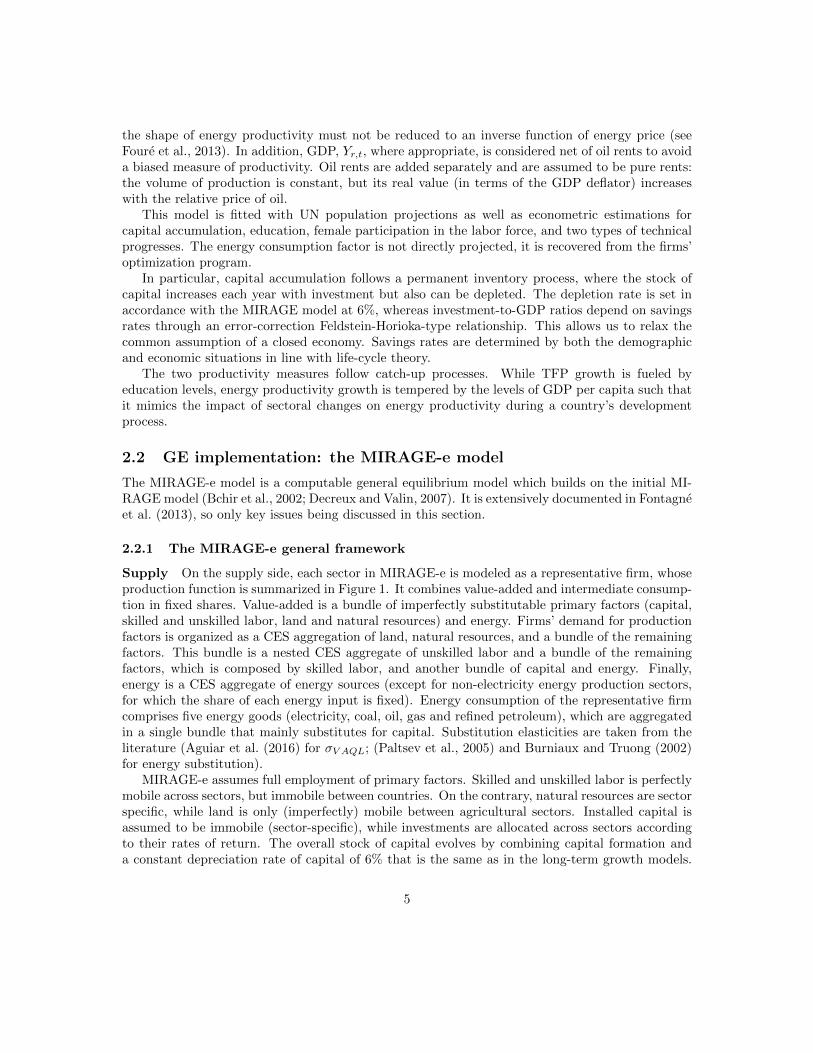
Supply On the supply side, each sector in MIRAGE-e is modeled as a representative firm, whoseproduction function is summarized in Figure 1. It combines value-added and intermediate consump-tion in fixed shares. Value-added is a bundle of imperfectly substitutable primary factors (capital,skilled and unskilled labor, land and natural resources) and energy. Firms’ demand for productionfactors is organized as a CES aggregation of land, natural resources, and a bundle of the remainingfactors. This bundle is a nested CES aggregate of unskilled labor and a bundle of the remainingfactors, which is composed by skilled labor, and another bundle of capital and energy. Finally,energy is a CES aggregate of energy sources (except for non-electricity energy production sectors,for which the share of each energy input is fixed). Energy consumption of the representative firmcomprises five energy goods (electricity, coal, oil, gas and refined petroleum), which are aggregatedin a single bundle that mainly substitutes for capital. Substitution elasticities are taken from theliterature (Aguiar et al. (2016) for σV AQL; (Paltsev et al., 2005) and Burniaux and Truong (2002)for energy substitution).
MIRAGE-e assumes full employment of primary factors. Skilled and unskilled labor is perfectlymobile across sectors, but immobile between countries. On the contrary, natural resources are sectorspecific, while land is only (imperfectly) mobile between agricultural sectors. Installed capital isassumed to be immobile (sector-specific), while investments are allocated across sectors accordingto their rates of return. The overall stock of capital evolves by combining capital formation anda constant depreciation rate of capital of 6% that is the same as in the long-term growth models.
5
Figure 1: Production function of firms in MIRAGE-e
Production of good i in region r
Intermediate Consumption Value Added and Energy
Leontief
Good 1 ... Good J
σIC=0.6
Land Natural Resources VAQL bundle
σVA
Unskilled Labor
σVAQL
Q bundle
Skilled Labor
σQ=0.6
KE bundle
KE Bundle
Capital Electricity Coal Other
σKE=0.5
Oil
σNCFF=1.01
Gas Refined oil
Gross investment is determined by the combination of saving and the current account. Finally, whiletotal investment is saving-driven, its allocation is determined by the rate of return on investment inthe various activities. For simplicity, and because we lack reliable data on foreign direct investmentat country of origin, host and sectoral levels, international capital flows only appear through thecurrent account imbalances, and have not been explicitly modeled yet.
Consumers On the demand side, a representative consumer from each country/region maximizesinstantaneous utility under a budget constraint, her savings being determined by saving ratesprojected in our first-step exercise. Expenditure is allocated to commodities and services accordingto a LES-CES (Linear Expenditure System – Constant Elasticity of Substitution) function. Thisimplies that, above a minimum consumption of goods produced by each sector, consumption choicesamong goods produced by different sectors are made according to a CES. This representation ofpreferences is well suited to our purpose as it is flexible enough to deal with countries at differentlevels of development. Elasticities and minimal consumption levels are calibrated such that theutility function reproduces at best price and income elasticities from USDA (USDA, 2005).
Trade Within each sector, total demand for each good (final, intermediate and investment) isdifferentiated by its origin. A nested CES function allows for a particular status for domesticproducts according to the usual Armington hypothesis (Armington, 1969), as depicted in Figure 2:consumers’ and firms’ choices are biased towards domestic production, and therefore domestic andforeign goods are imperfectly substitutable, using a CES specification. We use Armington elasticitiesprovided by the GTAP database (Global Trade Analysis Project) and estimated by Hertel et al.(2007) for σIMP and a simple rule of the thumb to relate to the (lower) σARM .
Issues with energy and CO2 emission accounting Using CES functional forms with vari-ables in monetary units leads to inconsistencies when trying to retrieve physical quantities. In ourcase, this matters for energy consumption, production, and trade, and their consequences for CO2
6
Figure 2: Demand in MIRAGE-e
Total demand for good i in region s
Domestic demand Import demand
σARM
Import from country 1 ... Import from country R
σIMP
emissions.3 Therefore, in addition to accounting relations in constant dollars, MIRAGE-e integratesa parallel accounting in energy physical quantities (in million tons of oil equivalent, Mtoe) allow-ing CO2 emissions to be computed (in million tons of carbon dioxide, MtCO2). Since the CESarchitecture does not maintain coherence in physical quantities, MIRAGE-e introduces energy- andcountry-specific adjustment coefficients. These two aggregation coefficients allow our basic energyaccounting relationships to remain valid. This means that the quantity produced by one country4,EYe,r,t must equal the demand in this country both local, EDe,r,t and from abroad, EDEMe,r,s,t,as in Equation (2) ; and energy consumption (by households, ECe,s,t and firms, EEICe,j,s,t) in onecountry must equal its local and foreign demand (Equation (3)).
EYe,r,t = EDe,r,t +∑s
EDEMe,r,s,t (2)
ECe,s,t +∑j
EEICe,j,s,t = EDe,s,t +∑r
EDEMe,r,s,t (3)
The corresponding adjustment coefficient, AgDeme,r,t (resp. AgConse,r,t) is re-scaling thecountry’s demand (resp. consumption) such that it matches the physical quantities produced (resp.demanded). In turn, only energy quantity produced is proportional to the volume production Y dueto its being above rather than inside the CES. Finally, CO2 emissions are recovered as proportionalto the energy quantities consumed, using energy-, sector- and country-specific factors determinedby the data.
Data sources MIRAGE-e mainly relies on the GTAP 9 database (Aguiar et al., 2016). However,along with this base data, the model relies on the HS6 level MAcMap database (Guimbard et al.,2012; Bouet et al., 2008) for tariff data and Minor (2013) (based on the methodology by Hummelsand Schaur, 2013) for trade costs associated with delays – modelled by and iceberg trade cost.
2.2.2 Consistent baseline implementation
Factor accumulation Availability of primary factors is determined by macroeconomic projec-tions.
3Preliminary simulations of MIRAGE-e showed that there could be a gap of more than 20% between a country’senergy consumption and energy demanded if proportionality was assumed between monetary and physical values.
4In these equations, and in the rest of this paper, the subscript e will be an index for energy goods. In addition,r denotes (where appropriate), the country of origin of a good and s denotes its destination.
7
• Skilled and unskilled labor grow at exogenous rates, taken from MaGE’s projections.
• Capital supply depends on two outputs from macro projections: the savings rate and thecurrent account balances, both of them varying exogenously.
• Natural resources for the mining sector and land for agricultural sectors are set at their 2004levels: prices adjust demand to this fixed supply.
• Natural resources for fossil fuel production sectors (coal, oil and gas) adjust to match theexogenous price target we impose (International Energy Agency, 2015) according to the energydemand projected by the model.
• Land (for agricultural sectors) expands following an iso-elastic function of real return to Land.
Dynamics in MIRAGE-e is sequentially recursive: the equilibrium is solved successively for eachperiod by adjusting to projected growth in the variables described above. The time span of thislong-run baseline is 2011-2100. Over this time period, capital stocks change according to investmentdecisions based on rates of return to capital at sectoral level and the depreciation rate, which isassumed to be constant and uniform across regions (i.e. δ = 6%).
Kj,r,s,t = Kj,r,s,t−1.(1 − δ) + INVj,r,s,t (4)
Factor productivity Only three production factors, namely the two forms of labour and capital,are subject to productivity improvement. The level of productivity is also mainly derived frommacroeconomic projections in the baseline, but some sector variations are taken into account.Indeed, factor productivity improvements follow the following rules: (i) at the regional level, theaverage productivity must make GDP growth match the level of the macroeconomic projections ;(ii) agricultural productivity is exogenous, coming from a Data Envelopment Analysis documentedin Fontagne et al. (2013) ; and (iii) we follow the methodology by Van der Mensbrugghe (2010),using estimates from Bernard and Jones (1996) and Timmer et al. (2010), by imposing that theproductivity in manufacturing is 2 p.p. greater than for services.
Energy productivity Contrary to other components that act as production factors, energyuse is subject to its own technological improvements. Energy productivity follows the trajectorycoming from the macroeconomic projections. The only exception concerns non-electricity energyproduction sectors (coal, oil, gas and refined petroleum), in order to avoid creating energy out ofnowhere and in line with our “constant energy production technology” assumption.
Macroeconomic closure Finally, the macroeconomic closure of the model is achieved throughthe imposition of an exogenous current account imbalance. We believe that this imbalance is mainlydriven by demographics, through its impact on the savings and investment, and thus the variation incurrent account follows the variation in the macroeconomic projections (measured as a percentageof world GDP in order to maintain consistency between each regional imbalance). With such amacroeconomic closure, trade imbalances are then exogenous, and the (implicit) real exchange rateadjusts.
8
Figure 3: Complete articulation of the models and assumptions
Assumptions on :PopulationEducationInstitutionsTFP frontier
Energy productivityOil price
Assumptions on :Coal and gas prices
Assumptions on :Trade policy
Policy experiment :Climate mitigation
2.2.3 Summary of quantification strategy
As a result from our modelling framework, we propose the workflow depicted in Figure 3 to quantifyat best any policy in the context of uncertain global conjuncture. This strategy consists in foursteps, illustrated in the Figure by the exercise described later in this chapter.
1. Macroeconomic projections: The variables of interest (GDP, population, etc.) are projectedwith the macroeconomic model.
2. Baseline Step 1: This global projection is broken down at the sectoral level by the CGEmodel, with as few additional assumptions as possible.
3. Baseline Step 2: Baseline assumptions that go beyond macroeconomics (i.e. sector-specificassumptions that have an impact on GDP growth) are implemented in the CGE model.
4. Simulation: The actual policy experiment to be evaluated is implemented and compared toBaseline Step 2.
3 An application to the quantification of Shared Socio-economicPathways
Building on an initiative by the Intergovernmental Panel on Climate Change (IPCC), researchersof the climate change field have been conducting since 2010 an interdisciplinary exercise in orderto identify the key elements that would impact the potential magnitude and cost of climate changemitigation over the 21st century. The outcome of these working groups has been the elaboration of
9
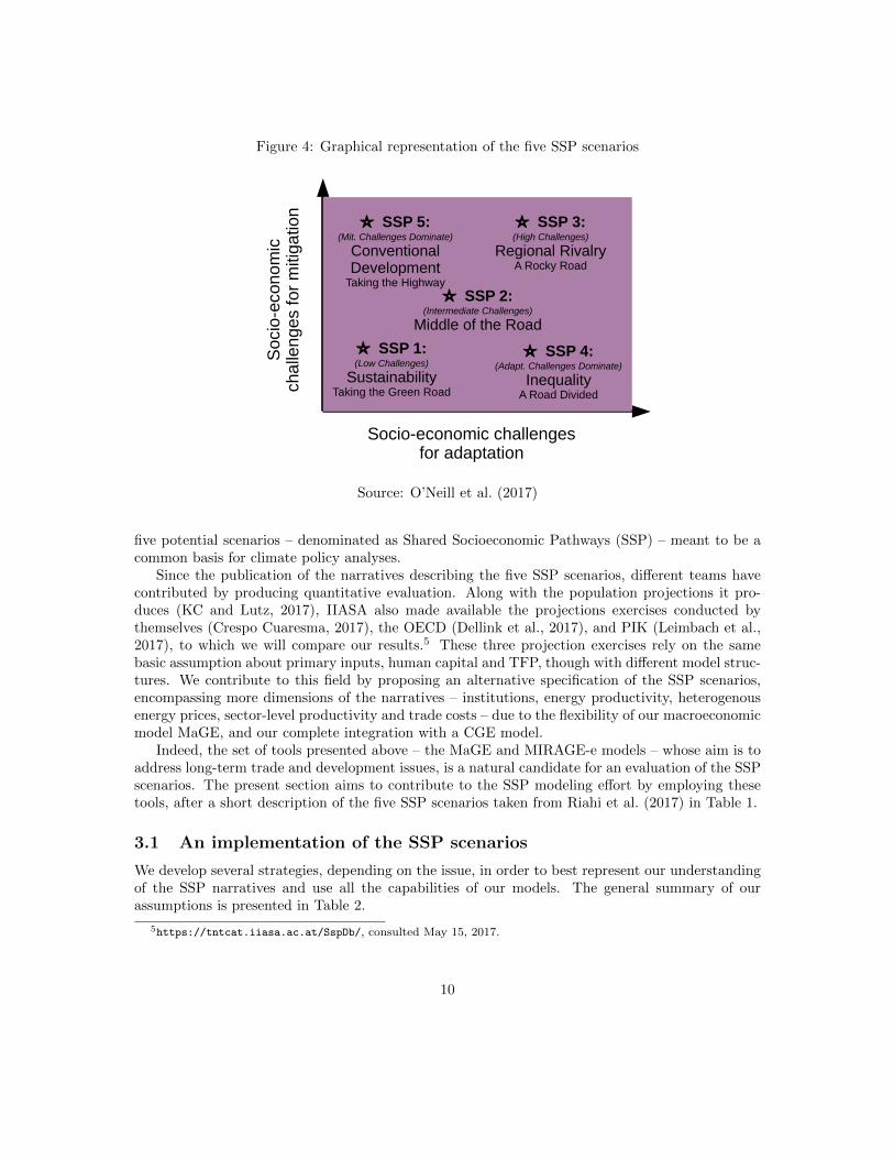
Figure 4: Graphical representation of the five SSP scenarios
So
cio
-eco
nom
icch
alle
ng
es fo
r m
itiga
tion
Socio-economic challengesfor adaptation
SSP 5:(Mit. Challenges Dominate)
ConventionalDevelopment
Taking the Highway
SSP 3:(High Challenges)
Regional RivalryA Rocky Road
SSP 2:(Intermediate Challenges)
Middle of the Road
SSP 1:(Low Challenges)
SustainabilityTaking the Green Road
SSP 4:(Adapt. Challenges Dominate)
InequalityA Road Divided
Source: O’Neill et al. (2017)
five potential scenarios – denominated as Shared Socioeconomic Pathways (SSP) – meant to be acommon basis for climate policy analyses.
Since the publication of the narratives describing the five SSP scenarios, different teams havecontributed by producing quantitative evaluation. Along with the population projections it pro-duces (KC and Lutz, 2017), IIASA also made available the projections exercises conducted bythemselves (Crespo Cuaresma, 2017), the OECD (Dellink et al., 2017), and PIK (Leimbach et al.,2017), to which we will compare our results.5 These three projection exercises rely on the samebasic assumption about primary inputs, human capital and TFP, though with different model struc-tures. We contribute to this field by proposing an alternative specification of the SSP scenarios,encompassing more dimensions of the narratives – institutions, energy productivity, heterogenousenergy prices, sector-level productivity and trade costs – due to the flexibility of our macroeconomicmodel MaGE, and our complete integration with a CGE model.
Indeed, the set of tools presented above – the MaGE and MIRAGE-e models – whose aim is toaddress long-term trade and development issues, is a natural candidate for an evaluation of the SSPscenarios. The present section aims to contribute to the SSP modeling effort by employing thesetools, after a short description of the five SSP scenarios taken from Riahi et al. (2017) in Table 1.
3.1 An implementation of the SSP scenarios
We develop several strategies, depending on the issue, in order to best represent our understandingof the SSP narratives and use all the capabilities of our models. The general summary of ourassumptions is presented in Table 2.
5https://tntcat.iiasa.ac.at/SspDb/, consulted May 15, 2017.
SSP1 Systainability – Taking the Green RoadThe world shifts gradually, but pervasively, toward a more sustainable path, emphasizing more inclusivedevelopment that respects perceived environmental boundaries. Management of the global commons slowlyimproves, educational and health investments accelerate the demographic transition, and the emphasis oneconomic growth shifts toward a broader emphasis on human well-being. Driven by an increasing commit-ment to achieving development goals, inequality is reduced both across and within countries. Consumptionis oriented toward low material growth and lower resource and energy intensity.
SSP2 Middle of the RoadThe world follows a path in which social, economic, and technological trends do not shift markedly from his-torical patterns. Development and income growth proceeds unevenly, with some countries making relativelygood progress while others fall short of expectations. Global and national institutions work toward but makeslow progress in achieving sustainable development goals. Environmental systems experience degradation,although there are some improvements and overall the intensity of resource and energy use declines. Globalpopulation growth is moderate and levels off in the second half of the century. Income inequality persists orimproves only slowly and challenges to reducing vulnerability to societal and environmental changes remain.
SSP3 Regional Rivalry – A Rocky RoadA resurgent nationalism, concerns about competitiveness and security, and regional conflicts push countriesto increasingly focus on domestic or, at most, regional issues. Policies shift over time to become increasinglyoriented toward national and regional security issues. Countries focus on achieving energy and food securitygoals within their own regions at the expense of broader-based development. Investments in education andtechnological development decline. Economic development is slow, consumption is material-intensive, andinequalities persist or worsen over time. Population growth is low in industrialized and high in developingcountries. A low international priority for addressing environmental concerns leads to strong environmentaldegradation in some regions.
SSP4 Inequality – A Road DividedHighly unequal investments in human capital, combined with increasing disparities in economic opportu-nity and political power, lead to increasing inequalities and stratification both across and within countries.Over time, a gap widens between an internationally-connected society that contributes to knowledge- andcapital-intensive sectors of the global economy, and a fragmented collection of lower-income, poorly educatedsocieties that work in a labor intensive, low-tech economy. Social cohesion degrades and conflict and unrestbecome increasingly common. Technology development is high in the high-tech economy and sectors. Theglobally connected energy sector diversifies, with investments in both carbon-intensive fuels like coal andunconventional oil, but also low-carbon energy sources. Environmental policies focus on local issues aroundmiddle and high income areas.
SSP5 Conventional Development – Taking the HighwayThis world places increasing faith in competitive markets, innovation and participatory societies to pro-duce rapid technological progress and development of human capital as the path to sustainable development.Global markets are increasingly integrated. There are also strong investments in health, education, andinstitutions to enhance human and social capital. At the same time, the push for economic and socialdevelopment is coupled with the exploitation of abundant fossil fuel resources and the adoption of resourceand energy intensive lifestyles around the world. All these factors lead to rapid growth of the global econ-omy, while global population peaks and declines in the 21st century. Local environmental problems like airpollution are successfully managed. There is faith in the ability to effectively manage social and ecologicalsystems, including by geo-engineering if necessary.
Source: Riahi et al. (2017)
11
Demographics and education Our approach regarding demographics is hybrid, since all thedimensions cannot be directly encompassed using MaGE. Furthermore, other institutions havepublished detailed demographic scenarios, in particular the IIASA (KC and Lutz, 2017). TheseIIASA scenarios already include variation in mortality, fertility and migration, whereas MaGEcan only deal with some migrations flows. We therefore chose to rely on IIASA projections forpopulation.
Regarding education, two options were available: use IIASA projections or develop scenariosdirectly in MaGE. On the one hand, MaGE projections would have been more flexible, but on theother hand, IIASA include the impact of education on fertility. We then chose IIASA projectionsto keep a maximum consistency.
Finally, total population has to be converted into active population. On this matter, MaGEprovides the best framework by including variation in female participation to the labor force dueto increases in education level.
Institutions The economic literature has studied institutions and their impact for long. Forinstance, Aron (2000) documents that institutions interfere in the accumulation of all productionfactors, and in particular by productivity improvements – both regarding innovation and catch-upto the technological frontier – and in capital accumulation. Quite often, as the author suggests,institutions are limited to productivity improvements, neglecting all other aspects. We will try todepart from this common assumption.
Although not explicitly specified, institutions differentials appear in MaGE in two ways. Firstof all, they are embodied in the fixed effects that are estimated in our econometric relationships(TFP, savings rate, female participation to the labor force and savings-investment relation). Sec-ond, institutions also appear in the Feldstein-Horioka relation, because we conduct two separateestimations on two different country groups (OECD countries vs. non-OECD countries). As a con-sequence, the estimated coefficients embody institutional differences between OECD members andother countries. Scenarios of institutional convergence can then be derived from these two ways.
However, quantifying the magnitude of the impact of institutions on our variables of interest issubject to judgment: to our knowledge the literature has not investigated the quantitative impactof institutions on other variables than TFP. Therefore, productivity improvements due to improve-ments in institutions efficiency will be derived from estimates from the literature – as describedbelow – while we will have a simple normative definition of efficient institutions regarding othervariables (savings rate, female participation and savings-investment relationship).
The link between productivity improvements and institutional environment has been quanti-fied by Chanda and Dalgaard (2008). The impact of institutions – measured by the GovernmentAnti-Diversionary Policy (GADP) index – on the level of TFP is tackled using several estimationstrategies (Ordinary Least Squares – OLS – and 2-Stage Least Squares – 2SLS – with instrumentalvariables). Endogeneity issues were finally not convincingly addressed and the results provide onlyorders of magnitude of the actual impact of institutions on TFP. We convert these results into arange of potential TFP variations – from -30% to +50% – which corresponds to a one-standard-errorchange in the GADP index.
Regarding other relations that are impacted by institutional convergence, we will arbitrarilyconsider then institutions in OECD countries are more efficient than in non-OECD countries, andas a consequence, convergence towards more efficient institutions will only impact non-OECD coun-tries, making them converge by 2100 to the average OECD institutions (both the fixed effects andother estimated coefficients converge).
12
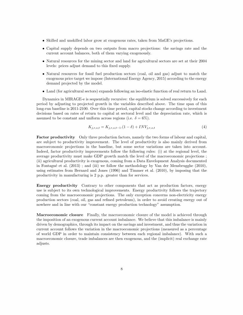
Technology First of all, SSP narratives include scenarios on the technological frontier. This TFPfrontier is present in MaGE, and is represented by the TFP level of Ireland and Denmark (these twocountries share the leadership over our estimation period). Other countries converge towards thetechnological frontier conditionally on their education level. In projection, the baseline assumptionin MaGE is that the TFP frontier continues to grow at its 1995-2008 average pace (around 1.5%annual growth). The amount of additional TFP for leader countries in SSP scenarios is howevernot easily determined, so we will consider scenarios where the TFP leader level of TFP growthis +/-50% of the baseline growth rate. The second issue about technology scenarios is energyproductivity. We will consider a 50% increase in energy productivity by 2100, or alternatively onlya 25% decrease in order to avoid theoretical infeasibility in the growth model when energy pricesbecome greater than energy productivity.
Fossil constraints Fossil constraints in MaGE are materialized by oil price, whose trajectorybinds the amount of energy use given the current level of energy-specific productivity. In MIRAGE,we can further differentiate the type of energy, and consider different prices for coal, oil and gas.The central scenario in both models corresponds to the medium projections of the InternationalEnergy Agency (IEA), taken from the World Energy Outlook (International Energy Agency, 2015).Accordingly, high and low fossil resource prices scenarios will be derived from their counterparts inIEA projections (resp. “current policies” and ”low oil price” scenarios).
Figure 5: Energy prices, 2011=1, 2011-2100
1
2
3
4
5
2025 2050 2075 2100Time
Wor
ld a
vera
ge p
rice
(201
1=1)
Primary energy
Coal
Gas
Oil
Scenario
High (SSP4)
Low (SSP5)
Medium
Source: International Energy Agency (2015) and authors’ computations.Vertical line denotes the transition between IEA projections and simple extrapolation.
Sector structure and international trade MaGE does not encompass the sector structureof the economy, but MIRAGE does. The shift in structure (final and intermediate demand) isdriven by relative prices and productivity differential. In our central case, agricultural productivityis exogenous (following the projections documented in Fontagne et al. (2013) while we constrainservices productivity growth to be 2 percentage points lower than industrial TFP. The nationalaverage TFP level is computed given these constraints, plus the need to match MaGE projectionsin terms of GDP. Accordingly, our scenarios build on this productivity structure.
13
The choice to implement sector-level scenarios in Step 1 or Step 2 does matter a lot for the re-sults, in particular when dealing with productivity improvement.6 However, in the SSP narratives,it is not always obvious whether a technological development is more about additional innovation(then, the sectoral scenario goes in Step 2) or about the allocation of innovation (then, it shouldbe implemented in Step 1). In order to choose between the two alternative, we took particular at-tention to wording in the narratives. On agriculture, O’Neill et al. (2017) mentions “improvementsin technology” (SSP1) and “rapid increase in productivity” (SSP5), hence suggesting that tech-nological improvements come in addition to other assumptions. On the contrary, regarding fossilfuel productivity, one read ”preferences shift away from fossil fuels” (SSP1), suggesting that it ismore a matter of allocation than technological improvements. Finally, on services, the paper reads“the service sector grows relatively quickly” (SSP1), but at the same time the emphasis is on “lowgrowth in material consumption”. We therefore retain an implementation in Step 1 (technology isbiased towards services).
As for scenarios, a more (resp. less) productive agriculture will correspond to a 0.2% additional(resp. less) annual productivity growth, corresponding roughly to the average productivity growthin crops sector. In addition, productivity growth in services will be 1 p.p. greater when necessary(the gap between manufacturing and services is narrowed by half). The same magnitude (+/-1 p.p.growth) is retained for the fossil fuel production sectors.
Finally, international trade is influenced by tariffs and other transaction costs faced by exporters,as well as by energy prices through transport, as documented in Fontagne and Foure (2013). Wefocus on the two first determinants, since energy prices scenarios are derived separately, taking theassumptions elaborated in Fontagne and Foure (2013). Namely, we consider (i) a world trade war by2100 resulting in a return to post-Kennedy round tariffs (in 1967)7 ; or (ii) a global liberalizationresulting in a 50% decrease in tariffs plus 20% decrease in transaction costs. Both assumptionsnaturally happen in Step 2, because they are likely to influence GDP growth by a channel notpresent in Step 1.
Summary Table 3 summarizes the assumptions made to represent at best the five SSP narrativescenarios.
6For instance, simulations not present in this paper showed that implementing services productivity improvementin Step 2 instead of Step 1 could reverse the ordering of SSP 1 and SSP 5 scenarios in terms of world GDP.
7When available, we retain tariffs from Deardorff and Stern (1983), and otherwise we use simple order of magni-tudes assuming the reversal of previous changes. An increase by 24% in primary sectors’ tariffs is assumed, as wellas an increase by 25% in manufacturing plus an increase in transaction costs by 20%
14
Table 2: MaGE-MIRAGE implementation of the SSP scenarios
SSP1 SSP2 SSP3 SSP4 SSP5 ModelTopic Sustainability Middle of the road Fragmentation Inequality Conventional concerned
Population Provided by IIASA MaGEEducation Provided by IIASA MaGEInstitutions Convergenc of fixed
effects– -30% TFP OECD:+50% TFP
; Other: -30%+50% TFP ; con-vergence of fixed ef-fects
3.2 Illustration with a simple climate change mitigation policy
3.2.1 Data and aggregation
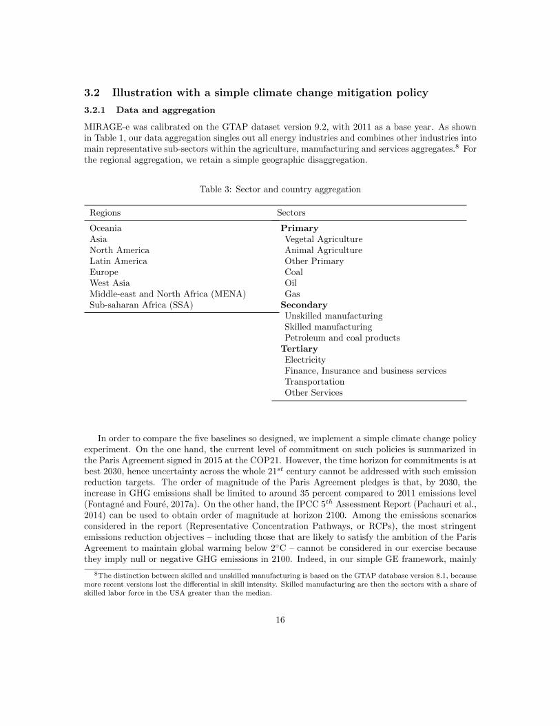
MIRAGE-e was calibrated on the GTAP dataset version 9.2, with 2011 as a base year. As shownin Table 1, our data aggregation singles out all energy industries and combines other industries intomain representative sub-sectors within the agriculture, manufacturing and services aggregates.8 Forthe regional aggregation, we retain a simple geographic disaggregation.
Table 3: Sector and country aggregation
Regions
OceaniaAsiaNorth AmericaLatin AmericaEuropeWest AsiaMiddle-east and North Africa (MENA)Sub-saharan Africa (SSA)
SecondaryUnskilled manufacturingSkilled manufacturingPetroleum and coal products
TertiaryElectricityFinance, Insurance and business servicesTransportationOther Services
In order to compare the five baselines so designed, we implement a simple climate change policyexperiment. On the one hand, the current level of commitment on such policies is summarized inthe Paris Agreement signed in 2015 at the COP21. However, the time horizon for commitments is atbest 2030, hence uncertainty across the whole 21st century cannot be addressed with such emissionreduction targets. The order of magnitude of the Paris Agreement pledges is that, by 2030, theincrease in GHG emissions shall be limited to around 35 percent compared to 2011 emissions level(Fontagne and Foure, 2017a). On the other hand, the IPCC 5th Assessment Report (Pachauri et al.,2014) can be used to obtain order of magnitude at horizon 2100. Among the emissions scenariosconsidered in the report (Representative Concentration Pathways, or RCPs), the most stringentemissions reduction objectives – including those that are likely to satisfy the ambition of the ParisAgreement to maintain global warming below 2◦C – cannot be considered in our exercise becausethey imply null or negative GHG emissions in 2100. Indeed, in our simple GE framework, mainly
8The distinction between skilled and unskilled manufacturing is based on the GTAP database version 8.1, becausemore recent versions lost the differential in skill intensity. Skilled manufacturing are then the sectors with a share ofskilled labor force in the USA greater than the median.
16
constituted by CES functional forms, this would imply negative or null economic activity due tothe lack of technological breakthrough or carbon sinks. We therefore concentrate on less ambitiousscenarios, namely RCP6.0, that are only “likely” to limit global warming by 4◦C. These RCP6.0scenarios result on average in a limitation of global GHG emissions to an increase by around 30%in 2100 compared to 2011.
In our simulations, we implement a global carbon market with the objective to limit the increasein CO2 emissions to 30% by 2100 – or, put differently, make the assumption that the world willimplement a carbon tax high enough to achieve this goal.
3.2.2 The five SSP baselines
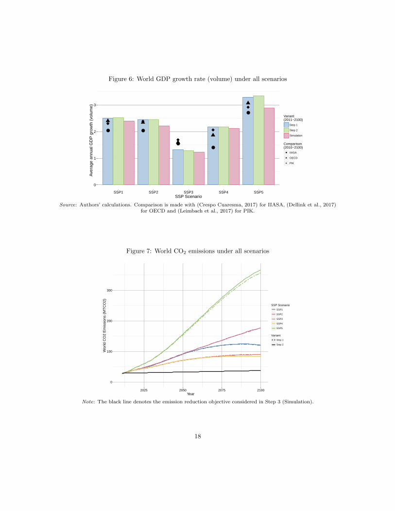
Baseline economic growth Figure 6 shows our results on average GDP growth (2011-2100) inall scenarios, but for the moment we will focus on the baseline steps 1 and 2 (resp. blue and greenbars).
Our projected GDP growth rates range from 1.3 to 3.3 % at the world level, ranking SSP sce-narios in a consistent way, from SSP3 being the less economically favourable case to a very dynamicworld economy in SSP5. In addition, our results show that very contrasted trade policy scenariosin SSP 3 and 5 (respectively a return to post-Tokyo round tariffs and a full tariff liberalization withNTM reductions) only lead to sizeable but moderate differences in overall economic activity. Thisconclusion is consistent with the trade policy analysis literature, where trade liberalization onlylead to slight increases in GDP.
Regarding the way we compare alternative SSP evaluations (Crespo Cuaresma, 2017; Dellinket al., 2017; Leimbach et al., 2017), two issues are worth mentioning. First, from a methodologicalpoint of view, other SSP evaluations are only comparable to our Step 1 (i.e. without trade policy).On this regard, our estimations are in the same order of magnitude, but more contrasted, especiallyregarding SSP3 and SSP5. This difference is not that surprising, as the three cited modellingteams have harmonized their interpretation of the SSP storylines, and therefore present the samescenarios with only a difference in the underlying models. On the contrary, we built an independentinterpretation of the SSP storylines consistent with our model. By doing so, we ended up withspecific quantification of TFP shocks – the most important driver of baseline growth – based oneconometric estimations, and even go beyond TFP scenarios by including other determinants inboth the macroeconomic growth model and the CGE.
Second, the introduction of a second SSP baseline step (including trade policies) further widenthe contrast between our projected baseline GDP growth and other projections, though the differ-ence is of second order.
CO2 emissions On CO2 emissions, our results are even more contrasted, ranging from an 190(SSP 4) to 1100 % (SSP 5) increase in emissions level. However, this quantification may not beconsidered more than a simple illustration of potential applications for our SSP baselines. Indeed,the MIRAGE-e model is not well fitted to deal with such long-run emissions: renewable energiesare not explicit, hence constrained at their 2011 share ; emission factors for fossil fuels are constant; and no carbon sink is considered either. As a result, if we compare to alternative quantifications,e.g. from (Pachauri et al., 2014), our figures are much higher.
However, these emissions results are worth considering, as Figure 7 show that only a veryambitious trade liberalization in SSP5 could have a sizeable impact on global emissions, boththrough increased economic activity and increased demand for international transportation.
17
Figure 6: World GDP growth rate (volume) under all scenarios
● ●
●●
●
0
1
2
3
SSP1 SSP2 SSP3 SSP4 SSP5SSP Scenario
Ave
rage
ann
ual G
DP
gro
wth
(vo
lum
e)
Variant (2011−2100)
Step 1
Step 2
Simulation
Comparison (2010−2100)
● IIASA
OECD
PIK
Source: Authors’ calculations. Comparison is made with (Crespo Cuaresma, 2017) for IIASA, (Dellink et al., 2017)for OECD and (Leimbach et al., 2017) for PIK.
Figure 7: World CO2 emissions under all scenarios
0
100
200
300
2025 2050 2075 2100Year
Wor
ld C
O2
Em
issi
ons
(MT
CO
2)
SSP Scenario
SSP1
SSP2
SSP3
SSP4
SSP5
Variant
Step 1
Step 2
Note: The black line denotes the emission reduction objective considered in Step 3 (Simulation).
18
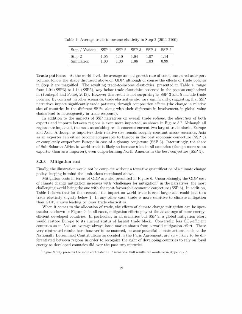
Table 4: Average trade to income elasticity in Step 2 (2011-2100)
Trade patterns At the world level, the average annual growth rate of trade, measured as exportvolume, follow the shape discussed above on GDP, although of course the effects of trade policiesin Step 2 are magnified. The resulting trade-to-income elasticities, presented in Table 4, rangefrom 1.04 (SSP3) to 1.14 (SSP5), way below trade elasticities observed in the past as emphasizedin (Fontagne and Foure, 2013). However this result is not surprising as SSP 3 and 5 include tradepolicies. By contrast, in other scenarios, trade elasticities also vary significantly, suggesting that SSPnarratives impact significantly trade patterns, through composition effects (the change in relativesize of countries in the different SSPs, along with their difference in involvement in global valuechains lead to heterogeneity in trade response).
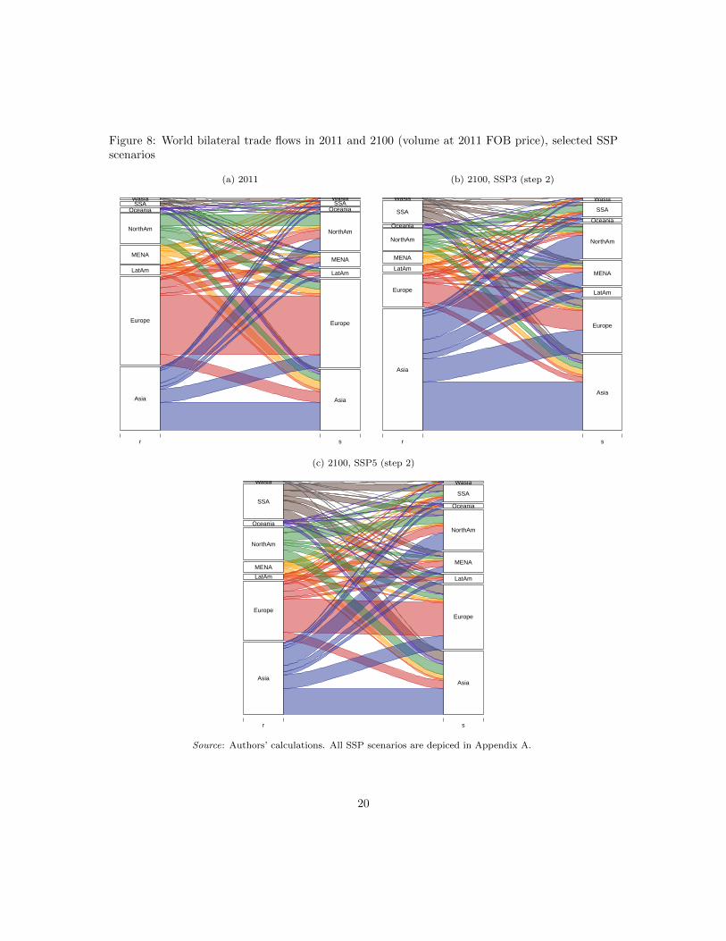
In addition to the impacts of SSP narratives on overall trade volume, the allocation of bothexports and imports between regions is even more impacted, as shown in Figure 8.9 Although allregions are impacted, the most astonishing result concerns current two largest trade blocks, Europeand Asia. Although as importers their relative size remain roughly constant across scenarios, Asiaas an exporter can either become comparable to Europe in the best economic conjecture (SSP 5)or completely outperform Europe in case of a gloomy conjecture (SSP 3). Interestingly, the shareof Sub-Saharan Africa in world trade is likely to increase a lot in all scenarios (though more as anexporter than as a importer), even outperforming North America in the best conjecture (SSP 5).
3.2.3 Mitigation cost
Finally, the illustration would not be complete without a tentative quantification of a climate changepolicy, keeping in mind the limitations mentioned above.
Mitigation costs in terms of GDP are also presented in Figure 6. Unsurprisingly, the GDP costof climate change mitigation increases with “challenges for mitigation” in the narratives, the mostchallenging world being the one with the most favourable economic conjecture (SSP 5). In addition,Table 4 shows that for this scenario, the impact on world trade is even larger and could lead to atrade elasticity slightly below 1. In any other case, trade is more sensitive to climate mitigationthan GDP, always leading to lower trade elasticities.
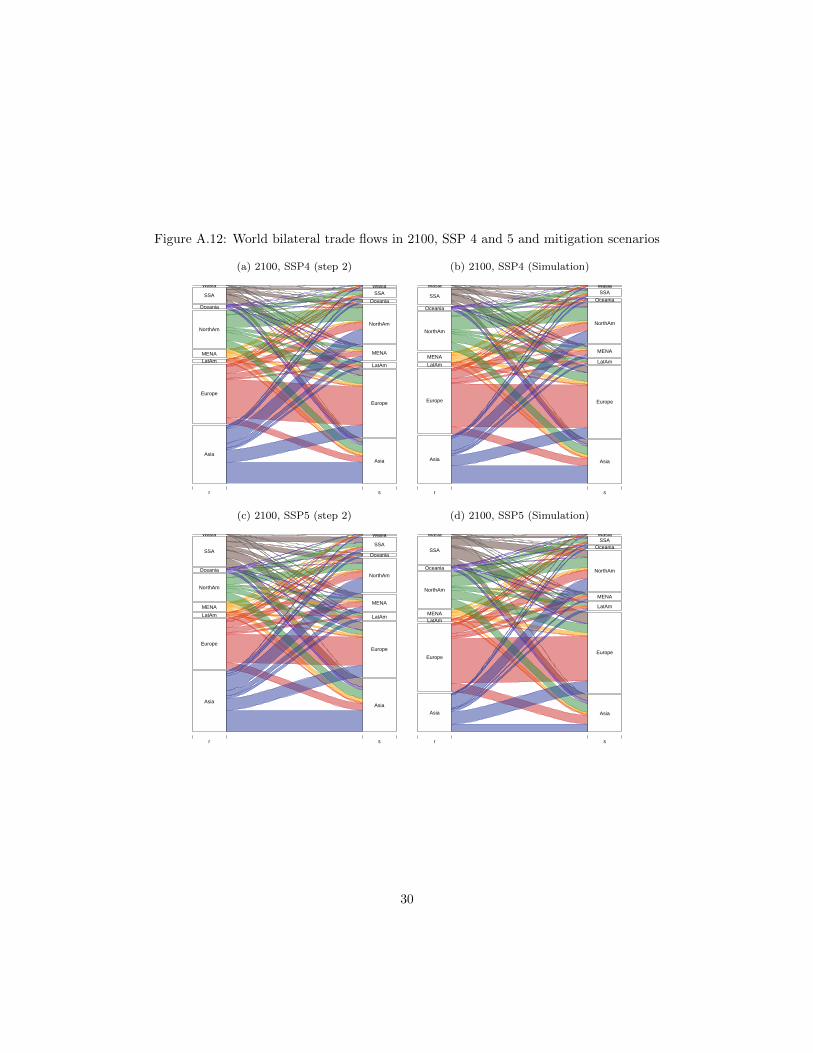
When it comes to the allocation of trade, the effects of climate change mitigation can be spec-tacular as shown in Figure 9: in all cases, mitigation efforts play at the advantage of more energy-efficient developed countries. In particular, in all scenarios but SSP 3, a global mitigation effortwould restore Europe to its current status of largest trade block. Conversely, less CO2-efficientcountries as in Asia on average always loose market shares from a world mitigation effort. Thesevery contrasted results have however to be nuanced, because potential climate actions, such as theNationally Determined Contributions as decided in the Paris Agreement, are very likely to be dif-ferentiated between regions in order to recognize the right of developing countries to rely on fossilenergy as developed countries did over the past two centuries.
9Figure 8 only presents the more contrasted SSP scenarios. Full results are available in Appendix A
19
Figure 8: World bilateral trade flows in 2011 and 2100 (volume at 2011 FOB price), selected SSPscenarios
(a) 2011
Asia
Europe
LatAm
MENA
NorthAm
OceaniaSSA
Wasia
Asia
Europe
LatAm
MENA
NorthAm
OceaniaSSA
Wasia
r s
(b) 2100, SSP3 (step 2)
Asia
Europe
LatAm
MENA
NorthAm
Oceania
SSA
Wasia
Asia
Europe
LatAm
MENA
NorthAm
Oceania
SSA
Wasia
r s
(c) 2100, SSP5 (step 2)
Asia
Europe
LatAm
MENA
NorthAm
Oceania
SSA
Wasia
Asia
Europe
LatAm
MENA
NorthAm
Oceania
SSA
Wasia
r s
Source: Authors’ calculations. All SSP scenarios are depiced in Appendix A.
20
Figure 9: World bilateral trade flows in 2100 with and without climage change mitigation, selectedSSP scenarios
(a) SSP2 – Step 2
Asia
Europe
LatAm
MENA
NorthAm
Oceania
SSA
Wasia
Asia
Europe
LatAm
MENA
NorthAm
Oceania
SSA
Wasia
r s
(b) SSP2 – Simulation
Asia
Europe
LatAmMENA
NorthAm
Oceania
SSA
Wasia
Asia
Europe
LatAm
MENA
NorthAm
OceaniaSSA
Wasia
r s
(c) SSP5 – Step 2
Asia
Europe
LatAm
MENA
NorthAm
Oceania
SSA
Wasia
Asia
Europe
LatAm
MENA
NorthAm
Oceania
SSA
Wasia
r s
(d) SSP5 - Simulation
Asia
Europe
LatAmMENA
NorthAm
Oceania
SSA
Wasia
Asia
Europe
LatAm
MENA
NorthAm
OceaniaSSA
Wasia
r s
21
4 Concluding remarks
We proposed in this chapter a sound, theoretically founded baseline of the world economy con-sistent with the SSP baseline methodology, along with an quantitative illustration. Although thequantification is not of paramount importance per se, due to model limitations, several mechanismsdrawn from our results are informative for future modelling works. First, trade policies play only alimited role in both trade patterns and mitigation costs as compared to underlying macroeconomiclong term determinants: trade patterns are way more impacted by macroeconomic determinants ofgrowth and climate change mitigation policies. These findings calls for a deepening of the kind ofapproaches presented here.
22
References
Aguiar, A., Narayanan, B., and McDougall, R. (2016). An overview of the GTAP 9 data base.Journal of Global Economic Analysis, 1(1):181–208.
Akgul, Z., Villoria, N. B., and Hertel, T. W. (2016). GTAP-HET: Introducing firm heterogeneityinto the GTAP model. Journal of Global Economic Analysis, 1(1):111–180.
Arkolakis, C., Costinot, A., and Rodrıguez-Clare, A. (2012). New trade models, same old gains?The American Economic Review, 102(1):94–130.
Armington, P. S. (1969). A theory of demand for products distinguished by place of production.Staff Papers - International Monetary Fund, 16(1):159.
Aron, J. (2000). Growth and institutions: A review of the evidence. The World Bank ResearchObserver, 15(1):99–135.
Bchir, H., Decreux, Y., Guerin, J.-L., and Jean, S. (2002). Mirage, a computable general equilibriummodel for trade policy analysis. Technical report, Unlisted. CEPII Working Paper.
Bernard, A. and Jones, C. (1996). Comparing apples to oranges: productivity convergence andmeasurement across industries and countries. The American Economic Review, 86(5):1216–1238.
Bouet, A., Decreux, Y., Fontagne, L., Jean, S., and Laborde, D. (2008). Assessing applied protectionacross the world. Review of International Economics, 16(5):850–863.
Burniaux, J. and Truong, T. (2002). Gtap-e: an energy-environmental version of the gtap model.GTAP Technical Papers, page 18.
Chanda, A. and Dalgaard, C.-J. (2008). Dual economies and international total factor produc-tivity differences: Channelling the impact from institutions, trade, and geography. Economica,75(300):629–661.
Crespo Cuaresma, J. (2017). Income projections for climate change research: A framework basedon human capital dynamics. Global Environmental Change, 42:226–236.
Deardorff, A. V. and Stern, R. M. (1983). Economic effects of the tokyo round. Southern EconomicJournal, 49(3):605.
Decreux, Y. and Valin, H. (2007). Mirage, updated version of the model for trade policy analysis:Focus on agriculture and dynamics. CEPII Working Papers.
Dellink, R., Chateau, J., Lanzi, E., and Magne, B. (2017). Long-term economic growth projectionsin the shared socioeconomic pathways. Global Environmental Change, 42:200–214.
Dixon, P. B. and Rimmer, M. T. (1998). Forecasting and Policy Analysis with a Dynamic CGEModel of Australia. Centre of Policy Studies/IMPACT Centre Working Papers op-90, VictoriaUniversity, Centre of Policy Studies/IMPACT Centre.
Duval, R. and de la Maisonneuve, C. (2010). Long-run growth scenarios for the world economy.Journal of Policy Modeling, 32(1):64–80.
23
Feenstra, R., Luck, P., Obstfeld, M., and Russ, K. (2014). In search of the armington elasticity.Technical report.
Fontagne, L. and Foure, J. (2013). Opening a pandora’s box: Modelling world trade patterns atthe2035 horizon. CEPII Working Paper, 2013-22.
Fontagne, L. and Foure, J. (2017a). La politique commerciale au service de la politique climatique.La Lettre du CEPII, 2017(373).
Fontagne, L. and Foure, J. (2017b). Value added in motion: Modelling world trade patterns at the2035 horizon. Technical report.
Fontagne, L., Foure, J., and Keck, A. (2017a). Simulating world trade in the decades ahead: drivingforces and policy implications. The World Economy, 40(1):36–55.
Fontagne, L., Foure, J., and Ramos, M. P. (2013). MIRAGE-e: A general equilibrium long-termpath of the world economy. CEPII Working Paper, 2013-39.
Fontagne, L., Martin, P., Orefice, G., et al. (2017b). The international elasticity puzzle is worsethan you think. Technical report, CEPR discussion paper 11855.
Foure, J., Benassy-Quere, A., and Fontagne, L. (2013). Modelling the world economy at the 2050horizon. Economics of Transition, pages 617–654.
Guimbard, H., Jean, S., Mimouni, M., and Pichot, X. (2012). Macmap-hs6 2007, an exhaustiveand consistent measure of applied protection in 2007. International Economics, 130:99–121.
Hertel, T., Hummels, D., Ivanic, M., and Keeney, R. (2007). How confident can we be of CGE-basedassessments of free trade agreements? Economic Modelling, 24(4):611–635.
Hogan, W. P. (1958). Technical progress and production functions. The Review of Economics andStatistics, 40(4):407.
Hummels, D. L. and Schaur, G. (2013). Time as a trade barrier. American Economic Review,103(7):2935–2959.
Ianchovichina, E., McDougall, R., and Hertel, T. (2000). A disequilibrium model of internationalcapital mobility.
International Energy Agency (2015). World Energy Outlook 2015. OECD Publishing.
KC, S. and Lutz, W. (2017). The human core of the shared socioeconomic pathways: Populationscenarios by age, sex and level of education for all countries to 2100. Global EnvironmentalChange, 42:181–192.
Leimbach, M., Kriegler, E., Roming, N., and Schwanitz, J. (2017). Future growth patterns of worldregions – a GDP scenario approach. Global Environmental Change, 42:215–225.
Lemelin, A. and Robichaud, V. (2015). Calibrating a reference scenario for a multi-region, recursivedynamic world cge model.
Lucas, R. E. (1988). On the mechanics of economic development. Journal of Monetary Economics,22(1):3–42.
24
Mankiw, N. G., Romer, D., and Weil, D. N. (1992). A contribution to the empirics of economicgrowth. The Quarterly Journal of Economics, 107(2):407–437.
Markandya, A. and Pedroso-Galinato, S. (2007). How substitutable is natural capital? Environ-mental and Resource Economics, 37(1):297–312.
Melitz, M. J. (2003). The impact of trade on intra-industry reallocations and aggregate industryproductivity. Econometrica, 71(6):1695–1725.
Minor, P. (2013). Time as a barrier to trade: a gtap datadata of ad valorem trade time costs”.ImpactEcon, Second Edition.
O’Neill, B. C., Kriegler, E., Ebi, K. L., Kemp-Benedict, E., Riahi, K., Rothman, D. S., van Ruijven,B. J., van Vuuren, D. P., Birkmann, J., Kok, K., Levy, M., and Solecki, W. (2017). The roadsahead: Narratives for shared socioeconomic pathways describing world futures in the 21st century.Global Environmental Change, 42:169–180.
Pachauri, R. K., Allen, M. R., Barros, V. R., Broome, J., Cramer, W., Christ, R., Church, J. A.,Clarke, L., Dahe, Q., Dasgupta, P., et al. (2014). Climate change 2014: synthesis report. Con-tribution of Working Groups I, II and III to the fifth assessment report of the IntergovernmentalPanel on Climate Change. IPCC.
Paltsev, S., Reilly, J. M., Jacoby, H. D., Eckaus, R. S., McFarland, J., Sarofim, M., Asadoorian, M.,and Babiker, M. (2005). The mit emissions prediction and policy analysis (eppa) model: Version4. Technical report, MIT.
Riahi, K., van Vuuren, D. P., Kriegler, E., Edmonds, J., O’Neill, B. C., Fujimori, S., Bauer, N.,Calvin, K., Dellink, R., Fricko, O., Lutz, W., Popp, A., Cuaresma, J. C., KC, S., Leimbach, M.,Jiang, L., Kram, T., Rao, S., Emmerling, J., Ebi, K., Hasegawa, T., Havlik, P., Humpenoder,F., Silva, L. A. D., Smith, S., Stehfest, E., Bosetti, V., Eom, J., Gernaat, D., Masui, T., Rogelj,J., Strefler, J., Drouet, L., Krey, V., Luderer, G., Harmsen, M., Takahashi, K., Baumstark, L.,Doelman, J. C., Kainuma, M., Klimont, Z., Marangoni, G., Lotze-Campen, H., Obersteiner, M.,Tabeau, A., and Tavoni, M. (2017). The shared socioeconomic pathways and their energy, landuse, and greenhouse gas emissions implications: An overview. Global Environmental Change,42:153–168.
Shaikh, A. (1974). Laws of production and laws of algebra: The humbug production function. TheReview of Economics and Statistics, 56(1):115.
Solow, R. M. (1957). Technical change and the aggregate production function. The Review ofEconomics and Statistics, 39(3):312.
Timmer, M., Inklaar, R., O’Mahony, M., and Van Ark, B. (2010). Economic growth in Europe: Acomparative industry perspective, volume 1. Cambridge University Press.
USDA (2005). Commodity and food elasticities. https://www.ers.usda.gov/data-products/
commodity-and-food-elasticities/.
Van der Mensbrugghe, D. (2005). Linkage technical reference document. Development ProspectsGroup, The World Bank.
Van der Mensbrugghe, D. (2010). The ENVironmental Impact and Sustainability Applied GeneralEquilibrium (ENVISAGE) model. Development Prospects Group, The World Bank.
van der Werf, E. (2008). Production functions for climate policy modeling: An empirical analysis.Energy Economics, 30(6):2964–2979.
von Lampe, M., Willenbockel, D., Ahammad, H., Blanc, E., Cai, Y., Calvin, K., Fujimori, S.,Hasegawa, T., Havlik, P., Heyhoe, E., Kyle, P., Lotze-Campen, H., d’Croz, D. M., Nelson, G. C.,Sands, R. D., Schmitz, C., Tabeau, A., Valin, H., van der Mensbrugghe, D., and van Meijl, H.(2013). Why do global long-term scenarios for agriculture differ? an overview of the AgMIPglobal economic model intercomparison. Agricultural Economics, 45(1):3–20.
Walmsley, T. L., Dimaranan, B. V., and McDougall, R. A. (2006). A baseline scenario for thedynamic gtap model. Dynamic Modeling and Applications for Global Economic Analysis, page136.
Wand, Y. and Yao, Y. (2003). Sources of china’s economic growth 1952–1999: incorporating humancapital accumulation. China Economic Review, 14(1):32–52.
Wiebe, K., Lotze-Campen, H., Sands, R., Tabeau, A., van der Mensbrugghe, D., Biewald, A.,Bodirsky, B., Islam, S., Kavallari, A., Mason-D’Croz, D., Muller, C., Popp, A., Robertson, R.,Robinson, S., van Meijl, H., and Willenbockel, D. (2015). Climate change impacts on agriculturein 2050 under a range of plausible socioeconomic and emissions scenarios. Environmental ResearchLetters, 10(8):085010.
Wilson, D. and Purushothaman, R. (2006). Dreaming with brics: The path to 2050. In EmergingEconomies and the Transformation of International Business, chapter 1. Edward Elgar Publish-ing.
26
A Additional figures
27
Figure A.10: World bilateral trade flows in 2011 and 2100, all SSP scenarios
(a) 2011
Asia
Europe
LatAm
MENA
NorthAm
OceaniaSSA
Wasia
Asia
Europe
LatAm
MENA
NorthAm
OceaniaSSA
Wasia
r s
(b) 2100, SSP1 (step 2)
Asia
Europe
LatAm
MENA
NorthAm
Oceania
SSA
Wasia
Asia
Europe
LatAm
MENA
NorthAm
Oceania
SSA
Wasia
r s
(c) 2100, SSP2 (step 2)
Asia
Europe
LatAm
MENA
NorthAm
Oceania
SSA
Wasia
Asia
Europe
LatAm
MENA
NorthAm
Oceania
SSA
Wasia
r s
(d) 2100, SSP3 (step 2)
Asia
Europe
LatAm
MENA
NorthAm
Oceania
SSA
Wasia
Asia
Europe
LatAm
MENA
NorthAm
Oceania
SSA
Wasia
r s
(e) 2100, SSP4 (step 2)
Asia
Europe
LatAmMENA
NorthAm
Oceania
SSA
Wasia
Asia
Europe
LatAm
MENA
NorthAm
Oceania
SSAWasia
r s
(f) 2100, SSP5 (step 2)
Asia
Europe
LatAm
MENA
NorthAm
Oceania
SSA
Wasia
Asia
Europe
LatAm
MENA
NorthAm
Oceania
SSA
Wasia
r s
28
Figure A.11: World bilateral trade flows in 2100, SSP 1 to 3 and mitigation scenarios
(a) 2100, SSP1 (step 2)
Asia
Europe
LatAm
MENA
NorthAm
Oceania
SSA
Wasia
Asia
Europe
LatAm
MENA
NorthAm
Oceania
SSA
Wasia
r s
(b) 2100, SSP1 (Simulation)
Asia
Europe
LatAm
MENA
NorthAm
Oceania
SSA
Wasia
Asia
Europe
LatAm
MENA
NorthAm
Oceania
SSA
Wasia
r s
(c) 2100, SSP2 (step 2)
Asia
Europe
LatAm
MENA
NorthAm
Oceania
SSA
Wasia
Asia
Europe
LatAm
MENA
NorthAm
Oceania
SSA
Wasia
r s
(d) 2100, SSP2 (Simulation)
Asia
Europe
LatAmMENA
NorthAm
Oceania
SSA
Wasia
Asia
Europe
LatAm
MENA
NorthAm
OceaniaSSA
Wasia
r s
(e) 2100, SSP3 (step 2)
Asia
Europe
LatAm
MENA
NorthAm
Oceania
SSA
Wasia
Asia
Europe
LatAm
MENA
NorthAm
Oceania
SSA
Wasia
r s
(f) 2100, SSP3 (Simulation)
Asia
Europe
LatAm
MENA
NorthAm
Oceania
SSA
Wasia
Asia
Europe
LatAm
MENA
NorthAm
Oceania
SSA
Wasia
r s
29
Figure A.12: World bilateral trade flows in 2100, SSP 4 and 5 and mitigation scenarios