Genetic Algorithmsbender.astro.sunysb.edu/classes/phy688_spring2013/lectures/genetic.pdfPHY 688:...

PHY 688: Numerical Methods for (Astro)Physics

Genetic Algorithms


Genetic Algorithms● Iterative method for doing optimization● Inspiration from biology● General idea (see Pang or Wikipedia for more details):

– Create a collection of organisms/individuals that each store a set of properties (called the chromosomes).

– Evaluate the fitness of each individual—the fitness function tells how well the properties meet the objective of the optimization

– Create a new generation of individuals by having the most fit individuals reproduce, with mutations

● We'll do the example from Pang– Their description leaves out some details and the code is hard to read


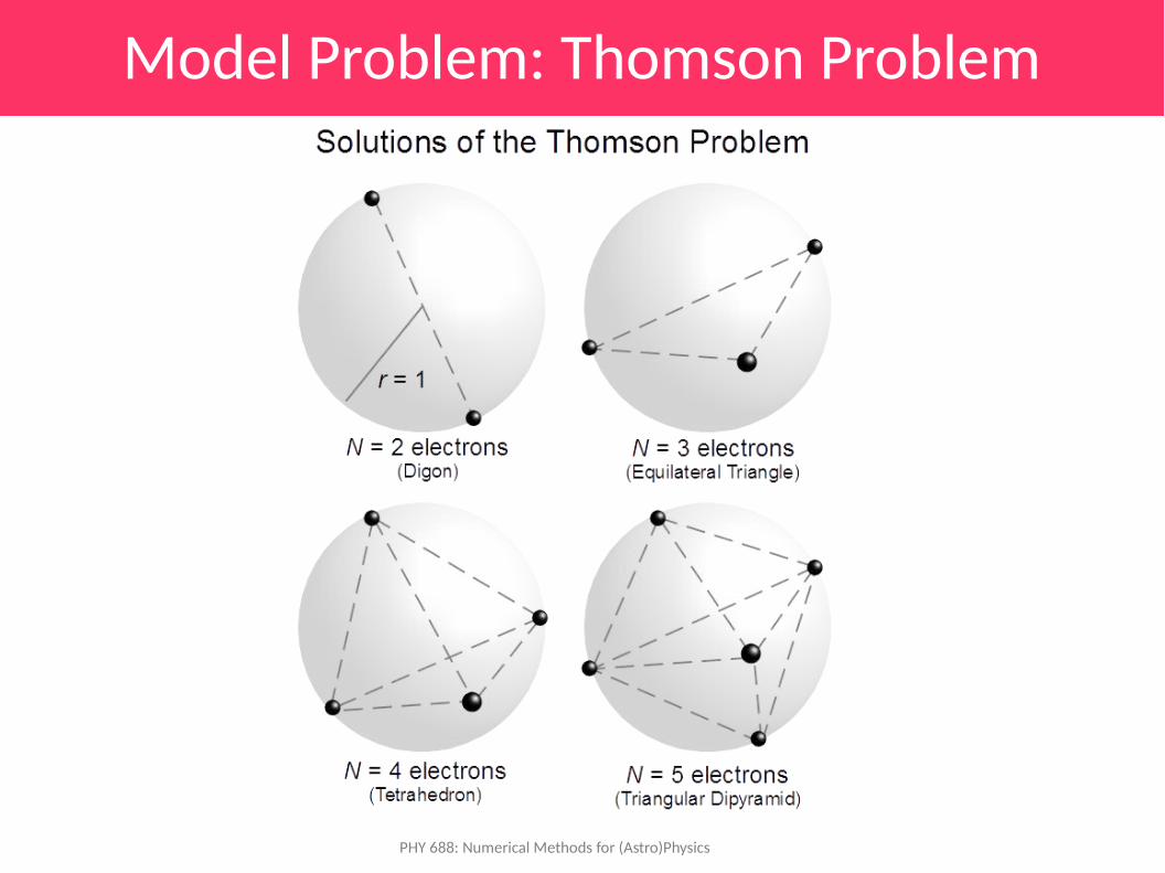
Model Problem: Thomson Problem● What's the minimum energy configuration for a finite number of

charges on the surface of a sphere?– Here, we minimize (in dimensionless units):


Model Problem: Thomson Problem● Minimum energy solutions have only been derived for (see

Wikipedia):– N = 1: trivial– N = 2: antipodal– N = 3: equilateral triangle on a great circle– N = 4: regular tetrahedron– N = 5: (only solved in 2010) triangular dipyramid– N = 6: regular octahedron– N = 12: regular icosahedron


Model Problem: Thomson Problem


Thomson Problem

(Wikipedia)


Binary Algorithm● At the heart of the genetic algorithm is encoding a list of parameters

into a chromosome– We'll restrict each parameter, ri to [0, 1]

● We'll translate each parameter into a binary (0 or 1) array– We pick the number of bits for each parameter—this will limit

precision– Our chromosome will be a concatenation of the binary parameters


Binary Algorithm● Encoding r in [0, 1] into m bits:

– Maximum error is then

● Encoding algorithm becomes:

Note: these expressions differ slightly from Pang because we are using 0-based indexing


Encoding and Decoding● Example of encoding then decoding

r 4 bits 6 bits 8 bits 10 bits 15 bits 20 bits 0.9505782217 | 0.9375000000 0.9375000000 0.9492187500 0.9501953125 0.9505615234 0.9505777359 0.5210286970 | 0.5000000000 0.5156250000 0.5195312500 0.5205078125 0.5210266113 0.5210285187 0.6374414473 | 0.6250000000 0.6250000000 0.6367187500 0.6367187500 0.6374206543 0.6374406815 0.1691710599 | 0.1250000000 0.1562500000 0.1679687500 0.1689453125 0.1691589355 0.1691703796 0.2993852393 | 0.2500000000 0.2968750000 0.2968750000 0.2988281250 0.2993774414 0.2993850708 0.0975094218 | 0.0625000000 0.0937500000 0.0937500000 0.0966796875 0.0975036621 0.0975093842 0.4987042499 | 0.4375000000 0.4843750000 0.4960937500 0.4980468750 0.4986877441 0.4987039566 0.4999217383 | 0.4375000000 0.4843750000 0.4960937500 0.4990234375 0.4999084473 0.4999208450 0.7376316858 | 0.6875000000 0.7343750000 0.7343750000 0.7373046875 0.7376098633 0.7376308441 0.4990126808 | 0.4375000000 0.4843750000 0.4960937500 0.4980468750 0.4989929199 0.4990119934

code: encode_decode.py


Encoding and Decoding● We have a vector, r, to encode for each realization of our problem● Encode each number and concatenate together to form the

chromosome● Ex: r = [0.125, 0.35, 0.9]

– Encoding (m = 5) gives the chromosome: [0 0 1 0 0 0 1 0 1 1 1 1 1 0 0]Decoding gives: [0.125, 0.34375, 0.875]

r0 r

1 r

2

code: chromosphere.py


Overview of GA● Create a population

– N different realizations: creatures, organisms, phenotypes– Randomly pick parameters and encode into a chromosome

● Select parents– The fittest of the population should “breed” and create the next

generation● Crossover

– Swap genes between the parent chromosomes to create the children● Mutation

– Randomly change some bits to introduce new data into the population


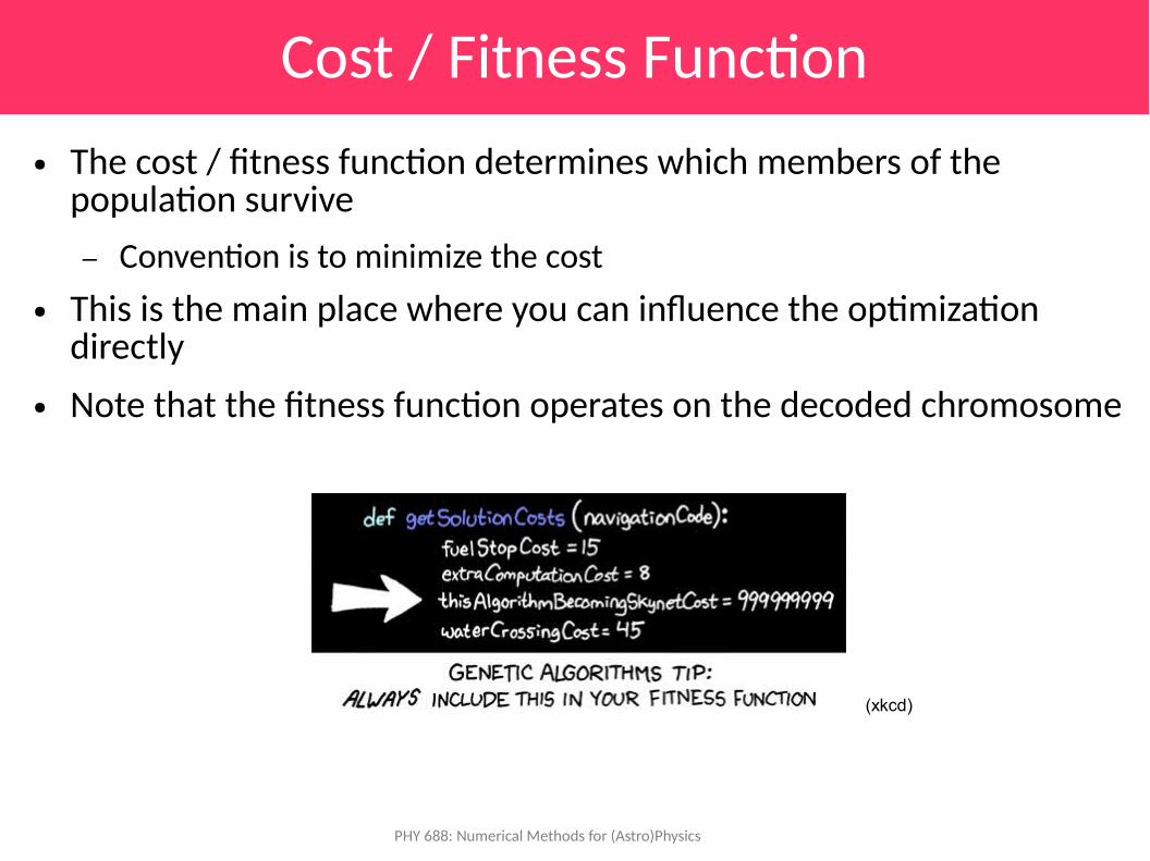
Cost / Fitness Function● The cost / fitness function determines which members of the

population survive– Convention is to minimize the cost

● This is the main place where you can influence the optimization directly

● Note that the fitness function operates on the decoded chromosome

(xkcd)


Initialization● We want a population of N creatures

– For the Thomson problem, each creature needs 2 parameters: spherical angles theta, phi

● Some variation: create 2N and keep the N fittest– We'll need a sorting method → order according to cost function

● Create the initial parameters for each creature via a random number generator (restricted to [0, 1))– Encode these to form the initial chromosome


Selection● We want to create a new population from the existing one

– Fittest creatures should have the biggest influence– Variations:

● Completely new population (N children)● N/2 parents create N/2 children (½ of previous population survives)● Some fraction of the fittest survive, the remainder breed

● There are a number of different ways we can select the parents– Keep the N/2 fittest, have them breed– Run a tournament: randomly pair 2 creatures and keep the fittest– Select pairs according to a probability (either based on rank or fitness),

e.g.:


Crossover● Parents create children by swapping parts of their genome

– Simplest method is crossover: ● Pick a dividing point in the chromosome● Cut parent chromosome at dividing point● Children are created by combining pieces of parents

– Ex: crossover point at the middle

Parent 1: 01101001010101 Parent 2: 10100111100111Child 1: 01101001100111 Child 2: 10100111010101


Mutation● Your crossover may never introduce new values of parameters, if you

cut the chromosome right at a boundary of parameters● Mutation can introduce more genetic diversity (just like in nature)● This is an essential part of the algorithm● Some variations:

– Mutate before or after crossover?– Keep the best (elite) creatures unmutated?

● Basic parameters:– Pick a mutation percentage– Flip bits in the chromosome based on the probability of mutation


Overall algorithm● Basic flow:

– Create the initial population– Do Ng generations:

● Select parents● Perform crossover● Do mutation


Thomson Problem● For the Thomson problem:

– Encode 2 parameters per charge●

– Total number of parameters per creature = 2 x # of charges● Cost function computes for the charge distribution of a creature:

– Without a loss of generality, we can put the first charge at the north pole and the second in the x-z plane


Thomson Problem● 5 charges: we find with N = 20 and 2000 generations:

– U = 6.47469238129 → this is pretty close to the right answer

code: thomson.py, genetic.py


Thomson Problem● 8 charges: we find with N = 20 and 10000 generations:

– U = 19.7502689737 → this is slightly off from the right answer



Variations● Mutation rate, population size, … all can affect the performance● At the core, we have a random process, so running several

realizations will show uncertainty

● The code is a little complicated—let's go over it– We'll view the output interactively so we can rotate it around



Genetic Cars● Here's a cool online example: genetic cars

– http://rednuht.org/genetic_cars_2/● Optimizes the design of a car using a genome consisting of:

– Shape: (8 genes, 1 per vertex)– Wheel size: (2 genes, 1 per wheel)– Wheel position: (2 genes, 1 per wheel)– Wheel density: (2 genes, 1 per wheel) darker wheels mean denser

wheels– Chassis density: (1 gene) darker body means denser chassis

http://rednuht.org/genetic_cars_2/


Continuous Algorithm● Chromosome is an array of real numbers

– Not converted into a bit representation● No longer need encode and decode methods● Selection is largely unchanged, since the cost function operates on

the real parameters already● Crossover:

– Simplest: cut the array at a boundary of elements and swap● In our binary method, we could conceivably cut a parameter's

representation and swap it, resulting in a completely new value of that parameter

– Some methods exist which allow for the real numbers themselves to be changed


Continuous Algorithm● Mutation: this can actually change the parameters

– Simplest method: just call a random number generator to change one of the parameters according to the mutation probability

● Benefits:– Should be faster, since we avoid all the encoding and decoding– Has better precision (since double precision numbers use 64 bits

instead of the m ~ 20 we were using with the binary algorithm)


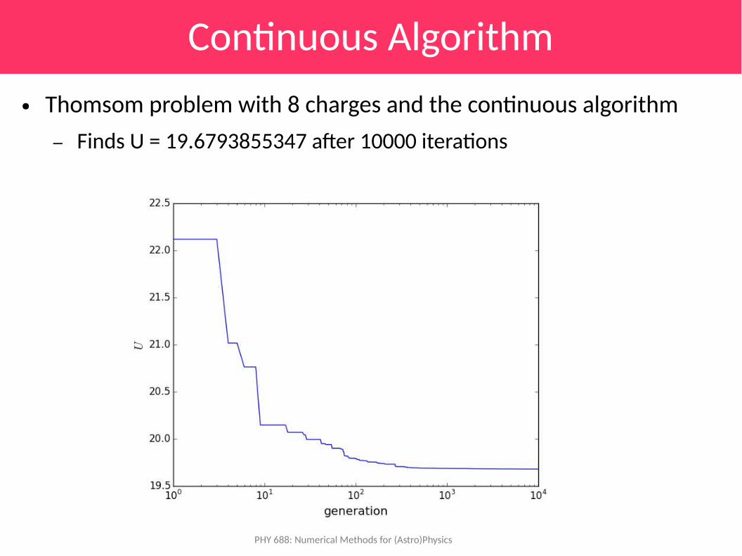
Continuous Algorithm● Thomsom problem with 8 charges and the continuous algorithm

– Finds U = 19.6793855347 after 10000 iterations


Binary vs. Continuous● Which should you use, binary or continuous?

– If your problem parameters are real numbers, probably continuous– If you problem parameters are discrete, then the binary version can

work well● See Gaffnet et al.


Simulated Annealing vs. GA?● Both simulated annealing and genetic algorithms can be used for

optimization problems– Both have the strength that the random nature helps avoid local

minima– Folklore seems to suggest that simulated annealing is the faster /

preferred method

Date post:	05-Apr-2018
Category:	Documents
Upload:	hoanghanh
View:	222 times
Download:	1 times

Genetic Algorithmsbender.astro.sunysb.edu/classes/phy688_spring2013/lectures/genetic.pdfPHY 688:...

Documents