Genetic gain increases by applying the usefulnesscriterion with improved variance prediction in selection
of crossesChristina Lehermeier∗,1, Simon Teyssèdre† and Chris-Carolin Schön∗
∗Plant Breeding, Technical University of Munich, 85354 Freising, Germany, †RAGT 2n, Genetics & Analytics Unit, 12510 Druelle, France
ABSTRACT A crucial step in plant breeding is the selection and combination of parents to form new crosses. Genome-basedprediction guides the selection of high-performing parental lines in many crop breeding programs which ensures a high meanperformance of progeny. To warrant maximum selection progress, a new cross should also provide a large progeny variance.The usefulness concept as measure of the gain that can be obtained from a specific cross accounts for variation in progenyvariance. Here, it is shown that genetic gain can be considerably increased when crosses are selected based on their genomicusefulness criterion compared to selection based on mean genomic estimated breeding values. An efficient and improvedmethod to predict the genetic variance of a cross based on Markov chain Monte Carlo samples of marker effects from awhole-genome regression model is suggested. In simulations representing selection procedures in crop breeding programs,the performance of this novel approach is compared with existing methods like selection based on mean genomic estimatedbreeding values and optimal haploid values. In all cases, higher genetic gain was obtained compared with previously suggestedmethods. When 1% of progenies per cross were selected, the genetic gain based on the estimated usefulness criterionincreased by 0.14 genetic standard deviations compared to a selection based on mean genomic estimated breeding values.Analytical derivations of the progeny genotypic variance-covariance matrix based on parental genotypes and genetic mapinformation make simulations of progeny dispensable and allow fast implementation in large-scale breeding programs.
In plant breeding superior inbred lines are developed either fordirect cultivar release, as hybrid components, or as potential
parents in population improvement. Generally, high yieldingparental lines are crossed to secure a high mean performance ofthe progeny. To identify superior progeny, ensure genetic gainin the next selection cycle, and to maintain long-term selectiongain, it is important that the cross also generates a high geneticvariance. Following Schnell and Utz (1975), the "usefulness" ofa cross is defined as the trait mean of a defined upper fractionof its progeny and can be derived as the expected cross meanplus the expected selection gain as a function of the selectionintensity, square-root of the trait heritability, and the genetic
standard deviation of the cross. With decreasing genotypingcosts, selection intensity can be increased by the use of genome-based prediction methods and consequently the importance ofconsidering the progeny variance when deciding about futurecrosses increases (Zhong and Jannink 2007). Several endeavorshave been made in the past to predict the progeny variance.Earlier attempts used the phenotypic distance (Utz et al. 2001)and since the availability of markers the molecular distance ofparental lines to predict progeny variance but both with limitedsuccess (Bohn et al. 1999; Hung et al. 2012). Recently, the poten-tial of genomic selection has been investigated for many speciesand in major crops such as maize and wheat it has been fullyintegrated in commercial breeding programs. The possibility toget dense marker genotypes allows an integration of genomicprediction in many steps of line and hybrid improvement pro-grams (Heslot et al. 2015). This has also led to the suggestionto use genomic estimated breeding values (GEBVs) to predict
Genetics, Vol. XXX, XXXX–XXXX October 2017 1
Genetics: Early Online, published on October 16, 2017 as 10.1534/genetics.117.300403
Copyright 2017.
the progeny variance (Bernardo 2014; Endelman 2011; Moham-madi et al. 2015). An R package developed by Mohammadi et al.(2015) predicts the progeny variance by using an appropriatetraining population of genotyped and phenotyped inbred linesand marker effects estimated with a whole-genome regressionmodel like ridge-regression best linear unbiased prediction (RR-BLUP, Meuwissen et al. (2001)). Subsequently, progenies fromtwo genotyped parental lines are simulated in silico using ge-netic map information. In a third step, GEBVs of the simulatedprogenies are predicted using marker effect estimates from thetraining population. The progeny variance is finally estimatedas sample variance of the GEBVs. Concerns about using thesample variance of GEBVs as estimate of the genetic variancewere raised as GEBVs are shrunken toward zero and thus theapproach underestimates the true genetic variance (Lian et al.2015). Lehermeier et al. (2017) showed that a fully Bayesianestimate as proposed by Sorensen et al. (2001) improves the esti-mation of the genetic variance explained by markers in a givenpopulation compared to estimation based on RR-BLUP variancecomponents by taking linkage disequilibrium (LD) betweenquantitative trait loci (QTL) into account. Here, we suggest tointegrate this fully Bayesian estimate of the genetic variance intothe usefulness criterion (UC).
Following a different rationale than the UC, Daetwyler et al.(2015) proposed the concept of selecting heterozygous linesbased on their optimal haploid value (OHV). The goal of OHVis to predict the best fully homozygous line that can be pro-duced from a heterozygous line or a cross. The authors showedthat selection based on OHV increases long-term genetic gaincompared to standard genomic selection based on GEBVs.
We hypothesize that an increase in genetic gain can be ob-tained when crosses are selected based on their estimated UCcompared to their mean GEBV or their OHV. In addition, ge-netic variance prediction is assumed to be more accurate witha fully Bayesian estimate based on MCMC samples comparedto the sample variance of the GEBVs. We investigate our hy-potheses in simulation studies based on genotypic maize dataunder varying selection intensities, trait heritabilities, trainingpopulation sizes, and model complexities. We show that thegenetic variance of progenies from a cross can be derived analyt-ically from the parental genotypes and genetic map informationwithout the need of in silico simulations. We provide formulasfor calculating the expected genetic variance for a given typeof population to be created from a biparental cross taking intoaccount the expected frequency of recombinants under differentlevels of inbreeding.
Material & Methods
Derivation of genetic variance among progeniesIn this section and supporting File S1, we show how to derivethe genetic variance of a cross under the assumption of biallelicQTL, known homozygous parental genotypes at QTL, knownQTL allele substitution effects, known recombination frequen-cies between QTL, and absence of dominance and epistasis. Wefirst concentrate on doubled haploid (DH) lines derived fromthe F1 generation of a biparental cross and then extend formu-las to general forms holding also for DH lines generated fromhigher selfing generations than F1 and to the genotypic varianceof recombinant inbred lines (RILs).
Two fully homozygous parental lines PA and PB are assumedwith known QTL genotypes xPA and xPB , each a vector of lengthNQTL counting the number of favorable QTL alleles at each of
NQTL QTL. We define the NQTL-dimensional vector of knownallele substitution effects as α. The breeding values of PA andPB are then x′PA
α and x′PBα. Further, DH progenies generated
from the F1 generation of a PA × PB cross are considered. Thegenotypes of the progenies can be defined as XPA×PB , a matrixwith progeny as rows and the NQTL QTL genotypes as columns.The mean breeding value of the progenies can be derived as themean of their parental lines’ breeding values:
µPA×PB =12(x′PA
α + x′PBα). (1)
The progeny variance can be derived as:
σ2PA×PB
= var(XPA×PB α) = α′var(XPA×PB )α. (2)
To obtain var(XPA×PB ), Bernardo (2014) and Mohammadiet al. (2015) suggested to simulate progenies in silico using theparental genotypes and a genetic map in order to obtain XPA×PB .If the approach is to be implemented in breeding programsto test the variance of a high number of potential crosses, thesimulation of progeny becomes a computationally intensive taskas per cross a minimum of several hundred progenies need tobe simulated for accurate variance estimation. In the following,we show how var(XPA×PB ) can be derived from the parentalgenotypes and the recombination frequencies without the needof simulating XPA×PB . For fully inbred lines it holds:
var(XPA×PB ) =
4π1(1− π1) · · · 4D1NQTL
.... . .
...
4DNQTL1 · · · 4πNQTL (1− πNQTL )
,
(3)
where the j-th diagonal entry corresponds to the varianceat the j-th QTL locus var(XPA×PB )jj = (1 + F)2πj(1− πj) withinbreeding coefficient F = 1 for fully inbred DH lines and πj theallele frequency in the parental lines which by expectation alsoholds for the progenies (πj ∈ {0, 0.5, 1}). For DH lines, the vari-ance at locus j is then either var(XPA×PB )jj = 1 if the parentalalleles differ at this locus or 0 if both parental lines have thesame allele and progenies will not show segregation at this locus.The off-diagonal elements of var(XPA×PB ) show the disequilib-rium covariances between two loci: var(XPA×PB )jl = 4Djl =
4(πjl − πjπl), where πjl denotes the haplotype frequency. Thedisequilibrium parameter Djl between loci j and l can be derivedfrom the disequilibrium parameter among both parental linesD∗jl and the expected frequency of recombinants between both
loci c(1)jl as: Djl = (1− 2c(1)jl )D∗jl . Depending on the parentalhaplotypes, D∗jl is either 0 if both parental lines show the samealleles at one or both loci, or 0.25 or -0.25 depending on the link-age phase of the parents. If DH lines are generated from a latergeneration than F1, it needs to be considered that the expectedfrequency of recombinants increases with increasing numberof meioses. Depending on the generation k when DH lines aregenerated (k = 1 for DH from F1), the expected frequency ofrecombinants increases to
c(k)jl =2c(1)jl
1 + 2c(1)jl
(1− 0.5k(1− 2c(1)jl )k). (4)
2 Lehermeier et al.
The general formula for DH lines generated from generationk is then:
var(XPA×PB )DH(k)jl = 4D∗jl(1− 2c(k)jl ). (5)
We give a full derivation for arriving at var(XPA×PB ) and anadjustment which also holds for recombinant inbred lines (RILs)after different numbers of selfing generations in the supportinginformation File S1. Table 1 summarizes how the genotypicvariance-covariance between two loci j and l can be derivedfor different populations based on the LD parameter D∗jl in theparental gametes and the expected frequency of recombinants
c(1)jl between both loci in the first generation.
Estimation of progeny variance based on whole-genome re-gressionFor estimating the variance of progeny, allele substitution effectsα need to be known. QTL and their effects cannot be observedbut with high marker density strong LD between markers andQTL can be exploited allowing to replace QTL with markergenotypes with only limited loss of information. We then can de-fine the marker genotypes MPA×PB and their NSNP-dimensionalvector of allele substitution effects β accordingly. Following Mo-hammadi et al. (2015) and Bernardo (2014) we estimate markereffects in a phenotyped and genotyped training population withthe linear regression model:
yTP = 1NTP β0 + MTPβ + ε, (6)
where yTP is the vector of phenotypes of a training popula-tion, β0 is an intercept, MTP is a matrix of marker genotypesof the individuals in the training population, β and ε the vec-tors of marker effects and residuals. We estimate marker effectsin a fully Bayesian way, assigning independent and identicalGaussian prior distributions to the marker effects β ∼ N(0, Iσ2
β).Residuals are also assumed to follow independent and identi-cal Gaussian distributions: ε ∼ N(0, Iσ2
ε ). Scaled inverse-χ2
prior distributions are assigned to the residual and marker effectvariance σ2
ε and σ2β. Samples from the posterior distribution
are created using a Markov chain Monte Carlo (MCMC) algo-rithm as implemented in the R package BGLR (Pérez and de losCampos 2014). Hyperparameters for the scaled inverse-χ2 priordistributions were chosen according to default rules in BGLRcorresponding to relatively uninformative priors and an a pri-ori assumption of 50% of the phenotypic variance explained bymarkers. We used 20,000 iterations, where the first 5000 sampleswere discarded as burn in. From the post burn in samples weonly saved every fifth sample for posterior inference correspond-ing to L = 3000 samples.
To estimate progeny variance based on the whole-genome re-gression model given in (6), two alternative methods were used.The first method which is denoted as the "variance of posteriormeans" (VPM) corresponds to calculating the sample varianceof the GEBVs g = MPA×PB β as described by Mohammadi et al.(2015) and Bernardo (2014) with
σ2[VPM]
PA×PB= var(MPA×PB β) = β
′var(MPA×PB )β, (7)
with β being the vector of posterior means of marker effectsobtained from model (6) using a training population.
Following Sorensen et al. (2001), the progeny variance can alsobe estimated by constructing a posterior distribution calculatingin each MCMC sample the progeny variance as:
where β(s) is the s-th thinned post burn in sample from theMCMC algorithm. By using the posterior mean from all sampleswe obtain the estimate according to method M2 of Lehermeieret al. (2017), which we denote here as the "posterior mean vari-ance" (PMV):
where var(β | yTP) is the posterior variance-covariance ma-trix of marker effects which is estimated based on L MCMCsamples: var(β | yTP) = 1/L · B′B, with B the L × NSNP-dimensional matrix of L samples of the NSNP marker effectscentered by their posterior means. The second part of equation(10) corresponds to σ2[VPM]
PA×PB(7) which can be interpreted as the
variation among GEBVs. The first part of equation (10) can be in-terpreted as variation of an individual’s GEBV originating fromvariation of marker effect estimates. If there is no uncertaintyin marker effect estimates, var(β | yTP) = 0 and the first part iszero. In this case, estimates from PMV and VPM are equal andshould approach the true genetic variance.
Usefulness and optimal haploid value of a crossAs in breeding the interest is typically both, increasing the meanof a population and identifying superior lines, crosses can beselected based on their UC (Schnell and Utz 1975) or their su-perior progeny value as defined by Zhong and Jannink (2007),which is the mean of the upper fraction of the selected lines. Fora normally distributed trait, the mean of the genotypic values ofselected progenies from a cross is:
UC = µ + iσg, (11)
with µ the genotypic mean of the cross, i the selection inten-sity (Falconer and Mackay 1996), and σg the genetic standard de-viation. Under absence of dominance and epistasis as assumedhere, the genotypic value of a line equals its breeding value.We predicted the usefulness of crosses by estimating µ from themean parental GEBVs and σg using the two alternative varianceestimation methods VPM and PMV as described in the previoussection. The genotypic variance-covariance matrix var(MPA×PB )entering VPM and PMV was derived from parental genotypesand genetic map information using the formula given in Table 1,line 1.
Variance prediction 3
Table 1 Overview of genotypic covariance between loci j and l for different populations derived from two parental lines basedon linkage disequilibrium parameter in parental lines D∗jl and expected frequency of recombinants in generation 1 c(1)jl .
Population Genotypic variance-covariance var(XPA×PB )jl
DH F1 (k = 1) a 4D∗jl(1− 2c(1)jl )
DH generation k 4D∗jl
(∑k
r=1
(0.5(1− 2c(1)jl )
)r+(
0.5(1− 2c(1)jl ))k)
RILs generation k b 4D∗jl(
∑kr=1
(0.5(1− 2c(1)jl )
)r)DH and RILs generation ∞ 4D∗jl
(1−
4c(1)jl
1+2c(1)jl
)a Doubled haploid (DH) lines derived from F1 generationb Recombinant inbred lines (RILs) after k− 1 selfing generations (k = 1 equals F2 population)
For comparison, we also investigated the concept of optimalhaploid value selection suggested by Daetwyler et al. (2015) toidentify superior crosses. We predicted the optimal haploidvalue that can be generated from a cross by:
OHV = 2NSegments
∑w=1
max(Hw βw), (12)
where NSegments is the number of segments in which thegenome is split to calculate the OHV, Hw defines a matrix withnumber of columns equal to the number of marker loci in seg-ment w and rows containing the four haplotype scores (0 or 1)of the two parental lines, and β
wdefines the vector containing
the marker effects of segment w estimated in model (6) using atraining population. Note, for fully homozygous parental lines,Hw can be reduced to two rows by considering one gamete each.In our study we split each chromosome in three segments cor-responding to the default value as chosen by Daetwyler et al.(2015).
Simulations
Our simulation study consists of two main parts. In the firstpart we investigate the two variance estimation methods (VPMand PMV) and in the second part we assess the genetic gainfrom selection based on UC and OHV compared to selectionbased on mean GEBVs. For both we simulated a trainingpopulation based on genotypic data from 10 multi-parentalpopulations of maize DH lines from the dent heterotic group,which were published by Bauer et al. (2013). The 841 DHlines were genotyped with the Illumina MaizeSNP50 Bead-Chip. After quality control and imputation of missing valuesas described by Lehermeier et al. (2014), 32,801 high-qualitypolymorphic SNPs were available and formed the genotypicdata of our training population. A genetic consensus mapof the 10 biparental families was constructed by Giraud et al.(2014) and is available at Maize GDB (http://maizegdb.org/cgi-bin/displayrefrecord.cgi?id=9024747). Based on this geneticmap information, recombination frequencies between markerpairs were derived as c(1) = 0.5(1− exp(−2x)), with x beingthe map distance between two marker loci in Morgan (Haldane1919).
Simulation Part 1 - Investigation of variance prediction meth-ods: We randomly sampled NQTL = 300 loci from the markerdata of the training population to be QTL and randomly sampled
QTL effects α from independent and identical normal distribu-tions with mean zero. True genotypic effects of the trainingpopulation were then defined as gTP = XTPα with XTP the QTLgenotypes of the training population. To obtain phenotypic val-ues, random error terms were sampled from a normal distribu-tion with mean zero and variance equal to var(gTP)(1− h2)/h2
to obtain a heritability of h2. Heritability values varied from 0.2to 1 in steps of 0.2. To investigate different training populationsizes, subsets varying in size from 100 to 600 in steps of 100were sampled randomly from the full training population. Anonly-QTL scenario and an only-marker scenario were consid-ered. In the only-QTL scenario we exclusively included the 300markers assigned a non-zero QTL effect in the whole-genomeregression model. This can be considered as ideal situation. Inthe only-marker scenario we excluded the 300 markers assignedQTL effects and included a random subset of 3000 remainingmarkers in the whole-genome regression model. Model parame-ters were then estimated using the specified training population.We generated 200 crosses among randomly sampled lines fromthe training population. In each cross, we calculated the true ge-netic variance as in equation (2) using the formula given in Table1 for DH lines derived from the F1 generation. Further, vari-ances were estimated using VPM and PMV as described abovewith their average bias calculated as true variance minus theestimated variance and standardized by the true variance. Thepredictive correlation of the variance estimates was calculatedas correlation between true variance and estimated varianceamong the 200 crosses. The whole simulation approach wasreplicated 10 times and results of bias and predictive correlationwere averaged over the 10 replications.
Simulation Part 2 - Selection based on UC and OHV: The simu-lation part 2 was based on a training population as simulated inpart 1 with training population size of NTP = 500, NQTL = 300and two different heritability values (h2 = 0.2 and 0.6). Usingonly 3000 non-QTL markers as in the only-marker scenario ofsimulation part 1, we fitted a whole-genome regression model asdescribed in equation (6). From the model we obtained GEBVsfor all lines in the training population. Using the GEBVs, weselected the 100 best lines (showing largest GEBVs) to formparental lines for new crosses. We calculated the mean of theGEBVs for all 4950 potential crosses of the 100 best lines. Fur-ther, we calculated the Rogers’ distance based on marker databetween the parental lines of the 4950 crosses. To avoid crossesbetween closely related parents and to ensure high means of thecrosses, we selected those crosses where parental lines showed aminimum genetic distance of 0.2 and subsequently selected the
4 Lehermeier et al.
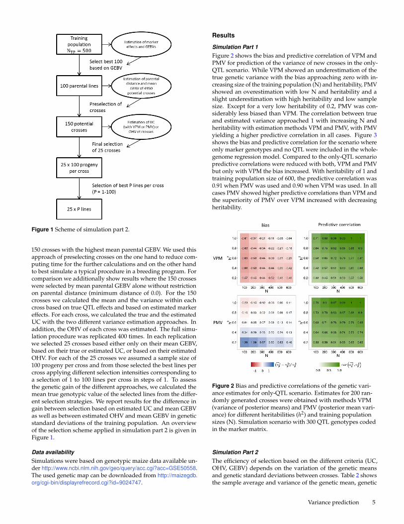
Figure 1 Scheme of simulation part 2.
150 crosses with the highest mean parental GEBV. We used thisapproach of preselecting crosses on the one hand to reduce com-puting time for the further calculations and on the other handto best simulate a typical procedure in a breeding program. Forcomparison we additionally show results where the 150 crosseswere selected by mean parental GEBV alone without restrictionon parental distance (minimum distance of 0.0). For the 150crosses we calculated the mean and the variance within eachcross based on true QTL effects and based on estimated markereffects. For each cross, we calculated the true and the estimatedUC with the two different variance estimation approaches. Inaddition, the OHV of each cross was estimated. The full simu-lation procedure was replicated 400 times. In each replicationwe selected 25 crosses based either only on their mean GEBV,based on their true or estimated UC, or based on their estimatedOHV. For each of the 25 crosses we assumed a sample size of100 progeny per cross and from those selected the best lines percross applying different selection intensities corresponding toa selection of 1 to 100 lines per cross in steps of 1. To assessthe genetic gain of the different approaches, we calculated themean true genotypic value of the selected lines from the differ-ent selection strategies. We report results for the difference ingain between selection based on estimated UC and mean GEBVas well as between estimated OHV and mean GEBV in geneticstandard deviations of the training population. An overviewof the selection scheme applied in simulation part 2 is given inFigure 1.
Data availabilitySimulations were based on genotypic maize data available un-der http://www.ncbi.nlm.nih.gov/geo/query/acc.cgi?acc=GSE50558.The used genetic map can be downloaded from http://maizegdb.org/cgi-bin/displayrefrecord.cgi?id=9024747.
Results
Simulation Part 1Figure 2 shows the bias and predictive correlation of VPM andPMV for prediction of the variance of new crosses in the only-QTL scenario. While VPM showed an underestimation of thetrue genetic variance with the bias approaching zero with in-creasing size of the training population (N) and heritability, PMVshowed an overestimation with low N and heritability and aslight underestimation with high heritability and low samplesize. Except for a very low heritability of 0.2, PMV was con-siderably less biased than VPM. The correlation between trueand estimated variance approached 1 with increasing N andheritability with estimation methods VPM and PMV, with PMVyielding a higher predictive correlation in all cases. Figure 3shows the bias and predictive correlation for the scenario whereonly marker genotypes and no QTL were included in the whole-genome regression model. Compared to the only-QTL scenariopredictive correlations were reduced with both, VPM and PMVbut only with VPM the bias increased. With heritability of 1 andtraining population size of 600, the predictive correlation was0.91 when PMV was used and 0.90 when VPM was used. In allcases PMV showed higher predictive correlations than VPM andthe superiority of PMV over VPM increased with decreasingheritability.
Figure 2 Bias and predictive correlations of the genetic vari-ance estimates for only-QTL scenario. Estimates for 200 ran-domly generated crosses were obtained with methods VPM(variance of posterior means) and PMV (posterior mean vari-ance) for different heritabilities (h2) and training populationsizes (N). Simulation scenario with 300 QTL genotypes codedin the marker matrix.
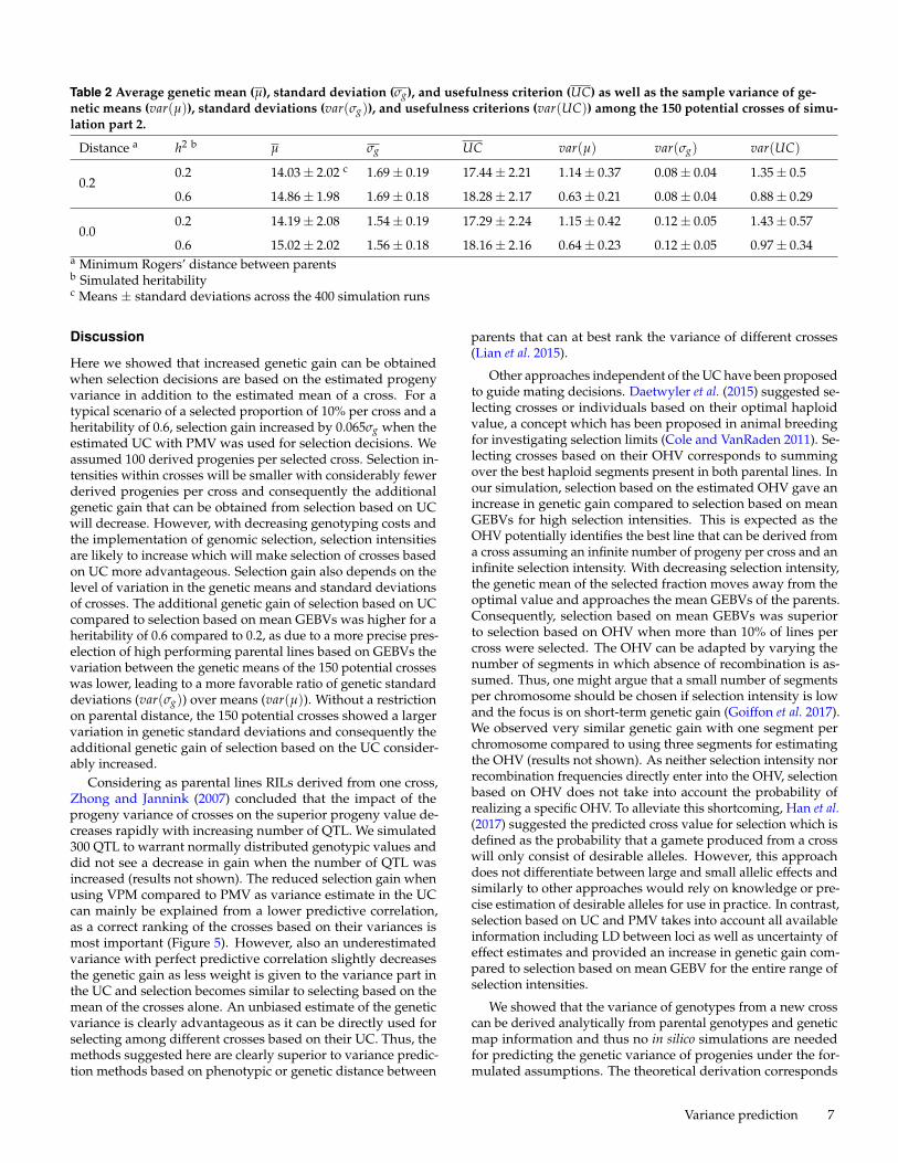
Simulation Part 2The efficiency of selection based on the different criteria (UC,OHV, GEBV) depends on the variation of the genetic meansand genetic standard deviations between crosses. Table 2 showsthe sample average and variance of the genetic mean, genetic
Figure 3 Bias and predictive correlations of the genetic vari-ance estimates for only-marker scenario. Estimates for 200randomly generated crosses were obtained with methodsVPM (variance of posterior means) and PMV (posterior meanvariance) for different heritabilities (h2) and training popula-tion sizes (N). Simulation scenario with 3000 non-QTL markergenotypes coded in the marker matrix.
standard deviation, and UC of the 150 crosses, preselected byparental GEBVs based on simulated heritabilities of 0.2 and 0.6and with a minimum distance between parents of 0.2 and 0.0.The average genetic mean and consequently the average UCincreased with higher heritability as the preselection by GEBVsselected high performing lines more reliably. The average withincross genetic standard deviation was only marginally affectedby the heritability. Similarly, the sample variance among crossgenetic means and the UC were smaller with higher heritabil-ity while the sample variance of genetic standard deviationsremained constant. Without restriction on parental distance, theaverage genetic mean increased but the average genetic standarddeviation and UC decreased. The sample variance of the geneticstandard deviations and UC increased compared to the fractionof crosses preselected based on a minimal parental distance of0.2.
Figure 4 shows the additional genetic gain that can be ob-tained when selection of crosses is based on the predicted UCor OHV compared to selection based on the mean GEBV of theparents as a function of the selection intensity within crossesfor heritabilities of 0.2 (Figure 4A) and 0.6 (Figure 4B) whencrosses were restricted to a minimum parental distance of 0.2.The additional gain of selection based on the UC increased withhigher selection intensities. For all heritabilities and selectionintensities, predicting UC based on PMV yielded the highestgenetic gain. When selecting only 1% of lines per cross and withheritability 0.6, the genetic gain increased up to 0.14σg. Withheritability of 0.6, estimating the variance with method PMVyielded up to 0.01σg more gain compared to using the varianceof posterior means (VPM) as estimate. With low heritability of0.2, the superiority of PMV over VPM increased up to 0.03σg. Se-
lecting crosses based on their OHV led to an increase in geneticgain compared to selection based on the mean GEBV for high se-lection intensity. When more than 10% progenies per cross wereselected, selection based on OHV was inferior to selection basedon mean GEBV. In general, selection based on estimated UC washighly superior to selection based on estimated OHV. With train-ing population heritability of 0.6, the additional genetic gain ofselecting crosses based on the UC compared to the mean GEBVwas higher than for a training population heritability of 0.2. Theadditional genetic gain of selection based on UC compared toselection based on mean GEBVs considerably increased whencrosses were not restricted to a minimum parental distance of0.2 and reached a maximum increase of 0.20σg for heritability0.2 (Figure 4C) and 0.24 for heritability 0.6 (Figure 4D).
Figure 5 shows the genetic gain when true UC and true OHVwere used for selection of crosses compared to selection basedon true mean genotypic values of parental lines consideringselection among 150 potential crosses preselected by minimumgenetic distance of 0.2 and heritability of 0.6 (comparable toFigure 4B). Here, QTL effects α were assumed to be known tocalculate the UC and OHV. With true effects the genetic gainfrom selection with UC increased up to 0.18σg. Similarly asunder the use of estimated marker effects, selection based ontrue OHV resulted in reduced gain compared to selection basedon true UC and was only superior to selection based on meangenotypic values when keeping less than 10% of progenies percross. In addition to selection based on true UC, Figure 5 showsselection based on artificially biased UC. For this the true ge-netic variance entering the UC was either divided by two tosimulate a variance estimate that is biased but has a predictivecorrelation of 1; or a random error was added to the true geneticvariance to simulate a variance estimate that is unbiased butshows predictive correlation of 0.5. A biased genetic variance inthe UC led to a small decrease in genetic gain of 0.01σg, while agenetic variance with a predictive correlation of 0.5 decreasedthe additional genetic gain by around one half.
6 Lehermeier et al.
Table 2 Average genetic mean (µ), standard deviation (σg), and usefulness criterion (UC) as well as the sample variance of ge-netic means (var(µ)), standard deviations (var(σg)), and usefulness criterions (var(UC)) among the 150 potential crosses of simu-lation part 2.
0.6 15.02± 2.02 1.56± 0.18 18.16± 2.16 0.64± 0.23 0.12± 0.05 0.97± 0.34a Minimum Rogers’ distance between parentsb Simulated heritabilityc Means ± standard deviations across the 400 simulation runs
Discussion
Here we showed that increased genetic gain can be obtainedwhen selection decisions are based on the estimated progenyvariance in addition to the estimated mean of a cross. For atypical scenario of a selected proportion of 10% per cross and aheritability of 0.6, selection gain increased by 0.065σg when theestimated UC with PMV was used for selection decisions. Weassumed 100 derived progenies per selected cross. Selection in-tensities within crosses will be smaller with considerably fewerderived progenies per cross and consequently the additionalgenetic gain that can be obtained from selection based on UCwill decrease. However, with decreasing genotyping costs andthe implementation of genomic selection, selection intensitiesare likely to increase which will make selection of crosses basedon UC more advantageous. Selection gain also depends on thelevel of variation in the genetic means and standard deviationsof crosses. The additional genetic gain of selection based on UCcompared to selection based on mean GEBVs was higher for aheritability of 0.6 compared to 0.2, as due to a more precise pres-election of high performing parental lines based on GEBVs thevariation between the genetic means of the 150 potential crosseswas lower, leading to a more favorable ratio of genetic standarddeviations (var(σg)) over means (var(µ)). Without a restrictionon parental distance, the 150 potential crosses showed a largervariation in genetic standard deviations and consequently theadditional genetic gain of selection based on the UC consider-ably increased.
Considering as parental lines RILs derived from one cross,Zhong and Jannink (2007) concluded that the impact of theprogeny variance of crosses on the superior progeny value de-creases rapidly with increasing number of QTL. We simulated300 QTL to warrant normally distributed genotypic values anddid not see a decrease in gain when the number of QTL wasincreased (results not shown). The reduced selection gain whenusing VPM compared to PMV as variance estimate in the UCcan mainly be explained from a lower predictive correlation,as a correct ranking of the crosses based on their variances ismost important (Figure 5). However, also an underestimatedvariance with perfect predictive correlation slightly decreasesthe genetic gain as less weight is given to the variance part inthe UC and selection becomes similar to selecting based on themean of the crosses alone. An unbiased estimate of the geneticvariance is clearly advantageous as it can be directly used forselecting among different crosses based on their UC. Thus, themethods suggested here are clearly superior to variance predic-tion methods based on phenotypic or genetic distance between
parents that can at best rank the variance of different crosses(Lian et al. 2015).
Other approaches independent of the UC have been proposedto guide mating decisions. Daetwyler et al. (2015) suggested se-lecting crosses or individuals based on their optimal haploidvalue, a concept which has been proposed in animal breedingfor investigating selection limits (Cole and VanRaden 2011). Se-lecting crosses based on their OHV corresponds to summingover the best haploid segments present in both parental lines. Inour simulation, selection based on the estimated OHV gave anincrease in genetic gain compared to selection based on meanGEBVs for high selection intensities. This is expected as theOHV potentially identifies the best line that can be derived froma cross assuming an infinite number of progeny per cross and aninfinite selection intensity. With decreasing selection intensity,the genetic mean of the selected fraction moves away from theoptimal value and approaches the mean GEBVs of the parents.Consequently, selection based on mean GEBVs was superiorto selection based on OHV when more than 10% of lines percross were selected. The OHV can be adapted by varying thenumber of segments in which absence of recombination is as-sumed. Thus, one might argue that a small number of segmentsper chromosome should be chosen if selection intensity is lowand the focus is on short-term genetic gain (Goiffon et al. 2017).We observed very similar genetic gain with one segment perchromosome compared to using three segments for estimatingthe OHV (results not shown). As neither selection intensity norrecombination frequencies directly enter into the OHV, selectionbased on OHV does not take into account the probability ofrealizing a specific OHV. To alleviate this shortcoming, Han et al.(2017) suggested the predicted cross value for selection which isdefined as the probability that a gamete produced from a crosswill only consist of desirable alleles. However, this approachdoes not differentiate between large and small allelic effects andsimilarly to other approaches would rely on knowledge or pre-cise estimation of desirable alleles for use in practice. In contrast,selection based on UC and PMV takes into account all availableinformation including LD between loci as well as uncertainty ofeffect estimates and provided an increase in genetic gain com-pared to selection based on mean GEBV for the entire range ofselection intensities.
We showed that the variance of genotypes from a new crosscan be derived analytically from parental genotypes and geneticmap information and thus no in silico simulations are neededfor predicting the genetic variance of progenies under the for-mulated assumptions. The theoretical derivation corresponds
Variance prediction 7
Figure 4 Additional gain of selecting crosses based on esti-mated usefulness criterion (UC) and optimal haploid value(OHV). Gain is given as the difference in mean genotypic val-ues of the selected lines from selection based on UC or OHVcompared to selecting based on mean GEBV alone, standard-ized by the true genotypic standard deviation σg in the train-ing population. Different variance estimates were used toestimate the UC (VPM, variance of posterior means; PMV,posterior mean variance). Gain is given for different fractionsof selected lines per cross. Results are shown for preselectedcrosses based on minimum Rogers’ distance between parentsof 0.2 and a heritability of 0.2 (A) and 0.6 (B) as well as forcrosses not preselected by parental distance and a heritabilityof 0.2 (C) and 0.6 (D).
Figure 5 Additionalgain of selecting crossesbased on true useful-ness criterion (UC), trueoptimal haploid value(OHV), or biased UC.For the biased UC ei-ther an underestimatedvariance (σ2
g = 0.5σ2g )
or a variance estimatewith predictive correla-tion of cor(σ2
g , σ2g) = 0.5
was considered. Gain isgiven in comparison togenetic gain when selec-tion was based on meanparental true genotypicvalues, standardized bythe genetic standard de-viation of the trainingpopulation.
to a simulation of an infinite number of progenies per cross andis most precise (see supporting File S1). The simulation of pro-genies can become computationally intense if the variance ofseveral thousands of crosses needs to be predicted so we con-sider our approach highly advantageous for application in abreeding program. One limitation of our approach is that forthe derivation of the progeny variance, assumptions regardingthe expected recombination frequency need to be made. Ourresults are based on the assumption of known recombination fre-quencies by assuming the given genetic map as true and absenceof interference (Haldane 1919). In practice, precision of esti-mated recombination frequencies might vary between speciesdepending on available mapping information and presence of in-terference. Furthermore, recombination rates might vary amongcrosses (Bauer et al. 2013), which might reduce the accuracyof variance prediction and consequently the superiority of theUC. All these limitations equally apply to both, the analyticalderivation of progeny variance as well as to in silico progenysimulations. The expected genetic variance depends on the pop-ulation type derived from a cross. Our results are focused onDH lines derived from the F1 generation of a cross but we givecomprehensive formulas also for different generations of RILsand DH lines considering the respective expected frequency ofrecombinants and different levels of inbreeding of the derivedpopulation. The specific formulas quantify if there is a gain ingenetic variance of a cross when DH lines are derived from alater generation than F1 (Sleper and Bernardo 2016) without theneed of additional time-consuming computations.
We investigated two different methods for predicting the ge-netic variance of newly generated crosses. Method VPM, thesample variance of the GEBVs, has been used for this and similarpurposes by other authors (Bernardo 2014; Mohammadi et al.2015; Segelke et al. 2014; Tiede et al. 2015; Wittenburg et al. 2016).As VPM is known to underestimate the true genetic variance asit is based on shrunken marker effect estimates (Cole and Van-Raden 2011; Lian et al. 2015), we investigated its performancefor obtaining accurate and precise progeny variance estimates
8 Lehermeier et al.
under different training population properties. In our study,VPM largely underestimated the true genetic variance with in-complete LD between markers and QTL (only-marker scenario).Only under ideal scenarios where markers were in perfect LDwith the QTL, the training population size largely exceeded thenumber of markers in the model, and when heritability was high,VPM provided a nearly unbiased estimate. The underestimationof VPM originates from the fact that uncertainty of the markereffect estimates is not taken into account. The posterior meanof the genetic variance calculated from MCMC samples (PMV)takes this uncertainty into account and consequently providedan improved variance estimator. As shown in equation (10), theestimated variance obtained from PMV can be split into the esti-mated variance obtained from VPM and a part that originatesfrom the marker effect variances. Accordingly, it yielded consis-tently larger variance estimates than VPM and showed only aslight deviation from the true genetic variance for heritabilityvalues above 0.2 in the only-QTL and only-marker scenario. Anoverestimation was observed for very low heritability, which canbe explained by model overfitting and large Monte Carlo errorsdue to the low signal-to-noise ratio in the training populationdata. As expected from theoretical considerations, variance esti-mates obtained from VPM and PMV converged with increasingheritability and training population size and both yielded a pre-dictive correlation of 1 in the more ideal scenarios (only QTL inthe model, h2 = 1, NTP = 600). Zhong and Jannink (2007) madea similar observation and found that a fully Bayesian treatmentof the superior progeny value was superior to using an approachbased on the posterior means of marker effects (comparable toVPM). It has been shown that for a given number of markers,increasing training population size and heritability increases theaccuracy of marker effect estimates (Wimmer et al. 2013). Ac-cordingly, as variance estimates obtained with VPM and PMVare based on marker effect estimates, they became more accu-rate with increasing heritability and training population size. Inagreement with the results of the predictive correlations, usingPMV always led to more genetic gain than using VPM and thissuperiority increased with decreasing heritability.
In our study we used an MCMC algorithm for obtaining bothvariance estimates (VPM and PMV). For VPM, MCMC wouldnot have been necessary and variance component estimatescould have been obtained with restricted maximum likelihood(REML). For PMV, an estimate for the variance-covariance ma-trix of the marker effects is needed. A closed form estimate forthis variance-covariance matrix can only be derived under anRR-BLUP model with known variance components σ2
β and σ2ε
and thus given shrinkage parameter λ = σ2ε /σ2
β, which is then
var(β | yTP, σ2β, σ2
ε ) = σ2ε (M ′M + λI)−1 M ′M(M ′M + λI)−T .
However, when variance components are unknown, no closedform exists and MCMC can be used to obtain an estimate. Al-ternatively, estimated variance components (e.g. from REML)might be plugged in to obtain var(β | yTP) but then the uncer-tainty of the variance component estimates is not taken intoaccount which might underestimate var(β | yTP) (Sorensen et al.2001). This approach would provide an alternative if one wantsto avoid using MCMC to save computing time. As expected,in our simulations this approach was superior considering pre-dictive correlation and bias compared to VPM but inferior com-pared to PMV (results not shown).
This study is based on simulations because a large num-ber of crosses and a large number of progenies per cross areneeded for inference. Such large numbers of unselected pro-
genies are rarely available in experimental breeding programs.Further, true genetic variances are unknown in experimentaldata and proper estimation requires replicated field trials totake genotype-by-environment interaction effects into accountwhich are typically large in maize (Acosta-Pech et al. 2017). Ourresults might represent an upper limit for the application of se-lecting crosses based on UC in practical breeding. Non-additiveor multi-allelic QTL effects which might affect the accuracy ofvariance prediction were not considered. We conjecture that theprediction of progeny variance is affected by non-additive andpopulation-specific effects similar to the prediction of breedingvalues where accuracies of methods are very similar irrespec-tive if non-additive effects are accounted for or not. In caseswhere non-additive effects are considered important, the whole-genome regression model to predict the genetic variance couldbe readily extended to include epistatic (Jiang and Reif 2015) orpopulation-specific effects (de los Campos et al. 2015; Lehermeieret al. 2015). In addition, Bayesian whole-genome regressionmodels including marker-specific shrinkage priors like BayesianLasso or BayesB could be used if large QTL effects are assumedto be segregating for the traits under study.
Predictions of the genetic variance are not only of interestfor selection of crosses in plant breeding but have also beenstudied in animal breeding for mating decisions (Bonk et al.2016; Segelke et al. 2014). We concentrated here on improvinga single trait in a directional selection approach. In general,knowledge of the genetic mean and variance of normally dis-tributed breeding values allows estimating the probability thatan offspring exceeds a specific threshold or that it is within aspecific range. Instead of increasing the genetic variance for fastselection progress, in specific situations the goal might lie in alarge mean combined with a low genetic variance for example inanimal breeding to obtain a homogeneous population (Cole andVanRaden 2011; Segelke et al. 2014). For such inferences and sub-sequent mating optimizations, an unbiased and precise varianceprediction as can be provided by PMV is important. The geneticvariance prediction can also be extended to the prediction ofgenetic covariances and correlations among multiple traits. Toestimate genetic correlations with PMV, genetic sample corre-lations among breeding values of two traits can be calculatedin each post burn in MCMC sample and from those posteriormeans can be formed. Further, the single-trait whole-genomeregression model could be extended to a multi-trait model toprofit from genetic correlations for the estimation of marker ef-fects (Jia and Jannink 2012). We conjecture that a multivariateextension of PMV also provides a superior prediction of geneticcorrelations between traits compared to VPM which warrantsfurther investigations. Knowledge of the genetic variance ofsingle traits and genetic correlations among multiple traits offuture crosses allows breeders to optimize their allocation of re-sources. Further, by applying formulas for different generationsof inbreeding it can be deduced how selection gain changes withadditional selfing steps. Here, our work provides a good startingpoint for the optimization of a genome-based prediction guidedbreeding program.
Literature Cited
Acosta-Pech, R., J. Crossa, G. de los Campos, S. Teyssèdre,B. Claustres, et al., 2017 Genomic models with genotype ×environment interaction for predicting hybrid performance:an application in maize hybrids. Theor. Appl. Genet. 130: 1431.
Variance prediction 9
Bauer, E., M. Falque, H. Walter, C. Bauland, C. Camisan, et al.,2013 Intraspecific variation of recombination rate in maize.Genome Biol. 14: R103.
Bernardo, R., 2014 Genomewide selection of parental inbreds:classes of loci and virtual biparental populations. Crop Sci. 54:2586–2595.
Bohn, M., H. F. Utz, and A. E. Melchinger, 1999 Genetic similari-ties among winter wheat cultivars determined on the basis ofRFLPs, AFLPs, and SSRs and their use for predicting progenyvariance. Crop Sci. 39: 228–237.
Bonk, S., M. Reichelt, F. Teuscher, D. Segelke, and N. Reinsch,2016 Mendelian sampling covariability of marker effects andgenetic values. Genet. Sel. Evol. 48: 36.
Cole, J. B. and P. M. VanRaden, 2011 Use of haplotypes to esti-mate Mendelian sampling effects and selection limits. J. Anim.Breed. Genet. 128: 446–455.
Daetwyler, H. D., M. J. Hayden, G. C. Spangenberg, and B. J.Hayes, 2015 Selection on optimal haploid value increases ge-netic gain and preserves more genetic diversity relative togenomic selection. Genetics 200: 1341–1348.
de los Campos, G., Y. Veturi, A. I. Vazquez, C. Lehermeier, andP. Pérez-Rodríguez, 2015 Incorporating genetic heterogeneityin whole-genome regressions using interactions. J. Agric. Biol.Envir. S. 20: 467–490.
Endelman, J. B., 2011 Ridge regression and other kernels forgenomic selection with R package rrBLUP. Plant Gen. 4: 250–255.
Falconer, D. S. and T. F. C. Mackay, 1996 Introduction to quantita-tive genetics. Longman, Essex, England.
Giraud, H., C. Lehermeier, E. Bauer, M. Falque, V. Segura, et al.,2014 Linkage disequilibrium with linkage analysis of multilinecrosses reveals different multiallelic QTL for hybrid perfor-mance in the flint and dent heterotic groups of maize. Genetics198: 1717–1734.
Goiffon, M., A. Kusmec, L. Wang, G. Hu, and P. Schnable, 2017Improving response in genomic selection with a population-based Selection strategy: optimal population value selection.Genetics doi: 10.1534/genetics.116.197103.
Haldane, J., 1919 The combination of linkage values and thecalculation of distances between the loci of linked factors.Journal of Genetics 8: 299–309.
Han, Y., J. N. Cameron, L. Wang, and W. D. Beavis, 2017 Thepredicted cross value for genetic introgression of multiplealleles. Genetics 205: 1409–1423.
Heslot, N., J.-L. Jannink, and M. E. Sorrells, 2015 Perspectives forgenomic selection applications and research in plants. CropSci. 55: 1–12.
Hung, H.-Y., C. Browne, K. Guill, N. Coles, M. Eller, et al., 2012The relationship between parental genetic or phenotypic diver-gence and progeny variation in the maize nested associationmapping population. Heredity 108: 490–499.
Jia, Y. and J.-L. Jannink, 2012 Multiple-trait genomic selectionmethods increase genetic value prediction accuracy. Genetics192: 1513–1522.
Jiang, Y. and J. C. Reif, 2015 Modeling epistasis in genomicselection. Genetics 201: 759–768.
Lehermeier, C., G. de los Campos, V. Wimmer, and C.-C. Schön,2017 Genomic variance estimates: With or without disequilib-rium covariances? J. Anim. Breed. Genet. 134: 232–241.
Lehermeier, C., N. Krämer, E. Bauer, C. Bauland, C. Camisan,et al., 2014 Usefulness of multiparental populations of maize(Zea mays L.) for genome-based prediction. Genetics 198: 3–16.
Lehermeier, C., C.-C. Schön, and G. de los Campos, 2015 Assess-ment of genetic heterogeneity in structured plant populationsusing multivariate whole-genome regression models. Genetics201: 323–337.
Lian, L., A. Jacobson, S. Zhong, and R. Bernardo, 2015 Pre-diction of genetic variance in biparental maize populations:genomewide marker effects versus mean genetic variance inprior populations. Crop Sci. 55: 1181–1188.
Meuwissen, T. H. E., B. J. Hayes, and M. E. Goddard, 2001 Predic-tion of total genetic value using genome-wide dense markermaps. Genetics 157: 1819 –1829.
Mohammadi, M., T. Tiede, and K. P. Smith, 2015 PopVar: agenome-wide procedure for predicting genetic variance andcorrelated response in biparental breeding populations. CropSci. 55: 2068–2077.
Pérez, P. and G. de los Campos, 2014 Genome-wide regression& prediction with the BGLR statistical package. Genetics 198:483–495.
Schnell, F. W. and H. F. Utz, 1975 F1-Leistung und Elternwahlin der Züchtung von Selbstbefruchtern. In Bericht über dieArbeitstagung der Vereinigung Österreichischer Pflanzenzüchter,pp. 234–258, Gumpenstein, Österreich.
Segelke, D., F. Reinhardt, Z. Liu, and G. Thaller, 2014 Predictionof expected genetic variation within groups of offspring forinnovative mating schemes. Genet. Sel. Evol. 46: 42.
Sleper, J. A. and R. Bernardo, 2016 Recombination and geneticvariance among maize doubled haploids induced from F1 andF2 plants. Theor. Appl. Genet. 129: 2429–2436.
Sorensen, D., R. Fernando, and D. Gianola, 2001 Inferring the tra-jectory of genetic variance in the course of artificial selection.Genet. Res. 77: 83–94.
Tiede, T., L. Kumar, M. Mohammadi, and K. P. Smith, 2015 Pre-dicting genetic variance in bi-parental breeding populationsis more accurate when explicitly modeling the segregation ofinformative genomewide markers. Mol. Breeding 35: 199.
Utz, H. F., M. Bohn, and A. E. Melchinger, 2001 Predictingprogeny means and variances of winter wheat crosses fromphenotypic values of their parents. Crop Sci. 41: 1470–1478.
Wimmer, V., C. Lehermeier, T. Albrecht, H.-J. Auinger, Y. Wang,et al., 2013 Genome-wide prediction of traits with different ge-netic architecture through efficient variable selection. Genetics195: 573–587.
Wittenburg, D., F. Teuscher, J. Klosa, and N. Reinsch, 2016 Co-variance between genotypic effects and its use for genomicinference in half-sib families. G3: Genes, Genomes, Genet. 6:2761–2772.
Zhong, S. and J.-L. Jannink, 2007 Using quantitative trait lociresults to discriminate among crosses on the basis of theirprogeny mean and variance. Genetics 177: 567–576.