Geocenter motions from GPS: A unified observation model David A. Lavalle ´e, 1 Tonie van Dam, 2 Geoffrey Blewitt, 3,4 and Peter J. Clarke 1 Received 15 April 2005; revised 22 December 2005; accepted 4 January 2006; published 6 May 2006. [1] We test a unified observation model for estimating surface-loading-induced geocenter motion using GPS. In principle, this model is more complete than current methods, since both the translation and deformation of the network are modeled in a frame at the center of mass of the entire Earth system. Real and synthetic data for six different GPS analyses over the period 1997.25–2004.25 are used to (1) build a comprehensive appraisal of the errors and (2) compare this unified approach with the alternatives. The network shift approach is found to perform particularly poorly with GPS. Furthermore, erroneously estimating additional scale changes with this approach can suggest an apparently significant seasonal variation which is due to real loading. An alternative to the network shift approach involves modeling degree-1 and possibly higher-degree deformations of the solid Earth in a realization of the center of figure frame. This approach is shown to be more robust for unevenly distributed networks. We find that a unified approach gives the lowest formal error of geocenter motion, smaller differences from the true value when using synthetic data, the best agreement between five different GPS analyses, and the closest (submillimeter) agreement with the geocenter motion predicted from loading models and estimated using satellite laser ranging. For five different GPS analyses, best estimates of annual geocenter motion have a weighted root-mean-square agreement of 0.6, 0.6, and 0.8 mm in amplitude and 21°, 22°, and 22° in phase for x, y , and z, respectively. Citation: Lavalle ´e, D. A., T. van Dam, G. Blewitt, and P. J. Clarke (2006), Geocenter motions from GPS: A unified observation model, J. Geophys. Res., 111, B05405, doi:10.1029/2005JB003784. 1. Introduction [2] The mass contained in the Earth’s fluid envelope (oceans, atmosphere, and continental water) is constant at human timescales. However, its distribution over the surface of the Earth changes continually. Much of this geographic redistribution of surface mass happens periodically at 24 hour to annual periods and is related to the rotation of the Earth on its axis (e.g., thermally driven atmospheric tides) as well as motion of the Earth around the Sun (e.g., annual global water cycle). In the absence of external forces the center of mass of the entire solid Earth and load system (CM) is a fixed point in space; relative to this point a change in the location of the center of mass of the surface load must (by conservation of linear momentum) induce a change in the relative location of the center of mass of the solid Earth (CE). This ‘‘geocenter motion’’ causes a detectable transla- tion of a geodetic network attached to the solid Earth, relative to the center of satellite orbits, which is CM [Chen et al., 1999; Watkins and Eanes, 1993; Watkins and Eanes, 1997]. While geocenter motion is principally a product of mass balance relations, the geodetic network is located on the surface of the solid Earth which also deforms because of redistribution of the load. Thus the same process (redistri- bution of surface mass) is expressed in the geodetic network in two quite different ways: displacement of the Earth’s center related to mass balance and subsequent deformation of the solid Earth due to the load. For a totally rigid Earth, there would be no deformation; in an elastic Earth the deformational movement at a point can reach up to 40% of the magnitude of the geocenter trajectory and must be taken into account [Blewitt, 2003]. A graphical representa- tion of these concepts is given in Figure 1. [3] Estimates of geocenter motion from space geodesy are important since they fundamentally relate to how we realize the terrestrial reference frame [Blewitt, 2003; Dong et al., 2003]. Conventionally, the center of the International Terrestrial Reference Frame (ITRF) is defined to be at the center of mass of the entire Earth system, i.e., CM [McCarthy and Petit, 2004]. Estimates of geocenter motion can also help to constrain models involving global redistri- bution of mass [Chen et al., 1999; Cretaux et al., 2002; Dong et al., 1997] and sea level [Blewitt and Clarke, 2003], since they are directly related to the degree-1 component of the surface mass load. This is particularly relevant because current estimates of the degree-1 surface mass load derived JOURNAL OF GEOPHYSICAL RESEARCH, VOL. 111, B05405, doi:10.1029/2005JB003784, 2006 1 School of Civil Engineering and Geosciences, University of Newcastle upon Tyne, Newcastle, UK. 2 European Center for Geodynamics and Seismology, Walferdange, Luxembourg. 3 Nevada Bureau of Mines and Geology, University of Nevada, Reno, Nevada, USA. 4 Also at Nevada Seismological Laboratory, University of Nevada, Reno, Nevada, USA. Copyright 2006 by the American Geophysical Union. 0148-0227/06/2005JB003784$09.00 B05405 1 of 15
Transcript
Geocenter motions from GPS: A unified observation model
David A. Lavallee,1 Tonie van Dam,2 Geoffrey Blewitt,3,4 and Peter J. Clarke1
Received 15 April 2005; revised 22 December 2005; accepted 4 January 2006; published 6 May 2006.
[1] We test a unified observation model for estimating surface-loading-induced geocentermotion using GPS. In principle, this model is more complete than current methods,since both the translation and deformation of the network are modeled in a frame at thecenter of mass of the entire Earth system. Real and synthetic data for six differentGPS analyses over the period 1997.25–2004.25 are used to (1) build a comprehensiveappraisal of the errors and (2) compare this unified approach with the alternatives. Thenetwork shift approach is found to perform particularly poorly with GPS. Furthermore,erroneously estimating additional scale changes with this approach can suggest anapparently significant seasonal variation which is due to real loading. An alternative to thenetwork shift approach involves modeling degree-1 and possibly higher-degreedeformations of the solid Earth in a realization of the center of figure frame. This approachis shown to be more robust for unevenly distributed networks. We find that a unifiedapproach gives the lowest formal error of geocenter motion, smaller differences from thetrue value when using synthetic data, the best agreement between five different GPSanalyses, and the closest (submillimeter) agreement with the geocenter motion predictedfrom loading models and estimated using satellite laser ranging. For five different GPSanalyses, best estimates of annual geocenter motion have a weighted root-mean-squareagreement of 0.6, 0.6, and 0.8 mm in amplitude and 21�, 22�, and 22� in phase for x, y, andz, respectively.
Citation: Lavallee, D. A., T. van Dam, G. Blewitt, and P. J. Clarke (2006), Geocenter motions from GPS: A unified observation
model, J. Geophys. Res., 111, B05405, doi:10.1029/2005JB003784.
1. Introduction
[2] The mass contained in the Earth’s fluid envelope(oceans, atmosphere, and continental water) is constant athuman timescales. However, its distribution over the surfaceof the Earth changes continually. Much of this geographicredistribution of surface mass happens periodically at24 hour to annual periods and is related to the rotation ofthe Earth on its axis (e.g., thermally driven atmospherictides) as well as motion of the Earth around the Sun (e.g.,annual global water cycle). In the absence of external forcesthe center of mass of the entire solid Earth and load system(CM) is a fixed point in space; relative to this point a changein the location of the center of mass of the surface load must(by conservation of linear momentum) induce a change inthe relative location of the center of mass of the solid Earth(CE). This ‘‘geocenter motion’’ causes a detectable transla-tion of a geodetic network attached to the solid Earth,
relative to the center of satellite orbits, which is CM [Chenet al., 1999; Watkins and Eanes, 1993; Watkins and Eanes,1997]. While geocenter motion is principally a product ofmass balance relations, the geodetic network is located onthe surface of the solid Earth which also deforms because ofredistribution of the load. Thus the same process (redistri-bution of surface mass) is expressed in the geodetic networkin two quite different ways: displacement of the Earth’scenter related to mass balance and subsequent deformationof the solid Earth due to the load. For a totally rigid Earth,there would be no deformation; in an elastic Earth thedeformational movement at a point can reach up to 40%of the magnitude of the geocenter trajectory and must betaken into account [Blewitt, 2003]. A graphical representa-tion of these concepts is given in Figure 1.[3] Estimates of geocenter motion from space geodesy
are important since they fundamentally relate to how werealize the terrestrial reference frame [Blewitt, 2003; Donget al., 2003]. Conventionally, the center of the InternationalTerrestrial Reference Frame (ITRF) is defined to be atthe center of mass of the entire Earth system, i.e., CM[McCarthy and Petit, 2004]. Estimates of geocenter motioncan also help to constrain models involving global redistri-bution of mass [Chen et al., 1999; Cretaux et al., 2002;Dong et al., 1997] and sea level [Blewitt and Clarke, 2003],since they are directly related to the degree-1 component ofthe surface mass load. This is particularly relevant becausecurrent estimates of the degree-1 surface mass load derived
JOURNAL OF GEOPHYSICAL RESEARCH, VOL. 111, B05405, doi:10.1029/2005JB003784, 2006
1School of Civil Engineering and Geosciences, University of Newcastleupon Tyne, Newcastle, UK.
2European Center for Geodynamics and Seismology, Walferdange,Luxembourg.
3Nevada Bureau of Mines and Geology, University of Nevada, Reno,Nevada, USA.
4Also at Nevada Seismological Laboratory, University of Nevada,Reno, Nevada, USA.
Copyright 2006 by the American Geophysical Union.0148-0227/06/2005JB003784$09.00
B05405 1 of 15
from environmental models disagree. A number of authorsestimate the annual and semiannual components of geo-center motion induced by different models of surface massredistribution [Bouille et al., 2000; Chen et al., 1999;Cretaux et al., 2002; Dong et al., 1997; Moore and Wang,2003]. While the geocenter motions from different atmo-spheric mass models tend to agree for all components,significant differences (up to 50%) are observed in annualand semiannual geocenter motion from ocean bottom pres-sure and, more importantly, from continental water mass.The standard deviation about the mean of the modeledannual geocenter from 11 different model combinations[Bouille et al., 2000; Chen et al., 1999; Cretaux et al.,2002; Dong et al., 1997; Moore and Wang, 2003] suggeststhe precision of the modeled annual geocenter variation ison the order of �1 mm in amplitude and �20� in phase.[4] The Gravity Recovery and Climate Experiment
(GRACE) mission results [Tapley et al., 2004] will providesignificant new information on the surface mass variationsover the Earth down to periods of 1 month. However, theGRACE products do not include degree 1 to which GRACEis insensitive. The determination of degree-1 coefficients ofthe Earth’s surface mass load from observational data andthe discrimination of modeled environmental data sets istherefore left to other geodetic techniques such as satellitelaser ranging (SLR), Doppler orbitography and radioposi-tioning integrated by satellite (DORIS) and the GlobalPositioning System (GPS).[5] It should be noted that no geodetic estimates of
secular geocenter motion currently exist; tectonic deforma-tion will produce a net translation of the center of surfacefigure (CF) relative to the center of mass (CM) which isgenerally first removed by estimating tectonic velocities ateach site. Only if a plate rotation model is used can such anestimate be made and so far is considered systematicreference frame error rather than physical signal [Argus etal., 1999], much further work is required to solve thisimportant reference frame issue. In this work the estimationis considered for the more common use of the term ‘‘geo-center motion,’’ that is, assuming tectonic deformationhas been first removed. This work does not reflect theability of a network shift or Helmert transformationapproach to resolve the aforementioned reference frameissues associated with what might be called secular ‘‘geo-center motion’’ or even its ability to resolve secular differ-ences between reference frames.[6] There have been a number of different approaches to
estimating geocenter motions from geodetic measurements[Ray, 1999] including (1) the so-called ‘‘network shiftapproach’’ [Blewitt et al., 1992; Dong et al., 2003; Heflinand Watkins, 1999], also called the ‘‘geometric approach’’[Cheng, 1999; Pavlis, 1999], which directly models thetranslation between coordinate frames, (2) the ‘‘dynamicapproach’’ [Chen et al., 1999; Pavlis, 1999; Vigue et al.,1992], which estimates degree-1 coefficients of the geo-potential, and (3) the ‘‘degree-1 deformation’’ approach[Blewitt et al., 2001; Dong et al., 2003], which equatessolid Earth deformation caused by the load to geocentermotion. The dynamic and network shift approach areequivalent (where constraints are minimal), and in this workwe only consider the latter. We note that describing the‘‘network shift approach’’ as ‘‘geometric’’ is misleading
because this approach principally depends on satellitedynamics to locate the Earth center of mass and so isfundamentally a dynamic approach. Here we are consistentwith the terminology of Dong et al. [2003]. Lavallee andBlewitt [2002] show that even the nonsatellite technique ofvery long baseline interferometry (VLBI) is sensitive togeocenter motions via the degree-1 deformation. However,to quote Boucher and Sillard [1999], commenting on thegeocenter series submitted to the 1999 International EarthRotation Service (IERS) analysis campaign to investigatemotions of the geocenter, ‘‘It appears that, even if SpaceGeodesy geocenter estimates are sensitive to seasonalvariations, the determinations are not yet accurate andreliable enough to adopt an empirical model that wouldrepresent a real signal.’’ Disagreement between differentgeodetic analyses is still considerably larger than thatbetween loading models. Much of this disagreement comesfrom differences between GPS analyses; estimates fromSLR tracking of LAGEOS 1 and 2 [Bouille et al., 2000;Chen et al., 1999; Cretaux et al., 2002; Moore and Wang,2003] are in much better agreement.[7] The source of the disagreement between GPS analy-
ses has been difficult to track down; Dong et al. [2002] andWu et al. [2002] estimate the size of the error in the networkshift approach due to an imperfect network, and Wu et al.[2002] estimate aliasing errors in the degree-1 deformationapproach. A number of authors [Blewitt, 2003; Dong et al.,2003; Wu et al., 2002] state that the network shift approachis biased by deficiencies in GPS orbit modeling but aquantitative consideration of how all errors trades offagainst each other for different networks and approacheshas not been completed. Although Dong et al. [2003]suggest the degree-1 deformation approach produces morestable geocenter estimates, Wu et al. [2002] suggest theignored higher degrees produce a significant error. Thisuncertainty in how best to estimate geocenter motions fromGPS makes it difficult to recommend procedures for defin-ing the terrestrial reference frame [Ray et al., 2004] or makerobust inferences about degree-1 surface mass loading.Dong et al. [2003] even suggest that given the improvedprecision of modern geodetic techniques geocenter motionsshould be included in the definition of the ITRF as estima-ble parameters.[8] Current methods to model geocenter motion consider
either the translational or the deformation expression ofchange in the center of mass of the surface load; here we testa model that unifies these two aspects. In principle, this is abetter way to model geocenter motions: It is complete, inthat all the displacements associated with geocenter motionare modeled, and it is also conventional, such that displace-ments are modeled in the CM frame. We complete anappraisal of possible errors in the current geocenter motionestimation strategies applied to GPS and make a comparisonof the unified approach with these alternatives.
2. Estimating Geocenter Motions FromSpace Geodesy
[9] For mathematical convenience we define ‘‘geocentermotion’’ in the context of this paper as the 3-D vectordisplacement DrCF-CM of the center of surface figure (CF)of the solid Earth’s surface relative to the center of mass
B05405 LAVALLEE ET AL.: GEOCENTER MOTIONS FROM GPS
2 of 15
B05405
(CM) of the entire Earth system (solid Earth, oceans, andatmosphere). Although the term ‘‘geocenter motions’’ hasbeen used to describe the vector difference between anumber of frames [Blewitt, 2003; Dong et al., 1997],DrCF-CM or its opposite in sign (DrCM-CF) are the mostcommonly estimated geocenter parameters from GPS[Heflin et al., 2002; Malla et al., 1993; Ray, 1999; Vigueet al., 1992], SLR [Bouille et al., 2000; Chen et al., 1999;Cretaux et al., 2002; Moore and Wang, 2003], and DORIS[Bouille et al., 2000; Cretaux et al., 2002], so we treat it asthe desired estimable parameter. As discussed, the center ofmass of the solid Earth (CE) is displaced from CM becauseof the changing location of the center of mass of the load.CF is a useful point that represents the geometrical center ofthe Earth’s surface. It is displaced from CE because of thedeformation of the solid Earth accompanying loading; if theEarth were rigid, these points would coincide. Since CF isessentially the global average of the surface deformation, itdiffers in location to CE by only �2% [Blewitt, 2003];however, this can be misleading since at specific locationsthe deformational displacement can be on the order of 40%.[10] The three-dimensional displacement (east, north, and
up) of a point on the Earth’s surface due to surface massloading can be described [Diziewonski and Anderson, 1981;Farrell, 1972; Lambeck, 1980] using spherical harmonicexpansion and a spherically symmetric, layered, nonrota-tional and isotropic Earth model of the form
E Wð Þ ¼ rSrE
X1n¼1
Xnm¼0
XC;Sf g
F
3l0n2nþ 1ð ÞT
Fnm
@lYFnm Wð Þ
cosj
N Wð Þ ¼ rSrE
X1n¼1
Xnm¼0
XC;Sf g
F
3l0n2nþ 1ð ÞT
Fnm@jY
Fnm Wð Þ ð1Þ
H Wð Þ ¼ rSrE
X1n¼1
Xnm¼0
XC;Sf g
F
3h0n2nþ 1ð ÞT
FnmY
Fnm Wð Þ
where TnmF are the spherical harmonic coefficients of the
surface load density following the conventions of Blewittand Clarke [2003] and expressed as the height of a columnof seawater, h0n and l0n are the degree-n Love numberswhich for degree 1 must be specified in our chosen frame[Blewitt, 2003], rs is the density of seawater and rE is themean density of the Earth.[11] It can be shown [Trupin et al., 1992] that surface
integration of (1) gives the following geocenter motionbetween the CM and CF frames:
D~rCF-CM ¼h01� �
CEþ 2 l01
� �CE
� �3
1
0@
1A rs
rE
TC11
TS11
TC10
0BBBB@
1CCCCA ð2Þ
We choose to use CE frame Love numbers in (2) since
theh01� �
CEþ 2 l01
� �CE
� �3
1 term helps demonstrate the
concept of translation and then deformation of the solidEarth. The unity term is the translation from CM to CEwhich is much larger than the first term which describesthe average deformation of the solid Earth that displacesCF from CE. The first term has a magnitude of 0.021using the Love numbers of Farrell [1972]; it is importantto recall, however, that the deformation at a point givenby (1) can be much larger than this.
2.1. A Unified Observation Model
[12] A unified approach for geocenter motion modelsdisplacements in the CM frame at each site using (1), whereLove numbers are in the CM frame. In this way both thetranslation and deformation of the network are modeled.Strictly speaking, only the degree-1 deformation need bemodeled as the higher degrees do not relate to the center ofmass of the load. Higher-degree deformation will, however,be present in geodetic observations and could alias esti-mates of geocenter motion if not included, so it can bebeneficial to include some of them. For short we call thisunified model the ‘‘CM method.’’ The design matrix for thisapproach is given in Appendix A.[13] A note of caution must be attached to the CM
method when anything but a full weight matrix is usedduring estimation. Estimating the translational aspects ofgeocenter motions relies on determining the CM frame viasimultaneous solution for GPS satellite orbital dynamicsand coordinates of a global site network. This information ispresent in the off diagonal elements of the stochastic model;information on the determination of individual site coordi-nates relative to the network as a whole is given along thediagonal. It is the stochastic model that determines therelative influence of translation and deformation onthe estimate of geocenter motion. If the covariance matrixof observations is diagonal or block diagonal the translationof the network is effectively given a much larger weightthan the deformation and the CM method gives identicalresults to the network shift method.[14] This is particularly pertinent for GPS results obtained
using precise point positioning [Zumberge et al., 1997], inwhich orbits are fixed (considered perfect in the stochastic
Figure 1. Graphical representation of displacements with-in a geodetic network due to changing location of center ofmass of surface load. CM is center of mass of solid Earthplus load, the origin of satellite orbits which is essentially akinematic fixed point in space. Two quite differentexpressions are observed: displacement of center of solidEarth (CE) and deformation of solid Earth.
B05405 LAVALLEE ET AL.: GEOCENTER MOTIONS FROM GPS
3 of 15
B05405
model). While point positioning is a very useful approachfor regional analysis, it is generally not suitable for esti-mating global parameters such as geocenter motion. Theresults obtained will be identical to those from the networkshift approach for a global network and the same ascommon mode filtering [Wdowinski et al., 1997] on aregional scale. Davis et al. [2004] attempt to estimatedegree-1 deformation from continental-scale point-position-ing results in this manner so that the remaining higher-degree (>1) deformation can be compared to GRACEmeasurements. However, Davis et al. [2004] have removedonly a mean from their GPS results (and not the degree-1deformation), so this is equivalent to common mode filter-ing on a continental scale.
2.2. The Network Shift Approach
[15] Estimation of DrCF-CM from GPS measurements hasbeen most commonly performed by modeling displace-ments as a translation only [Heflin et al., 2002; Heflinand Watkins, 1999]. Generally, a least squares approach isused to estimate a Helmert transformation with up to sevenparameters [Blewitt et al., 1992]. We follow [Dong et al.,2003] in calling this the ‘‘network shift approach.’’ Thisapproach models only the translational aspect of geocentermotion, and it is easy to see how such a procedure could bedeveloped from (2) since the globally averaged deformationis very small. Modeling coordinate displacements as only atranslation, however, ignores the quite large deformationsthat can occur on a site by site basis and the estimate inreality defines a center of network (CN) frame [Wu et al.,2002] giving geocenter motion DrCN-CM which is only anapproximation of DrCF-CM.[16] When estimating a Helmert transformation it can be
necessary to estimate rotation parameters since in fiducial-free GPS analysis network orientation is only loosely con-strained [Heflin et al., 1992]; however, a scale parametershould not be estimated. A scale parameter is sometimesincluded when estimating Helmert transformations to inves-tigate any systematic differences in the definition of scalebetween different techniques, e.g., VLBI, SLR, GPS orDORIS [Altamimi et al., 2002]. When estimating DrCF-CM,however, there is no reason to include a scale parameter sincewe are using only one technique and the scale definition is thesame. An estimated scale parameter could absorb some of theloading deformation due to an imperfect (e.g., continentallybiased) network giving an apparent scale error; this error isunfortunate and can be completely avoided by not estimatingscale.
2.3. Degree-1 Deformation Approach
[17] Blewitt et al. [2001] estimate the degree-1 coeffi-cients of the surface mass load (expressed as the load massmoment) from GPS using a priori information about theEarth’s elastic properties given by the loading model spec-ified in (1) and the degree-1 Love numbers [Farrell, 1972]in the CF frame. By modeling only the deformation thetranslational aspect of geocenter motion does not influencethe estimate. Blewitt et al. [2001] model GPS displacementsin a realization of the CF frame with
Dsi½ �CF¼ GTdiag l01� �
CFl01� �
CFh01� �
CF
h iG
m
M ð3Þ
wherem is the ‘‘load moment,’’ [h01]CF and [l01]CF are degree-1
Love numbers in the CF frame, and for simplification theheight and lateral degree-1 spherical harmonic functions (1)are identified with the elements of the geocentric totopocentric rotation matrix G (Appendix A). In the notationof this paper this is identical to (1) for the CF frame where weidentify
m
M ¼ rs
rE
TC11
TS11
TC10
0@
1A ð4Þ
and hence (3) is a method to estimate DrCF-CM through (2).[Dong et al., 2003] named this the ‘‘degree-1 deformation’’approach; this is an alternative method to the network shiftbut is dependent on the specific elastic Earth model (Lovenumbers) used in (3).[18] Blewitt et al. [2001] did not provide details on how
they realized the CF frame which led Wu et al. [2002] toincorrectly assume that the results of Blewitt et al. [2001]were biased by using Love numbers in the CF frame ratherthan the CN frame. In fact, Blewitt et al. [2001] used astochastic approach [Davies and Blewitt, 2000] for implicitestimation of translation parameters, which can be shown[Blewitt, 1998] to be equivalent to explicit estimation usingthe functional model:
Dsi½ �OBS¼ tþGTdiag l01� �
CFl01� �
CFh01� �
CF
h iG
rsrE
TC11
TS11
TC10
0@
1A ð5Þ
In this approach the frame-dependent choice of degree-1Love numbers used in (3) is inconsequential, because thetranslation parameter t ensures no-net translation of thenetwork, thus the CN frame is realized. The design matrixfor this deformation approach is given in Appendix A.[19] This approach has the advantage that it is not subject
to errors due to approximating DrCF-CM with DrCN-CM as inthe network shift, and errors in the GPS determination ofCM (orbit errors) which map equally (i.e., as a translation)into all site displacements are removed by the translation in(5). Removing common mode errors in site displacementsby estimating a Helmert transformation and expressingdisplacements in a CN frame is common in GPS analysis[Davies and Blewitt, 2000; Heflin et al., 2002; Wdowinski etal., 1997]; however, the residual displacements had not beenpreviously used to estimate degree-1 coefficients of theload. The results are still subject to errors due to the ignoredhigher degrees in (1) [Wu et al., 2002] and GPS observa-tional errors not common to all sites; both errors are ofcourse network dependent.[20] Dong et al. [2003], Wu et al. [2003], and Gross et al.
[2004] extended this approach to estimate coefficients of theload up to degree 6 using equivalent forms of (1). Such anapproach should reduce the errors in the estimate of degree1 which may exist in the estimates of Blewitt et al. [2001]caused by ignoring the higher degrees [Wu et al., 2002].Additionally, estimating higher-degree terms requires adense and well-distributed network.[21] In their estimation procedure both Dong et al. [2003]
and Wu et al. [2003] place their observations in the CN
B05405 LAVALLEE ET AL.: GEOCENTER MOTIONS FROM GPS
4 of 15
B05405
frame by first removing a seven parameter Helmert trans-formation and estimating loading coefficients from theresiduals. Both these results could be biased downwardbecause of the inclusion (and subsequent removal from thedisplacements) of a scale parameter.
3. GPS Error Analysis
[22] In order to fully test the different techniques forestimating geocenter motion we first investigate the likelyerror sources involved. Errors are highly network dependentso it is crucial to considering different (but realistic) net-works. The likely errors naturally fall into two categories:random and systematic GPS technique-specific errors andsystematic errors due to mismodeling of the loading defor-mation. Random errors are considered in section 3.3 bypropagation of the GPS formal error. The systematic effectsof mismodeling are considered in section 4 by creatingsynthetic GPS data sets with known statistical properties sothat the estimated value can be compared to the ‘‘true’’value used to create the data. The effects of GPS-specificsystematic errors are difficult to analyze here, orbit errorstend to affect the z component more than x or y since theyare modulated by Earth rotation [Watkins and Eanes, 1994]and some degree of uncertainty in geocenter motion isattributable to not resolving ambiguities. Other GPS-specif-ic systematic errors are also likely, such as second-orderionospheric effects [Kedar et al., 2003] and tidal aliasing[Penna and Stewart, 2003]; however, their consideration isbeyond the scope of this paper and we concentrate on thesystematic errors, which are generated by the loadingdeformation itself, because of mismodeling.
3.1. GPS Data
[23] We use global GPS data from six International GNSSService (IGS) analysis centers over the 7-year period1997.25–2004.25: GeoForschungsZentrum (GFZ), the Eu-ropean Space Agency (ESA), the NASA Jet PropulsionLaboratory (JPL), Natural Resources Canada (EMR), theUS National Geodetic Survey (NGS), and Scripps Institu-tion of Oceanography (SIO). Weekly coordinate SolutionIndependent Exchange (SINEX) files [Blewitt et al., 1995]from each analysis center are produced and archived eachweek as part of routine IGS activity. Each SINEX filecontains a precise and rigorous estimate of the IGS poly-hedron, using the most up-to-date methods and techniques[Blewitt et al., 1995]; the orbit, timing and coordinateproducts from both the IGS and individual analysis centersare used in much of the ongoing global and regionalscientific GPS processing, and the analysis center solutionsare a core contribution to the ITRF.[24] Each IGS analysis center processes its own particular
subset of the IGS network, using software which can havequite different approaches to determining site coordinatesfrom GPS data. As such they provide an ideal data set forexploring the errors in geocenter motions and the bestmethod to estimate them, since the major processing soft-ware and strategies are represented yet produce solutionsfrom the same GPS data. Most importantly, the SINEXformat allows for complete archival of estimated site coor-dinates, the full variance-covariance matrix and the full setof applied constraints; these constraints can be subsequently
removed to produce ‘‘loose’’ or ‘‘free’’ networks [Daviesand Blewitt, 2000; Heflin et al., 1992]. This is importantsince we wish to assess the determination of geocentermotions free from any particular frame that the individualanalysis center has chosen to represent its weekly coordi-nates. Once these constraints are removed, the SINEX filesform GPS realizations of the CM frame.[25] Velocities are estimated and removed from the anal-
ysis center solutions using a consistent rigorous leastsquares strategy with full covariance information [Daviesand Blewitt, 2000; Lavallee, 2000]. Sites with less than 104weekly observations over 2.5 years are rejected. A period of2.5 years is chosen to eliminate velocity errors associatedwith annual signals [Blewitt and Lavallee, 2002]. Outliersand data segments with known problems are rejected, andoffsets due to equipment changes (particularly radome andantenna changes), earthquakes, or site moves are estimated.The analysis centers ESA and SIO do not apply the poletide correction so this is applied using IERS standards[McCarthy and Petit, 2004].[26] To maintain a consistent level of formal error scaling,
the input weight matrices are scaled by the unit variance(chi-square per degree of freedom) in the case whereresiduals are estimated assuming the network shift ap-proach, which is standard in GPS analysis. It is difficultto ascertain whether formal errors will be overestimated orunderestimated in this case. If unmodeled observationalerrors are larger than the real geophysical loading thenerrors will be underestimated; conversely, if the loadingdominates then this approach could overestimate the errors.We take this scaling to be at least a commonly acceptedapproach.
3.2. Networks
[27] The estimation of geocenter motions is fundamen-tally linked to the representation of the Earth’s surface usinga geodetic network. Network size and distribution aretherefore key factors in the error assessment of differentmethods. The analysis centers have different approaches tochoosing the weekly subset of the IGS global network theyanalyze. Figure 2 shows the number of sites analyzed eachweek after the rejections necessary to estimate the velocitiesmentioned in section 3.1. Some analysis centers such asEMR restrict their analysis to a small number of siteswhereas SIO maintain an analysis that more closely mirrorsthe overall growth of the IGS network. A crude butinformative way to assess network distribution, particularlyin the context of geocenter motions, is to look at thepercentage of sites within opposing hemispheres centeredon the direction of each Cartesian axis. Figure 3 plots thepercentage of sites in the hemisphere centered upon eachcoordinate axis, the center line at 50% represents an ‘‘ideal’’equally distributed network. Although there are a number offactors, the distribution of a realistic global geodetic net-work is governed primarily by the ocean-land distribution(�70% of the Earth’s surface is ocean). Figure 3 clearlyreflects this: The inequality between the Northern andSouthern Hemispheres in the z direction is the largest,reaching up to almost 80% of sites in the Northern Hemi-sphere, 30% larger than the ‘‘ideal.’’ The inequality in the xand y directions varies up to only 15% yet there is still anoticeable tendency toward sites being located in the
B05405 LAVALLEE ET AL.: GEOCENTER MOTIONS FROM GPS
5 of 15
B05405
hemisphere centered on the x axis (Europe) and the hemi-sphere centered on the negative y axis (North America). JPLmaintain the best north-south distributed network in thissimple analysis but only at the expense of network size. Whatis clear is that although the IGS network is growing consid-erably, the distribution is not improving at the same rate andrealistically, this is always likely to be the case because of theocean-land distribution. There is always a trade-off betweenreducing random error by increasing network size and pos-sibly introducing systematic error in the geocenter motionestimates by degrading distribution. The best method fordetermining geocenter motions from space geodesy shouldtherefore be able to take advantage of improved network sizewithout necessarily better distribution.
3.3. Propagation of Observational Formal Errors
[28] Assessment of how the GPS formal errors map intoeach estimate is performed by propagating the formalcovariance matrix of the observations to the covariancematrix of the parameters in each method. The scaling ofthe formal covariance matrix from each of the differentanalysis centers relates to the a priori variance assigned tothe initial GPS phase estimate and any other scaling appliedduring the GPS processing, so it would be unwise tointerpret the scaling of formal errors between analysiscenters in detail. It is also unnecessary; it is the relativescaling, that is, the performance of each geocenter estima-tion method, that is of concern.[29] Figures 4 and 5 plot the changes in formal errors
over time, for two end-member cases of network size/distribution during the interval 1997.25–2004.25. Thehigher degrees are ignored in the degree-1 deformationand combined approaches for the time being; Table 1 liststhe mean formal error over the interval for each component(x, y, and z), method, and analysis center. The strength of an
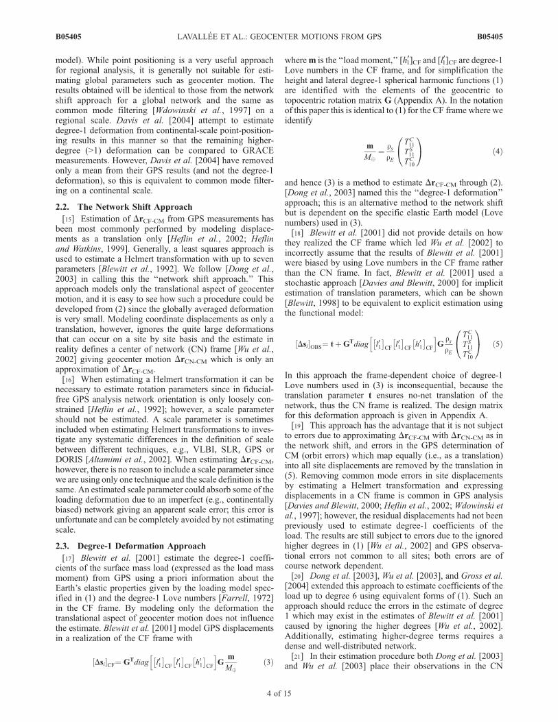
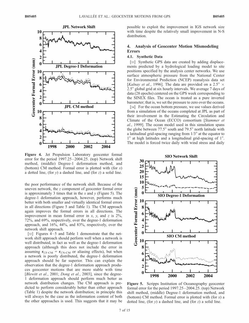
approach in dealing with different networks is reflected inthe similarity between the rCF-CM x, y, and z formal error; ina robust approach the formal error on the geocenter will bethe same in all directions whatever the network distribution.[30] Figure 4 shows the formal error in the JPL geocenter
x, y, and z components from each of the three methods forthis interval. The formal error in all approaches reduces withtime; this to some degree reflects improvements in GPSsoftware models, but mostly reflects the increase in size ofthe GPS tracking network (Figure 2) which is about 100%over the entire interval. The distribution of the network(Figure 3) remains relatively well balanced and consistentover time and this is reflected in the formal errors for thenetwork shift approach being roughly identical in x, y, and zdirections (Figure 4 and Table 1). The network shift methodis predicted to perform slightly better than the degree-1deformation approach for all components. In part, this isdue to dilution of precision: It is necessary to estimatethree extra parameters in the degree-1 deformation ap-proach. Of most interest is that the CM approach ispredicted to give mean formal errors between 42–52%smaller than either the network shift or degree-1 defor-mation approaches.[31] Figure 5 shows the formal error in the SIO geocenter
x, y, and z components from each of the three methods forthe same interval. The results are quite different to those ofthe JPL network since the SIO network includes more sites(Figures 2 and 3). In this case the most noticeable effect is
Figure 2. Number of sites in each analysis center’s weeklysolution for the period 1997.25–2004.25. Values are givenafter outlier rejection and elimination of sites with less than104 weekly observations or less than 2.5 years of data.
Figure 3. Percentage of all analysis center sites in thehemisphere centered on positive x, y, and z axes for theperiod 1997.25–2004.25. The 50% line represents the idealsituation of a well-distributed network.
B05405 LAVALLEE ET AL.: GEOCENTER MOTIONS FROM GPS
6 of 15
B05405
the poor performance of the network shift. Because of theuneven network, the z component of geocenter formal erroris approximately 3 times that in the x and y (Figure 5). Thedegree-1 deformation approach, however, performs muchbetter with both smaller and virtually identical formal errorsin all directions (Figure 5 and Table 1). The CM approachagain improves the formal errors in all directions. Theimprovement in mean formal error in x, y, and z is 2%,72%, and 69%, respectively, over the degree-1 deformationapproach, and 16%, 44%, and 83%, respectively, over thenetwork shift approach.[32] Figures 4–5 and Table 1 demonstrate that the net-
work shift approach should perform well when a network iswell distributed, in fact as well as the degree-1 deformationapproach (although this does not include the error inassuming rCF-CM = rCN-CM or aliasing effects), but whena network is poorly distributed, the degree-1 deformationapproach should be far superior. This can explain theobservation that the degree-1 deformation approach produ-ces geocenter motions that are more stable with time[Blewitt et al., 2001; Dong et al., 2003], since the degree-1 deformation approach should perform much better asnetwork distribution changes. The CM approach is pre-dicted to perform considerably better than either approach(Table 1) despite the network distribution; in principle thiswill always be the case as the information content of boththe other approaches is used. This suggests that it may be
possible to exploit the improvement in IGS network sizewith time despite the relatively small improvement in N-Sdistribution.
4. Analysis of Geocenter Motion MismodelingErrors
4.1. Synthetic Data
[33] Synthetic GPS data are created by adding displace-ments predicted by a hydrological loading model to sitepositions specified by the analysis center networks. We usesurface atmospheric pressure from the National Centerfor Environmental Prediction (NCEP) reanalysis data set[Kalnay et al., 1996]. The data are provided on a 2.5� �2.5� global grid at six hourly intervals. We average 7 days ofdata (28 epochs) centered on the GPS week corresponding tothe SINEX files. The ocean is treated as a pure invertedbarometer; that is, we set the pressure to zero over the oceans.[34] For the ocean bottom pressure, we use values derived
from a simulation of the oceans completed at JPL as part oftheir involvement in the Estimating the Circulation andClimate of the Ocean (ECCO) consortium [Stammer etal., 1999]. The ocean model used in this simulation spansthe globe between 77.5� south and 79.5� north latitude witha latitudinal grid-spacing ranging from 1/3� at the equator to1� at high latitudes and a longitudinal grid-spacing of 1�.The model is forced twice daily with wind stress and daily
Figure 4. Jet Propulsion Laboratory geocenter formalerror for the period 1997.25–2004.25. (top) Network shiftmethod, (middle) Degree-1 deformation method, and(bottom) CM method. Formal error is plotted with (for x)a dotted line, (for y) a dashed line, and (for z) a solid line.
Figure 5. Scripps Institution of Oceanography geocenterformal error for the period 1997.25–2004.25. (top) Networkshift method, (middle) Degree-1 deformation method, and(bottom) CM method. Formal error is plotted with (for x) adotted line, (for y) a dashed line, and (for z) a solid line.
B05405 LAVALLEE ET AL.: GEOCENTER MOTIONS FROM GPS
7 of 15
B05405
surface heat flux and evaporation-precipitation fields fromthe NCEP/NCAR reanalysis project. The 12 hourly datawere averaged into weekly values.[35] We use continental water storage variations derived
from simulations of global continental water and energybalances, created by forcing the LandDynamics (LaD)model[Shmakin et al., 2002] with estimated atmospheric variables.The water storage data (snow, groundwater, and soil mois-ture) are provided at 1��1� global resolution at monthly timeperiods. The most recent version of the model, LaD World-Danube, extends from January 1980 to April 2004. Themonthly data were linearly interpolated to weekly values.[36] The total load is made gravitationally self-consistent
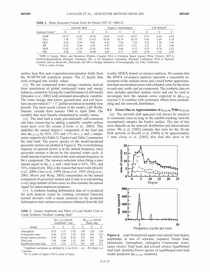
and mass conserving by adding a spatially variable surfacemass layer over the oceans [Clarke et al., 2005]. Thisamplifies the annual degree-1 component of the load andalso DrCF-CM by 26%, 13% and 17% in x, y, and z compo-nents, respectively (Table 2). Figure 6 and Table 2 summarizethe total load. The power spectra of the model-predictedgeocenter motion are plotted in Figure 6. The overwhelmingmajority of spectral power is at the annual frequency sincegeocenter motion is driven by the seasonal water cycle. Asmall amount of power exists at the semi-annual frequency inthe z component. The variance reduction when fitting a pureannual signal to the x, y, and z total load is 65%, 70%, and53%, respectively. This is the reason that most work [Bouilleet al., 2000; Chen et al., 1999;Dong et al., 1997;Dong et al.,2003; Moore and Wang, 2003] concentrates on the annualcomponent of geocenter motion and if only to avoid plottinga very large number of time series we also consider the annualsignal for intercomparison purposes.[37] A synthetic loading deformation data set is produced
for each analysis center by creating correlated Gaussiannormal deviates with a mean centered on the predicteddeformation and variance-covariances obtained from the full
weekly SINEX formal covariance matrices. We assume thatthe SINEX covariance matrices represent a reasonable as-sessment of the random errors and a much better approxima-tion than uncorrelated errors with a blanket value for the noisein each east, north, and up component. The synthetic data setnow includes specified random errors and can be used toinvestigate how the random errors expected in DrCF-CM(section 3.3) combine with systematic effects from mismod-eling and site network distribution.
4.2. Errors Due to Approximation of rCF-CM With rCN-CM[38] The network shift approach will always be sensitive
to systematic error so long as the satellite-tracking networkincompletely samples the Earth’s surface. The size of thiserror depends on the network distribution and observationalerrors: Wu et al. [2002] estimate this error for the 30-siteSLR network of Bouille et al. [2000] to be approximately1 mm; Dong et al. [2002] also find this error to be
Table 1. Mean Geocenter Formal Error for Period 1997.25–2004.25
Analysis CenteraNetwork Shift Degree-1 Deformation CM Methodb
aEMR is Energy, Mines, and Resources (Ottawa, Canada); ESA is European Space Agency (Paris, France); GFZ isGeoForschugsZentrum (Potsdam, Germany); JPL is Jet Propulsion Laboratory (Pasdena, California); NGS is NationalGeodetic Survey (Rockville, Maryland); and SIO is Scripps Institution of Oceanography (La Jolla, California).
bCM is center of mass.
Table 2. Annual Amplitude and Phase of Load Model Used to
aAmplitude and phase are defined by A cos [2p(t t0) F] where t0 is1 January.
bCF is center of figure; CM is center of mass.
Figure 6. (top) Normalized square root annual load degreeamplitudes in mm of seawater. (squares) Ocean load;(diamonds) Atmosphere; (triangles) Continental water;(open circles) Total load; and (closed circles) Equilibratedtotal load. (bottom) Power spectra of equilibrated total loadmodel predicted DrCF-CM variations.
B05405 LAVALLEE ET AL.: GEOCENTER MOTIONS FROM GPS
8 of 15
B05405
submillimeter. In both cases uncorrelated errors are as-sumed. While 1 mm is still significant when the modeledsignal is on the order of 3–4 mm [Chen et al., 1999; Donget al., 1997; Moore and Wang, 2003], assuming uncorrelat-ed errors is likely to seriously underestimate the error whenestimating the mean site displacement if real correlationsexist. We compute this error for each analysis centernetwork series using correlated synthetic data. The resultsare plotted in Figures 7 and 8 and discussed in section 4.4.
4.3. Errors Due to Higher Degrees of Loading
[39] The degree-1 deformation and CM approaches arenot subject to errors in approximating rCF-CM with rCN-CMsince the deformation is modeled at each site (i.e., in the CNframe); however, only the degree-1 deformation is modeled,and degrees >1 are ignored. Ignoring these higher degreescould cause significant aliasing into the estimated geocentermotion [Wu et al., 2002]. Wu et al. [2002] conduct asensitivity analysis to estimate geocenter motion annualamplitude and consider uncertainties for the 66-site network
of Blewitt et al. [2001] to be (9, 8, 10) and (3, 2, 9) mm in x,y, and z, respectively, for two different load scenarios. Wu etal. [2002] scaled the degrees 2 to 50 coefficients in theirload scenarios by 6.6, the load moment z component ofBlewitt et al. [2001]. Wu et al. [2002] may have over-estimated the effects of aliasing with such a scaling,especially since the load moment results of Blewitt et al.[2001] were likely already aliased.[40] We compute the aliasing error for each analysis
center network series, the degree-1 deformation and CMapproaches using the correlated synthetic data. The resultsare plotted in Figures 7 and 8 and discussed in section 4.4.
4.4. Results
[41] Estimates of the two mismodeling errors discussed insections 4.2 and 4.3 are plotted alongside each other inFigures 7 and 8; values estimated from the synthetic datasets are compared with the ‘‘true’’ values used to create thedata. This way the systematic errors introduced in thenetwork shift approach by approximation of CF with CNcan be contrasted with the systematic errors introduced inthe degree-1 deformation and CM approaches by higher-degree aliasing. Observational random errors (section 3.3)
Figure 7. Histogram of DrCF-CM annual amplitudedifferences (mm) between those estimated from syntheticdata and true value used to create the data. Shaded barsindicate that in addition to degree-1 deformation, degree-2deformations were also estimated. Error bars are 1 standarddeviation.
Figure 8. Histogram of DrCF-CM annual phase differences(degrees) between those estimated from synthetic data andtrue value used to create the data. Dotted bars indicate thatin addition to degree-1 deformation, degree-2 deformationswere also estimated. Error bars are 1 standard deviation.
B05405 LAVALLEE ET AL.: GEOCENTER MOTIONS FROM GPS
9 of 15
B05405
are the same for all methods as they are specified by thesynthetic data.[42] Previous work with uncorrelated synthetic data
[Dong et al., 2002; Wu et al., 2002] suggests that annualmismodeling errors are on the order of �1 mm for thenetwork shift approach and up to �6 mm in the degree-1deformation approach; similar results have been obtainedwith uncorrelated data by the authors of this paper. Suchresults can, however, be misleading, since global GPSsolutions will have correlated random errors. If we look atour synthetic data set where intersite correlations are con-sidered (Figures 7 and 8), a very different picture emerges;in this case, network shift annual amplitude can vary fromthe true value by as much as �4 mm in x and y, up to 10 mmin z, and between analysis centers by almost as much. Thephase variations are even more extreme with some phasesshifted almost 180� from both the true value and betweenanalysis centers. These results indicate that correlated errorsin global geodetic solutions could cause significant errorsand disagreement between estimates of geocenter motionwhen using the network shift approach (particularly whenusing different networks); this error is much larger thanaliasing effects in the deformation approach. This conclu-sion is enhanced by the poor agreement between GPSgeocenter motion estimates using the network shift ap-proach [Boucher and Sillard, 1999] and observations thatthe degree-1 deformation approach produces more stableresults [Dong et al., 2003].[43] The degree-1 deformation method produces better
results than the network shift approach (Figures 7 and 8),with annual amplitudes that are generally closer to the truevalue and in better agreement between different networks(particularly in z). The improvement in phase stability isquite considerable. Aliasing of higher degrees still has aneffect, and the best degree-1 deformation results areachieved when degree 2 is also estimated; in this case,errors are up to 0.8, 0.9, and 2.6 mm in x, y, and zamplitudes, respectively; in phase, errors are up to 31�,42�, and 26�, respectively.[44] The CM method consistently produces results which
are closer to the true value than are either the network shiftor degree-1 deformation approaches (Figures 7 and 8).When degree 2 is also estimated, amplitude errors arepredicted to be up to 0.5, 0.3, and 2.5 mm in x, y, and z,respectively; if the network is well distributed, then the errorin z can be as low as 0.6 mm. Phase errors are predicted tobe up to 22�, 26� and 28� in x, y, and z, respectively. Themethod is in principle the best way to model the observa-tions and from this simulated analysis is indeed the bestperformer.[45] It can be observed that for all methods the SIO
network produces results in amplitude and phase that areusually furthest from the true value, particularly whendegree 2 is not estimated. This network contains a largenumber of regional sites and demonstrates the effects of avery uneven network. It is unlikely that such sites wouldnormally be included in a geocenter estimation analysis;however, inclusion of these sites provides a useful end-member estimate of the errors. For such a large network it ispossible to estimate spherical harmonic degrees greater than2 with the deformation approaches [Wu et al., 2003]. Onlythe SIO network is really large enough to do this reliably
(Figure 2). We estimate up to degree 6 with the degree-1deformation approach and CM approach from the syntheticdata; in this case, we find that the annual x and y amplitudesdo not get any closer to their true values compared to thecase when only degrees 1 and 2 were estimated, but the SIOz amplitudes now vary from the true value by only 0.4 mm,an improvement of 84%, with the annual phase hardlyaffected. This suggests that, while aliasing from degreesbeyond 2 is minimal for x and y, the tendency for an unevennetwork in the z direction requires higher degrees to beestimated to overcome aliasing and that this may be a viableapproach for large but regionally dense networks such asSIO.
5. Network Scale
[46] It is common when estimating Helmert transforma-tions to estimate a scale parameter [Heflin et al., 2002]. Inthe case of an uneven network this scale parameter couldabsorb some of the real deformation due to surface massloading and is unnecessary when geocenter motions areestimated. This effect has been found significant forthe network shift approach with noise-free, uncorrelatedsynthetic site data from just atmospheric pressure loading[Tregoning and van Dam, 2005]. The effect on the esti-mated DrCF-CM of including a scale parameter is inves-tigated here, for correlated and noisy synthetic data from theentire surface load and additionally real GPS data.[47] With the synthetic data, estimating scale has the
largest effect on DrCF-CM estimated using the network shiftapproach. This effect is very significant in the z component;the annual amplitude is altered by up to 0.33, 0.16, and1.5 mm in x, y, and z components, respectively. When usingeither of the deformation approaches the z componentchanges only up to 0.4 mm, phase differences are at most3� for x and y with a network shift z value of 10�.[48] For the real data the picture is very similar: The
effect on the estimated DrCF-CM is significant with amaximum effect on annual amplitude of 1.29 mm in x,2.11 mm in y, and 4.6 mm in z. These differences are againmaximal for the network shift approach; for the unifiedapproach the maximum effect is 0.86, 0.81, and 3.23 mm inz. The effect on annual phase can reach 68� in x with thenetwork shift method.[49] The size of the estimated scale parameter is also
significant. In the synthetic data, there is no true scalevariation, only scale error arising through the interactionbetween loading and network geometry. Figure 9 plots thepower spectra of the scale series estimated for each method(network shift, degree-1 deformation, etc.), averaged overall analysis centers. The averaging is simply for clarity; thesame observations are made from each individual analysiscenter scale spectrum. In the synthetic data (Figure 9a) thescale series power spectrum is flat with a sharp peak at theannual frequency; this is largest (and significant at 5%) forthe network shift approach and gets progressively smaller(and no longer significant) when using the degree-1 defor-mation and CM approaches. If degree 2 is included in theselatter methods then it gets smaller still. Figure 9b also plotsthe power spectra of the scale estimated from the real data;there is a clear annual peak which is largest for the networkshift approach and reduces in amplitude when increasing
B05405 LAVALLEE ET AL.: GEOCENTER MOTIONS FROM GPS
10 of 15
B05405
amounts of the loading deformation are estimated. Themean amplitude of seasonal scale estimated from thenetwork shift approach is 0.15 ppb for the synthetic dataand 0.37 ppb for the real data. It is likely that the observedseasonal changes in scale of 0.37 ppb and other results onthe order of 0.3 ppb [Heflin et al., 2002] are due to aliasingof the loading signal. It is encouraging to realize that theseasonal signals observed in GPS scale are at least partlydue to a real loading signal rather than any particular GPSspecific systematic error.[50] Another possible scale error exists when results are
put in the CN frame using a seven parameter Helmerttransformation and then the residuals are used to estimatethe deformation due to surface loading with the degree-1deformation approach [Dong et al., 2003; Wu et al., 2003].In this scenario it is possible that the estimation andsubsequent removal from the data of a scale parametercould also remove some actual deformation due to loading.We estimate the size of the error in geocenter motionsestimated this way from the synthetic data to be up to1.84 mm in annual amplitude and up to 40� in phase. Withthe real data, using such a two-step procedure can changethe estimates by as much as 4.3 mm in annual amplitudeand 85� in phase. The effect of this two-step approach isgenerally to reduce load amplitude since some of the poweris absorbed by the scale parameter; It is likely that this
accounts for the significant reduction in annual degree-1amplitude observed by Dong et al. [2003] compared toBlewitt et al. [2001].
6. Comparison of Estimated Geocenter Motion
[51] Geocenter motions for the period 1997.25–2004.25are estimated from the GPS solutions for each of the six IGSanalysis centers. Annual amplitude and phase are shown inFigures 10 and 11; for comparison the predicted values fromthe loading model are also given. Comparing these solutionsgives insight into both network and modeling effects; eachanalysis center has used the same GPS data but sometimesvery different networks, analysis software, and procedures.The most noticeable result of this analysis is the largedisagreement between analysis centers in geocenter motionannual phase for the network shift approach z component(Figure 11), this can be as large as 166� and apart from onecomparison is always greater than 50�. Such a situation is
Figure 9. Average power spectra of estimated scale (a) forsynthetic GPS data and (b) for real GPS data. Scaleestimated with (topmost solid line) network shift approach,(dotted line) degree-1 deformation, and (dashed line) theCM method. Two lowermost solid lines in both plots are thedegree-1 and CM deformation approaches where degree 2 isalso estimated. Horizontal dash-dotted line in Figure 9a is5% significance level assuming background white noisewith a variance estimated from background spectra.
Figure 10. Histogram of GPS-estimated DrCF-CM annualamplitude (mm). Shaded bars indicate that in addition todegree-1 deformation, degree-2 deformations were alsoestimated. Error bars are 1 standard deviation. Solidhorizontal lines are mean satellite laser ranging (SLR)estimates discussed in text. Dotted horizontal lines areequilibrated load model predicted values of DrCF-CM annualamplitude.
B05405 LAVALLEE ET AL.: GEOCENTER MOTIONS FROM GPS
11 of 15
B05405
predicted by the simulated data (section 4.4, Figure 8) andresults from a very uneven network in the z direction. Thisresult combined with that from the synthetic analysis clearlyexplains the disagreement previously seen amongst GPSestimated geocenter motions using the network shift ap-proach [Boucher and Sillard, 1999]. Furthermore it suggestsserious shortcomings in the network shift approach forestimating geocenter motions from GPS. In addition tonetwork effects one possible explanation is the differentstrategies taken to ambiguity fixing; however, only JPLresolves all ambiguities; the other analysis centers fix someor none at all and no consistent differences are observed inFigures 10 and 11.[52] The two deformation methods give considerably
better agreement in phase (Figure 11); in fact, the estimatesof annual phase from these methods appear to be much lessaffected by aliasing, network size, and distribution than isthe estimated annual amplitude, another result predicted bythe simulated data analysis. The weighted root- mean-square (WRMS) annual phase values (about the weightedmean) are around 15� in all components for the CM and
Figure 11. Histogram of estimated DrCF-CM annual phase(degrees). Dotted outline bars indicate that in addition todegree-1 deformation, degree-2 deformations were alsoestimated. Error bars are 1 standard deviation. Solidhorizontal lines are mean SLR estimates discussed in text.Dotted horizontal lines are equilibrated load modelpredicted values of DrCF-CM annual phase.
Table 3. Mean and Weighted RMS Estimated Analysis Center
DrCF-CM Annual Amplitude and Phase for Period 1997.25–
aAmplitude and phase are defined by A cos [2p(t t0) F] where t0 is 1January. CF is center of figure; CM is center of mass. SIO is ScrippsInstitution of Oceanography.
B05405 LAVALLEE ET AL.: GEOCENTER MOTIONS FROM GPS
12 of 15
B05405
degree-1 deformation methods compared with 15�, 17� and108� in x, y, and z for the network shift method (Table 3).[53] In Figure 10 the solution for ESA is in disagreement
with the other analysis centers for all approaches; the reasonfor this is unknown. If we treat this solution as an outlier andexclude it, then annual amplitude agreement between theremaining five analysis center solutions is much improved(Table 3).[54] The deformation methods are affected by aliasing. If
degree 2 is also estimated then the deformation methodsperform much better in amplitude as predicted by thesimulated results, particularly for the large network SIO(Figure 10). The SIO network is very unevenly distributed,not normally a choice for estimating geocenter motions ordefining a frame. If we restrict ourselves to ‘‘reasonable’’networks only (the remaining four analyses), then thenetwork shift method gives WRMS amplitude variation ofaround 1.5 mm and the degree-1 plus degree-2 method has alarger z agreement, but by far the best performance isachieved when using the CM + 2 approach: WRMSvariation is entirely submillimeter at 0.6, 0.6, and 0.3 mmin x, y, and z (Table 3). In this context ‘‘reasonable’’ meansthat clustering in one axis-centered hemisphere is limited toless than 70% of sites (Figure 3).[55] The simulated analysis (section 4.4) and Wu et al.
[2003] suggest that estimating additional higher degrees ofthe load may overcome the problems of an uneven network.We estimate degrees 1 through 6 for the SIO network. Inthis case, the WRMS variation in x, y, and z amplitude is0.6, 0.6, and 0.8 mm for the CM approach (Table 3). Theseresults suggest that estimating higher degrees in the CMframe is a valid approach to take for large unevenlydistributed networks; it performs almost as well as whenusing evenly distributed networks and just estimatingdegrees 1 and 2. Table 3 also suggests that modelinghigher-degree deformations in the CM rather than CN framegives improved results. Removing higher-degree deforma-tions using GRACE results [Davis et al., 2004] is anotherapproach that may improve geocenter estimates; however,this would not be possible prior to 2002. In section 2.1 itwas stated that the CM method reduces to the network shiftmethod in the case of a diagonal or block diagonal weightmatrix. This is easily verified and has been done for theresults presented here; the CM and network shift methodsproduce near identical results in this case.[56] The estimated annual amplitude and phase are com-
pared with those predicted by the load model (section 4.1).Horizontal dotted lines representing the load model valuesare included in Figures 10 and 11, and the mean estimatedvalues in Table 3 can be compared with the loading modelpredicted values in Table 2. In this comparison the CMmethod where degree 2 is also estimated is in best agree-ment with the loading model; consistently, the annualamplitude and phase are closer to that predicted by theloading model than any other method, whether SIO isincluded or not (still treating ESA as an outlier). ExcludingSIO and ESA, agreement of the weighted mean annualamplitude with the load model is 0.09, 0.95, and 0.91 mm.If degrees up to 6 are estimated from SIO then the results areonly slightly different (Table 3). Phase differences with theload model are 14�, 3�, and 35� in x, y, and z, respectively.These difference are much larger than our formal errors
(Table 3); however, if only because of aliasing, the formalerrors are obviously too small. An improved estimate of theobservational errors comes from the WRMS agreementbetween the analysis center values (Table 3). In this casethe load model falls within 2 standard deviations of the CMapproach best estimate (mean of four analysis centers).[57] The annual amplitude and phase are also compared
to network shift results from SLR tracking of LAGEOS 1and 2 [Bouille et al., 2000; Chen et al., 1999; Cretaux et al.,2002; Moore and Wang, 2003]. The four SLR results are invery good agreement with a mean annual amplitude of 2.60,3.00, and 3.55 mm, mean phase of 221�, 130�, and 219�,RMS amplitude of 0.56, 0.86, and 0.66 mm, and RMSphase of 13�, 11�, and 5� in x, y, and z, respectively.Compared to the best estimates from GPS using the CM+ 2 approach (Table 3) SLR has near identical annualamplitude RMS but half that achieved by GPS in annualphase RMS. It is clear that the SLR results do not have thesame errors in the network shift as GPS; the improvedsensitivity of LAGEOS 1 and 2 to the geocenter means thecombination of observational and approximation errors (CFwith CN) are smaller. The systematic error from approxi-mating CF with CN still exists, however, and, since the SLRtracking network does not vary to the degree GPS does, islikely similar between estimates. The CM approach couldimprove SLR geocenter estimates still further.[58] The mean SLR result is plotted on Figures 10 and 11,
differences between the mean SLR estimate, the best GPSmean estimate (CM + 2) and the loading model areinsignificant at 2 sigma when the RMS is used as anestimate of formal error. At the 1 sigma level, there is asignificant discrepancy between the geodetic measurements(which agree) and the load model in z amplitude, and the yannual phase from SLR is significantly different from bothGPS and the load model.[59] The considerably improved precision of the CM
approach is still not small enough to reliably discriminatebetween different load models; however, the level of agree-ment between geodetic estimates of geocenter annual mo-tion (Table 3) is now about the same level as that betweendifferent load models, a considerable improvement in ob-servational precision over that previously seen from GPS.
7. Conclusions
[60] Historically, the ‘‘network shift’’ approach has been themost commonly used approach to estimating geocentermotions from geodetic data. We find that it has a number ofshortcomings when applied to GPS. Estimated and predictedresults from synthetic data demonstrate that the geocenterannual phase estimated by the network shift is particularlyunstable. Significant levels of seasonal scale variation ob-served in GPS analysis are at least in part due to the interactionof surface mass loading with a sparse geodetic network andmismodeling of the Earth’s degree-1 deformations with thenetwork shift approach. Scale should not be estimated withgeocenter motions, or biased results will be obtained.[61] Alternative approaches for estimating geocenter
motions with GPS have involved modeling the degree-1(and sometimes higher) deformations in realizations of theCF frame [Blewitt et al., 2001; Dong et al., 2003; Wu et al.,2003]. In terms of formal error, modeling the deformations
B05405 LAVALLEE ET AL.: GEOCENTER MOTIONS FROM GPS
13 of 15
B05405
in this way is much more robust when networks are uneven.Aliasing from unestimated higher degrees, although impor-tant, can be alleviated by estimating the total load to degree2, but in the case of very large unevenly distributed net-works even higher degrees must be estimated.[62] In principle, an approach that unifies both the trans-
lation and deformation aspects of geocenter motion is morecomplete, should take advantage of all GPS informationcontent, and is conventional since all deformations aremodeled in the CM frame. Such an approach is found togive the lowest geocenter motion formal error, smallerdifferences from the true value when using synthetic data,the best agreement between five different GPS analyses andthe closest agreement with the geocenter motion predictedfrom loading models and estimated from SLR.[63] A note of caution must be attached, however: Unless
the unified (CM) method uses a full weight matrix that isobtained from simultaneous estimation of station coordi-nates with orbit parameters, the relative weight of informa-tion between the translation and deformation would beincorrect. For example, using the covariance matrix fromprecise point positioning (which fixes the orbits) would beinappropriate and would produce nearly identical, poorerresults to the network shift approach.[64] With this newest approach, provided care is taken to
ensure a balanced network or higher degrees are estimatedas required, we demonstrate that it is possible to estimategeocenter motions from GPS with unprecedented submilli-meter levels of precision. This level of precision is still,however, insufficient to reliably discriminate between dif-ferent loading models. Geocenter motion agreement be-tween different GPS solutions is now at the same level asgeocenter motion agreement between different loadingmodels. With improved GPS error modeling and mitigation,reprocessing of older data and further placement of GPSsites in the Southern Hemisphere, a level of precision thatcan in the near future discriminate between load modelsdoes now appear possible.
Appendix A: Least Squares Design Matrices
A1. CM Approach
[65] Displacements are modeled completely in the CMframe using (1) and Love numbers in the CM frame. Theparameter vector is
x ¼ rx ry rzj
j
j
j
j
DrCFCM
j
j
j
j
j
TC22 TS
22 TC21 TS
21 TC20 � � �TC
�n0
� �T
ðA1Þwhere rx, ry, and rz are rotation parameters, DrCF-CM is thegeocenter motion, and Tnm
F are spherical harmonic coeffi-cients of the higher degrees (>1) of the total surface load.The choice to include higher degrees is optional. The leastsquares design matrix for the ith site is
Ai ¼0 z y
z 0 x
y x 0
j
j
j
j
j
j
j
j
j
3
h01� �
CEþ2 l01
� �CE
� � 1
0@
1A
0B@
�GTi diag l01
� �CM
l01� �
CMh01� �
CM
h iGi
j
j
j
j
j
j
j
j
j
Bi
!ðA2Þ
where Gi is the 3 � 3 matrix that rotates geocentric intotopocentric displacements (east, north, and up) about a pointwith latitude j and longitude l.
Gi ¼ sinl cosl 0
sinj cosl sinj sinl cosjcosj cosl cosj sinl sinj
0@
1A ðA3Þ
The matrix Bi contains the partial derivatives for higherdegrees (>1) from (1).
A2. Network Shift Approach
[66] Generally, a least squares approach is used to esti-mate a Helmert transformation with up to seven parameters
x ¼ tx ty tzj
j
j
j
j
sj
j
j
j
j
rx ry rz� �T
ðA4Þ
where the parameter t = (tx ty tz)T is the least squares
estimate of DrCF-CM and s is an optional scale parameter;the design matrix is
Ai ¼1 0 0
0 1 0
0 0 1
j
j
j
j
j
j
j
j
j
xiyizi
j
j
j
j
j
j
j
j
j
0 zi yizi 0 xiyi xi 0
0@
1A ðA5Þ
A3. Degree-1 Deformation Approach
[67] In the degree-1 deformation approach the parametervector is
x ¼ txtytzj
j
j
j
j
rxryrzj
j
j
j
j
rCFCM
j
j
j
j
j
TC22T
S22T
C21T
S21T
C20� � �TC
�n0
� �T
ðA6Þ
With translation t and rotation r (which are both discarded),geocenter motion DrCF-CM and higher degrees up to degreen of the surface mass load, the design matrix is
Ai ¼1 0 0
0 1 0
0 0 1
j
j
j
j
j
j
j
j
j
0 z y
z 0 x
y x 0
j
j
j
j
j
j
j
j
j
0B@ 3
h01� �
CEþ2 l01
� �CE
� � 1
0@
1A
�GTi diag l01
� �CF
l01� �
CFh01� �
CF
h iGi
j
j
j
j
j
j
j
j
j
Bi
!ðA7Þ
[68] Acknowledgments. We thank the IGS analysis centers for pro-viding the SINEX solutions used in this work. We would like to thankYehuda Bock, Erricos Pavlis, and Mike Watkins for constructive reviews.The authors acknowledge a Royal Society University Research Fellowshipto DAL and funds from the Luxembourg government for a visit of DAL tothe European Center for Geodynamics and Seismology, April –May 2004.This work was also supported in the UK by NERC grant NER/A/S/2001/01166 to PJC and in the USA by NASA Solid Earth and Natural Hazardsgrant SENH-0225-0008 to GB.
ReferencesAltamimi, Z., P. Sillard, and C. Boucher (2002), ITRF2000: A new releaseof the International Terrestrial Reference Frame for Earth science appli-cations, J. Geophys. Res., 107(B10), 2214, doi:10.1029/2001JB000561.
Argus, D. F., W. R. Peltier, and M. M. Watkins (1999), Glacial isostaticadjustment observed using very long baseline interferometry and satellitelaser ranging geodesy, J. Geophys. Res., 104(B12), 29,077–29,093.
B05405 LAVALLEE ET AL.: GEOCENTER MOTIONS FROM GPS
14 of 15
B05405
Blewitt, G. (1998), GPS data processing methodology: From theory toapplications, in GPS for Geodesy, edited by P. J. G. Teunissen andA. Kleusberg, pp. 231–270, Springer, New York.
Blewitt, G. (2003), Self-consistency in reference frames, geocenter defini-tion, and surface loading of the solid Earth, J. Geophys. Res., 108(B2),2103, doi:10.1029/2002JB002082.
Blewitt, G., and P. Clarke (2003), Inversion of Earth’s changing shape toweigh sea level in static equilibrium with surface mass redistribution,J. Geophys. Res., 108(B6), 2311, doi:10.1029/2002JB002290.
Blewitt, G., and D. Lavallee (2002), Effect of annual signals on geodeticvelocity, J. Geophys. Res., 107(B7), 2145, doi:10.1029/2001JB000570.
Blewitt, G.,M.B.Heflin, F.H.Webb,U. J. Lindqwister, andR. P.Malla (1992),Global coordinates with centimeter accuracy in the International TerrestrialReference Frame using GPS, Geophys. Res. Lett., 19(9), 853–856.
Blewitt, G., Y. Bock, and J. Kouba (1995), Constructing the IGS polyhe-dron by distributed processing, in Densification of the IERS TerrestrialReference Frame Through Regional GPS Networks, edited by J. F.Zumberge and R. Liu, pp. 21–38, Int. GPS Serv., Pasadena, Calif.
Blewitt, G., D. Lavallee, P. Clarke, and K. Nurutdinov (2001), A newglobal mode of Earth deformation: Seasonal cycle detected, Science,294(5550), 2342–2345.
Boucher, C., and P. Sillard (1999), Synthesis of submitted geocenter timeseries, in IERS Analysis Campaign to Investigate Motions of the Geocen-ter, IERS Tech. Note 25, pp. 15–21, Obs. de Paris, Paris.
Bouille, F., A. Cazenave, J. M. Lemoine, and J. F. Cretaux (2000), Geo-centre motion from the DORIS space system and laser data to theLAGEOS satellites: Comparison with surface loading data, Geophys.J. Int., 143(1), 71–82.
Chen, J. L., C. R. Wilson, R. J. Eanes, and R. S. Nerem (1999), Geophy-sical interpretation of observed geocenter variations, J. Geophys. Res.,104(B2), 2683–2690.
Cheng, M. K. (1999), Geocenter variations from analysis of TOPEX/POEIDON SLR data, in IERS Analysis Campaign to Investigate Motionsof the Geocenter, IERS Tech. Note 25, pp. 39–44, Obs. de Paris, Paris.
Clarke, P. J., D. Lavallee, G. Blewitt, T. van Dam, and J. M. Wahr (2000),Effect of gravitational consistency and mass conservation on seasonalsurface mass loading models, Geophys. Res. Lett., 32, L08306,doi:10.1029/2005GL022441.
Cretaux, J. F., L. Soudarin, F. J. M. Davidson, M. C. Gennero, M. Berge-Nguyen, and A. Cazenave (2002), Seasonal and interannual geocenter mo-tion from SLR and DORISmeasurements: Comparison with surface loadingdata, J. Geophys. Res., 107(B12), 2374, doi:10.1029/2002JB001820.
Davies, P., and G. Blewitt (2000), Methodology for global geodetic timeseries estimation: A new tool for geodynamics, J. Geophys. Res.,105(B5), 11,083–11,100.
Davis, J. L., P. Elosegui, J. X. Mitrovica, and M. E. Tamisiea (2004),Climate-driven deformation of the solid Earth from GRACE and GPS,Geophys. Res. Lett., 31, L24605, doi:10.1029/2004GL021435.
Diziewonski, A., and D. L. Anderson (1981), Preliminary reference Earthmodel, Phys. Earth Planet. Inter., 25, 297–356.
Dong, D., J. O. Dickey, Y. Chao, and M. K. Cheng (1997), Geocentervariations caused by atmosphere, ocean and surface groundwater, Geo-phys. Res. Lett., 24(15), 1867–1870.
Dong, D., P. Fang, Y. Bock, M. K. Cheng, and S. Miyazaki (2002), Anat-omy of apparent seasonal variations from GPS-derived site position timeseries, J. Geophys. Res., 107(B4), 2075, doi:10.1029/2001JB000573.
Dong, D., T. Yunck, and M. Heflin (2003), Origin of the International Ter-restrial Reference Frame, J. Geophys. Res., 108(B4), 2200, doi:10.1029/2002JB002035.
Farrell, W. E. (1972), Deformation of the Earth by surface loads, Rev.Geophys., 10, 761–797.
Gross, R. S., G. Blewitt, P. J. Clarke, and D. Lavallee (2004), Degree-2harmonics of the Earth’s mass load estimated from GPS and Earth rota-tion data, Geophys. Res. Lett., 31, L07601, doi:10.1029/2004GL019589.
Heflin, M., and M. Watkins (1999), Geocenter estimates from the GlobalPositioning System, in IERS Analysis Campaign to Investigate Motionsof the Geocenter, IERS Tech. Note 25, pp. 55–70, Obs. de Paris, Paris.
Heflin, M., et al. (1992), Global geodesy using GPS without fiducial sites,Geophys. Res. Lett., 19, 131–134.
Heflin, M., D. F. Argus, D. C. Jefferson, F. H. Webb, and J. F. Zumberge(2002), Comparison of a GPS-defined global reference frame withITRF2000, GPS Solutions, 6, 72–75.
Kalnay, E., et al. (1996), The NCEP/NCAR 40-year reanalysis project, Bull.Am. Meteorol. Soc., 77(3), 437–471.
Kedar, S., G. A. Hajj, B. D. Wilson, and M. B. Heflin (2003), The effect ofthe second order GPS ionospheric correction on receiver positions, Geo-phys. Res. Lett., 30(16), 1829, doi:10.1029/2003GL017639.
Lambeck, K. (1980), Geophysical Geodesy; The Slow Deformations of theEarth, Oxford Univ. Press, New York.
Lavallee, D. (2000), Tectonic plate motions from global GPS measure-ments, Ph.D. thesis, Univ. of Newcastle upon Tyne, Newcastle, U. K.
Lavallee, D., and G. Blewitt (2002), Degree-1 Earth deformation from verylong baseline interferometry measurements, Geophys. Res. Lett., 29(20),1967, doi:10.1029/2002GL015883.
Malla, R. P., S. C. Wu, and S. M. Lichten (1993), Geocenter location andvariations in the Earth orientation using global positioning system mea-surements, J. Geophys. Res., 98(B3), 4611–4618.
McCarthy, D. D., and G. Petit (2004), IERS Conventions (2003), IERSTech. Note, vol. 32, Verl. Bundesamt Kartogr. Geod., Frankfurt am Main,Germany.
Moore, P., and J. Wang (2003), Geocentre variation from laser tracking ofLAGEOS 1/2 and loading data, Adv. Space Res., 31, 1927–1933.
Pavlis, E. C. (1999), Fortnightly resolution geocenter series: A combinedanalysis of LAGEOS 1 and 2 SLR data (1993–1996), in IERS AnalysisCampaign to Investigate Motions of the Geocenter, IERS Tech. Note 25,pp. 75–84, Obs. de Paris, Paris.
Penna, N. T., and M. P. Stewart (2003), Aliased tidal signatures in contin-uous GPS height time series, Geophys. Res. Lett., 30(23), 2184,doi:10.1029/2003GL018828.
Ray, J. (Ed.) (1999), IERS Analysis Campaign to Investigate Motions of theGeocenter, IERS Tech. Note, vol. 25, Obs. de Paris, Paris.
Ray, J., D. Dong, and Z. Altamimi (2004), IGS reference frames: Status andfuture improvements, GPS Solutions, 8(4), 251 –266, doi:10.1007/s10291-004-0110-x.
Shmakin, A. B., P. C. D. Milly, and K. A. Dunne (2002), Global modelingof land water and energy balances. part III: Interannual variability,J. Hydrometeorol., 3(3), 311–321.
Stammer, D., et al. (1999), The consortium for estimating the circulationand climate of the ocean (ECCO), Rep. 1, Natl. Oceanogr. PartnershipProgram, Washington, D. C.
Tapley, B. D., S. Bettadpur, M. Watkins, and C. Reigber (2004), Thegravity recovery and climate experiment: Mission overview and earlyresults, Geophys. Res. Lett., 31, L09607, doi:10.1029/2004GL019920.
Tregoning, P., and T. van Dam (2005), Effects of atmospheric pressureloading and seven-parameter transformations on estimates of geocentermotion and station heights from space geodetic observations, J. Geophys.Res., 110, B03408, doi:10.1029/2004JB003334.
Trupin, A. S., M. F. Meir, and J. Wahr (1992), Effects of melting glaciers onthe Earth’s rotation and gravitational field: 1965–1984, Geophys. J. Int.,108, 1–15.
Vigue, Y., S. M. Lichten, G. Blewitt, M. B. Heflin, and R. P. Malla (1992),Precise determination of Earth’s center of mass using measurements fromthe global positioning system, Geophys. Res. Lett., 19(14), 1487–1490.
Watkins, M. M., and R. J. Eanes (1993), Long term changes in the Earth’sshape, rotation, and geocenter, Adv. Space Res., 13(11), 251–255.
Watkins, M. M., and R. J. Eanes (1994), Diurnal and semidiurnal variationsin Earth orientation determined from LAGEOS laser ranging, J. Geophys.Res., 99(B9), 18,073–18,079.
Watkins, M. M., and R. J. Eanes (1997), Observations of tidally coherentdiurnal and semidiurnal variations in the geocenter, Geophys. Res. Lett.,24(17), 2231–2234.
Wdowinski, S., Y. Bock, J. Zhang, P. Fang, and J. Genrich (1997), SouthernCalifornia permanent GPS geodetic array: Spatial filtering of daily posi-tions for estimating coseismic and postseismic displacements induced bythe 1992 Landers earthquake, J. Geophys. Res., 102(B8), 18,057–18,070.
Wu, X. P., D. F. Argus, M. B. Heflin, E. R. Ivins, and F. H. Webb (2002),Site distribution and aliasing effects in the inversion for load coefficientsand geocenter motion from GPS data, Geophys. Res. Lett., 29(24), 2210,doi:10.1029/2002GL016324.
Wu, X. P., M. B. Heflin, E. R. Ivins, D. F. Argus, and F. H. Webb (2003),Large-scale global surface mass variations inferred from GPS measure-ments of load-induced deformation, Geophys. Res. Lett., 30(14), 1742,doi:10.1029/2003GL017546.
Zumberge, J. F., M. B. Heflin, D. C. Jefferson, M. M. Watkins, and F. H.Webb (1997), Precise point positioning for the efficient and robust ana-lysis of GPS data from large networks, J. Geophys. Res., 102(B3), 5005–5017.
G. Blewitt, MS 178, 1664 N. Virginia Street, University of Nevada,
Reno, NV 89557-0088, USA. ([email protected])P. J. Clarke and D. A. Lavallee, School of Civil Engineering and
Geosciences, Cassie Building, University of Newcastle upon Tyne,Newcastle, NE1 7RU, UK. ([email protected]; [email protected])T. van Dam, European Center for Geodynamics and Seismology, Rue