85
Master Thesis, Department of Geosciences Geological potential for carbon storage in the Sele High, Åsta Graben and NW Egersund Basin area Daniel Long

Master Thesis, Department of Geosciences
Geological potential for carbon storage in the Sele High, Åsta Graben and NW Egersund Basin area
Daniel Long

Geological potential for carbon storage in the Sele High, Åsta
Graben and NW Egersund Basin area
Daniel Long
Master Thesis in Geosciences
Discipline: Geology
Department of Geosciences
Faculty of Mathematics and Natural Sciences
University of Oslo
2012

© Daniel Long, 2012
This work is published digitally through DUO – Digitale Utgivelser ved UiO
http://www.duo.uio.no
It is also catalogued in BIBSYS (http://www.bibsys.no/english)
All rights reserved. No part of this publication may be reproduced or transmitted, in any form or by any means,
without permission.
CHAPTER: INTRODUCTION
Page | 1
Abstract
The rise of carbon dioxide (CO2) emissions in the Earth’s atmosphere has led to an increased
focus on ways to reduce these emissions. One way of doing this is by using carbon capture
and storage (CCS) technology whereby CO2 is collected or captured at point sources and
then injected into deep geological formations to be stored indefinitely.
The Sele High, Åsta Graben and the NW Egersund Basin were investigated in an attempt to
identify potential reservoirs for storing carbon dioxide and then calculating a storage
capacity. This was done using well analysis and seismic interpretation, and was guided by
the Norwegian Petroleum Directorate’s CO2 Storage Atlas 2012.
After investigation of multiple wells and the structures they intersect, two were identified as
having moderate potential. The storage capacity for wells 17/10-1 and 18/10-1 were
calculated to be 750-850 Mt and 35 Mt respectively. The weakest aspect of both prospects
were their limited extent, which is in contrast to existing CO2 storage operations such as the
Sleipner Project that has a storage capacity of approximately 1-10 Gt of CO2. This will be a
challenge considering the extensive halokinesis throughout the Norwegian-Danish Basin in
particular.
CHAPTER: INTRODUCTION
Page | 2
Acknowledgements
I would like to thank my supervisor Per Aargaard for his guidance and patience.
I would also like to thank Michel Heeremans for his technical support.
A special thanks goes to the Administration team at the Geology Department for all there
help.
I would especially like to thank my family for their love support and encouragement.
Daniel Long
December 2012

CHAPTER: INTRODUCTION
Page | 3
TABLE OF CONTENTS
1. INTRODUCTION 7
1.1 INTRODUCTION 8
2. GEOLOGICAL SETTING 9
2.1 LOCATION AND GEOLOGICAL SETTING OF STUDY AREA 10
2.2 REGIONAL GEOLOGY 11
2.3 LING DEPRESSION 13
2.4 SELE HIGH 14
2.5 EGERSUND BASIN 14
2.6 ÅSTA GRABEN 16
2.7 FISKEBANK SUB-BASIN AND THE NORWEGIAN-DANISH BASIN 16
3. STRATIGRAPHY 18
3.1 RESERVOIR ROCKS 20
3.1.1 Sandnes Formation 21
3.1.2 Bryne Formation 22
3.1.3 Gassum Formation 24
3.1.4 Skagerrak Formation 24
4. THEORETICAL BACKGROUND 26
4.1 GEOLOGICAL STORAGE OF CARBON DIOXIDE (CO2) 27
4.1.1 The need for CO2 storage 27
4.1.2 What is Carbon Capture and Storage (CCS)? 28
4.1.3 How is CO2 stored? 30
4.1.4 Who is storing CO2 and where? 32
4.2 CLASSIFICATION / RANKING SCHEMES USED IN THE CO2 ATLAS 35
5. METHODS AND DATA 36
5.1 DATASET 37
5.1.1 Wells 37
5.1.2 Well log quality checks 48
5.1.3 Well Log Analysis 48
5.2 SEISMIC SURVEYS 51
5.2.1 Seismic Interpretation 53
5.2.2 Seismic-to-well tie 54
5.3 STORAGE CAPACITY CALCULATION 54
6. RESULTS 55

CHAPTER: INTRODUCTION
Page | 4
POTENTIAL STORAGE SITES 56
6.1 56
6.2 18/10-1 PROSPECT 56
Reservoir properties 56
6.2.1 56
6.2.2 Porosity 57
6.2.3 Permeability 58
6.2.4 Net-to-gross ratio 59
6.2.5 Seal and caprock 59
6.2.6 Trap 59
6.2.7 Storage Capacity 61
6.2.8 Enhanced Oil Recovery (EOR) 62
6.3 17/10-1 PROSPECT 62
6.3.1 Porosity 64
6.3.2 Permeability 64
6.3.3 Net-to-gross ratio 64
6.3.4 Seal and caprock 65
6.3.5 Trap 65
6.3.6 Storage Capacity 68
7. DISCUSSION 72
7.1 DISCUSSION 73
7.2 LIMITATIONS OF THIS STUDY 73
7.3 SALT STRUCTURES 73
8. CONCLUSION 75
9. REFERENCES 79
CHAPTER: INTRODUCTION
Page | 5
TABLE OF FIGURES
FIGURE 1. LOCATION MAP WITH THE RED OUTLINE DEFINING THE STUDY AREA. IMAGE MODIFIED FROM NPD
2011. .......................................................................................................................................................... 10
FIGURE 2. EXAMPLES OF MID JURASSIC RELATIONSHIP BETWEEN CONTINENTAL AND MARINE DEPOSITS IN
CENTRAL AND NORTHERN NORTH SEA. CONTINENTAL SEDIMENTS IN BROWNISH COLOUR, SHALLOW
MARINE IN YELLOW AND OFFSHORE MARINE IN BLUE. THE DEVELOPMENT OF THE BRENT DELTA AND THE
EARLY STAGE OF THE DEPOSITION OF THE BRYNE FORMATION (LEFT), AND THE DEVELOPMENT OF THE
SOGNEFJORD DELTA AND THE SANDNES AND HUGIN FORMATIONS AFTER THE BRENT DELTA WAS
TRANSGRESSED (RIGHT). IMAGE SOURCE: CO2 ATLAS, NPD 2011. ........................................................... 12
FIGURE 3. DIAGRAMMATIC CROSS SECTION SHOWING THE LING DEPRESSION, SELE HIGH AND THE ÅSTA
GRABEN. IMAGE SOURCE: HEEREMANS AND FALEIDE 2004. ..................................................................... 14
FIGURE 4. DIAGRAMMATIC CROSS SECTION OF THE EGERSUND BASIN. IMAGE SOURCE: CO2 ATLAS, NPD 2011.
................................................................................................................................................................... 15
FIGURE 6. LITHOSTRAIGRAPHIC CHART OF THE NORTH SEA. SOURCE:NPD 2011. .............................................. 19
FIGURE 7. JURASSIC LITHOSTRATIGRAPHIC NOMENCLATURE FOR THE CENTRAL NORTH SEA - NORWEGIAN
DANISH BASIN. SOURCE: VOLLSET & DORE 1984. .................................................................................... 20
FIGURE 8. DIAGRAM ILLUSTRATING THE DEPOSITIONAL SYSTEMS OF POTENTIAL CO2 RESERVOIRS OF THE NORTH
SEA. (IMAGE SOURCE: NPD 2011) ............................................................................................................. 21
FIGURE 9. PLAN SHOWING THE THICKNESS AND DISTRIBUTION OF THE SANDNES FORMATION IN THE STUDY AREA.
................................................................................................................................................................... 22
FIGURE 10 BRYNE THICKNESS CONTOURS OVER THE STUDY AREA. IMAGE CREATED BY AUTHOR USING NPD
DATA. ......................................................................................................................................................... 23
FIGURE 12. ILLUSTRATION OF THE SEPARATION BETWEEN THE DEEP SALINE AQUIFERS TO BE USED FOR CO2
STORAGE AND THE FRESH WATER AQUIFERS MUCH CLOSER TO THE SURFACE. IMAGE SOURCE: CO2CRC
2011. .......................................................................................................................................................... 29
FIGURE 13. ILLUSTRATION OF THE MAIN PROCESSES AT WORK IN A CCS OPERATION. IMAGE SOURCE: CO2CRC
................................................................................................................................................................... 29
FIGURE 14 ILLUSTRATES THE RESIDUAL TRAPPING OF CO2. SOURCE: CO2CRC 2012 ....................................... 30
FIGURE 15 EXAMPLES OF STRUCTURAL AND STRATIGRAPHIC TRAPS FOR CO2: (A) ANTICLINE STRUCTURAL
TRAPS; (B) FAULT STRUCTURAL TRAP; (C) PINCHOUT AND LATERAL FACIES CHANGE STRATIGRAPHIC TRAPS;
AND (D) UNCONFORMITY STRATIGRAPHIC TRAP. SOURCE: GIBSON-POOLE ................................................ 31
FIGURE 16. THERE ARE FOUR BASIC MECHANISMS TO STORE CO2. THEY INVOLVE A COMBINATION OF PHYSICAL
AND GEOCHEMICAL TRAPPING. SOURCE: IPCC 2005. ................................................................................ 32
FIGURE 17.GEOLOGIC STORAGE AND RELATED PROJECTS ARE IN OPERATION OR PROPOSED AROUND THE WORLD.
MOST ARE RESEARCH, DEVELOPMENT OR DEMONSTRATION PROJECTS. SEVERAL ARE PART OF INDUSTRIAL
FACILITIES IN COMMERCIAL OPERATION. IMAGE SOURCE: CO2CRC 2012. ............................................... 33
FIGURE 19 SHOWS A SIMPLIFIED DIAGRAM OF THE OTWAY PROJECT IN AUSTRALIA.SOURCE CO2CRC 2012 .... 34
FIGURE 22. LOCATION PLAN SHOWING LOCATION OF WELLS IN THE STUDY AREA. SOURCE?? ............................. 38

CHAPTER: INTRODUCTION
Page | 6
FIGURE 24 STRATIGRAPHIC UNITS AND LOG FOR WELL 17/9-1. ............................................................................ 42
FIGURE 25 STRATIGRAPHIC UNITS AND LOG FOR WELL 17/10-1. .......................................................................... 44
FIGURE 27 STRATIGRAPHIC UNITS AND LOG FOR WELL 17/11-2. .......................................................................... 46
FIGURE 29. VOLUME OF SHALE EQUATIONS. ....................................................................................................... 50
FIGURE 30. 1997 UP-DIP GRABEN (UG97) .......................................................................................................... 52
FIGURE 31. 1998 UP-DIP GRABEN EXTENSION (UGX98) .................................................................................... 52
FIGURE 32. 1998 UP-DIP GRABEN INFILL (UGI98) .............................................................................................. 53
FIGURE 33. INTERPRETATION OF A PART OF SEISMIC LINE UG97-210. GASSUM FORMATION (D) HIGHLIGHTED IN
GREY. UNIT A: ZECHSTEIN FORMATION; UNIT B: SMITH BANK FORMATION; UNIT C: SKAGGERAK
FORMATION; UNIT E: BOKNFJORD GROUP; UNIT F: CROMER KNOLL GROUP; UNIT G: SHETLAND GROUP.
................................................................................................................................................................... 65
FIGURE 34 INTERPRETATION OF SEISMIC LINE UGI98-126. ................................................................................. 66
FIGURE 36. EQUATION USED FOR CALCULATING EFFECTIVE STORAGE CAPACITY. IMAGE SOURCE: VANGKILDE-PEDERSEN 2009. .... 68
FIGURE 37. THE RULE OF THUMB RECOMMENDED FOR ESTIMATING THE STORAGE EFFICIENCY FACTOR (STORAGE
COEFFICIENT). IMAGE SOURCE: VANGKILDE-PEDERSEN 2009. ................................................................... 69
FIGURE 38. TOP OF THE ZECHSTEIN FORMATION SHOWING THE NUMEROUS SALT DOMES AND DIAPIRS IN THE
VINCINITY OF WELL 17/10-1. SCREENSHOT TAKEN FROM OPENDTECT PROJECT. ....................................... 70
FIGURE 39. THE PERMIAN ZECHSTEIN FORMATION (GREYSCALE HORIZON) INTRUDING THE OVERLYING GASSUM
FORMATION (COLOURED HORIZON). ........................................................................................................... 71
FIGURE 40. VARIOUS FORMS OF SALT BODIES. (GEO4240 LECTURE SLIDES). ...................................................... 74

CHAPTER: INTRODUCTION
Page | 7
1. INTRODUCTION

CHAPTER: INTRODUCTION
Page | 8
1.1 INTRODUCTION
There has been a lack of attention paid to climate change over the past few years, thanks to
the ongoing global economic crisis and more recently the Arab Spring taking precedence
when it comes to media coverage and political debate. As a result, issues surrounding
climate change seem to have fallen off the political radar as governments attempt to stave off
bankruptcy, or in the case of the Arab Spring, fight mass protests and violence. There
appears to be no political will to make the necessary changes required to have an impact on
the atmospheric levels of greenhouse gases (GHG).
As a result, GHG levels in the atmosphere continue to rise as a result of anthropogenic
activities (IPCC 2007). According to the IPCC’s Fourth Assessment Report (2007), the most
important of these gases is carbon dioxide (CO2) due to its abundance and radiative forcing.
While there are many possible mitigation options when it comes to reducing CO2, such as
improving energy efficiency, switching fuel types, investing and using renewable energy,
and carbon capture and storage (CCS), it is likely to be a range of mitigation measures that
has any significant impact on CO2 emissions.
As a geologist, the area I can focus on is the carbon storage component of CCS. This thesis
will look at potential storage options for CO2 in the Sele High, Asta Graben and North West
Egersund Basin area of the North Sea.
It has already been demonstrated that CO2 storage in the North Sea is possible, evidenced by
the Sleipner Project operated by Statoil in the North Sea, so the challenge will be to identify
one or two potential storage sites using available seismic surveys and well data.
It was noted in the Norwegian Petroleum Directorate’s (NPD) CO2 Storage Atlas:
Norwegian North Sea (2011) that an enhanced effort was required in the mapping and
investigation of CO2 storage sites. It is with this “call to arms”, that I embark on my CO2
storage site journey of discovery.

CHAPTER: GEOLOGICAL SETTING
Page | 9
2. GEOLOGICAL SETTING
CHAPTER: GEOLOGICAL SETTING
Page | 10
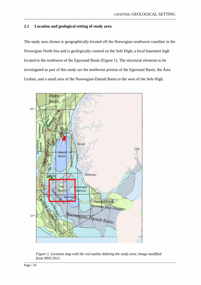
2.1 Location and geological setting of study area
The study area chosen is geographically located off the Norwegian southwest coastline in the
Norwegian North Sea and is geologically centred on the Sele High; a local basement high
located to the northwest of the Egersund Basin (Figure 1). The structural elements to be
investigated as part of this study are the northwest portion of the Egersund Basin, the Åsta
Graben, and a small area of the Norwegian-Danish Basin to the west of the Sele High.
Figure 1. Location map with the red outline defining the study area. Image modified
from NPD 2011.
CHAPTER: GEOLOGICAL SETTING
Page | 11
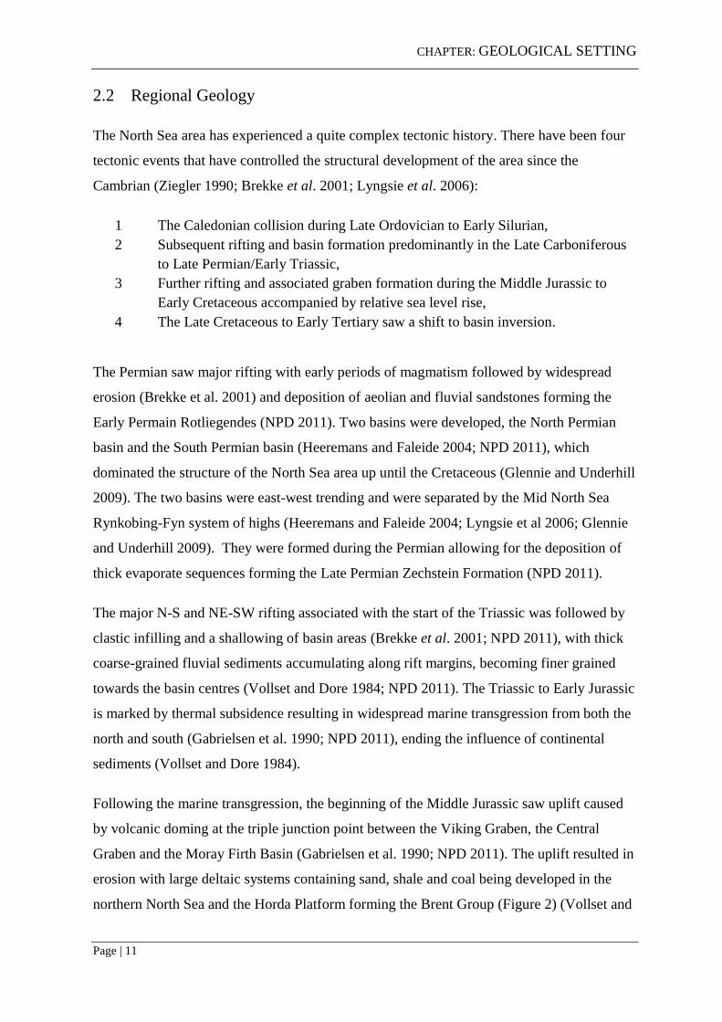
2.2 Regional Geology
The North Sea area has experienced a quite complex tectonic history. There have been four
tectonic events that have controlled the structural development of the area since the
Cambrian (Ziegler 1990; Brekke et al. 2001; Lyngsie et al. 2006):
1 The Caledonian collision during Late Ordovician to Early Silurian,
2 Subsequent rifting and basin formation predominantly in the Late Carboniferous
to Late Permian/Early Triassic,
3 Further rifting and associated graben formation during the Middle Jurassic to
Early Cretaceous accompanied by relative sea level rise,
4 The Late Cretaceous to Early Tertiary saw a shift to basin inversion.
The Permian saw major rifting with early periods of magmatism followed by widespread
erosion (Brekke et al. 2001) and deposition of aeolian and fluvial sandstones forming the
Early Permain Rotliegendes (NPD 2011). Two basins were developed, the North Permian
basin and the South Permian basin (Heeremans and Faleide 2004; NPD 2011), which
dominated the structure of the North Sea area up until the Cretaceous (Glennie and Underhill
2009). The two basins were east-west trending and were separated by the Mid North Sea
Rynkobing-Fyn system of highs (Heeremans and Faleide 2004; Lyngsie et al 2006; Glennie
and Underhill 2009). They were formed during the Permian allowing for the deposition of
thick evaporate sequences forming the Late Permian Zechstein Formation (NPD 2011).
The major N-S and NE-SW rifting associated with the start of the Triassic was followed by
clastic infilling and a shallowing of basin areas (Brekke et al. 2001; NPD 2011), with thick
coarse-grained fluvial sediments accumulating along rift margins, becoming finer grained
towards the basin centres (Vollset and Dore 1984; NPD 2011). The Triassic to Early Jurassic
is marked by thermal subsidence resulting in widespread marine transgression from both the
north and south (Gabrielsen et al. 1990; NPD 2011), ending the influence of continental
sediments (Vollset and Dore 1984).
Following the marine transgression, the beginning of the Middle Jurassic saw uplift caused
by volcanic doming at the triple junction point between the Viking Graben, the Central
Graben and the Moray Firth Basin (Gabrielsen et al. 1990; NPD 2011). The uplift resulted in
erosion with large deltaic systems containing sand, shale and coal being developed in the
northern North Sea and the Horda Platform forming the Brent Group (Figure 2) (Vollset and

CHAPTER: GEOLOGICAL SETTING
Page | 12
Dore 1984; NPD 2011). Similar deltaic systems formed the Vestland Group in the
Norwegian- Danish Basin, the Stord Basin, and the Central Graben and were overlain by
shallow marine to marginal marine sandstones (Vollset and Dore 1984; NPD 2011). Lower
Jurassic marine sediments are absent in much of the area south of the Ling Depression and
Egersund basin presumably due the erosion associated with the uplift (Vollset and Dore
1984).
Figure 2. Examples of mid Jurassic relationship between continental and marine deposits in
central and northern North Sea. Continental sediments in brownish colour, shallow marine
in yellow and offshore marine in blue. The development of the Brent delta and the early
stage of the deposition of the Bryne Formation (left), and the development of the Sognefjord
delta and the Sandnes and Hugin Formations after the Brent delta was transgressed (right).
Image source: CO2 Atlas, NPD 2011.
By the end of the Middle Jurassic, marine conditions had returned as a result of rising sea
levels and the collapse of the uplifted volcanic dome (Vollset and Dore 1984). Shales
accumulated in the basin centres and marginal marine sands were deposited along the basin
margins (Vollset and Dore 1984).
CHAPTER: GEOLOGICAL SETTING
Page | 13
Renewed rifting in the North Sea area took place during the Late Jurassic and lasted into the
Early Cretaceous (Brekke et al. 2001; Vollset and Dore 1984; NPD 2011). Major block
faulting and tilting lead to uplift and erosion with periods of non-deposition (Vollset and
Dore; NPD 2011). Subsequent to this Late Jurassic tectonic activity, rifting ceased and was
followed by thermal subsidence (NPD 2011). Large basins began to subside as sea levels
rose throughout the Cretaceous (Brekke et al. 2001) but by the latest Cretaceous infilling had
resulted in the northern North Sea becoming a wide, low-relief shallow basin (Gabrielsen et
al. 2010). Sediment was sourced from the emerging East Shetland Platform and Scottish
Highlands in the west, and the Norwegian mainland in the east (Faleide et al. 2002;
Gabrielsen et al. 2010).
In the North Sea, deposition of chalk that had started during the Cretaceous continued until
Early Paleocene, which also saw the onset of sea-floor spreading in the North Atlantic and
mountain building in the Alps/Himalayas (Brekke et al. 2001; NPD 2011). During the
Oligocene there appears to have been uplift of basin margins due to inversion (Gabrielsen et
al. 2010; NPD 2011), producing a series of submarine fans with sediments sourced from the
Shetland Platform to the west (NPD 2011). The Rogaland and Hordaland Groups were
formed by these submarine fans interfingering with marine shales, leading to a deltaic
system developing towards the Norwegian North Sea and forming the Skade and Utsira
Formations (NPD 2011). In the Neogene, sediment input was the result of major uplift and
glacial erosion (Brekke et al. 2001; NPD 2011), resulting in thick sequences being deposited
in the North Sea. This had the effect of burying Jurassic source rocks to depths capable of
generating hydrocarbons (NPD 2011).
2.3 Ling Depression
The Ling Depression (Figure 3) acts as a divider between the Utsira High in the north and
the Sele High in the south (Heeremans and Faleide 2004). Together with the Åsta Graben, it
forms the northern limit of the Zechstein basin (Heeremans and Faleide 2004).
Figure 3 shows a cross-section through the southern part of the Ling Depression, the Sele
High and the Åsta Graben.

CHAPTER: GEOLOGICAL SETTING
Page | 14
2.4 Sele High
The Sele High is a shallow basement feature developed locally to the north west of the
Egersund Basin, the south-southeast of the Ling Depression, the Åsta Graben to the
northeast, and the Fiskebank Sub-Basin to the southwest (Figure 3).
Figure 3. Diagrammatic cross section showing the Ling Depression, Sele High and the Åsta
Graben. Image source: Heeremans and Faleide 2004.
2.5 Egersund Basin
The Egersund Basin is a small extensional basin situated approximately 100 km west of the
southernmost part of Norway (Hermanrud et al. 1990). It is a symmetrical basin with its
main depositional axis running NNW-SSE (Figure 1)
The Egersund Basin has been heavily affected by halokinesis and diapirism with Late
Permian Zechstein salt having been intersected in ten wells and halokinetic movements
observed in numerous seismic lines throughout the basin (Figure 4) (Sorensen and Tangen
1995).
The Egersund Basin differs from the graben areas to the west, insofar as it is not part of the
main extensional zone of the Central and Viking Grabens (Hermanrud et al. 1990; Sorensen
and Tangen 1995). Rather it is more structurally related to the evolution of the Norwegian-
Danish Basin (Sorensen and Tangen 1995). The Late Jurassic were relatively quiet tectonic
times throughout the Egersund Basin in contrast to the Central and Viking Grabens
CHAPTER: GEOLOGICAL SETTING
Page | 15
(Sorensen and Tangen 1995). The Egersund Basin was less affected by the heating related to
the late Jurassic stretching, experiencing subsidence and local inversion but to a lesser extent
(Hermanrud et al. 1990; Sorensen and Tangen 1995).
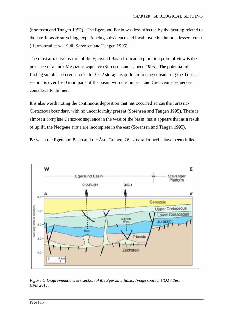
The most attractive feature of the Egersund Basin from an exploration point of view is the
presence of a thick Mesozoic sequence (Sorensen and Tangen 1995). The potential of
finding suitable reservoir rocks for CO2 storage is quite promising considering the Triassic
section is over 1500 m in parts of the basin, with the Jurassic and Cretaceous sequences
considerably thinner.
It is also worth noting the continuous deposition that has occurred across the Jurassic-
Cretaceous boundary, with no unconformity present (Sorensen and Tangen 1995). There is
almost a complete Cenozoic sequence in the west of the basin, but it appears that as a result
of uplift, the Neogene strata are incomplete in the east (Sorensen and Tangen 1995).
Between the Egersund Basin and the Åsta Graben, 26 exploration wells have been drilled
Figure 4. Diagrammatic cross section of the Egersund Basin. Image source: CO2 Atlas,
NPD 2011.

CHAPTER: GEOLOGICAL SETTING
Page | 16
2.6 Åsta Graben
The Åsta Graben is a west-tilted half graben with its main depositional axis trends N-S
(Figure 3). It is less affected by halokinetic movements than the neighbouring Egersund
Basin, which it is separated from by a ridge running approximately east-west (Sorensen and
Tangen 1995).
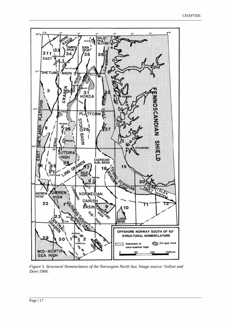
2.7 Fiskebank Sub-Basin and the Norwegian-Danish Basin
The Fiskebank Sub-Basin is an ENE trending sub-basin that is actually the western extension
of the regionally significant Norwegian-Danish Basin (Figure 5) (Pegrum 1984). The
Fiskebank Sub-Basin was transgressed from the east during the Early Jurassic, when
deposition of the Fjerritslev Formation shales was under way (Cope et al 1992).
The Norwegian-Danish Basin (Figure 5) is a WNW-ESE trending basin mainly of Permian
to Early Jurassic age situated in the North Sea between Norway and Denmark (Hospers &
Holthe 1984; Hospers et al. 1988), and is filled with sediments that are in places 8 km thick
(Hospers et al. 1988). The Upper Permian Zechstein salt occurs throughout the basin giving
rise to the widespread and in places, severe salt tectonics (Hospers & Holthe 1984; Hospers
et al. 1988).
The Norwegian-Danish Basin is defined by the Ringkobing-Fyn High to the south, the
Central Graben and adjacent highs to the southwest and west, the Horda Platform to the
northwest and the Fennoscandian Shield to the north and northeast (Hospers et al. 1988). It
comprises a number of distinct tectonic sub-units which are the focus of this thesis (Figure
5).
CHAPTER:
Page | 17
Figure 5. Structural Nomenclature of the Norwegian North Sea. Image source: Vollset and
Dore 1984.

CHAPTER: STRATIGRAPHY
Page | 18
3. STRATIGRAPHY
CHAPTER: STRATIGRAPHY
Page | 19
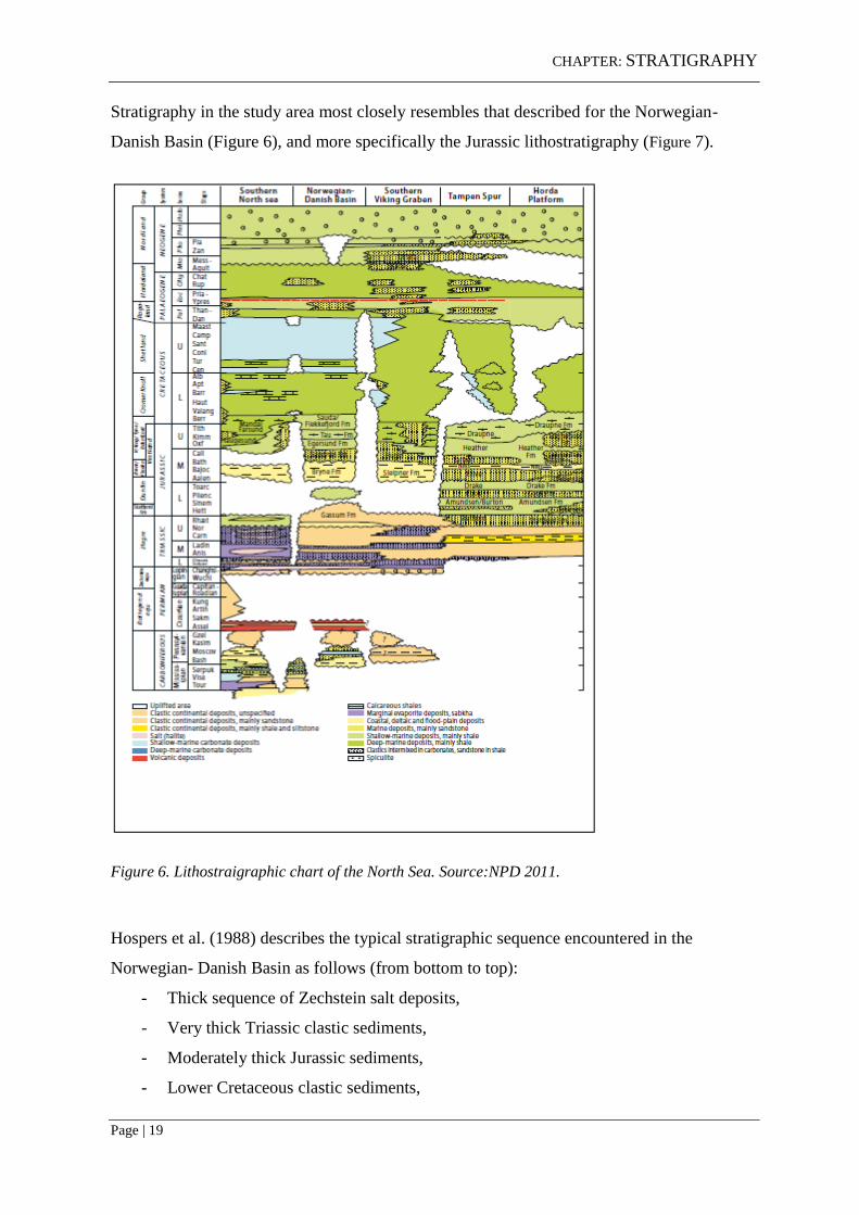
Stratigraphy in the study area most closely resembles that described for the Norwegian-
Danish Basin (Figure 6), and more specifically the Jurassic lithostratigraphy (Figure 7).
Figure 6. Lithostraigraphic chart of the North Sea. Source:NPD 2011.
Hospers et al. (1988) describes the typical stratigraphic sequence encountered in the
Norwegian- Danish Basin as follows (from bottom to top):
- Thick sequence of Zechstein salt deposits,
- Very thick Triassic clastic sediments,
- Moderately thick Jurassic sediments,
- Lower Cretaceous clastic sediments,

CHAPTER: STRATIGRAPHY
Page | 20
- Upper Cretaceous (and locally also Danian) limestone,
- Overlain by very thick Tertiary clastic sediments, and
- Relatively thin Quaternary deposits.
Figure 7. Jurassic lithostratigraphic nomenclature for the central North Sea - Norwegian
Danish Basin. Source: Vollset & Dore 1984.
3.1 Reservoir rocks
The most prospective reservoir rocks in the study area are the Lower Jurassic Sandnes
Formation and to a lesser extent the Bryne Formation (Figure 8). The majority of petroleum
exploration has focused on the Sandnes Formation and several oil discoveries have been
made at this stratigraphic level. Other possibilities are the Late Triassic-Early Jurassic
Gassum Formation, which is developed locally throughout the Norwegian-Danish Basin, and
the Late Triassic Skagerrak Formation, which is well developed throughout the study area.
There have been a number of small hydrocarbon discoveries made in the Egersund Basin and
Asta Graben, with only the 9/2-1 discovery seriously evaluated for development (Sorensen
and Tangen 1995). The high proportion of dry wells has reduced the exploration interest in
these areas over the years, which means there has been relatively less focus on understanding
potential play concepts than some of the more productive areas in the North Sea.

CHAPTER: STRATIGRAPHY
Page | 21
Figure 8. Diagram illustrating the depositional systems of potential CO2 reservoirs of the
North Sea. (Image source: NPD 2011)
3.1.1 Sandnes Formation
The Sandnes Formation is part of the Vestland Group and was deposited in a coastal to
shallow marine environment (Figure 8). It is generally developed as a well-sorted and widely
distributed sand (Figure 9) (NPD 2011), and in the type well (9/4-3) it consists of a massive
white, very fine to coarse-grained glauconitic sandstone (NPD 2012). It is firm to friable,
and in parts, poorly sorted and slightly silty. Towards the eastern margin of the Egersund
Basin in the reference well 18/11-1, the formation comprises interbedded sandstones and
shales (NPD 2012).
The Sandnes Formation usually overlies the non-marine Bryne Formation or older Jurassic
or Triassic rocks unconformably (NPD 2012).

CHAPTER: STRATIGRAPHY
Page | 22
The Sandnes Formation is distributed throughout the Fiskebank Sub-Basin and in the
Egersund Basin and is broadly equivalent to the Hugin Formation in the southern Viking
Graben (NPD 2012).
Figure 9. Plan showing the thickness and distribution of the Sandnes Formation in
the study area.
3.1.2 Bryne Formation
The Bryne Formation conformably underlies the Sandnes Formation and is dominated by
fluvial to non-marine deposits. There is a hiatus in age between the two formations but the
two have a somewhat similar seismic signature making them difficult to distinguish. The
Bryne Formation has a higher clay content compared to the Sandnes Formation reducing its
reservoir properties (Sorensen and Tangen 1995).
The Bryne Formation consists of interbedded sandstones, siltstones, shales and coals. The
sandstones are white to grey, very fine to coarse grained, poorly sorted, friable to hard and
occasionally kaolinitic (NPD 2012).

CHAPTER: STRATIGRAPHY
Page | 23
The Bryne Formation is developed throughout the Norwegian-Danish Basin (Figure 10) and
in the Central Graben and is approximately equivalent in age and lithofacies to the Sleipner
Formation of the Southern Viking Graben (NPD 2012).
Figure 10 Bryne thickness contours over the study area. Image created by author using
NPD data.

CHAPTER: STRATIGRAPHY
Page | 24
3.1.3 Gassum Formation
In the Norwegian sector, the Gassum Formation is predominantly a white to light grey,
mainly fine to medium grained sandstone, but frequently contains coarse sand and gravel. It
is often calcite cemented and in some instances contains glauconite (NPD 2012).
The Gassum Formation occurs throughout the Norwegian-Danish Basin, on the Southern
Vestland Arch and along the northeastern margin of the Central Graben but it is often
completely or partially eroded as a result of mid-Jurassic earth movements (NPD 2012).
The Gassum Formation is possibly equivalent to the Stratfjord Formation but correlation is
uncertain (Vollset and Dore 1984). To overcome this, Vollset and Dore (1984) recommend
using the Gassum Formation south of the Ling Depression. Given that the study area is south
of the Ling Depression, the name Gassum Formation has been adopted herein.
The Gassum Formation hasn’t been studied from a sedimentological point of view in the
Norwegian sector, but it is thought to be deposited as fluvial to marginal marine deposits laid
down during a transgressive phase at the Triassic/Jurassic transition (NPD 2012).
3.1.4 Skagerrak Formation
The Skagerrak Formation consists of poor to moderate sorted sandstones and conglomerates
with interbedded siltstones and shales (Deegan and Scull 1977; Nielsen et al. 2011).
It was deposited as alluvial fan and braided river sediments (Nielsen et al. 2011; NPD 2011),
with the majority of the formation being deposited in a prograding system of alluvial fans
along the eastern and southern flanks of a structurally controlled basin (Deegan and Scull
1977).
The Skagerrak Formation is present throughout the Central North Sea and the western
Skagerrak but is most likely absent over structural highs due to erosion and in some cases
halokinesis (NPD 2011).

CHAPTER:
Page | 25

CHAPTER: THEORETICAL BACKGROUND
Page | 26
4. THEORETICAL BACKGROUND

CHAPTER: THEORETICAL BACKGROUND
Page | 27
4.1 Geological storage of carbon dioxide (CO2)
4.1.1 The need for CO2 storage
Forward modelling by the International Energy Agency (IEA) shows that global energy
demand is set to increase by 40 per cent between now and 2030 with 80 per cent of this
energy demand being met by fossil fuels (Figure 11) (CO2 CRC 2011). This increase in
demand for fossil fuels is likely to be met by coal, particularly for electricity generation in
China and India (CO2 CRC 2011). This is despite a rapid increase in the use of renewable
energy like wind, solar and geothermal. It will be a huge challenge to change the way we
generate electricity and fuel, particularly for energy hungry developing countries like China
and India who are able to grow at such a rate due partly to the cheap source of energy that
coal and other fossil fuels provide.
Figure 11. World energy demand expands by 40%between now and 2030 –an average rate of
increase of 1.5% per year – with coal accounting for more than a third of the overall rise (Data for
graph obtained from World Energy Outlook - OECD/IEA 2009)
The widespread practice of carbon capture and storage (CCS) would allow for a more
gradual transition from the world we live in today where we are heavily dependent on fossil
fuels for our energy needs, to one where we can rely solely on renewable sources of energy.
It would be next to impossible for industries and households alike to switch overnight from
fossil fuels to renewable energy. Renewable energy technologies are not advanced enough to
meet the world’s energy needs, nor are the world’s economies ready for such a dramatic

CHAPTER: THEORETICAL BACKGROUND
Page | 28
shift. CCS has the potential to be an effective transition technology whereby industry
emissions on climate change are minimised while simultaneously minimising the impact on
global economies and energy and electricity generation. (IEA 2008; IPCC 2005)
The capture and storage of carbon dioxide is an important mitigation tool for the overall
reduction of anthropogenic CO2 emissions. However, it cannot be seen as a cure all for the
problem, but rather one weapon in the arsenal against climate change. Techniques such as
enhanced oil recovery (EOR) using CO2, for example, could form an integral part of the
solving two big problems; where to store all this excess CO2? And how do we extract the
worlds diminishing oil supplies in the most efficient and responsible way?
4.1.2 What is Carbon Capture and Storage (CCS)?
The most widely recognised form of carbon capture and storage involves the capture of CO2
from major stationary point sources that would otherwise be emitted into the atmosphere,
such as coal fired power plants and heavy industry, compressing the CO2 into a supercritical
liquid and storing it deep underground in porous rock formations (CSIRO 2011; IEA 2008).
This is known as geological storage, geological sequestration or geosequestration (IEA
2008). Other forms of CCS involve biological storage and ocean storage.
The geological storage of CO2 is a process that has been occurring naturally in the Earth’s
subsurface for hundreds of millions of years. Indeed, this is where most of the world’s
carbon is held; in coals, oil, gas, organic-rich shales and carbonate rocks (IPCC 2005).
Therefore, it is that the same geological forces that have naturally held CO2 will be the same
principles under which injected CO2 will be held (IEA 2008). After the CO2 is injected it will
be trapped in tiny pores within the rock formations far below the surface, separated from
fresh groundwater by thick, impermeable layers of rock (Figure 12) (IEA 2008).
What many government organisations, research institutes and private investors are now
doing is building on the knowledge of this natural process in the hope of using CO2 storage
as a mitigation option for reducing their CO2 emissions. A good example of this is coal-fired
power generators that are hugely important to many countries in terms of power generation
but are also huge stationary CO2 emitters; a prime candidate for carbon capture and storage.
Figure 13 shows how this might work.

CHAPTER: THEORETICAL BACKGROUND
Page | 29
Figure 12. Illustration of the separation between the deep saline aquifers to be used for CO2 storage
and the fresh water aquifers much closer to the surface. Image source: CO2CRC 2011.
Figure 13. Illustration of the main processes at work in a CCS operation. Image source: CO2CRC

CHAPTER: THEORETICAL BACKGROUND
Page | 30
4.1.3 How is CO2 stored?
In order to store CO2 in geological formations, it must first be compressed to form a super
critical liquid. The degree to which the CO2 is compressed is dependent on temperature and
pressure and therefore the amount of compression increases with depth. This means the
amount of space taken up by the supercritical CO2 decreases as depth increases. (IPCC
2005; IEA 2008)
After the CO2 has been compressed, it must pumped into a suitable rock formation or
reservoir. For example, this could be deep unmined coal seams, depleted oil fields or deep
saline aquifers (IPCC 2005; IEA 2008).
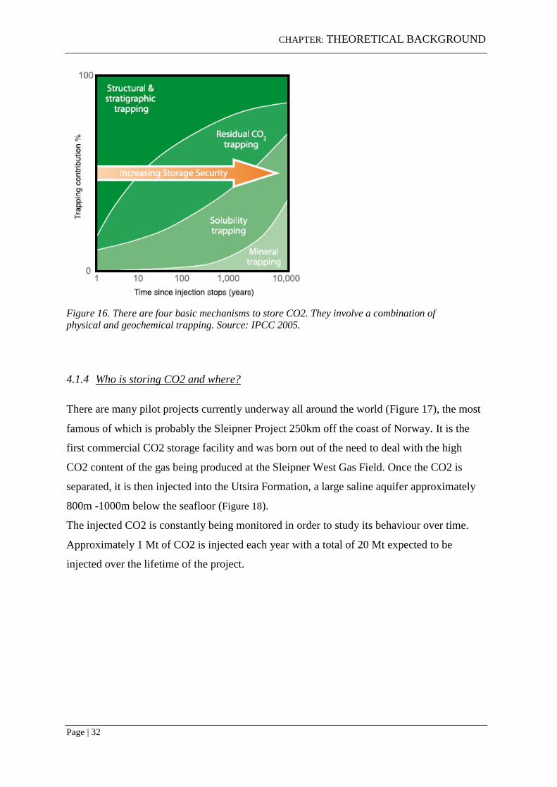
The storage of CO2, once in a supercritical state, involves trapping the CO2 by way of
either physical trapping or geochemical trapping. According to Chadwick et al. (2008) there
are four basic mechanisms with which this can be achieved (Figure 16):
Structural and stratigraphical trapping (Figure 15) occurs where the migration of free
(gas, liquid, fluid) CO2 in response to its buoyancy and/or pressure gradients within
the reservoir is prevented by low permeability barriers (caprocks) such as layers of
mudstone or halite.
Residual saturation trapping occurs when capillary forces and adsorption onto the
surfaces of mineral grains within the rock matrix immobilise a proportion of the
injected CO2 along its migration path (Figure 14).
Figure 14 illustrates the residual trapping of CO2. Source: CO2CRC 2012

CHAPTER: THEORETICAL BACKGROUND
Page | 31
Figure 15 Examples of structural and stratigraphic traps for CO2: (a) anticline
structural traps; (b) fault structural trap; (c) pinchout and lateral facies change
stratigraphic traps; and (d) unconformity stratigraphic trap. Source: Gibson-Poole
Dissolution trapping occurs where injected CO2 dissolves and becomes trapped
within the reservoir brine.
Geochemical trapping occurs when in which dissolved CO2 reacts with the native
pore fluid and/or the minerals making up the rock matrix of the reservoir. CO2 is
incorporated into the reaction products as solid carbonate minerals and aqueous
complexes dissolved in the formation water.
CHAPTER: THEORETICAL BACKGROUND
Page | 32
Figure 16. There are four basic mechanisms to store CO2. They involve a combination of
physical and geochemical trapping. Source: IPCC 2005.
4.1.4 Who is storing CO2 and where?
There are many pilot projects currently underway all around the world (Figure 17), the most
famous of which is probably the Sleipner Project 250km off the coast of Norway. It is the
first commercial CO2 storage facility and was born out of the need to deal with the high
CO2 content of the gas being produced at the Sleipner West Gas Field. Once the CO2 is
separated, it is then injected into the Utsira Formation, a large saline aquifer approximately
800m -1000m below the seafloor (Figure 18).
The injected CO2 is constantly being monitored in order to study its behaviour over time.
Approximately 1 Mt of CO2 is injected each year with a total of 20 Mt expected to be
injected over the lifetime of the project.

CHAPTER: THEORETICAL BACKGROUND
Page | 33
Figure 17.Geologic storage and related projects are in operation or proposed around the
world. Most are research, development or demonstration projects. Several are part of
industrial facilities in commercial operation. Image Source: CO2CRC 2012.
Figure 18 shows a simplified diagram of the Sleipner Project. Source: IPCC 2005
CHAPTER: THEORETICAL BACKGROUND
Page | 34
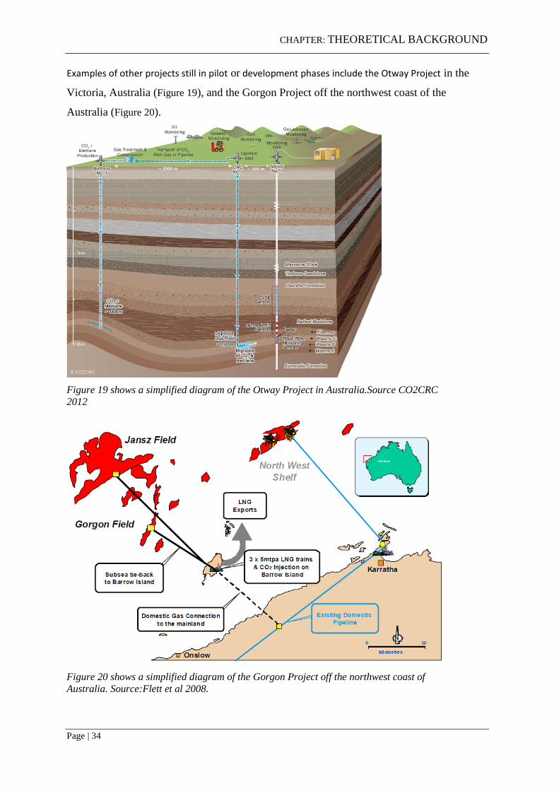
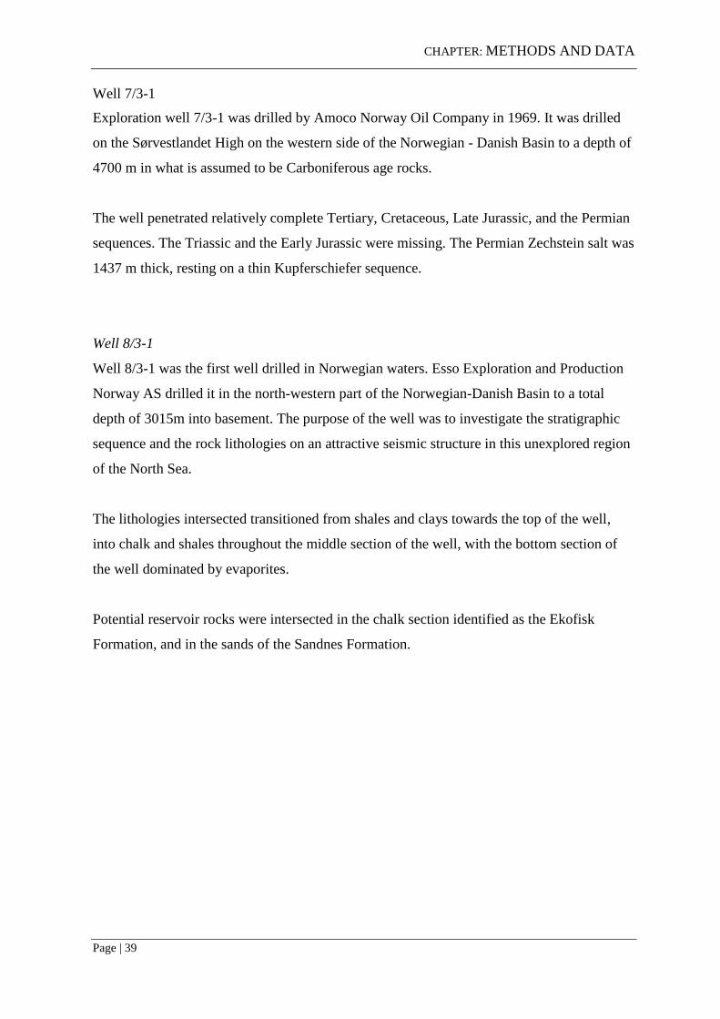
Examples of other projects still in pilot or development phases include the Otway Project in the
Victoria, Australia (Figure 19), and the Gorgon Project off the northwest coast of the
Australia (Figure 20).
Figure 19 shows a simplified diagram of the Otway Project in Australia.Source CO2CRC
2012
Figure 20 shows a simplified diagram of the Gorgon Project off the northwest coast of
Australia. Source:Flett et al 2008.

CHAPTER: THEORETICAL BACKGROUND
Page | 35
4.2 Classification / ranking schemes used in the CO2 Atlas
The Norwegian Petroleum Directorate (NPD) has developed a checklist as a way of
classifying reservoirs and their seals (Figure 20). It was used as a screening tool as part of
this study to help determine the most appropriate parameter cut offs.
.
Figure 21 Checklists for reservoir and sealing properties. Source: NPD 2011

CHAPTER: METHODS AND DATA
Page | 36
5. METHODS AND DATA

CHAPTER: METHODS AND DATA
Page | 37
5.1 Dataset
This study focuses on eight wells that were selected based on their geographic location;
wells 18/10-1 located in the NW Egersund Basin, wells 17/11/1 and 17/11-2 on the margins
of the Sele High, 17/4-1 in the Ling Depression, 17/9-1 in the Åsta Graben, and wells 17/10-
1, 7/3-1 and 8/4-1 in the Fiskebank Sub-basin.
5.1.1 Wells
There are eight wells used as part of the thesis: 7/3-1, 8/3-1, 17/9-1, 17/10-1, 17/11-1, 17/11-
2, 17/4-1, 18/10-1 (Figure 22). The wells were used for stratigraphic control when
interpreting the seismic data away from well control and to calculate properties of the
interpreted sequences. They were particularly useful when calculating properties such as
porosity and permeability to determine reservoir suitability. After initial screening, which
included well log and seismic analysis, two wells were determined to have the most suitable
reservoir properties for CO2 storage. These were well 17/10-1 located in the Åsta Graben
adjacent to the Sele High, and well 18/10-1 in the NW Egersund Basin.

CHAPTER: METHODS AND DATA
Page | 38
Figure 22. Location plan showing location of wells in the study area. Source??
CHAPTER: METHODS AND DATA
Page | 39
Well 7/3-1
Exploration well 7/3-1 was drilled by Amoco Norway Oil Company in 1969. It was drilled
on the Sørvestlandet High on the western side of the Norwegian - Danish Basin to a depth of
4700 m in what is assumed to be Carboniferous age rocks.
The well penetrated relatively complete Tertiary, Cretaceous, Late Jurassic, and the Permian
sequences. The Triassic and the Early Jurassic were missing. The Permian Zechstein salt was
1437 m thick, resting on a thin Kupferschiefer sequence.
Well 8/3-1
Well 8/3-1 was the first well drilled in Norwegian waters. Esso Exploration and Production
Norway AS drilled it in the north-western part of the Norwegian-Danish Basin to a total
depth of 3015m into basement. The purpose of the well was to investigate the stratigraphic
sequence and the rock lithologies on an attractive seismic structure in this unexplored region
of the North Sea.
The lithologies intersected transitioned from shales and clays towards the top of the well,
into chalk and shales throughout the middle section of the well, with the bottom section of
the well dominated by evaporites.
Potential reservoir rocks were intersected in the chalk section identified as the Ekofisk
Formation, and in the sands of the Sandnes Formation.

CHAPTER: METHODS AND DATA
Page | 40
Well 17/4-1
Well 17/4-1 was drilled by Elf Petroleum Norge AS in 1968 to a depth of 3997m. It was
drilled on a NNE-SSW trending monocline in the Ling Depression with the objective to test
the hydrocarbon potential of the Mesozoic sands.

CHAPTER: METHODS AND DATA
Page | 41
The well encountered Jurassic and Triassic sandstones with medium to good porosities but
mostly poor permeabilities due to calcite cement. The stratigraphic units intersected are
illustrated in the well panel below (Figure 23).
Figure 23 Stratigraphic units and log for well 17/4-1.
Well 17/9-1
Well 17/9-1 was drilled by Esso Exploration and Production Norway A/S in 1973 to a depth
of 2816m before being re-entered as 17/9-1R and drilled to a total depth of 3161m. It was
drilled in the Åsta Graben approximately 30km north of the 17/12-1R Discovery well with
the primary objective to investigate the sands at the base of the Jurassic sequence.
Well 17/9-1 was found to have no rocks with any reservoir potential. The stratigraphic units
intersected are illustrated in the well panel below (Figure 24).

CHAPTER: METHODS AND DATA
Page | 42
Figure 24 Stratigraphic units and log for well 17/9-1.

CHAPTER: METHODS AND DATA
Page | 43
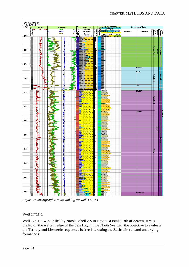
Well 17/10-1
Well 17/10-1 was drilled by Norske Shell AS in 1968 to a total depth of 3591m. It was
drilled in the Norwegian-Danish Basin near the western margin of the Sele High. The
objective was to test the Mesozoic section of a gentle anticline in an area with prominent salt
walls.
The massive Jurassic and Triassic sandstones of the Gassum and Skagerrak Formations were
intersected with promising porosities of between 20% to 25%. The stratigraphic units
intersected are illustrated in the well panel below (Figure 25).
CHAPTER: METHODS AND DATA
Page | 44
Figure 25 Stratigraphic units and log for well 17/10-1.
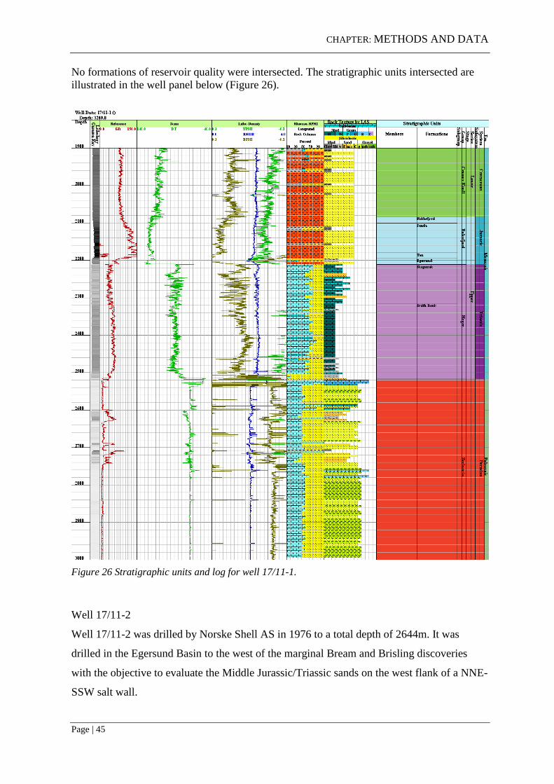
Well 17/11-1
Well 17/11-1 was drilled by Norske Shell AS in 1968 to a total depth of 3269m. It was
drilled on the western edge of the Sele High in the North Sea with the objective to evaluate
the Tertiary and Mesozoic sequences before interesting the Zechstein salt and underlying
formations.
CHAPTER: METHODS AND DATA
Page | 45
No formations of reservoir quality were intersected. The stratigraphic units intersected are
illustrated in the well panel below (Figure 26).
Figure 26 Stratigraphic units and log for well 17/11-1.
Well 17/11-2
Well 17/11-2 was drilled by Norske Shell AS in 1976 to a total depth of 2644m. It was
drilled in the Egersund Basin to the west of the marginal Bream and Brisling discoveries
with the objective to evaluate the Middle Jurassic/Triassic sands on the west flank of a NNE-
SSW salt wall.

CHAPTER: METHODS AND DATA
Page | 46
The top section of the target Skagerrak Formation showed promising porosities. The
stratigraphic units intersected are illustrated in the well panel below (Figure 27).
Figure 27 Stratigraphic units and log for well 17/11-2.
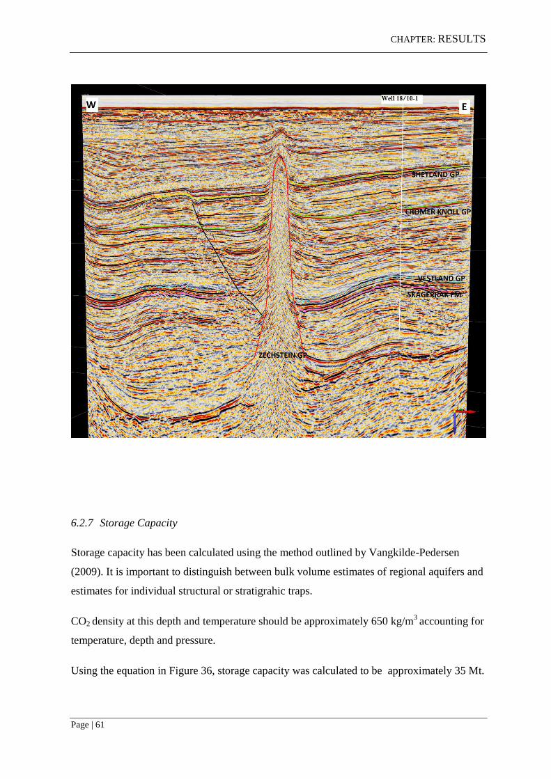
Well 18/10-1
Well 18/10-1 was drilled by Elf Petroleum Norge AS in 1979 to a total depth of 2800m. It
was drilled in the Egersund Basin in the North Sea with the objective to evaluate a seismic
feature on the same trend as the marginal Bream discovery. The target was the Middle
Jurassic sandstones.
The target sands of the Sandnes and Bryne Formations were intersected at 2405m with the
reservoir zone separated by a thin shale barrier. The stratigraphic units intersected are
illustrated in the well panel below (Figure 28).

CHAPTER: METHODS AND DATA
Page | 47
Figure 28 Stratigraphic units and log for well 18/10-1.

CHAPTER: METHODS AND DATA
Page | 48
5.1.2 Well log quality checks
The quality of the well log data can be affected by several environmental factors throughout
the drilling and logging process. The density and porosity logs in particular are important to
the methodology of this study so quality checks were performed on the logs to identify any
irregularities or suspicious readings.
This was done by evaluating the caliper log to check for large variations of the borehole
diameter due to caving, and the density correction log (DRHO), which records absolute
deviations of the log signal. If this deviation exceeds 0.15 or -0.15 g/cm3, the log signal can
no longer be trusted and should be ignored (Ramaekers 2006 in Benedictus 2007).
Caving of the borehole can result in misleading values for density (too low), and porosity
(too high).
5.1.3 Well Log Analysis
Geophysical well logs were analysed and used to calculate various petrophysical parameters
and properties such as porosity (effective and total), permeability, volume of shale, and net-
to-gross ratio. All calculations were done in Microsoft Excel to make it possible to calculate
the various properties for every log interval within the potential reservoir. This enabled the
calculation of hundreds of interval throughout the reservoir and then an average was taken to
give a representative result.
Matrix and fluid densities used as part of these calculations were taken from widely accepted
estimates of 2.65 g/cm3 (quartz/sandstone) and 1.03 cm/3 (formation water) respectively
(see Table 1).
Table 1. Typical values for matrix and fluid densities.
Typical values for matrix and fluid densities (g/cm3)
Sandstone 2.65
Limestone 2.71
Dolomite 2.87
Anhydrite 2.98
Halite 2.03

CHAPTER: METHODS AND DATA
Page | 49
Porosity
Porosity will be estimated using the density log;
ΦD = ρmatrix - ρb / ρmatrix - ρf
Where:
ΦD = Porosity derived from density log
ρmatrix = Matrix density (obtained from Table 1)
ρb = Bulk density from log
ρf = Fluid density (obtained from Table 1)
Permeability
Permeability will be estimated using the concept of Flow Zone Indicator (FZI) as described
by Chandra (2008). Flow Zone Indicator will be obtained from the combined use of the
available well log data. FZI will be calculated for the selected reservoir intervals using the
technique given by Xue and Dutta Gupta (1997). This technique is based on the
transformation of gamma ray (GR), neutron porosity (NPHI), density (RHOB) and resistivity
(LLD) logs as given below:
GR_Tr = 4.7860E-03 GR2 – 1.7320E-01 GR + 1.0614E+00 ------------ -------(3)
NPHI_Tr = -8.1102E+00 NPHI 2 + 9.6676E-01 NPHI + 1.7170E-01 --------- (4)
RHOB_Tr = 7.1926E+00 RHOZ 2 – 3.6727E+01 RHOB + 4. 5873E+01 -----(5)
LLD_Tr = -1.6859E-04 HLLD 2 – 3.8016E-02 LLD + 4. 3712E-01 -------- ---(6)
SUMTr = GR_Tr + NPHI_Tr +RHOB_Tr + LLD_Tr --------------------- -----(7)
FZI = 4.4306E-01 SUMTr2 + 6. 08575E-01 SUMTr + 3.8229E-01 ------------ (8)
Gypsum 2.35
Clay 2.7-2.8
Freshwater 1
Seawater 1.03-1.06
Oil 0.6-0.7
Gas 0.15

CHAPTER: METHODS AND DATA
Page | 50
SUMTr is the sum of all transforms given by equations 3-6. Equation 8 gives the relation
between the logs and FZI.
Volume of shale calculations
Volume of shale can be determined by using any of the described in Figure 29, after which the
lowest estimate should be applied to shale corrections for porosity (Doveton 2001). The
theory is that all the shale equations will overestimate the shale content because there will
generally be other components in the rock other than shale that will lead to increased log
readings of shaliness (Doveton 2001).
Figure 29. Volume of Shale equations.
Net/Gross Ratio
Net-to-gross ratio aims to describe the portion of the reservoir rock which contributes to
production, or in this case storage. It is a notoriously subjective parameter and so is defined
for this study as using the following criteria:

CHAPTER: METHODS AND DATA
Page | 51
Porosity > 15%
Permeability > 10 mD
Vshale < 0.25
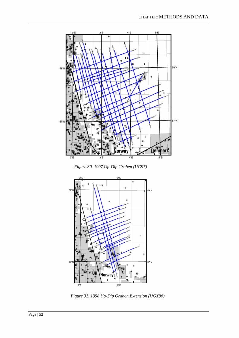
5.2 Seismic surveys
The 2D seismic dataset has been obtained from three separate surveys and covers the parts of
the Asta Graben, Ling Depression, Egersund Basin, Norwegian-Danish Basin and the entire
Sele High. The seismic surveys were:
- The UG97 lines were acquired and processed by Fugro in 1997. The survey was
sponsored by Statoil and was known as 1997 Up-Dip Graben.
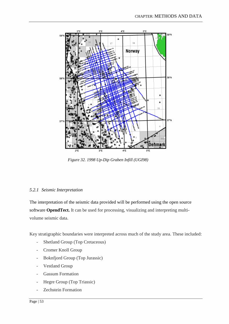
- The UGI98 lines were acquired and processed by Fugro in 1998. The survey was
sponsored by Statoil and was known as 1998 Up-Dip Graben Infill.
- The UGX98 lines were acquired and processed by Fugro and was known as 1998
Up-Dip Graben Extension.
- The UG97 2D seismic survey was acquired by Geco in 1992.
CHAPTER: METHODS AND DATA
Page | 52
Figure 30. 1997 Up-Dip Graben (UG97)
Figure 31. 1998 Up-Dip Graben Extension (UGX98)
CHAPTER: METHODS AND DATA
Page | 53
Figure 32. 1998 Up-Dip Graben Infill (UGI98)
5.2.1 Seismic Interpretation
The interpretation of the seismic data provided will be performed using the open source
software OpendTect. It can be used for processing, visualizing and interpreting multi-
volume seismic data.
Key stratigraphic boundaries were interpreted across much of the study area. These included:
- Shetland Group (Top Cretaceous)
- Cromer Knoll Group
- Boknfjord Group (Top Jurassic)
- Vestland Group
- Gassum Formation
- Hegre Group (Top Triassic)
- Zechstein Formation

CHAPTER:
Page | 54
The seismic reflectors were picked after studying the literature and finding a few reference
seismic lines that had previously been interpreted. In this way, it was possible to build on my
interpretation while being able to tie back to the reference lines. An example of a reference
line used was GLD92-204 (Heeremans and Faleide 2004).
5.2.2 Seismic-to-well tie
A seismic-to-well tie was performed on each of the selected wells using the OpendTect
software. This involved using the well logs for each of the wells and tying them to the 2D
seismic lines that intersect those wells.
5.3 Storage Capacity Calculation
As is the case with the CO2 Atlas published by the Norwegian Petroleum Directorate, the
method for calculating effective storage capacity for a potential CO2 reservoir is shown in
Equation 1.
Equation 1. Equation used for calculating effective storage capacity. Image Source:
Vangkilde-Pedersen 2009.

CHAPTER: RESULTS
Page | 55
6. RESULTS
CHAPTER: RESULTS
Page | 56
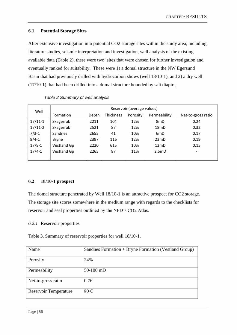
6.1 Potential Storage Sites
After extensive investigation into potential CO2 storage sites within the study area, including
literature studies, seismic interpretation and investigation, well analysis of the existing
available data (Table 2), there were two sites that were chosen for further investigation and
eventually ranked for suitability. These were 1) a domal structure in the NW Egersund
Basin that had previously drilled with hydrocarbon shows (well 18/10-1), and 2) a dry well
(17/10-1) that had been drilled into a domal structure bounded by salt diapirs,
Table 2 Summary of well analysis
Well Reservoir (average values)
Formation Depth Thickness Porosity Permeability Net-to-gross ratio
17/11-1 Skagerrak 2211 104 12% 8mD 0.24
17/11-2 Skagerrak 2521 87 12% 18mD 0.32
7/3-1 Sandnes 2655 41 10% 6mD 0.17
8/4-1 Bryne 2397 116 12% 23mD 0.19
17/9-1 Vestland Gp 2220 615 10% 12mD 0.15
17/4-1 Vestland Gp 2265 87 11% 2.5mD -
6.2 18/10-1 prospect
The domal structure penetrated by Well 18/10-1 is an attractive prospect for CO2 storage.
The storage site scores somewhere in the medium range with regards to the checklists for
reservoir and seal properties outlined by the NPD’s CO2 Atlas.
6.2.1 Reservoir properties
Table 3. Summary of reservoir properties for well 18/10-1.
Name Sandnes Formation + Bryne Formation (Vestland Group)
Porosity 24%
Permeability 50-100 mD
Net-to-gross ratio 0.76
Reservoir Temperature 80ᵒC

CHAPTER: RESULTS
Page | 57
Bottom Hole Temperature 88ᵒC
Thickness 100 m
Area 20 km2
Depth 2405 m
6.2.2 Porosity
Porosity was estimated using the density log (equation 1); and then also calculated by
compensating for Vshale (equation 2). This was done in excel
Equation 1
ΦD = ρmatrix - ρb / ρmatrix - ρf
Where:
ΦD = Porosity derived from density log
ρmatrix = Matrix density
ρb = Bulk density from log
ρf = Fluid density
Equation 2

CHAPTER: RESULTS
Page | 58
The porosity was calculated to be an average of approximately 24%.
Porosity values calculated between 2431-2433m were not included as these were found to be
erroneously high. The caliper log was checked as part of the quality control process and
there was several intervals that were found to be problematic. The caliper log showed a
widening of the well, which can lead to misleading geophysical log readings, in this case
higher than expected neutron porosity readings and lower than expected bulk densities.
6.2.3 Permeability
Permeability was calculated using the Flow Zone Indicator method described in the methods
section. It was calculated to be between 50-100mD.
The above chart shows permeability versus depth to illustrate how permeability changes as
depth increases.

CHAPTER: RESULTS
Page | 59
6.2.4 Net-to-gross ratio
Net-to-gross ratio is a notoriously subjective parameter and so is defined for this study as
using the following criteria:
Porosity > 15%
Permeability > 10 mD
Vshale < 0.25
6.2.5 Seal and caprock
The caprock for this prospect is the regional stratigraphic seal, the Boknfjord Group, which
which consists of several shale formations. This widespread group consists predominantly of
shales, mudstones and claystones, but also includes varying amounts of siltstone, sandstone,
and limestone stringers (NPD 2012). Caprock thickness is approximately 400 metres in this
part of the basin.
The dome structure is broken by minor faulting which defines a kind of slump close to the
top of the structure. Given the thickness of the caprock, this small scale faulting is unlikely
to have any impact on the integrity of the seal.
6.2.6 Trap
The trap type for the 18/10-1 prospect is a structural trap. Underlying salt movement
(halokinesis) has uplifted part of the overlying strata forming a semi-closed domal structure.
When talking about storage capacity for saline aquifers it is important to consider whether
the trap is closed, semi-closed or open, as this will greatly affect the storage efficiency

CHAPTER: RESULTS
Page | 60
factor.
CHAPTER: RESULTS
Page | 61
6.2.7 Storage Capacity
Storage capacity has been calculated using the method outlined by Vangkilde-Pedersen
(2009). It is important to distinguish between bulk volume estimates of regional aquifers and
estimates for individual structural or stratigrahic traps.
CO2 density at this depth and temperature should be approximately 650 kg/m3
accounting for
temperature, depth and pressure.
Using the equation in Figure 36, storage capacity was calculated to be approximately 35 Mt.
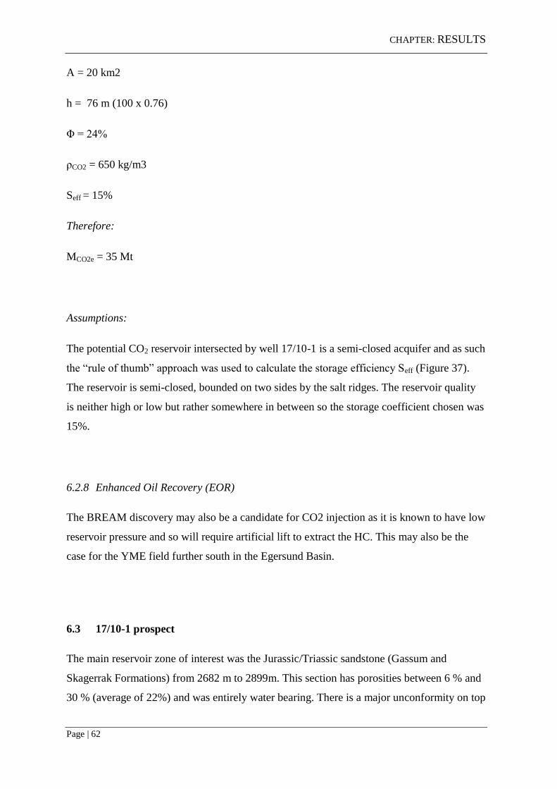
CHAPTER: RESULTS
Page | 62
A = 20 km2
h = 76 m (100 x 0.76)
Φ = 24%
ρCO2 = 650 kg/m3
Seff = 15%
Therefore:
MCO2e = 35 Mt
Assumptions:
The potential CO2 reservoir intersected by well 17/10-1 is a semi-closed acquifer and as such
the “rule of thumb” approach was used to calculate the storage efficiency Seff (Figure 37).
The reservoir is semi-closed, bounded on two sides by the salt ridges. The reservoir quality
is neither high or low but rather somewhere in between so the storage coefficient chosen was
15%.
6.2.8 Enhanced Oil Recovery (EOR)
The BREAM discovery may also be a candidate for CO2 injection as it is known to have low
reservoir pressure and so will require artificial lift to extract the HC. This may also be the
case for the YME field further south in the Egersund Basin.
6.3 17/10-1 prospect
The main reservoir zone of interest was the Jurassic/Triassic sandstone (Gassum and
Skagerrak Formations) from 2682 m to 2899m. This section has porosities between 6 % and
30 % (average of 22%) and was entirely water bearing. There is a major unconformity on top
CHAPTER: RESULTS
Page | 63
of these sands to the overlying Late Jurassic shales. The claystones and mudstones of the
Tau and Egersund Formations overlying the Gassum Formation, had exceptionally high
gamma ray values. These are expected to form part of the seal for this prospect.
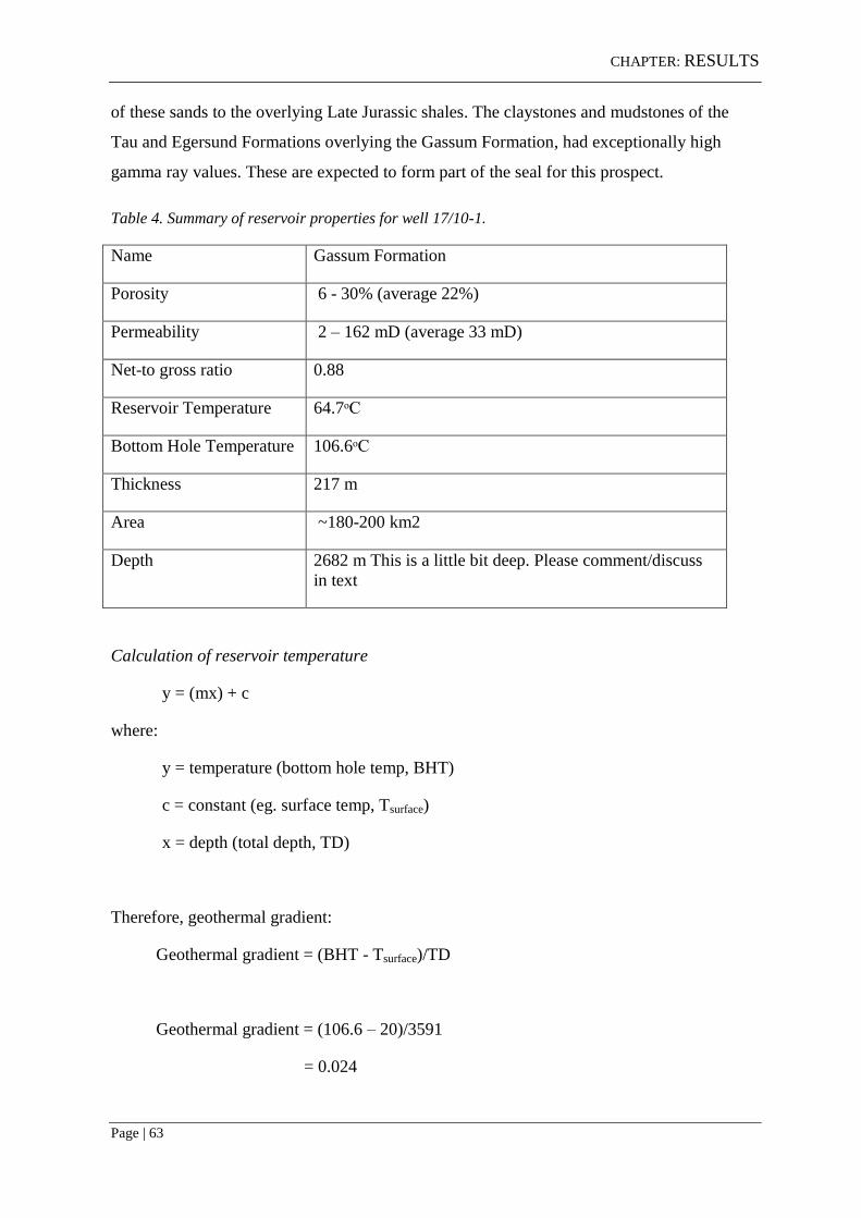
Table 4. Summary of reservoir properties for well 17/10-1.
Name Gassum Formation
Porosity 6 - 30% (average 22%)
Permeability 2 – 162 mD (average 33 mD)
Net-to gross ratio 0.88
Reservoir Temperature 64.7ᵒC
Bottom Hole Temperature 106.6ᵒC
Thickness 217 m
Area ~180-200 km2
Depth 2682 m This is a little bit deep. Please comment/discuss
in text
Calculation of reservoir temperature
y = (mx) + c
where:
y = temperature (bottom hole temp, BHT)
c = constant (eg. surface temp, Tsurface)
x = depth (total depth, TD)
Therefore, geothermal gradient:
Geothermal gradient = (BHT - Tsurface)/TD
Geothermal gradient = (106.6 – 20)/3591
= 0.024

CHAPTER: RESULTS
Page | 64
Therefore:
Reservoir temperature = 0.024 x 2682
= 64.7ᵒC
6.3.1 Porosity
Porosity was estimated using the density log;
ΦD = ρmatrix - ρb / ρmatrix - ρf
Where:
ΦD = Porosity derived from density log
ρmatrix = Matrix density
ρb = Bulk density from log
ρf = Fluid density
Porosity was calculated to be an average 22%.
6.3.2 Permeability
Permeability was calculated using the Flow Zone Indicator method described in the methods
section. It was calculated to be between 2 -162 mD with an average of 33 mD.
6.3.3 Net-to-gross ratio
Net to gross ratio for the Gassum Formation was calculated as 0.88 using the following
conditions/cut-offs:
Porosity greater than 15%
Vshale less then 0.15
Permeability greater than 10 mD
CHAPTER: RESULTS
Page | 65
6.3.4 Seal and caprock
The caprock for this prospect is the regional stratigraphic seal, the Boknfjord Group, which
consists of several shale formations. This widespread group consists predominantly of
shales, but also includes varying amounts of siltstone, sandstone, and limestone stringers
(NPD 2012). Caprock thickness is approximately 150 metres in this part of the basin.
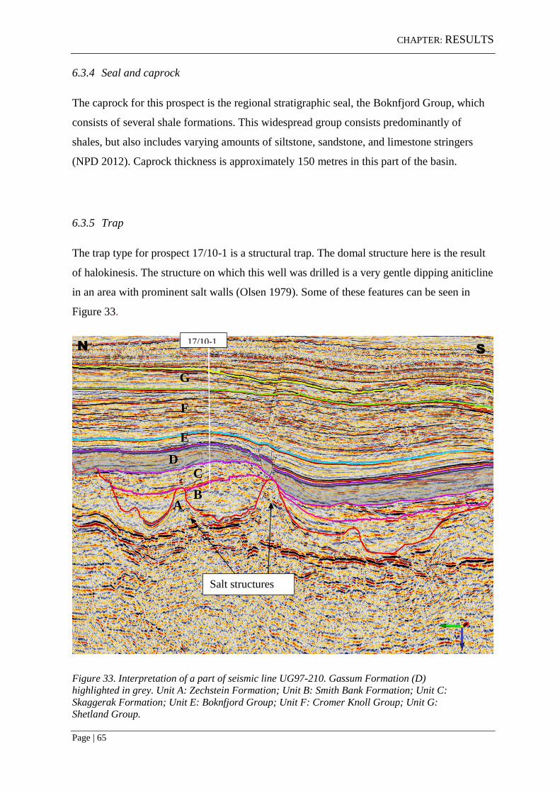
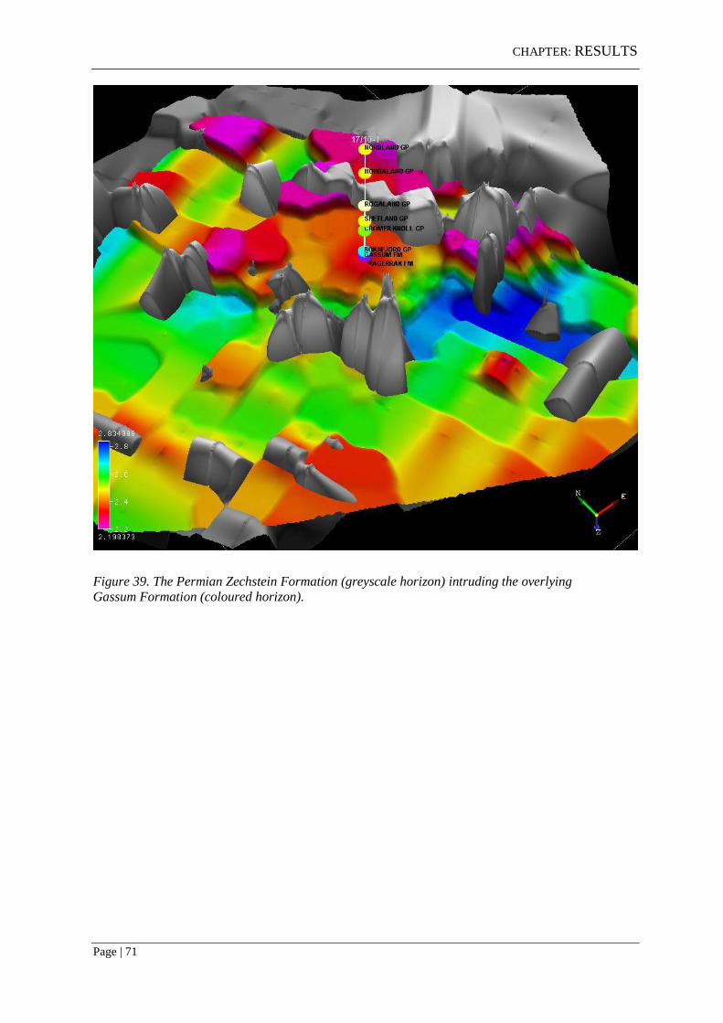
6.3.5 Trap
The trap type for prospect 17/10-1 is a structural trap. The domal structure here is the result
of halokinesis. The structure on which this well was drilled is a very gentle dipping aniticline
in an area with prominent salt walls (Olsen 1979). Some of these features can be seen in
Figure 33.
Figure 33. Interpretation of a part of seismic line UG97-210. Gassum Formation (D)
highlighted in grey. Unit A: Zechstein Formation; Unit B: Smith Bank Formation; Unit C:
Skaggerak Formation; Unit E: Boknfjord Group; Unit F: Cromer Knoll Group; Unit G:
Shetland Group.
B A
C D
E
F
G
17/10-1
Salt structures
N S
CHAPTER: RESULTS
Page | 66
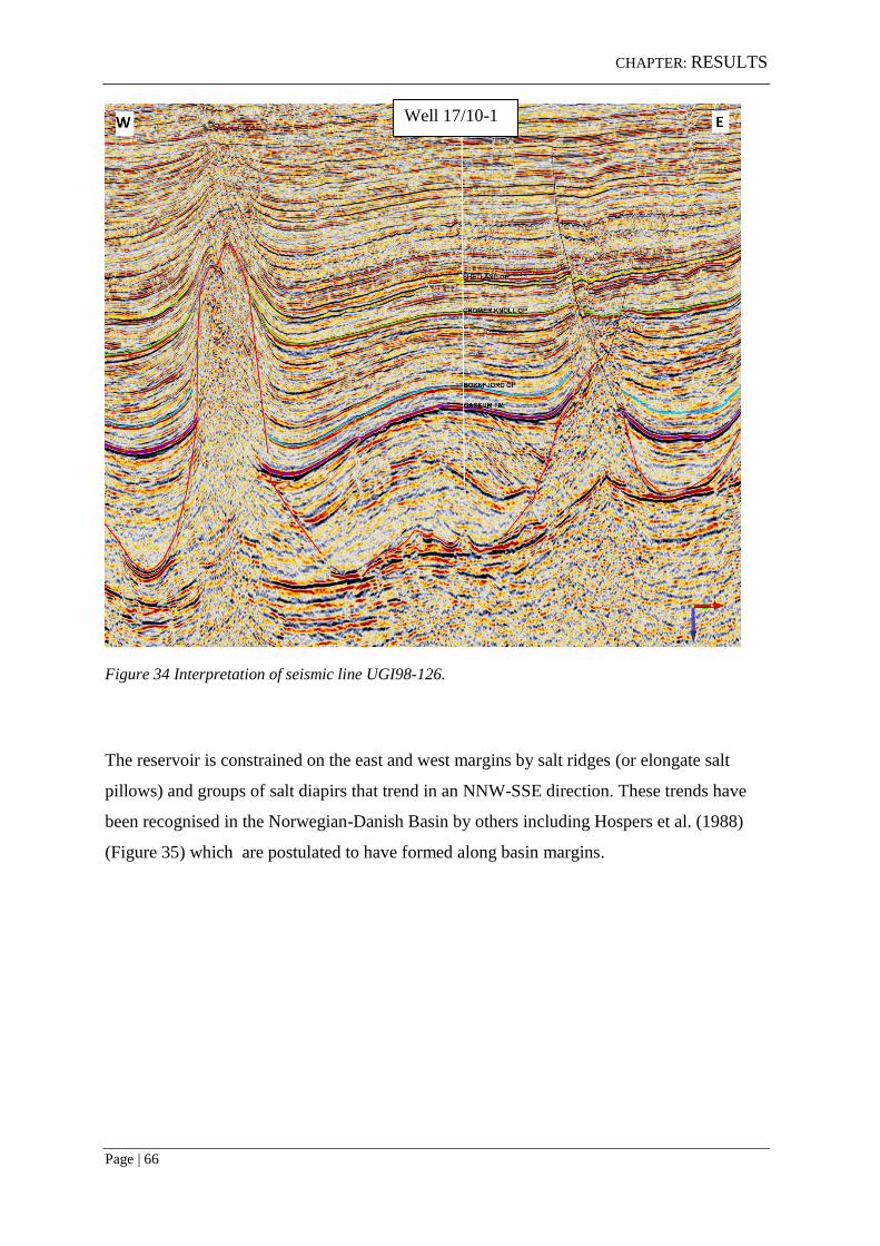
Figure 34 Interpretation of seismic line UGI98-126.
The reservoir is constrained on the east and west margins by salt ridges (or elongate salt
pillows) and groups of salt diapirs that trend in an NNW-SSE direction. These trends have
been recognised in the Norwegian-Danish Basin by others including Hospers et al. (1988)
(Figure 35) which are postulated to have formed along basin margins.
Well 17/10-1

CHAPTER: RESULTS
Page | 67
Figure 35. Map showing position of salt structures and the trend lines through those structures. Image source: Hospers et al. (1988).
CHAPTER: RESULTS
Page | 68
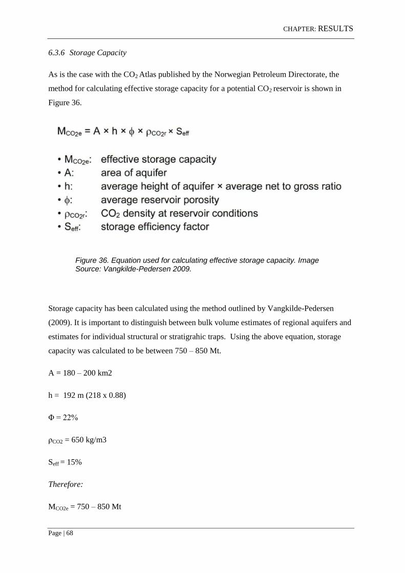
6.3.6 Storage Capacity
As is the case with the CO2 Atlas published by the Norwegian Petroleum Directorate, the
method for calculating effective storage capacity for a potential CO2 reservoir is shown in
Figure 36.
Figure 36. Equation used for calculating effective storage capacity. Image Source: Vangkilde-Pedersen 2009.
Storage capacity has been calculated using the method outlined by Vangkilde-Pedersen
(2009). It is important to distinguish between bulk volume estimates of regional aquifers and
estimates for individual structural or stratigrahic traps. Using the above equation, storage
capacity was calculated to be between 750 – 850 Mt.
A = 180 – 200 km2
h = 192 m (218 x 0.88)
Φ = 22%
ρCO2 = 650 kg/m3
Seff = 15%
Therefore:
MCO2e = 750 – 850 Mt

CHAPTER: RESULTS
Page | 69
Assumptions:
The potential CO2 reservoir intersected by well 17/10-1 is a semi-closed acquifer and as such
the “rule of thumb” approach was used to calculate the storage efficiency Seff (Figure 37).
The reservoir is semi-closed, bounded on two sides by the salt ridges. The reservoir quality
is neither high or low but rather somewhere in between so the storage coefficient chosen was
15%.
Figure 37. The rule of thumb recommended for estimating the storage efficiency factor
(storage coefficient). Image source: Vangkilde-Pedersen 2009.
CHAPTER: RESULTS
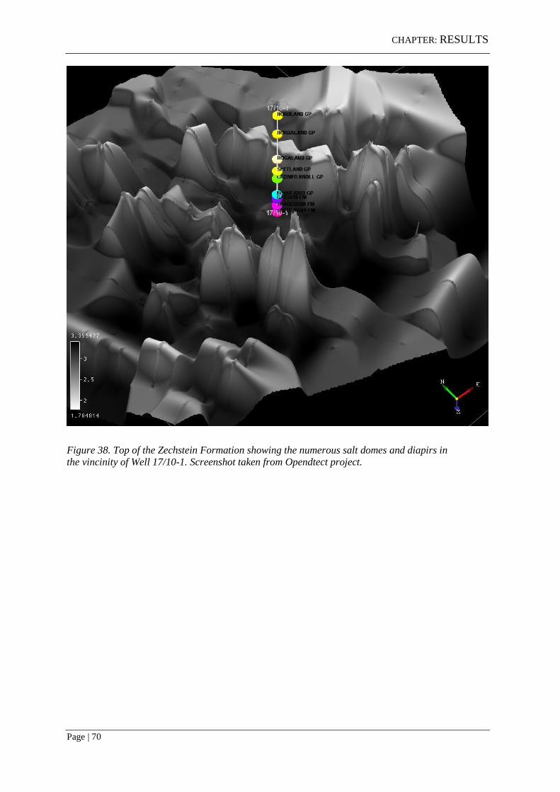
Page | 70
Figure 38. Top of the Zechstein Formation showing the numerous salt domes and diapirs in
the vincinity of Well 17/10-1. Screenshot taken from Opendtect project.
CHAPTER: RESULTS
Page | 71
Figure 39. The Permian Zechstein Formation (greyscale horizon) intruding the overlying
Gassum Formation (coloured horizon).

CHAPTER: DISCUSSION
Page | 72
7. DISCUSSION

CHAPTER: DISCUSSION
Page | 73
7.1 Discussion
An attractive option for the Sandnes / Bryne reservoir is the possibility of subsidizing a
potential storage operation with oil production utilizing the Enhanced Oil Recovery (EOR)
method. The reservoir was explored and tested for oil at the beginning of the eighties but
was considered uneconomic and unlikely to be developed. However, if the production of the
oil was in conjunction with CO2 storage, the prospect may well become economic.
From the geological well prognosis for well 18/10-1, it was noted that “the seismic character
of the Jurassic sandstone does not vary from the 17/12-1 to 18/10-1”. 17/12-1 is the
BREAM discovery, which is in the planning phase and classified as Resource Class 4F.
Therefore, it is reasonable to assume that the favourable reservoir properties could be
extrapolated to the well 18/10-1 prospect examined as part of this project.
It is also noted that the depth of the Gassum Formation reservoir in the 17/10-1 prospect is
deeper than the depth range recommended by NPD in the CO2 Atlas. Reservoirs deeper than
2500m are classified with a low score.
7.2 Limitations of this study
The nature of this study means that there is much estimation involved throughout the
process. The estimation of porosity for example doesn’t take into account the loss of porosity
due to cementation and diagenetic alteration of minerals such as quartz and kaolinite.
Another important part of the evaluation process is studying flow behaviour of target
reservoirs. Using computer simulations for modelling flow behaviour is an aspect of a
potential CO2 storage site that needs to be considered in order to understand how the
injected CO2 will behave 100 years, 1000 years 100000 years after injection as this is hoped
to be long term / permanent storage of the CO2.
7.3 Salt structures
Due to the highly pervasive nature of the salt bodies and the effect of salt tectonics in both
the Norwegian-Danish Basin and the Egersund Basin, huge regional CO2 reservoirs like the

CHAPTER: DISCUSSION
Page | 74
Utsira Formation being used by the Sleipner Project are not possible or at least too difficult
to study and predict their behaviour. It is much more likely that there is the possibility of
numerous more localised reservoirs being contained by these salt bodies. Examples of the
various salt body forms are illustrated in the diagram below (Figure 40).
Figure 40. Various forms of salt bodies. (GEO4240 lecture slides).

CHAPTER: CONCLUSION
Page | 75
8. CONCLUSION

CHAPTER: CONCLUSION
Page | 76
The Gassum Formation in the 17/10-1 prospect has moderate potential as a reservoir
for the geological storage of CO2. Using the NPD’s criteria for assessing potential
CO2 storage reservoirs, the Gassum formation could neither be classed as having
high potential or low potential, but rather falls somewhere in between. The depth of
the reservoir is of most concern as it falls outside the optimal range of between 800m
to 2500m. It is likely that there has been significant porosity reduction due to the
burial depth as well as calcite cementation.
It is unlikely that any reservoirs of sufficient capacity exist in the study area to
warrant investment on the scale needed, or to store the volumes of CO2 that could
conceivably make an impact on anthropogenic CO2 emissions. The 17/10-1 prospect
was calculated to have a storage capacity of between 750 – 850 Mt of CO2, while the
18/10-1 prospect had a much smaller storage capacity at approximately 35 Mt of
CO2. This was due to the much smaller area of the reservoir as well as being
approximately half the thickness of the 17/10-1 prospect. By comparison, the Utsira
Formation being used as a CO2 reservoir as part of the Sleipner Project has a storage
capacity of approximately 1-10 Gt of CO2.
Based on the wells analysed as part of this study, it is unlikely there is any suitable
reservoirs in the Middle Jurassic sands of the Vestland Group or Upper Triassic
sands in the Gassum Formation or Skagerrak Formation. Porosity and permeability
results calculated from well data are mostly poor with slightly more positive results
obtained from the wells 18/10-1 and 17/10-1.

CHAPTER: CONCLUSION
Page | 77
Results indicate there is limited potential for CO2 storage in the study area but more
detailed work needs to be done for this to be confirmed. Reservoir properties of the
wells analysed were poor, and the halokinesis, while creating potential plays, also
complicates the structure of the area. This makes it difficult to determine whether
reservoirs are connected and makes seismic interpretation harder as the image quality
deteriorates closer to the salt bodies.

CHAPTER: CONCLUSION
Page | 78

CHAPTER: REFERENCES
Page | 79
9. REFERENCES

CHAPTER: REFERENCES
Page | 80
Akervoll, I. and Eirik Bergmo, P., 2010. CO2 EOR From Representative North Sea Oil
Reservoirs, Sintef. SPE International Conference on CO2 Capture, Storage, and Utilization.
New Orleans, Louisiana, USA. DOI 10.2118/139765-MS.
Björnsson, S. 1991. Imaging and understanding the lithosphere of Scandinavia and Iceland
papers from a Nordic Symposium, S.l., Science Direct.
Brekke, H., Sjulstad, H. I., Magnus, C. and Williams, R. W. 2001. Sedimentary
environments offshore Norway – an overview. In: Martinsen, O. J. and Dreyer, T. (eds.)
Sedimentary environments offshore Norway – Palaeozoic to Recent. Norwegian Petroleum
Society (NPF) Special Publication; No 10.
Chadwick, R A, Arts, R, Bernstone, C, May, F, Thibeau, S, and Zweigel, P. 2008. Best
practice for the storage of CO2 in saline aquifers. Keyworth, Nottingham: British Geological
Survey Occasional Publication No. 14.
Chandra, T. 2008. Permeability estimation using flow zone indicator from well log data. 7th
International Conference & Exposition on Petroleum Geophysics. Hyderabad.
Cope, J. C. W., Ingham, J. K. and Rawson, P. F., (Ed) 1992. Atlas of Palaeogeography and
Lithofacies. The Geological Society Memoir No. 13.
CO2CRC, 2008. Storage Capacity Estimation, Site Selection and Characterisation for CO2
Storage Projects. Cooperative Research Centre for Greenhouse Gas Technologies, Canberra.
CO2CRC. Report No. RPT08-1001. 52pp.
Deegan, C. E. and Scull, B. J. (compilers) 1977. A standard lithostratigraphic nomenclature
for the Central and Northern North Sea. UK Institute of Geological Sciences, Report 77/25.
The Norwegian Petroleum Directorate, NPD-Bulletin No. 1, 36 pp.
Doveton, J. H. 1986. Log analysis of subsurface geology. New York: Wiley Interscience.
pp273.
Doveton, J. H., 2001. All Models are Wrong, but Some Models are Useful: "Solving" the
Simandoux Equation. From Session J of the International Association for Mathematical
Geology Conference, 2001, Cancun, Mexico.
IEA Greenhouse Gas R&D Programme, 2008. Geologic Storage of Carbon Dioxide: Staying
Safely Underground. International Energy Agency (IEA).
Intergovernmental Panel on Climate Change: IPCC Special Report on Carbon dioxide
Capture and Storage (CCS). Chapter 5 Underground Geological Storage.
Flett et al., 2008. Gorgon Project: Subsurface Evaluation of Carbon Dioxide Disposal under
Barrow Island. Society of Petroleum Engineers (SPE).
Fredriksen, S., Nielsen, S.B., Balling, N. 2001. A numerical dynamic model for the
Norwegian– Danish Basin, Tectonophysics, 343, 165‐183.
CHAPTER: REFERENCES
Page | 81
Gabrielsen, R.H., Faerseth, R., Steel, R. J., Idil, S., Kløvjan, O. S. 1990. Architectural styles
of basin fill in the northern Vking Graben. In: D.J. Blundell and A. D. Gibbs (eds.)
Tectonic evolution of the North Sea rifts. New York, Oxford University Press,
InternationalLithosphere Program Publication, 181, 158‐179.
Gabrielsen, R. H., Faleide, J. I., Pascal, C., Braathen, A., Nystuen, J. P., Etzelmuller, B. &
O'Donnell, S. 2010. Latest Caledonian to Present tectonomorphological development of
southern Norway. Marine and Petroleum Geology, 27, 709-723.
Glennie, K. W. and Underhill, J. R., 2009. Origin, Development and Evolution of Structural
Styles, in Petroleum Geology of the North Sea: Basic Concepts and Recent Advances,
Fourth Edition (ed K. W. Glennie), Blackwell Science Ltd, Oxford, UK. doi:
10.1002/9781444313413.ch2
Heeremans, M. and Faleide, J.I. 2004. Late Carboniferous - Permian tectonics and magmatic
activity in the Skagerrak, Kattegat and the North Sea. In: Wilson, M., Neumann, E.-R.,
Davies, G.R., Timmerman, M.J., Heeremans, M., and Larsen, B.T. (eds) Permo-
Carboniferous Magmatism and Rifting in Europe. Geological Society, London, Special
Publications, 223, 157-176.
Hermanrud, C., Eggen, S., Jacobsen, Carlsen, T., E. M. and Pallesen, S. 1990. On the
accuracy of modelling hydrocarbon generation and migration: The Egersund Basin oil find,
Norway. Advances in Organic Geochemistry. Vol. 16, Nos 1-3, pp. 389-399.
Hospers, J., Rathore, J. S., Jianhua, F., Finnstrom, E. G., and Holthe, J. 1988. Salt tectonics
in the Norwegian-Danish Basin. Tectonophysics, 149, 35-60. Elsevier Science Publishers
B.V., Amsterdam.
Hospers, J. and Holthe, J., 1984. Growth of salt-induced structures in the Norwegian-Danish
Basin. Tectonophysics, 107, 81-104 81. Elsevier Science Publishers B.V., Amsterdam.
Kaasschieter, J.P.H.; Reijers, T.J.A. (Eds.), 1982. Petroleum Geology of the Southeastern
North Sea and the Adjacent Onshore Areas.
Lyngsie, S.B., Thybo, H., Rasmussen, T.M., 2006. Regional geological and tectonic
structures of the North Sea area from potential field modelling. Tectonophysics 413, 147–
170, Elsevier.
Martins-neto, M. A. & Catuneanu, O. 2010. Rift sequence stratigraphy. Marine and
Petroleum Geology, 27, 247-253.
Michelsen, O. & Nielsen, L. H. 1993. Structural development of the Fennoscandian Border
Zone, offshore Denmark. Marine and Petroleum Geology, 10, 124-134.
Muir-Wood, R., 1987. Major fault systems on the Norwegian Continental Shelf. In: Løken,
T. (eds.) Earthquake loading on the Norwegian Continental Shelf – ELOCS Report 1-4.
Norwegian Geotechnical Institute.
CHAPTER: REFERENCES
Page | 82
Nielsen, L.H., Weibel, R., Kristensen, L., Dybkjaer, K., Japsen, P., Olivarius, M., Bidstrup,
T., Mathiesen, A., 2011. Contributions to predictions of stratigraphy and reservoir properties
in Eastern Norwegian-Danish Basin. Geological Survey of Greenland and Denmark.
Norwegian Petroleum Directorate. 2011. CO2 Storage Atlas: Norwegian North Sea.
Norwegian Petroleum Directorate, 2012. http://npd.no/en
Norwegian Petroleum Directorate, 2012. Fact Pages. http://factpages.npd.no/factpages
Olsen, R. C. 1979. Lithology Well 17/10-1. NPD Paper No. 21. Norwegian Petroleum
Directorate, Stavanger.
Pegrum, R. M. 1984. The extension of the Tornquist Zone in the Norwegian North Sea.
Geologiska Föreningen i Stockholm Förhandlingar, 106, 394-395.
Sørensen, S. & Tangen, O. H. 1995. Exploration trends in marginal basins from Skagerrak to
Stord. In: hanslien, S. (ed.) Norwegian Petroleum Society Special Publications. Elsevier.
Vangkilde-Pedersen, T. 2009. Aquifer capacity estimation. GeoCapacity results and the
future of geological storage of CO2. EU GeoCapacity open final conference held in
Copenhagen, Denmark.
Vollset, J. and Dore, A. G. (Ed.), 1984. A revised Triassic and Jurassic lithostratigraphic
nomenclature for the Norwegian North Sea. NPD Bulletin No 3. Norwegian Petroleum
Directorate
Ziegler, P.A. 1990. Geological atlas of Western and Central Europe. Shell International
Petroleum Maatschappij B.V., Geological Society, Bath.


