GEOMETRIC METHODS FOR IMAGE REGISTRATION AND ANALYSIS by Anand Arvind Joshi A Dissertation Presented to the FACULTY OF THE GRADUATE SCHOOL UNIVERSITY OF SOUTHERN CALIFORNIA In Partial Fulfillment of the Requirements for the Degree DOCTOR OF PHILOSOPHY (ELECTRICAL ENGINEERING) August 2008 Copyright 2008 Anand Arvind Joshi
Transcript
GEOMETRIC METHODS FOR IMAGE REGISTRATION AND ANALYSIS
by
Anand Arvind Joshi
A Dissertation Presented to theFACULTY OF THE GRADUATE SCHOOL
UNIVERSITY OF SOUTHERN CALIFORNIAIn Partial Fulfillment of the
Requirements for the DegreeDOCTOR OF PHILOSOPHY
(ELECTRICAL ENGINEERING)
August 2008
Copyright 2008 Anand Arvind Joshi
Dedication
I dedicate this thesis to my parents Arvind and Suvarna Joshi.
ii
Acknowledgments
I would like to express my deepest respect and gratitude to myadvisor, Prof. Richard
Leahy. His contribution has been invaluable; he supported me financially throughout
my graduate studies in USC, guided me in selecting and solving research problems,
introduced me to distinguished researchers and scientists, provided me a friendly and
welcome environment, gave me freedom to select my own research directions and let
me enjoy long holidays. He is a great mentor and a source of inspiration for me, and
it has really been an honor working with him. I also wish to thank the members of my
guidance committee: Dr. Krishna Nayak and Dr. Francis Bonahon for their sugges-
tions and valuable feedback. My appreciations go to Dr. David Shattuck and Dr. Paul
Thompson at the University of California, Los Angeles for many fruitful collaborations
and discussions. I could not have selected better colleagues than Dr. Abhijit Chaudhari,
Sangeetha Somayajula, Sanghee Cho, Joyita Dutta, Dr. Sangtae Ahn, Dr. Quanzheng
Li and Dr. Dimitrios Pantazis. We have spend quality time together, discussing research
problems as well as life experiences. I must also mention that Abhijit, Quanzheng and
Dimitrios motivated me from time to time to look for researchproblems. I also would
like to express my gratitude to Dr. Ilya Eckstein for fruitful collaborations.
In the University of Southern California I have enjoyed the cozy and warm environ-
ment of an excellent research lab. I want to thank its members: Sangtae Ahn, Abhijit
2.2 The figure shows the cortical surface and its map to a square. The corpuscallosum is constrained to lie on the boundary of the square.. . . . . . 9
2.3 Thep-harmonic maps of the left hemisphere of an individual cortex. . . 10
2.4 The figure shows smoothed histograms for angle distortion and areadistortion respectively. In the angle distortion plot, angle distortionincreases with the value ofp. In the area distortion plot, the distortionsfor p=4,6,8 are less than that forp=2 and most of the points have smallangle distortion only. However there is no observable trendfor the valueof p in either case. . . . . . . . . . . . . . . . . . . . . . . . . . . . . . 12
3.1 (a) A cortical surface with hand labeled sulci; (b) A flat map of thetwo cortical surface. The arrows show connectivity at points along theboundary of the square. Due to the spherical topology of the corticalsurface, we can assign to it a coordinate system that allows us to computepartial derivatives across the interhemispheric fissure. (c) Chessboardtexture mapped to the surface using the square maps. . . . . . . .. . . 15
3.2 (upper) The figure shows the warping field computed on the surface.The deformation field is smoothly varying. This is achieved because thebending energy regularization was performed in the intrinsic geometryof the surface. The color indicates the magnitude of the deformation.(lower) The thin-plate spline deformation field applied to aregular gridrepresenting left and right hemispheres. . . . . . . . . . . . . . . .. . 22
vii
3.3 Alignment of the sulcal landmarks: 6 brains are registered to a com-mon cortical surface using theirp-harmonic maps in the plane. Theyare approximately aligned by thep-harmonic maps justifying our smalldeformation linear model (thin plate bending energy model)which isused for landmark alignment. After applying the covariant TPS defor-mation field to the surface parameterization, we can see thatthe sulcishow better alignment. . . . . . . . . . . . . . . . . . . . . . . . . . . 26
3.4 (a),(b) The two cortical surfaces with hand labeled sulci as colored curves;(c),(d) flat maps of a single hemisphere for the two brains without thesulcal alignment constraint; (e) overlay of sulcal curves on the flat mapswithout alignment; (f),(g) flat maps with sulcal alignment;(h) overlayof sulcal curves on the flat maps with alignment. . . . . . . . . . . .. . 30
3.5 RMS error and percentage overlap in the flattened map as a function ofσ. 33
3.6 Mapping of sulcal landmarks from 5 subjects to the atlas brain (left)without and (right) with the sulcal alignment constraint. .. . . . . . . . 34
3.7 The complete set of candidate sulcal curves from which weselect anoptimal subset for constrained cortical registration . . . .. . . . . . . . 37
3.8 (a) Registration of two cortical surfaces based on the flat mapping method;(b) Parcellation of the cortex into regions surrounding thetraced sulci;(c) Registration error for two corresponding sulci whereen(s) are sam-ples of the registration error. . . . . . . . . . . . . . . . . . . . . . . . 38
3.9 Sample covariance matrices for the x, y, and z componentsof the regis-tration error, represented as color coded images. . . . . . . . .. . . . . 42
3.10 Optimal subsets of sulci for cortical registration. Each row gives theindices of the optimal subset of sulci that minimize the registration erroragainst all other combinations with equal number of constrained curves(also see Fig. 3.7). The three right columns show that the estimated(est.) error is close to the calculated actual (act.) error when actual reg-istrations with the same constrained curves are performed.Our methodpredicts the registration error both for the training (trn)and the testing(tst) set of brains. . . . . . . . . . . . . . . . . . . . . . . . . . . . . . 43
3.12 Top row: subjective selection of 6 curves, with preference on long sulcidistant from each other that are expected to minimize cortical registra-tion error; bottom row: optimal sulcal set with the 6 curves selected byour method. . . . . . . . . . . . . . . . . . . . . . . . . . . . . . . . . 46
4.1 The impulse response of the isotropic smoothing filters are displayed inthe parameter space and on the surface [JSTL05]. It can be seen thatwhen the surface metric is used to compute the Laplace-Beltrami, theimpulse response kernel is not isotropic in the parameter space, howeverit is isotropic on the surface. . . . . . . . . . . . . . . . . . . . . . . . 58
4.2 left: The mean curvature of the cortical surface plottedon a smoothedrepresentation (for improved visualization of curvature in sulcal folds;right: The mean curvature plotted in 2D parameter space for asinglecortical hemisphere. Isotropic diffusion blurs the regions as well as theedges separating them while while anisotropic diffusion reduces noisewhile preserving edges. . . . . . . . . . . . . . . . . . . . . . . . . . . 59
4.3 The figures shows the heat kernels estimated to fit the two datasets forMEG somatosensory data. For each of the datasets the estimated pdf isdisplayed in the parameter space and on the cortical surface. . . . . . . 64
4.4 The classifier: Red and Blue regions shows the two decision regions . . 64
5.1 Cortical surface alignment after using AIR software forintensity basedvolumetric alignment using a 168 parameter5th order polynomial. Notethat although the overall morphology is similar between thebrains, thetwo cortical surfaces do not align well. . . . . . . . . . . . . . . . . .. 70
5.2 Illustration of our general framework for surface-constrained volumeregistration. We first compute the mapv from brain manifold(N, I)to the unit ball to form manifold(N, h). We then compute a mapu frombrain (M, I) to (N, h). The final harmonic map from(M, I) to (N, I)is then given byu = v−1 ◦ u. . . . . . . . . . . . . . . . . . . . . . . . 74
ix
5.3 Initialization for harmonic mapping fromM to N . First we gener-ate flat square maps of the two brains, one for each hemisphere, withpre-aligned sulci. The squares corresponding to each hemispheres aremapped to a disk and the disks are projected onto the unit sphere. Wethen generate a volumetric maps from each of the brains to theunit ball.Since all these maps are bijective, the resulting map results in a bijectivepoint correspondence between the two brains. However, thiscorrespon-dence is not optimal with respect to the harmonic energy of maps fromthe first brain to the second, but is used as an initializationfor minimiza-tion of (5.6). . . . . . . . . . . . . . . . . . . . . . . . . . . . . . . . . 76
5.4 Illustration of the deformation induced with respect tothe Euclideancoordinates by mapping to the unit ball. Shown are iso-surfaces corre-sponding to the Euclidean coordinates for different radii in the unit ball.Distortions become increasingly pronounced towards the outer edge ofthe sphere where the entire convoluted cortical surface is mapped to thesurface of the ball. . . . . . . . . . . . . . . . . . . . . . . . . . . . . 77
5.5 Schematic of the intensity alignment procedure. Once harmonic mapsuM anduN are computed, we refine these with intensity driven warpswM andwN while imposing constraints so that the final deformationsare inverse consistent. . . . . . . . . . . . . . . . . . . . . . . . . . . . 82
5.6 Illustration of the effects of the two stages of volumetric matching isshown by applying the deformations to a regular mesh representing oneslice. Since the deformation is in 3D, the third in-paper value is repre-sented by color. (a) Regular mesh representing one slice in the subject;(b) the regular mesh warped by the harmonic mapping which matchesthe subject cortical surface to the template cortical surface. Note thatdeformation is largest near the surface since the harmonic map is con-strained only by the cortical surface; (c) Regular mesh representing oneslice in the harmonically warped subject; (d) the intensity-based refine-ment now refines the deformation of the template to improve the matchbetween subcortical structures. In this case the deformation is con-strained to zero at the boundary and are confined to the interior of thevolume. . . . . . . . . . . . . . . . . . . . . . . . . . . . . . . . . . . 85
5.7 Examples of direct mapping approach. (a) Original subject volume; (b)original template; (c) registration of subject to templateusing surfaceconstrained harmonic mapping, note that the surface matches that of thetemplate; (d) intensity-based refinement of the harmonic map of subjectto template to complete registration procedure . . . . . . . . . .. . . . 88
x
5.8 Volumetric registration using direct mapping approach: (a) Illustrationof the extrapolation of the surface mapping to the 3D volume by har-monic mapping. The pairs of surfaces are shown in red and green. Thedeformation field is represented by placing a regular grid inthe centralcoronal slice of the brain and deforming it according to the harmonicmap. The projection of this deformation onto a 2D plane is shown withthe in-plane value encoded according to the adjacent color bar. (b) Theresult of harmonic mapping and linear elastic refinement of the sub-ject brain to the template brain. Note that the inner and outer corticalsurfaces, by constraint, are exactly matched. The linear elastic refine-ment produces an approximate match between subcortical structures.The deformation field here shows the result of cortically constrainedintensity-driven refinement. Note that the deformations are zero at theboundary and nonzero in the vicinity of the ventricles, thalamus andother subcortical structures. . . . . . . . . . . . . . . . . . . . . . . . .90
5.9 Examples of surface constrained volumetric registration. (a) Originalsubject volume; (b) template; (c) registration of subject to templateusing surface constrained harmonic mapping, note that the cortical sur-face matches that of the template; (d) intensity-based refinement of theharmonic map of subject to template . . . . . . . . . . . . . . . . . . . 91
6.1 Geometric framework for registration and analysis . . . .. . . . . . . . 95
xi
Abstract
Registration and analysis of neuro-imaging data presents achallenging problem due to
the complex folding patterns in the human brain. Specifically, the cortical surface of the
human brain can be modeled as a highly convoluted 2D surface.Since it is non-flat, the
non-Euclidean geometry of the cortex needs to be accounted for while performing reg-
istration and subsequent signal processing of anatomical and functional signals on the
cortex. Techniques from differential geometry offer a powerful set of tools to deal with
the convoluted nature of the cortex. We present a method based on p-harmonic mapping
for performing cortical surface parameterization. A 2D coordinate system induced by
the flat mapping is then used to compute the surface metric anddiscretize derivatives
in the surface geometry. For performing inter-subject cortical registration based on sul-
cal landmarks, we generalize thin-plate splines to non-flatsurfaces by using covariant
derivatives. We also present an FEM based method for simultaneous parameterization
and registration of sulcal landmarks based on elastic energy minimization. The man-
ual effort required for selecting the sulcal landmarks can be minimized if we choose
an optimal set of such landmarks. We present a method for optimally selecting a sub-
set of any size from a set of candidate sulcal landmarks and also predict the associated
registration error for that subset using conditional distributions. Surface signals from
individual brains can be brought to a common atlas surface byusing these surface based
registration techniques.
xii
Isotropic and anisotropic diffusion filtering methods are formulated for processing
of the cortical data. This is performed by using parameterization-based methods which
use covariant diffusion operators in the flat space. When thesurface data is a point-set
on the cortex, we propose a method to quantify its mean and variance with respect to
the surface geometry.
The registration techniques presented for surface alignment are extended to volumes
to perform full surface and volume registration. This is done by using volumetric har-
monic mappings that extend the surface point correspondence to the cortical brain vol-
ume. Finally, the volumetric registration is refined by using inverse-consistent linear
elastic intensity registration. This set of methods presents a unified framework for reg-
istration and analysis of brain signals for inter-subject neuroanatomical studies.
xiii
Chapter 1
Introduction
Brain is home to our mind and personality. It houses our cherished memories and future
hopes. It orchestrates the symphony of consciousness that gives us purpose and passion,
motion and emotion. Understanding the workings of human mind can only be achieved
if we understand the structure and function of the human brain.
The outer part of the brain comprises of grey matter which is internally supported
by white matter. The two hemispheres of the brain are separated by the central fissure
and connect to each other at the corpus callosum. Cerebellumis found at the posterior-
inferior part of the brain. Cerebral cortex or simply cortexis the outermost layer of the
cerebrum and is the place where most of the neuronal activations take place. The human
cerebral cortex is 2-4 mm thick and plays a central role in many complex brain functions
including memory, attention, perceptual awareness and language. Due to the relatively
small thickness of the cortex, it can be modeled as a 2D highlyconvoluted surface
with more than two third buried in the grooves, calledsulci. The sulcal folding pattern
varies across individuals, however, some of the major sulciare seen across individuals
[OKA90]. It is known that the sulci are related to the function of the brain and therefore
inter-subject alignment of the cortex should be carried outwith the constraint that these
sulci are aligned.
Medical imaging modalities acquire various anatomical (CT, MR, etc.) and func-
tional (PET, EEG, MEG, etc.) neuro-imaging data. Intersubject analysis of this data
allows us to study group differences and similarities. The anatomical variability across
individuals needs to be normalized before such a study can becarried out. Medical
1
Figure 1.1: The cortical surface of the human brain depictedon a MR data (top row)and rendered as a surface (bottom row).
image registration performs this normalization by aligning the coordinate systems of
the various medical images to register them to a common template or atlas. One of the
most challenging problems in image registration is the alignment of human brains.
Registration of surface models of the cerebral cortex has important applications in
inter-subject studies of neuroanatomical data for mappingand analyzing progression of
disorders such as Alzheimer’s disease [TMV+01] and studying growth patterns in devel-
oping human brains [TMT00, GGL+04]. Investigators have studied several anatomical
and functional aspects of the human brain such as genetic influences [THdZ+02] and
the influence of medication and drugs abuse on the structure and function of the brain
[NB97, Cha01]. Inter-subject analysis, or intra-subject analysis over a period of time of
such data, present difficult problems due to the inter-subject variability and convoluted
geometry of the cortical surface. Since most neural and metabolic activity takes place
in the cortex, and because the thickness of the cortex is small relative to the resolution
2
of most functional imaging techniques, it is plausible to model the cortex as a surface
rather than as a volume.
Since the cortex is non-flat, the non-euclidean geometry of the cortex needs to be
accounted for while doing registration and subsequent signal processing of anatomical
and functional signals on the cortex. In this report we propose a surface parameterization
method which computes a 2D coordinate system on the cortex. We usep-harmonic map-
ping of the cortex toR2 to assign 2D coordinates to the surface points. This coordinate
system is then used to compute the associated surface metricfor the assigned coordi-
nates which are then used to discretize derivatives in the surface geometry. In order to
bring several brain surfaces in a common template space, we present two surface reg-
istration techniques to find a point to point correspondencebetween the two surfaces.
The first technique involvesp-harmonic mapping of the cortex to a plane and then repa-
rameterization with thin-plate bending energy as a regularizing function. Alternatively,
the second technique incorporates sulcal landmark matching in the parameterization
method itself. This is done by using a more general elastic model for parameteriza-
tion. The point correspondence set by surface registrationcan be used to bring surface
functional signals such as MEG dipoles or neuronal activations, fMRI and anatomical
signals such as cortical thickness from individual brains to a common atlas surface.
Isotropic and anisotropic diffusion filtering methods are formulated for different kinds
of smoothing of such cortical data. When the surface data is apoint-set on the cor-
tex, we propose a method to quantify its mean and variance with respect to the surface
geometry. The registration technique presented for surface alignment is then extended
to volumes to perform full surface and volume registration using harmonic mappings.
Inverse-consistent elastic intensity registration is then used to further improve the volu-
metric alignment. Various validation techniques were usedto assess the performance of
3
the above tools and to compare them with existing methods as presented in subsequent
chapters.
4
Chapter 2
Cortical Surface Parameterization
The surface area of the cerebral cortex is approximately1570 cm2 [HSB+00]. 60-70% of
the surface area is buried in the folds and creases (sulci). There is considerable variabil-
ity and individual differences in the size, location and extent of the sulci and gyri across
human subjects. Bringing multiple brain surfaces into a common coordinate system is
helpful in studying variability of these sulcal patterns across subjects, for integrating and
averaging functional data across subjects, and in studyingpatterns in cortical develop-
ment over time. Since the cortex can be modeled as a convoluted sheet with the topology
of a sphere, it is natural to parameterize it using sphericalcoordinates[FSTD98]. Eck
et al.[EDD+95] and Kanai et al.[KSK98b] model a triangulated surface asa configura-
tion of springs with one spring placed along each edge of eachtriangle. The resulting
energy functional, theharmonic energy,is shown to be a quadratic form and is mini-
mized using gradient descent to transform the surface into aplanar disk. Desbrun et
al.[DMA02] propose a parameterization technique which uses thecot of angles in the
given triangulation. The resulting energy functional (Tuette energy) is argued to be a
measure of angle distortion and a new parameterization is obtained by minimizing it.
Haker et al.[AHTK99] presented a method for conformally mapping the cortical surface
to a sphere. Their method uses the Laplace-Beltrami operator and the fact that for a con-
formal map, the Laplace-Beltrami of the parameterization function is zero everywhere
on the surface. Though these methods ensure a perfectly conformal map, the stereo-
graphic projections involved can introduce a large amount of length and area distortion.
5
Figure 2.1: Sulcal Tracing Tools
Circle packing is introduced as a parameterization method in [HSB+00]. Analytic sur-
faces can be approximated by circle packing, but for generalsurfaces, the surface pack-
ing method considers only the connectivity and not geometry[WGH+05]. Fischl et al.
used mechanical models to simulate an inflation of the cortical surface to produce an
inflated surface and a spherical map [FSTD98].
We proposed a parameterization technique for the cortical surface based onp-
harmonic energyminimization [JLTS04]. Angle and area distortion metrics were com-
puted to evaluate the performance of this flattening procedure.
2.1 Parameterization and the Coordinate System
In this section, we describe our method to parameterize a triangulated surface mesh. In
the context of our work, this mesh will typically represent the surface of the cerebral
cortex; thus we will refer to this mesh model as the cortical surface. We use ourp-
harmonic mapping technique [JLTS04] for parameterization. The parameterization can
be viewed as an assignment of complex numbers or vectors inR2 to each vertex in the
6
triangulated surface and the assignment is performed in such a way that the resulting
p-harmonic energy is minimized. LetS be a surface with boundary. We defineφ :
S → R2 to be a function such that thep-harmonic energy given byEs =
∫‖∇φ‖p dS
is minimized. We impose constraints on this minimization byfixing the location of the
inter-hemispheric fissure so that it is mapped to a unit square. We rewrite the energy
functional as the sum of two energy functionalsφ = [α, β]′, one for each coordinate,
such that the corresponding arguments are scalars,
Es =
∫
‖∇φ‖p dS, p ∈ (1,∞)
This minimization can be performed by minimizations over two real-valued functions.
Discretization is done using finite elements. We make the assumption that both of them
are piecewise linear. Letα be a piecewise linear real-valued scalar function defined over
the surface, andαi is α restricted to trianglei. Sinceαi is linear on theith triangle we
can write,
αi(x, y) = ai0 + ai1x+ ai2y (2.1)
The three coefficients can be determined if values of the function α are known at the
three vertices of the triangle. These equations can be written in matrix form as
1 xi1 yi1
1 xi2 yi2
1 xi3 yi3
︸ ︷︷ ︸
Di
ai0
ai1
ai2
=
αi(x1, y1)
αi(x2, y2)
αi(x3, y3)
(2.2)
7
The coefficientsai0, ai1 andai2 can be obtained by inverting the3× 3 matrix. From (2.1)
and by inverting the matrix in (2.2), we obtain
−−→∇αi =
ai1
ai2
=1
|Di|
yi2 − yi1 yi3 − yi1 yi1 − yi2
xi1 − xi2 xi1 − xi3 xi2 − xi1
︸ ︷︷ ︸
Bi
αi(x1, y1)
αi(x2, y2)
αi(x3, y3)
︸ ︷︷ ︸
Γi
−−→∇αi =
1
2AiBiΓi
We use the fact that for any triangle,|Di| = 2Ai whereAi is the area of the triangle.
Sinceαi is piecewise linear, its gradient is constant over each trianglei, so that:
∫
‖∇α‖p dS =∑
i
‖∇α‖pAi
where the sum is over all triangles. Therefore,
arg minα
∫
‖∇α‖p dS = arg minΓ
∑
i
∥∥M iΓi
∥∥p
= arg minΓ
‖MΓ‖p
whereM i = 1(Ai)(p−1)/pB
i, M is composed using coefficients ofBi andΓ is a vector
with coefficientsα for each vertex. The vectorMΓ can be split into two parts: free
vertices and constrained vertices. Values ofα at constrained vertices are known.
arg minα
∫
‖∇α‖p dS = arg minΓf
‖MfΓf +McΓc‖p
8
Figure 2.2: The figure shows the cortical surface and its map to a square. The corpuscallosum is constrained to lie on the boundary of the square.
whereMf , Γf andMc,Γc are free and constrained parts of theM andΓ matrices.
This results in an unconstrained minimization problem. Thefact that matrixMf
is sparse allows us to use the computationally efficient conjugate gradient method for
obtaining the solution. The Jacobi preconditioner reducesthe execution time consider-
ably. The resulting maps are known to be bijections because the target domain is convex
and flat [ES64, Ham75, FR02]. Using this scheme, we map each cortical hemisphere
onto a unit square by constraining the inter-hemispheric fissure to lie on the boundary
of the square.
2.1.1 Validation ofp-harmonic mappings
In this section we present our method of evaluating the performance of thep-harmonic
mappings described in section 2.1. We start by extracting a high-resolution trian-
gulated cerebral cortical surface model for each brain. Each brain surface is rep-
resented by approximately200, 000 triangles. The BrainSuite software we use for
9
(a) p = 2 (b) p = 4
(c) p = 6 (d) p = 8
Figure 2.3: Thep-harmonic maps of the left hemisphere of an individual cortex.
extraction also labels and separates the two cortical hemispheres and delineates the
closed contour representing the inter-hemispheric fissurethat separates the two hemi-
spheres. We then parameterize the contour according its length and constrain it to
lie on the boundary of the unit square. The mapping describedin section 2.1 is then
computed by minimizing thep-harmonic functional by conjugate gradient with Jacobi
preconditioner [Smi85]. The minimization is very fast compared to other methods
[AHTK99, FSTD98, HSB+00] and takes on the order of 20 seconds on 3GHz Intel Pen-
tium 4 processor. Performing this operation for both hemispheres produces a bijective
mapping of the cortical surface to a pair of unit squares.
10
In order to explore and evaluate the performance of such mappings and their depen-
dence on the value ofp chosen, we computed these mappings forp = 2, 4, 6, 8 and used
the following metricsNangle andNarea as measures of angle and area distortions.
Nangle =√
|g11g12 + g21g22| /g (2.3)
Narea = ‖g − gavg‖ (2.4)
Nangle can be interpreted as a normalized inner product of the two columns of the
metric tensor. It is zero if the mapping preserves angles (conformal).Nangle is deviation
of the differential areadS from its mean value. We evaluate these metrics at all the
vertices and then plot their histograms for different values of p. The Fig. 2.4 shows
p-harmonic maps of the cortical surfaces for the values ofp = 2, 4, 6 and8. It can be
seen from Fig. 2.4(a) that maps forp = 4, 6, 8 have much less area distortion than the
map forp = 2. However there was no consistent trend for the values ofp. Also it can
be seen from Fig. 2.4(b) that the angle distortions are comparable for all values ofp.
From a computational point of view, though the use of covariant derivatives can make
the subsequent processing independent of the value ofp, we choosep = 4 because it
has less area distortion thanp = 2 case and hence the numerical error introduced during
the resampling of the cortical surface on a regular grid is less.
11
−0.5 0 0.5 1 1.5 2 2.5 30
0.2
0.4
0.6
0.8
1
1.2
1.4
Angle Distortion
Num
ber
of O
ccur
ance
s
P=2P=4P=6P=8
(a) Angle Distortion
0 50 100 15010
−5
10−4
10−3
10−2
Area Distortion
Num
ber
of O
ccur
ance
s
p=2p=4p=6p=8
(b) Area Distortion
Figure 2.4: The figure shows smoothed histograms for angle distortion and area distor-tion respectively. In the angle distortion plot, angle distortion increases with the valueof p. In the area distortion plot, the distortions forp=4,6,8 are less than that forp=2and most of the points have small angle distortion only. However there is no observabletrend for the value ofp in either case.
12
Chapter 3
Cortical Surface Registration
Various surface-based techniques have been developed for inter-subject registration of
two cortical models. These techniques can be used to register subject surfaces to a com-
mon atlas which in turn registers cortical data representing structure and function of
the human brain to the atlas. There are two main categories ofmethods that align the
cortex from a subject to an atlas: manual landmark based methods [JSTL07c] and auto-
matic methods based on alignment of geometric features [WCT05] or surface indices
[TRP05]. The main advantage of automatic methods is that there is no manual input
required for performing the alignment. However they may be less reliable in the sense
that they do not incorporate higher level knowledge of sulcal anatomy. While they have
been successfully applied in several settings, their accuracy may not be satisfactory for
expert neuroanatomists, particularly in the presence of the wide variation that may be
present in neuroanatomy or the image acquisition quality. Data from subjects exhibiting
abnormal cortical shape, such as individuals with Alzheimers disease, may be handled
better by manual delineation. It is likely that landmarks defined by experts, who have
been trained to make consistent decisions when faced with ambiguities that frequently
arise in the analysis of cortical geometry, will produce improved registration results. In
some cases a particular area, such as the visual cortex, may be of interest and constraints
specific to that area may provide more appropriate registration.
One class of techniques involves flattening the two corticalsurfaces to a plane
[HSB+00] or to a sphere [FSTD98] using mechanical models or variational methods and
then analyzing the data in the common flattened space. Other surface based techniques
13
work in the surface geometry itself rather than a plane or a sphere and choose to account
for the surface metric in the inter subject registration [TWMT00, THS+04, LTPH04,
MST04, WGH+05]. The advantage of such techniques is that they make the registra-
tion results independent of the intermediate flat space resulting in a more consistently
accurate registration throughout the cortex. In this chapter we present a technique that
is a generalization of the popular thin-plate spline methods fromRn to a non-Euclidean
surface, as well as a Finite Element-based technique.
We presented ourp-harmonic mapping method in Chapter 2, which maps each indi-
vidual cortical hemisphere to the unit square. Ourp-harmonic method results in a very
fast parameterization of high-resolution cortical surfaces and always results in a bijective
map. We use the resulting square maps of the cortical hemispheres to assign a coordinate
system to the cortex. We then use these coordinates to compute the metric tensor and
Christoffel symbols of the mapping. In order to register onebrain to another, we warp
coordinates of one brain with respect to another using sulcal landmarks such that the
bending energy is minimized within the true geometry of the surface. This is achieved
by solving the resulting variational problem using covariant derivatives and thus mak-
ing the warping results independent of the coordinate system. Our warping approach is
derived from the one presented in [TWMT00]. However, we use thin plate splines as
a regularizing function. This is because the availability of p-harmonic maps allows us
to have an approximate orthogonal coordinate system on the cortical surface and there-
fore we are able to decompose the deformation into two orthogonal components. Also
availability of a smooth parameterization from 3D space to unit square means that the
deformations are low dimensional in the parameter space too. Therefore we use DCT
basis functions to represent the warping field. These techniques result in a considerable
speed up and stability in the registrations. As an improvement over this method, we also
14
present a simultaneous parameterization and alignment technique as discussed further
in Sec. 3.2. We also present evaluations of these registration techniques.
Figure 3.1: (a) A cortical surface with hand labeled sulci; (b) A flat map of the two cor-tical surface. The arrows show connectivity at points alongthe boundary of the square.Due to the spherical topology of the cortical surface, we canassign to it a coordinatesystem that allows us to compute partial derivatives acrossthe interhemispheric fissure.(c) Chessboard texture mapped to the surface using the square maps.
15
3.1 Thin Plate Splines Registration in the Intrinsic
Geometry of the Cortical Surface
3.1.1 Mathematical Formulation
The parameterization method presented in Chapter 2 gives usan initial approximate
alignment of the labeled sulcal landmarks as shown in Fig. 3.3. It can be seen that the
alignment is not perfect, however the deformation requiredto align the sulci perfectly
is relatively small compared to the brain size. Therefore weuse linear models from
continuum mechanics which approximate small deformationsto regularize the required
deformation field. Here we discuss the widely used thin-plate splines, but we generalize
them to the non-Euclidean geometry of the cortical surface.Having parameterized each
of the cortical surfaces, we now align coordinate systems between one surface, which
we denote the “atlas”, and another which we call the “subject”. The alignment uses a
set of manually labeled sulci, sampled uniformly along their lengths, as a set of point
constraints [TT96b]. To compute a smooth warping fieldφ from one coordinate sys-
tem to the other we use the thin plate spline bending energy onthe subject surface as a
regularizing function. Thep-harmonic maps serve two purposes. First, they set up an
initial alignment of the features across multiple subjects. Second, they are used as our
computational space to align the cortices. However, the thin-plate spline based align-
ment uses covariant derivatives, and is therefore invariant with respect to the specific
parameterization [TMV+01].
Thin plate biharmonic splines [Boo89] are a very popular method for landmark-
based registration of 2D or 3D images. These splines are solutions of the biharmonic
equation∂4φ
∂u4+ 2
∂4φ
∂u2∂v2+∂4φ
∂v4= 0 (3.1)
16
or equivalently, they solve a variational problem that minimizes the bending energyEb
of a thin metal plate:
Eb =
∫ (∂2φ
∂x2
)2
+ 2
(∂2φ
∂x∂y
)2
+
(∂2φ
∂y2
)2
dxdy (3.2)
We minimize this bending energy subject to the point landmark constraints, imple-
mented here using a quadratic penalty function approach. Since we wish to minimize the
bending energy in the surface, we must account for the intrinsic geometry of the surface
when computing the integral. While we use the parameter space for doing the calcu-
lations required for evaluation of the bending energy, we account for the effect of the
parameterization while calculating the integral. This is achieved using covariant deriva-
tives which results in the property that given a set of homologous landmarks in some
initial alignment, the deformation is independent of the parameterization used for the
computation of the TPS deformation field. The use of covariant derivatives eliminates
the effect of the initial parameterization on the resultingwarping field.
Let x denote the 3-D position vector of a point on the cortical surface. Letu1, u2
denote the coordinates in the parameter space. The metric tensor coefficients required
in the computation are given by:
g11 =
∥∥∥∥
∂x
∂u1
∥∥∥∥
2
, (3.3)
g22 =
∥∥∥∥
∂x
∂u2
∥∥∥∥
2
, (3.4)
g12 = g21 =
⟨∂x
∂u1,∂x
∂u2
⟩
, (3.5)
g =√
g11g22 − (g12)2 (3.6)
We note that the eigenfunctions of the biharmonic operator on the surfaces are dependent
on the surface itself. Therefore we do not expand the deformations in terms of a common
17
eigenfunction basis as in [Boo89]. Instead we take a more direct approach and minimize
the integral numerically. The bending energy is minimized in the intrinsic geometry after
replacing the first and second partial derivatives in (3.2) by the corresponding covariant
derivatives. Integration over the surface can be carried out by integration in the param-
eter space while compensating with the surface metricg. The differential formds2 for
the integration in the surfaceS is related to its counterpart in the parameter space(u, v)
by ds2 = gdudv. LetS be the set of all vertices, and letSc denote the set of constrained
vertices (landmarks). Letd1j andd2
j denote theu andv displacements required at the
jth landmark,1 ≤ j ≤ N , to take it to its location in the atlas space. Cartesian ten-
sors suffice for flows in 2D or 3D Euclidean spaces. However thecortical surface is
a two dimensional non-Euclidean space and from the outset demands a full tensorial
treatment. We do this by replacing the usual partial derivatives by covariant derivatives
as done in continuum mechanics on manifolds [Kre99]. Although we want the deforma-
tion field with respect to the cortical surface to be independent of the specific choice of
parameterization, the deformation field expressed in the 2Dparameter space invariably
does depend on the initial parameterization. This propertyis desirable since it ensures
the covariance properties of the deformation vector field. Small deformations expressed
in the parameter space can be modeled as contravariant vectors [TMT00, Kre99] since,
with respect to two different parameterizationsu andu, the respective values of the
deformationsφ andφ are related byφβ
= φj ∂uβ
∂uα . In order to preserve their tensorial
nature, we need to use covariant derivatives instead of the usual partial derivatives. The
covariant derivativeφβ,σ of a contravariant tensorφβ is given by:
φβ,σ =∂φβ
∂uσ+ φκΓ β
κσ whereα, β, κ ∈ {1, 2} (3.7)
18
whereΓ βκσ denote the Christoffel symbols of the second kind [Kre99] given by:
Γ ααα =
1
2g
[
gββ∂gαα∂uα
+ g12
(∂gαα∂uβ
− 2∂g12
∂uα
)]
(3.8)
Γ βαα =
1
2g
[
gαα
(
2∂g12
∂uα− ∂gαα
∂uβ
)
− g12∂gαα∂uα
]
(3.9)
Γ βαβ = Γ β
βα =1
2g
[
gαα∂gββ∂uα
− g12∂gαα∂uβ
]
(3.10)
whereα, β ∈ {1, 2}. The first covariant derivative of a contravariant tensorφζ is a
mixed tensorφζ,β. Covariant derivativesφζ,βσ of such a tensor are given by:
φζ,βσ =∂φζ,β∂uσ
− φζ,µΓµ
βσ + φ νβ Γ ζ
νσ
whereσ, β, ζ, µ, κ ∈ {1, 2} (3.11)
The warping field(φ1, φ2) with respect to the parameter space(u, v) that minimizes
bending energy in the surface while matching the constraints is then given by:
φ1 = arg minψ1
∫
P
(
(ψ1,11)
2 + (√
2ψ1,12)
2 + (ψ1,22)
2)
gdudv,
with φ1(uj, vj) = d1j , ∀j ∈ Sc (3.12)
φ2 = arg minψ2
∫
P
(
(ψ2,11)
2 + (√
2ψ2,12)
2 + (ψ2,22)
2)
gdudv,
with φ2(uj, vj) = d2j , ∀j ∈ Sc (3.13)
The warping field(φ1, φ2) at the interhemispheric fissure is not forced to be zero as
described in the next section.
19
3.1.2 Discretization Algorithm
In order to solve (3.12) and (3.13) for the thin-plate splineregistration, we need to
discretize the integral in that equation. We use thep-harmonic square maps of the trian-
gulated tessellation of the cortical surface for defining a coordinate system. The square
maps for each hemisphere are then resampled on a regular 256x256 grid. Because the
interhemispheric fissure is fixed on the boundary of the square for each hemisphere, one
can visualize the(u, v) parameter space as two squares placed on each other and con-
nected at the boundaries of the squares. The main advantage of this space is the ease
of composing and solving various partial differential equations in discrete form since
this allows us to calculate partial derivatives across the two hemispheres and to include
explicitly the connectivity of the two cortical hemispheres in subsequent analysis. This
boundless space is then used for discretizing the partial derivatives with respect tou and
v spatial coordinates in the solution of the differential equations. For instance, assume
that f : M → R is a scalar-valued function defined on the cortical surfaceM . We
arrange its discretized representation at each vertex in the triangulation of the surface in
a vector~f = fi. In order to discretize∂f∂u
by central difference, we calculate the usual
central difference at the interior points in the squares. Onthe boundary of the squares,
we consider the connectivity relationship shown in Fig. 3.1for the neighborhood in the
central difference approximation. Using these relations,we compose a central difference
matrixDcu and obtain discretization of∂f
∂uasDc
u~f . Similarly we compose matricesDf
u,
Dbu, the forward and backward difference operators for theu coordinate, andDc
v,Dfv and
Dbv, — the central, forward and backward difference operators —for thev coordinate.
We carry out the discretization of the linear operator corresponding to the bending
energy in (3.12) and (3.13) in the following steps.
1. Parameterize the cortical surface to map it into two squares and assign to it the
coordinate system described above.
20
2. Form the forward, backward and central difference matricesDfu, D
fv , Db
u, Dbv and
Dcu, D
cv for u andv coordinates respectively.
3. Compute the surface metric coefficientsg11, g12, g21 andg22. This is accomplished
by replacing partial derivatives in (3.3), (3.4), (3.5) and(3.6) by their discrete
versions from step 1.
4. Compute the Christoffel symbols according to (3.8), (3.9) and (3.10) by replacing
partial derivatives in that equation by finite difference matrices from step 1.
5. Compute the first and second covariant derivative operators using (3.7) and (3.11).
This can be done by first computing the operator corresponding to (3.7) and then
using it to compose the operator corresponding to (3.11). Replace the partial
derivatives in their expressions by finite difference matrices from step 1 and con-
catenate them to form a covariant bending energy functionalmatrix which is used
to minimize the covariant bending energy.
3.1.3 Bending Energy Minimization
We discretized the bending energy integral in (3.12) and (3.13) in the parameter space
over a 256x256 regular grid for each hemisphere. We denote the covariant differen-
tial operator in these equations byL. As described previously, our parameter space
takes into account the neighborhood relationships betweenthe two hemispheres and thus
the covariant operatorL is discretized in such a way that derivatives at the interhemi-
spheric fissure are calculated correctly. In our current implementation our constraints are
enforced by adding a quadratic penalty term rather than the exact matching constraints
21
Figure 3.2: (upper) The figure shows the warping field computed on the surface. Thedeformation field is smoothly varying. This is achieved because the bending energyregularization was performed in the intrinsic geometry of the surface. The color indi-cates the magnitude of the deformation. (lower) The thin-plate spline deformation fieldapplied to a regular grid representing left and right hemispheres.
in (3.12) and (3.13). LetΦ = (φ1, φ2) denote the deformation field. The discretized cost
function then takes the form
Φ = arg min∑
i∈S
||√gLiΦi||2+
σ2∑
j∈Sc
||√g(LjΦj − dj)||2 (3.14)
22
The resulting least squares problem is very high-dimensional (256x256x2x2 parame-
ters), but it could be solved directly since the matrixL is sparse. However, we reduce
the dimensionality of the problem by projecting onto a subset of the discrete cosine
transform (DCT) basis functions. Provided the constraintscan be satisfied with a rel-
atively smooth deformation, this approach will work with fewer basis functions than
the original 256x256 samples in(u, v) space. LetB denotes the DCT basis matrix,
T = LB, Ψ = BTΦ andTi = LiB. The optimization problem
Φ = arg min∑
i∈S
||√gLiBBTΦi||2
+σ2∑
i∈Sc
||√gLiBBTΦi − di||2 (3.15)
reduces to:
Ψ = arg min∑
i∈S
||√gTΨ||2 + σ2∑
i∈Sc
||√gTiΨ − di||2 (3.16)
In this way, we calculate the deformations in the DCT transform space. Use of this basis
leads to a significant increase in speed. We observe that choosing a higher value of the
parameterσ will lead to more accurate alignment of the sulcal landmark points, but in
practice a very high value leads to non-bijective deformation of the coordinate space.
Due to this trade-off, we pick a value ofσ by trial and error. For certain individual
subjectsσ is decreased if the deformation field is non-bijective. The warps thus obtained
are then applied to the(u, v) coordinates of each cortical surface to coregister them to
the template. This process is illustrated in Fig. 3.2 where we show the sulci traced on
the original cortical surface and their corresponding locations in flat space. We then
show the relative locations of these sulcal features in flat space for the subject and atlas
before and after matching. Note that we use a quadratic penalty function to match the
23
landmarks so that they do not exactly align after registration. Cortical regions near the
boundary of the unit square exhibit larger metric distortion relative to the cortical surface
than do regions near the center. Since the warp bending energy is computed with respect
to the intrinsic geometry of the surface rather than flat space, we see that the warp in flat
space exhibits larger deformations near the boundaries than at the center, following the
pattern of metric distortion.
3.1.4 Validation TPS surface registration
Alignment of two cortical surfaces was performed using the intrinsic TPS method pre-
sented above. For our purpose, we used 16x16 DCT basis functions in each of theu
andv directions. We found that the resulting warps closely resembled the warping field
computed without using basis functions. The use of basis functions resulted in a run-
time of 2 min. as compared to the runtime of 2 to 3 hours in the case of computation
without using basis functions. Fig. 3.3 shows alignment of sulcal maps before and after
registration. The warping field is smooth on the cortex sincethe surface geometry was
considered during the regularization.
There is no gold standard for evaluating the performance of registration algorithms
such as the one presented here. However, there are several properties that are desirable
for any surface registration algorithm. Our method for evaluating the quality of our
registration results is based on the following properties:
1. Insensitivity to the anatomical variability between multiple subjects. Though it
is difficult to expect any automatic registration algorithmto align the anatomi-
cal features accurately, we expect a sulcus to be aligned more accurately if the
remaining sulci are used as landmarks and are forced to align.
24
2. Insensitivity to a small amount of noise in the extracted surface coordinates. The
process of extracting the cortical surface involves several stages and the results
of each stage are sensitive to various parameters. We model this variability intro-
duced during the extraction process as additive Gaussian noise in thex, y, z coor-
dinates. The warping process should be relatively insensitive to this noise and
should depend only on the global structure of the brain.
3. Insensitivity to small linear (affine) scaling of the surface coordinates. These kind
of volumetric warps can get introduced in the imaging process. Also brains from
different age groups have different sizes and registrationshould not depend on
factors such as the overall size of the brain.
The error results presented here are in terms of the root meansquared error. In order
to evaluate performance with respect to (1), we carried out aleave-one-out validation
scheme. We aligned cortices of 6 subjects with one another using 22 out of 23 labeled
sulci leaving one sulcus out of the registration each time. For each of the6C2 ∗ 23 =
345 registrations, we measured how well the sulcus that was leftout of the registration
process aligns across the subjects before and after registration. Before carrying out the
warping, there was mean squared error of 28.6 mm in the free sulcus. After aligning all
but the free sulcus, the remaining root mean squared error was 2.81 mm. For (2), we
added Gaussian noise in each of thex, y, z coordinates and register each of the brains
with the noiseless brains. In this case, since we know the correct point correspondence
between the noiseless and the noisy brains, we calculated the alignment error for the
entire surface rather than just the sulci. Before applying TPS warping, there was 40.9
mm mean squared error. After warping there was 3.58 mm alignment error. For (3) we
applied affine warps to the cortical surfaces and aligned theaffine warped surface with
the original surfaces. In this case also we calculated errorfor the entire surface as in (2).
Before warping there was 35.8 mm error which reduced to 3.18 mm error after warping.
25
(a) Alignment in the square space(b) Initial alignment in referenceatlas space
(c) Alignment in the square spaceafter covariant TPS warping
(d) Alignment in the brain atlasspace
Figure 3.3: Alignment of the sulcal landmarks: 6 brains are registered to a common cor-tical surface using theirp-harmonic maps in the plane. They are approximately alignedby thep-harmonic maps justifying our small deformation linear model (thin plate bend-ing energy model) which is used for landmark alignment. After applying the covariantTPS deformation field to the surface parameterization, we can see that the sulci showbetter alignment.
3.2 A Finite Element Method for Simultaneous Regis-
tration and Parameterization
The method presented in Sec. 3.1 is a two step procedure whichfirst maps the
two cortical surfaces to a plane and then computes a deformation vector field that
26
aligns sulcal landmarks with respect to their planar coordinates. Similar methods
were presented by various researchers which use plane, sphere or some intermedi-
ate representation of the cortex as a common space for performing the alignment
[HSB+00, BGKM98, FSTD98, TRP05, THS+04, WGH+05, JSTL05]. In our two step
procedure, in order to solve the resulting variational minimization problem, numerical
derivatives were computed by resampling the brain on a uniform grid with respect to the
parameterization. In addition to the computational cost ofresampling and interpolation,
this step results in a loss of resolution since the regular orsemi-regular grid in flat space
is not necessarily optimal for representing the brain in 3D space. In our new approach,
we incorporate sulcal landmark alignment directly in our parameterization method and
thus avoid the resampling and reparameterization step completely.
We propose an FEM based elastic mapping method that avoids the use of an inter-
mediate surface flattening step for landmark matching. It incorporates the landmark
registration into the parameterization method itself. We use the Cauchy-Navier elastic
equilibrium equation for performing this matching as explained in the next section. This
approach also has the advantage that the computation cost isrelatively small and that the
resulting alignment is inverse consistent [JC02] as will become clear from the symmetry
of the cost function defined below.
3.2.1 Surface Registration
To perform cortical surface registration and parameterization with labeled sulcal curves
as constraints, we model the cortical surface as an elastic sheet and solve the associated
elastic equilibrium equation using an FEM. We choose the more general elastic model
over a surface based harmonic mapping method [AHTK99, TSC00, JLTS04, WLCT05]
because we found that the surface based harmonic mappings donot remain bijective
27
when multiple sulcal landmark constraints are imposed on the interior of the flat parame-
ter space. However, for the elastic model we have so far always obtained a near bijective
map by adjusting the model parametersλ andµ appropriately. The reason for this situ-
ation, intuitively, is that relative to the power of the Laplacian alone, the Cauchy-Navier
elasticity operator provides additional control over the gradient of the divergence of the
surface vector field, and this indirectly controls the Jacobian of the mapping, constrain-
ing it from taking on extreme values and thereby violating the smoothness assumption.
3.2.2 Mathematical Formulation
We assume as input a pair of genus-zero, tessellated cortical surfaces extracted from a
volumetric MR image [SL00]. Our goal is to map the surfaces ofeach cortical hemi-
sphere in the two brains to the unit square such that in the flatmap a set of manu-
ally delineated sulcal landmarks are aligned with respect to the flat space coordinates.
Point landmarks are generated by sampling uniformly along each sulcal curve. Let
φ = [φ1, φ2]T be the 2D coordinates assigned to every point on a given cortical surface
such that the coordinatesφ satisfy the Cauchy-Navier elastic equilibrium equation with
Dirichlet boundary conditions on the boundary of each cortical hemisphere, represented
by the corpus callosum. We constrain the corpus callosum to lie on the boundary of the
unit square mapped as a uniform speed curve. We solve the equilibrium equation in the
geometry of the cortical surface using the form:
µ∆φ+ (µ+ λ)∇(∇ · φ) = 0. (3.17)
whereµ andλ are Lame’s coefficients. The operators∆ and∇ represent the Laplace-
Beltrami and covariant gradient operators, respectively,with respect to the surface
28
geometry. The solution of this equation can be obtained variationally by minimizing
the following integral on the cortical surface [HCF02]:
E(φ) =
∫
S
λ
4(trace ((Dφ)T + Dφ))2 +
µ
2trace (((Dφ)T + Dφ)2)dS. (3.18)
whereDφ is the covariant derivative of the coordinate vector fieldφ. The integralE(φ)
is the totalstrain energy. Although the elastic equilibrium equation models only small
deformations, we have found that in practice we can always compute a flat map of the
cortex by setting the parametersµ = 1 andλ = 10.
Minimizing (3.18) produces a flat map of each hemisphere but will not constrain the
locations of the sulcal landmarks. To do this, we introduce the following constraints.
Let φS andφA denote the 2D coordinates to be assigned to the subject and atlas brain
hemispheres respectively. Then we define the Lagrangian cost functionC(φS, φA) as
C(φS , φA) = E(φS) + E(φA) + σ∑
k∈M
(φS(k) − φA(k))2 (3.19)
whereφS(k) andφA(k) denote the coordinates assigned to the set of sulcal landmarks
M , andσ is a Lagrange multiplier. Note that we do not constrain the locations of the
sulci in the flat map but simply constrain homologous landmarks in the two maps to lie
at the same coordinates.
3.2.3 Finite Element Formulation
To minimize (3.19) on a tessellated surface we use an FEM to discretize the strain energy
E(φ). Since the integrand in (3.19) is a tensor, it is justifiable to compute it locally at
each vertex point by assigning a local coordinate system(x, y) to its neighborhood.
29
(a) Surface 1 (b) Surface 2
(c) σ = 0 for surface 1 (d) σ = 0 for surface 2 (e) Sulcal alignment forσ = 0
(f) σ = 3 for surface 1 (g) σ = 3 for surface 2 (h) Sulcal alignment forσ = 3
Figure 3.4: (a),(b) The two cortical surfaces with hand labeled sulci as colored curves;(c),(d) flat maps of a single hemisphere for the two brains without the sulcal alignmentconstraint; (e) overlay of sulcal curves on the flat maps without alignment; (f),(g) flatmaps with sulcal alignment; (h) overlay of sulcal curves on the flat maps with alignment.
For each triangle the covariant derivativeDφ in the local coordinatesx, y becomes the
Jacobian matrix:
Dφ =
∂φ1
∂x∂φ1
∂y
∂φ2
∂x∂φ2
∂y
(3.20)
30
From (3.18), the strain energyEi(φ) for theith triangle∆i is given by:
Ei(φ) =
∫
∆i
(2µ + λ)
(
(∂φ1
∂x)2 + (
∂φ2
∂y)2)
(3.21)
+ 2(µ + λ)
(∂φ1
∂y
)(∂φ2
∂x
)
+ µ
(
(∂φ1
∂y)2 + (
∂φ2
∂x)2)
dS.
We now describe the FEM discretization of the partial derivatives with respect to the
local coordinates. Letα be any piecewise linear real-valued scalar function defined
over the surface, andαi the function restricted to trianglei with local coordinatesx, y.
Also denote the local coordinates of the three vertices as(x1, y1), (x2, y2) and(x3, y3)
respectively. Sinceαi is linear on theith triangle, we can write,
αi(x, y) = ai0 + ai1x+ ai2y (3.22)
Writing this expression at three vertices of the trianglei in matrix form,
1 xi1 yi1
1 xi2 yi2
1 xi3 yi3
︸ ︷︷ ︸
Di
ai0
ai1
ai2
=
αi(x1, y1)
αi(x2, y2)
αi(x3, y3)
(3.23)
The coefficientsai0, ai1 andai2 can be obtained by inverting the matrixDi. From (3.22)
and by inverting the matrix in (3.23), we obtain
∂αi
∂x
∂αi
∂y
=
ai1
ai2
(3.24)
=1
|Di|
yi2 − yi1 yi3 − yi1 yi1 − yi2
xi1 − xi2 xi1 − xi3 xi2 − xi1
αi(x1, y1)
αi(x2, y2)
αi(x3, y3)
(3.25)
31
Denote the discretization of∂∂x
and ∂∂y
at trianglei by Dix andDi
y respectively. Also
note that|Di| = 2Ai whereAi is the area of theith triangle. Then we have:
Dix =
1
2Ai
(
yi2 − yi1 yi3 − yi1 yi1 − yi2
)
(3.26)
Diy =
1
2Ai
(
xi1 − xi2 xi1 − xi3 xi2 − xi1
)
. (3.27)
Substituting these in (3.21) and (3.19), we have
E(φ) =∑
i
1
4Ai
(
φi1φi2
)
K
φi1
φi2
(3.28)
=∑
i
‖ 1
2√
Ai
√λDi
x
√λDi
y
õDi
y√
µDix
√2µDi
x 0
0√
2µDiy
φi‖2. (3.29)
whereK is given by
K =
(λ + 2µ)Dit
xDix + µDit
y Dy λDitxDy + µDit
y Dix
λDity Di
x + µDitxDi
y (λ + 2µ)Dity Di
y + µDitxDi
x
(3.30)
This method is used to discretize bothE(φS) andE(φA). It can be seen from (3.29) and
(3.19) that the cost function is quadratic. We minimize (3.19) with respect to bothφS
andφA, with the corpus callosum fixed at the boundary of the unit square, to compute
the sulcally-coregistered flat maps for both brains simultaneously. The minimization
is performed by using a preconditioned conjugate gradient method with Jacobi pre-
conditioner. In practice the minimization algorithm converges in approximately 500
iterations, requiring 3-4 mins on a desktop computer for surfaces with approximately
200,000 vertices.
32
0 10 200
10
20
30
σ
rms
erro
r in
mm
(a) RMS error as a function ofσ
0 10 20
0.4
0.5
0.6
0.7
σ
perc
ent.
over
lap
(b) Percentage overlap
Figure 3.5: RMS error and percentage overlap in the flattenedmap as a function ofσ.
3.2.4 Results and Validation
We first extract cortical surfaces from MRI for each subject using the BrainSuite soft-
ware [SL02] to produce a genus-zero tessellated representation of the inner gray/white
cortical boundary. We then manually delineate 23 major sulci on each of these extracted
cortical hemisphere meshes. Delineation is performed in accordance with a sulcal label-
ing protocol with established intra- and inter- rater reliability [THdZ+02]. This protocol
specifies that sulci do not intersect and that individual sulci are continuous curves that
are not interrupted. If interruptions are present the curves are simply interpolated across
any interrupting gyri. In cases where a full set cannot be defined, a subset can be used
without any change in the algorithm defined here. Uniform samples along the sulcal
curves serve as landmarks in our registration.
Fig. 3.4 illustrates the alignment process. Fig. 3.5 shows the RMS error in matching
of sulcal landmarks and the percentage area of overlap or folding in the flat maps as a
function of the Lagrange multiplierσ. Enforcing a more accurate sulcal alignment by
increasingσ results in an increase in overlap in the mappings. We chooseσ = 3 for
further analysis. Although the elastic mappings are not formally guaranteed to produce
a bijective registration, we found that by settingµ = 1, λ = 10 andσ = 3, we can
33
Figure 3.6: Mapping of sulcal landmarks from 5 subjects to the atlas brain (left) withoutand (right) with the sulcal alignment constraint.
achieve a nearly bijective map with an average overlap of approximately0.4% of the
surface area. By inspection we see that the overlap occurs inthe vicinity of pairs of
landmarks that are closely spaced in one brain and distant inthe other. One solution to
this problem is to locally reparameterize in the neighborhood of the overlap once the flat
maps are computed.
We performed a leave-one-out validation for examining the performance of our
method. We choose one brain as a representative ‘atlas’ and align cortices of 5 subjects
with the atlas using 22 of the 23 labeled sulci leaving one sulcus out of the registration
each time. For each of the registrations, we measured how well the sulcus that was
left out of the registration process aligned across the subjects with (σ = 0) and without
(σ = 3) sulcal alignment. Without alignment, there was an RMS error of 33.1 mm in
the free sulcus. With alignment using all but the free sulcus, the remaining rms error
was 3.2 mm for the free sulcus.
Incorporating sulcal landmark alignment directly in our parameterization method
not only avoids the resampling and reparameterization steps and reduces computational
cost while maintaining high resolution in the surface tessellations, but also makes the
registration inverse consistent. The improved speed and resolution of the registration
may help in large scale and detailed comparisons of corticaldata.
34
3.3 Optimum Choice of Sulcal Subset for Registration
The objective of landmark based manual registration methods presented in Sec. 3.1
and Sec. 3.2 is to minimize the alignment error in sulcal curves. Their disadvantage
is that the individual tracers need to be trained, and even then inter-rater variability
introduces some uncertainty into the procedure. In registration applications, errors in
automatic sulcal identification may propagate into errors in the registration accuracy.
There is an inherent tradeoff between manual effort for tracing sulcal landmarks and
registration accuracy. Increasing the number of sulcal landmarks achieves more accurate
registration, but it also increases the required manual effort. Due to this, for large scale
studies, manual procedures may be infeasible unless we minimize the number of sulcal
curves required in the manual tracing protocol. Here, we address this issue.
In this section, we present an algorithm that finds an optimalsubset of sulcal land-
marks with a given number of sulci, which leads to minimum error in registration. We
begin with a large set of sulcal curves that have been identified by the neuroanatomist
on our team as candidate landmarks for cortical registration. Our objective is to select
an optimal subset from this set such that, for a given number of curves, the sulcal regis-
tration error is minimized when computed over all sulci. Onestraightforward approach
is to actually perform registration of the sulcal curves fora set of training images using
all possible subsets and then measure the error in the remaining unconstrained sulcal
curves. The difficulty with this approach is that there are a huge number of combinations
possible. In our case we have26 candidate curves. Suppose we want to define a proto-
col that uses10 curves, the number of combinations to be tested is(2610
)≈ 5.3 million.
If the error is to be estimated by performing pairwise registrations of20 brains, i.e.(202
)registrations, then the total number of registrations required is
(202
)(2610
)≈ 1 billion.
This is a prohibitively large number considering the fact that surface registrations are
computationally expensive.
35
Instead of performing actual brain registrations with multiple subsets of constrained
sulci, we perform only pair-wise unconstrained registrations using the elastic energy
minimization procedure described in Sec. 3.2. The resulting maps produce reasonable
correspondences so that we can model the measured sulcal registration errors using a
multivariate Gaussian distribution. Using conditional probabilities, we then analytically
predict the registration error that would result if we constrained a subset of the curves
to match using hand labeled sulci. These errors can be rapidly computed using condi-
tional covariances, and as we show below, lead to reasonablyaccurate estimates of the
true errors that result when constraining the curves. For a fixed number of constrained
curves, we estimate the error for all possible subsets of that size and select the one with
the smallest predicted error. We investigate the prediction accuracy of our model by
doing actual registrations using the optimal sulcal constraint set. Our algorithm reveals
the trade-off between the number of curves and registrationaccuracy. An appropriate
optimal subset of sulci can be chosen for a particular study based on manual effort and
desired registration accuracy. Once such a subset is chosen, only the sulci from that
subset need to be manually labeled on the brains used for a neuroanatomical study.
3.3.1 Registration Error
The point correspondence defined by registration allows us to map a point set from one
brain to another brain. For every pair of registered hemispheres, we map the traced
curves of one brain to the other, which is arbitrarily definedas a target. The registration
is either unconstrained for error prediction, or constrained for validation. We param-
eterize each sulcal curven over [0, 1] and then computeS equidistant points on each
sulcus corresponding tos = {0.1/S, 0.2/S, .., 1}. The point to point errorsen(s) are
treated asS different samples of the erroren, as illustrated in Fig. 3.8, whereen(s) is
36
1) central sulcus (CS) 14) sup. temporal with upper branch (STS)2) precentral sulcus (preCS) 15) inferior temporal sulcus (ITS)3) superior frontal sulcus (SFS) 16) occipeto temporal sulcus (OTS, not shown)4) inferior frontal sulcus (IFS) 17) collateral sulcus (colS)5) ascending branch of sylvian fissure (abSF) 18) transversetemporal sulcus (TTS)6 horizontal branch of sylvian fissure (hbSF) 19) circular sulcus (circS)7) lateral orbital sulcus (latOcS) 20) postcentral sulcus (postCS)8) frontomarginal sulcus (F-MS) 21) intraparietal sulcus (IPS)9) Cingulate sulcus (CingS) 22) parieto occipital sulcus (OcPS)10) paracentral sulcus (paraCS) 23) subparietal sulcus (subPS)11) supra orbital sulcus (supraOS) 24) calcarine sulcus (CalcS)12) olfactory or medial orbital sulcus (OlfS) 25) transverse occipital sulcus (TOS, not shown)13) sylvian fissure terminal split (SF) 26) lateral occipital sulcus (latOcs)
Figure 3.7: The complete set of candidate sulcal curves fromwhich we select an optimalsubset for constrained cortical registration
37
Figure 3.8: (a) Registration of two cortical surfaces basedon the flat mapping method;(b) Parcellation of the cortex into regions surrounding thetraced sulci; (c) Registrationerror for two corresponding sulci whereen(s) are samples of the registration error.
the registration error in 3D coordinates for locations on thenth curve. For symmetry,
we repeat the procedure by interchanging subject and targetbrains.
The alignment error in a sulcus causes a registration error in the surrounding cor-
tical area. Therefore, isolated sulci will have more impacton registration, since their
misregistration will affect large cortical regions. To compensate for this effect, we par-
cellate the cortex intoN = 26 regions by assigning each cortical point to the near-
est sulcal curve (Fig 3.8b). The parcellation was performedfor all M = 24 avail-
able brain hemispheres. We then defined a weight function forthe nth sulcus to be
wn = 1M
∑Mi=1A
in/A
i, whereAin is the surface area of thenth parcellated region in the
ith brain, andAi is the total surface area of theith hemisphere.
Finally, the surface registration error metric was defined as
ER = E(∑
n
wn(exn)
2 + wn(eyn)
2 + wn(ezn)
2), (3.31)
38
whereexn, eyn andezn representsx, y, andz components ofen, andE(· · · ) is the expec-
tation operator. Below, we substituteExn =
√wne
xn in order to simplify subsequent
analysis. The objective of the surface registration procedure is to minimize this registra-
tion errorER.
3.3.2 Probabilistic Model of the Sulcal Errors
We model the sulcal errorsEx1 , ..., E
xN as jointly Gaussian random variables, since these
errors are drawn from a large population of brain pairs. We describe computations for
the x component of the error; similar computations are performedfor y and z. The
distribution model ofExj for j ∈ {1, ..., N} is:
fEx(Ex1 , ..., E
xN) =
1
(2π)N/2|Σx|1/2 exp
(
−1
2ExT (Σx)−1Ex
)
(3.32)
whereΣx denotes the covariance matrix ofEx. Therefore, the registration error can be
expressed as:
ExR = E{
N∑
i=1
(Exi )
2} = trace (Σx) (3.33)
We now want to predict the registration error when some of thesulci are explicitly
constrained to register. We partition the curves into two sets: sulciF which are free and
sulciC which are constrained so that{1...N} = F ∪C. We assume that the registration
algorithm is well behaved in a sense that it does not create unnatural deformations on the
unconstrained sulci when a subset of them are constrained. In other words, if we con-
strain some sulci to register, the distribution of the remaining ones would be the same as
if the constrained ones matched simply by chance, conditioned on the constrained sulci
having zero error. Therefore, we model the registration errors in unconstrained sulci as
39
the conditional distribution of the original joint Gaussian density. The probability den-
sity of a jointly Gaussian vector, conditioned on some of itselements being zero, is also
jointly Gaussian. Therefore, the registration errorExcR after matching the sulci fromC
can be obtained using the conditional expectation:
ExcR = E
(∑
i∈F
Ex2i |Ex
j = 0∀j ∈ C
)
= trace (ΣxC) (3.34)
whereΣxC is the conditional covariance matrix of the error terms corresponding to free
sulci. By rearranging sulci so that free sulci precede the constrained ones, we can parti-
tion the covariance matrix as:
Σx =
Σxff Σx
fc
Σxcf Σx
cc
. (3.35)
whereΣxff andΣx
cc are the error covariances for free sulci and constrained sulci respec-
tively, andΣxfc andΣx
cf are the cross-covariances.
The conditional covariance is given by:
ΣxC = Σx
ff − Σxfc(Σ
xcc)
−1Σxcf . (3.36)
which is the Schur complement ofΣxcc in Σx [MKB79]. The estimated registration error
ExcR after constraining a subset of sulci is then:
ExcR = trace (Σx
C). (3.37)
40
This formula allows us to estimate the x component of the registration error for a
particular combination of constrained sulci and free sulci. The total registration error is
evaluated by adding the x,y, and z components.
EcR = trace (Σx
C) + trace (ΣyC) + trace (Σz
C). (3.38)
We use this formula to estimate the total registration errors for all(NNc
)combinations of
sulcal subsets, whereNc is the number of constrained sulci, and choose the subset that
minimizes this error.
3.3.3 Results
A total of 24 brains, or equivalently 48 hemispheres, were delineated. Our tracings,
consisting of 26 candidate sulci per hemisphere (Fig. 3.7),were verified and corrected
whenever necessary by a neuroanatomist. We assigned the hemispheres into two sub-
sets, a training set of 24 hemispheres and a testing set of 24 hemispheres, in order to
check:
• Accuracy of the estimator: if the errors predicted by the ourmethod are close to
the actual errors after registration.
• Generalizability of the results to other datasets: if we chose a different dataset
(testing set) of brains and sulci, whether the registrationerrors remain similar to
the ones from the training dataset.
We performed unconstrained mappings for all the24 training hemispheres by
directly minimizing Eq. 3.18 for each hemisphere separately, instead of doing pairwise
registrations using Eq. 3.19 withσ = 0, since the optimization in Eq. 3.19 becomes
separable in the unconstrained caseσ = 0. Using the flat maps of the24 hemispheres
41
Figure 3.9: Sample covariance matrices for the x, y, and z components of the registrationerror, represented as color coded images.
we computed samples of sulcal errorsExn, Ey
n, andEzn, with S = 10 samples for each
sulcus, for all possible pairwise combinations of hemispheres as described in Sec. 3.3.1.
Whenever a sulcus were missing from either cortical surface, we assumed abnormal
anatomy in that region and assigned zero registration errorfor those sulci. The resulting
sample covariance matrices of the errors are shown in Fig. 3.10 using color code. The
non-zero off-diagonal elements indicate that the errors are correlated among sulci, and
thus constraining some of them would affect the registration error of the others. The
correlation structure of the sulcal errors depends on the sulcal locations in the flat maps.
Here we used square maps as discussed in Sec. 3.3.1, but we expect that our results are
robust with respect to the mapping method.
By applying Eq. 3.38 to all subsets of a given number of constrained curves, we
identified the subset that minimizes the registration error. The optimal subsets of curves
are given in Fig. 3.10 for all numbers of constrained sulci from 1 to 26. We also cal-
culated the sulcal registration errors for each of these optimal subsets by doing actual
registrations. In order to perform actual registration, wechoseσ = 3 as discussed in
42
Figure 3.10: Optimal subsets of sulci for cortical registration. Each row gives the indicesof the optimal subset of sulci that minimize the registration error against all other com-binations with equal number of constrained curves (also seeFig. 3.7). The three rightcolumns show that the estimated (est.) error is close to the calculated actual (act.) errorwhen actual registrations with the same constrained curvesare performed. Our methodpredicts the registration error both for the training (trn)and the testing (tst) set of brains.
[JSTL07a] for the constrained subset of sulci. Comparing estimated and actual registra-
tion errors, also in Fig. 3.10, we see that the predicted values are close to those obtained
when actually constraining the curves.
A Lilliefors test rejected the null hypothesis of normalityfor the errorsExn, Ey
n, and
Ezn for many sulci, and therefore our Gaussianity assumption isnot fully satisfied. This
is not surprising, since for example errors are naturally bounded by the size of the brains
43
and therefore some deviation from normality are anticipated. However, the distributions
were unimodal and the predicted errors of our model are in accordance with the actual
ones, indicating that our distributional assumptions are reasonable for this application.
In order to check the generalizability of the results, we used the 24 cortical hemi-
spheres from the testing set, which are different from the original 24 hemispheres of the
training set. We performed pairwise registrations of the testing brains constraining the
optimal subset of sulci, as shown in Fig. 3.7. The average registration errors in this case
were again close to the predicted errors as shown in the same figure. Therefore, our
results are valid to other brain datasets.
To further test our method, we subjectively selected a set of6 curves to be con-
strained, namely CS, SFS, CingS, STS, IPS, and CalcS, which seemed a reasonable a
priori selection based on sulcal extent and spatial distribution around the cortex. The
algorithm predicted an error of194.36mm2 and the actual error was200.03mm2. The
optimal set (SFS, STS, OTS, postCS, IPS, and CalcS) found by our method had pre-
dicted an error of167.19mm2 and the actual error was164.77mm2, which is better
than our subjectively selected subset. We anticipate that in general the curves selected
by our method should be superior to those selected on an intuitive basis, since vari-
ous confounding effects due to elastic flat mapping as well ascorrelations in errors are
accounted for in the algorithm. In this specific case, we notice that our algorithm pre-
ferred more sulcal curves on and around temporal lobe. This can be explained by the
fact that temporal lobe maps to a very small area in the flat square space. Therefore any
alignment error made in that region in the flat space gets amplified in the 3D space.
44
Figure 3.11: Optimal sulcal sets for 5, 10, and 15 curves.
3.3.4 Discussion
We have described a general procedure for selecting subsetsof sulcal landmarks for
use in constrained cortical registration. The procedure can be used to reduce the time
required for manual labeling of sulci in group studies of cortical anatomy and function.
The optimal subsets of curves, shown in Fig. 3.10, provide anintuition on the crite-
ria our method uses to select curves. First notice that the central sulcus is not selected
for protocols with a small number curves (less than 16). Thisis probably because sulci
45
Figure 3.12: Top row: subjective selection of 6 curves, withpreference on long sulcidistant from each other that are expected to minimize cortical registration error; bottomrow: optimal sulcal set with the 6 curves selected by our method.
that are most stable and consistent among brains, such as thecentral sulcus, may tend
to align well even without explicitly tracing them. Therefore, they may not improve
the registration error sufficiently to justify their inclusion in the tracing protocol. Fur-
thermore, short sulci neighboring other candidate curves are excluded from the optimal
protocol, such as the paracentral sulcus which is close to the cingulate sulcus, and the
subparietal sulcus which is close to the cingulate and the parieto-occipital sulcus.
On the other hand, the most important sulcus for surface based registration seems to
be the superior temporal sulcus with its upper branch. This is possibly for two reasons:
(1) it is one of the longest sulcus and hence aligning it will register a large region of the
brain; (2) in cortical flat maps where the corpus callosum is mapped on the edges of a
unit square, such as in our method in Fig. 3.8a, the temporal lobe is mapped to a small
46
area near the center of the unit square. Since it is away from the corpus callosum, there
is a significant misregistration error if it is unconstrained. Therefore it is important to
align it accurately, and so it is selected by our method.
A registration error always remains when only a subset of sulci is used for registra-
tion. Whether this is acceptable or not depends on the particular neuroscience study.
For example, anatomical studies [TMV+01, STR+02, Cha01, GGL+04] require high
accuracy and might need more sulci, whereas functional studies, such as low resolution
magnetoencephalography data [PNBL05], can tolerate higher registration error. Fig.
3.10 can be used as a guideline: based on the degree of registration accuracy required, a
different number of curves may be used.
Our method provides the subset of sulci to be delineated in a registration study
based solely on the registration error. However, some changes in the selected subset
can be made based on other practical considerations, such asconvenience in tracing.
For instance, identification and tracing of the central sulcus is always easy and it could
be helpful in identifying the surrounding sulci. Thereforewe expect that it would be
typically included in a tracing protocol. Furthermore, forneuroscience studies focusing
on particular cortical regions, for example language studies interested in activation in
the temporal lobe and Broca’s area, the registration error metric defined in Sec. 3.3.1
can be modified by assigning more weight to the regions of interest; thus custom optimal
curve protocols can be defined, tailored to the needs of individual neuroscience studies.
Errors and variability in identifying cortical landmarks are a common problem con-
cerning all landmark based techniques and can affect the registration error. However,
they are beyond the scope of this mathematical formulation.For this particular study the
curves were carefully identified and cross-checked by a neuroanatomy expert. Inter and
intra-rater variability is typically minimized by appropriate training and cross checking
47
of traces. A possible extension of our method could allow modeling of intra/inter-rater
variability in identifying sulci, so that unreliable ones are excluded from the protocol.
Our methodology readily extents to other landmark based registration methods in
which the goal is to select an optimal subset of landmarks forlarge scale studies, from a
set of candidate landmarks. Finally, it can possibly be applied to other areas of computer
vision [MA98, Ols00, GI94] for aiding optimal landmark selection.
The surface based surface registration techniques presented in this chapter set up
point to point correspondence between two surfaces based onmanually traced sulcal
landmarks. We also presented a method to optimally select the set the sulcal landmarks
in order to minimize the manual effort. These methods can be used to register neu-
roanatomical data from individual surfaces to a common atlas. This data can then be
analyzed in the surface geometry by using the techniques presented in the next chapter.
48
Chapter 4
Processing of Data in the Surface
Geometry
Neuroimaging data, such as cortical thickness or neural activation, can often be ana-
lyzed more informatively with respect to the cortical surface rather than the entire vol-
ume of the brain. This analysis should be carried out in the intrinsic geometry of the
surface rather than in the ambient space. We present methodsfor generalizations of two
commonly used image filtering methods to non-Euclidean surface geometries. First we
describe a method for isotropic diffusion filtering, which is equivalent to Gaussian filter-
ing in Euclidean space. We then describe its extension to anisotropic filtering. In order
to discretize and numerically compute the isotropic and anisotropic geometric opera-
tors, we first parameterize the surface using ap-harmonic mapping. We then use this
parameterization as our computational space and account for the surface metric while
carrying out isotropic and anisotropic filtering. We illustrate these methods in an appli-
cation to smoothing of mean curvature maps on the cortical surface. For the cases when
the cortical data is a point set on the surface, we present a method to quantify its mean
and variance. This is illustrated in the analysis of MEG dipole locations corresponding
to finger tapping.
49
4.1 Image Filtering on Surfaces
Gaussian kernel smoothing has been widely used in 3D medicalimaging as a tool to
increase signal-to-noise ratio. However, in many medical imaging applications neuro-
anatomical [TT96a][THdZ+03], functional [JSTL05] and statistical [CRD+05] data are
defined with respect to the non-Euclidean cortical surface and ideally should be pro-
cessed with respect to the non-Euclidean geometry of the surface. The Gaussian kernel
is isotropic in Euclidean space, but on curved surfaces the notion of a Gaussian function
needs to be generalized. One existing approach, called diffusion smoothing [TSC00],
replaces the Gaussian filter by the heat equation which is then solved on the surface.
Thus filtering is formulated as the process of heat diffusionby explicitly solving an
isotropic diffusion equation with the given data as an initial condition [CWT+01]. The
drawback of this approach is the complexity of setting up a finite element method formu-
lations or implicit PDEs and difficulty in making the numerical scheme stable [Chu05].
Here we describe an alternative approach to smoothing usingthe heat equation, which
is based on a parameterized representation of the surface.
Anisotropic filtering or Perona-Malik flow [PM90] has been widely used in region
selective smoothing and edge preserving filtering of 2D and 3D images. Anisotropic
diffusion filtering on non-Euclidean surfaces has been applied to processing and modifi-
cation of surface geometries [HP04][CDR04]. In contrast, here we focus on anisotropic
filtering of anatomical or functional images which are scalar functions defined on
these surfaces [TSC00]. In order to solve the isotropic and anisotropic diffusion
equations on non-flat surfaces, the associated Laplace-Beltrami operators needs to
be discretized. The existing approaches to this discretization use FEM formulations
[LPDS04][BX03][CWT+01]. We present an alternative to the FEM approach. We
first generate a global parameterization of the surface, compute the metric tensor for
50
the parameterization, and use this to compute the isotropicand anisotropic Laplace-
Beltrami operators. We first parameterize the cortical surface using ap-harmonic map-
ping technique . We then resample the surface on a regular lattice with respect to the 2D
parameterization and solve the associated PDEs using this discretization while account-
ing for thep-harmonic mapping transformation. Our method explicitly accounts for
the metric of the surface and does not need the local flatness assumption made in FEM
methods [CWT+01][BX03]. In Euclidean case, discretization of the time derivative in
the diffusion equations can be carried out using the Crank-Nicolson method [Smi85] due
to its numerical accuracy and stability. Our approach allows us to generalize this method
to non-Euclidean cortical surface thus making our method both stable and accurate.
4.2 Mathematical Formulation
We assume a genus zero cortical surface on which we define a scalar valued field rep-
resenting the anatomical or functional image of interest. We also assume that a 2D
coordinate system is assigned to this surface through a parameterization process. We
summarize our approach to generating this parameterization in Section 4.3. Our goal
is to define filtering operations on this image which are computed with respect to the
intrinsic geometry of the surface.
Throughout this chapter we use Einstein’s summation convention [Do 76][Kre99]
in order to simplify the notation. LetI(s, t) be a scalar function which denotes the
image given on the cortical surfaceS andt denotes time.I(s, 0) represents the original
unsmoothed image. Letg, gij : i, j ∈ 1, 2 denote the metric tensor associated withS for
a given coordinate system andgij : i, j ∈ 1, 2 denote inverse of the metricgij.
51
4.2.1 Isotropic filtering
The isotropic diffusion equation on surfaceS, with the original imageI(s, 0), s ∈ S as
the initial condition, is given by
∂
∂tI(s, t) = ∆I(s, t), (4.1)
where∆ is the Laplace-Beltrami operator that generalizes the Laplacian in Euclidean
space to Riemannian spaceS:
∆I(s, t) =1√g
∂
∂uν
(√ggµν
∂I(s, t)
∂uµ
)
. (4.2)
We discretize this operator using the discretizations of the metric tensor and thus explic-
itly model the geometry of the surface in our method.
The discretization of the time derivative on the left hand side of (4.1) can be carried
out by explicit discretization methods for hyperbolic PDEs. In the explicit scheme for
solving (4.1), timet is discretized using a forward difference andI(s, n) is used for cal-
culation of the left-hand side of (4.1), whereI(s, n) denotes the image value at iteration
n. Let L denote the discretization of∆ andδ the time step; the resulting discretized
equation is given byI(s, n+ 1) − I(s, n)
δ= LI(s, n). (4.3)
Rearranging terms we have the update equation:
I(s, n+ 1) = I(s, n) + δLI(s, n). (4.4)
This is an explicit method for solving the heat equation. While it has the advantage of
being fast to compute, the choice ofδ is critical in the implementation, with large values
52
of δ resulting in numerical instability producing oscillatorysolutions. A theoretical
upper limit on the size ofδ depends on grid size and the metric tensor coefficients{gi,j}
and is hard to determine. Violating the upper limit on the value ofδ causes amplification
of numerical errors which in turn results in divergence of the solution. [Smi85]
In order to overcome this difficulty, here we adapt the Crank-Nicolson scheme to
suite our particular equation. While it is slower than the explicit method (4.4), it has the
advantage of being stable as well as accurate [Smi85]. In this case, (4.1) is discretized
asI(s, n+ 1) − I(s, n)
δ=
1
2L(I(s, n) + I(s, n+ 1)). (4.5)
Rearranging terms gives:
I(s, n+ 1) − δ
2LI(s, n+ 1) = I(s, n) +
δ
2LI(s, n)
L1I(s, n+ 1) = b, (4.6)
whereL1 = I − δ2L andb = I(s, n) + δ
2LI(s, n) This linear system of equations is then
solved at each iteration using conjugate gradient to computeI(s, n+ 1) from I(s, n).
4.2.2 Anisotropic filtering
Anisotropic diffusion filtering of planar images was first described by Perona and Malik
[PM90]. Here we generalize this idea to non-Euclidean surfaces, which allows us to
perform spatially variant and image dependent nonlinear filtering of surface constrained
image data within the geometry of the surface itself. The anisotropic diffusion filter is
formulated as a diffusion process that encourages smoothing within regions of slowly
53
varying intensity while inhibiting smoothing across boundaries characterized by large
image gradients. The anisotropic diffusion equation has the form:
∂I(s, t)
∂t= ∇ · (D(s, t))∇I(s, t)), (4.7)
where the diffusion coefficientD(s, t) is a monotonically decreasing function of image
gradient magnitude:
D(s, t) = f(‖∇I(s, t)‖). (4.8)
Varying the diffusion coefficient with image gradient allows for locally adaptive edge
preserving smoothing. Two choices forf were suggested [PM90]:
f1(s, t) = exp
(
−(‖∇I(s, t)‖
χ
)2)
(4.9)
f2(s, t) =1
exp(
−(
‖∇I(s,t)‖χ
))(1+α)α > 0, (4.10)
Whereχ is referred to as the flow constant. Since these filters are expressed using PDEs,
they generalize to non-Euclidean spaces. For the cortical surface, we replace (4.7) by
∂I(s, t)
∂t=
1√g
∂
∂uν
(√gD(s, t)gµν
∂I(s, t)
∂uµ
)
. (4.11)
To compute the diffusion constants we also need an estimatorof the gradient. We replace
‖∇I(s, t)‖2 by thedifferentiator of the first order[Kre99] given by
∇(I(s, t), I(s, t)) = gαβ∂I(s, t)
∂uα∂I(s, t)
∂uβ. (4.12)
With these substitutions, the anisotropic heat equation iswell-defined on the cortical
surface independently of the particular parameterizationused for its computation.
54
4.3 Discretization and Numerical Method
We use ap-harmonic map presented in Chapter 2 for parameterization in which we min-
imize a p-harmonic energy function while constraining a closed curve in the interhemi-
spheric fissure, which divides the brain into two hemispheres, to map to the boundary of
a unit square. This procedure produces a one-to-one mappingfrom each hemisphere to
a unit square.
Let x denote the 3-D position vector of a point on the cortical surface. Letu1, u2
denote the coordinates in the parameter space. The metric tensor coefficients required
in the computation are given by:
g11 =
∥∥∥∥
∂x
∂u1
∥∥∥∥
2
, g22 =
∥∥∥∥
∂x
∂u2
∥∥∥∥
2
, (4.13)
g12 = g21 =
⟨∂x
∂u1,∂x
∂u2
⟩
, (4.14)
g = g11g22 − (g12)2, (4.15)
The inverse metric coefficientsgij are given by:
g11 =g22
g, g12 = g21 = −g12
g, g22 =
g11
g, (4.16)
4.3.1 Discretization Algorithm
In order to solve the diffusion equations numerically, we need to discretize the isotropic
and anisotropic Laplace-Beltrami operators in (4.2) and (4.11). We use the unit-square
p-harmonic maps of the triangulated tessellation of the cortical surface to define a 2D
55
coordinate system. The square maps for each hemisphere are resampled on a regu-
lar 256x256 grid. The co-ordinate system we assign to the cortical surface is depicted
in Fig. 3.1. The two squares in the(u1, u2) parameter space represent the two hemi-
spheres in thex1, x2, x3 space. The boundaries of the squares correspond to the com-
mon interhemispheric fissure between the two cortical hemispheres. The neighborhood
relations between the edges of the two squares is depicted bydifferent arrows in the
figure. Because the interhemispheric fissure is fixed on the boundary of the squares rep-
resenting the two hemispheres, one can visualize theu1 − u2 parameter space as two
squares placed on each other and connected at the boundariesof the squares. We follow
these neighborhood relations when discretizing the partial derivatives at the boundary
of the two squares. This allows us to compute partial derivatives across the the two
cortical hemispheres making the boundary separating them completely transparent to
the numerical discretizations. This boundaryless parameter space is then used for dis-
cretizing the partial derivatives with respect to theu1 andu2 spatial coordinates in the
solution of the differential equations. For instance, assume thatf : M → R is a scalar
valued function defined on the cortical surfaceM . We arrange its discretized represen-
tation at each vertex in the regular grid of the surface in a vector ~f . In order to discretize
∂f∂u1 by central differences on the entire surface, we calculate usual central differences at
the points which are not on the boundary of the squares. On theboundary points of the
squares, we use the connectivity relationship shown in Fig.3.1 for the neighborhood
in the central difference approximation. Using these relations, we compose a central
difference matrixDcu1 and obtain discretization of∂f
∂u1 asDcu1~f . Similarly we compose
matricesDfu1,Db
u1 , the forward and backward difference operators for theu1 coordinate,
andDcu2 ,D
fu2 andDb
u2 , the central, forward and backward difference operators for theu2
coordinate.
56
We carry out the discretization of the isotropic and anisotropic operators as described
in the following steps:
1. Parameterize the cortical surface to map it in two squaresand assign it the coor-
dinate system described above.
2. Form the forward, backward and central difference matricesDfu1, D
fu2 , Db
u1 , Dbu2
andDcu1, Dc
u2 for u1 andu2 coordinates respectively.
3. Compute the surface metric coefficientsg, g11, g12, g21 andg22 and also the inverse
metric coefficientsg11, g12, g22. This is done by replacing partial derivatives in
(4.13), (4.14), (4.15), (4.16) by their discrete versions from step 2.
4. Compute the isotropic or anisotropic Laplace-Beltrami operators using (4.2) or
(4.11).
In the case of isotropic diffusion discretization of the diffusion operator needs to
be carried out only once before starting the time iterations. On the other hand, for
anisotropic diffusion the diffusion operator depends onI(s, t) and hence needs to be
updated by carrying out the last step 4 repeatedly after every time step. In order to
decrease this numerical cost, we update the operator after every 100 iterations assuming
that the incremental change in I(s,n) is small.
The impulse response of the isotropic diffusion filter is shown in Fig. 4.1 both on
the cortical surface and in the parameter space of one hemisphere. It can be seen that
use of the surface metric results in a more circularly symmetric impulse response on the
cortical surface. Note that because of the non-linear nature of the anisotropic diffusion
filter, its behavior cannot characterized by its impulse response.
We performed numerical simulations on an Intel Pentium 4 3.2GHz computer with
2GB of RAM using MATLAB. The cortical surface was extracted from a 256 x 256
57
(a) The heat kernel computed using the Laplacian in the(u, v) parameter space
(b) The heat kernel computed using the Laplace-Beltrami operator on the corticalsurface
Figure 4.1: The impulse response of the isotropic smoothingfilters are displayed in theparameter space and on the surface [JSTL05]. It can be seen that when the surface metricis used to compute the Laplace-Beltrami, the impulse response kernel is not isotropic inthe parameter space, however it is isotropic on the surface.
x 170 voxel T1-weighted MR image of a volunteer subject. Processing time from the
raw MR volume to extraction of the topologically corrected and tessellated cortex using
BrainSuite took 7 mins. The tessellated cortex had a total of1.4 million nodes. Thep
harmonic parameterization of the 1.4 million node corticalsurface took 37 secs. Note
that adding the parameterization step does not add significantly to the total computa-
tional cost compared to a direct FEM method [BX03][LPDS04].The number of iter-
ationsn along with the size of time stepδ decide the amount of smoothing applied.
Smaller values ofδ result in more numerically accurate solutions while the execution
time is directly proportionaln. We choseδ = 1 × 10⁻⁵ andn = 40000. Isotropic
diffusion on the resampled surface took 20 mins with this choice of n and δ while
58
(a) Noisy mean curvature
(b) Isotropic diffusion
(c) Anisotropic diffusion
Figure 4.2: left: The mean curvature of the cortical surfaceplotted on a smoothed rep-resentation (for improved visualization of curvature in sulcal folds; right: The meancurvature plotted in 2D parameter space for a single cortical hemisphere. Isotropic dif-fusion blurs the regions as well as the edges separating themwhile while anisotropicdiffusion reduces noise while preserving edges.
59
anisotropic diffusion took 1.5 hours. The difference in execution times is mainly due to
the non-linear nature of the anisotropic diffusion which requires re-computation of the
diffusion operatorL repeatedly during the iterations. The code through parameteriza-
tion was implemented in C/C++ with substantial effort directed at optimizing run-times
while the diffusions were computed in MATLAB and, based on our earlier experience,
we can expect a several-fold speed up when these are reprogrammed directly in C/C++.
We illustrate the diffusion operations by running them on mean curvature maps
computed on the cortical surface. We compute the mean curvature using the method
described in [CMR+03] and resample it on the regular grid. However we note that as
an added advantage of our approach is that we can also computethe mean curvature by
using our discretization of the metric tensor. In particular,the mean curvatureH can be
computed as:
H =1
2bαβg
αβ, (4.17)
where thesecond fundamental formbαβ is given by
bαβ =1√g
∣∣∣∣
∂x
∂u1+∂x
∂u2+
∂2x
∂uα∂uβ
∣∣∣∣. (4.18)
The minima and saddle points of the mean curvature of the cortical surface are known
to follow the sulcal patterns [CMR+03] and therefore are vital features for automatic
labeling of the sulci [RHXP02]. However, as can be seen in Fig. 4.2(a), there is a
considerable amount of noise in the mean curvature computedon the cortical surface.
This is primarily due to the fact that the mean curvature is a local feature and is there-
fore prone to errors in extraction and discretization of thecortical surface. We see that
the isotropic diffusion filtering smooths out this noise, but since this filtering is not
region selective, it also blurs the regions between sulci (positive mean curvature) and
60
gyri (negative mean curvature) as seen in Fig. 4.2(b). On theother hand, anisotropic
filtering removes noise while carrying out the smoothing only within regions and thus
respecting boundaries between sulci and gyri as seen in Fig.4.2(c), thus illustrating the
advantage of anisotropic filtering. Isotropic filtering canbe used where such selective
smoothing is not required such as in smoothing of functionaldata when smoothness is
required for application of parametric random-field methods for control of false posi-
tives in multiple hypothesis testing [WMN+96]. These techniques can also be used for
multiscale representations of functional activation [JSTL05], statistical data [CRD+05]
and neuro-anatomical variability [THdZ+03].
4.3.2 The Heat Equation in the Intrinsic Geometry
The heat equation in the intrinsic geometry of the surface isgiven by:
(∆ − ∂
∂t)ζ = 0 where∆ =
1√g
∂
∂ui√ggij
∂
∂uj
where∆ denotes the Laplace-Beltrami operator andζ is the scalar field being dif-
fused. We discretized the operator using the metric tensor calculations described in
the Appendix. Using this discretized operator, we set up theCrank-Nicolson scheme
[Smi85] for solving the heat equation since it is known to be stable. We illustrate the
differences between using the usual Laplacian and the Laplace-Beltrami operator in Fig.
4.1. In the former, diffusion is computed with respect to the2D Euclidean space and
produces a 2D Gaussian distribution in the flat parameter space which maps to a clearly
anisotropic distribution on the surface. Conversely, the Laplace-Beltrami form com-
putes the diffusion directly on the surface, on which it produces an isotropic distribution
while exhibiting anisotropic behavior with respect to the parameter space. Solutions of
linear partial differential equations, such as the heat equation, can be characterized by
61
Green’s functions. The Green’s function of the heat equation, also known as theheat
kernel, has been a topic of extensive research in spectral theory [Ros97]. Though the
heat kernel can only be implicitly defined in arbitrary surfaces, several of its properties
in Euclidean spaces extend to Riemannian spaces and, in particular, to surfaces.
Here we list a few properties we will use later in this chapter. Proofs can be found in
[Ros97]. LetM be a geodesically complete Riemannian manifold. Then the heat kernel
Kt(x, y) exists and satisfies
1. Kt(x, y) = Kt(y, x)
2. limt→0Kt(x, y) = δx(y)
3. (∆ − ∂∂t
)K = 0
4. Kt(x, y) =∫
MKt−s(x, z)Ks(z, y)dz
5. Kt(x, y) =∑∞
i=0 e−λitφi(x)φi(y)
4.4 The Heat Kernel as a PDF
We know that the heat kernel is positive everywhere. It integrates to one on the manifold
[Dav89] and therefore it is a suitable candidate for modeling the probability density
function of sample points lying in the manifold. Moreover, in Euclidean space, the heat
kernel is identical to the Gaussian pdf. Therefore we propose replacing the Gaussian
density with the covariant heat kernel in our surface-basedanalysis [Hsu02].
Just as we can characterize an isotropic Gaussian distribution in the Euclidean plane
through its mean and standard deviation, so we can characterize distributions on the
surface through mean and variance-like parameters that characterize the location of the
heat kernel and the ‘time’ at which it is observed. Estimation of these parameters is in
62
turn analogous to maximum likelihood parameter estimation, i.e. parameter estimation
for a set of sample points on the surface can be viewed as the problem of finding the
kernel of a covariant differential operator that best fits these points.
For isotropic distributions the corresponding heat kernelK(m, t) on a Riemannian
manifold can be completely specified by two parameters:m, the location of the initial
impulse, and the timet. Parametersm andt play the role of the mean and variance in the
Gaussian case. Thus the probability of finding a sample atx is modeled asp(x|m, t) =
Kt(m, x). So the problem of fitting the heat kernel in the given sample points can be
reduced to the problem of estimating these two parameters ofthe heat kernel.
If the sample points arexi, we define the likelihood function form andt as:
L(m, t) =
N∏
n=1
Kt(m, xi)
Because of property 2 above,Kt(m, x) can be calculated explicitly by placing a delta
function at pointm and solving the heat equation up to timet. The problem with this
approach is that the parameterm (the location of the mean) is unknown. However, since
the heat kernel is symmetric (property 1), we can instead place the delta function at the
sample pointsxi whose locations are known, rather than at the unknown mean location
m, and running the heat equation up to timet. This allows us to explicitly compute the
likelihood function (4.19) for a set of sample pointsxi for any time pointt. The values
of m andt for which the likelihood functionL(m, t) attains its maximum are then our
estimates of the mean and variance.
To use this scheme for supervised classification of two clusters of points, we
first compute ML estimates of the parameters(m1, t1) and (m2, t2) for the two clus-
ters. We then define a likelihood ratio as the ratio of the two heat kernels:R =
63
(a) pdf estimated for digit 1
(b) pdf estimated for digit 5
Figure 4.3: The figures shows the heat kernels estimated to fitthe two datasets forMEG somatosensory data. For each of the datasets the estimated pdf is displayed in theparameter space and on the cortical surface.
Figure 4.4: The classifier: Red and Blue regions shows the twodecision regions
K1(m1, t1)/K2(m2, t2) and compute this ratio at each point on the surface. The sur-
face is then partitioned into two regionsR > 1 andR ≤ 1.
We illustrate the technique presented above for classification of point localizations of
S1 somatosensory regions. For each of 5 subjects we simulated 6 points each represent-
ing locations of thumb and index figure on the postcentral gyrus; the 6 points could, for
example, represent localizations from 6 separate studies on a single subject. We brought
64
the cortical surfaces for all subjects into register, usingone of the subjects as the atlas, as
described above. We then used the pooled data from all subjects in the atlas-coordinates
to compute the mean and standard deviation for the thumb and index finger respectively
as illustrated in Fig. 4.3. We then applied the likelihood ratio statistic to partition the
cortex as illustrated in Fig. 4.4. Note that this two-class problem classifies the entire
brain, including both hemispheres, into two regions. With more somatosensory areas
involved we could perform a finer partitioning of somatsensory cortex producing maps
of the most probable areas to which each sensory unit would map. While this is a some-
what artificial problem, it is clear that an extension of thisanalysis would allow us to
produce probabilistic maps of functional localization in the atlas space.
65
Chapter 5
Volumetric Registration using
Harmonic Maps
5.1 Introduction
In this chapter we describe an approach to brain image registration based on harmonic
maps that combines surface based and volume based approaches producing a volumetric
alignment in which there is also a one-to-one correspondence between points on the two
cortical surfaces.
Talairach normalization based on a piecewise affine transformation [TT88] was the
first commonly used volumetric alignment technique. Because it uses a restricted set of
anatomical landmarks and is piecewise affine, it results in relatively poor alignment
and has been largely replaced by automated intensity-basedalignment methods that
also allow non-rigid deformations [AF99, WGH+98]. There are a vast array of such
methods, differing in how they measure the fit between the twoimages (e.g., squared
error, correlation, mutual information), the parameterization of the transformation (e.g.,
polynomial, splines, discrete cosine transform or other eigenfunction bases), and the
procedure used to regularize the transformation (e.g., elastic, biharmonic, or viscous
fluid models) [HBHH01]. Polynomial warps and linear elasticdeformations implicitly
assume that deformations are small and do not guarantee preservation of topology for
larger deformations [CRM+95]. The viscous fluid approach [CRM96] and more recent
approaches using large-deformation diffeomorphic metricmapping [GVM04, AG04]
66
were developed to address the problem of ensuring diffeomorphic maps and are better
able to register objects whose alignment requires large deformations while conserving
their topology.
Since these intensity-based methods do not explicitly model the cortical surface,
alignment can be rather poor. An illustration of this is shown in Fig. 5.1, where we
have used the Automated Image Registration (AIR) software [WGH+98, WGW+98]
to align two brain volumes using a 5th order polynomial (168 parameters). While the
regions of cortical grey matter exhibit reasonably good correspondence between the two
images, the cortical surfaces themselves do not align well.Since cytoarchitectural and
functional parcellation of the cortex is intimately related to the folding of the cortex,
it is important when comparing cortical anatomy and function in two or more subjects
that the surfaces are aligned. For this reason, there has been an increasing interest in
analyzing the cerebral cortex based on alignment of surfaces rather than volumes.
Various surface-based techniques have been developed for inter-subject registration
of two cortical models. One class of techniques involves flattening the two cortical sur-
faces to a plane [HSB+00] or to a sphere [FSTD98] using mechanical models or varia-
tional methods and then analyzing the data in the common flattened space [BGKM98].
Other surface based techniques work in the surface geometryitself rather than a plane
or a sphere and choose to account for the surface metric in theinter-subject registration
[TWMT00, JSTL05]. The advantage of such techniques is that they produce regis-
tration results that are independent of the intermediate flat space (or, equivalently, the
specific parameterization of the cortex) resulting in a moreconsistently accurate reg-
istration throughout the cortex. These approaches involvemanually delineated sulcal
landmark matching [JSTL05] in the intrinsic surface geometry. While some progress
has been made recently towards automating the matching process using mutual infor-
mation [WCT05] or optical flows of mean-curvature images in the surface parameter
67
space [TP05, TRP05], fully automatic alignment of high resolution cortical surfaces
remains a challenging problem.
While the volume registration methods described above do not provide suitable cor-
tical alignment, the cortical registration methods do not define any volumetric cor-
respondence. One approach is to combine landmark points, curves and surfaces as
additional constraints in an intensity-based warping method [PCS+89, TT96a, KL99,
DLF99, HHCS+02, DPB96, DP94]. For example, landmarks, curves [DP94] andimage
matching [DPB96] are applied in a hierarchical manner in a large deformations frame-
work ensuring generation of diffeomorphisms [JM00, GJF+06]. Registration methods
such as the Hierarchical Attribute Matching Mechanism for Image Registration (HAM-
MER) algorithm [LSD04] incorporate surface as well as volume information for the
alignment. For brain images, the desired deformation fieldsneed to be obtained incre-
mentally by using large deformation or fluid models [CYV+00, JC02] and hence are
computationally expensive. Additionally, accurate alignment of the cortical surface as
well as the cortical volume remains a challenging task mainly due to the complex folding
pattern variability of the cortex.
In this chapter, we propose a new method based on harmonic mappings for extend-
ing the surface matching to the entire cortical volume, and present a modified intensity
alignment based on [Chr99] to compute the final map. The resulting method, compris-
ing the three steps outlined above, gives an inverse consistent map which is capable of
aligning both subcortical and sulcal features.
5.2 Problem Statement and Formulation
Here we address the following problem: produce a one-to-onemapping between two
brain volumes such that subcortical structures and sulcal landmarks are aligned and that
68
there is also a one-to-one correspondence between the cortical surfaces of the two vol-
umes. Equivalently, given 3D manifoldsM andN representing the two brain volumes,
with boundaries∂M and∂N representing their respective cortical surfaces, we want to
find a map fromM toN such that∂M , the surface ofM , maps to∂N , the surface of
N , and the intensities of the images in the interior ofM andN are matched. In addition
the map must satisfy a sulcal matching constraint so that labelled sulci on the surface
∂M map onto homologous sulci on∂N . The boundaries,∂M and∂N , are assumed to
have a spherical topology.
We solve the mapping problem in three steps:
1. Surface matching, which computes a map between∂M and∂N , the cortical sur-
faces of the two brains. The mapping is based on minimizationof an elastic strain
energy subject to the constraint that a set of interactivelylabelled sulci are aligned,
as described in Chapter 3.
2. Extrapolation of the surface map to the entire cortical volume such that the cortical
surfaces remain aligned. This is done by computing a harmonic map between
M andN subject to a surface matching constraint. As we describe in Section
5.3, an intermediate spherical representation is used to facilitate enforcement of
this constraint. We note also that while the sulci are constrained to remain in
correspondence, the cortical surfaces can flow with respectto each other when
computing the volume harmonic map provided we retain the one-to-one mapping
between∂M and∂N .
3. Refinement of the harmonic map on the interiors ofM andN to improve intensity
alignment of subcortical structures. For this step we use aninverse consistent
linear elastic registration method as described in Section5.5.
69
Figure 5.1: Cortical surface alignment after using AIR software for intensity based vol-umetric alignment using a 168 parameter5th order polynomial. Note that although theoverall morphology is similar between the brains, the two cortical surfaces do not alignwell.
The mapping in Step 2 requires large scale deformation to ensure that∂M and∂N
are aligned. Linear elastic or thin-plate spline registration based on landmarks cannot
be used for this purpose [EA05]. Harmonic maps on the other hand are suitable since
they are bijective provided that the boundary (the corticalsurface in this case) is mapped
bijectively. Conversely, the final step requires a more local refinement of the mapping
to align subcortical structures so that use of linear elastic methods is appropriate.
5.3 Indirect Mapping Approach
The surface registration procedure described in Chapter 3 sets up a point to point cor-
respondence between the two cortical surfaces, which represent the boundary of the
two cerebral volumes. Extrapolating this correspondence from the boundary surface to
the entire cerebral volume in a one-to-one manner is challenging due to the convoluted
nature of the cortex. In fact, most of the linear models such as linear elastic or thin-
plate splines become non-bijective under relatively mild landmark matching constraints
[EA05]. 3D harmonic maps are attractive for this purpose due totheir tendency to be
70
bijective if the boundary (cortical surface) is mapped bijectively, which is the case here.
In this section we describe a framework for computing a harmonic mapping between two
3D volumes as well as the computational approach used for implementation. Details of
harmonic maps and their properties can be found in [Jos02].
Letu : M → N be aC∞ map from a 3 dimensional Riemannian manifold(M, g) to
an 3 dimensional Riemannian manifold(N, h) whereg andh are Riemannian metrics
for M andN respectively. A Riemannian metric defines an inner product at every point
in the manifold and thus helps in defining the notion of distance on the manifold [Jos02].
Let {gij; i, j ∈ {1, 2, 3}} denote components of the Riemannian metric tensorg and
{hαβ;α, β ∈ {1, 2, 3}} denote the components of the Riemannian metric tensorh. The
inverse of the metricg = {gij} is denoted by{gij}. Let (x1, x2, x3) and(u1, u2, u3) be
local coordinates forx andu(x) respectively. LetDu denote the derivative (generalized
Jacobian) of the map. Theenergy density functione(u) of mapu is defined to be norm
of Du [Nis01] and is given by
e(u)(x) =1
2|Dux|2 (5.1)
=1
2
3∑
i,j=1
3∑
α,β=1
gij(x)hαβ(u(x))∂uα(x)
∂xi∂uβ(x)
∂xj, (5.2)
which can be thought of as the rate of expansion of the mapu in orthogonal directions,
at pointx ∈M [Nis01],. Themapping energyis defined as:
E(u) =
∫
M
e(u)(x)dµg. (5.3)
Therefore, in coordinate form [Nis01], it is given by
E(u) =1
2
∫
M
3∑
i,j=1
3∑
α,β=1
gij(x)hαβ(u(x))∂uα(x)
∂xi∂uβ(x)
∂xjdµg (5.4)
71
where the integration is over the manifoldM with respect to the intrinsic measuredµg
induced by its Riemannian metricg.
A harmonic mapfrom (M, g) to (N, h) is defined to be a critical point of the
mapping energyE(u). In this sense harmonic maps are the least expanding maps in
C∞(M,N), the space of all smooth maps fromM toN . Therefore, among all possible
smooth maps between two manifolds, the harmonic maps have the tendency to avoid
overlaps and folds in the map, resulting in a bijective map.
A number of existence, uniqueness, and regularity results have been proven for har-
monic maps [Xin96]. Eells and Sampson [ES64] proved the existence of a harmonic
map from any compact Riemannian manifold to a compact Riemannian manifold of
non-positive sectional curvature. Hamilton [Ham75] generalized this result to manifolds
with boundaries. In medical imaging, harmonic mappings andp-harmonic mappings,
their generalized counterparts [FR02], have been used for various applications such
as surface parameterization and registration [AHTK99, KSK98a, JLTS04] and image
smoothing [TSC00]. Wang et al. [WGY04] describe a method forvolumetric mapping
of the brain to the unit ballB(0, 1). Here we use harmonic maps to align two brain
volumes so that both the brain volumes and cortical surfacesare aligned.
When computing the harmonic maps we could fix the correspondence between the
two surfaces using the method from Chapter 3 and map only the interior of the two
volumes. This would result in a suboptimal mapping with respect to the 3D mapping
energy. To overcome this limitation, we instead allow the surfaceM to flow within the
surface ofN when computing the map. The only constraints placed on the surfaces
are that the maps are aligned at the set of user defined sulcal landmarks and that the
boundary∂M maps onto∂N . This less restrictive surface mapping constraint cannot
be formulated directly in the ambient Euclidean 3D space since there is no analytical
expression for the surfaces. It could be accomplished without parameterizing the surface
72
using a level set approach [TSC00, MSO04]. Here we use an intermediate representation
for the manifolds which allows us to enforce the boundary matching constraint while
allowing one boundary to flow within the other. We achieve this by first mapping to the
unit ball as described below. This mapping to the unit ball results in a non-Euclidean
representation ofN thus requiring the use of the Riemannian metric in computingthe
harmonic map.
5.3.1 Mathematical Formulation
We find the mapv of the 3D brain manifoldN to the 3D unit ballB(0, 1) [WGY04]
using the method described in Sec. 5.3.3. Letv = (v1, v2, v3) denote three components
of the mapv. This map is bijective and therefore we can treat the unit ball B(0, 1) as
an alternative representation(N, h) of the manifoldN , with associated metrich, that
has the advantage over the Euclidean space(N, I) that the cortical surface lies on the
surface of the sphere (hereI represents the identity metric for the Euclidean space);
h is the metric induced by the mapv. With this alternative representation ofN , the
components of its metrichαβ at pointx = (x1, x2, x3) are given by:
hαβ =
3∑
i=1
∂xi
∂vα∂xi
∂vβ. (5.5)
Now instead of needing to directly compute the harmonic mapu : (M, I) → (N, I),
we instead find the harmonic mapu : (M, I) → (N, h) ≈ B(0, 1) subject to the
constraint that the cortical surface∂M maps to the spherical boundary of the unit ball,
as illustrated in Fig. 5.2.
73
Figure 5.2: Illustration of our general framework for surface-constrained volume regis-tration. We first compute the mapv from brain manifold(N, I) to the unit ball to formmanifold (N, h). We then compute a mapu from brain (M, I) to (N, h). The finalharmonic map from(M, I) to (N, I) is then given byu = v−1 ◦ u.
SinceM remains in the Euclidean space, its metric isI, so gij(x) is the identity
operator and the harmonic mapping problem (5.4) becomes:
u = arg minγ
∫
M
3∑
i=1
3∑
α,β=1
hαβ(γ(x))
(∂γα(x)
∂xi
)(∂γβ(x)
∂xi
)
dµg (5.6)
subject to‖ ˜u(x)‖2 = 1 for x ∈ ∂M , the surface ofM . Note that this constraint
allows the surface map to flow within the spherical boundary.We also want to constrain
the maps so that predefined sulcal landmarks are aligned. To achieve this we impose
the additional constraints thatu(c) = uc for c ∈ Mc whereMc are the set of sulcal
landmark points inM anduc are the locations of the homologous landmarks in(N, h).
Having obtainedu by minimizing the integral in (5.6), the final harmonic mapping from
u : (M, I) → (N, I) can then be computed asu = v−1 ◦ u as illustrated in Fig. 5.2.
74
5.3.2 Initialization Procedure
Because the minimization problem (5.6) is nonlinear, it is important to have a good
initial estimate of the mapu in order to achieve convergence in reasonable time. We
therefore generate an initial estimateu0 of u by computing a map of the second manifold
(M, I) to the unit ball, just as we do for the first manifold(N, I) (Fig. 5.2). Thus our
initialization generates a bijective initial map, which isnot necessarily harmonic. The
procedure is illustrated in Fig. 5.3.
The initialization consists of the following steps. We firstcompute flat maps to the
unit square for each hemisphere of the two brains with aligned sulci as described in
Chapter 3. A stereographic projection then maps the two hemispheres of each brain to
the unit sphere so that the corpus callosum that forms the boundary of the unit squares
maps to the equator. Using these surface maps as constraints, we then mapN andM to
the unit ball to provide, respectively, the unit ball manifold (N, h) and an initial estimate
u0 of the desired mapu from (M, I) to (N, h). The initial map obtained in this manner
is smooth and bijective. With this initialization, the 3D harmonic map is computed by
minimizing (5.6) to obtain the final harmonic mapping fromM toN .
5.3.3 Mapping to the Unit BallB(0, 1)
In the special case when(M, g) and(N, h) are 3D Euclidean manifolds, thenhαβ = δβα,
gij = gij = δji , the Kronecker delta, or identity tensor, forα, β, i, j ∈ 1, 2, 3, and the
mapping energy simplifies to
E(u) =
∫
M
|∇u|2dV (5.7)
where∇ is the usual gradient operator in3D Euclidean space anddV is the volume
integral [WGY04]. In order to map the given cortical brain volumeM to the unit ball,
75
Figure 5.3: Initialization for harmonic mapping fromM to N . First we generate flatsquare maps of the two brains, one for each hemisphere, with pre-aligned sulci. Thesquares corresponding to each hemispheres are mapped to a disk and the disks are pro-jected onto the unit sphere. We then generate a volumetric maps from each of the brainsto the unit ball. Since all these maps are bijective, the resulting map results in a bijec-tive point correspondence between the two brains. However,this correspondence is notoptimal with respect to the harmonic energy of maps from the first brain to the second,but is used as an initialization for minimization of (5.6).
this energy is minimized subject to the constraint that the surface ofM maps to the sur-
face of the unit ball using the point-to-point correspondence defined by the flat mapping
obtained as described in Chapter 3. This is computed by numerical integration over the
voxel lattice using finite differences to approximate the gradients in (5.7). The resulting
function is minimized using a preconditioned conjugate gradient method. The process
of mapping to the unit ball is illustrated in Fig. 5.4 where weshow iso-surfaces in brain
coordinates corresponding to different radii,r, within the unit ball. Atr = 1 we are
at the outer surface of the brain and see the full cortical surface. Asr is reduced we
76
Figure 5.4: Illustration of the deformation induced with respect to the Euclidean coordi-nates by mapping to the unit ball. Shown are iso-surfaces corresponding to the Euclideancoordinates for different radii in the unit ball. Distortions become increasingly pro-nounced towards the outer edge of the sphere where the entireconvoluted cortical sur-face is mapped to the surface of the ball.
see successively less distortion since the harmonic map is driven entirely by the surface
constraint.
5.3.4 Harmonic Mapping Between the Two Brains
The mapping to the unit ball is applied to both brain volumesM andN . The mapping
of the Euclidean coordinates inM to the unit ball provides the initial estimateu0 of the
harmonic mapu. We then refine this map by minimizing the harmonic energy in (5.6)
from (M, I) to (N, h), the unit ball representation ofN . Again, the problem is solved
using numerical integration and finite difference operators, in this case accounting for
the metrich according to (5.6) when computing these derivatives. In this mapping, the
locations of the sulci inM are constrained using their initial mappingsu0 computed
when flattening and matching the cortical surfaces. Other points on the surface are
allowed to move freely to minimize the harmonic energy, subject to the constraint that
all points on the surface map to‖u‖2 = 1, which is achieved by adding a penalty
function to the discretized form of (5.6).
77
5.3.5 Implementation
We first describe a numerical method for computation of the metric hij(x) and then
outline the harmonic mapping method.
Computation of Metric
The metrichij(x), x ∈ N is associated with the unit ball coordinatesB(0, 1) given to
N by the mapv = (v1, v2, v3) (Fig. 5.2). It is given byhαβ(p) =∑3
i=1∂xi
∂vα∂xi
∂vβ with
α, β ∈ {1, 2, 3} at x = (x1, x2, x3). Note that althoughx ∈ N is in the regular grid,
v(x) ∈ B(0, 1) is not necessarily so, and hence computation of partial derivatives with
respect tov directly is difficult. In order to compute∂vα
∂xi , first compute∂vγ
∂xj using finite
differences and then use the chain rule identity
3∑
γ=1
∂xi
∂vγ∂vγ
∂xj=∂xi
∂xj= δij (5.8)
to solve for∂vγ
∂xj . The metrichij is computed by substituting these partial derivatives in
the above equation.
Harmonic Mapping
The harmonic mapping procedure can now be summarized as follows:
1. Align the surfaces of both the brainsM andN using the procedure described in
Chapter 3.
2. Map the unit squares to unit disks by the transformation(x, y) →
( x√x2+y2
, y√x2+y2
) and then project them onto two hemispheres using(x, y) →
(x, y,±√
x2 + y2).
78
3. Using this mapping of the cortical surface to the unit sphere as the boundary con-
dition, generate volumetric harmonic maps ofM andN to the unit ballB(0, 1) as
described in Sec. 5.3.3.
4. Compute the metrich associated with the unit ballB(0, 1) coordinates ofN as
described above.
5. Minimize (5.6) holding the matched sulci fixed, and letting the cortical surface
∂M slide along boundary of the unit ball. This is done by minimizing (5.6) with
the constraint that‖u(x)‖2 = 1 for x ∈ ∂M andu(c) = u0(c) for c ∈ Mc where
Mc ⊂M denotes the set of sulcal points onM . The partial derivatives in (5.6) are
discretized by finite differences and the minimization is done by gradient descent.
6. Compute the deformation vector fieldu(x) − x whereu = v−1 ◦ u and apply this
to map brain volumeM toN . Trilinear interpolation is used for this deformation.
5.4 Direct Mapping Approach
The limitation of the approach presented in the previous sections is that by using the map
to the unit ball, the method is restricted to mapping only thecerebral volume contained
within the cortical surface. Here we avoid this restrictionby computing the harmonic
map directly in Euclidean space so that the entire brain volume can be registered. How-
ever, this approach keeps the surface points fixed during volumetric harmonic maps
and hence the surface registration is suboptimal with respect to the volumetric energy
[JSTL07b][JSTLed]. Since the map between the cortical surfaces is fixed, there is no
longer a need for the intermediate spherical representation. While this approach places a
more restrictive constraint on the mapping of the surface, in practice we see only a small
difference between the two methods in the mapping of the interior of the cerebrum.
79
5.4.1 Mathematical Formulation
The registration problem is formulated in a similar manner to the approach used in
Sec. 5.3. We start by aligning the cortical surfaces, semi-automatically, using sulcal
landmarks.
Given two 3D manifoldsM andN representing brain volumes, with∂M1, ∂M2
and∂N1, ∂N2 representing surfaces corresponding to cortical grey/white matter and
grey/CSF boundaries, we want to find a map fromM to N such that (i)∂M1, the
grey/white matter surface ofM , maps to∂N1, the grey/white matter surface ofN ; (ii)
∂M2, the grey/CSF surface ofM , maps to∂N2, the grey matter/CSF surface ofN ; and
(iii) the intensities of the images in the interior ofM andN are matched. The sur-
faces,∂M1, ∂M2 and∂N1, ∂N2, are assumed to have a spherical topology. We solve the
mapping problem in three steps:
1. Surface matching which computes maps between surface pairs - the cortical sur-
faces and the grey matter/csf surfaces of the two brains, with sulcal alignment
constraints (Chapter 3);
2. extrapolation of the surface map to the entire cortical volume. This is done by
computing a harmonic map betweenM andN subject to a surface matching con-
straint (Section 5.4.2), and
3. Refinement of the harmonic map on the interiors ofM andN to improve intensity
alignment of subcortical structures (Section 5.5).
5.4.2 Harmonic Mapping
The surface registration procedure described in Chapter 3 sets up a point to point cor-
respondence between the pairs of surfaces∂M1, ∂M2 and∂N1, ∂N2. As noted earlier,
80
treating these surfaces as landmarks is not helpful since they are highly convoluted and
finding a volumetric diffeomorphism consistent with the surface map is non-trivial. One
approach that can achieve such a diffeomorphism is to compute a harmonic map. A
harmonic mapu = (u1, u2, u3) from 3D manifoldM to 3D manifoldN is defined as
the minimizer of the harmonic energy [Jos02],
Eh(u) =1
2
∫
M
3∑
i=1
3∑
α=1
(∂uα(x)
∂xi
)2
dV. (5.9)
Note that (5.9) is quadratic inuα and that the summands are decoupled with respect to
α. Consequently the harmonic energyEh(u) can be separately minimized with respect
to each componentuα, α ∈ {1, 2, 3}.
We compute the minimizer ofEh(u) using a conjugate gradient method with Jacobi
preconditioner. The mapping of the two surfaces computed inthe previous sections
act as constraints such that∂M1 maps to∂N1 and∂M2 maps to∂N2. This harmonic
mapping extrapolates the surface mappings to the entire volume such that the surface
alignments are retained.
5.5 Volumetric Intensity Registration
The surface constrained harmonic mapping procedure of the direct mapping approach
in Sec. 5.3 or the direct mapping approach in Sec. 5.4 described above produces a
bijective mapping between the two brain volumes. However, it uses only surface shape
and sulcal labels and does not use the MRI intensity values tocompute the map. The
result is a large scale deformation that aligns surface features but will benefit from an
intensity-based refinement aimed at aligning subcortical features. In order to do this
refinement and also make the final map inverse consistent, we use linear elastic inverse
consistent registration based on Christensen’s approach [Chr99] with the modifications
81
Figure 5.5: Schematic of the intensity alignment procedure. Once harmonic mapsuM
anduN are computed, we refine these with intensity driven warpswM andwN whileimposing constraints so that the final deformations are inverse consistent.
described below to ensure that the entire mapping process, rather than just this last step,
is inverse consistent.
5.5.1 Formulation
The surface constrained volumetric harmonic mapping procedure described above can
be used to generate two mapsuM : M → N anduN : N → M , each harmonic, but
not necessarily inverses of each other. The corresponding deformation fields for these
maps can be expressed asdMu (x) = uM(x) − x, x ∈ M anddNu (x) = uN(x) − x, x ∈
N . Note that both of these deformation fields accurately alignthe two surfaces and
82
corresponding sulci, and are one-to-one. These deformations are used to initialize the
volumetric inverse consistent intensity registration procedure that we now describe.
Let fM(x), x ∈ M denote intensity at pointx ∈ M and fN(x), x ∈ N denote
intensity at pointx ∈ N . The situation can be summarized as follows and is illustrated
in Fig. 5.5): We have harmonic mapsuM : M → N uN : N → M that change the
shapes of domainsM andN to match their respective targetsN andM . In order to align
the intensities, we seek refinement mapswM : M →M andwN : N → N such that the
respectively. The second term measures the intensity matchbetween the transforma-
tions in both directions and the third term is measure of deviation from the inverse
consistent condition. This is a quadratic cost function andcan be minimized by the
conjugate gradient method. We use a preconditioned conjugate gradient method with
Jacobi preconditioner for this purpose.
5.5.2 Implementation
1. First, the harmonic mapsuM : M → N anduN : N → M are computed using the
procedures described in Sec. 5.3.4 or Sec. 5.4.
84
Figure 5.6: Illustration of the effects of the two stages of volumetric matching is shownby applying the deformations to a regular mesh representingone slice. Since the defor-mation is in 3D, the third in-paper value is represented by color. (a) Regular mesh rep-resenting one slice in the subject; (b) the regular mesh warped by the harmonic mappingwhich matches the subject cortical surface to the template cortical surface. Note thatdeformation is largest near the surface since the harmonic map is constrained only bythe cortical surface; (c) Regular mesh representing one slice in the harmonically warpedsubject; (d) the intensity-based refinement now refines the deformation of the templateto improve the match between subcortical structures. In this case the deformation isconstrained to zero at the boundary and are confined to the interior of the volume.
2. The inverses of the mapu−1M : N →M is computed. This is done by interpolating
the correspondenceu−1M : uM(x) 7→ x from points to the regular voxel grid ofN using
Matlab’s griddata3 function with linear interpolation. This function implements the
method based on Delauney triangulation as described in [BDH96] although it can also
be computed using the method described in [Chr99].u−1N : M → N is computed
similarly.
3. SetdMw = 0 anddNw = 0.
85
4. Compute the mapswN(y) = y + dNw (y), y ∈ N , wM = (uN ◦ wN ◦ uM)−1 and
dMw (x) = wM(x) − x.
5. Compute the difference termfN(x) − fM(uN−1
(x)).
6. Compute an updated estimate of the deformation fielddMw from (5.10) using a
preconditioned conjugate gradient method.
7. Repeat steps 4-6 withM andN interchanged.
8. Test inverse consistency errorCICC for convergence, otherwise go to Step 4.
This final refinement completes the surface-constrained registration procedure.
While there are several steps required to complete the registration, each step can be
reduced to either a surface or a volume mapping cast as an energy minimization prob-
lem, possibly with constraints, and can be effectively computed using a preconditioned
conjugate gradient method. The different effects of the harmonic mapping, producing
large scale deformations, and the linear elastic intensity-driven refinement, producing
small scale deformations, are illustrated in Fig. 5.6
5.6 Results and Validation
In order to illustrate the application of our surface constrained registration procedure
to T1-weighted MR brain images and validate its performance, we obtained labeled
brain data from the Internet Brain Segmentation Repository(IBSR) dataset at the Center
for Morphometric Analysis at Massachusetts General Hospital. This consists of T1-
weighted MR images with1.5mm slice thickness as well as expert segmentations of
43 individual structures. The cortical masks were obtainedand their topology corrected
using the BrainSuite software as described in Chapter 3. Thecortical surfaces were
then interactively labelled with 23 sulcal curves on each hemisphere using a standard
labeling protocol [THdZ+02]. Our registration algorithm was applied by performing
86
surface matching, harmonic mapping and volumetric intensity registration as described
above. Shown in Fig. 5.7 and Fig. 5.9 are three orthogonal views of a subject before
and after alignment to the template image. Note that before alignment the surfaces
of the subject and template are clearly different, while after the harmonic mapping the
deformed subject surface almost exactly matches the morphology of that of the template.
However, since at this point we do not take the image intensities into account, the interior
structures do not align well. Following the final intensity-based alignment procedure the
subcortical structures of the warped subject show improvedagreement with those in the
the template. Also shown in Fig. 5.9 and Fig. 5.7 are the labels provided by the IBSR
data set before and after mapping.
Our method for evaluating the quality of our registration results is based on the
following two desirable features:
1. Alignment of the cortical surface and sulcal landmarks. We expect the sulcal
landmarks to be accurately aligned after registration and for the two surfaces to
coincide.
2. Alignment of subcortical structures. We also expect the boundaries of subcortical
structures (thalamus, lateral ventricles, corpus callosum) to be well aligned after
registration.
To evaluate performance with respect to 1 and 2 we used a set of6 MR volumes on
which we labeled 23 sulci in each hemisphere. For comparisonwe use a 5th order poly-
nomial intensity-driven warp computed using the AIR software [WGH+98, WGW+98].
We also compare performance with the HAMMER [LSD04, SD02] algorithm. HAM-
MER is an automated method for volume registration which is able to achieve improved
alignment of geometric features by basing the alignment on an attribute vector that
includes a set of geometric moment invariants rather than simply the voxel intensities.
87
(a)
(b)
Figure 5.7: Examples of direct mapping approach. (a) Original subject volume; (b) orig-inal template; (c) registration of subject to template using surface constrained harmonicmapping, note that the surface matches that of the template;(d) intensity-based refine-ment of the harmonic map of subject to template to complete registration procedure
88
We note that since our approach uses explicitly labelled sulci we can expect better per-
formance than either AIR or HAMMER in terms of the alignment of these features.
However, AIR and HAMMER provide a basis for comparison from some of the most
widely used and best performing algorithms for volumetric registration.
We measured the mean squared distance between pairs of homologous landmarks
corresponding to uniform samples along each of the 23 labeled sulci. We repeated this
procedure for each of the 30 possible pairwise registrations of two from six brains and
computed the average mean squared distance over all registrations. We found that the
mean squared misalignment between sulcal landmarks was11.5mm for HAMMER,
11mm for AIR and 2.4mm for our cortically constrained method. The significantly
lower error for our approach is unsurprising since matchingof sulci is imposed as a
constraint. The reason that the error is not zero is that the constraint is imposed using a
penalty function rather than strictly using Lagrange multipliers.
To evaluate performance in terms of subcortical structureswe used the manually
labeled regions in the IBSR data set. To evaluate accuracy, we computed the Dice coef-
ficients between the template and warped subject for each subcortical structure, where
the structure names and boundaries were taken from the IBSR database. The Dice coef-
ficient measures overlap between two sets representing regionsS1 andS2, and is defined
as 2|S1∩S2||S1|+|S2|
where| · | denotes size of the set [ZDMP94]. Values range from zero for dis-
joint sets to unity for identical sets. A comparison of the Dice coefficients for some
major subcortical organs is shown in Fig. 5.7, where we show Dice coefficients for our
method before and after application of the intensity-basedalignment step. This com-
parison shows similar results for all three methods, with each producing superior results
in some subcortical structures. For example, HAMMER produced superior results in
thalamus, while our proposed method produced superior results in hippocampus. Thus
the geometric invariants in HAMMER seem to improve performance relative to our
89
intensity based alignment of deeper subcortical structures, while our use of a cortical
constraint leads to superior performance with respect to sulcal alignment and structures
that are more superficial with respect to the cerebral cortex, such as the hippocampus.
This is a preliminary validation and larger scale validation is needed on a larger popula-
tion with a larger range of brain structures.
Figure 5.8: Volumetric registration using direct mapping approach: (a) Illustration of theextrapolation of the surface mapping to the 3D volume by harmonic mapping. The pairsof surfaces are shown in red and green. The deformation field is represented by placinga regular grid in the central coronal slice of the brain and deforming it according to theharmonic map. The projection of this deformation onto a 2D plane is shown with thein-plane value encoded according to the adjacent color bar.(b) The result of harmonicmapping and linear elastic refinement of the subject brain tothe template brain. Notethat the inner and outer cortical surfaces, by constraint, are exactly matched. The linearelastic refinement produces an approximate match between subcortical structures. Thedeformation field here shows the result of cortically constrained intensity-driven refine-ment. Note that the deformations are zero at the boundary andnonzero in the vicinity ofthe ventricles, thalamus and other subcortical structures.
90
Figure 5.9: Examples of surface constrained volumetric registration. (a) Original sub-ject volume; (b) template; (c) registration of subject to template using surface con-strained harmonic mapping, note that the cortical surface matches that of the template;(d) intensity-based refinement of the harmonic map of subject to template
5.7 Conclusion
We have presented a framework for coregistration of brain volume data using harmonic
maps. Through the use of an intermediate spherical map, we are able to constrain the
surfaces of the two brain volumes to align while enforcing point matching only at a set
of hand labeled sulcal curves. Using harmonic maps we are able to compute large scale
deformations between brain volumes.
91
We have also described, as an initialization procedure, a new method for cortical
surface parameterization and sulcal alignment in which thetwo problems are solved
in a single step using a finite element method. This method hasthe properties that
it is inverse consistent between the two brains and can be computed directly from a
tessellated representation of the surface, rather than requiring resampling using a regular
grid with respect to the induced parameterization.
The examples shown here demonstrate the cortical matching properties and the abil-
ity to also align subcortical structures. One of the limitations of this evaluation was
that cortical grey matter was not included in the registration since the cortical surfaces
were generated by BrainSuite [SL00], which selects the inner grey/white boundary as
the cortical surface. However, this is a limitation of the preprocessing step rather than
the method itself, and the process can be applied to the full cerebral volume provided
that a genus-zero brain volume and sulcal labels are supplied. A second limitation is
that the cerebellum and brainstem are not included in the analysis since the volume of
interest that is mapped is restricted to the cerebrum, bounded by the outer cortical sheet.
We can address this issue in practice by modifying the final intensity-based matching
step by first adding the brainstem and cerebellum back to the cerebrum. This would also
require extrapolation of the deformation field from the harmonic map outwards to these
structures as an initialization of the intensity based warp. Alternatively, the cerebellum
could also be explicitly modelled using a surface based approach (see, e.g. Hurdal et al.
[HSB+00]), and its surface and enclosed volume could be treated ina similar fashion to
(Sec. 3.2). We concluded that the second approach leads to faster computation and
accurate registration. This surface registration can be used for integrating surface-based
functional or anatomical data from individual subjects to acommon atlas. Intersubject
analysis of such data can be carried out in the geometry of theatlas surface. We pre-
sented parameterization-based numerical methods for isotropic and anisotropic smooth-
ing filters in the surface geometry (Chapter 4). Smoothing can be performed on the atlas
surface, or on the original subject surfaces. When the data is a point-set, we presented a
method for quantifying its mean and variance with respect tosurface geometry. Again,
this analysis can be carried out for a single subject or for a coregistered dataset to the
atlas surface. The surface registration method was extended to volumetric registration
using harmonic maps (Chapter 5). We presented two approaches: (1) Indirect approach
using intermediate representation (Sec. 5.3) and (2) Direct mapping approach (Sec.
5.4). While the direct mapping approach is faster, it does not guarantee diffeomorphic
mappings. On the other hand the indirect approach is significantly slower, but results
94
in diffeomorphic mappings. As a result of this method, we geta full 3D volumetric
registration of the brain in which cortical surfaces as wellas the subcortical structures
are aligned.
There are a number of directions in which this work can be extended. In the follow-
ing sections, we present a few possible extensions as well asapplications.
Figure 6.1: Geometric framework for registration and analysis
95
6.1 Geometric Features and Manual Landmarks based
Surface Registration
Our method for cortical surface registration is a manual landmark based method. Alter-
natively, there are a number of automatic surface registration methods which perform
such an alignment based on geometric features such as curvature, shape indices, etc.
[TP05, FSTD98, HSB+00]. The advantage of automatic methods is that they do not
involve manual input and therefore they are ideally suited for large-scale studies. How-
ever, accurate alignment of the brain anatomy involves higher level knowledge which is
difficult to incorporate in such methods. These methods showconsistent misalignment
of certain areas, such as Broch’s area. Sulcal folds are sometimes misregistered when
there are branches. Manual landmark based methods overcomethese difficulties by
using user input in the form of expert labeled sulci. Moreover, these methods are ideally
suited for abnormal anatomy. Also they could be useful for performing more accurate
registration in a region of interest by marking more landmarks in this region. The dis-
advantage of manual techniques is that a considerable amount of training is required.
Also manual effort is needed in order to identify the sulcal curves. In order to address
these issues, and take advantage of both types of methods, wewould like to formulate a
semi-automatic method where only some of the sulcal curves are labeled manually when
automatic geometric feature based methods do not give a correct registration. This can
lead to minimization of the manual tracing effort without sacrificing accuracy and con-
trol in the surface registration process.
96
6.2 Registration of DTI images
Diffusion Tensor Imaging (DTI) produces in vivo images weighted with characteristics
of water molecule diffusion inside a tissue [LAS+02]. In each voxel, it produces a3× 3
diffusion tensor which indicates the principle directionsof water diffusion. This imag-
ing modality is particularly useful to infer the white-matter connectivity of the brain
[BJW+03]. The tensor data produced by the DTI images is used to reconstruct fiber
tracts in the white matter (tractography). Recently, more advanced models of the diffu-
sion process have been proposed that aim to overcome the weaknesses of the diffusion
tensor model. Amongst others, these include q-space imaging [HYN+08] and general-
ized diffusion tensor imaging [ OM].
In order to perform intersubject comparison and analysis ofDTI data, accurate align-
ment of white matter is important. Particularly, since the sulcal curves are closely related
to the function of the brain, any such comparison needs accurate alignment of the sulci.
The volumetric registration technique presented in Chapter 5 makes such an alignment
possible. We plan to use our volumetric registration techniques for intersubject compar-
isons of DTI data and fiber tracks. We will perform intersubject alignment of brains
using T1 weighted MR data. The deformation field obtained this way can then be
applied to the diffusion tensors to reorient them appropriately [APBG01]. Their vari-
ance can be quantified across subjects using the Lie group structure of the diffusion
tensors [LRD06]. This kind of analysis can help identify similarities and differences in
white matter connectivity across a population of subjects.
97
Bibliography
[AF99] J. Ashburner and K.J. Friston. Spatial normalization. In A.W. Toga, editor,Brain Warping, pages 27–44. Academic Press, 1999.
[AG04] Brian B. Avants and James C. Gee. Shape averaging withdiffeomorphicflows for atlas creation. InISBI, 2004.
[AHTK99] S. Angenent, S. Haker, A. Tannenbaum, and R. Kikinis. Laplace-Beltramioperator and brain surface flattening.IEEE Transactions on Medical Imag-ing, 18:700–711, 1999.
[APBG01] D. C. Alexander, C. Pierpaoli, P. J. Basser, and J. C. Gee. Spatial transfor-mations of diffusion tensor magnetic resonance images.IEEE Trans. Med.Imaging, 20(11):1131–1139, Nov 2001.
[BDH96] C. B. Barber, D. P. Dobkin, and H.T. Huhdanpaa. The quickhull algorithmfor convex hulls.ACM Transactions on Mathematical Software, 1996.
[BGKM98] M. Bakircioglu, U. Grenander, N. Khaneja, and M. I.Miller. Curve match-ing on brain surfaces using frenet distances.Human Brain Mapping,6:329–333, 1998.
[BJW+03] T. E. Behrens, H. Johansen-Berg, M. W. Woolrich, S. M. Smith, C. A.Wheeler-Kingshott, P. A. Boulby, G. J. Barker, E. L. Sillery, K. Shee-han, O. Ciccarelli, A. J. Thompson, J. M. Brady, and P. M. Matthews.Non-invasive mapping of connections between human thalamus and cor-tex using diffusion imaging.Nat Neurosci, 6(7):750–757, 2003.
[Boo89] F L Bookstein. Principal warps: Thin-plate splinesand the decompositionof deformations. IEEE Transactions on Pattern Analysis and MachineIntelligence, 11:567–585, June 1989.
[BX03] Chandrajit L. Bajaj and Guoliang Xu. Anisotropic diffusion of surfacesand functions on surfaces.ACM Trans. Graph., 22(1):4–32, 2003.
98
[CDR04] U. Clarenz, U. Diewald, and M. Rumpf. Processing textured surfacesvia anisotropic geometric diffusion.IEEE Trans. on Image Processing,13(2):248–261, Feb. 2004.
[Cha01] Jean-Pierre Changeux. Drug use and abuse. In G. M. Edelman andJ. Changeux, editors,The Brain. Transaction Publishers, 2001.
[Chr99] Gary E. Christensen. Consistent linear-elastic transformations for imagematching.Lecture Notes in Computer Science, 1613:224–237, 1999.
[Chu05] M. K. Chung. Introducing heat and geodesic kernel smoothing on corticalmanifolds.11th Annual Meeting of the OHBM, Toronto, 2005.
[CJM97] Gary E. Christensen, Sarang C. Joshi, and Michael I.Miller. Volumetrictransformation of brain anatomy.IEEE TMI, 16(6), December 1997.
[CMR+03] A. Cachia, J.-F. Mangin, D. Riviere, F. Kherif, N. Boddaert, A. Andrade,D. Papadopoulos-Orfanos, J-B. Poline, I. Bloch, M. Zilbovicius, P. Sonigo,F. Brunelle, , and J. Regis. A primal sketch of the cortex meancurvature:a morphogenesis based approach to study the variability of the foldingpatterns.IEEE Trans. Med. Imaging, 22(6):754–765, Jun 2003.
[CRD+05] M. K. Chung, S. M. Robbins, K. M. Dalton, R. J. Davidson, A.L. Alexan-der, and A.C. Evans. Cortical thickness analysis in autism with heat kernelsmoothing.NeuroImage, 25(4):1256–1265, May 2005.
[CRM94] Gary E. Christensen, Richard Rabbitt, and Michael I. Miller. 3D brainmapping using a deformable neuroanatomy.Physics in Medicine and Biol-ogy, 39:609–618, March 1994.
[CRM+95] G. E. Christensen, R. D. Rabbitt, M. I. Miller, S. C. Joshi, U. Grenan-der, T. A. Coogan, and D. C. V. Essen. Topological propertiesof smoothanatomic maps. InIn 14 Conference on Information Processing in MedicalImaging, France, pages 101–112. Kluwer Academic Publishers, 1995.
[CRM96] G. E. Christensen, R. D. Rabbit, and M. I. Miller. Deformable templatesusing large deformation kinematics.IEEE Transactions on Image Process-ing, 5(10):1435–1447, 1996.
[CWT+01] M. K. Chung, K.J. Worsley, J. Taylor, J.O. Ramsay, S. Robbins, andA.C. Evans. Diffusion smoothing on the cortical surface.NeuroImage,13(6S1):95, Jun 2001.
[CY01] Vincent Camion and Laurent Younes. Geodesic interpolating splines.Lec-ture Notes in Computer Science, pages 513–527, 2001.
99
[CYV+00] G. E. Christensen, P. Yin, M. W. Vannier, K. S. C. Chao, J. L. Dempsey,and J. F. Williamson. Large-deformation image registration using fluidlandmarks. InImage Analysis and Interpretation, 2000. Proceedings. 4thIEEE Southwest Symposium, pages 269–273, 2000.
[Dav89] E B Davies. Heat kernels and spectral theory. Cambridge UniversityPress, 1989.
[DLF99] J. H. Downs, J. L. Lancaster, and P. T. Fox. Surface based spatial nor-malization using convex hulls. InBrain Warping, San Diego, CA, 1999.Academic.
[DMA02] M. Desbrun, M. Meyer, and P. Alliez. Intrinsic parameterizations of sur-face meshes. InProceedings of Eurographics, 2002.
[Do 76] M. Do Carmo. Differential Geometry of Curves and Surfaces. Prentice-Hall, 1976.
[DP94] C. Davatzikos and J. Prince. Brain image registration based on curve map-ping. In IEEE Workshop Biomedical Image Anal., pages 245–254, 1994.
[DPB96] C. Davatzikos, J. Prince, and R. Bryan. Image registration based on bound-ary mapping.IEEE Transactions on Medical Imaging, 1996.
[EA05] A. P. Eriksson and K.Astrom. On the bijectivity of thin plate transforms.In Swedeish Symposium on Image Analysis, pages 53–56, 2005.
[EDD+95] M. Eck, T. DeRose, T. Duchamp, H. Hoppe, M. Lounsbery, andW. Stuet-zel. Multiresolution analysis of arbitrary meshes. InComputer Graphics(Proceedings of SIGGRAPH 95), August 1995.
[ES64] J. Eells and J. H. Sampson. Harmonic mappings of Riemannian manifolds.Ann. J. Math., pages 109–160, 1964.
[FR02] Ali Fardoun and Rachid Regbaoui. Heat flow for p-harmonic mapsbetween compact Riemannian manifolds.Indiana Univ. Math. J.,51:1305–1320, 2002.
[FSTD98] B. Fischl, M. I. Sereno, R. B. H. Tootell, and A. M. Dale. High-resolutioninter-subject averaging and a coordinate system for the cortical surface.Human Brain Mapping, 8:272–284, 1998.
[GAM+95] J. S. George, C. J. Aine, J. C. Mosher, D. M. Schmidt, D. M. Ranken,H. A. Schlitt, C. C. Wood, J. D. Lewine, J. A. Sanders, and J W. Bel-liveau. Mapping function in the human brain with magnetoencephalog-raphy, anatomical magnetic resonance imaging, and functional magneticresonance imaging.J Clin Neurophysiol, 12(5):406–431, Sep. 1995.
100
[GFK+95] Y. Ge, J. M. Fitzpatrick, R. M. Kessler, M. Jeske-Janicka, and R. A. Mar-golin. Intersubject brain image registration using both cortical and sub-cortical landmarks. InProc. SPIE Vol. 2434, p. 81-95, Medical Imaging1995: Image Processing, Murray H. Loew; Ed., pages 81–95, May 1995.
[GGL+04] Nitin Gogtay, Jay N. Giedd, Leslie Lusk, Kiralee M. Hayashi, DeannaGreenstein, A. Catherine Vaituzis, III Tom F. Nugent, DavidH. Herman,Liv S. Clasen, Arthur W. Toga, Judith L. Rapoport, and Paul M.Thomp-son. Dynamic mapping of human cortical development during childhoodthrough early adulthood.PNAS, 101:8174–8179, 2004.
[GI94] Russell Greiner and Ramana Isukapalli. Learning to select useful land-marks. InNational Conference on Artificial Intelligence, pages 1251–1256, 1994.
[GJF+06] G. Gerig, S. Joshi, T. Fletcher, K. Gorczowski, S. Xu, S. M. Pizer, andM. Styner. Statistics of population of images and its embedded objects:Driving applications in neuroimaging. InISBI, pages 1120–1123, April2006.
[GM98] Ulf Grenander and Michael I. Miller. Computational anatomy: an emerg-ing discipline.Q. Appl. Math., LVI(4):617–694, 1998.
[GVM04] Joan Glaunes, Marc Vaillant, and Michael I. Miller. Landmark matchingvia large deformation diffeomorphisms on the sphere.J. Math. ImagingVis., 20(1-2):179–200, 2004.
[Ham75] R. Hamilton. Harmonic maps of manifolds with boundary. In LectureNotes in Mathematics, 471. Springer, 1975.
[HBHH01] Derek L. G. Hill, Philipp G. Batchelor, Mark Holden, and David J.Hawkes. Medical image registration.Phys. Med. Biol., 46(4):R1–R45,March 2001.
[HCF02] G. Hermosillo, C. Chefd’Hotel, and Olivier Faugeras. Variational meth-ods for multimodal image matching.International Journal of ComputerVision, 50(3):329–343, December 2002.
[HHCS+02] T. Hartkens, D.L.G. Hill, Andy D. Castellano-Smith, D.J. Hawkes, C.R.Maurer, A.J. Martin, W.A. Hall, and C.L. Truwit H. Liu. Usingpoints andsurfaces to improve voxel-based non-rigid registration. In MICCAI, pages565–572, 2002.
[HP04] K. Hildebrandt and K. Polthier. Anisotropic filtering of non-linear surfacefeatures.Computer Graphics Forum, 23(3):391–400, Sept. 2004.
101
[HSB+00] M. K. Hurdal, K. Stephenson, P. L. Bowers, D. W. L. Sumners, and D. A.Rottenberg. Coordinate system for conformal cerebellar flat maps. Neu-roImage, 11:S467, 2000.
[Hsu02] E. P. Hsu. Stochastic Analysis on Manifolds. American MathematicalSociety, Providence, RI, 2002.
[HYN+08] Keigo Hikishima, Kazuo Yagi, Tomokazu Numano, KazuhiroHomma,Naotaka Nitta, Tetsu Nakatani, and Koji Hyodo. Volumetric q-space imag-ing by 3d diffusion-weighted mri.Magnetic Resonance Imaging, 2008.
[JC02] H. J. Johnson and G. E. Christensen. Consistent landmark and intensity-based image registration. IEEE Transactions on Medical Imaging,21(5):450–461, 2002.
[JLTS04] Anand A. Joshi, Richard M. Leahy, Paul M. Thompson,and David W.Shattuck. Cortical surface parameterization byp-harmonic energy mini-mization. InISBI, pages 428–431, 2004.
[JM00] S. C. Joshi and M. I. Miller. Landmark matching via large deformationdiffeomorphisms.IEEE Transactions on Image Processing, 9(8), August2000.
[Jos02] J. Jost.Riemannian geometry and geometric analysis. Springer Verlag,2002.
[JSTL05] Anand A. Joshi, David W. Shattuck, Paul M. Thompson, and Richard M.Leahy. A framework for registration, statistical characterization and classi-fication of cortically constrained functional imaging data. In Lecture Notesin Computer Science, volume 3565, pages 186–196, July 2005.
[JSTL07a] A. A. Joshi, D. W. Shattuck, P. M. Thompson, and R. M. Leahy. A finiteelement method for elastic parameterization and alignmentof cortical sur-faces using sulcal constraints. InProc. of ISBI, 2007.
[JSTL07b] A. A. Joshi, D. W. Shattuck, P. M. Thompson, and R. M. Leahy. Simul-taneous surface and volumetric registration using harmonic maps. InPro-ceedings of SPIE, Jan 2007.
[JSTL07c] Anand A. Joshi, David W. Shattuck, Paul M. Thompson, and Richard M.Leahy. Surface-constrained volumetric brain registration using harmonicmappings.IEEE Trans. Med. Imaging, 26(12):1657–1669, 2007.
[JSTLed] A. Joshi, D. Shattuck, P. Thompson, and R. Leahy. Simultaneous surfaceand volumetric brain registration using harmonic mappings. IEEE TMI,accepted.
102
[KL99] N. Krahnstover and C. Lorenz. Development of point-based shape repre-sentation of arbitrary three-dimensional medical objectssuitable for statis-tical shape modeling. InProc. SPIE-Medical Imaging 1999:Image Pro-cessing, volume 3661, pages 620–631, 1999.
[Kre99] I. Kreyzig. Differential Geometry. Dover, 1999.
[KSK98a] T. Kanai, H. Suzuki, and F. Kimura. Three-dimensional geometric meta-morphosis based on harmonic maps.The Visual Computer, 14(4):166–176, 1998.
[KSK98b] T. Kannai, H. Suzuki, and F. Kimura. Three-dimensional geometric meta-morphosis based on harmonic maps. InThe Visual Computer, volume 14,pages 166–176, 1998.
[LAS+02] N. F. Lori, E. Akbudak, J. S. Shimony, T. S. Cull, A. Z. Snyder, R. K.Guillory, and T. E. Conturo. Diffusion tensor fibre trackingof human brainconnectivity: aquisition methods, reliability analysis and biological result.NMR Biomed, 15(7-8):494–515, 2002.
[LPDS04] L. Lopez-Perez, R. Deriche, and N. Sochen. The beltrami flow over tri-angulated manifolds. InECCV Workshops CVAMIA and MMBIA, pages135–144, 2004.
[LRD06] Christophe Lenglet, Mika el Rousson, and Rachid Deriche. Dti segmen-tation by statistical surface evolution.IEEE Trans. Med. Imaging, 25(6),2006.
[LSD04] Tianming Liu, Dinggang Shen, and Christos Davatzikos. Deformable reg-istration of cortical structures via hybrid volumetric andsurface warping.NeuroImage, 22(4):1790–1801, 2004.
[LTPH04] Alexia Leow, Paul M. Thompson, Hillary Protas, andSung-Cheng Huang.Brain warping with implicit representations. InISBI, pages 603–606.IEEE, 2004.
[MA98] C. B. Madsen and C. S. Andersen.Journal of Robotics and AutonomousSystems, 23:277–292, 1998.
[MKB79] KV Mardia, JT Kent, and JM Bibby.Multivariate Analysis. AcademicPress, 1979.
[MSO04] Facundo Memoli, Guillermo Sapiro, and Stanley Osher. Solving vari-ational problems and partial differential equations mapping into generaltarget manifolds.J. Comput. Phys., 195(1):263–292, 2004.
103
[MST04] Facundo Memoli, Guillermo Sapiro, and Paul Thompson. Implicit brainimaging.NeuroImage, 23(1):S179–S188, 2004.
[NB97] G. G. Nahas and T. F. Burks, editors.Drug Abuse in the Decade of theBrain. IOS Press, 1997.
[Nis01] Seiki Nishikawa.Variational Problems in Geometry, volume 205 ofTrans-lations of Mathematical Monographs. AMS, 2001.
[OKA90] M Ono, S Kubik, and CD Abernathey.Atlas of the Cerebral Sulci.Stuttgart, New York:Thieme, 1990.
[Ols00] C. Olson. Landmark selection for terrain matching,2000.
[ OM] E. Ozarslan and T. H. Mareci. Generalized diffusion tensor imagingand analytical relationships between diffusion tensor imaging and highangular resolution diffusion imaging.Magnetic Resonance in Medicine,50(5):955–965.
[PCS+89] C. A. Pelizzari, G. T. Y. Chen, D. R. Spelbring, R. R. Weichselbaum, andC. T. Chen. Accurate three-dimensional registration of CT,PET and/orMR images of the brain.J. Comput. Assist. Tomogr., 13(1):22–26, 1989.
[PM90] Pietro Perona and Jitendra Malik. Scale-space and edge detection usinganisotropic diffusion.IEEE Transactions on Pattern Analysis and MachineIntelligence, PAMI-12(7):629–639, July 1990.
[PNBL05] D. Pantazis, Thomas E Nichols, Sylvain Baillet, and R.M. Leahy. A com-parison of random field theory and permutation methods for the statisticalanalysis of meg data.Neuroimage, 25(2):383–394, Apr 2005.
[RHXP02] M. Rettmann, X. Han, C. Xu, and J. Prince. Automatedsulcal segmenta-tion using watersheds on the cortical surface.NeuroImage, 15(2):329–344,2002.
[RL03] Nicolas Ray and Bruno Levy. Hierarchical least squares conformal map. InPG ’03: Proceedings of the 11th Pacific Conference on Computer Graph-ics and Applications, page 263, Washington, DC, USA, 2003. IEEE Com-puter Society.
[Ros97] S Rosenberg.The Laplacian on a Riemannian manifold. Cambridge Uni-versity Press, 1997.
[SD02] Dinggang Shen and Christos Davatzikos. Hammer: Hierarchical attributematching mechanism for elastic registration.IEEE TRANSACTIONS ONMEDICAL IMAGING, 21(11), 2002.
104
[SL00] David W. Shattuck and Richard M. Leahy. BrainSuite: An automatedcortical surface identification tool. In Scott L. Delp, Anthony M. DiGioia,and Branislav Jaramaz, editors,MICCAI, volume 1935 ofLecture Notes inComputer Science, pages 50–61. Springer, 2000.
[SL02] D. W. Shattuck and R. M. Leahy. Brainsuite: An automated cortical sur-face identification tool.Medical Image Analysis, 8(2):129–142, 2002.
[SMGT04] D. W. Shattuck, A. MacKenzie-Graham, and A. W. Toga. Duff: soft-ware tools for visualization and processing of neuroimaging data. IEEEInternational Symposium on Biomedical Imaging: Macro to Nano, 2004,1:644–647, April 2004.
[Smi85] G. D. Smith.Numerical solution of partial differential equations: Finitedifference methods. Oxford Applied Mathematics and Computing ScienceSeries. Oxford : Clarendon Press, 3 edition, 1985.
[SPT+03] Elizabeth R. Sowell, Bradley S. Peterson, Paul M. Thompson, Suzanne E.Welcome, Amy L. Henkenius, and Arthur W. Toga. Mapping corticalchange across the human life span.Nature Neuroscience, 6:309–315,2003.
[STR+02] E. R. Sowell, P. M. Thompson, D. Rex, D. Kornsand, K. D. Tessner, T. L.Jernigan, and A. W. Toga. Mapping sulcal pattern asymmetry and localcortical surface gray matter distribution in vivo: maturation in perisylviancortices.Cereb. Cortex, 12(1):17–26, Jan 2002.
[THdZ+02] Paul M. Thompson, Kiralee M. Hayashi, Greig. de Zubicaray, Andrew L.Janke, Stephen E. Rose, James Semple, David M. Doddrell, Tyrone D.Cannon, and Arthur W. Toga. Detecting dynamic and genetic effects onbrain structure using high dimensional cortical pattern matching. InPro-ceedings of ISBI, 2002.
[THdZ+03] Paul M. Thompson, Kiralee M. Hayashi, Greig de Zubicaray, Andrew L.Janke, Stephen E. Rose, James Semple, David Herman, MichaelS. Hong,Stephanie S. Dittmer, David M. Doddrell, and Arthur W. Toga.Dynamicsof gray matter loss in Alzheimer’s disease.The Journal of Neuroscience,23(3):994–1005, 2003.
[THS+04] P. M. Thompson, K. M. Hayashi, E. R. Sowell, N. Gogtay, J. N. Giedd,J. L. Rapoport, G. I. de Zubicaray, A. L. Janke, S. E. Rose, J. Semple,D. M. Doddrell, Y. L. Wang, TGM van Erp, T. D. Cannon, and A. W.Toga. Mapping cortical change in Alzheimer’s disease, brain developmentand schizophrenia.NeuroImage, 23(1):S2–S18, Sept. 2004.
105
[TMM +97] Paul M. Thompson, David MacDonald, Michael S. Mega, Colin J.Holmes, Alan C. Evans, and Arthur W. Toga. Detection and mappingof abnormal brain structure with a probabilistic atlas of cortical sur-faces. Journal of Computer Assisted Tomography, 21(4):567–581, Jul.-Aug. 1997.
[TMT00] Paul M Thompson, Michael S Mega, and Arthur W Toga. Disease-specificprobabilistic brain atlases. InProcedings of IEEE International Confer-ence on Computer Vision and Pattern Recognition, pages 227–234, 2000.
[TMV +01] Paul M. Thompson, Michael S. Mega, Christine Vidal, Judith Rapoport,and Arthur W. Toga. Detecting disease-specific patterns of brain structureusing cortical pattern matching and a population-based probabilistic brainatlas. InProc. 17th IPMI2001, Davis, CA, USA, pages 488–501, 2001.
[TP05] Duygu Tosun and Jerry L. Prince. Cortical surface alignment using geome-try driven multispectral optical flow. InInformation Processing in MedicalImaging, volume 3565 ofLNCS, pages 480–492, 2005.
[TRP05] Duygu Tosun, Maryam E. Rettmann, and Jerry L. Prince. Mapping tech-niques for aligning sulci across multiple brains.Medical Image Analysis,8(3):295–309, 2005.
[TSC00] Bei Tang, Guillermo Sapiro, and Vicent Caselles. Diffusion of general dataon non-flat manifolds via harmonic maps theory: The direction diffusioncase.International Journal of Computer Vision, 36(2):149–161, 2000.
[TT88] J. Talairach and P. Tournoux.Co-planar Stereotaxic Atlas of the HumanBrain: 3-Dimensional Proportional System - an Approach to CerebralImaging. Thieme Medical Publishers, New York, NY, 1988.
[TT96a] P. M. Thompson and A. W. Toga. A surface-based technique for warping3-dimensional brain.IEEE Transactions on Medical Imaging, 15(4):1–16,1996.
[TT96b] Paul M. Thompson and Arthur W. Toga. A surface based technique forwarping 3-dimensional images of the brain.IEEE Transactions on MedicalImaging, 15(4):1–16, 1996.
[TVG+01] Paul M. Thompson, Christine Vidal, Jay N. Giedd, Peter Gochman,Jonathan Blumenthal, Robert Nicolson, Arthur W. Toga, and Judith L.Rapoport. Mapping adolescent brain change reveals dynamicwave ofaccelerated gray matter loss in very early-onset schizophrenia. PNAS,98(20):11650–11655, 2001.
106
[TWMT00] P. M. Thompson, R. P. Wood, M. S. Mega, and A. W. Toga.Mathe-matical/computational challenges in creating deformableand probabilis-tic atlases of the human brain (invited paper).Human Brain Mapping,9(2):81–92, Feb. 2000.
[WCT05] Y. Wang, M. C. Chiang, and P. M. Thompson. Automated surface match-ing using mutual information applied to Riemann surface structures. InJ. Duncan and G. Gerig, editors,MICCAI 2005, LNCS 3750, pages 666–674. Springer-Verlag Berlin Heidelberg, 2005.
[WGH+98] R. P. Woods, S. T. Grafton, C. J. Holmes, S. R. Cherry, and J. C. Mazz-iotta. Automated image registration: I. General methods and intrasub-ject, intramodality validation.Journal of Computer Assisted Tomography,22:139–152, 1998.
[WGH+05] Y. Wang, X. Gu, K.M. Hayashi, T.F. Chan, P.M. Thompson, and S.T. Yau.Brain surface parameterization using Riemann surface structure. InMIC-CAI 2005, pages 657–665, 2005.
[WGW+98] R. P. Woods, S. T. Grafton, J. D. G. Watson, N. L. Sicotte, and J. C.Mazziotta. Automated image registration: II. Intersubject validation oflinear and nonlinear models.Journal of Computer Assisted Tomography,22:153–165, 1998.
[WGY04] Y. Wang, X. Gu, and S. T. Yau. Volumetric harmonic map. Communica-tions in Information and Systems, 3(3):191–202, 2004.
[WLCT05] Y. Wang, L. M. Lui, T. F. Chan, and P. M. Thompson. Optimization ofbrain conformal mapping with landmarks. InMICCAI 2005: Proceedings,Part II, pages 675–683, 2005.
[WMN+96] K. Worsley, S. Marrett, P. Neelin, A. Vandal, K. Friston,and A. Evans. Aunified statistical approach for determining significant signals in images ofcerebral activation.HBM, 4:58–73, 1996.
[Xin96] Yuanlong Xin. Geometry of harmonic maps. Birkhauser, 1996.
[ZDMP94] A. P. Zijdenbos, B. M. Dawant, R. A. Margolin, and A.Palmer. Morpho-metric analysis of white matter lesions in mr images.IEEE Transactionson Medical Imaging, 13:716–724, Dec. 1994.


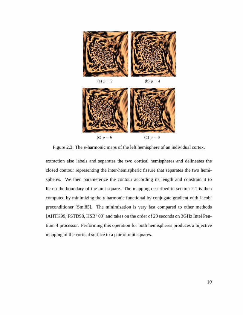


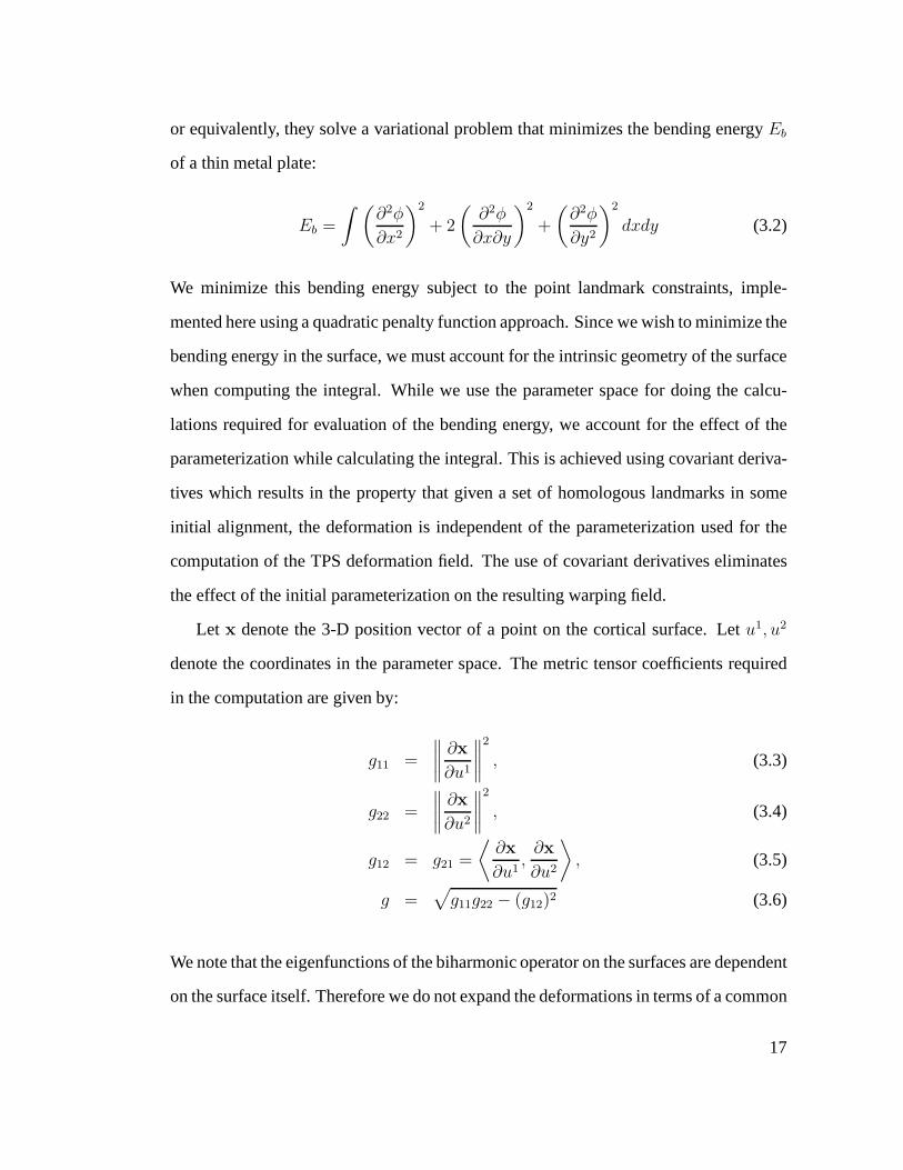


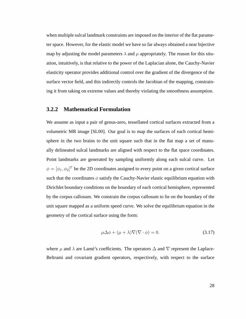


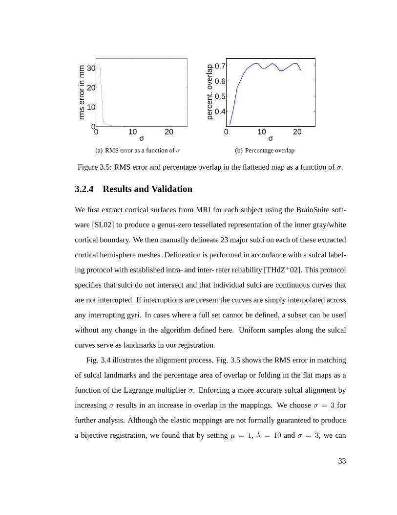


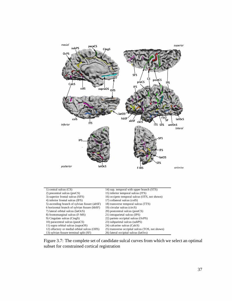


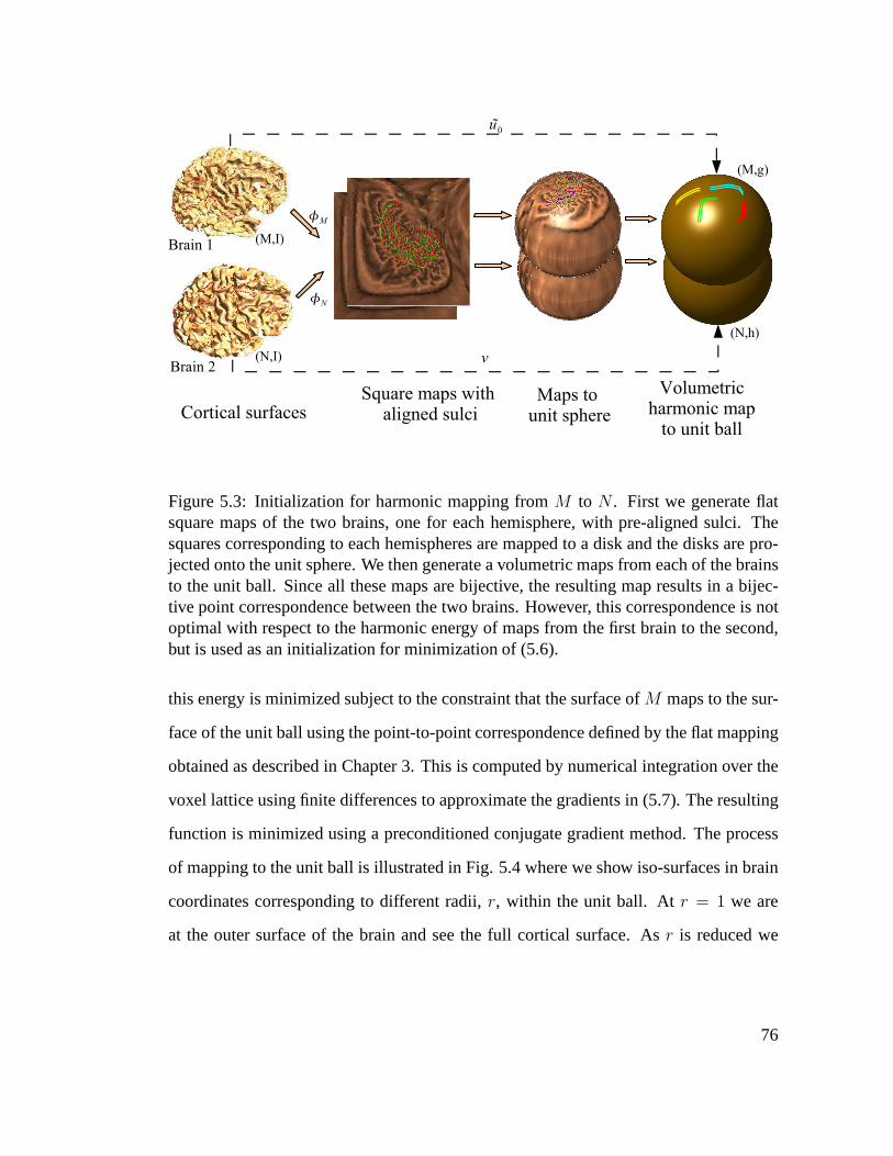


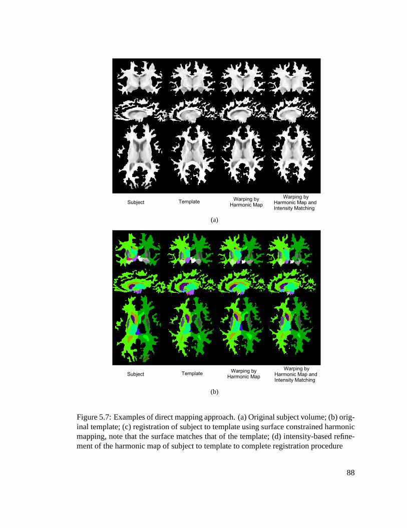


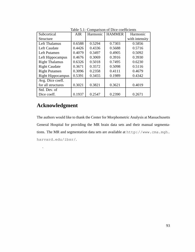


![Laboratory of Neuro Imaging, Department of Neurology, …users.loni.ucla.edu/~thompson/PDF/ALee-OHBM10_twinACE.pdf · MICCAI 2009: 498-506. [2] Jenkinson M., Smith, S.: A global optimization](https://static.documents.pub/doc/80x56/5ae748827f8b9a6d4f8dd755/laboratory-of-neuro-imaging-department-of-neurology-usersloniuclaeduthompsonpdfalee-ohbm10.jpg)
