22
Geometric Modeling 91.580.201 Curves (continued) Cubic Bezier and B-Spline Curves Farin Chapters 4-5, 6, 8 Mortenson Chapters 4, 5
| Date post: | 21-Dec-2015 |
| Category: |
Documents |
| View: | 237 times |
| Download: | 8 times |
Geometric Modeling91.580.201
Curves (continued)
Cubic Bezier and B-Spline CurvesFarin Chapters 4-5, 6, 8Mortenson Chapters 4, 5

4 Typical Types of Parametric Curves
• Interpolating– Curve passes through all control points.
• Hermite– Defined by its 2 endpoints and tangent vectors at endpoints.– Interpolates all its control points.– Not invariant under affine transformations.– Special case of Bezier and B-Spline.
• Bezier*– Interpolates first and last control points.– Invariant under affine transformations.– Curve is tangent to first and last segments of control polygon.– Easy to subdivide.– Curve segment lies within convex hull of control polygon.– Variation-diminishing.– Special case of B-spline.
• B-Spline*– Not guaranteed to interpolate control points.– Invariant under affine transformations.– Curve segment lies within convex hull of control polygon.– Variation-diminishing.– Greater local control than Bezier.
Control points influence curve shape.
source: Mortenson, source: Mortenson, AngelAngel
*focus of this lecture
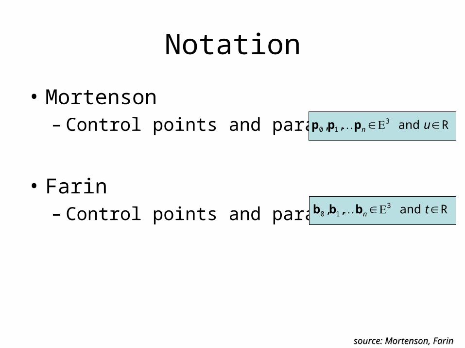
Notation
• Mortenson– Control points and parameter:
• Farin– Control points and parameter: R and ,, 3
10 tnbbb
R and ,, 310 unppp
source: Mortenson, Farinsource: Mortenson, Farin

Bezier CurvesFarin Chapter 4
The de Casteljau Algorithm

Parabola Construction
• Change of notation from Chapter 3 (previously):
• Now:
• Add:
• By substitution:
source: Farinsource: Farin
10)1(],0[ bbb ttt 21)1(],1[ bbb ttt
1010 )1()( bbb ttt
2111 )1()( bbb ttt
)()()1()( 11
10
20 ttttt bbb
22
1022
0 )1(2)1()( bbbb ttttt

The de Casteljau Algorithm
• Given:
• set:
• Example: cubic
rni
nr
,0
,1
source: Farinsource: Farin
)()()1()( 11
1 ttttt ri
ri
ri
bbbii t bb )(0
R and ,, 310 tnbbb
30
21
123
20
112
101
0
bbbb
bbb
bb
b
curve point
Conceptually elegant, but not necessarily the fastest algorithm…
source: Farinsource: Farin
21b

Some Bezier Curve Properties
• Affine invariance: Linear interpolation is affinely invariant.• Invariance under affine parameter transformations (beyond
[0,1] to [a,b]):
• Convex hull: Curve stays within convex hull of control polygon.– Each intermediate point is a convex barycentric combination of
previously generated points.– Planar control polygon generates planar curve.– Helpful for intersection tests.
• Endpoint interpolation: Curve passes through b0 and bn.– Verify using scheme for t =0 and t =1.
)()()( 11
1 uab
auu
ab
ubu r
iri
ri
bbb
source: Farinsource: Farin

Bezier CurvesFarin Chapter 5-6
& Mortenson Chapter 4The Bernstein Form of a Bezier Curve
Bezier
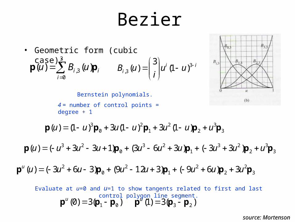
• Geometric form (cubic case):
3
03, )()(
iii uBu pp
source: Mortensonsource: Mortenson
iii uu
iuB
3
3, )1(3
)(
Evaluate at u=0 and u=1 to show tangents related to first and last control polygon line segment.
33
22
12
03 )1(3)1(3)1()( ppppp uuuuuuu
33
223
123
023 )33()363()133()( ppppp uuuuuuuuuu
32
22
12
02 3)69()3129()363()( ppppp uuuuuuuuu
Bernstein polynomials.
4 = number of control points = degree + 1
)(3)0( 01 ppp u )(3)1( 23 ppp u

Bezier
• Geometric form (general case):
n
iini uBu
0, )()( pp
source: Mortensonsource: Mortenson
inini uu
i
nuB
)1()(,
Bernstein polynomials.
n+1 = number of control points = degree + 1
Rational form is invariant under perspective transformation:where hi are projective space coordinates (weights)
n
inii
n
iinii
uBh
uBhu
0,
0,
)(
)()(
pp
See Chapter 13 of Farin for rational Bezier material.

More Bezier Curve Properties
• Symmetry: Bernstein polynomials are symmetric with respect to u and 1- u.
• Convex Hull (again):
source: Farin, Mortensonsource: Farin, Mortenson
Convex combination, so Bezier curve points all lie within convex hull of control polygon.
n
ini uB
0, 1)(
Bezier curve with 4 control points
inini uu
i
nuB
)1()(,
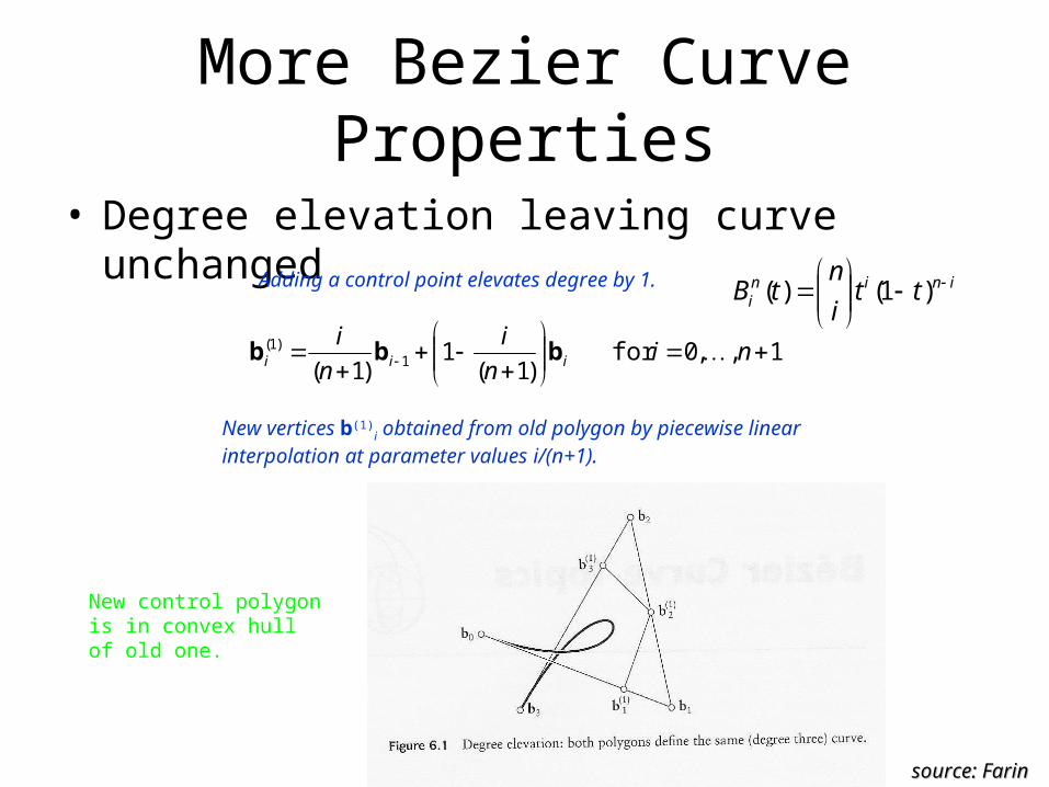
More Bezier Curve Properties
• Degree elevation leaving curve unchanged
inini tt
i
ntB
)1()(
source: Farinsource: Farin
Adding a control point elevates degree by 1.
1,,0for )1(
1)1( 1
)1(
nin
i
n
iiii bbb
New vertices b(1)i obtained from old polygon by piecewise linear
interpolation at parameter values i/(n+1).
New control polygon is in convex hull of old one.
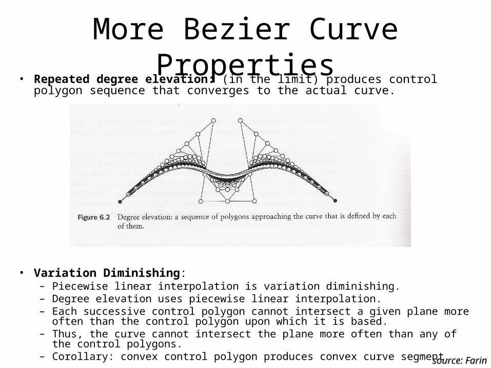
More Bezier Curve Properties• Repeated degree elevation: (in the limit) produces control polygon
sequence that converges to the actual curve.
• Variation Diminishing:– Piecewise linear interpolation is variation diminishing.– Degree elevation uses piecewise linear interpolation.– Each successive control polygon cannot intersect a given plane more often
than the control polygon upon which it is based.– Thus, the curve cannot intersect the plane more often than any of the control
polygons.– Corollary: convex control polygon produces convex curve segment.
source: Farinsource: Farin

Composite Bezier Curves
Evaluate at u=0 and u=1 to show tangents related to first and last control polygon line segment.
)(3)0( 01 ppp u )(3)1( 23 ppp u
Joining adjacent curve segments is an alternative to degree elevation.
source: Mortensonsource: Mortenson
Collinearity of cubic Bezier control points produces G1 continuity at join
point:
For G2 continuity at join point, 5 vertices must be coplanar.
B-Spline CurvesMortenson Chapter 5
& Farin Chapter 8

B-Spline
n
iiKi uNu
0, )()( pp
otherwise 0)(
if 1)(
1,
11,
uN
tutuN
i
iii
• Geometric form (non-uniform, non-rational case), where K controls degree (K -1) of basis functions:
• Cubic B-splines can provide C2 continuity at curve segment join points.
Convex combination, so B-spline curve points all lie within convex hull of control polygon.
n
iKi uN
0, 1)(
Rational form (NURBS) is invariant under perspective transformation, where hi are projective space coordinates (weights).
n
iKii
n
iiKii
uNh
uNhu
0,
0,
)(
)()(
pp
source: Mortensonsource: Mortenson
ti are n+1+K knot values that relate u to the control points.
Uniform case: space knots at equal intervals of u.
Repeated knots move curve closer to control points.
N
N
N N
N
N N
N N
See Chapter 13 of Farin for rational B-spline material.
1
1,1
1
1,,
)()()()()(
iki
kiki
iki
kiiki tt
uNut
tt
uNtuuN
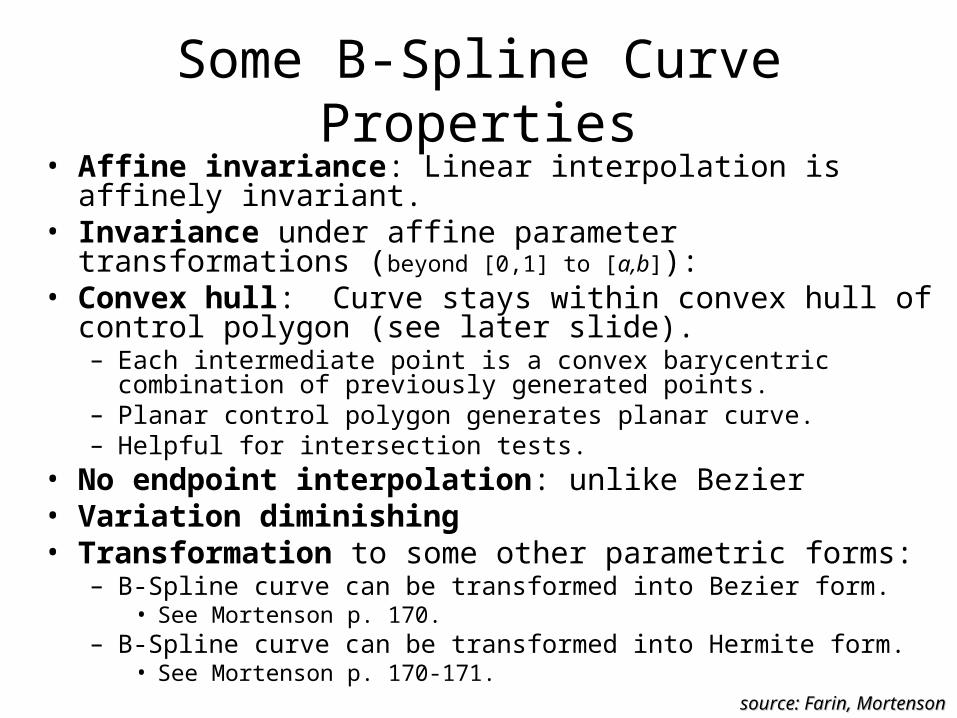
Some B-Spline Curve Properties• Affine invariance: Linear interpolation is affinely invariant.• Invariance under affine parameter transformations (beyond
[0,1] to [a,b]):• Convex hull: Curve stays within convex hull of control
polygon (see later slide).– Each intermediate point is a convex barycentric combination of
previously generated points.– Planar control polygon generates planar curve.– Helpful for intersection tests.
• No endpoint interpolation: unlike Bezier• Variation diminishing• Transformation to some other parametric forms:
– B-Spline curve can be transformed into Bezier form.• See Mortenson p. 170.
– B-Spline curve can be transformed into Hermite form.• See Mortenson p. 170-171.
source: Farin, Mortensonsource: Farin, Mortenson
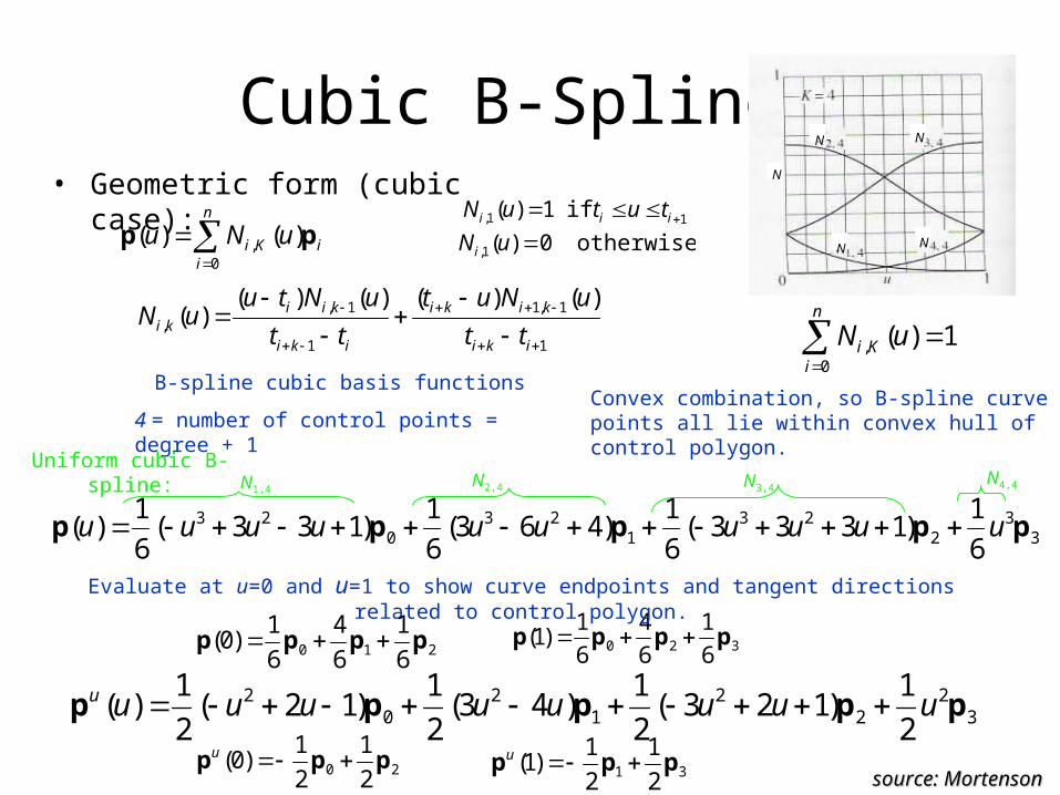
Cubic B-Spline • Geometric form (cubic case):
320 6
1
6
4
6
1)1( pppp
source: Mortensonsource: Mortenson
Evaluate at u=0 and u=1 to show curve endpoints and tangent directions related to control polygon.
32
22
12
02
2
1)123(
2
1)43(
2
1)12(
2
1)( ppppp uuuuuuuuu
B-spline cubic basis functions
4 = number of control points = degree + 1
20 2
1
2
1)0( ppp u
n
iiKi uNu
0, )()( pp
N
N N
N N otherwise 0)(
if 1)(
1,
11,
uN
tutuN
i
iii
1
1,1
1
1,,
)()()()()(
iki
kiki
iki
kiiki tt
uNut
tt
uNtuuN
Convex combination, so B-spline curve points all lie within convex hull of control polygon.
n
iKi uN
0, 1)(
33
223
123
023
6
1)1333(
6
1)463(
6
1)133(
6
1)( ppppp uuuuuuuuuu
Uniform cubic B-spline:N1,4
N2,4 N3,4N4,4
210 6
1
6
4
6
1)0( pppp
31 2
1
2
1)1( ppp u

More B-Spline Curve Properties
• Symmetry: Basis functions possess parametric symmetry:
source: Farin, Mortensonsource: Farin, Mortenson
Example: Uniform cubic B-spline:
33
223
123
023
6
1)1333(
6
1)463(
6
1)133(
6
1)( ppppp uuuuuuuuuu
N1,4N2,4 N3,4 N4,4
)1()( ,1, uNuN KiKKi

Shape Characterization of Uniform Cubic B-Spline Curve Segment
• Shape depends on control polygon• 3 (non-collinear) control points determine
triangle• Type of curve segment and its monotonicity
depends on location of 4th point p3 relative to triangle p0, p1, p2:
– SP: spiral control polygon induces convex, monotone curve segment.
– U: U-shaped convex control polygon induces convex, monotone curve segment.
– V:V-shaped convex control polygon induces 1 inflection point at curve segment endpoint. Curve segment is convex, monotone.
– N: N-shaped control polygon induces1 inflection point with convex, monotone pieces on both sides of inflection point.
– SI: self-intersecting control polygon induces 1 or 2 monotone curve subsegments.
– D: self-intersecting control polygon may induce loop, cusp or 2 inflection points.
– In all cases, curve segment can be partitioned into at most 2 monotone pieces.
p0
p1
p2
SPSP
SP
SPSP
SI
UV
V
N
N
N
SP
D
source: Daniels, et al. building on Wang et al.source: Daniels, et al. building on Wang et al.

The deBoor Algorithm
• Given: knots & control points
& parameter u, generalize de Casteljau algorithm.
• Example: quadratic case with 4 knots and 3 control points
source: Farinsource: Farin],[],[],[
],[],[
],[
232
121
10
uuuuuu
uuuu
uu
bbb
bb
b
curve point
Conceptually elegant, but not necessarily the fastest algorithm…
source: Farinsource: Farin
32110 ],[],,[ uuuu bb
,, 10 uu
],[],[],[ 212
11
12
2 uuuu
uuuu
uu
uuuu bbb
],[],[ 2102
010
02
2
12
2 uuuu
uuuu
uu
uu
uu
uubb
],[],[ 3213
121
13
3
12
1 uuuu
uuuu
uu
uu
uu
uubb
knot sequence u0, u1, u2, u3 = 0, 1, 3, 4 and u = 2.0
Geometric Modeling91.580.201
OpenGL Demoto accompany HW#2


