Geometric stability of topological lattice phases - TCM Group · Geometric stability of topological...

Geometric stability of topological lattice phases

Advanced(Numerical(Algorithms(for(Strongly(Correlated(Quantum(Systems,(Universität(Würzburg,(February(2015

arxiv:1408.0843

Thomas Jackson1, Gunnar Möller2, Rahul Roy1

1 2 2

Gunnar Möller Würzburg, February 2015

Overview

• Background: Topology and interactions in tight-binding models

• The role of band geometry in the Single Mode Approximation to quantum Hall liquids / fractional Chern insulators

• Role of band geometry for incompressible Hall liquids

screening of three target models


Quantum Hall Effect in Periodic Potentials

• quantized Hall response in filled bands:

E

n�

12

-1-2

• the Hofstadter spectrum provides bands of all Chern numbers

• filled bands in this spectrum yield a quantized Hall response

figure: Avron et al. (2003)

• Chern-number for periodic systems

Thouless, Kohmoto, Nightingale, de Nijs 1982

�xy

=e2

h

X

filled bands

Cn

H = �JX

h↵,�i

hb̂†↵b̂�e

iA↵� + h.c.i+

1

2UX

↵

n̂↵(n̂↵ � 1)� µX

↵

n̂↵

��

��

�

X

⇤A↵� = 2⇡n�

• Hofstadter model (solved 1976): tight-binding model for electrons in bands with finite Chern number

C = 12⇡

RBZ d2kB(k)


Fractional Quantum Hall Effect in Periodic Potentials

• quantized Hall response in partially filled bands?

• THEORY: Kol & Read (1993)

• Confirmations for such states?

H = �JX

h↵,�i

hb̂†↵b̂�e

iA↵� + h.c.i+

1

2UX

↵

n̂↵(n̂↵ � 1)� µX

↵

n̂↵+X

Vij n̂in̂j


Fractional Quantum Hall on lattices: Numerical Evidence

• interest in cold atom community 2000’s:

• realisations of tight-binding models with complex hopping from light-matter coupling:

B

H = �JX

h↵,�i

hb̂†↵b̂�e

iA↵� + h.c.i+

1

2UX

↵

n̂↵(n̂↵ � 1)� µX

↵

n̂↵

• bosons with onsite U: many-body gap in the half-filled “synthetic Landau-level” persists to large flux density


Fractional Quantum Hall on lattices with higher Chern-# bands

• bands of the Hofstadter model go beyond the continuum limit and support new classes of quantum Hall states

nmany-body gap predicted by CF theory �

n�

n = 1/7: O = |h CF|GSi|2 ' 0.56

n = 1/9: O = |h CF|GSi|2 ' 0.46

(N=5 particles)

numerical verification !for what we would now call FCI states with ν=1!• C=2 band!• hardcore bosonsE

kx

ky

C = �2GM & NR Cooper, PRL 2009

theory:!bosonic Hall states!on the lattice


Φ>0Φ<0

Chern bands in more general tight binding models

• 2011: FQHE could naturally in models with spin-orbit coupling + interactions

Numerical confirmation: D. Sheng; C. Chamon; N. Regnault & A. Bernevig, …

T. Neupert et al. K. Sun et al. E. Tang et al.

• Original proposal for IQHE without magnetic fields: Haldane (1988)

Chern numbers


Stability of Fractional Chern Insulators

• single-particle dispersion - want flat bands

• band geometry - ideally want even Berry curvature

• shape of interactions - clear hierarchy of two-body energies desirable “Pseudopotentials”

• Full story: all three aspects contribute

many groups

finite size matter a lot - success by iDMRG A. Grushin et al.

Regnault, Bernevig; Dobardzic, Milovanovic, …

Läuchli, Liu, Bergholtz, Moessner + other proposals

no systematic in-depth study of geometric measures This Talk!

How to decide which lattice models have stable fractional Chern Insulators?


Band Geometry: Berry Curvature and Chern Number

Basic notations:

|k, bi = 1pNc

X

R

eik·(R+db)|R, bi sublattice indexb = 1, . . . ,N

Fourier transform:

Single particle eigenstates:

1

2

|k,↵i =NX

b=1

u↵b (k)|k, bi = �̂↵†

k |vaciband index α

↵ = 1

↵ = 2

Hbc(k) =NX

↵=1

E↵(k)u↵⇤b (k)u↵

c (k)

Bloch Hamiltonian:

A↵(k) = �iNX

b=1

u↵⇤b rku

↵b

Berry connection:gauge dependent

Berry curvature: B↵(k) = r⇥A↵(k) gauge invariant

c1 =SBZ

2⇡hB↵iChern number: average <> over BZ, quantized to integer values


Which Berry Curvature?

Gauge invariance of the Bloch functions: one arbitrary U(1) phase for each k-point

|u↵ki ! ei�↵(k)|u↵

ki

Hbc(k) =NX

↵=1

E↵(k)u↵⇤b (k)u↵

c (k)

The above manifestly leaves H invariant:

u↵a (k) ! eu↵

b (k) = eirb·ku↵b (k)

However, sublattice dependent phases are not gauges:

eB↵

(k)�B↵

(k) =NX

b=1

rb,y

@

@kx

|u↵

b

(k)|2 � rb,x

@

@ky

|u↵

b

(k)|2

as this substitution yields a modified Berry curvature:

There is a unique choice such that the polarisation reduces to the correct semi-classical expression

see, e.g. Zak PRL (1989) R̂µ ! �i

@

@kµand canonical position operator


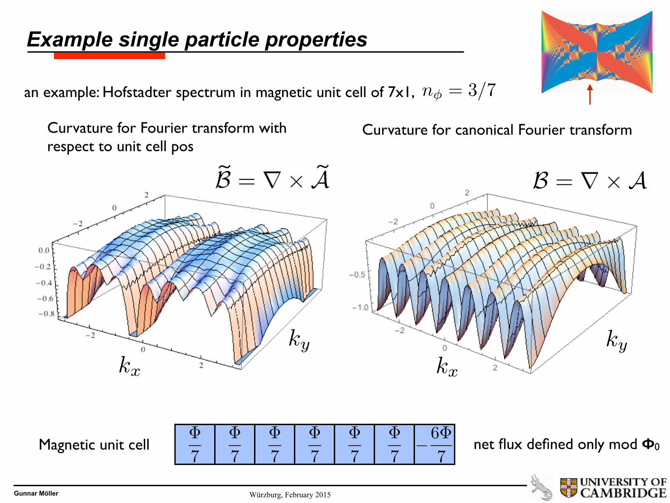
Example single particle properties

an example: Hofstadter spectrum in magnetic unit cell of 7x1,n = 1/7, n� = 3/7

kx

ky

B = r⇥A

Curvature for Fourier transform with respect to unit cell pos

Magnetic unit cell�

7

�

7

�

7

�

7

�

7

�

7�6�

7

kx

ky

B = r⇥A

Curvature for canonical Fourier transform

~ ~

net flux defined only mod !0


GMP Algebra: Generating low-lying excitations

[⇢LLL(q),⇢LLL(q0)] =

2i sin�12q ^ q0`2B

�exp

�12q · q0`2B

�⇢LLL(q+ q0

)

GMP algebra (w/LLL form factor):

S. M. GIRVIN, A. H. MacDONALD, AND P. M. PLATZMAN 33

wave vector, but exhibits a deep minimum at finite k.This magneto-roton minimum is caused by a peak in s(k)and is, in this sense, quite analogous to the rotonminimum in helium. ' We interpret the deepening of theminimum in going from v= —,

' to v= —,' to be a precursor

of the collapse of the gap which occurs at the critical den-sity v, for Wigner crystallization. From Fig. 3 we seethat the minimum gap is very small for v& —,. This isconsistent with a recent estimate of the critical density,v, =1/(6.5+0.5). Within mean-field theory, the Wignercrystal transition is weakly first order and hence occursslightly before the roton mode goes completely soft. Fur-ther evidence in favor of this interpretation of the rotonminimum is provided by the fact that the magnitude ofthe primitive reciprocal-lattice vector for the crystal liesclose to the position of the magneto-roton minimum, asindicated by the arrows in Fig. 3.These ideas suggest the physical picture that the liquid

is most susceptible to perturbations whose wavelengthmatches the crystal lattice vector. This will be illustratedin more detail in Sec. XI.Having provided a physical interpretation of the gap

dispersion and the magneto-roton minimum, we now ex-amine how accurate the SMA is. Figure 4 shows the ex-cellent agreement between the SMA prediction for the gapand exact numerical results for small (%=6,7}systems re-cently obtained by Haldane and Rezayi. Those authorshave found by direct computation that the single-modeapproximation is quite accurate, particularly near the ro-ton minimum, where the lowest excitation absorbs 98% ofthe oscillator strength. This means that the overlap be-tween our variational state and the exact lowest excitedeigenstate exceeds 0.98. We believe this agreement con-firms the validity of the SMA and the use of theLaughlin-state static structure factor.Near k =0 there is a small (-20%) discrepancy be-

tween b,sMA(0) and the numerical calculations. It is in-

v=1/3

L"S

Q. 10

0.05

VII. BACKFLOW CORRECTIONS

It is apparent from Fig. 4 that the SMA works extreme-ly well—better, in fact, than it does for helium. '9 Why isthis so'? Recall that, for the case of helium, theFeynman-Bijl formula overestimates the roton energy byabout a factor of 2. Feynman traces this problem to thefact that a roton wave packet made up from the trial wavefunctions violates the continuity equation

V (J)=0.To see how this happens, consider a wave packet

P(ri, . . . , rpg)= I d2k g(k)pkP(r„. . . , r~),(7.1)

(7.2)

where g(k) is some function (say a Gaussian) sharplypeaked at a wave vector k located in the roton minimum.It is important to note that this wave packet is quasista-tionary because the roton group velocity dhldk vanishesat the roton minimum. Evaluation of the current densitygives the result schematically illustrated in Fig. 5(a). Thecurrent has a fixed direction and is nonzero only in the re-gion localized around the wave packet. This violates thecontinuity equation (7.1} since the density is (approxi-mately) time independent for the quasistationary packet.The modified variational wave function of Feynman andCohen includes the backflow shown in Fig. 5(b}. Thisgives good agreement with the experimental roton energyand shows that the roton can be viewed as a smoke ring(closed vortex loop).A rather different result is obtained for the case of the

quantum Hall effect. The current density operator is

eA(rj }

teresting to speculate that the lack of dispersion near theroton minimum may combine with residual interactionsto produce a strong pairing of rotons of opposite momen-ta leading to a two-roton bound state of small totalmomentum. This is known to occur in helium. For thepresent case b, i~3(0) happens to be approximately twicethe minimum roton energy. Hence the two-roton boundstate which has zero oscillator strength could lie slightlybelow the one-phonon state which absorbs all of the oscil-lator strength. For v & —, the two-roton state will definite-ly be the lowest-energy state at k =0. It would be in-teresting to compare the numerical excitation spectrumwith a multiphonon continuum computed using thedispersion curves obtained from the SMA.

0.00O.Q 0.5 1.0 1.5 2.0 + p)+

eA(rj ) z5 (R—rj) (7.3)

FIG. 4. Comparison of SMA prediction of collective modeenergy for v= 3, 5, 7 with numerical results of Haldane andRezayi (Ref. 20) for v= —,. Circles are from a seven-particlespherical system. Horizontal error bars indicate the uncertaintyin converting angular momentum on the sphere to linearmomentum. Triangles are from a six-particle system with ahexagonal unit cell. Arrows have same meaning as in Fig. 3.

&+ IJ(R)

I+)=—-vx(e I M(R) I

+)where

M(R) =p(R)R,

(7.4)

(7.5)

Taking P and P to be any two members of the Hilbertspace of analytic functions described in Sec. IV, it isstraightforward to show that

Girvin, MacDonald and Platzman, PRB 33, 2481 (1986).

| SMAk i = ⇢̂k| 0i

• single mode approximation captures low-lying neutral excitations in quantum Hall systems:

Repellin, Neupert, Papić, Regnault, Phys. Rev. B 90 (2014)SMA carries over to Chern bands:

⇢̂k =X

q

�̂†k+q�̂qfor sp density operators


Chern bands: generalised GMP algebra

e⇢q ⌘ P↵eiq·brP↵ =

X

k

NX

b=1

u↵⇤b (k+ q/2)u↵

b (k� q/2)�↵†k+q/2�

↵k�q/2

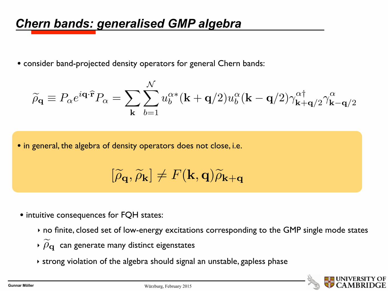
• consider band-projected density operators for general Chern bands:

• in general, the algebra of density operators does not close, i.e.

[e⇢q, e⇢k] 6= F (k,q)e⇢k+q

• intuitive consequences for FQH states:

e⇢q ⌘ P↵eiq·brP↵ =

X

k

NX

b=1

u↵⇤b (k+ q/2)u↵

b (k� q/2)�↵†k+q/2�

↵k�q/2can generate many distinct eigenstates

‣ no finite, closed set of low-energy excitations corresponding to the GMP single mode states

‣

‣ strong violation of the algebra should signal an unstable, gapless phase


Conditions for closure of the generalised GMP algebra I

�c ⌘r

A2BZ

4⇡2hB2i � c21

• conditions for closure can be derived in long-wavelength expansion

O(k2) :

O(k3) :

ds2 = h� |� i � h� | ih |� i

Pullback of Hilbert space metric constant over BZ

gµ⌫ + i2

Fµ⌫

=X

↵2occ

tr�

@@kµ

P↵

�(1� P↵)

�@

@k⌫P↵

�

�g ⌘s

1

2

X

µ,⌫

hgµ⌫g⌫µi � hgµ⌫ihg⌫µi

flatness of Berry curvature

deviaEons

i)

ii)


Conditions for closure of the generalised GMP algebra II

iii)((closure(at(all(orders(if

D(k) ⌘ det g↵(k)� B↵(k)2

4= 0

• if i), ii) and iii) are met, one obtains a generalised GMP algebra:

[e⇢q, e⇢k] = 2ieP

µ,⌫ g↵µ⌫qµk⌫ sin

✓B↵

2q ^ k

◆e⇢q+k

• under stronger variant of condition iii) the algebra reduces exactly to the GMP algebra, namely if

T (k) ⌘ tr g↵(k)� |B↵(k)| = 0;

• Current study: test how violations of the closure constraints correlate with gap

R. Roy, arxiv:1208.2055 (PRB 2014); Parameswaran, Roy, Sondhi C. R. Physique (2013)


Target models to examine

• Hamiltonian: bosonic states with on-site interactions — defined independent of specific lattice

2Gbody(contact 3Gbody(contact

⌫ =1

2Laughlin ⌫ = 1MooreGRead

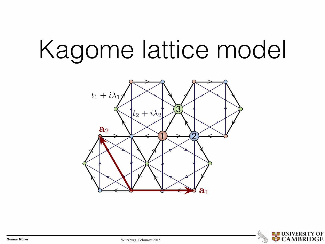
• lattice geometries to consider:

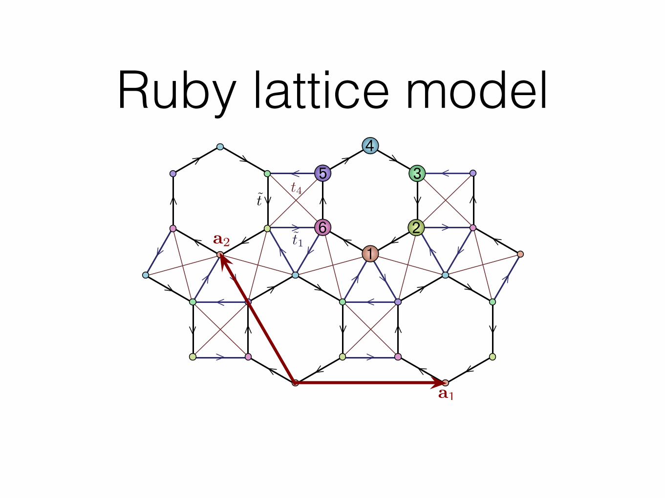
Haldane(model Kagomé(model Ruby(laOce(model

➁➀

t2ei�

t1a2

a1

N = 2

a2

a1

➁➀

➂t2 + i�2

t1 + i�1

N = 3

➀➁

➂➃

➄

➅a2

a1

t̃1

t4t̃

N = 6


➁➀

t2ei�

t1a2

a1

Haldane modelt3

‡

‡

‡

‡

‡

‡‡‡‡‡‡

‡‡‡‡‡‡‡‡‡‡‡‡‡‡‡‡‡‡‡‡‡‡‡‡‡‡‡‡‡ ‡

‡ ‡‡ ‡ ‡‡

0.8

1.0

1.2

1.4

1.6

1.8

2.0

sc

Ï

Ï

ÏÏÏÏÏÏÏÏÏÏÏÏÏÏÏÏ

ÏÏÏÏÏÏÏÏÏÏÏÏÏÏÏÏÏÏÏÏÏÏÏ

Ï ÏÏ Ï

Ï Ï Ï

Ï

Ú

Ú

ÚÚÚÚÚÚÚÚÚÚÚÚÚÚÚÚ

ÚÚÚÚÚÚÚÚÚÚÚÚÚÚÚÚÚÚÚÚÚ ÚÚ Ú

Ú Ú ÚÚ Ú Ú Ú

0

5

10

15

20

sg,XT\

‡ scÏ sgÚ XT\

Ê

Ê

Ê

Ê

Ê

ÊÊÊÊÊÊÊÊÊÊÊÊÊÊÊÊÊÊÊÊ

ÊÊÊÊÊÊÊÊ Ê Ê Ê Ê Ê Ê Ê Ê Ê Ê

Ê

0.0 0.5 1.0 1.5

0.06

0.08

0.10

0.12

0.14

0.16

0.18

f

DHbos

onsL

Á

Á

ÁÁÁÁÁÁÁÁÁÁÁÁÁÁÁÁÁÁÁÁÁÁÁÁÁÁÁÁÁÁÁÁÁÁÁÁ Á Á

Á Á Á Á Á Á Á

Á 0.010

0.015

0.020

0.025

DHferm

ionsL

Ê n=1ê2 bosonsÁ n=1ê3 fermions

0.0 0.2 0.4 0.6 0.8 1.0 1.2 1.40

1

2

3

4

5

f

M

0.0 0.2 0.4 0.6 0.8 1.0 1.2 1.40.0

0.5

1.0

1.5

2.0

2.5

f

M

(a)

(b)

(c)

(d)

• Location of max gap for bosonic and fermionic Laughlin agrees with min RMS B • Band geometry “interpolates” between bosonic, fermionic statistics • For this model, quantum metric does not provide info beyond that supplied by

curvature.

Haldane Model with t3=0

Laughlin: Bosons

Laughlin: Fermions

Curvature

Gap

Jackson, GM, Roy, arxiv:1408.0843; cf. Dobardzic, Milovanovic and Regnault, PRB 2013)

�� -��

-��

-��

-��

-��

��

��

��

� �

��

�

�

�

�

�

�

�� -��

-��

-��

-��

-��

��

��

��

� �

��

�

�

�

�

�

�

• position of maximum gap appears to be compromise between minimising curvature fluctuations and metric trace inequality (also seen in fermionic Laughlin)

�� -��

-��

-��

-��

-��

��

��

��

� �

��

��

��

��

��

�

�� -��

-��

-��

-��

-��

��

��

��

� �

�� -��

��

��

��

��

��

��

��

�

Haldane Model: Effects of quantum metric for M=0, t3>0


a2

a1

➁➀

➂t2 + i�2

t1 + i�1

Kagome lattice model

sc0.0 0.5 1.0 1.5 2.0 2.5 3.0 3.5

0.06

0.08

0.10

0.12

0.14

0.16

0.18

D

HaL0.225 0.250 0.275 0.300 0.325 0.350 0.375 0.400

0.150

0.155

0.160

0.165

0.170

0.175

0.180

HbL

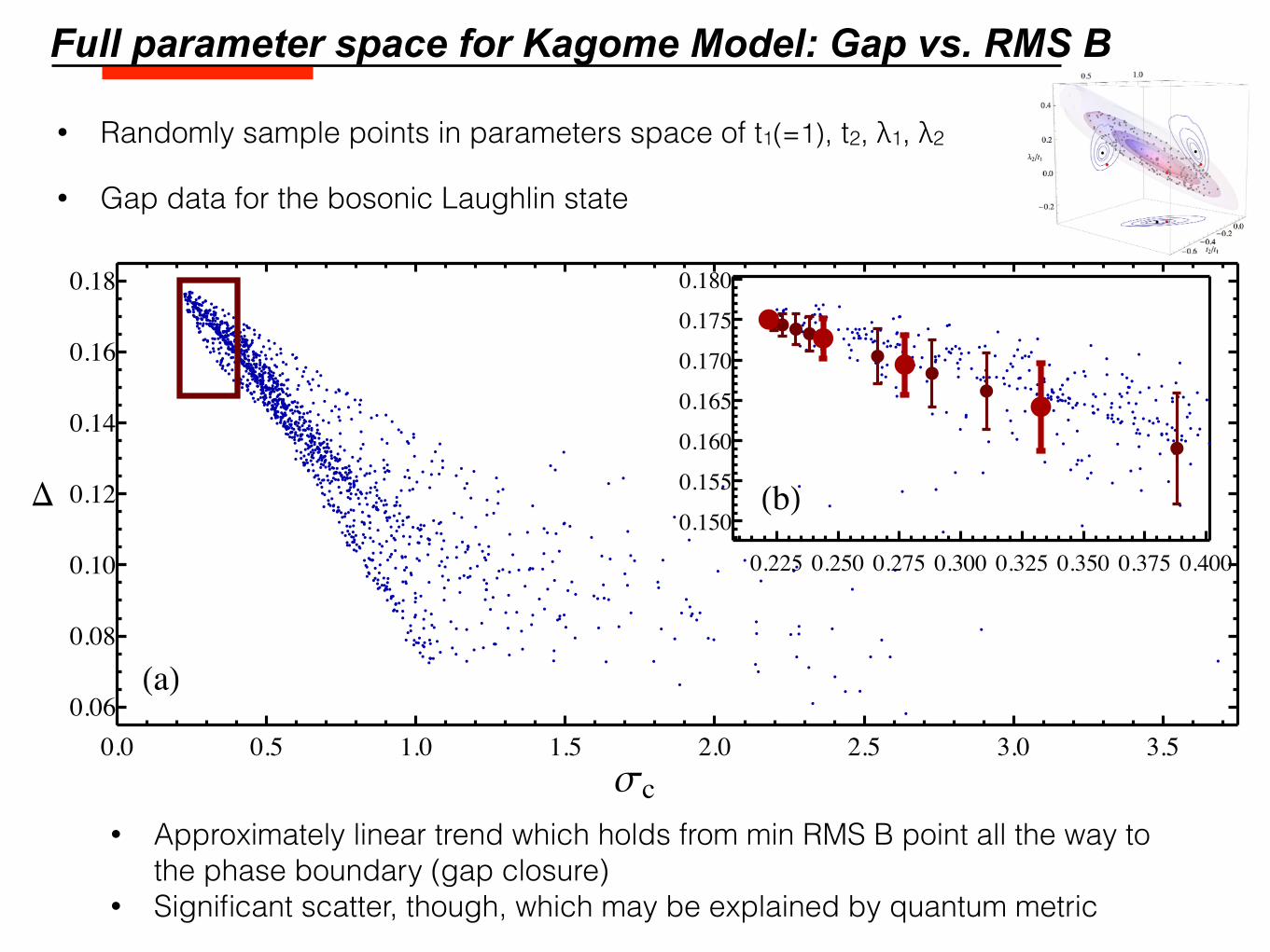
• Approximately linear trend which holds from min RMS B point all the way to the phase boundary (gap closure)

• Significant scatter, though, which may be explained by quantum metric

Full parameter space for Kagome Model: Gap vs. RMS B

• Randomly sample points in parameters space of t1(=1), t2, λ1, λ2

• Gap data for the bosonic Laughlin state


��

��

��

��

��

��

�

�<� ��

(�)

��

�=��

(�)

��

�=��

(�)

��

�=��

(�)

��

�=��

(�)

�� -��

�� <�>

��

�

��<� ��

(�)

�� <�>

��=��

(�)

�� <�>

��=��

(�)

�� <�>

��=��

(�)

�� <�>

��=��

(�)

• Considering models at surfaces of fixed σc, the violation of the metric trace equality ⟨T⟩ is highly correlated with the many-body gap

Kagome Model: “Shells” of constant RMS Curvature

TS Jackson, G. Möller, R. Roy “Geometric stability of topological lattice phases”, arxiv:1408.0843

Ruby lattice model

➀➁

➂➃

➄

➅a2

a1

t̃1

t4t̃


sc0.0 0.5 1.0 1.5 2.0 2.5

0.04

0.06

0.08

0.10

D

HaL0.14 0.16 0.18 0.20 0.22 0.24 0.26

0.075

0.080

0.085

0.090

0.095

0.100

HbL

• Similar linear dependence of gap on RMS B as seen in Kagome model

Ruby Lattice Model: Gap vs RMS Curvature


• Even clearer results for influence of metric trace inequality ⟨T⟩

��

��

��

��

��

��

��

�

�<� ��

(�)

��

�=��

(�)

��

�=��

(�)

��

�=��

(�)

��

�=��

(�)

�� -��

�� <�>

��

��

��

��

��

�

�<� ��

(�)

�� <�>

�=��

(�)

�� <�>

�=��

(�)

�� <�>

�=��

(�)

�� <�>

�=��

(�)

Ruby Lattice Model: “Shells” of constant RMS Curvature

Models with many sub lattices can approximate Landau level physics more closely

• Parameters yielding max gap are always in lower-left corner • Demonstrates relevance of both band-geometric quantities

Model Comparison: Gaps vs. RMS B and trace inequality

Haldane(model Kagomé(model Ruby(laOce(model

Laughlin(state

Moo

reGRead(state

curvature

trace

trace

curvaturecurvature


Conclusions

• Band geometry provides useful information about stability of fractional Chern insulators

• Berry curvature O(k2) is the dominant effect (as previously known)!• Trace of the quantum metric O(k3) provides further information

• Statistically, band geometry is strongly correlated with many-body gap

• But: it is only one of three factors, so not the only important measure

useful for quick exploration of available parameter space

Related works: Adiabatic continuity T. Scaffidi & GM, Phys. Rev. Lett. 109, 246805 (2012)

FCI in the Hofstadter model GM & N. R. Cooper, Phys. Rev. Lett. 103, 105303 (2009)

TS Jackson, G. Möller, R. Roy “Geometric stability of topological lattice phases”, arxiv:1408.0843

Quantifying degree of correlation on shells of const. RMS B — Spearman ρ monotonicity test

��

�� -��

��

��

��

��

��

��

��

-�

��

��

�� -��

��

��

��

��

��

��

��

-�

��

• Nonparametric statistic which is sensitive to any monotonic relationship • Perfect correlation for ρ = ±1, no correlation at ρ = 0 • Find siginifcant, robust negative correlation between gap and metric

inequality on all isosurfaces of constant RMS B, demonstrating importance of trace inequality as a subleading influence on the gap

max DF min sc max DB BêB

b1

b2

b1

b2

b1

b2

BêB

0

1

2

3

4

5

BêB

-1.4

-1.2

-1.0

-0.8

-0.6

-0.4

-0.2

0.0

b1

b2

b1

b2

BêB

0.80

0.85

0.90

0.95

1.00

1.05

b1

b2

b1

b2

Plots of quantum metric across the BZ

Standard Haldane

Kagome

Ruby

0.0 0.5 1.0 1.5 2.0 2.5!0.02

0.00

0.02

0.04

0.06

0.08

0.10

Σc

#

Λ1

0.5

1.0

1.5

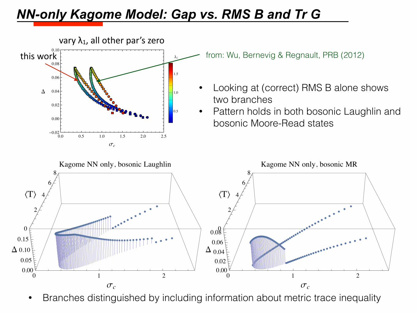
• Looking at (correct) RMS B alone shows two branches

• Pattern holds in both bosonic Laughlin and bosonic Moore-Read states

��

� � ��

�

�

�

��

��

��

��

�

��

� � ��

�

�

�

��

��

��

�

vary%λ1,%all%other%par’s%zero

NN-only Kagome Model: Gap vs. RMS B and Tr G

from: Wu, Bernevig & Regnault, PRB (2012)this%work

• Branches distinguished by including information about metric trace inequality

Geometry & gap for new parametrization of Haldane-t3

�� -��

-��

-��

-��

-��

��

��

��

� �

��

�

�

�

�

�

�

�� -��

-��

-��

-��

-��

��

��

��

� �

��

�

�

�

�

�

�

�� /�

b1

b2

b1

b2

b1

b2

• Now have large range of parameters with uniform curvature • Minimum trace inequality in distinct location from min RMS B

Date post:	20-Jan-2019
Category:	Documents
Upload:	trinhkiet
View:	217 times
Download:	0 times

Geometric stability of topological lattice phases - TCM Group · Geometric stability of topological...

Documents