Geophysical Journal InternationalGeophys. J. Int. (2013) 194, 1665–1681 doi: 10.1093/gji/ggt178Advance Access publication 2013 June 14

GJI

Sei

smol

ogy

Multiparameter full waveform inversion of multicomponentocean-bottom-cable data from the Valhall field. Part 2: imagingcompressive-wave and shear-wave velocities

Vincent Prieux,1 Romain Brossier,2 Stephane Operto1 and Jean Virieux2

1Geoazur, Universite Nice-Sophia Antipolis, CNRS, IRD, Observatoire de la Cote d’Azur, Valbonne, CGG Massy, France. E-mail: vincent.prieux@cgg.com2ISTerre, Universite Joseph Fourier Grenoble 1, CNRS, Grenoble, France

Accepted 2013 May 1. Received 2013 April 23; in original form 2012 July 30

S U M M A R YMultiparameter elastic full waveform inversion (FWI) is a promising technology that allowsinferences to be made on rock and fluid properties, which thus narrows the gap betweenseismic imaging and reservoir characterization. Here, we assess the feasibility of 2-D verticaltransverse isotropic visco-elastic FWI of wide-aperture multicomponent ocean-bottom-cabledata from the Valhall oil field. A key issue is to design a suitable hierarchical data-drivenand model-driven FWI workflow, the aim of which is to reduce the nonlinearity of the FWI.This nonlinearity partly arises because the shear (S) wavespeed can have a limited influenceon seismic data in marine environments. In a preliminary stage, visco-acoustic FWI of thehydrophone component is performed to build a compressional (P)-wave velocity model, adensity model and a quality-factor model, which provide the necessary background modelsfor the subsequent elastic inversion. During the elastic FWI, the P and S wavespeeds are jointlyupdated in two steps. First, the hydrophone data are inverted to mainly update the long-to-intermediate wavelengths of the S wavespeeds from the amplitude-versus-offset variations ofthe P–P reflections. This S-wave velocity model is used as an improved starting model forthe subsequent inversion of the better-resolving data recorded by the geophones. During thesetwo steps, the P-wave velocity model is marginally updated, which supports the relevance ofthe visco-acoustic FWI results. Through seismic modelling, we show that the resulting visco-elastic model allows several P-to-S converted phases recorded on the horizontal-geophonecomponent to be matched. Several elastic quantities, such as the Poisson ratio, and the ratioand product between the P and S wavespeeds, are inferred from the P-wave and S-wave velocitymodels. These attributes provide hints for the interpretation of an accumulation of gas belowlithological barriers.

Key words: Inverse theory; Elasticity and anelasticity; Controlled source seismology; Com-putational seismology; Wave propagation.

I N T RO D U C T I O N

Subsurface lithology and reservoir characterization require quanti-tative estimations of the physical rock properties. The joint knowl-edge of the compressional (P)-wave and shear (S)-wave velocities isof primary interest for better fluid characterization (Gregory 1976)as a potential indicator of hydrocarbon reservoirs (Tatham & Stoffa1976), or to estimate porosity and grain size through empirical re-lationships between porosity and the P or S wavespeeds (Domenico1984). Shear wave velocity models can also be used for the pro-cessing of multicomponent seismic data, as for wavefield decom-position or static corrections (Muyzert 2000). Full waveform inver-sion (FWI, Virieux & Operto 2009) is today mostly used to derive

P-wave velocity background models in acoustic approximations forreverse-time migration (Sirgue et al. 2010). However, multiparame-ter FWI based on the visco-elastic wave equation provides the neces-sary framework to evolve beyond the velocity model building task,and to derive more realistic multiparameter subsurface models, aspromoted by Tarantola (1986), Shi et al. (2007), Sears et al. (2008),Brossier (2011) and others. Applications of elastic FWI to real dataremain challenging because of the computational cost of the elasticmodelling, which is between one and two orders of magnitude moreexpensive in two dimensions than its acoustic counterpart (Brossier2011), and the strong nonlinearity of the elastic multiparameterinversion. In marine environments, the nonlinearity of the elasticFWI of streamer or multicomponent ocean-bottom seismic data can

C© The Authors 2013. Published by Oxford University Press on behalf of The Royal Astronomical Society. 1665

1666 V. Prieux et al.

result from the limited influence of the S wavespeed on the data,as a P-to-S conversion at the seabed or at deeper interfaces mustoccur to record S waves (Sears et al. 2008; Brossier et al. 2010b).On land, it is still an open question whether high-amplitude surfacewaves carry useful and manageable information for FWI (Brossieret al. 2009a; Baumstein et al. 2011).

Pioneering applications of elastic FWI to marine and landdata sets have been presented previously, where the P and/or Swavespeeds (VP, VS), the elastic impedances (IP, IS) and the Pois-son ratio (ν) have been reconstructed from short-spread reflectiondata (with less than 5 km offset) (Crase et al. 1990, 1992; Sun &McMechan 1992; Igel et al. 1996; Djikpesse & Tarantola 1999a).More recently, the application of FWI to long-spread streamer datawas also presented by Freudenreich et al. (2001) and Shipp & Singh(2002), although only the P wavespeed was updated during the in-version in this latter study.

The recording of multicomponent wide-aperture data is a keyfor the success of multiparameter elastic FWI, in addition to therecording of low frequencies (Manukyan et al. 2012). It is wellacknowledged that short-spread streamer acquisitions do not al-low for the reconstruction of the intermediate wavelengths of thesubsurface, because of the insufficient wide-aperture illumination(i.e. large scattering angles) (Jannane et al. 1989; Neves & Singh1996). This justifies the scale separation that underlies the two maintasks of the workflow of conventional seismic reflection process-ing: velocity macro-model building by traveltime tomography ormigration-based velocity analysis, and reflectivity imaging by mi-gration. Wide-aperture geometries provide a suitable framework tobuild the long and intermediate wavelengths of the subsurface fromlong-offset data, and hence they continuously sample the wavenum-ber spectrum of this subsurface (Sirgue & Pratt 2004). Secondly,wide-aperture multicomponent recordings are necessary to provideall of the scattering modes (the P–P, P–S, S–P and S–S diffractions)over a sufficiently broad range of scattering angles, which shouldhelp in the reconstruction of the S-wave velocity model. This iseven more critical in marine environments, where the waves shouldundergo at least one P-to-S conversion to allow for S-wave record-ing by sea-bottom acquisitions. Furthermore, the amount of P-to-Sconversion can be quite limited in the case of a soft seabed environ-ment, and in particular with the recording times used in classicalsurveys. Another key issue related to S-wave velocity imaging isthe building of a sufficiently accurate starting model for FWI. Thesmaller wavelengths of the shear wavefields make the reconstructionof the S-wave velocity subject to cycle skipping artefacts, and thismight prevent the continuous sampling of the wavenumber spec-trum of the S-wave velocity model. A second difficulty is relatedto the picking of reliable P-to-S converted phases for reflection-traveltime tomography: the construction of an initial S-wave modelis therefore more difficult than the construction of an initial P-wavemodel.

Mitigating nonlinearities is challenging, especially when elasticseismic data are considered. The strategy for feeding the optimiza-tion procedure by the seismic data is of primary importance, andthis can lead to the success or failure of the inversion procedure(Brossier et al. 2009b). The selection of the parameters is also ofimportance, and they might have different footprints in the recordeddata. Many hierarchical FWI strategies can be viewed to reduce thenonlinearity of the inversion when multicomponent data are invertedto reconstruct multiple classes of parameters (e.g. Tarantola 1986).A data-driven level of hierarchy can be designed by proceedingfrom the inversion of low frequencies to higher ones, such that inthe framework of multi-scale imaging, the large wavelengths of the

subsurface are reconstructed before the smaller ones (e.g. Bunkset al. 1995; Sirgue & Pratt 2004). Additional data precondition-ing can be viewed to inject progressively more resolution or morecomplex information into the inversion, by proceeding from earlyarrivals to later arrivals (Brossier et al. 2009b), or by proceedingfrom short offsets to longer offsets in the framework of the layer-stripping strategies (Shipp & Singh 2002; Wang & Rao 2009). In theframework of multicomponent data, the hierarchy with which thedata components are injected into the inversion is also a key feature,as the sensitivity of the data to one model parameter can dependon the data component (e.g. hydrophone versus geophone) (Searset al. 2008, 2010). When multiparameter inversion is performed,additional levels of hierarchy in the model space can also be con-sidered during FWI. First, the imaging of the parameters that havea dominant influence on the data can be chosen, before the imagingof the secondary parameters (Tarantola 1986). Secondly, the modelparameters that have influence on the wide-aperture components ofthe data can be reconstructed before those that have influence on theshort-aperture components of the data. According to the relationshipbetween the aperture (or the scattering) angles and the wavenum-ber spanned in the model (Miller et al. 1987; Pratt & Worthington1990; Jin et al. 1992; Sirgue & Pratt 2004), this strategy impliesthat the long wavelengths of the former category of parameters isreconstructed before the short wavelengths of the later category ofparameters, hence honouring the multi-scale approach of FWI. Afeasibility analysis of elastic FWI of multicomponent ocean-bottomseismic data was presented by Sears et al. (2008). They proposeda hierarchical approach, where the intermediate wavelengths of theS wavespeeds are first updated from the amplitude-versus-offset(AVO) variations of the P–P reflections on the hydrophone compo-nent. Although the influence of the shear-impedance contrasts onthe P–P reflection is one order of magnitude smaller than that ofthe P-wave impedance (Igel & Schoenberg 1995), the informationcarried by the P–P scattering mode to reconstruct the intermedi-ate wavelengths of the S-wave velocity model is quite importantin marine environments. Indeed, the elastic inversion of the wide-aperture P–P reflection wavefield can be seen as a tool to build areliable S-wave starting velocity model for the waveform inversionof the more resolving P-to-S converted phases recorded on the geo-phone components. In this study, we will reproduce this hierarchicalapproach that was presented in Sears et al. (2008).

We demonstrate an application of 2-D, multiparameter elasticFWI of multicomponent wide-aperture data recorded by ocean-bottom cables (OBCs) in the Valhall field. The reconstruction ofthe first P-wave velocity model, density model and attenuationmodel from the hydrophone component in the visco-acoustic ap-proximation was presented in a companion report that we refer toas ‘Paper I’ in the following (Prieux et al. 2013). In the first part,we review the main features of the elastic FWI method that weuse. Then, we review several aspects of multiparameter FWI ofmulticomponent data. In particular, the three key issues that are ad-dressed are the choice of the subsurface parametrization for elasticFWI, the hierarchy with which the different classes of parametersare updated, and the hierarchy with which the different data com-ponents are inverted. After a qualitative interpretation of the dataand the description of the set-up of the FWI, we present the FWIP-wave and S-wave velocity models, and we validate their relevanceagainst sonic logs, seismic modelling and source wavelet estima-tion. Finally, from the FWI velocity models, we build some elasticproperties, such as the Poisson ratio, and the product and ratio be-tween the P and S wavespeeds, that are amenable to geologicalinterpretations.

Multiparameter visco-elastic FWI on OBC data 1667

V I S C O - E L A S T I C F U L L WAV E F O R MI N V E R S I O N O F M U LT I C O M P O N E N TDATA

We seek to reconstruct the vertical P wavespeed and the S wavespeedby visco-elastic vertical transverse isotropic (VTI) FWI of the hy-drophone and geophone data. Large-scale models of the anisotropicparameters δ and ε are kept fixed, and were inferred by 3-Danisotropic reflection traveltime tomography (courtesy of BritishPetroleum). FWI is performed in the frequency domain by local opti-mization, where the gradient of the misfit function is computed withthe adjoint-state method (Plessix 2006; Chavent 2009). More specif-ically, a frequency-domain, velocity-stress, finite-element, discon-tinuous Galerkin method based on piecewise constant (P0), lin-ear (P1) and quadratic (P2) interpolation functions (Brossier et al.2010a; Brossier 2011) is used for the computing of the incident andadjoint wavefields. At the same time, a forward-modelling operatorbased on the second-order wave equation for particle velocities andthe P0 interpolation function is used to build the diffraction kernelof the FWI from self-adjoint operators (see Paper I and Brossier(2011)).

The misfit function C(m) is given by:

C(m) = 1

2

Nc∑j=1

�d†j Wd j �d j

+ 1

2

Np∑i=1

λi

(mi − mpriori

)†Wmi

(mi − mpriori

), (1)

where �d = (�d1, . . . , �dNc ) and Nc denote the multicomponent,data-residual vector and the number of data components involvedin the inversion, respectively. In this study, Nc is equal to 1 or 2,depending whether the hydrophone or the two geophone compo-nents are considered during the inversion. Each component j of thedata residual vector is weighted by the weighting matrix Wd j . Thismatrix can weight the data residuals according to the standard er-ror and/or according to the source–receiver offsets (Ravaut et al.2004; Operto et al. 2006). The multiparameter subsurface modelis denoted by m = (m1, ..., mNp ), where Np denotes the number ofparameter classes. In this study, the two classes of parameter arethe vertical P wavespeed and the S wavespeed, which are jointlyupdated here. A Tikhonov regularization is applied to each param-eter class i through a weighting operator Wmi , which forces thedifference between the model mi and the prior model mpriori

to besmooth. The scalars λi control the weight of the data-space mis-fit function 1

2

∑Ncj=1 �d†

j Wd�d j relative to the model-space misfitfunctions (mi − mpriori

)†Wmi (mi − mpriori). Of note, the scalar λi

can be adapted to each parameter class i, which helps to account forthe variable sensitivity of the data to each parameter class, as shownin Paper I.

The solution for the perturbation model, which minimizes themisfit function at iteration k, is given by:

�m(k) =

�(

W−1m J(k)t

Wd J(k)t + W−1m

(∂J(k)t

∂mT

) (�d(k)∗ ...�d(k)∗) + �

)−1

× �(

W−1m J(k)t

Wd�d(k)∗ + �(m(k) − mprior

)), (2)

where � is a block diagonal damping matrix that can be expressedas:

� =

⎛⎜⎜⎝λ1IM ... 0

... ... ...

0 ... λNp IM ,

⎞⎟⎟⎠ (3)

where IM is the identity matrix of dimension M, the number ofparameter unknowns per class of parameter. In eq. (2), � is thereal part of a complex number. The matrices Wd and Wm are Nc ×Nc and Np × Np block diagonal matrices, where each block isformed by the Wd j and Wmi matrices, respectively. The first termin eq. (2) is the inverse of the full Hessian, while the second termin eq. (2) is the gradient of the misfit function. In eq. (2), thematrix J is the sensitivity matrix, the coefficients of which are thevalues of the partial derivative of the wavefields with respect to themodel parameters at the receiver positions. These partial derivativewavefields are the solution of the wave equation:

B (ω, m(x))∂v (ω, x)

∂ml= −∂B (ω, m(x))

∂mlv (ω, x) , (4)

where B(ω, m(x)) is the forward-problem operator, and v is the in-cident particle velocity wavefield. The right-hand side of eq. (4) isthe secondary virtual source of the partial derivative wavefield, thespatial support and temporal support of which are centred on the po-sition of the diffractor ml (the index l runs over all of the parameters)and on the arrival time of the incident wavefield at the diffractor ml,respectively (Pratt et al. 1998). The scattering or diffraction patternof this virtual source is given by ∂B(ω, m(x))/∂ml, which givessome insight into the sensitivity of the data to the parameter ml as afunction of the scattering (or aperture) angle.

We use the quasi-Newton limited-memory Broyden-Flechter-Goldfarb-Shanno (L-BFGS) optimization algorithm for solvingeq. (2) (Nocedal 1980; Nocedal & Wright 1999). The L-BFGSalgorithm computes recursively an approximation of the product ofthe inverse of the Hessian with the gradient, from a few gradientsand a few solution vectors from the previous iterations. As an initialguess for this iterative search, we use a diagonal approximation ofthe approximate Hessian (the linear term) damped by the � matrix,

H0 =(

W−1m diag

{J(k)†Wd J(k)

}+ �

)−1. (5)

There are various expressions of eq. (2) (Greenhalgh et al. 2006)that can be selected for implementation convenience. Our imple-mentation allows the pre-conditioner of the L-BFGS algorithm(eq. 5) to be diagonal, and hence easy to invert, because matrix �

is diagonal, unlike Wm . The smoothing operators W−1mi

are Laplacefunctions that are given by:

W−1mi

(z, x, z′, x ′) = σ 2i (z, x) exp

(−|x − x ′|τx

)exp

(−|z − z′|τz

),

(6)

where quantities τ x and τ z denote the horizontal and vertical cor-relation lengths, defined as a fraction of the local wavelength. Thecoefficient σ i represents the standard error and can be scaled to thephysical unit or to the order of magnitude of the parameter class i. ALaplace function is used for W−1

mi, because its inverse in the expres-

sion of the misfit function can be computed analytically (Tarantola2005, p. 97–99).

1668 V. Prieux et al.

W H I C H PA R A M E T R I Z AT I O N F O RE L A S T I C F U L L WAV E F O R MI N V E R S I O N ?

The choice of the subsurface parametrization should be driven byat least three criteria: (i) The sensitivity of the data to the parame-ter with respect to the scattering angle (which is referred to as thediffraction pattern of the parameter) should be as broad as possible,to guarantee a broadband reconstruction of the selected parameter.This sensitivity is given by the directivity of the virtual source ineq. (4). (ii) On the other hand, the trade-off between the parameterclasses should be reduced as much as possible, which requires thatthe diffraction pattern of each parameter class does not significantlyoverlap as a function of the scattering angle. A suitable trade-offbetween these two criteria should be clearly found, as they cannot besimultaneously fulfilled. Note that the linear term of the Hessian isexpected to partially correct the gradients of the misfit function withrespect to different parameter classes from trade-off effects, eq. (2).However, the individual information coming from data recordedwith different scattering angles are mixed in the Hessian and inthe gradients after summation over the source–receiver pairs. Thismeans that the information on the variable sensitivity of the datato different parameter classes as a function of the scattering anglesis lost in eq. (2), which might prevent efficient correction of trade-off effects. Damping regularization in the Hessian is an additionalfeature to overcome the ill-conditioning of the Hessian, althoughfine tuning should be found to avoid the correction for trade-offeffects from being hampered. (iii) Finally, the sensitivity of the datato the parameter for a significant range of scattering angles must besufficiently high, such that the information content of the data canbe extracted from the noise during the inversion. In this study, thesubsurface model is parametrized by the vertical P wavespeed, the Swavespeed, the density, the quality factors and the Thomsen parame-ters δ and ε. Only the first two parameter classes are updated by FWI.Other possibilities involve the P and S slownesses, the P-wave andS-wave impedances, the Poisson ratio or the elastic moduli (Forgues& Lambare 1997). A hierarchical reconstruction of the vertical Pwavespeed, the density and the attenuation was performed in thevisco-acoustic approximation for computational savings and this isdescribed in Paper I. It is worth remembering that the ability tobuild a reliable P-wave velocity model with the acoustic FWI of theelastic data recorded by the hydrophone component was validatedagainst a realistic synthetic example that is representative of theValhall target by Brossier et al. (2009c). This is consistent with theconclusions of Barnes & Charara (2009), who showed the applica-bility of acoustic FWI in soft seabed environments. In Paper I, wefollowed a hierarchical approach where a model of the P wavespeedis first reconstructed before the joint update of this wavespeed, thedensity and the attenuation (Table 1). We favour a parametrization

Table 1. The FWI experiments. The preliminary step of visco-acoustic FWIwas described in Paper I. For application G, the geophone data are directlyinverted to update the P and S wavespeeds. In applications H and HG, thehydrophone data are first inverted, before the inversion of the geophone data(see text for details).

Application Step Inverted data Updated parameter Approximation

1 VP0Hydrophone VTI visco-acoustic2 VP0, ρ, QP

G 3 GeophoneH 3 Hydrophone VP0, VS VTI visco-elasticHG 4 Geophone

for which the dominant parameter (namely, the P wavespeed) hasan isotropic diffraction pattern, because the high-resolution modelof the wavespeed obtained after the first inversion step is useful forthe reconstruction of the density and attenuation during the secondstep. Of note, our conclusion differs from that of Debski & Tarantola(1995), who concluded that the (VP, VS, ρ) parametrization is notsuitable for the reconstruction of the S wavespeed from this AVOinformation, because it leads to strongly correlated uncertainties.They advocated the use of other parametrizations such as (IP, ν, ρ)or (IP, IS, ρ), for which the posterior probability density is max-imally decoupled between the three parameters, with the largesterror left on the density parameter.

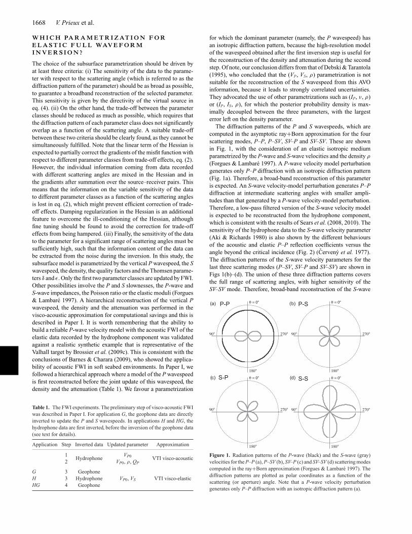
The diffraction patterns of the P and S wavespeeds, which arecomputed in the asymptotic ray+Born approximation for the fourscattering modes, P–P, P–SV, SV–P and SV–SV. These are shownin Fig. 1, with the consideration of an elastic isotropic mediumparametrized by the P-wave and S-wave velocities and the density ρ

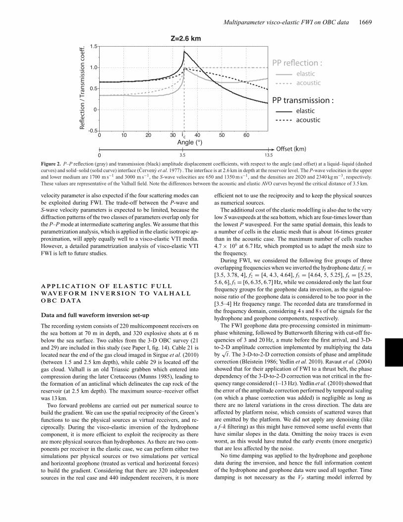
(Forgues & Lambare 1997). A P-wave velocity model perturbationgenerates only P–P diffraction with an isotropic diffraction pattern(Fig. 1a). Therefore, a broad-band reconstruction of this parameteris expected. An S-wave velocity-model perturbation generates P–Pdiffraction at intermediate scattering angles with smaller ampli-tudes than that generated by a P-wave velocity-model perturbation.Therefore, a low-pass filtered version of the S-wave velocity modelis expected to be reconstructed from the hydrophone component,which is consistent with the results of Sears et al. (2008, 2010). Thesensitivity of the hydrophone data to the S-wave velocity parameter(Aki & Richards 1980) is also shown by the different behavioursof the acoustic and elastic P–P reflection coefficients versus theangle beyond the critical incidence (Fig. 2) (Cerveny et al. 1977).The diffraction patterns of the S-wave velocity parameters for thelast three scattering modes (P–SV, SV–P and SV–SV) are shown inFigs 1(b)–(d). The union of these three diffraction patterns coversthe full range of scattering angles, with higher sensitivity of theSV–SV mode. Therefore, broad-band reconstruction of the S-wave

Figure 1. Radiation patterns of the P-wave (black) and the S-wave (gray)velocities for the P–P (a), P–SV (b), SV–P (c) and SV–SV (d) scattering modescomputed in the ray+Born approximation (Forgues & Lambare 1997). Thediffraction patterns are plotted as polar coordinates as a function of thescattering (or aperture) angle. Note that a P-wave velocity perturbationgenerates only P–P diffraction with an isotropic diffraction pattern (a).

Multiparameter visco-elastic FWI on OBC data 1669

Figure 2. P–P reflection (gray) and transmission (black) amplitude displacement coefficients, with respect to the angle (and offset) at a liquid–liquid (dashedcurves) and solid–solid (solid curve) interface (Cerveny et al. 1977) . The interface is at 2.6 km in depth at the reservoir level. The P-wave velocities in the upperand lower medium are 1700 m s−1 and 3000 m s−1, the S-wave velocities are 650 and 1350 m s−1, and the densities are 2020 and 2340 kg m−3, respectively.These values are representative of the Valhall field. Note the differences between the acoustic and elastic AVO curves beyond the critical distance of 3.5 km.

velocity parameter is also expected if the four scattering modes canbe exploited during FWI. The trade-off between the P-wave andS-wave velocity parameters is expected to be limited, because thediffraction patterns of the two classes of parameters overlap only forthe P–P mode at intermediate scattering angles. We assume that thisparametrization analysis, which is applied in the elastic isotropic ap-proximation, will apply equally well to a visco-elastic VTI media.However, a detailed parametrization analysis of visco-elastic VTIFWI is left to future studies.

A P P L I C AT I O N O F E L A S T I C F U L LWAV E F O R M I N V E R S I O N T O VA L H A L LO B C DATA

Data and full waveform inversion set-up

The recording system consists of 220 multicomponent receivers onthe sea bottom at 70 m in depth, and 320 explosive shots at 6 mbelow the sea surface. Two cables from the 3-D OBC survey (21and 29) are included in this study (see Paper I, fig. 14). Cable 21 islocated near the end of the gas cloud imaged in Sirgue et al. (2010)(between 1.5 and 2.5 km depth), while cable 29 is located off thegas cloud. Valhall is an old Triassic grabben which entered intocompression during the later Cretaceous (Munns 1985), leading tothe formation of an anticlinal which delineates the cap rock of thereservoir (at 2.5 km depth). The maximum source–receiver offsetwas 13 km.

Two forward problems are carried out per numerical source tobuild the gradient. We can use the spatial reciprocity of the Green’sfunctions to use the physical sources as virtual receivers, and re-ciprocally. During the visco-elastic inversion of the hydrophonecomponent, it is more efficient to exploit the reciprocity as thereare more physical sources than hydrophones. As there are two com-ponents per receiver in the elastic case, we can perform either twosimulations per physical sources or two simulations per verticaland horizontal geophone (treated as vertical and horizontal forces)to build the gradient. Considering that there are 320 independentsources in the real case and 440 independent receivers, it is more

efficient not to use the reciprocity and to keep the physical sourcesas numerical sources.

The additional cost of the elastic modelling is also due to the verylow S wavespeeds at the sea bottom, which are four-times lower thanthe lowest P wavespeed. For the same spatial domain, this leads toa number of cells in the elastic mesh that is about 16-times greaterthan in the acoustic case. The maximum number of cells reaches4.7 × 106 at 6.7 Hz, which prompted us to adapt the mesh size tothe frequency.

During FWI, we considered the following five groups of threeoverlapping frequencies when we inverted the hydrophone data: f1 =[3.5, 3.78, 4], f2 = [4, 4.3, 4.64], f3 = [4.64, 5, 5.25], f4 = [5.25,5.6, 6], f5 = [6, 6.35, 6.7] Hz, while we considered only the last fourfrequency groups for the geophone data inversion, as the signal-to-noise ratio of the geophone data is considered to be too poor in the[3.5–4] Hz frequency range. The recorded data are transformed inthe frequency domain, considering 4 s and 8 s of the signals for thehydrophone and geophone components, respectively.

The FWI geophone data pre-processing consisted in minimum-phase whitening, followed by Butterworth filtering with cut-off fre-quencies of 3 and 20 Hz, a mute before the first arrival, and 3-D-to-2-D amplitude correction implemented by multiplying the databy

√t . The 3-D-to-2-D correction consists of phase and amplitude

correction (Bleistein 1986; Yedlin et al. 2010). Ravaut et al. (2004)showed that for their application of FWI to a thrust belt, the phasedependency of the 3-D-to-2-D correction was not critical in the fre-quency range considered (1–13 Hz). Yedlin et al. (2010) showed thatthe error of the amplitude correction performed by temporal scaling(on which a phase correction was added) is negligible as long asthere are no lateral variations in the cross direction. The data areaffected by platform noise, which consists of scattered waves thatare emitted by the platform. We did not apply any denoising (likea f–k filtering) as this might have removed some useful events thathave similar slopes in the data. Omitting the noisy traces is evenworst, as this would have muted the early events (more energetic)that are less affected by the noise.

No time damping was applied to the hydrophone and geophonedata during the inversion, and hence the full information contentof the hydrophone and geophone data were used all together. Timedamping is not necessary as the VP starting model inferred by

1670 V. Prieux et al.

visco-acoustic FWI already explains the acoustic wavefield, and weare interested in extracting information from the P-to-S convertedwaves, which are late arrivals. Moreover, no gain with offset wasapplied to the data during the inversion (Wd = I in eq. 1). The L-BFGS optimization performed less than 10 iterations per frequencygroup, although the maximum number of iterations was set to 25.Our stopping criteria forces the inversion to stop as soon as themaximum velocity perturbation is lower than 10−3 per cent of thevelocity of the starting model at the position of maximum velocity.A source wavelet per shot gather was estimated at each iterationof the hydrophone and geophone data by solving a linear inverseproblem (see eq. 17 in Pratt 1999).

The standard errors σ i, which are used in the weighting matricesWmi , in eq. (2), are set to 1, because we normalize the subsurfaceparameters by their mean values (see Paper I). The damping factorsλi are defined according to the amplitude of the partial derivativeof the wavefields with respect to the parameter classes, which canbe assessed from the diagonal terms of the approximate Hessian,eq. (5); namely, the auto-correlation of the partial derivative wave-fields. The maximum value of the approximate Hessian associatedwith the vertical P wavespeed is on average four-times higher thanthat associated with the S wavespeed for all of the tests, and there-fore we use a damping value for the S wavespeed that is four-timessmaller than that used for the vertical P wavespeed. We will showin the following that this tuning allows reasonable agreement to beachieved between the FWI models and the sonic logs. The dampingvalues used for the vertical P and S wavespeeds are outlined inTable 2.

Table 2. The FWI set-up. The inversiondampings λ for each parameter class.

Parameter λ

VP0 (m s−1) 4 × 10−8

ρ (kg m−3) 4 × 10−8

QP 4 × 10−10

VS (m s−1) 1 × 10−8

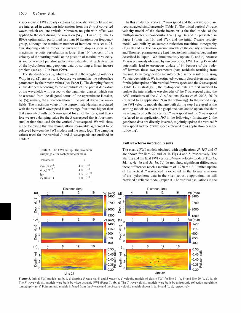
In this study, the vertical P wavespeed and the S wavespeed arereconstructed simultaneously (Table 1). The initial vertical P-wavevelocity model of the elastic inversion is the final model of themultiparameter visco-acoustic FWI (Fig. 3a and d) presented inPaper I (their figs 16h and 17e), and the initial S-wave velocitymodel was built by anisotropic reflection traveltime tomography(Figs 3b and e). The background models of the density, attenuationand Thomsen parameters are kept fixed to their initial values, and aredescribed in Paper I. We simultaneously update VP and VS becauseVP was previously obtained by visco-acoustic FWI. Fixing VP wouldpotentially lead to erroneous update of VS because of the trade-off between these two parameters (data residuals resulting frommissing VP heterogeneities are interpreted as the result of missingVS heterogeneities). We investigated two main data-driven strategiesfor the joint update of the vertical P wavespeed and the S wavespeed(Table 1): in strategy 1, the hydrophone data are first inverted toupdate the intermediate wavelengths of the S wavespeed using theAVO variations of the P–P reflections (Sears et al. 2008, 2010)(referred to as application H in the following). In the second step,the FWI velocity models that are built during step 1 are used as thestarting models to invert the geophone data and to update the shortwavelengths of both the vertical P wavespeed and the S wavespeed(referred to as application HG in the following). In strategy 2, thegeophone data are directly inverted, to jointly update the vertical Pwavespeed and the S wavespeed (referred to as application G in thefollowing).

Full waveform inversion results

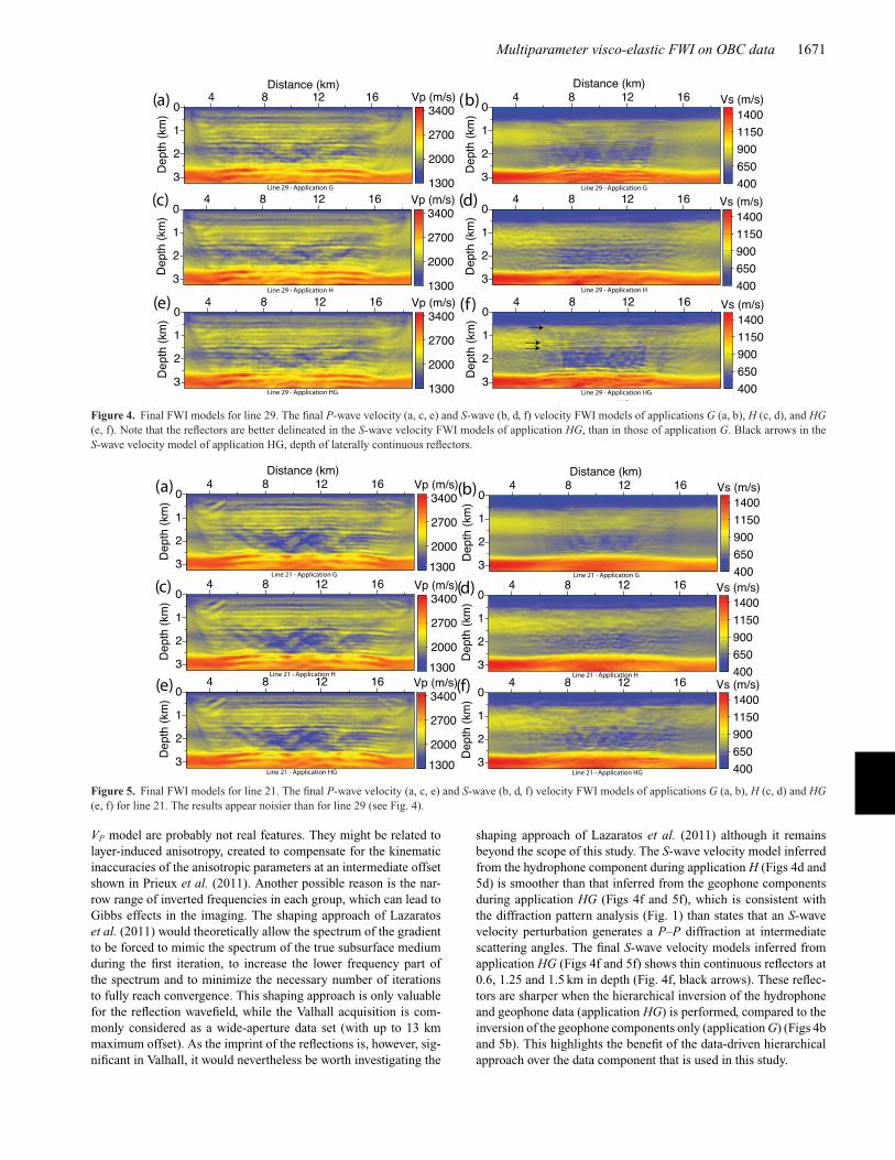
The elastic FWI models obtained with applications H, HG and Gare shown for lines 29 and 21 in Figs 4 and 5, respectively. Thestarting and the final FWI vertical P-wave velocity models (Figs 3a,3d, 4a, 4c, 4e and 5a, 5c, 5e) do not show significant differences;these differences reach a maximum of ±250 m s−1. Limited updateof the vertical P wavespeed is expected, as the former inversionof the hydrophone data in the visco-acoustic approximation stillprovided a reliable model (Paper I). The vertical oscillations in the

Figure 3. Initial FWI models. (a, b, d, e) Starting P-wave (a, d) and S-wave (b, e) velocity models of elastic FWI for line 21 (a, b) and line 29 (d, e). (a, d)The P-wave velocity models were built by visco-acoustic FWI (Paper I). (b, e) The S-wave velocity models were built by anisotropic reflection traveltimetomography. (c, f) Poisson ratio models inferred from the P-wave and the S-wave velocity models shown in (a, b) and (d, e), respectively.

Multiparameter visco-elastic FWI on OBC data 1671

Figure 4. Final FWI models for line 29. The final P-wave velocity (a, c, e) and S-wave (b, d, f) velocity FWI models of applications G (a, b), H (c, d), and HG(e, f). Note that the reflectors are better delineated in the S-wave velocity FWI models of application HG, than in those of application G. Black arrows in theS-wave velocity model of application HG, depth of laterally continuous reflectors.

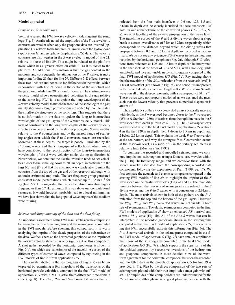
Figure 5. Final FWI models for line 21. The final P-wave velocity (a, c, e) and S-wave (b, d, f) velocity FWI models of applications G (a, b), H (c, d) and HG(e, f) for line 21. The results appear noisier than for line 29 (see Fig. 4).

VP model are probably not real features. They might be related tolayer-induced anisotropy, created to compensate for the kinematicinaccuracies of the anisotropic parameters at an intermediate offsetshown in Prieux et al. (2011). Another possible reason is the nar-row range of inverted frequencies in each group, which can lead toGibbs effects in the imaging. The shaping approach of Lazaratoset al. (2011) would theoretically allow the spectrum of the gradientto be forced to mimic the spectrum of the true subsurface mediumduring the first iteration, to increase the lower frequency part ofthe spectrum and to minimize the necessary number of iterationsto fully reach convergence. This shaping approach is only valuablefor the reflection wavefield, while the Valhall acquisition is com-monly considered as a wide-aperture data set (with up to 13 kmmaximum offset). As the imprint of the reflections is, however, sig-nificant in Valhall, it would nevertheless be worth investigating the

shaping approach of Lazaratos et al. (2011) although it remainsbeyond the scope of this study. The S-wave velocity model inferredfrom the hydrophone component during application H (Figs 4d and5d) is smoother than that inferred from the geophone componentsduring application HG (Figs 4f and 5f), which is consistent withthe diffraction pattern analysis (Fig. 1) than states that an S-wavevelocity perturbation generates a P–P diffraction at intermediatescattering angles. The final S-wave velocity models inferred fromapplication HG (Figs 4f and 5f) shows thin continuous reflectors at0.6, 1.25 and 1.5 km in depth (Fig. 4f, black arrows). These reflec-tors are sharper when the hierarchical inversion of the hydrophoneand geophone data (application HG) is performed, compared to theinversion of the geophone components only (application G) (Figs 4band 5b). This highlights the benefit of the data-driven hierarchicalapproach over the data component that is used in this study.

1672 V. Prieux et al.

Model appraisal

Comparison with sonic logs

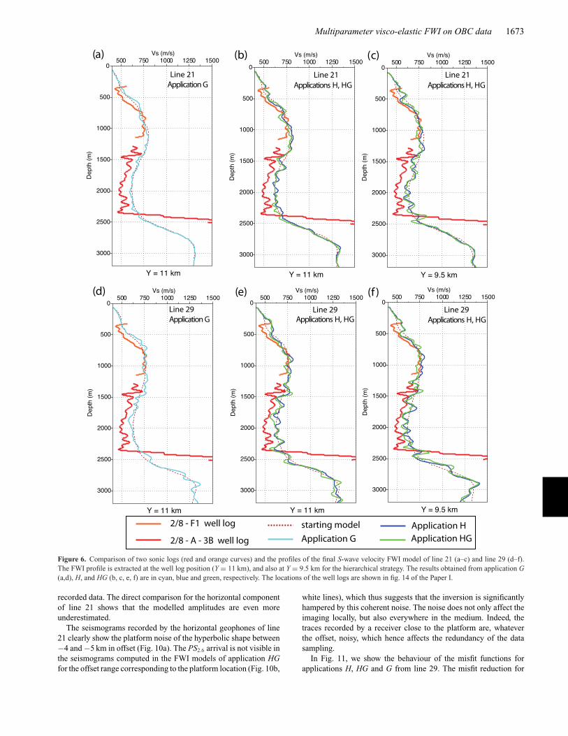
We first assessed the FWI S-wave velocity models against the soniclogs (Fig. 6). As already noted, the amplitudes of the S-wave velocitycontrasts are weaker when only the geophone data are inverted (ap-plication G), relative to the hierarchical inversion of the hydrophone(application H) and geophone (application HG) data. The velocitycontrasts are also weaker in the S-wave velocity model of line 21,relative to those of line 29. This might be related to the platformnoise which has a greater effect on cable 21 as it is closer to theplatform. An additional explanation is that the gas content in themedium, and consequently the attenuation of the P waves, is moreimportant for line 21 than for line 29. Different 3-D effects betweenthese two lines are another cause for differences in the results, whichis consistent with line 21 being in the centre of the anticlinal andthe gas cloud, while line 29 is more off-centre. The starting S-wavevelocity model shows overestimated velocities in the gas relativeto the sonic log. FWI fails to update the long wavelengths of theS-wave velocity model to match the trend of the sonic log in the gas;mainly short-wavelength perturbations are added by FWI, to matchthe small-scale structures of the sonic logs. This suggests that thereis no information in the data to update the long-to-intermediatewavelengths of the gas layers of the S-wave velocity model. Thislack of constraints on the long wavelengths of the S-wave velocitystructure can be explained by the shorter propagated S wavelengths,relative to the P counterparts and by the narrow range of scatter-ing angles over which the P-to-S converted waves are recorded.Moreover, at these depths, the target is poorly illuminated by theP diving waves and the P long-spread reflections, which wouldhave contributed to the reconstruction of the long-to-intermediatewavelengths of the S-wave velocity model during application H.Nevertheless, we note that the elastic inversion tends to set veloci-ties closer to the sonic log down to 700 m depth, in particular in theFigs 6(e) and (f), and that the inversion was clearly able to mark thecontrasts from the top of the gas and of the reservoir, although withan under-estimated amplitude. The last frequency group generatedconsistent model perturbations, which reached up to 135 m s−1 forVS (line 29). This suggested that we can continue inverting higherfrequencies than 6.7 Hz, although this was above our computationalresources. It would, however, probably lead to a local minimum aswe have just shown that the long spatial wavelengths of the mediumwere missing.

Seismic modelling: anatomy of the data and the data fitting

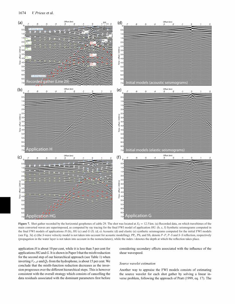
An important assessment of the FWI results relies on the comparisonbetween the recorded seismograms and the seismograms computedin the FWI models. Before showing this comparison, it is worthanalysing the imprint of the elastic properties of the subsurface onthe data. We focus here on the horizontal geophone, as the imprint ofthe S-wave velocity structure is only significant on this component.A shot gather recorded by the horizontal geophones is shown inFig. 7(a), on which are superimposed the traveltime curves of thedifferent types of converted waves computed by ray tracing in theFWI models of line 29 from application HG.

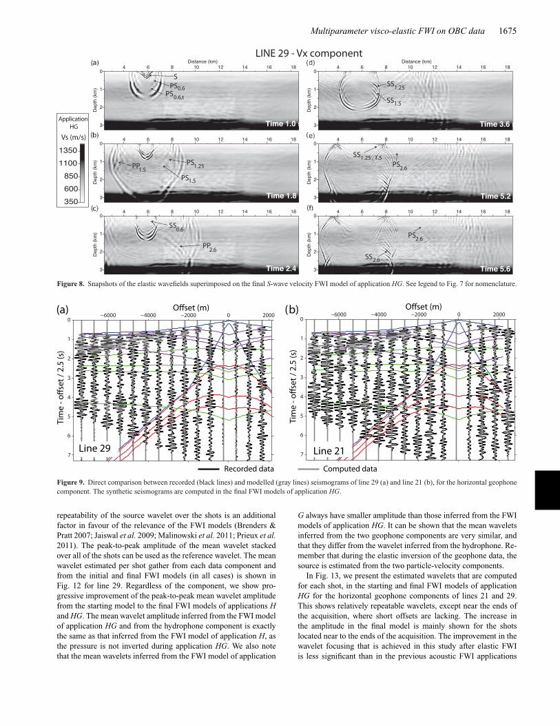
The arrivals labelled in the seismograms of Fig. 7(a) can be in-terpreted by examining a few snapshots of the wavefronts of thehorizontal particle velocities, computed in the final FWI model ofapplication HG with a VTI elastic finite-difference time-domaincode (Fig. 8). The P–P, P–S and S–S converted waves that are

reflected from the four main interfaces at 0.6 km, 1.25, 1.5 and2.6 km in depth can be clearly identified in these snapshots. Ofnote, in our nomenclature of the converted phases (P–P, P–S, S–S), we omit labelling of the P-wave propagation in the water layer.The traveltime curves of the P and S diving waves show a slopebreak at a cross-over distance of 3 km and 2 km, respectively, whichcorresponds to the distance beyond which the diving waves thatpropagate between 0.6 and 1.5 km in depth are recorded as first ar-rivals. We do not see any evidence of S–S waves in the seismogramsrecorded by the horizontal geophone (Fig. 7a), although S–S reflec-tions from reflectors at 1.25 and 1.5 km in depth can be interpretedin the snapshots at the times of 3.6 and 5.2 s, with a non-negligibleamplitude, and they are visible in the seismograms computed in thefinal FWI model of application HG (Fig. 7c). Ray tracing showsthat the traveltime of the SS2.6 reflection (from the reservoir level) is7.8 s at zero offset (not shown in Fig. 7a), and hence it is not presentin the recorded data, as the trace length is 8 s. We also show Scholtewaves on all of the data components, with a wavespeed <350 m s−1.These waves were not properly modelled, as we designed the meshsuch that the lowest velocity that prevents numerical dispersion is400 m s−1.

The amplitudes of the P-to-S converted phases generally increasewith depth, as the S wavespeed becomes closer to the P wavespeed(White & Stephen 1980); this arises from the rapid increase in the Swavespeed with depth (Hoven et al. 1991). The P-wavespeed overS-wavespeed ratio in the final FWI model of application HG is about4 in the first 220 m in depth, then 3 down to 2.5 km in depth, and2 below 2.5 km in depth. This explains the weak P-to-S conversionat the sea bottom, and why the strongest P-to-S conversion occursat the reservoir level, as a ratio of 3 in the tertiary sediments isrelatively high (Mueller et al. 1997).

To compare the recorded and modelled seismograms, we com-pute impulsional seismograms using a Dirac source wavelet withinthe [1–10] Hz frequency range, and we convolve these with thesource wavelet estimated from the corresponding recorded datacomponent, following the expression of Pratt (1999, eq. 17). Wefirst compare the acoustic and elastic seismograms computed in thestarting FWI models of line 29, to highlight the imprint of the Swavespeed on the elastic wavefields (Figs 7d and e). The main dif-ferences between the two sets of seismograms are related to the Sdiving waves and the P-to-S waves with a conversion at 2.6 km indepth. The main arrivals shown in both of the gathers are the P–Preflection from the top and the bottom of the gas layers. However,the PS0.6, PS1.25 and PS1.5 converted waves are not visible in bothsets of seismograms. The elastic seismograms computed in the finalFWI models of application H show an enhanced PS2.6 arrival anda weak PS1.5 wave (Fig. 7b). All of the P-to-S waves that can beinterpreted in the recorded gather are shown in the seismogramscomputed in the final FWI model of application HG, thus confirm-ing that FWI successfully extracts this information (Fig. 7c). TheP-to-S converted arrivals in the seismograms computed in the fi-nal FWI model of application G (Fig. 7f) have smaller amplitudesthan those of the seismograms computed in the final FWI modelof application HG (Fig. 7c), which supports the superiority of thehierarchical approach by successive inversions of the hydrophoneand geophone components. A more detailed view of the wave-form agreement for the horizontal component between the recordedand modelled data in the models of application HG for line 29 isprovided in Fig. 9(a) by the direct comparison of the two sets ofseismograms plotted with their true amplitudes and a gain with off-set. The amplitudes of the computed data are underestimated for theP-to-S arrivals, although we note good phase agreement with the

Multiparameter visco-elastic FWI on OBC data 1673

Figure 6. Comparison of two sonic logs (red and orange curves) and the profiles of the final S-wave velocity FWI model of line 21 (a–c) and line 29 (d–f).The FWI profile is extracted at the well log position (Y = 11 km), and also at Y = 9.5 km for the hierarchical strategy. The results obtained from application G(a,d), H, and HG (b, c, e, f) are in cyan, blue and green, respectively. The locations of the well logs are shown in fig. 14 of the Paper I.

recorded data. The direct comparison for the horizontal componentof line 21 shows that the modelled amplitudes are even moreunderestimated.

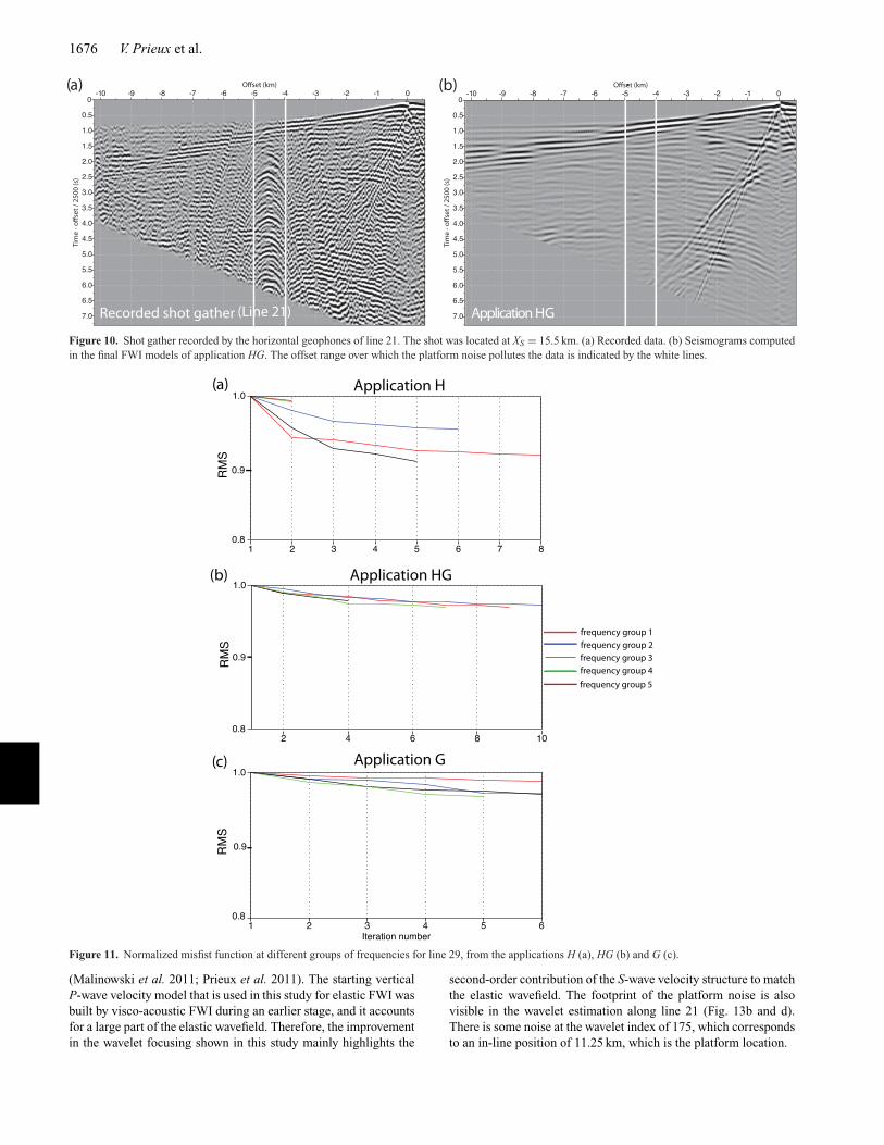
The seismograms recorded by the horizontal geophones of line21 clearly show the platform noise of the hyperbolic shape between−4 and −5 km in offset (Fig. 10a). The PS2.6 arrival is not visible inthe seismograms computed in the FWI models of application HGfor the offset range corresponding to the platform location (Fig. 10b,

white lines), which thus suggests that the inversion is significantlyhampered by this coherent noise. The noise does not only affect theimaging locally, but also everywhere in the medium. Indeed, thetraces recorded by a receiver close to the platform are, whateverthe offset, noisy, which hence affects the redundancy of the datasampling.

In Fig. 11, we show the behaviour of the misfit functions forapplications H, HG and G from line 29. The misfit reduction for

1674 V. Prieux et al.

Figure 7. Shot gather recorded by the horizontal geophones of cable 29. The shot was located at XS = 12.5 km. (a) Recorded data, on which traveltimes of themain converted waves are superimposed, as computed by ray tracing for the final FWI model of application HG. (b, c, f) Synthetic seismograms computed inthe final FWI models of applications H (b), HG (c) and G (f). (d, e) Acoustic (d) and elastic (e) synthetic seismograms computed for the initial FWI models(see Fig. 3d, e) (the S-wave velocity model is not taken into account for acoustic modelling). PPi, PSi and SSi denote P–P, P–S and S–S reflection, respectively(propagation in the water layer is not taken into account in the nomenclature), while the index i denotes the depth at which the reflection takes place.

application H is about 10 per cent, while it is less than 5 per cent forapplications HG and G. It is shown in Paper I that the misfit reductionfor the second step of our hierarchical approach (see Table 1) wheninverting VP, ρ and QP from the hydrophone, is about 15 per cent. Weconclude that the misfit-function reduction decreases as the inver-sion progresses over the different hierarchical steps. This is howeverconsistent with the overall strategy which consists of cancelling thedata residuals associated with the dominant parameters first before

considering secondary effects associated with the influence of theshear wavespeed.

Source wavelet estimation

Another way to appraise the FWI models consists of estimatingthe source wavelet for each shot gather by solving a linear in-verse problem, following the approach of Pratt (1999, eq. 17). The

Multiparameter visco-elastic FWI on OBC data 1675

Figure 8. Snapshots of the elastic wavefields superimposed on the final S-wave velocity FWI model of application HG. See legend to Fig. 7 for nomenclature.

Figure 9. Direct comparison between recorded (black lines) and modelled (gray lines) seismograms of line 29 (a) and line 21 (b), for the horizontal geophonecomponent. The synthetic seismograms are computed in the final FWI models of application HG.

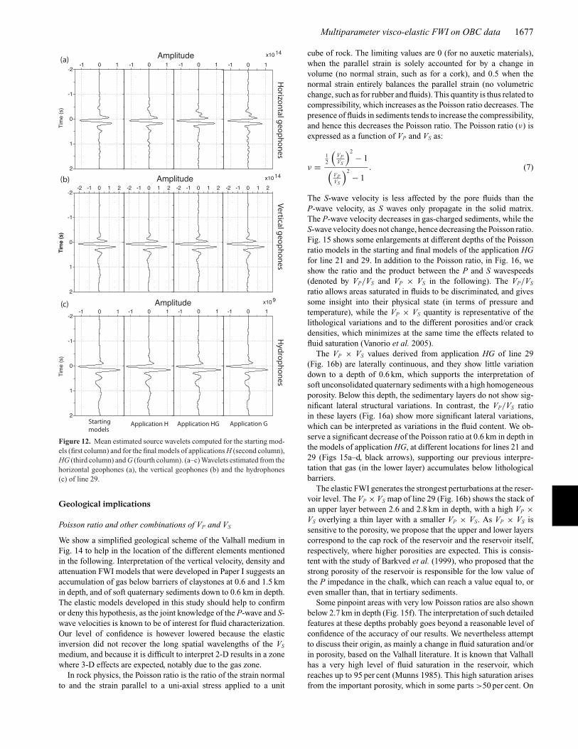
repeatability of the source wavelet over the shots is an additionalfactor in favour of the relevance of the FWI models (Brenders &Pratt 2007; Jaiswal et al. 2009; Malinowski et al. 2011; Prieux et al.2011). The peak-to-peak amplitude of the mean wavelet stackedover all of the shots can be used as the reference wavelet. The meanwavelet estimated per shot gather from each data component andfrom the initial and final FWI models (in all cases) is shown inFig. 12 for line 29. Regardless of the component, we show pro-gressive improvement of the peak-to-peak mean wavelet amplitudefrom the starting model to the final FWI models of applications Hand HG. The mean wavelet amplitude inferred from the FWI modelof application HG and from the hydrophone component is exactlythe same as that inferred from the FWI model of application H, asthe pressure is not inverted during application HG. We also notethat the mean wavelets inferred from the FWI model of application

G always have smaller amplitude than those inferred from the FWImodels of application HG. It can be shown that the mean waveletsinferred from the two geophone components are very similar, andthat they differ from the wavelet inferred from the hydrophone. Re-member that during the elastic inversion of the geophone data, thesource is estimated from the two particle-velocity components.

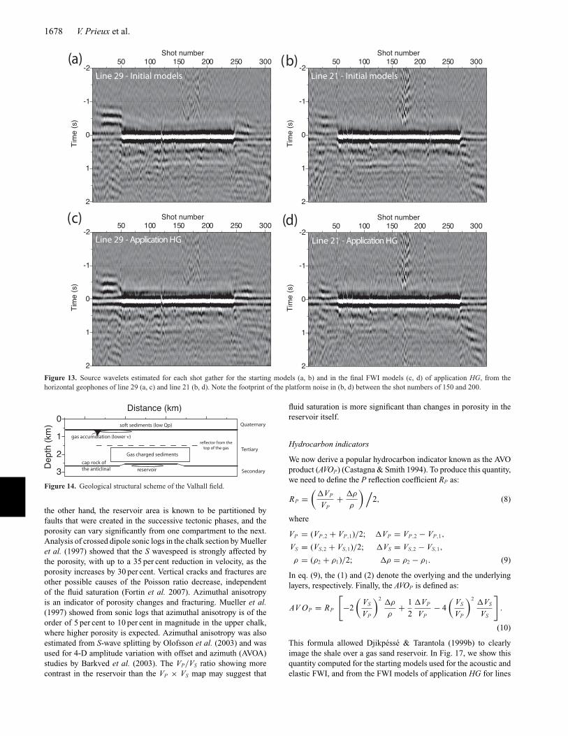
In Fig. 13, we present the estimated wavelets that are computedfor each shot, in the starting and final FWI models of applicationHG for the horizontal geophone components of lines 21 and 29.This shows relatively repeatable wavelets, except near the ends ofthe acquisition, where short offsets are lacking. The increase inthe amplitude in the final model is mainly shown for the shotslocated near to the ends of the acquisition. The improvement in thewavelet focusing that is achieved in this study after elastic FWIis less significant than in the previous acoustic FWI applications

1676 V. Prieux et al.

Figure 10. Shot gather recorded by the horizontal geophones of line 21. The shot was located at XS = 15.5 km. (a) Recorded data. (b) Seismograms computedin the final FWI models of application HG. The offset range over which the platform noise pollutes the data is indicated by the white lines.

Figure 11. Normalized misfist function at different groups of frequencies for line 29, from the applications H (a), HG (b) and G (c).

(Malinowski et al. 2011; Prieux et al. 2011). The starting verticalP-wave velocity model that is used in this study for elastic FWI wasbuilt by visco-acoustic FWI during an earlier stage, and it accountsfor a large part of the elastic wavefield. Therefore, the improvementin the wavelet focusing shown in this study mainly highlights the

second-order contribution of the S-wave velocity structure to matchthe elastic wavefield. The footprint of the platform noise is alsovisible in the wavelet estimation along line 21 (Fig. 13b and d).There is some noise at the wavelet index of 175, which correspondsto an in-line position of 11.25 km, which is the platform location.

Multiparameter visco-elastic FWI on OBC data 1677

Figure 12. Mean estimated source wavelets computed for the starting mod-els (first column) and for the final models of applications H (second column),HG (third column) and G (fourth column). (a–c) Wavelets estimated from thehorizontal geophones (a), the vertical geophones (b) and the hydrophones(c) of line 29.

Geological implications

Poisson ratio and other combinations of VP and VS

We show a simplified geological scheme of the Valhall medium inFig. 14 to help in the location of the different elements mentionedin the following. Interpretation of the vertical velocity, density andattenuation FWI models that were developed in Paper I suggests anaccumulation of gas below barriers of claystones at 0.6 and 1.5 kmin depth, and of soft quaternary sediments down to 0.6 km in depth.The elastic models developed in this study should help to confirmor deny this hypothesis, as the joint knowledge of the P-wave and S-wave velocities is known to be of interest for fluid characterization.Our level of confidence is however lowered because the elasticinversion did not recover the long spatial wavelengths of the VS

medium, and because it is difficult to interpret 2-D results in a zonewhere 3-D effects are expected, notably due to the gas zone.

In rock physics, the Poisson ratio is the ratio of the strain normalto and the strain parallel to a uni-axial stress applied to a unit

cube of rock. The limiting values are 0 (for no auxetic materials),when the parallel strain is solely accounted for by a change involume (no normal strain, such as for a cork), and 0.5 when thenormal strain entirely balances the parallel strain (no volumetricchange, such as for rubber and fluids). This quantity is thus related tocompressibility, which increases as the Poisson ratio decreases. Thepresence of fluids in sediments tends to increase the compressibility,and hence this decreases the Poisson ratio. The Poisson ratio (ν) isexpressed as a function of VP and VS as:

ν =12

(VPVS

)2− 1(

VPVS

)2− 1

. (7)

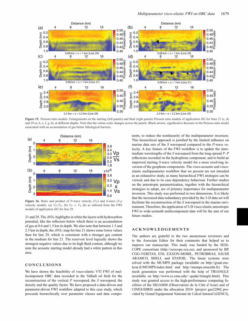
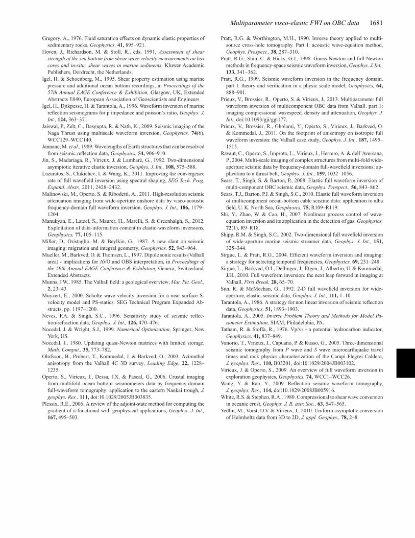
The S-wave velocity is less affected by the pore fluids than theP-wave velocity, as S waves only propagate in the solid matrix.The P-wave velocity decreases in gas-charged sediments, while theS-wave velocity does not change, hence decreasing the Poisson ratio.Fig. 15 shows some enlargements at different depths of the Poissonratio models in the starting and final models of the application HGfor line 21 and 29. In addition to the Poisson ratio, in Fig. 16, weshow the ratio and the product between the P and S wavespeeds(denoted by VP/VS and VP × VS in the following). The VP/VS

ratio allows areas saturated in fluids to be discriminated, and givessome insight into their physical state (in terms of pressure andtemperature), while the VP × VS quantity is representative of thelithological variations and to the different porosities and/or crackdensities, which minimizes at the same time the effects related tofluid saturation (Vanorio et al. 2005).

The VP × VS values derived from application HG of line 29(Fig. 16b) are laterally continuous, and they show little variationdown to a depth of 0.6 km, which supports the interpretation ofsoft unconsolidated quaternary sediments with a high homogeneousporosity. Below this depth, the sedimentary layers do not show sig-nificant lateral structural variations. In contrast, the VP/VS ratioin these layers (Fig. 16a) show more significant lateral variations,which can be interpreted as variations in the fluid content. We ob-serve a significant decrease of the Poisson ratio at 0.6 km in depth inthe models of application HG, at different locations for lines 21 and29 (Figs 15a–d, black arrows), supporting our previous interpre-tation that gas (in the lower layer) accumulates below lithologicalbarriers.

The elastic FWI generates the strongest perturbations at the reser-voir level. The VP × VS map of line 29 (Fig. 16b) shows the stack ofan upper layer between 2.6 and 2.8 km in depth, with a high VP ×VS overlying a thin layer with a smaller VP × VS. As VP × VS issensitive to the porosity, we propose that the upper and lower layerscorrespond to the cap rock of the reservoir and the reservoir itself,respectively, where higher porosities are expected. This is consis-tent with the study of Barkved et al. (1999), who proposed that thestrong porosity of the reservoir is responsible for the low value ofthe P impedance in the chalk, which can reach a value equal to, oreven smaller than, that in tertiary sediments.

Some pinpoint areas with very low Poisson ratios are also shownbelow 2.7 km in depth (Fig. 15f). The interpretation of such detailedfeatures at these depths probably goes beyond a reasonable level ofconfidence of the accuracy of our results. We nevertheless attemptto discuss their origin, as mainly a change in fluid saturation and/orin porosity, based on the Valhall literature. It is known that Valhallhas a very high level of fluid saturation in the reservoir, whichreaches up to 95 per cent (Munns 1985). This high saturation arisesfrom the important porosity, which in some parts >50 per cent. On

1678 V. Prieux et al.

Figure 13. Source wavelets estimated for each shot gather for the starting models (a, b) and in the final FWI models (c, d) of application HG, from thehorizontal geophones of line 29 (a, c) and line 21 (b, d). Note the footprint of the platform noise in (b, d) between the shot numbers of 150 and 200.

Figure 14. Geological structural scheme of the Valhall field.

the other hand, the reservoir area is known to be partitioned byfaults that were created in the successive tectonic phases, and theporosity can vary significantly from one compartment to the next.Analysis of crossed dipole sonic logs in the chalk section by Muelleret al. (1997) showed that the S wavespeed is strongly affected bythe porosity, with up to a 35 per cent reduction in velocity, as theporosity increases by 30 per cent. Vertical cracks and fractures areother possible causes of the Poisson ratio decrease, independentof the fluid saturation (Fortin et al. 2007). Azimuthal anisotropyis an indicator of porosity changes and fracturing. Mueller et al.(1997) showed from sonic logs that azimuthal anisotropy is of theorder of 5 per cent to 10 per cent in magnitude in the upper chalk,where higher porosity is expected. Azimuthal anisotropy was alsoestimated from S-wave splitting by Olofsson et al. (2003) and wasused for 4-D amplitude variation with offset and azimuth (AVOA)studies by Barkved et al. (2003). The VP/VS ratio showing morecontrast in the reservoir than the VP × VS map may suggest that

fluid saturation is more significant than changes in porosity in thereservoir itself.

Hydrocarbon indicators

We now derive a popular hydrocarbon indicator known as the AVOproduct (AVOP) (Castagna & Smith 1994). To produce this quantity,we need to define the P reflection coefficient RP as:

RP =(

�VP

VP+ �ρ

ρ

) /2, (8)

where

VP = (VP,2 + VP,1)/2; �VP = VP,2 − VP,1,

VS = (VS,2 + VS,1)/2; �VS = VS,2 − VS,1,

ρ = (ρ2 + ρ1)/2; �ρ = ρ2 − ρ1. (9)

In eq. (9), the (1) and (2) denote the overlying and the underlyinglayers, respectively. Finally, the AVOP is defined as:

AV OP = RP

[−2

(VS

VP

)2�ρ

ρ+ 1

2

�VP

VP− 4

(VS

VP

)2�VS

VS

].

(10)

This formula allowed Djikpesse & Tarantola (1999b) to clearlyimage the shale over a gas sand reservoir. In Fig. 17, we show thisquantity computed for the starting models used for the acoustic andelastic FWI, and from the FWI models of application HG for lines

Multiparameter visco-elastic FWI on OBC data 1679

Figure 15. Poisson ratio models. Enlargements on the starting (left panels) and final (right panels) Poisson ratio models of application HG for lines 21 (c, d)and 29 (a, b, e, f, g, h), at different depths. Note that the colour scale changes across the panels. Black arrows, significative decrease in the Poisson ratio modelassociated with an accumulation of gas below lithological barriers.

Figure 16. Ratio and product of P-wave velocity (VP) and S-wave (VS)velocity models. (a) VP/VS. (b) VP × VS (b) as inferred from the FWImodels of application HG for line 29.

21 and 29. The AVOP highlights in white the layers with hydrocarbonpotential, like the reflectors below which there is an accumulationof gas at 0.6 and 1.5 km in depth. We also note that between 1.5 and2.5 km in depth, the AVOP map for line 21 shows some lower valuesthan for line 29, which is consistent with a stronger gas contentin the medium for line 21. The reservoir level logically shows thestrongest negative values due to its high fluid content, although wenote the acoustic starting model already had a white pattern in thisarea.

C O N C LU S I O N S

We have shown the feasibility of visco-elastic VTI FWI of mul-ticomponent OBC data recorded in the Valhall oil field for thereconstruction of the vertical P wavespeed, the S wavespeed, thedensity and the quality factor. We have proposed a data-driven andparameter-driven FWI workflow adapted to this case study, whichproceeds hierarchically over parameter classes and data compo-

nents, to reduce the nonlinearity of the multiparameter inversion.This hierarchical approach is justified by the limited influence onmarine data sets of the S wavespeed compared to the P-wave ve-locity. A key feature of the FWI workflow is to update the inter-mediate wavelengths of the S wavespeed from the long-spread P–Preflections recorded on the hydrophone component, and to build animproved starting S-wave velocity model for a more resolving in-version of the geophone components. The visco-acoustic and visco-elastic multiparameter workflow that we present are not intendedas an exhaustive study, as many hierarchical FWI strategies can beviewed, and due to its case dependency behaviour. Further studieson the anisotropic parametrization, together with the hierarchicalstrategies to adopt, are of primary importance for multiparameterinversion. This study was performed in two dimensions. It is likelythat the increased data redundancy provided by the 3-D data set willfacilitate the reconstruction of the S wavespeed in the marine envi-ronment. Therefore, the application of 3-D visco-elastic anisotropicFWI to wide-azimuth multicomponent data will be the aim of ourfuture studies.

A C K N OW L E D G E M E N T S

The authors are grateful to the two anonymous reviewers andto the Associate Editor for their comments that helped us toimprove our manuscript. This study was funded by the SEIS-COPE consortium (http://seiscope.oca.eu), and sponsored by BP,CGG-VERITAS, ENI, EXXON-MOBIL, PETROBRAS, SAUDIARAMCO, SHELL and STATOIL. The linear systems weresolved with the MUMPS package (available on http://graal.ens-lyon.fr/MUMPS/index.html and http://mumps.enseeiht.fr). Themesh generation was performed with the help of TRIANGLE(available on http://www.cs.cmu.edu/∼quake/triangle.html). Thisstudy was granted access to the high-performance computing fa-cilities of the SIGAMM (Observatoire de la Cote d’Azur) and ofCINES/IDRIS under the allocation 2010- [project gao2280] pro-vided by Grand Equipement National de Calcul Intensif (GENCI),

1680 V. Prieux et al.

Figure 17. AVO product (see text for details). (a, b) The AVOP computed inthe initial acoustic (a) and elastic (b) models of line 29. The initial acousticmodels are shown in Paper I. The initial elastic models are shown in Fig. 3.(c, d) The AVOP computed in the final FWI models of application HG forline 29 (c) and 21 (d).

and we gratefully acknowledge both of these facilities and the sup-port of their staff. We also thank BP Norge AS and their Valhallpartner Hess Norge AS, for allowing access to the Valhall data setas well as to the well-log velocities.

R E F E R E N C E S

Aki, K. & Richards, P., 1980. Quantitative Seismology: Theory and Methods,W. H. Freeman & Co, New York.

Barkved, O., Mueller, M. & Thomsen, L., 1999. Vector interpretation ofthe valhall 3d/4c obs dataset, in Proceedings of the 61th Annual EAGEConference & Exhibition, Helsinki, Finland, Extended Abstracts.

Barkved, O., Buer, K., Halleland, K., Kjelstadli, R., Kleppan, T. & Kris-tiansen, T., 2003. 4D seismic response or primary production and wasteinjection at the valhall field, in Proceedings of the 65th Annual EAGEConference & Exhibition, Stavanger, Extended Abstracts.

Barnes, C. & Charara, M., 2009. The domain of applicability of acoustic full-waveform inversion for marine seismic data, Geophysics, 74, WCC91–WCC103.

Baumstein, A., Ross, W. & Lee, S., 2011. Simultaneous source elastic inver-sion of surface waves, in Proceedings of the 73rd EAGE Annual Confer-ence and Exhibition, Expanded Abstracts, C040, European Associationof Geoscientists and Engineers.

Bleistein, N., 1986. Two and one half dimensional in plane wave propagation,Geophys. Prospect., 34, 686–703.

Brenders, A.J. & Pratt, R.G., 2007. Full waveform tomography for litho-spheric imaging: results from a blind test in a realistic crustal model,Geophys. J. Int., 168, 133–151.

Brossier, R., Operto, S. & Virieux, J., 2009a. 2D elastic frequency-domainfull-waveform inversion for imaging complex onshore structures, Pro-ceedings of the 71th Annual EAGE Conference & Exhibition, Amsterdam,Expanded Abstracts, U019, European Association of Geoscientists andEngineers.

Brossier, R., Operto, S. & Virieux, J., 2009b. Seismic imaging of com-plex onshore structures by 2D elastic frequency-domain full-waveforminversion, Geophysics, 74, WCC105–WCC118.

Brossier, R., Operto, S. & Virieux, J., 2009c. Two-dimensional seismicimaging of the Valhall model from synthetic OBC data by frequency-domain elastic full-waveform inversion, SEG Tech. Prog. Expand. Abstr.,28, 2293–2297.

Brossier, R., Gholami, Y., Virieux, J. & Operto, S., 2010a. 2D frequency-domain seismic wave modeling in VTI media based on a hp-adaptivediscontinuous galerkin method, in Proceedings of the 72nd Annual Inter-national Meeting, Expanded Abstracts, C046, European Association ofGeoscientists and Engineers.

Brossier, R., Operto, S. & Virieux, J., 2010b. Which data residual norm forrobust elastic frequency-domain full waveform inversion? Geophysics,75, R37–R46.

Brossier, R., 2011. Two-dimensional frequency-domain visco-elastic fullwaveform inversion: parallel algorithms, optimization and performance,Comput. Geosci., 37, 444–455.

Bunks, C., Salek, F.M., Zaleski, S. & Chavent, G., 1995. Multiscale seismicwaveform inversion, Geophysics, 60, 1457–1473.

Castagna, J. & Smith, S., 1994. Comparison of avo indicators: a modelingstudy, Geophysics, 59, 1849–1855.

Cerveny, V., Molotkov, I.A. & Psencik, I., 1977. Ray Method in Seismology,Charles University Press, Prague.

Chavent, G., 2009. Nonlinear Least Squares for Inverse Problems, SpringerDordrecht, Heidelberg, London, New York.

Crase, E., Pica, A., Noble, M., McDonald, J. & Tarantola, A., 1990. Ro-bust elastic non-linear waveform inversion: application to real data, Geo-physics, 55, 527–538.

Crase, E., Wideman, C., Noble, M. & Tarantola, A., 1992. Nonlinear elasticinversion of land seismic reflection data, J. geophys. Res., 97, 4685–4705.

Debski, W. & Tarantola, A., 1995. Information on elastic parameters ob-tained from amplitude of reflected waves, Geophysics, 60, 1426–1436.

Djikpesse, H.A. & Tarantola, A., 1999a. Multiparameter l1 norm waveformfitting: interpretation of gulf of mexico reflection seismograms, Geo-physics, 64, 1023–1035.

Djikpesse, H.A. & Tarantola, A., 1999b. Multiparameter l1 norm wave-form fitting: interpretation of gulf of mexico reflection seismograms,Geophysics, 64, 1023–1035.

Domenico, S.N., 1984. Rock lithology and porosity determination fromshear and compressional wave velocity, Geophysics, 49, 1188–1195.

Forgues, E. & Lambare, G., 1997. Parameterization study for acoustic andelastic ray+born inversion, J. Seism. Explor., 6, 253–278.

Fortin, J., Gueguen, Y. & Schubnel, A., 2007. Effects of pore collapse andgrain crushing on ultrasonic velocities and Vp/Vs, J. geophys. Res., 112,B08207, doi:10.1029/2005JB004005.

Freudenreich, Y., Singh, S. & Barton, P., 2001. Sub-basalt imaging usinga full elastic wavefield inversion scheme, in Proceedings of the 63thAnnual EAGE Conference & Exhibition, Amsterdam, Extended Abstracts,European Association of Geoscientists and Engineers.

Greenhalgh, S., Zhou, B. & Green, A., 2006. Solutions, algorithms and inter-relations for local minimization search geophysical inversion, J. Geophys.Eng., 3, 101–113.

Multiparameter visco-elastic FWI on OBC data 1681

Gregory, A., 1976. Fluid saturation effects on dynamic elastic properties ofsedimentary rocks, Geophysics, 41, 895–921.

Hoven, J., Richardson, M. & Stoll, R., eds. 1991, Assessment of shearstrength of the sea bottom from shear wave velocity measurements on boxcores and in-situ: shear waves in marine sediments, Kluwer AcademicPublishers, Dordrecht, the Netherlands.

Igel, H. & Schoenberg, M., 1995. Shear property estimation using marinepressure and additional ocean bottom recordings, in Proceedings of the57th Annual EAGE Conference & Exhibition, Glasgow, UK, ExtendedAbstracts E040, European Association of Geoscientists and Engineers.

Igel, H., Djikpesse, H. & Tarantola, A., 1996. Waveform inversion of marinereflection seismograms for p impedance and poisson’s ratio, Geophys. J.Int., 124, 363–371.

Jaiswal, P., Zelt, C., Dasgupta, R. & Nath, K., 2009. Seismic imaging of theNaga Thrust using multiscale waveform inversion, Geophysics, 74(6),WCC129–WCC140.

Jannane, M. et al., 1989. Wavelengths of Earth structures that can be resolvedfrom seismic reflection data, Geophysics, 54, 906–910.

Jin, S., Madariaga, R., Virieux, J. & Lambare, G., 1992. Two-dimensionalasymptotic iterative elastic inversion, Geophys. J. Int., 108, 575–588.

Lazaratos, S., Chikichev, I. & Wang, K., 2011. Improving the convergencerate of full wavefield inversion using spectral shaping, SEG Tech. Prog.Expand. Abstr., 2011, 2428–2432.

Malinowski, M., Operto, S. & Ribodetti, A., 2011. High-resolution seismicattenuation imaging from wide-aperture onshore data by visco-acousticfrequency-domain full waveform inversion, Geophys. J. Int., 186, 1179–1204.

Manukyan, E., Latzel, S., Maurer, H., Marelli, S. & Greenhalgh, S., 2012.Exploitation of data-information content in elastic-waveform inversions,Geophysics, 77, 105–115.

Miller, D., Oristaglio, M. & Beylkin, G., 1987. A new slant on seismicimaging: migration and integral geometry, Geophysics, 52, 943–964.

Mueller, M., Barkved, O. & Thomsen, L., 1997. Dipole sonic results (Valhallarea) - implications for AVO and OBS interpretation, in Proceedings ofthe 59th Annual EAGE Conference & Exhibition, Geneva, Switzerland,Extended Abstracts.

Munns, J.W., 1985. The Valhall field: a geological overview, Mar. Pet. Geol.,2, 23–43.

Muyzert, E., 2000. Scholte wave velocity inversion for a near surface S-velocity model and PS-statics. SEG Technical Program Expanded Ab-stracts, pp. 1197–1200.

Neves, F.A. & Singh, S.C., 1996. Sensitivity study of seismic reflec-tion/refraction data, Geophys. J. Int., 126, 470–476.

Nocedal, J. & Wright, S.J., 1999. Numerical Optimization, Springer, NewYork, US.

Nocedal, J., 1980. Updating quasi-Newton matrices with limited storage,Math. Comput., 35, 773–782.

Olofsson, B., Probert, T., Kommedal, J. & Barkved, O., 2003. Azimuthalanisotropy from the Valhall 4C 3D survey, Leading Edge, 22, 1228–1235.

Operto, S., Virieux, J., Dessa, J.X. & Pascal, G., 2006. Crustal imagingfrom multifold ocean bottom seismometers data by frequency-domainfull-waveform tomography: application to the eastern Nankai trough, J.geophys. Res., 111, doi:10.1029/2005JB003835.

Plessix, R.E., 2006. A review of the adjoint-state method for computing thegradient of a functional with geophysical applications, Geophys. J. Int.,167, 495–503.

Pratt, R.G. & Worthington, M.H., 1990. Inverse theory applied to multi-source cross-hole tomography. Part I: acoustic wave-equation method,Geophys. Prospect., 38, 287–310.

Pratt, R.G., Shin, C. & Hicks, G.J., 1998. Gauss-Newton and full Newtonmethods in frequency-space seismic waveform inversion, Geophys. J. Int.,133, 341–362.

Pratt, R.G., 1999. Seismic waveform inversion in the frequency domain,part I: theory and verification in a physic scale model, Geophysics, 64,888–901.

Prieux, V., Brossier, R., Operto, S. & Virieux, J., 2013. Multiparameter fullwaveform inversion of multicomponent OBC data from Valhall. part 1:imaging compressional wavespeed, density and attenuation, Geophys. J.Int., doi:10.1093/gji/ggt177.

Prieux, V., Brossier, R., Gholami, Y., Operto, S., Virieux, J., Barkved, O.& Kommedal, J., 2011. On the footprint of anisotropy on isotropic fullwaveform inversion: the Valhall case study, Geophys. J. Int., 187, 1495–1515.

Ravaut, C., Operto, S., Improta, L., Virieux, J., Herrero, A. & dell’Aversana,P., 2004. Multi-scale imaging of complex structures from multi-fold wide-aperture seismic data by frequency-domain full-wavefield inversions: ap-plication to a thrust belt, Geophys. J. Int., 159, 1032–1056.

Sears, T., Singh, S. & Barton, P., 2008. Elastic full waveform inversion ofmulti-component OBC seismic data, Geophys. Prospect., 56, 843–862.

Sears, T.J., Barton, P.J. & Singh, S.C., 2010. Elastic full waveform inversionof multicomponent ocean-bottom cable seismic data: application to albafield, U. K. North Sea, Geophysics, 75, R109–R119.

Shi, Y., Zhao, W. & Cao, H., 2007. Nonlinear process control of wave-equation inversion and its application in the detection of gas, Geophysics,72(1), R9–R18.

Shipp, R.M. & Singh, S.C., 2002. Two-dimensional full wavefield inversionof wide-aperture marine seismic streamer data, Geophys. J. Int., 151,325–344.

Sirgue, L. & Pratt, R.G., 2004. Efficient waveform inversion and imaging:a strategy for selecting temporal frequencies, Geophysics, 69, 231–248.

Sirgue, L., Barkved, O.I., Dellinger, J., Etgen, J., Albertin, U. & Kommedal,J.H., 2010. Full waveform inversion: the next leap forward in imaging atValhall, First Break, 28, 65–70.

Sun, R. & McMechan, G., 1992. 2-D full wavefield inversion for wide-aperture, elastic, seismic data, Geophys. J. Int., 111, 1–10.

Tarantola, A., 1986. A strategy for non linear inversion of seismic reflectiondata, Geophysics, 51, 1893–1903.

Tarantola, A., 2005. Inverse Problem Theory and Methods for Model Pa-rameter Estimation, SIAM, Philadelphia, PA.

Tatham, R. & Stoffa, R., 1976. Vp/vs - a potential hydrocarbon indicator,Geophysics, 41, 837–849.

Vanorio, T., Virieux, J., Capuano, P. & Russo, G., 2005. Three-dimensionalseismic tomography from P wave and S wave microearthquake traveltimes and rock physics characterization of the Campi Flegrei Caldera,J. geophys. Res., 110, B03201, doi:10.1029/2004JB003102.

Virieux, J. & Operto, S., 2009. An overview of full waveform inversion inexploration geophysics, Geophysics, 74, WCC1–WCC26.

Wang, Y. & Rao, Y., 2009. Reflection seismic waveform tomography,J. geophys. Res., 114, doi:10.1029/2008JB005916.

White, R.S. & Stephen, R.A., 1980. Compressional to shear wave conversionin oceanic crust, Geophys. J. R. astr. Soc., 63, 547–565.

Yedlin, M., Vorst, D.V. & Virieux, J., 2010. Uniform asymptotic conversionof Helmholtz data from 3D to 2D, J. appl. Geophys., 78, 2–8.