Technical Memorandum Number 747

Level Workforce Schedules for 2-stage Transfer Lines

by

George L.Vairaktarakis Joseph Szmerekovsky

August 2001

Department of Operations Weatherhead School of Management

Case Western Reserve University 10900 Euclid Avenue

Cleveland, Ohio 44106-7235

Level Workforce Schedules for 2-stage Transfer Lines

George Vairaktarakis and Joseph Szmerekovsky ∗

August 27, 2001

Abstract

In this article we deÞne two different workforce leveling objectives for serial transfer lines.

Each job is to be processed on each transfer station for c periods. The number of workers

available for each operation of a job is known and it is equal to the number required to

complete the operation in precisely c periods. Jobs transfer forward synchronously after every

production cycle (i.e., c periods). The purpose of these leveling objectives is to produce job

schedules where the cumulative number of workers needed in all the stations of the transfer

line does not experience dramatic changes from one production cycle to the next. The

objectives proposed are termed maximin workforce size (Wmin) and range (R). The former

objective maximizes (over all possible schedules) the smallest workforce size required over the

production horizon. The range objective yields a schedule for which the difference between

the largest and smallest workforce requirement (over all production horizons) is the smallest

possible. For Wmin and the case of only 2 stations, we develop a fast polynomial algorithm.

Finding the optimal range is proved to be strongly NP-complete even for 2 stations. For the

2-station case we propose an optimal algorithm for the range, which uses a very tight lower

bound and an efficient procedure for Þnding complementary Hamiltonian cycles in bipartite

graphs. The ensuing computational experiments show that the proposed algorithm is very

efficient. Using these tools we examine the trade-off between the workforce size required to

complete a set of jobs, and the ßuctuations on the number of workers needed from cycle to

cycle. Eventhough our analyses do not extend to transfer lines with more than 2 stations,

the general case is likely to serve as a building block.

∗Weatherhead School of Management, Dept. of Operations, Case Western Reserve University, 10900 Euclid

Ave, Cleveland, OH 44106-7235, Email: gxv5@po.cwru.edu, Tel: (216) 368-5215, Fax: (216) 368-4776

1

1 Introduction

Several cells arranged in series and typically connected by a continuous material handling system

form a serial assembly line. Such lines are designed to assemble component parts and perform

any related operation necessary to produce a Þnished product. Consider an assembly line that

consists of several stations arranged in tandem. Each job enters the same end of the assembly

line and requires a series of operations in each of the assembly stations. A distinguishing

characteristic of the assembly system studied is that it is paced or synchronous. This means

that every job spends a Þxed amount of time in each station, which is the same for all jobs and

all stations. This amount of time is called production cycle.

Among the advantages of serial assembly systems are lower work-in-process inventories,

reduced material handling costs, shorter production ßow times, simpliÞed production planning

of materials and labor, improved visual control and fewer tooling changes. Overall performance

often increases by lowering production costs and improving on-time delivery. Quality should

improve as well although this might take other interventions beyond the layout change. Several

researchers have considered the effect of serial assembly lines in manufacturing including Chen

and Adam, 1991, Fry et al., 1987, Goodrich, 1988, Hyer, 1984, etc.

Our research in this area has been motivated by Þre-truck assembly operations. Here, the

necessity for a common production cycle for all assembly stations (i.e., paced assembly) comes

from the size of the trucks themselves. Since it is inefficient to move semiÞnished trucks from

station to station in real time, such movements take place off-line at the end of the 16-hour

production cycle. To improve productivity, management can control the order of processing

trucks, and the number of workers assigned for each truck operation. For a given production

cycle of c periods, the number of workers assigned to perform a particular operation is the

smallest possible that can execute the operation in c periods.

A Þre-truck consists of three main components; the body, the chassis and the engine. The

chassis and the engine are purchased from an outside supplier, while the body and Þnal assembly

(of the three main components) take place in a paced assembly line physically located in two

adjacent plants. The body related operations are performed in 8 distinct stations, and the

progressively assembled body is moved from station to station on a cart. A Þnal assembly

station completes the assembly line for a total of m = 9 stations. The physical constraints for

moving semi-Þnished bodies from station to station dictate the common production cycle of 16

hours (i.e., c = 16). Workers are assigned to work on stations for 8 hours each day, and the

plant runs 2 shifts. At the end of the day (i.e., the 16-hour production cycle), semiÞnished units

are moved to the next downstream station. The 16-hour production cycle allows some ßexibility

2

in deciding how many workers are needed in each of the two daily shifts.

This article extends the works of Lee and Vairaktarakis, 1997 and Vairaktarakis et. al, 2001.

In Lee and Vairaktarakis, 1997 the objective is to Þnd a job schedule that minimizes the total

workforce size needed to perform a set of jobs on a serial synchronous assembly line like the one

described above. The authors minimize the size of the workforce for a given partition of the

assembly line into skills. In Vairaktarakis et. al the authors consider a paced job shop where

jobs may visit a subset of the stations in different orders. In this protocol the length of the

production schedule is no longer determined simply by the number of jobs (as in the case of a

serial assembly line). The length of the schedule depends on both the workforce schedule and

the workforce size. The authors minimize a linear function of the workforce size and the length

of the workforce schedule.

Note that the workforce size objective may result to schedules in which the workforce re-

quirements from period to period vary widely. Such schedules create distractions to both the

management and the workforce. From an economic viewpoint, carrying large numbers of ad-

ditional workers from cycle to cycle is equivalent to carrying excess work-in-process inventory.

Workforce leveling objectives are of course known at the aggregate production level; see Voll-

mann et al., 1997. Recently, leveling objectives were deÞned in Vairaktarakis and Cai, 2001

and the complexity of the associated decision problems was studied. In this article we develop

solution methods for two of the several objectives presented in that article. The methodological

difficulty of these problems limit our current study to lines with only 2 assembly stations.

To the best of our knowledge this is the Þrst effort to develop algorithms for day-to-day

leveling objectives on transfer assembly lines. Using these tools, in this article we make a Þrst

attempt to assess the value of level workforce schedules against minimum workforce schedules

that are often used. Our study indicates that, workforce size schedules suffer a signiÞcant

premium in disruptions caused by wildly changing demands on the number of workers from one

day to the next. In comparison, level schedules smooth the daily workforce requirements by

investing in a slightly larger workforce. We consider these insights as a main contribution of

this article.

The general workforce planning literature includes works on assembly lines that produce a

single item. Bartholdi, 1992 presented a case study in which workers perform different tasks

of the same item while Pinto et al., 1981 have developed branch and bound and heuristic

procedures for the case that workers perform the same task on different items. The importance

of decentralized workforce control is captured by Bartholdi and Eisenstein, 1996 where every

worker of the assembly line follows a simple rule of what to do next. Ebeling and Lee, 1993

3

developed an optimization model to assess the effect of cross-training into Þrm proÞtability.

A different approach to workforce planning, is to treat workforce as a generic resource to be

allocated and scheduled appropriately. Along these lines, Daniels and Mazzola, 1993 consider

a ßexible resource, the amount of which affects the processing time of an operation. In the

context of workforce planning, this is analogous to assigning the right number of workers so as

to achieve a predetermined processing time. The manufacturing environment considered in this

research is a ßowshop (and hence unpaced), and the authors present a tabu-search heuristic with

near optimal performance. In a related paper, Daniels et al., 1997 consider the ßexible-resource

scheduling problem on parallel identical machines.

The rest of the paper is organized as follows. In Section 2 we formally deÞne the range

and maximin workforce size objectives considered in this article and provide a graph theoretic

representation for 2-station transfer lines. A polynomial algorithm is developed in Section 3

for the maximin workforce size objective. This algorithm is used in Section 4 within a search

framework to obtain an optimal range schedule. In Section 5 these tools are used in a computa-

tional experiment to evaluate the relative merits of optimal range and workforce size schedules.

Closing remarks are given in Section 6.

2 Problem Formulation

A given set J of simultaneously available jobs is to be processed on two stations. Every job Ji

consists of two tasks. For convenience we use the pair of workforce requirements (Wi1,Wi2) to

denote job Ji and each worker is capable of working on both stations. The Þrst task must be

processed at ST1 for c periods and upon completion, the second task continues at ST2 where it

stays for another c periods. It is assumed that no station can handle more than one task at a time

and no task can be interrupted once it has begun processing. The n jobs form a minimal product

set (MPS) and are to be processed repeatedly. An MPS is the smallest combination of products

satisfying the demand ratios. If we have |P | products with integer demands (d1, d2, . . . , d|P |)respectively then the MPS will contain (d1/g, d2/g, . . . , d|P |/g) units where g is the greatest

common divisor of the demand volumes. Associated with the MPS is a cyclic schedule in which

the units of each MPS are processed through the system in exactly the same order. The following

notation will be used throughout this paper:

n: number of jobs

c: the time length of a production cycle

Ji: the i-th job of J = {J1, J2, . . . , Jn}STj : the j-th station of ST = {ST1, ST2}Wij: the workforce requirement of job Ji on station STj in order to complete the j-th task of

4

Ji in c periods, i = 1, 2, . . . , n, j = 1, 2. It is assumed to be a positive integer.

ck: the k-th production cycle.

Wk: the total (over the 2 stations) workforce size required during cycle ck.

∆k,k0 = |Wk−Wk0 |: represents that difference in the workforce requirements of production cyclesck and ck0 .

Let us deÞne the following binary decision variables:

xij :=

(1 if job Ji is scheduled at position j;

0 otherwise.

Then, the number of workers required during the k-th production cycle is

Wk =nXi=1

2Xj=1

Wijxi,(k−j+1) mod n, 1 ≤ k ≤ n,

and hence

∆k,k0 = |Wk −Wk0 | = |nXi=1

2Xj=1

Wij(xi,(k−j+1) mod n − xi,(k0−j+1) mod n)|

where mod denotes the modulus operation and n mod n = n, 0 mod n = n. A generic formu-

lation for the level workforce planning problem (LW) on 2 stations is given below. Different

objectives are captured by different functions f(~∆) where ~∆ is a vector with elements ∆k,k0 for

all 1 ≤ k 6= k0 ≤ n.

(LW) MIN f(~∆)

s.t.Pnj=1 xij = 1 i = 1, . . . , n (1)Pni=1 xij = 1 j = 1, . . . , n (2)

xij ∈ {0, 1} i, j ∈ {1, . . . , n} (3)

Let Rmax be the function:

Rmax = max1≤k 6=k0≤n∆k,k0 : the range of workforce requirements over the n production cycles.

The following model is refered to as the 2-station workforce range problem (2SRW) and

amounts to Þnding a (cyclic) production schedule S for a given MPS J1, J2, . . . , Jn, such that

S minimizes the range of the workforce requirements over the n production cycles. Problem

2SRW minimizes the maximum among the ∆k,k0 �s for 1 ≤ k 6= k0 ≤ n.

(2SRW) MIN R

s.t. ∆k,k0 ≤ R k = 1, . . . , n (4)

(1)− (3).

5

In 2SRW the same operations are repeated every n production cycles and in each of these cycles

both stations of the assembly line are busy. Constraints (1)-(3) capture the assignment of jobs

to production cycles.

Next, consider the leveling objective Wmin. In this, we want to maximize the minimum

workforce requirement over the production horizon. Intuitively, such a schedule attempts to

equalize the workforce requirements over all the cycles of the production horizon. The associated

integer program for 2 stations is given below.

(2SmW) Wmin =MaxxMinkPni=1

P2j=1Wijxi,(k−j+1) mod n

s.t. (1)− (3.)

We refer to this problem as the 2-station maximin workforce problem. The integer programs

2SRW and 2SmW extend easily to arbitrary number m of stations in the transfer line; simply

compute the workforce requirements Wk during ck over stations j = 1, 2, . . . ,m rather than

j = 1, 2 only. Additional objectives f(~∆) have been deÞned for problem LW in Vairaktarakis

and Cai, 2001 who studied the complexity of the associated decision problems.

We observed earlier that 2SmW attempts to equalize the workforce requirements over all

the cycles in the production horizon. Similar rationale holds for a schedule where the maximum

workforce requirement is minimized over all production cycles. This problem has been studied

extensively for any Þxed number of stations in Lee and Vairaktarakis, 1997. The 2-station

case will be used later in our analysis for 2SRW, and in our computational experiment for the

evaluation of the merits of the various schedules.

In this article we develop methods for solving 2SmW and 2SRW. Using the tools developed,

we draw insights on the differences between the 2 objectives. In our analyses we use a graph

theoretic representation for 2SRW and 2SmW. This is described next.

2.1 Graph Theoretic Formulation for 2SRW and 2SmW

Let us start with a graph representation for 2SRW. Consider a bipartite graph B = (V,U) where

V and U consist of n nodes each, i.e. V = {v1, v2, . . . , vn} and U = {u1, u2, . . . , un}. With eachui ∈ U we associate the workforce requirement Wi1, and with each vi ∈ V we associate the

requirement Wi2. To indicate job Ji in the graph B, we link vi with ui for i = 1, 2, . . . , n. The

resulting links form a matching M in B; we refer to this as the job matching. Associated with

every permutation J[1], J[2], . . . , J[n] of the jobs in J is a matching I whose edges link edges inM .

We refer to I as a sequence matching. Let (ul, vi) be an edge in I. This means that the job Jl

immediately precedes Ji. Hence, there is a production cycle (say ck) during which Wi1 workers

are required in ST1 and Wl2 workers in ST2. This means that, during ck a total of Wi1 +Wl2

6

workers is required.

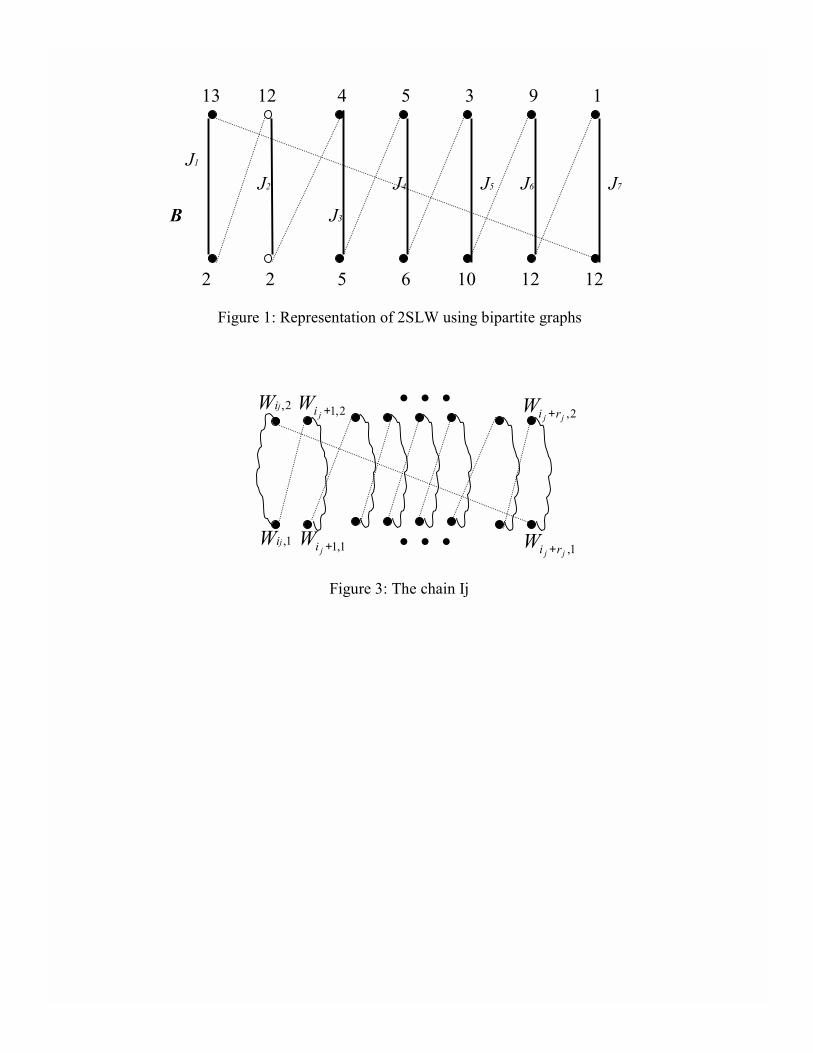
Example: Consider the 7-job problem with Wij given in Table 1. The bipartite graph B

corresponding to the sequence J1J2J3J4J5J6J7 is given in Figure 1. The dotted edges represent

the sequence matching I and the solid edges represent the job matching M .

Table 1: A 7-job example

i \ j 1 2

1 2 13

2 2 12

3 5 4

4 6 5

5 10 3

6 12 9

7 12 1

INSERT FIGURE 1 HERE

Evidently, for every permutation of the n jobs, the graph I∪M forms a Hamiltonian cycle; i.e.

a cycle that spans all the nodes of B. This Hamiltonian cycle consists of 2n edges that alternate

between the sets I and M . Since the job matching M is given, the matching I complements M

into a Hamiltonian cycle. For this reason, we refer to I ∪M as a complementary Hamiltonian

cycle or CHC. Let

wil =Wi1 +Wl2 for every edge (Wi1,Wl2) of B(V, U).

Then, 2SRW can be cast as a minimum cost CHC problem where cost is measured as the

difference between the largest and smallest edge costs wil among edges in I. Below we summarize

our observations.

Proposition 1 The sequence matching I corresponds to a permutation of the jobs in J if and

only if I ∪M is a complementary Hamiltonian cycle.

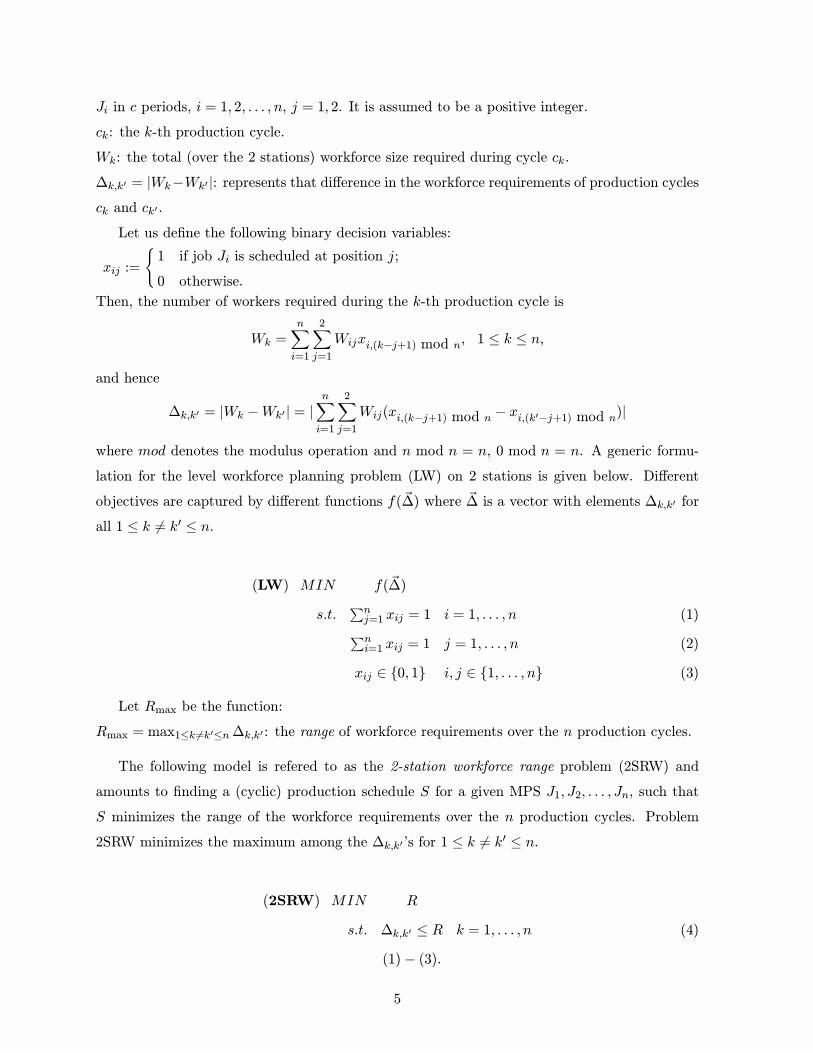
Example: Consider the CHC given in Figure 1. The workforce requirements for this cyclic

schedule for every production cycle are given in Table 2. Evidently, the total number of workers

required by this schedule is 21, the minimum number of workers required over all production

cycles is 3, and hence the range is R = ∆1,7 = 18.

The CHC representation for problem 2SRW extends naturally to problem 2SmW. The only

difference is that the matching I of an optimal CHC I ∪M should be such that the minimum

7

Table 2: An example schedule

Job\ Cycle 1 2 3 4 5 6 7

J1 2 13

J2 2 12

J3 5 4

J4 6 5

J5 10 3

J6 12 9

J7 1 12

Wk 3 15 17 10 15 15 21 Max = 21

Min = 3

edge cost wil is the largest possible. In what follows we develop solution algorithms for 2SmW

and 2SRW. We start our analysis with problem 2SmW because the algorithm developed for this

is used to obtain an optimal range schedule for 2SRW.

3 An Optimal Algorithm for 2SmW

In this section we develop an O(n log n) algorithm that solves the 2-station workforce problem

with the objective to maximize the minimum workforce requirement over the production horizon.

(2SmW) Wmin =MaxxMinkPni=1

P2j=1Wijxi,(k−j+1) mod n

s.t. (1)− (3.)

In the CHC representation of Section 2.1 for problem 2SmW, recall that matching I of an

optimal CHC I ∪ M should be such that the minimum edge cost wil is the largest possible.

Consider the relaxation of 2SmW where we want to Þnd an unconstrained perfect matching I

between the nodes of V and U so that the minimum edge cost is maximized. In other words, there

is no requirement that I ∪M forms a CHC. Then, the maximin edge cost of I is a lower bound

to the optimal solution of 2SmW. To present this result, let us redeÞne V = {vi : 1 ≤ i ≤ n}and U = {ui : 1 ≤ i ≤ n} so that

W11 ≤W21 . . . ≤Wn1, and W12 ≥W22 ≥ . . . ≥Wn2.

From now on we will refer to nodes in V ∪U by the associatedWij value. E.g., we use (Wi1,Wj2)

to denote edge (ui, vj) ∈ E(B). We can state the following result.

8

Lemma 1 Let Wmin be the optimal solution for 2SmW. Then,

Wmin ≤ min1≤i≤n{Wi1 +Wi2}.

Proof: Let IU be an unconstrained matching between the integers W11 ≤ W21 . . . ≤ Wn1 and

W12 ≥ W22 ≥ . . . ≥ Wn2. Let WU be the smallest cost among edges in IU . If Wmin is the

smallest edge cost of an optimal (and hence constrained) matching (i.e., assignment) for 2SmW,

we have Wmin ≤WU . To complete the proof it suffices to show that

WU = min1≤i≤n{Wi1 +Wi2}.

Indeed, consider two arbitrary pairs Wi1,Wj1 and Wk2,Wl2. Without loss of generality assume

thatWi1 ≤Wj1 andWk2 ≥Wl2. There are 2 possible matchings between these 2 pairs; matching

I1 = {(Wi1,Wk2), (Wj1,Wl2)} and matching I2 = {(Wi1,Wl2), (Wj1,Wk2)}. It is easy to verifythat

min{Wi1 +Wk2,Wj1 +Wl2} ≤ min{Wi1 +Wl2,Wj1 +Wk2}.

Hence, for any 2 arbitrary pairs, it is always optimal to order Wi1-values in nondecreasing order

and Wi2-values in nonincreasing order. Now, start with an arbitrary ordering of Wi1- and Wi2-

values, and apply this argument to every 4 values Wi1, Wj1, Wk2, and Wl2 that violate the

condition Wi1 ≤ Wj1 or Wk2 ≥ Wl2. After no more than¡n4

¢iterations, the Wi1�s will be in

nondecreasing order and the Wi2�s in nonincreasing order. Hence, WU = min1≤i≤n{Wi1+Wi2}.This completes the proof of the lemma. 2

Consider the unconstrained maximin matching

I0 = {(Wi1,Wi2) : 1 ≤ i ≤ n}

of Lemma 1. Generally, I0 ∪M is a union of subcycles that alternate between edges in I0 and

edges in M . In the event that I0 ∪M forms a CHC, we have Wmin = mini{Wi1 +Wi2}. LetC1, C2, . . . , Cr be the subcycles of I0 ∪M . The process of merging these subcycles into a CHCis known in the literature as patching and has been used extensively to solve variants of the

Traveling Salesperson problem; see Gilmore and Gomory, 1964, Karp, 1979 and Vairaktarakis

and Solow, 2001. A main result from this literature is described next.

Let G(C) be the graph with node set C = {C1, C2, . . . , Cr} and edge set

E(G) = {(Ci, Cj) : ∃ e = (Wk1,Wl2) ∈ B(V, U) s.t. Ci (Cj) traverses Wk1 (Wl2)}.

Then we can state the following known result.

9

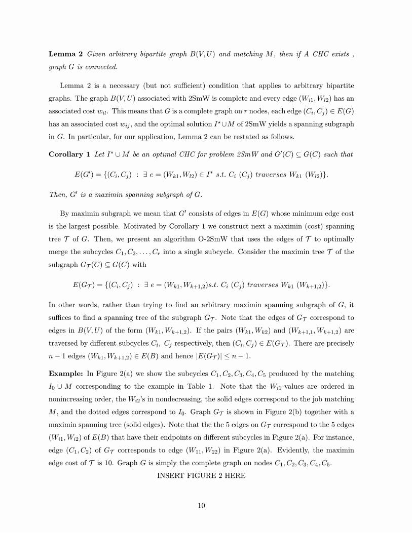
Lemma 2 Given arbitrary bipartite graph B(V, U) and matching M , then if A CHC exists ,

graph G is connected.

Lemma 2 is a necessary (but not sufficient) condition that applies to arbitrary bipartite

graphs. The graph B(V, U) associated with 2SmW is complete and every edge (Wi1,Wl2) has an

associated cost wil. This means that G is a complete graph on r nodes, each edge (Ci, Cj) ∈ E(G)has an associated cost wij , and the optimal solution I

?∪M of 2SmW yields a spanning subgraph

in G. In particular, for our application, Lemma 2 can be restated as follows.

Corollary 1 Let I∗ ∪M be an optimal CHC for problem 2SmW and G0(C) ⊆ G(C) such that

E(G0) = {(Ci, Cj) : ∃ e = (Wk1,Wl2) ∈ I∗ s.t. Ci (Cj) traverses Wk1 (Wl2)}.

Then, G0 is a maximin spanning subgraph of G.

By maximin subgraph we mean that G0 consists of edges in E(G) whose minimum edge cost

is the largest possible. Motivated by Corollary 1 we construct next a maximin (cost) spanning

tree T of G. Then, we present an algorithm O-2SmW that uses the edges of T to optimally

merge the subcycles C1, C2, . . . , Cr into a single subcycle. Consider the maximin tree T of the

subgraph GT (C) ⊆ G(C) with

E(GT ) = {(Ci, Cj) : ∃ e = (Wk1,Wk+1,2)s.t. Ci (Cj) traverses Wk1 (Wk+1,2)}.

In other words, rather than trying to Þnd an arbitrary maximin spanning subgraph of G, it

suffices to Þnd a spanning tree of the subgraph GT . Note that the edges of GT correspond to

edges in B(V, U) of the form (Wk1,Wk+1,2). If the pairs (Wk1,Wk2) and (Wk+1,1,Wk+1,2) are

traversed by different subcycles Ci, Cj respectively, then (Ci, Cj) ∈ E(GT ). There are preciselyn− 1 edges (Wk1,Wk+1,2) ∈ E(B) and hence |E(GT )| ≤ n− 1.

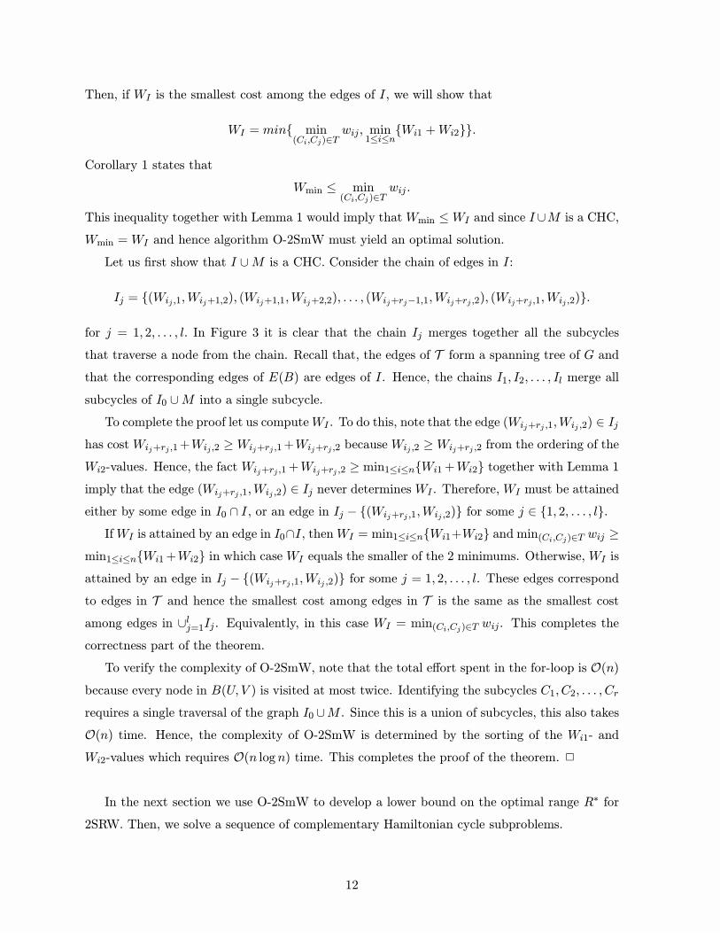
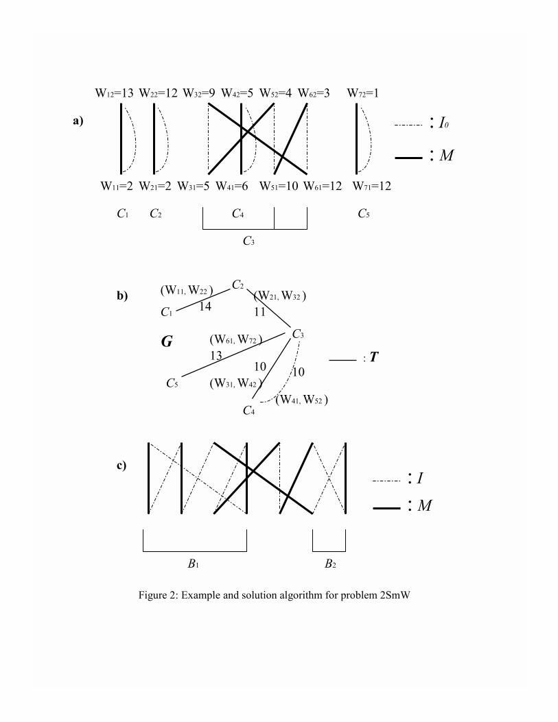
Example: In Figure 2(a) we show the subcycles C1, C2, C3, C4, C5 produced by the matching

I0 ∪ M corresponding to the example in Table 1. Note that the Wi1-values are ordered in

nonincreasing order, the Wi2�s in nondecreasing, the solid edges correspond to the job matching

M , and the dotted edges correspond to I0. Graph GT is shown in Figure 2(b) together with a

maximin spanning tree (solid edges). Note that the the 5 edges on GT correspond to the 5 edges

(Wi1,Wi2) of E(B) that have their endpoints on different subcycles in Figure 2(a). For instance,

edge (C1, C2) of GT corresponds to edge (W11,W22) in Figure 2(a). Evidently, the maximin

edge cost of T is 10. Graph G is simply the complete graph on nodes C1, C2, C3, C4, C5.

INSERT FIGURE 2 HERE

10

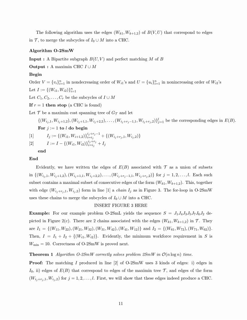
The following algorithm uses the edges (Wk1,Wk+1,2) of B(V,U) that correspond to edges

in T , to merge the subcycles of I0 ∪M into a CHC.

Algorithm O-2SmW

Input : A Bipartite subgraph B(U, V ) and perfect matching M of B

Output : A maximin CHC I ∪MBegin

Order V = {vi}ni=1 in nondecreasing order of Wi1�s and U = {ui}ni=1 in nonincreasing order of Wi2�s

Let I := {(Wi1,Wi2)}ni=1Let C1, C2, . . . , Cr be the subcycles of I ∪MIf r = 1 then stop (a CHC is found)

Let T be a maximin cost spanning tree of GT and let

{(Wij ,1,Wij+1,2), (Wij+1,1,Wij+2,2), . . . , (Wij+rj−1,1,Wij+rj ,2)}lj=1 be the corresponding edges in E(B).For j := 1 to l do begin

[1] Ij := {(Wi1,Wi+1,2)}ij+rj−1i=ij+ {(Wij+rj ,1,Wij ,2)}

[2] I := I − {(Wi1,Wi2)}ij+rji=ij+ Ij

end

End

Evidently, we have written the edges of E(B) associated with T as a union of subsets

in {(Wij ,1,Wij+1,2), (Wij+1,1,Wij+2,2), . . . , (Wij+rj−1,1,Wij+rj ,2)} for j = 1, 2, . . . , l. Each suchsubset contains a maximal subset of consecutive edges of the form (Wk1,Wk+1,2). This, together

with edge (Wij+rj ,1,Wij ,2) form in line [1] a chain Ij as in Figure 3. The for-loop in O-2SmW

uses these chains to merge the subcycles of I0 ∪M into a CHC.

INSERT FIGURE 3 HERE

Example: For our example problem O-2SmL yields the sequence S = J1J4J3J5J7J6J2 de-

picted in Figure 2(c). There are 2 chains associated with the edges (Wk1,Wk+1,2) in T . Theyare I1 = {(W11,W22), (W21,W32), (W31,W42), (W41,W12)} and I2 = {(W61,W72), (W71,W62)}.Then, I = I1 + I2 + {(Wi1,Wi2)}. Evidently, the minimum workforce requirement in S is

Wmin = 10. Correctness of O-2SmW is proved next.

Theorem 1 Algorithm O-2SmW correctly solves problem 2SmW in O(n log n) time.Proof: The matching I produced in line [2] of O-2SmW uses 3 kinds of edges: i) edges in

I0, ii) edges of E(B) that correspond to edges of the maximin tree T , and edges of the form(Wij+rj ,1,Wij ,2) for j = 1, 2, . . . , l. First, we will show that these edges indeed produce a CHC.

11

Then, if WI is the smallest cost among the edges of I, we will show that

WI = min{ min(Ci,Cj)∈T

wij, min1≤i≤n{Wi1 +Wi2}}.

Corollary 1 states that

Wmin ≤ min(Ci,Cj)∈T

wij .

This inequality together with Lemma 1 would imply that Wmin ≤WI and since I∪M is a CHC,

Wmin =WI and hence algorithm O-2SmW must yield an optimal solution.

Let us Þrst show that I ∪M is a CHC. Consider the chain of edges in I:

Ij = {(Wij ,1,Wij+1,2), (Wij+1,1,Wij+2,2), . . . , (Wij+rj−1,1,Wij+rj ,2), (Wij+rj ,1,Wij ,2)}.

for j = 1, 2, . . . , l. In Figure 3 it is clear that the chain Ij merges together all the subcycles

that traverse a node from the chain. Recall that, the edges of T form a spanning tree of G and

that the corresponding edges of E(B) are edges of I. Hence, the chains I1, I2, . . . , Il merge all

subcycles of I0 ∪M into a single subcycle.

To complete the proof let us computeWI . To do this, note that the edge (Wij+rj ,1,Wij ,2) ∈ Ijhas cost Wij+rj ,1+Wij ,2 ≥Wij+rj ,1+Wij+rj ,2 because Wij ,2 ≥Wij+rj ,2 from the ordering of the

Wi2-values. Hence, the fact Wij+rj ,1+Wij+rj ,2 ≥ min1≤i≤n{Wi1+Wi2} together with Lemma 1imply that the edge (Wij+rj ,1,Wij ,2) ∈ Ij never determines WI . Therefore, WI must be attained

either by some edge in I0 ∩ I , or an edge in Ij − {(Wij+rj ,1,Wij ,2)} for some j ∈ {1, 2, . . . , l}.IfWI is attained by an edge in I0∩I, thenWI = min1≤i≤n{Wi1+Wi2} and min(Ci,Cj)∈T wij ≥

min1≤i≤n{Wi1+Wi2} in which case WI equals the smaller of the 2 minimums. Otherwise, WI is

attained by an edge in Ij − {(Wij+rj ,1,Wij ,2)} for some j = 1, 2, . . . , l. These edges correspondto edges in T and hence the smallest cost among edges in T is the same as the smallest cost

among edges in ∪lj=1Ij . Equivalently, in this case WI = min(Ci,Cj)∈T wij. This completes the

correctness part of the theorem.

To verify the complexity of O-2SmW, note that the total effort spent in the for-loop is O(n)because every node in B(U, V ) is visited at most twice. Identifying the subcycles C1, C2, . . . , Cr

requires a single traversal of the graph I0 ∪M . Since this is a union of subcycles, this also takesO(n) time. Hence, the complexity of O-2SmW is determined by the sorting of the Wi1- and

Wi2-values which requires O(n log n) time. This completes the proof of the theorem. 2

In the next section we use O-2SmW to develop a lower bound on the optimal range R∗ for

2SRW. Then, we solve a sequence of complementary Hamiltonian cycle subproblems.

12

4 An Optimal Algorithm for Problem 2SRW

In this section we develop an efficient algorithm for 2SRW. The complexity of problem 2SRW

has been considered in Vairaktarakis and Cai, 2001.

Theorem 2 (Vairaktarakis and Cai, 2001)

Problem 2SRW is NP-complete in the strong sense.

In light of Theorem 2, the best way to address the problem is via enumerative methods.

Such methods are signiÞcantly expedited with the use of lower bounds. An efficient lower bound

is developed next.

4.1 A Lower Bound

As we saw in Section 2 problem 2SRW is equivalent to minxmax1≤k<k0≤n∆k,k0 subject to con-

straints (1)-(3). Let S? be an optimal schedule for 2SRW with range value R? equal to

R? =Wk0 −Wk00 for some 1 ≤ k0 6= k00 ≤ n.

Then, Wk0 , Wk00 are the largest and smallest number of workers respectively required by S? over

the n production cycles. Consider the subproblems 2SmW and

(2SMW) Wmax =MinxijMaxkPni=1

P2j=1Wijxi,(k−j+1) mod n

s.t. (1)− (3).

Problem 2SMW Þnds a schedule with the smallest possible value for the maximum workforce

size over all periods of the production horizon. Hence,

Wk0 ≥Wmax.

Problem 2SmW Þnds a schedule with the largest possible value for the minimum workforce size

over the production horizon. Hence,

W 0k0 ≤Wmin.

Combining these two inequalities we obtain the following lower bound.

Lemma 3

LB =Wmax −Wmin ≤ R∗.

An optimal algorithm 2SMW is presented in Lee and Vairaktarakis, 1997. The complexity of

2SMW is O(n log n). Algorithm O-2SmW requires O(n log n) time as well (Theorem 1). Hence,

this is also the time required to compute LB. The following theorem provides a range of values

for Wk0 and W0k0.

13

Theorem 3 Let R? =Wk0 −Wk00 for some 1 ≤ k0 6= k00 ≤ n Then,

Wmax ≤Wk0 ≤Wmin +R, and Wmax −R ≤Wk00 ≤Wmin,

where R = min{RM , Rm} and RM , Rm are the range values associated with the solutions obtainedby 2SMW and 2SmW respectively.

Proof: First we show Wmax ≤ Wk0 ≤ Wmin + R. We have already seen the left part of this

inequality. Since R? =Wk0−Wk00 we haveWk0 = R?+Wk00 . The solutions of 2SMW and 2SmW

are not necessarily optimal for 2SRW and hence R ≥ R?. Also, we have seen that Wk00 ≤Wmin.

Hence, Wk0 ≤ Wmin + R. Proving Wmax − R ≤ Wk00 ≤ Wmin is analogous. This completes the

proof of the theorem. 2

Example: As an example, consider the problem in Table 1. In Section 3 we saw that the optimal

sequence is Sm = J1J4J3J5J7J6J2 and Wmin = 10. The maximum worforce requirement for Sm

is 19 and hence Rm = 9. Applying the algorithm of Lee and Vairaktarakis for 2SMW on the

instance of Table 1 yields the sequence SM = J1J2J3J5J7J6J4 and Wmax = 17. The minimum

worforce requirement for SM is 7 and hence RM = 10. Therefore, R = min{9, 10} = 9 is an

upper bound on R∗. Then, according to Theorem 3, Wk0 ∈ [17, 19] and Wk00 ∈ [8, 10].

In the next subsection we use the ranges provided in Theorem 3 within a 2-dimensional

search framework to solve problem 2SRW optimally.

4.2 Solution Algorithm

One way to identify an optimal solution for 2SRW is the following. Associated to every edge

(Wi1,Wl2) in B(V, U) is the edge weight wil =Wi1+Wl2. For given bounds WU and WL for the

largest and smallest number of workers required over the n production cycles, let B(WL,WU )

be the restriction of B(V, U) on edges with costs wil such that

WL ≤ wil ≤WU .

Then, according to Proposition 1 there exists a solution for 2SRWwithWL ≤Wk ≤WU for every

k = 1, 2, . . . , n if and only if there exists a complementary Hamiltonian cycle for B(WL,WU ).

Iterating over all possible values for WU and WL can therefore produce an optimal solution for

2SRW.

Theorem 3 provides a tight range of values for each of Wk0, Wk00 . Using these ranges one can

employ a 2-dimensional search to compute the optimal range value R∗. For each pair of trial

values, say WU and WL, we can solve the CHC problem on the graph B(WL,WU ). The CHC

problem is shown to be strongly NP-complete; see Vairaktarakis and Solow, 2001. However,

14

using the algorithm of Vairaktarakis and Solow, 2001 we can solve problems of up to 250 jobs

in less than 1 second. Hence, a 2-dimensional search combined with the CHC algorithm is

computationally feasible. Depending on how the 2-dimensional search is designed, the resulting

computational requirements may be signiÞcantly different. We propose 2 alternative search

schemes.

In the Þrst scheme we let WL take on every integer value in [(Wmax − R)+,Wmin] where

x+ is the positive part of integer x. For every such WL we perform bisection search on the

range [Wmax,Wmin + R] to identify the smallest integer WU for which a CHC exists for the

subset of E(B) where WL ≤ wil ≤ WU for every edge (Wi1,Wl2). The number of integers in

[(Wmax−R)+,Wmin] and [Wmax,Wmin+R] is no more than 2maxil wil becauseWmax,Wmin, R ≤maxil wil. Hence, the complexity of this approach results to O(wmax logwmax) CHC subproblemswhere wmax = maxil wil. This approach does not depend on the number of jobs; just the

maximum number of workers over all operations. When the number of workers is relatively

small, the approach is expected to perform satisfactorily.

An alternative search that involves polynomially many CHC subproblems is the following.

Let Z1 < Z2 < . . . < Zr be the distinct wil values in the range [(Wmax − R)+,Wmin]. Also,

let Z 01 < Z 02 < . . . < Z 0s be the distinct wil values in the range [Wmax,Wmin + R]. Since

there are at most n2 wil-values (because wil =Wi1 +Wl2), we have r, s ≤ n2. For each Z-valueperform bisection search to identify the smallest Z 0-value for which the associated CHC problem

is feasible. This approach requires O(n2 log n) time and hence it is strongly polynomial. Forlarge values of n this approach is expected to be inefficient.

Example: As we saw, Theorem 3 implies that Wk0 ∈ [17, 19] and W 0k0∈ [8, 10] for our example.

Note that all integers in [17, 19] and [8, 10] are possibleWi1+Wl2 sums. Depending on our choice

of 2-dimensional search, different (WL,WU ) pairs are tested. In both cases, when Wk0 = 17 we

get that the optimalWk00 is 10 and hence R = 7. The sequence obtained is RS = J1J2J3J4J5J7J6.

This sequence requires no more than 17 workers, and no production cycle requires less than 10

workers. This is the best possible R-value over all combinations, so R∗ = 7. In this particular

example the optimal sequence accieves both Wmin and Wmax. In general, this is not possible.

Then, it is important to know how well the optimal range schedule performs with respect to the

maximin and minimax schedules, and vice-versa. This is done empirically in the next section.

5 Computational Experiments

In our computational experiments we tested the computational efficiency of O-2SRW and the

value of the resulting schedule as compared with those obtained by O-2SmW and O-2SMW.

15

The code for O-2SRW used the code for solving the CHC problem in bipartite graphs that

was used in Vairaktarakis and Solow, 2001. Algorithm O-2SMW was reproduced from Lee and

Vairaktarakis, 1997. All code was written in C++ and experiments where performed on a PC

running at 266 MHz. We considered problem sizes that are multiples of 50, up to n = 250 jobs.

Fifty problems were solved for each value of n. In all problems, the Wij-values were drawn

randomly from the discrete uniform distribution on [5, 30].

We measured the computational efficiency of O-2SmW and O-2SRW in CPU seconds. As

expected, algorithm O-2SmW yielded the optimal solution in negligible time for all problems

considered including those with 250 jobs. For this reason we do not report these times. The

CPU times reported in Table 3 are averages over the 50 problems tested for every value of n.

These times do not include the time required to Þnd Wmin and Wmax, however, as we mentioned

these times are negligible (less than one hundrendth of a second). Evidently, the CPU times for

O-2SRW are in the order of a few seconds and increase slowly with n. Hence, we deem O-2SRW

as very efficient.

Table 3: Comparative performance of workforce range and size

n CPU R(Wmax)−R∗R∗ × 100% Wmin−Wmin(R)

Wmin× 100% Wmax(R)−Wmax

Wmax× 100%

50 0.346 3.45 0.57 0.51

100 0.922 4.14 0.62 0.54

150 1.870 4.84 0.64 0.57

200 3.285 5.45 0.66 0.58

250 4.981 6.11 0.66 0.58

To evaluate the comparative performance of the schedules obtained by O-2SmW, O-2SMW

and O-2SRW against the objectives Wmin, Wmax and R, we deÞned the following 3 statistics.

Let

Wmin(R): the minimum workforce requirement of the schedule obtained by O-2SRW,

Wmax(R): the maximum workforce requirement of the schedule obtained by O-2SRW,

R(Wmax): the range value of the schedule obtained by O-2SMW.

We deÞne the following statistics.

R(Wmax)−R∗R∗ × 100%: the relative percentage difference of the range value associated with SM ,

from R∗.Wmin−Wmin(R)

Wmin× 100%: the relative percentage difference of the minimum workforce requirement

associated with SR, from Wmin.

16

Wmax(R)−Wmax

Wmax×100%: the relative percentage difference of the maximum workforce requirement

associated with SR, from Wmax.

These 3 statistics were computed for every problem. In Table 3 we report the average values

(per statistic) over the 50 problems tested for each n value. Let SM , Sm and SR be the optimal

schedules for objectives Wmax, Wmin and R. The Þrst statistic captures the range performance

of schedule SM . Evidently, it deteriorates linearly as n increases, and is in excess of 6% for

250 jobs. In other words, minimizing the number of workers needed to complete all jobs in a

2-station transfer line carries a 6% range premium over the optimal range schedule.

The second statistic captures the performance of SR with respect to the minimum workforce

requirement. As evidenced in Table 3, SR is within 0.7% of Wmin. Problem size does not seem

to affect this performance. These Þgures indicate that the range schedule is nearly optimal even

if it is evaluated against the Wmin objective. The third statistic is used to evaluate SR against

Wmax. Again, irrespective of problem size, SR is within 0.6% of the optimal workforce size.

Combining the last 2 observations we conclude that the range schedule is nearly optimal for the

other 2 objectives.

The main insight from the above observations is that, using the optimal range schedule not

only minimizes workforce size disruptions across cycles, but also achieves this performance with

a minimal increase in workforce size. Cast differently, a 0.5% increase in workforce can protect

a transfer assembly line from unnecessary disruptions in the size of the workforce from one day

to the next.

6 Conclusion

In this article we developed tools for the range and maximin workforce leveling objectives for

2-station transfer lines. We used these tools to develop insights on the relative value of the

various schedules. Our study is conÞned to 2 stations for methodological reasons. For three

or more stations, the graph theoretic representation does not extend to an easily manageable

construct. Theorem 3 still holds but problems 3SMW and 3SmW are already strongly NP-

complete subproblems. Hence, integer programming approaches seem to be the likely candidate

for more than 2 stations. Completely different approaches are needed. Our future research

in this area will focus on such approaches. The observations made in this article on the near

optimality of range schedules when evaluated on workforce size, are expected to be even more

pronounced for more than 2 stations. Intuitively, the larger the number of stations, the greater

the contribution of individual stations to the range. Hence, a schedule that does not optimize

the range may have a horrible range performance. These observations indicate the need for

17

further research. Consideration of objective functions other than R and Wmin is also desirable.

References[1] Bartholdi J.J. III (1992). Balancing 2-Sided Assembly Lines (A Case Study). Working

Paper.

[2] Bartholdi J.J. III, D.D. Eisenstein (1996). A Production Line That Balances Itself. Oper-ations Research 44(1):21-34.

[3] Chen F.F. and E.E. Adam, Jr. (1991). The Impact of Flexible Manufacturing Systems onProductivity and Quality. IEEE Transactions on Engineering Management 38:33-45.

[4] Daniels R.L. and J.B. Mazzola (1993). A Tabu-Search Heuristic for the Flexible-ResourceFlow Shop Scheduling Problem. Management Science 41:207-230.

[5] Daniels R.L., B.J. Hoopes and J.B. Mazzola (1997). An Analysis of Heuristics for theParallel-Machine Flexible-Resource Scheduling Problem. Annals of Operations Research70:439-472.

[6] Ebeling A.C. and C.-Y. Lee (1993). Cross-training effectiveness and proÞtability. To appearin International Journal of Production Research.

[7] Fry T.D., M.G. Wilson and M. Breen (1987). A Successful Implementation of GroupTechnology and Cell Manufacturing. Production and Inventory Management 28:4-6.

[8] Goodrich T.H. (1988). Just-in-Time with an Emphasis on Group Technology. Manufac-turing Systems 6:78-79.

[9] Gilmore P. C. and R. E. Gomory. Sequencing a One State-Variable Machine: A SolvableCase of the Traveling Salesman Problem, Operations Research, 12:655-679, 1964.

[10] Hyer N.L. (1984). The Potential of Group Technology for U.S. Manufacturing. Journal ofOperations Management 4:183-202.

[11] Karp R.M. A Patching Algorithm for the Nonsymmetric Traveling Salesman Problem,SIAM Journal on Computing, 8:561-573. 1979.

[12] Lee C.-Y. and G. Vairaktarakis. Workforce Planning in Mixed Model Transfer Lines, Op-erations Research, 45(4):553-567, 1997.

[13] Pinto P.A., D.G. Dannenbring and B.M. Khumawala (1981). Branch and Bound andHeuristic Procedures for Assembly Line Balancing With Parallel Stations. InternationalJournal of Production Research 19:565-576.

[14] Vairaktarakis G. and X.Q. Cai. Complexity of Workforce Scheduling in Transfer Lines,Journal of Global Optimization, submitted, 2001.

[15] Vairaktarakis G., X.Q. Cai and C-Y Lee. Workforce Planning in Synchronous ProductionSystems, European Journal of Operations Research, Forthcoming, 2001.

[16] Vairaktarakis G and D. Solow. Properties of Complementary Hamiltonian Cycles on Bi-partite Graphs, Weatherhead School of Management, Dept. of Operations, Case WesternReserve University, Research Report, 2001.

[17] Vairaktarakis G and D. Solow. An Efficient Algorithm for the Complementary HamiltonianCycle Problem on Bipartite Graphs, INFORMS Journal on Computing, submitted, 2001.

18

[18] Vollmann, T.E, Berry, W.L. and Whybark, D.C, Manufacturing Planning and ControlSystems. Irwin/MGraw-Hill, U.S.A., 1997.

19

2

B

13

2

12

5 6

4 5

10

3

J1J2

J3

J4 J5

Figure 1: Representation of 2SLW using bipartite graphs

12

9

12

1

J6 J7

Figure 3: The chain Ij

2,jiW 2,1+jiW 2,jj riW +

�

1,jiW 1,1+jiW 1,jj riW +

�

W12=13 W22=12 W32=9 W42=5 W52=4 W62=3 W72=1

W11=2 W21=2 W31=5 W41=6 W51=10 W61=12 W71=12

C1 C2 C4 C5

C3

a)

C1

C2

C4

C5

C3

14 11

101013 : T

b)

B1 B2

c)

Figure 2: Example and solution algorithm for problem 2SmW

: I0: M

G

: I: M

(W11, W22 ) (W21, W32 )

(W31, W42 )(W41, W52 )

(W61, W72 )