12/1/2015 Gerris tutorial http://gfs.sourceforge.net/tutorial/tutorial/tutorial1.html 1/20 The Gerris Tutorial Version 1.3.2 Stéphane Popinet [email protected]March 23, 2011 Contents 1 Introduction 1.1 Simulation file 2 A simple simulation file 2.1 A few comments on syntax 2.2 Topology description of the simulation domain 2.3 Controlling the simulation 2.3.1 Spatial discretisation 2.3.2 Initial conditions 2.3.3 Writing results 3 A more complex example with solid boundaries 3.1 Domain geometry and boundary conditions 3.1.1 Boundary conditions 3.1.2 Solid boundaries 3.2 Saving the whole simulation 3.3 Visualisation 3.3.1 GfsView 3.3.2 Some postprocessing using gfs2oogl 3.4 Using dynamic adaptive mesh refinement 4 Going further 4.1 More on boundary conditions 4.2 Adding tracers 4.3 Adding diffusion terms 4.3.1 Boundary conditions for diffusion terms 4.4 Outputs 4.5 Boundary conditions 5 Running Gerris in parallel 6 Learning more 7 Do you want to help? 1 Introduction This tutorial is a stepbystep introduction to the different concepts necessary to use Gerris. It is specifically designed for a enduser and is not a technical description of the numerical techniques used within Gerris. If you are interested by that, you should consult the bibliography section on the Gerris web site. Various versions of this tutorial are available: Printable format: PDF. HTML: direct link or compressed archive. In this tutorial I will assume that you are familiar with the Unix shell (and that you are running some version of a Unix system). Some knowledge of C programming would also be very helpful if you intend to extend Gerris with your own objects. If Gerris is not already installed on your system, have a look at the installation instructions on the Gerris web site. We are now ready to start. Just to check that everything is okay try: % gerris2D ‐V
3 A more complex example with solid boundaries3.1 Domain geometry and boundary conditions
3.1.1 Boundary conditions3.1.2 Solid boundaries
3.2 Saving the whole simulation3.3 Visualisation
3.3.1 GfsView3.3.2 Some postprocessing using gfs2oogl
3.4 Using dynamic adaptive mesh refinement4 Going further
4.1 More on boundary conditions4.2 Adding tracers4.3 Adding diffusion terms
4.3.1 Boundary conditions for diffusion terms4.4 Outputs4.5 Boundary conditions
5 Running Gerris in parallel6 Learning more7 Do you want to help?
1 Introduction
This tutorial is a stepbystep introduction to the different concepts necessary to use Gerris. It is specifically designed fora enduser and is not a technical description of the numerical techniques used within Gerris. If you are interested by that,you should consult the bibliography section on the Gerris web site.
Various versions of this tutorial are available:
Printable format: PDF.HTML: direct link or compressed archive.
In this tutorial I will assume that you are familiar with the Unix shell (and that you are running some version of a Unixsystem). Some knowledge of C programming would also be very helpful if you intend to extend Gerris with your ownobjects.
If Gerris is not already installed on your system, have a look at the installation instructions on the Gerris web site.
We are now ready to start. Just to check that everything is okay try:
Gerris is a consolebased program. It takes a parameter or simulation file as input and produces various types of files asoutput. Everything needed to run the simulation is specified in the parameter file, this includes:
Layout of the simulation domainInitial conditionsBoundary conditionsSolid boundariesWhat to output (and when)Control parameters for the numerical schemes
2 A simple simulation file
In this section we will see how to write a simulation file for the initial random vorticity example in the Gerris web sitegallery. First of all, it is always a good idea to run simulations in their own directory. Type this at your shell prompt:
% mkdir vorticity% cd vorticity
As a starting point we will use the following simulation file: vorticity.gfs
1 2 GfsSimulation GfsBox GfsGEdge GfsTime end = 0 GfsBox 1 1 right1 1 top
This is a valid simulation file but it does not do much as you can see by typing
% gerris2D vorticity.gfs
It is a good starting point however to explain the general structure of a simulation file.
2.1 A few comments on syntax
First of all, there are two types of parameters in a simulation file: compulsory and optional parameters. Optionalparameters are always specified within a braced block (i.e. a block of text delimited by braces ( like this ). Theyalso often take the form
parameter = value
where parameter is an unique identifier (within this braced block). All the other parameters are compulsory parameters.For example, in vorticity.gfs both
GfsTime end = 0
and
end = 0
are optional parameters.
The second important syntax point regards the way various fields are delimited. Newline (or “carriage return”) charactersare generally used to delimitate different “objects” in the simulation file. The only case where this rule does not apply iswithin braced blocks defining optional arguments of the form
For example, in vorticity.gfs the following blocks of text are all objects:
1 2 GfsSimulation GfsBox GfsGEdge GfsTime end = 0
GfsTime end = 0
GfsBox
1 1 right
1 1 top
Following this rule, vorticty.gfs could have been written equivalently as:
1 2 GfsSimulation GfsBox GfsGEdge GfsTime end = 0 GfsBox 1 1 right1 1 top
2.2 Topology description of the simulation domain
Ok, so what are all these “objects” for? The first line of the simulation file defines a graph representing the general layoutof the simulation domain and follows this syntax:
1st fieldnumber of nodes in the graph (1)
2nd fieldnumber of edges connecting the nodes (2)
3rd fieldobject type for the graph (GfsSimulation)
4th fielddefault object type for the nodes (GfsBox)
5th fieldobject type for the edges (GfsGEdge)
6th field1st optional parameters (braced block)
7th field2nd optional parameters (braced block)
We then jump to the end of the 2nd optional parameters to line
GfsBox
which describes the first (and unique in this case) node of the graph. The first field is the object type of the node(GfsBox), the second field contains optional parameters. The following two lines
3rd fieldspatial direction in which the two nodes are connected (right and top)
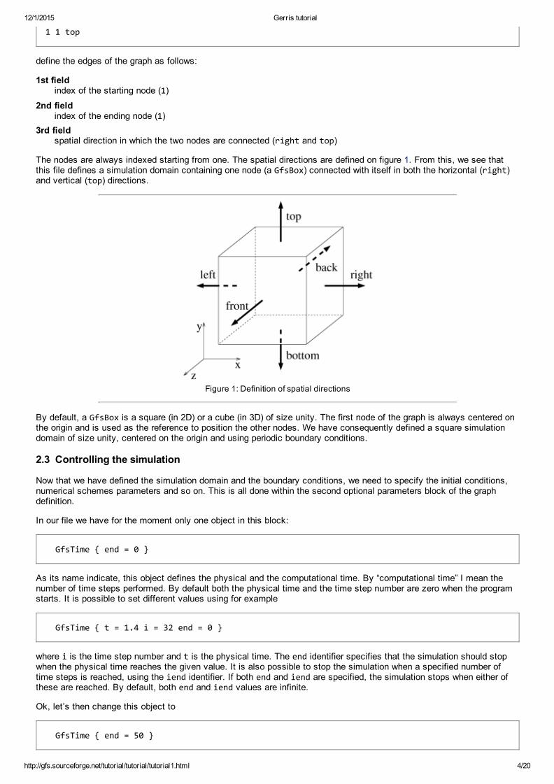
The nodes are always indexed starting from one. The spatial directions are defined on figure 1. From this, we see thatthis file defines a simulation domain containing one node (a GfsBox) connected with itself in both the horizontal (right)and vertical (top) directions.
Figure 1: Definition of spatial directions
By default, a GfsBox is a square (in 2D) or a cube (in 3D) of size unity. The first node of the graph is always centered onthe origin and is used as the reference to position the other nodes. We have consequently defined a square simulationdomain of size unity, centered on the origin and using periodic boundary conditions.
2.3 Controlling the simulation
Now that we have defined the simulation domain and the boundary conditions, we need to specify the initial conditions,numerical schemes parameters and so on. This is all done within the second optional parameters block of the graphdefinition.
In our file we have for the moment only one object in this block:
GfsTime end = 0
As its name indicate, this object defines the physical and the computational time. By “computational time” I mean thenumber of time steps performed. By default both the physical time and the time step number are zero when the programstarts. It is possible to set different values using for example
GfsTime t = 1.4 i = 32 end = 0
where i is the time step number and t is the physical time. The end identifier specifies that the simulation should stopwhen the physical time reaches the given value. It is also possible to stop the simulation when a specified number oftime steps is reached, using the iend identifier. If both end and iend are specified, the simulation stops when either ofthese are reached. By default, both end and iend values are infinite.
The next step is to specify what spatial resolution we want for the discretisation. For the moment, the only thing we havedefined is the root of the quad/octree. The whole domain is thus discretised with only one grid point…
We need to specify how we want to refine this initial root cell. This is done by using an GfsRefine object. We can do thisby adding the line
GfsRefine 6
to the second optional parameter block. This is the simplest possible way to refine the initial root cell. We tell the programthat we want to keep refining the cell tree (by dividing each cell in four children cells (in 2D, eight in 3D)) until the level ofthe cell is equal to five. The level of the root cell is zero, the level of all its children cells is one and so on recursively.After this refinement process completes we have created a regular Cartesian grid with 26=64 cells in each dimension onthe finest level (6).
2.3.2 Initial conditions
We now need to specify the initial conditions and the various actions (such as writing results, information messagesetc…) we want to perform when the simulation is running. All these things are treated by Gerris as various types ofevents, all represented by objects derived from the same parent object GfsEvent.
Initial conditions are a particular type of event happening only once and before any other type of event, they are allderived from the same parent object GfsInit.
Gerris comes with a few different objects describing various initial conditions. As there is no way Gerris could provide allthe different initial conditions users could think of, Gerris makes it easy for users to create their own initialisation objectsby extending the GfsInit object class. In order not to have to recompile (or more exactly relink) the whole codeeverytime a new class is added, Gerris uses dynamically linked modules which can be loaded at runtime. We will seelater how to write your own modules.
For the moment, we will use the default GfsInit object. Just add the following lines to vorticity.gfs:
1 2 GfsSimulation GfsBox GfsGEdge GfsTime end = 50 GfsRefine 6 GfsInit U = (0.5 ‐ rand()/(double)RAND_MAX) V = (0.5 ‐ rand()/(double)RAND_MAX) GfsBox 1 1 right1 1 top
Using GfsInit it is possible to set the initial value of each of the simulation variables. By default all variables are set tozero initially. In our case we tell Gerris to define the two components of the velocity field U and V as C functions. Thestandard rand function of the C library returns a (pseudo)random number between 0 and RAND_MAX. The two functionswe defined thus set the components of the velocities in each cell as random numbers between 0.5 and 0.5.
This is a powerful feature of the parameter file. In most cases where Gerris requires a number (such as the GfsRefine 6line, a function of space and time can be used instead. For example, a valid parameter file could include:
... GfsRefine 6.*(1. ‐ sqrt (x*x + y*y))...
which would define a mesh refined in concentric circles.
Using this feature, it is possible to define most initial conditions directly in the parameter file.
2.3.3 Writing results
The vorticity.gfs file we have now is all Gerris needs to run the simulation. However, for this run to be any use, weneed to specify how and when to output the results. This is done by using another class of objects: GfsOutput, derived
starting whenever the physical time is larger than (or equal to) 0.5 or the time step number is larger than (or equalto) 10,ending whenever the physical time is strictly larger than 3.4 or the time step number is strictly larger than 46,
and occurring every 10−2 physical time units.
It is also possible to specify an event step as a number of time steps using the istep identifier. Note, however, that youcannot specify both step and istep for the same event. By default, start and istart are zero and end, iend, stepand istep are infinite.
An GfsOutput object is derived from GfsEvent and follows this syntax:
GfsOutput filename‐%d‐%f‐%ld
The first part of the line GfsOutput defines the GfsEvent part of GfsOutput and follows the syntax above. In theremainder of this tutorial, I will use the following notation to express this inheritance of syntax:
[GfsEvent] filename‐%d‐%f‐%ld
to avoid repeating the whole thing for every derived objects.
The second part filename‐%d‐%f‐%ld specifies where to output things. The %d, %f and %ld characters are formattingstrings which follow the C language syntax and will be replaced every time the event takes place according to:
%dinteger replaced with the current process number (used when running the parallel version of Gerris).
%ffloatingpoint number replaced with the current physical time.
%ld(long) integer replaced with the current time step number.
Of course, you are free not to specify any of these, in which case the output will just be appended to the same file everytime the event takes place. There are also two filenames which have a special meaning: stdout and stderr, for thestandard output and standard error of the shell respectively.
We now add the following to our simulation file:
1 2 GfsSimulation GfsBox GfsGEdge GfsTime end = 50 GfsRefine 6 GfsInit U = (0.5 ‐ rand()/(double)RAND_MAX) V = (0.5 ‐ rand()/(double)RAND_MAX) GfsOutputTime istep = 10 stdout GfsOutputProjectionStats istep = 10 stdoutGfsBox 1 1 right1 1 top
The first line we added tells the program to output information about the time every 10 time steps on the standard output.The second line outputs statistics about the projection part of the algorithm.
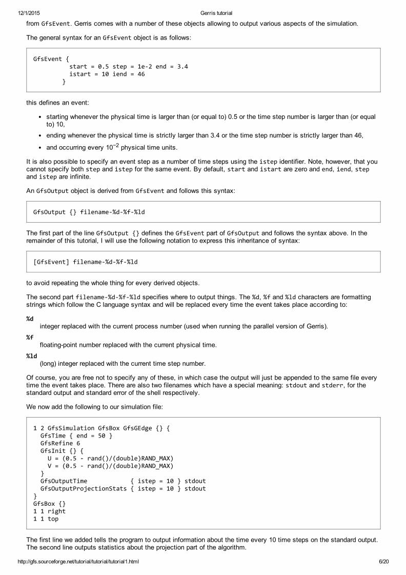
The lines starting with step: are written by GfsOutputTime. They give the time step number, corresponding physicaltime and the time step used for the previous iteration.
The other lines are written by GfsOutputProjectionStats and give you an idea of the divergence errors andconvergence rate of the two projection steps (MAC and approximate) performed during the previous iteration. The variousnorms of the residual of the solution of the Poisson equation are given before and after the projection step. The ratecolumn gives the average amount by which the divergence is reduced by each iteration of the multigrid solver.
Well, numbers are great but what about some images? What we want to do, for example, is output some graphicalrepresentation of a given scalar field. In 2D, a simple way to do that is to create an image where each pixel is colouredaccording to the local value of the scalar. Gerris provides an object to do just that: GfsOutputPPM which will create aPPM (Portable PixMap) image. This object is derived from a more general class used to deal with scalar fields:GfsOutputScalar following this syntax:
[GfsOutput] v = U min = ‐1 max = 2.5
where as before the square brackets express inheritance from the parent class. The v identifier specifies what scalar fieldwe are dealing with, one of:
U, V (and W in 3D): components of the velocity.
P: pressure.
C: passive tracer.
Vorticity: vorticity (norm of the vorticity vector in 3D).
The min and max values specify the minimum and maximum values this scalar can take. If they are not given, they arecomputed every time the event takes place.
We can now use this in our simulation file:
1 2 GfsSimulation GfsBox GfsGEdge GfsTime end = 50 GfsRefine 6 GfsInit U = (0.5 ‐ rand()/(double)RAND_MAX) V = (0.5 ‐ rand()/(double)RAND_MAX) GfsOutputTime istep = 10 stdout GfsOutputProjectionStats istep = 10 stdout GfsOutputPPM step = 1 vorticity‐%4.1f.ppm v = Vorticity GfsBox 1 1 right1 1 top
The code will output every 1 time units a PPM image representing the vorticity field. The result will be written in filesnamed: vorticity‐00.0.ppm, vorticity‐01.0.ppm…(if the %4.1f thing is not familiar, consult a C book or try % man3 printf).
If you rerun the program using this new simulation file, you will get a number of PPM files (51 to be precise) you canthen visualise with any image editing or viewing tool. I would recommend the very good ImageMagick toolbox. If you runa Linux box, these tools are very likely to be already installed on your system. Try typing this in your working directory:
% display *.ppm
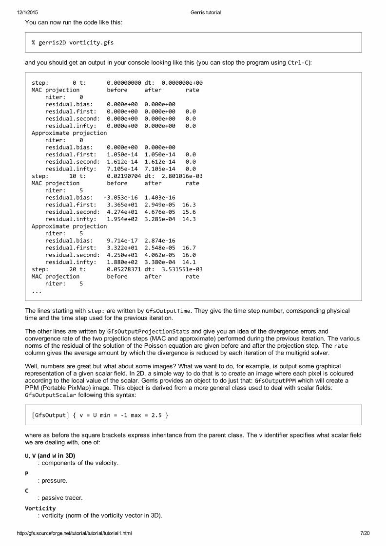
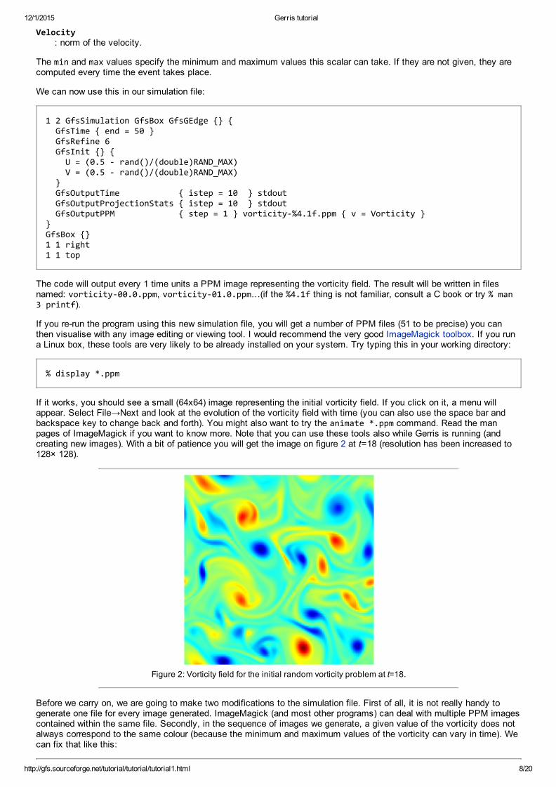
If it works, you should see a small (64x64) image representing the initial vorticity field. If you click on it, a menu willappear. Select File→Next and look at the evolution of the vorticity field with time (you can also use the space bar andbackspace key to change back and forth). You might also want to try the animate *.ppm command. Read the manpages of ImageMagick if you want to know more. Note that you can use these tools also while Gerris is running (andcreating new images). With a bit of patience you will get the image on figure 2 at t=18 (resolution has been increased to128× 128).
Figure 2: Vorticity field for the initial random vorticity problem at t=18.
Before we carry on, we are going to make two modifications to the simulation file. First of all, it is not really handy togenerate one file for every image generated. ImageMagick (and most other programs) can deal with multiple PPM imagescontained within the same file. Secondly, in the sequence of images we generate, a given value of the vorticity does notalways correspond to the same colour (because the minimum and maximum values of the vorticity can vary in time). Wecan fix that like this:
1 2 GfsSimulation GfsBox GfsGEdge GfsTime end = 50 GfsRefine 6 GfsInit U = (0.5 ‐ rand()/(double)RAND_MAX) V = (0.5 ‐ rand()/(double)RAND_MAX) GfsOutputTime istep = 10 stdout GfsOutputProjectionStats istep = 10 stdout GfsOutputScalarStats istep = 10 stdout v = Vorticity GfsOutputPPM step = 0.1 vorticity.ppm v = Vorticity min = ‐10 max = 10 GfsBox 1 1 right1 1 top
We have now specified fixed bounds for the vorticity (using the min and max identifiers). Each PPM image will beappended to the same file: vorticity.ppm.
How did I choose the minimum and maximum values for the vorticity? The line GfsOutputScalarStats istep = 10 stdout v = Vorticity , writes the minimum, average, standard deviation and maximum values of the vorticity.By rerunning the simulation and looking at these values it is easy to find a suitable range.
3 A more complex example with solid boundaries
In this section we will see how to set up a simulation for the flow past a solid body (a halfcylinder) in a narrow channel.While doing that we will also encounter new ways of displaying simulation results.
3.1 Domain geometry and boundary conditions
What we want is a narrow channel (4× 1 for example). From the previous example, we know that we can build it like this:
4 3 GfsSimulation GfsBox GfsGEdge GfsTime end = 0 GfsBox GfsBox GfsBox GfsBox 1 2 right2 3 right3 4 right
i.e. four boxes, box 1 connected to box 2 horizontally (to the right), box 2 connected to box 3 horizontally and box 3connected to box 4 horizontally. Box 1 is centered on the origin and is of size one. All the other boxes are positionedaccordingly. We now have our 4× 1 rectangular domain.
3.1.1 Boundary conditions
What about boundary conditions? By default Gerris assumes that boundaries are solid walls with slip conditions for thevelocity (i.e. the tangential stress on the wall is zero). For the moment we then have defined a rectangular box closed onall sides by solid walls.
What we really want is to specify an input velocity on the left side of the box and some sort of output condition on theright side. We can do that like this:
4 3 GfsSimulation GfsBox GfsGEdge GfsTime end = 0 GfsBox left = GfsBoundaryInflowConstant 1 GfsBox GfsBox
GfsBox right = GfsBoundaryOutflow 1 2 right2 3 right3 4 right
The whole left side of the first (leftmost) box is now defined to be a GfsBoundaryInflowConstant object and the wholeright side of the last (rightmost) box a GfsBoundaryOutflow object. Again, boundary conditions objects are all derivedfrom the GfsBoundary object and, as initial conditions, new objects can be easily written by the user (see also section4.1).
We see that GfsBoundaryInflowConstant takes one argument which is the value of the (constant) normal velocityapplied to this boundary. All the other variables (pressure, tracer concentration etc...) follow a zero gradient condition.
GfsBoundaryOutflow implements a simple outflow boundary condition where the pressure is set to zero as well as thegradient of all other quantities.
3.1.2 Solid boundaries
We now have an empty “wind tunnel” with a constant inlet velocity of norm unity. Gerris can deal with arbitrarily complexsolid boundaries embedded in the quad/octree mesh. The geometry of the solid boundaries is described using GTStriangulated surfaces. In 2D, using 3D triangulated surfaces seems overkill, as 2D curves would be enough. However,Gerris being both a 2D and 3D code it deals with 2D solid boundaries exactly as with 3D ones, even if the simulation isdone only on a 2D crosssection.
Creating 3D polygonal surfaces is not an easy job and is clearly outside the scope of this tutorial. There are a number ofutilities you can use to do that, including big commercial CAD packages. In general, once you have created a polygonalsurface with one of these tools it should be relatively easy to convert it to the file format used by GTS. In particular, mostCAD packages can export to the STL (stereolithography) format which is easily converted to the GTS file format usingthe stl2gts utility which comes with the library.
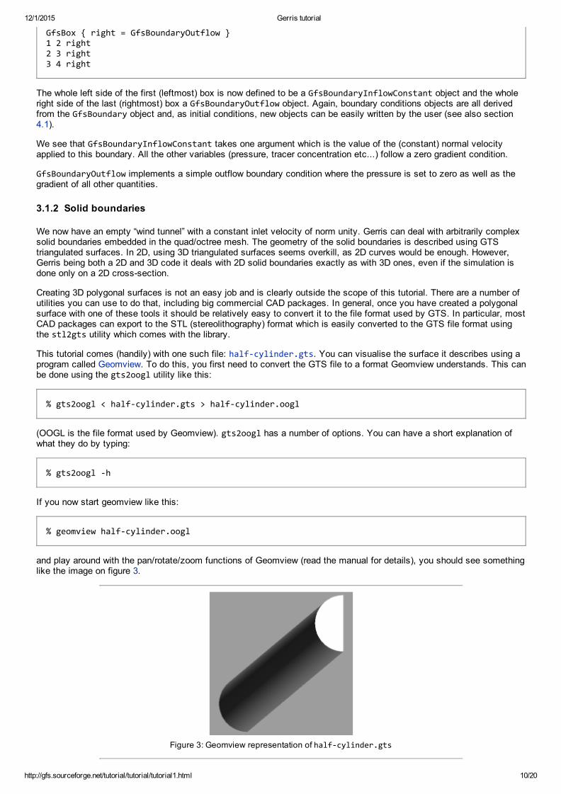
This tutorial comes (handily) with one such file: half‐cylinder.gts. You can visualise the surface it describes using aprogram called Geomview. To do this, you first need to convert the GTS file to a format Geomview understands. This canbe done using the gts2oogl utility like this:
You can notice that this is a proper 3D object, even if we are only going to simulate the flow in a 2D crosssection. It isalso important that the object is “tall” enough so that it spans the entire “height” of the 2D domain, as if we were going tosimulate the flow around it in a proper 3D channel with a square crosssection. The orientation of the surface is alsoimportant to define what is inside (the solid) and what is outside (the fluid).
We can now insert this object in the simulation domain like this:
4 3 GfsSimulation GfsBox GfsGEdge GfsTime end = 0 GfsSolid half‐cylinder.gtsGfsBox left = GfsBoundaryInflowConstant 1 GfsBox GfsBox GfsBox right = GfsBoundaryOutflow 1 2 right2 3 right3 4 right
add what mesh refinement we want and a few things to output:
4 3 GfsSimulation GfsBox GfsGEdge GfsTime end = 9 GfsRefine 6 GfsSolid half‐cylinder.gts GfsInit U = 1 GfsOutputBoundaries boundaries GfsOutputTime step = 0.02 stdout GfsOutputProjectionStats step = 0.02 stdout GfsOutputPPM step = 0.02 vorticity.ppm min = ‐100 max = 100 v = Vorticity GfsOutputTiming start = end stdoutGfsBox left = GfsBoundaryInflowConstant 1 GfsBox GfsBox GfsBox right = GfsBoundaryOutflow 1 2 right2 3 right3 4 right
I have added a new GfsOutput object we haven’t seen yet: GfsOutputTiming. This object writes a summary of the timetaken by various parts of the solver. You might also have noticed the unusual start = end bit ; this just specifies thatthis event will only happen once at the end of the simulation.
Another new output object is GfsOutputBoundaries. This object writes a geometrical summary (in OOGL/Geomviewformat) of the mesh used, including boundary conditions, solid boundaries and so on.
We also initialise the velocity field on the whole domain to a constant value (1,0,0). We could have left the velocity fieldto its default value of (0,0,0) but, given that we impose inflow boundary conditions, it would have meant that the initialvelocity would have been strongly divergent. Gerris always starts a simulation by a projection step (to fix problems likethis) but it is always a good idea to start with the best possible velocity field.
We can now run the code:
% gerris2D half‐cylinder.gfs
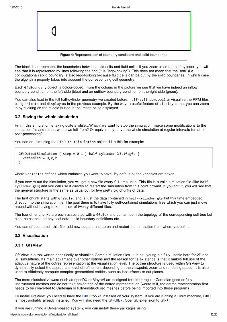
It is going to take a while to complete, but remember that you can look at files while they are being generated. The firstfile which will be generated is boundaries. If you load it in Geomview, you should get something like figure 4 (youprobably want to disable automatic normalization in Geomview by selecting Inspect→Appearance→Normalize→None).
Figure 4: Representation of boundary conditions and solid boundaries
The black lines represent the boundaries between solid cells and fluid cells. If you zoom in on the halfcylinder, you willsee that it is represented by lines following the grid (it is “legolooking”). This does not mean that the “real” (i.e.computational) solid boundary is also legolooking because fluid cells can be cut by the solid boundaries, in which casethe algorithm properly takes into account the corresponding cell geometry.
Each GfsBoundary object is colourcoded. From the colours in the picture we see that we have indeed an inflowboundary condition on the left side (blue) and an outflow boundary condition on the right side (green).
You can also load in the full halfcylinder geometry we created before: half‐cylinder.oogl or visualise the PPM filesusing animate and display as in the previous example. By the way, a useful feature of display is that you can zoomin by clicking on the middle button in the image being displayed.
3.2 Saving the whole simulation
Hmm, this simulation is taking quite a while…What if we want to stop the simulation, make some modifications to thesimulation file and restart where we left from? Or equivalently, save the whole simulation at regular intervals for latterpostprocessing?
You can do this using the GfsOutputSimulation object. Like this for example:
where variables defines which variables you want to save. By default all the variables are saved.
If you now rerun the simulation, you will get a new file every 0.1 time units. This file is a valid simulation file (like half‐cylinder.gfs) and you can use it directly to restart the simulation from this point onward. If you edit it, you will see thatthe general structure is the same as usual but for five pretty big chunks of data.
The first chunk starts with GfsSolid and is just the data contained in half‐cylinder.gts but this time embeddeddirectly into the simulation file. The goal there is to have fully selfcontained simulations files which you can just movearound without having to keep track of twenty different files.
The four other chunks are each associated with a GfsBox and contain both the topology of the corresponding cell tree butalso the associated physical data, solid boundary definitions etc...
You can of course edit this file, add new outputs and so on and restart the simulation from where you left it.
3.3 Visualisation
3.3.1 GfsView
GfsView is a tool written specifically to visualise Gerris simulation files. It is still young but fully usable both for 2D and3D simulations. Its main advantage over other options and the reason for its existence is that it makes full use of theadaptive nature of the octree representation at the visualisation level. The octree structure is used within GfsView todynamically select the appropriate level of refinement depending on the viewpoint, zoom and rendering speed. It is alsoused to efficiently compute complex geometrical entities such as isosurfaces or cutplanes.
The more classical viewers such as openDX or MayaVi are designed for either regular Cartesian grids or fullyunstructured meshes and do not take advantage of the octree representation (worse still, the octree representation firstneeds to be converted to Cartesian or fullyunstructured meshes before being imported into these programs).
To install GfsView, you need to have the Gtk+ toolkit installed on your system. If you are running a Linux machine, Gtk+is most probably already installed. You will also need the GtkGlExt OpenGL extension to Gtk+.
If you are running a Debianbased system, you can install these packages using
If you then download a recent version of GfsView from the Gerris web site (either an official release or a snapshot) and dothe now classical:
% gunzip gfsview.tar.gz% tar xvf gfsview.tar% cd gfsview% ./configure ‐‐prefix=/home/joe/local% make% make install
you will be able to start GfsView using:
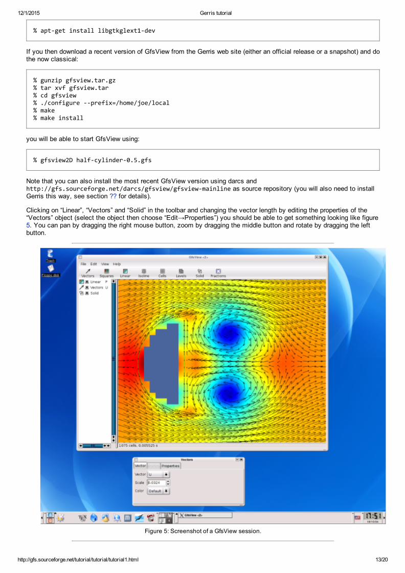
% gfsview2D half‐cylinder‐0.5.gfs
Note that you can also install the most recent GfsView version using darcs andhttp://gfs.sourceforge.net/darcs/gfsview/gfsview‐mainline as source repository (you will also need to installGerris this way, see section ?? for details).
Clicking on “Linear”, “Vectors” and “Solid” in the toolbar and changing the vector length by editing the properties of the“Vectors” object (select the object then choose “Edit→Properties”) you should be able to get something looking like figure5. You can pan by dragging the right mouse button, zoom by dragging the middle button and rotate by dragging the leftbutton.
While by no means complete, you can already do many things with GfsView. I hope it is fairly userfriendly so just playwith it and discover for yourself.
3.3.2 Some postprocessing using gfs2oogl
Gerris comes with a utility called gfs2oogl which converts simulation files to various representations in OOGL format.We are just going to look at two types of representations gfs2oogl can do: scalar field crosssections and vector fields.
First of all, you can access a small summary of the options of gfs2oogl by typing:
% gfs2oogl2D ‐h
By default gfs2oogl will generate the same output as GfsOutputBoundaries like this:
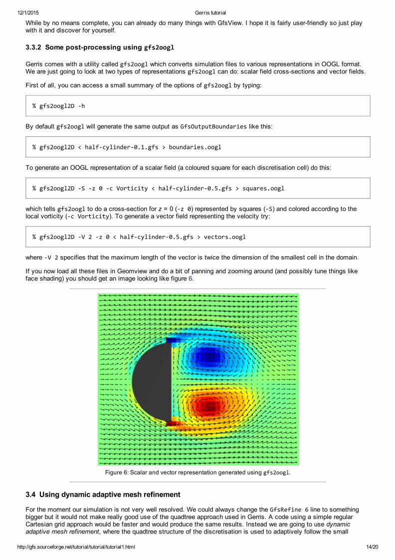
which tells gfs2oogl to do a crosssection for z = 0 (‐z 0) represented by squares (‐S) and colored according to thelocal vorticity (‐c Vorticity). To generate a vector field representing the velocity try:
where ‐V 2 specifies that the maximum length of the vector is twice the dimension of the smallest cell in the domain.
If you now load all these files in Geomview and do a bit of panning and zooming around (and possibly tune things likeface shading) you should get an image looking like figure 6.
Figure 6: Scalar and vector representation generated using gfs2oogl.
3.4 Using dynamic adaptive mesh refinement
For the moment our simulation is not very well resolved. We could always change the GfsRefine 6 line to somethingbigger but it would not make really good use of the quadtree approach used in Gerris. A code using a simple regularCartesian grid approach would be faster and would produce the same results. Instead we are going to use dynamicadaptive mesh refinement, where the quadtree structure of the discretisation is used to adaptively follow the small
structures of the flow, thus concentrating the computational effort on the area where it is most needed.
This is done using yet another object class: GfsAdapt, also derived from GfsEvent. Various criteria can be used todetermine where refinement is needed. In practice, each criterium will be defined through a different object derived fromGfsAdapt. If several GfsAdapt objects are specified in the same simulation file, refinement will occur whenever at leastone of the criteria is verified.
For this first example, we will use a simple criterium based on the local value of the vorticity. A cell will be refinedwhenever
|∇×v|Δ xmax|v|
> δ,
where Δ x is the size of the cell and δ is a userdefined threshold which can be interpreted as the maximum angulardeviation (caused by the local vorticity) of a particle traveling at speed max|v| across the cell. This criterium isimplemented by the GfsAdaptVorticity object.
where mincells specifies the minimum number of cells in the domain, maxcells the maximum number of cells,minlevel the level below which it is not possible to coarsen a cell, maxlevel the level above which it is not possible torefine a cell and cmax the maximum cell cost. The default values are 0 for minlevel and mincells and infinite formaxlevel and maxcells. An important point is that, for the moment, it is not possible to dynamically refine solidboundaries. A simple solution to this restriction is to always refine the solid boundary with the maximum resolution at thestart of the simulation and to restrict the refinement using the maxlevel identifier in GfsAdapt.
What happens if the maximum number of cells is reached? The refinement algorithm will keep the number of cells fixedbut will minimize the maximum cost over all the cells. This can be used for example to run a constantsize simulationwhere the cells are optimally distributed across the simulation domain. This would be done by setting maxcells to thedesired number and cmax to zero.
Following this we can modify our simulation file:
4 3 GfsSimulation GfsBox GfsGEdge GfsTime end = 9 GfsRefine 7 GfsSolid half‐cylinder.gts GfsInit U = 1 # GfsOutputBoundaries boundaries GfsAdaptVorticity istep = 1 maxlevel = 7 cmax = 1e‐2 GfsOutputTime step = 0.02 stdout GfsOutputBalance step = 0.02 stdout GfsOutputProjectionStats step = 0.02 stdout GfsOutputPPM step = 0.02 vorticity.ppm min = ‐100 max = 100 v = Vorticity GfsOutputSimulation step = 0.1 half‐cylinder‐%3.1f.gfs variables = U,V,P GfsOutputTiming start = end stdoutGfsBox left = GfsBoundaryInflowConstant 1 GfsBox GfsBox GfsBox right = GfsBoundaryOutflow 1 2 right2 3 right3 4 right
We have added two lines and commented out (using #) the line outputting the boundaries (we don’t need that anymore,we have the simulation files).
The first line we added says that we want to refine dynamically the mesh through the GfsAdaptVorticity object appliedevery timestep (istep = 1). The δ parameter (cmax) is set to 10−2.
The second line we added is a new GfsOutput object which displays the “balance” of the domain sizes across thedifferent processes (when Gerris is ran in parallel). We will use this to monitor how the number of cells evolves with timeas the simulation refines or coarsens the mesh according to our vorticity criterium.
We can now run this new simulation. If the previous simulation did not complete yet, don’t be afraid to abort it (Ctrl‐C),this one is going to be better (and faster).
% gerris2D half‐cylinder.gfs
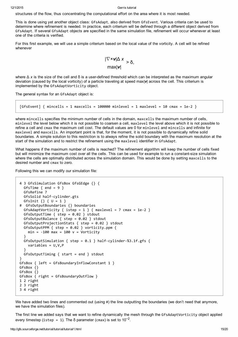
If we now look at the balance summary written by GfsOutputBalance, we see that initially (step: 0) the total number ofcells (on all levels) is 86966, which corresponds to a constant resolution of 4× 27× 27=512× 128. At step 10 the numberof cells is down to 990 with a corresponding increase in computational speed. If we now look at the first simulation file wesaved, using:
we obtain figure 7 showing not only the domain boundaries as usual, but also the boundaries (thin black lines) betweendifferent levels of refinement.
Figure 7: Dynamic adaptive mesh refinement t=0.1
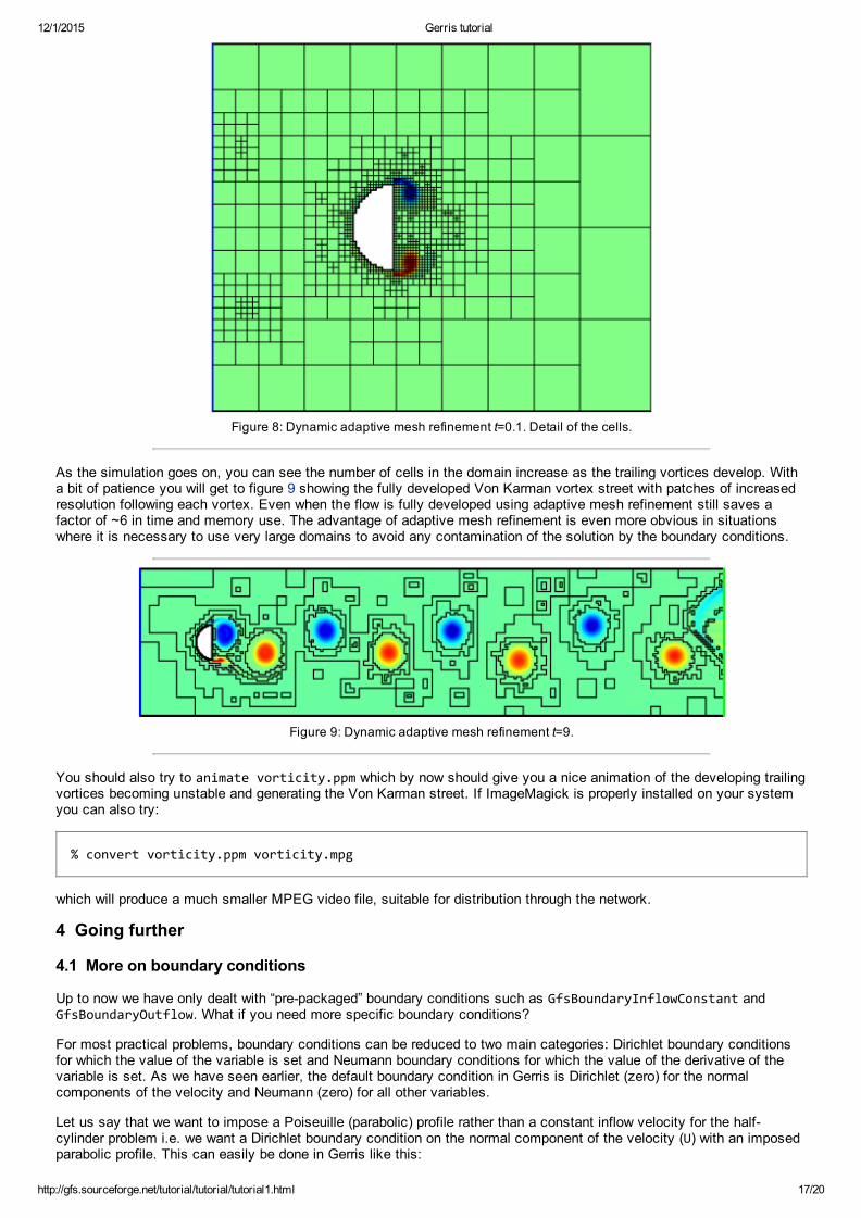
We see that the mesh is very refined around the solid and around the two vortices developing at the trailing edge andvery coarse (one cell per box only) on the downstream part of the domain. If you are not sure what these thin black linesrepresent, just switch on the edge representation in Geomview (using the Inspect→Appearance menu). You will get apicture looking like figure 8, showing all the cells used for the discretisation.
Figure 8: Dynamic adaptive mesh refinement t=0.1. Detail of the cells.
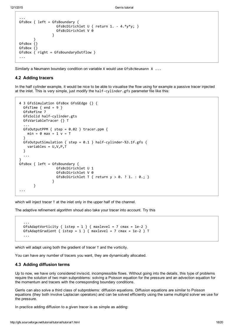
As the simulation goes on, you can see the number of cells in the domain increase as the trailing vortices develop. Witha bit of patience you will get to figure 9 showing the fully developed Von Karman vortex street with patches of increasedresolution following each vortex. Even when the flow is fully developed using adaptive mesh refinement still saves afactor of ~6 in time and memory use. The advantage of adaptive mesh refinement is even more obvious in situationswhere it is necessary to use very large domains to avoid any contamination of the solution by the boundary conditions.
Figure 9: Dynamic adaptive mesh refinement t=9.
You should also try to animate vorticity.ppm which by now should give you a nice animation of the developing trailingvortices becoming unstable and generating the Von Karman street. If ImageMagick is properly installed on your systemyou can also try:
% convert vorticity.ppm vorticity.mpg
which will produce a much smaller MPEG video file, suitable for distribution through the network.
4 Going further
4.1 More on boundary conditions
Up to now we have only dealt with “prepackaged” boundary conditions such as GfsBoundaryInflowConstant andGfsBoundaryOutflow. What if you need more specific boundary conditions?
For most practical problems, boundary conditions can be reduced to two main categories: Dirichlet boundary conditionsfor which the value of the variable is set and Neumann boundary conditions for which the value of the derivative of thevariable is set. As we have seen earlier, the default boundary condition in Gerris is Dirichlet (zero) for the normalcomponents of the velocity and Neumann (zero) for all other variables.
Let us say that we want to impose a Poiseuille (parabolic) profile rather than a constant inflow velocity for the halfcylinder problem i.e. we want a Dirichlet boundary condition on the normal component of the velocity (U) with an imposedparabolic profile. This can easily be done in Gerris like this:
...GfsBox left = GfsBoundary GfsBcDirichlet U return 1. ‐ 4.*y*y; GfsBcDirichlet V 0 GfsBox GfsBox GfsBox right = GfsBoundaryOutflow ...
Similarly a Neumann boundary condition on variable X would use GfsBcNeumann X ...
4.2 Adding tracers
In the half cylinder example, it would be nice to be able to visualise the flow using for example a passive tracer injectedat the inlet. This is very simple, just modify the half‐cylinder.gfs parameter file like this:
4 3 GfsSimulation GfsBox GfsGEdge GfsTime end = 9 GfsRefine 7 GfsSolid half‐cylinder.gts GfsVariableTracer T ... GfsOutputPPM step = 0.02 tracer.ppm min = 0 max = 1 v = T GfsOutputSimulation step = 0.1 half‐cylinder‐%3.1f.gfs variables = U,V,P,T ...GfsBox left = GfsBoundary GfsBcDirichlet U 1 GfsBcDirichlet V 0 GfsBcDirichlet T return y > 0. ? 1. : 0.; ...
which will inject tracer T at the inlet only in the upper half of the channel.
The adaptive refinement algorithm shoud also take your tracer into account. Try this
which will adapt using both the gradient of tracer T and the vorticity.
You can have any number of tracers you want, they are dynamically allocated.
4.3 Adding diffusion terms
Up to now, we have only considered inviscid, incompressible flows. Without going into the details, this type of problemsrequire the solution of two main subproblems: solving a Poisson equation for the pressure and an advection equation forthe momentum and tracers with the corresponding boundary conditions.
Gerris can also solve a third class of subproblems: diffusion equations. Diffusion equations are similar to Poissonequations (they both involve Laplacian operators) and can be solved efficiently using the same multigrid solver we use forthe pressure.
In practice adding diffusion to a given tracer is as simple as adding:
to the parameter file, where 0.01 is the value of the diffusion coefficient.
4.3.1 Boundary conditions for diffusion terms
What if we want to modify the tracer example above so that now the halfcylinder itself is a (diffusive) source of tracerrather than the inlet? We need to be able to impose this boundary condition on the embedded solid surface. Onembedded solids, the default boundary conditions for the diffusion equation is Neumann (zero flux) for tracers andDirichlet (noslip) for the velocity components. To change that use
... GfsVariableTracer T GfsSourceDiffusion T 0.001 GfsSurfaceBc T Dirichlet 1 ...
and change the inlet boundary condition back to
... GfsBox left = GfsBoundary GfsBcDirichlet U 1 GfsBcDirichlet V 0 ...
4.4 Outputs
4.5 Boundary conditions
5 Running Gerris in parallel
6 Learning more
While this tutorial should give you a good overview of Gerris, it is by no means a complete description. To learn more youshould first consult the Gerris Frequently Asked Questions and the Gerris object hierarchy which describes each objectand the corresponding file parameters in more detail.
You should also have a look at the Gerris Examples page for examples of how to use Gerris for a range of problems. Theparameter files are crosslinked with the reference manual.
Another source of more advanced examples is the Gerris test suite.
If things are still unclear you can ask for help on the gfs‐users mailing list. Please note that you first need to subscribeto the list to be able to post messages.
7 Do you want to help?
The idea behind Gerris and other free software projects is that transparency, free exchange of information andcooperation benefit individuals but also society as a whole. If you are a scientist, you know that these same principlesare also keys to the efficiency of Science.
Helping with Gerris development can be done in various ways and aside from giving you this altruistic, warm fuzzy feelingof helping others will also benefit you directly. A few concrete simple ways of helping are (in approximate order ofdifficulty):
Use the code, comment on the problems you find, what you like, don’t like about it.Share your results with other Gerris users, write a web page about the problem you solved using Gerris etc…If you publish papers using Gerris, send me the reference. It is very useful to be able to show evidence of widerusage when seeking continued funding for the project.Also, if Gerris capabilities are central to your article feel free to ask me to be a coauthor on your paper…
Have a look at the Gerris internals (write your own modules) and share them with us.Think of ways to extend Gerris for your own problems, implement them and share them with us (you can count onmy and other developers’ help).