This paper briefly describes the status of Temperature and Chlorophyll-a trend in Kalpakkam Coast, discusses its ecological and temperature impacts recommending measures to achieve long term sustainability using advanced tools like Geographic Information System (GIS). Present study reveals the monthly spatial distribution of Temperature and Chlorophyll-a at Kalpakkam. Transect based in-situ Temperature and Chlorophyll-a collected at 200m, 500m and 1 km distance into the sea was interpolated using the Inverse Distance Weightage (IDW) method in ARC GIS. Data revealed the extent of spatial distribution of thermal effluent in Kalpakkam. It could be found that temperature range of 26.2 – 31.9°C provided substantial Chlorophyll-a concentration between 0.8 – 2.9 mg/m3 for surface and bottom waters.
6
Muthulakshmi.AL et al. Int. Journal of Engineering Research and Applications www.ijera.com ISSN : 2248-9622, Vol. 5, Issue 5, ( Part -5) May 2015, pp.121-126 www.ijera.com 121 | Page GIS based spatial distribution of Temperature and Chlorophyll-a along Kalpakkam, southeast coast of India Muthulakshmi.AL 1 , Usha Natesan 1 , Vincent A. Ferrer 1 , Deepthi.K 1 , Venugopalan.V.P 2 , Narasiman.S.V 2 1 (Centre for Water Resources, Anna University, Chennai, INDIA) 2 (Water and Steam Chemistry Division, Indira Gandhi Centre for Atomic Research, Kalpakkam, INDIA) ABSTRACT This paper briefly describes the status of Temperature and Chlorophyll-a trend in Kalpakkam Coast, discusses its ecological and temperature impacts recommending measures to achieve long term sustainability using advanced tools like Geographic Information System (GIS). Present study reveals the monthly spatial distribution of Temperature and Chlorophyll-a at Kalpakkam. Transect based in-situ Temperature and Chlorophyll-a collected at 200m, 500m and 1 km distance into the sea was interpolated using the Inverse Distance Weightage (IDW) method in ARC GIS. Data revealed the extent of spatial distribution of thermal effluent in Kalpakkam. It could be found that temperature range of 26.2 – 31.9°C provided substantial Chlorophyll-a concentration between 0.8 – 2.9 mg/m 3 for surface and bottom waters. Further, increase of Chlorophyll-a levels did not lead to higher productivity. Combined temperature and chlorophyll a showed little synergistic effects. It is concluded that the effect of thermal discharge from the power plant into the receiving water body is quite localized and productivity of the coastal waters are not affected. From the results obtained, the spatial data has been found to be useful in determining zones of safe use of seawater and to understand the extent of relationship between the relatable parameters. Keywords - Coastal Power Plants, Chlorophyll a, Geographic Information Systems, Temperature, Inverse Distance Weighting (IDW) I. INTRODUCTION Natural water bodies are being used as heat sinks by various industries especially by electric power plants. Thermal effluents released by such plants into the receiving water body, sea or lake can directly and indirectly affect the ecosystem dynamics in the receiving water body. Through its effects are confined to density, temperature is also involved in advective mixing processes and in turn is a major factor in primary production [1]. Seasonal fluctuations in water temperature distribution play an important role in influencing biological processes [2]. In this juncture, the environmental effects of thermal discharge from power stations into coastal and inland water bodies have been the focus of research [3-5]. However in developing countries such as India, this area has only recently attracted significant attention particularly with the advent of larger nuclear and thermal power plants. The Nuclear power plants discharge large amount of heat to cooling water during the process of steam condensation. Nuclear power plants require, on an average about 3 m 3 cooling water per minute per megawatt of electricity (MWe) produced [6]. Since once – through cooling system is the most economical way of condensing the exhaust steam from turbines, there is an increasing tendency for new nuclear power plants to be located in coastal areas, so as to make use of the availability of the abundant seawater for condenser cooling [7]. With an increase in the number of power plants along the coast to meet the growing demands of the society, there is an in comitant increase in the quantity of heated effluents being discharged into coastal marine environments. The marine organisms in the receiving water body may also be entrained into the effluent plume which undergoes a thermal stress on their living and existence. Thus temperature is one of the most important environmental variables which affect the survival, growth and reproduction of aquatic organisms [8-9]. As the heated effluents reaches out to the open sea, they get dispersed spatially over the area depending upon the tidal conditions prevailing over the sea, the direction of the oceanic currents and the wind direction which contributes to the motion of the surface water. Hence it makes it necessary for the temperature to be represented spatially in order to have a clear overview of how the temperature gets dispersed over a period of time. This helps in the assessment of the variation of the temperature RESEARCH ARTICLE OPEN ACCESS
Transcript
Muthulakshmi.AL et al. Int. Journal of Engineering Research and Applications www.ijera.com
ISSN : 2248-9622, Vol. 5, Issue 5, ( Part -5) May 2015, pp.121-126
www.ijera.com 121 | P a g e
GIS based spatial distribution of Temperature and Chlorophyll-a
along Kalpakkam, southeast coast of India
Muthulakshmi.AL1, Usha Natesan
1, Vincent A. Ferrer
1, Deepthi.K
1,
Venugopalan.V.P2, Narasiman.S.V
2
1(Centre for Water Resources, Anna University, Chennai, INDIA)
2(Water and Steam Chemistry Division, Indira Gandhi Centre for Atomic Research, Kalpakkam, INDIA)
ABSTRACT This paper briefly describes the status of Temperature and Chlorophyll-a trend in Kalpakkam Coast, discusses its
ecological and temperature impacts recommending measures to achieve long term sustainability using advanced
tools like Geographic Information System (GIS). Present study reveals the monthly spatial distribution of
Temperature and Chlorophyll-a at Kalpakkam. Transect based in-situ Temperature and Chlorophyll-a collected
at 200m, 500m and 1 km distance into the sea was interpolated using the Inverse Distance Weightage (IDW)
method in ARC GIS. Data revealed the extent of spatial distribution of thermal effluent in Kalpakkam. It could
be found that temperature range of 26.2 – 31.9°C provided substantial Chlorophyll-a concentration between 0.8
– 2.9 mg/m3 for surface and bottom waters. Further, increase of Chlorophyll-a levels did not lead to higher
productivity. Combined temperature and chlorophyll a showed little synergistic effects. It is concluded that the
effect of thermal discharge from the power plant into the receiving water body is quite localized and productivity
of the coastal waters are not affected. From the results obtained, the spatial data has been found to be useful in
determining zones of safe use of seawater and to understand the extent of relationship between the relatable
parameters.
Keywords - Coastal Power Plants, Chlorophyll a, Geographic Information Systems, Temperature, Inverse
Distance Weighting (IDW)
I. INTRODUCTION Natural water bodies are being used as heat
sinks by various industries especially by electric
power plants. Thermal effluents released by such
plants into the receiving water body, sea or lake can
directly and indirectly affect the ecosystem
dynamics in the receiving water body. Through its
effects are confined to density, temperature is also
involved in advective mixing processes and in turn is
a major factor in primary production [1]. Seasonal
fluctuations in water temperature distribution play an
important role in influencing biological processes
[2]. In this juncture, the environmental effects of
thermal discharge from power stations into coastal
and inland water bodies have been the focus of
research [3-5]. However in developing countries
such as India, this area has only recently attracted
significant attention particularly with the advent of
larger nuclear and thermal power plants.
The Nuclear power plants discharge large
amount of heat to cooling water during the process
of steam condensation. Nuclear power plants
require, on an average about 3 m3 cooling water per
minute per megawatt of electricity (MWe) produced
[6]. Since once – through cooling system is the most
economical way of condensing the exhaust steam
from turbines, there is an increasing tendency for
new nuclear power plants to be located in coastal
areas, so as to make use of the availability of the
abundant seawater for condenser cooling [7]. With
an increase in the number of power plants along the
coast to meet the growing demands of the society,
there is an in comitant increase in the quantity of
heated effluents being discharged into coastal marine
environments. The marine organisms in the
receiving water body may also be entrained into the
effluent plume which undergoes a thermal stress on
their living and existence. Thus temperature is one
of the most important environmental variables which
affect the survival, growth and reproduction of
aquatic organisms [8-9].
As the heated effluents reaches out to the open
sea, they get dispersed spatially over the area
depending upon the tidal conditions prevailing over
the sea, the direction of the oceanic currents and the
wind direction which contributes to the motion of
the surface water. Hence it makes it necessary for
the temperature to be represented spatially in order
to have a clear overview of how the temperature gets
dispersed over a period of time. This helps in the
assessment of the variation of the temperature
RESEARCH ARTICLE OPEN ACCESS
Muthulakshmi.AL et al. Int. Journal of Engineering Research and Applications www.ijera.com
ISSN : 2248-9622, Vol. 5, Issue 5, ( Part -5) May 2015, pp.121-126
www.ijera.com 122 | P a g e
derived parameters like DO, salinity etc. With the
advent and development of the various remote
sensing and Geographic information systems, the
spatial mapping of the temperature has found a great
leap in the spatial analysis of the field data. Also the
near shore regions of the sea being a very turbulent
region the data measurement at every region
becomes a tedious one and hence the interpolation of
the measured available data for the entire region
could help in a way to assess the situation therein.
Determining the eutrophication level in a coastal
area depends not only on the vast data obtained, but
also on the distribution of data throughout the
coastal system. Therefore, appropriate methods and
tools are needed to reveal this distribution.
Geographic Information System applications have
the exact features to satisfy this requirement. GIS is
a kind of information system which can perform
functions such as collecting, storing, processing, and
analysing the graphical or non-graphical information
obtained with location-based observations, and it
presents to the user the information as a whole. The
most significant advantage of GIS is that it provides
the resulting desired map by superposing the
distribution maps created with different parameters
within a particular database. For this reason, GIS is
used in many studies related to the management of
natural resources, especially the management of
surface water resources [10 -13].
The present paper has studied the spatial
distribution of temperature and Chlorophyll-a at
Kalpakkam coastal area for different months. The
study locations are provided in Fig. 1. Further, an
attempt has been made to understand the relationship
between temperature and chlorophyll a using the
analysis of GIS.
II. STUDY AREA
The study was carried out in and around the
coastal waters of the IGCAR, Kalpakkam which
houses the Madras Atomic Power Station (MAPS).
The study area extends over a distance of 15 kms
from Sadras in the south to Mahabalipuram in the
north. A schematic representation of the study area
is shown in the Fig 1. The area is an open sandy
coast with negligible tidal currents. MAPS consist
of two units of pressurized heavy water reactors
(PHWR) with an installed capacity of 220 MWe
each down rated to 170 MWe each. It is proposed to
establish a 500 MWe capacity Prototype Fast
Breeder Reactor (PFBR) at about 680 metre south of
MAPS. The power station uses sea water as tertiary
coolant at a maximum design flow rate of 35 m3
s-1
whereas the actual rate varies depending on the
number of units functional at that time. The sea
water is drawn from an offshore well located about
400 m away from the shore through a 50 m deep sub
– seabed tunnel. In order to have a combined
discharge from both PFBR and MAPS an
engineering canal has been constructed. After
passing through the steam condensers and other
auxiliary heat exchangers, the sea water is
discharged onshore through an outfall structure on
the northern side of the jetty into an engineering
canal. The Engineering canal is about 46 metres
wide which runs over a distance of 980 metres and is
constructed using the synthetic material at the
bottom, loaded with stone boulders. Thus the
discharge water from the outfall reaches the sea after
travelling this engineering canal at a fixed point.
Two backwaters drain into the Bay of Bengal in the
vicinity of the power plant viz., Sadras in the south
and Edaiyur in the north.
Fig. 1 Study Area and its Monitoring Sites
III. METHODOLOGY The development of a methodology for the
prediction of chlorophyll a production and
measurement of temperature involved a structured
interdisciplinary approach, which incorporated three
distinct stages: (a) Sampling Strategy, (b) data
collection and analysis and (c) Spatial interpolation
analysis. Each of these stages is discussed below.
3.1. Sampling Strategy
Monthly boat cruises were carried out in the sea
over the period of 12 months from January 2010 to
December 2010 in an area of about 15 (alongshore)
x 1 km into sea. The study area is divided into
twelve transects with three stations in each viz., 200,
500 and 1000 meters. The stations were chosen
based upon the prevailing conditions like
backwaters, thermal mixing point. A total of 72
samples were obtained for each month (Fig. 1). A
schematic representation of the sampling stations
was given in figure 1. Sampling was undertaken
Muthulakshmi.AL et al. Int. Journal of Engineering Research and Applications www.ijera.com
ISSN : 2248-9622, Vol. 5, Issue 5, ( Part -5) May 2015, pp.121-126
www.ijera.com 123 | P a g e
over a tidal cycle, and sampling locations were fixed
using global positioning system (GPS).
Table 1: Study Area Description
Station No. Area Description
Station 1 200m south of Sadras
Station 2 IGCAR township
Station 3 Meyyurkuppam village
Station 4 Periya Odai (South boundary
of IGCAR)
Station 5 200m south of seawall
Station 6 Front of seawall
Station 7 200m north of seawall
Station 8 200m north of Edaiyur
Station 9 Kokillamedeu (North
boundary of IGCAR)
Station 10 Venpurusham
Station 11 200m south of shore temple
(Mahabalipuram)
Station 12 200m north of shore temple
(Mahabalipuram)
3.2. Data Collection and Analysis
Surface and bottom water samples were
collected at 12 locations for a period of one year
(January 2010 – December 2010) throughout the
study area. Table 1 lists the sampling dates and the
number of samples collected during the study. Water
samples were collected fortnightly in precleaned
polythene bottles, and bottom samples were drawn
by using a Niskin water sampler. Samples were kept
in darkness at a low temperature (4 °C), following
collection in order to minimize biological activity.
Water temperature measurements were made using
standard mercury filled centigrade thermometer.
After filtering the water samples through 0.45 μm
Millipore filter paper the Chl-a was analyzed by
spectrophotometry following the method of [14]. For
the spectrophotometric analyses, a double beam UV
Visible Spectrophotometer (Chemito Spectrascan
UV 2600) was used.
3.3. Spatial Interpolation Analysis
There are several spatial interpolation
techniques, including inverse distance weighting
(IDW), radial basic functions, local polynomial
interpolation, etc. [15]. Compared with others, IDW
is the simplest and most practical interpolation
method [16 and 15]. IDW uses the measured values
surrounding the prediction location and assumes that
each measured point has a local influence that
decreases with distance [17 and 15]. Using the factor
scores of VFs as variables, this study applies IDW to
create various continuous surfaces to present the
pollution patterns influenced by each potential
pollution source [16 and 18 - 21]. The data were
subjected to spatial analysis using the Spatial
Analyst module of ArcGIS 9.2. The data at different
points were interpolated adopting the IDW method
which resulted in a more reasonable output.
IV RESULTS AND DISCUSSION Spatial distribution of temperature and
chlorophyll was studied to understand the
relationship between these parameters, especially to
determine at what levels of temperature, the
chlorophyll concentration increases to reach the
level of eutrophication, if any. It is well established
that in brackishwater and seawater systems,
temperature and chlorophyll a is the preferred
parameters that leads to enhanced production, at
times resulting in eutrophication. The data on
temperature and chlorophyll a collected at 36
locations during 2010 were spatially interpolated and
spatial data of temperature and Chlorophyll a for the
year 2010 are given in Fig.2 to 5. The temperatures
were categorized into the classes of low (25.0°C -
27.57°C), normal (27.57°C -30.14°C) and high
(30.14°C -32.7°C). Similarly, Chlorophyll a
concentrations were categorized into the classes of
Low (0.16-1.39 mg/m3), normal (1.39-2.62 mg/m
3)
and high (2.62-3.84 mg/m3).
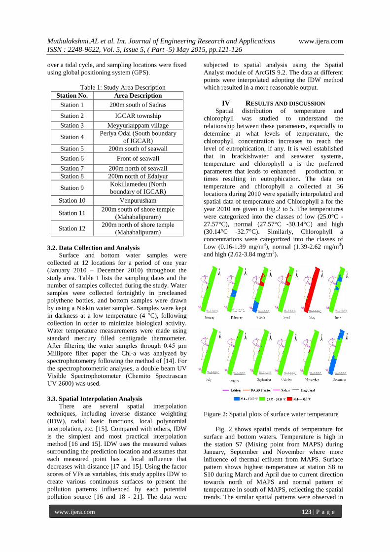
Figure 2: Spatial plots of surface water temperature
Fig. 2 shows spatial trends of temperature for
surface and bottom waters. Temperature is high in
the station S7 (Mixing point from MAPS) during
January, September and November where more
influence of thermal effluent from MAPS. Surface
pattern shows highest temperature at station S8 to
S10 during March and April due to current direction
towards north of MAPS and normal pattern of
temperature in south of MAPS, reflecting the spatial
trends. The similar spatial patterns were observed in
Muthulakshmi.AL et al. Int. Journal of Engineering Research and Applications www.ijera.com
ISSN : 2248-9622, Vol. 5, Issue 5, ( Part -5) May 2015, pp.121-126
www.ijera.com 124 | P a g e
all stations during the month of May. A decline
temperature is noticed in north (Station S1 to S5)
and south (Station S10 to S12) part of Kalpakkam,
whereas middle part (Station S6 to S9) shows
slightly increased temperature. The bottom
temperature showed similar pattern like surface
water temperature. During the month of May, the
plume structure is formed towards north of MAPS
(Station S7 to S12) due to current direction. The
northern part (Station S7 to S12) of the Kalpakkam
shows decline temperature in the month of June
(Fig. 3), whereas lowest temperature pattern were
noticed during December in all stations due to the
effects of monsoon.
Figure 3: Spatial plots of bottom water temperature
Among the 36 sampling stations occupied
during each cruise, a station about 500m south of the
MAPS jetty was not influenced (in terms of
temperature) by the discharge from the power plant.
This station, which represented ambient sea
conditions, was designated as the control station, for
the purpose of determining seasonal variation of
temperature in the coastal waters.
As shown in Fig.4, decline chlorophyll-a
concentration in northeast monsoon and post
monsoon for surface water, exhibit significant trends
in chlorophyll-a. Such declines appear to be
associated with monsoonal activities. Thirty- Six
monitoring stations show decreasing trends in
chlorophyll-a during January. Only one station
exhibit increasing trend at station S8 (Edaiyur
backwater), illustrating the freshwater influx.
Whereas bottom water also shows increased in
chlorophyll a concentration at station S8, associated
with freshwater influence. The final map (Fig. 4 &
5) showing the spatial distribution of coastal
eutrophication based on the distribution maps of the
trophic level, based on annual values for chlorophyll
a in the GIS environment. The map shows that the
trophic level of the Kalpakkam coastal water. The
results prove that coastal water is not affected by
power plant effluents. The concentrations of Chl-a
were the lowest in northeast monsoon, and the
normal concentration in rest of the months (Fig. 5).
Figure 4: Spatial plots of surface water Chlorophyll -
a concentration
Higher Chlorophyll-a concentration were
observed in the Edaiyur (Station S8) than in other
areas of the bay, with maximum during southwest
monsoon. Chlorophyll-a concentration shows two
opposite trends for surface and bottom in station S8.
Approximately all stations do not exhibit significant
trends in Chlorophyll-a during summer. Annual
monthly variations between temperature and
chlorophyll a in all stations are given in Fig. 3. It
shows a pattern with one peak, in all stations during
May month at station S7. The highest temperature
(31.9°C) was recorded in May and the lowest (26.2
°C) in January (Fig. 6 & 7).
Muthulakshmi.AL et al. Int. Journal of Engineering Research and Applications www.ijera.com
ISSN : 2248-9622, Vol. 5, Issue 5, ( Part -5) May 2015, pp.121-126
www.ijera.com 125 | P a g e
Figure 5: Spatial plots of bottom water Chlorophyll-
a concentration
V CONCLUSION
A GIS-based IDW interpolation method was
used to generate spatial trend indicating the spatial
distribution of temperature and chlorophyll a. The
use of spatial data derived from the point data has
been found to be useful in determining the extent of
quantitative spatial distribution of physical
parameters in the coastal waters. The pattern of
spatial distribution of temperature and chlorophyll a
indicated the influence of freshwater influx from
backwaters, thermal effluents from MAPS outfall
and physical parameters like coastal currents on the
zonal spatial distribution of these parameters.
Figure 6: Monthly variation of Temperature and
Chlorophyll-a for surface water
The increase of temperature at station S7 to S9
clearly revealed the effectiveness of thermal
effluents. But the presence of high concentration of
chlorophyll a in seawater revealed that freshwater
influx. Further, information on study area of
seawater with normal temperature and chlorophyll a
can be used of seawater for condenser cooling and
other human related use. The analysis of GIS proved
to be an excellent tool to study the trend of vital
parameter like temperature and chlorophyll a. An
exercise done using this tool to study the effect of
temperature on chlorophyll a revealed that even at
temperature below 31.9°C, normal concentration of
chlorophyll could be achieved indicating that the
coastal waters of Kalpakkam not affected by thermal
effluents. The existence of such a relationship can be
demonstrated using the location specific GIS based
spatial point data, as it clearly indicates the extent of
quantitative spatial distribution of concentrations
and also facilitate better understanding of reality of
correlations between the parameters. A conclusion
section must be included and should indicate clearly
the advantages, limitations, and possible applications
of the paper. Although a conclusion may review the
main points of the paper, do not replicate the abstract
as the conclusion. A conclusion might elaborate on
the importance of the work or suggest applications
and extensions.
Figure 7: Monthly variation of Temperature and
Chlorophyll-a for bottom water
Muthulakshmi.AL et al. Int. Journal of Engineering Research and Applications www.ijera.com
ISSN : 2248-9622, Vol. 5, Issue 5, ( Part -5) May 2015, pp.121-126
www.ijera.com 126 | P a g e
Acknowledgements The authors are thankful to the financial
assistance provided by the Board for Research in
Nuclear Sciences, Government of India.
REFERENCES [1] Langford, T.E, Effects of Thermal
Discharges (London: Elsevier), 1990.
[2] Kinee, O., Marine Ecology. Vol. I,
Environmental Factors Part I (New York:
Wiley Intersciences), 1972.
[3] Dey, W.P, Jinks, S.M, Lauer, G.J., The
316(b) assessment process: evolution
towards a risk-based approach.
Environmental Science & Policy,
3(supplement 1), 2000, 15–23.
[4] Mayhew, D.A., Jensen, L.D., Hanson, D.F,
Muessig, P.H., A comparative review of
entrainment survival studies at power plants
in estuarine environments. Environmental
Science & Policy, 3(supplement 1), 2000,
295–301.
[5] Choi, D.H, Park, J.S, Hwang, C.Y, Huh,
S.H, Cho, C., Effects of thermal effluents
from a power station on bacteria and
heterotrophic nanoflagellates in coastal
waters. Mar. Ecol. Prog. Ser., 2002, 229, 1–
10.
[6] Schubel, J.R., Marcy, Jr., B.C. (Eds.), Power
Plant Entrainment—A Biological
Assessment. Academic Press, Inc., New
York, 1978, pp. 19–189.
[7] Winter, J.V., Conner, D.A., Power Plant
Siting. Van Nostrand Reinhold
Environmental Engineering Series. Litton
Educational Publishing, Inc., New York,
1978, pp. 61–81.
[8] Kinne, O. (Ed.), ‘Marine Ecology’
Environmental Factors Part I, vol. 1. Wiley,
New York, 1970, pp. 321–363.
[9] Langford, T.E.L., Ecological effects of
thermal discharges. Elsevier Applied Science
Publishers Ltd., England, 1990, pp. 28–103.
[10] Xu, F.L, Tao S, Dawson, R.W, Li, B.G., A
GIS-Based Method of Lake Eutrophication
Assesment. Ecological Modelling 2001, 144:
231- 244.
[11] Akdeniz, S., Water quality assessment of
Lake Uluabat and analysis of geographic
information system, M.Sc. Thesis (In
Turkish). Uludağ Üniversitesi, Fen Bilimleri
Enstitüsü, Bursa, 2005, 126p.
[12] Küçükball, A, Karaer, F, Akdeniz, S, Ertürk,
A., The use of geographic information
system for natural resource management (in
Turkish). In: Symposium on modern
methods in science, 272-279, Kocaeli, 2005,
16-18 November 2005.
[13] Karaer, F, Küçükballi, A., Monitoring of
water quality and assessment of organic
pollution load .n the Nilüfer Stream, Turkey,
Environmental Monitoring and Assessment,
2006, 114 (1-3):391-417.
[14] Strickland, S. C., Parsons, T. R., A Practical