School of Economics and Finance

Working Paper No. 757 October 2015 ISSN 1473-0278

Zeyyad Mandalinci and Haroon Mumtaz

Global Economic Divergence and Portfolio Capital Flows to Emerging Markets

Global Economic Divergence and Portfolio Capital Flowsto Emerging Markets

Zeyyad Mandalincia, Haroon Mumtaza

aSchool of Economics and Finance, Queen Mary University of London, UK

October 7, 2015

Abstract

This paper studies the role of global and regional variations in economic activityand policy in developed world in driving portfolio capital flows (PCF) to emergingmarkets (EMs) in a Factor Augmented Vector Autoregressive (FAVAR) framework.Results suggest that PCFs to EMs depend mainly on economic activity at the globallevel and monetary policy in America, positively on the former and negatively on thelatter. In contrast, economic activity and policy shocks in Europe and Asia contributesignificantly less to variations in PCFs to EMs. Hence, PCFs are driven by not onlycommon shocks across all developed countries, but also variations in specific regions.This implies that economic divergence in the developed world can have significanteffects on EMs via PCFs.

Keywords: Portfolio Capital Flows; Bayesian Analysis, Factor Model, VAR, Emerg-ing Markets.JEL Classification: C11, C32, E30, E52, E58, F32.

1 Introduction

Divergence in economic activity and policy has been a widely debated topic across policymakers and academics. In particular, the issue have become more relevant in the after-math of the global financial crisis. United States economy has experienced a strongerrebound than other developed economies in Europe and Asia. Hence, after three roundsof Quantitative Easing, the United States Federal Reserve (FED) terminated its assetpurchasing programme in 2014, whereas in Asia and Europe, central banks scaled uptheir measures to further loose monetary policy in the face of possible deflation. As aresult, FED is expected to raise its policy rate in late 2015, whereas in Europe and Asiapolicy rates are expected to remain at historically low levels. In this current environmentof economic divergence in the developed world, a great uncertainty for EMs is how capitalflows will be affected. In this paper, we study the importance of variations in activity andpolicy at different global hierarchical levels to help shed light on the possible implicationsof economic divergence on PCFs to EMs.

Existing Literature on PCFs suggest that interest rates and activity in the developedworld are relevant drivers of PCFs.1 However, considering the increasing level of inter-national real and financial linkages, a common drawback of previous studies is that they

1See for instance, Chuhan et al. (1998), Taylor & Sarno (1997), Forbes & Warnock (2012).

1

do not account for the fact that variations in key variables are increasingly due to factorsthat originate at the global or regional level rather than at national level.2 For instance,Kose et al. (2012) study global business cycle synchronization in a dynamic factor modeland find convergence in business cycles of industrial countries. They argue that countryspecific variations have become less important over time. So, before examining the roleof a particular variable of a country in driving PCFs to EMs, one has to account for thefact that variations in the given variable may be due to variations at a higher hierarchicallevel. Hence, one has to decompose the variations in country specific variables into varia-tions at different hierarchical levels. Clearly, this is especially important if the objectiveis to study the implications of economic divergence in developed countries on EMs, viathe impact of global and region specific shocks on PCFs as in here.

To study the global and regional variations in economic activity and policy in thedeveloped world on PCFs to EMs, this paper employs a Factor-Augmented Vector Au-toregressive (FAVAR) Model. Variations in countries in North America, Europe and AsiaPacific are decomposed into variations at global, regional and idiosyncratic levels, andincorporated in a VAR, together with a factor representing common variations in PCFsto different countries, to study the role of shocks originating at different hierarchical levelsin driving flows.3

Results indicate, global activity shocks are important drivers for PCFs. Adverse globalactivity shocks have significant negative effects on PCFs. Hence, PCFs are found to bepro-cyclical with respect to global economic activity. At the regional level, contractionaryAmerican and Asian monetary policy shocks have significant negative impact on PCFs.Furthermore, forecast error variance and historical decompositions indicate that the mostimportant drivers are global activity shocks and American monetary policy shocks. Over-all, since there is heterogeneity in the importance of variations at different levels andregions, economic divergence have implications for PCFs and hence EMs. In particular,since the single most important driver of PCFs is American interest rates, a respectiveincrease may have significant negative effects on PCFs. However, since PCFs are pro-cyclical with respect to global economic activity, a rebound in global economic growthmay help rebalance the possible fall in PCFs.

The following Section describes the econometric model and the estimation; Section 3presents the dataset, Section 4 illustrates the results and Section 5 concludes.

2 Econometric Model

Early literature categorize the drivers of capital flows as global push factors and country-specific pull factors.4 Similarly, we consider the following representation for PCFs,

pcfit = βiFpcft + vit, vit = ρ

it(L)vit + eit, eit ∼ N(0, σ2vi)

where F pcft and vit represent the common component driven by push factors acrossflows to different countries, and country-specific component driven by pull factors ofcountry i respectively. Push factors include activity and policy variables at global and

2See for instance, Hirata et al. (2012), Diebold et al. (2008), Thorsrud (2013).3During the paper, we use America and North America, Asia and Asia Pacific interchangeably.4See for instance, Fernandez-Arias & Montiel (1996), Fernandez-Arias (1996), Mody et al. (2001),

Edison & Warnock (2008).

2

regional levels. Push factors and the common component of capital flows are assumed tohave the following FAVAR representation,

vixtF ytF ptF rtF pcft

= c+B(L)

vixt−1F yt−1F pt−1F rt−1F pcft−1

+ ut (1)

vixtXyt

Xpt

Xrt

pcft

=

1 0 0 0 00 Λy 0 0 00 0 Λp 0 00 0 0 Λr 00 0 0 0 Λpcf

vixtF ytF ptF rtF pcft

+ vt (2)

where ut ∼ N(0, A−1Q(A−1)′), vt = ρ(L)vt + evt with evt ∼ N(0, R), X representdata vectors on which different factors load, pcft collects data on PCFs to different coun-tries, F pcft represents the common component of capital flows across countries, and vixtrepresents the VIX index as a known driver. y, p and r represent real growth, inflationand short interest rates respectively. For y, p and r, we extract factors at global andregional levels; North America, Europe and Asia Pacific. For instance for y,

Xyt = ΛyF yt + vyt =

Λy11 DAmerica,y

1 DEurope,y1 DAsia,y

1

Λy21 DAmerica,y2 DEurope,y

2 DAsia,y2

......

......

Λy.1 DAmerica,y. DEurope,y

. DAsia,y.

FGlobal,yt

FAmerica,yt

FEurope,yt

FAsia,yt

+ vyt

DLocation,yi =

{Λi if country i is in Location0 if country i is not in Location

}Notice that the global factor loads on all growth variables in all regions, whereas

regional factors load only on the variables in their respective regions. Similar to Mumtaz& Surico (2009), the loading of each factor on the first variable at the respective region isset to 1 and that variable is only allowed to load on the respective factor for identification.5

The identification of the structural shocks is carried out by imposing a specific order-ing on the FAVAR variables. For all regions we order the factors as F y, F p, F r, whichidentifies monetary policy shocks within each region, similar to Christiano et al. (1999)and Primiceri (2005). We order capital flows factor last following the common conventionin the FAVAR literature regarding the ordering of the fast-moving variables like flows.67 We order vix first, assuming that it represents uncertainty shocks, similar to Leduc &Liu (2015).8 Regions are ordered with respect to their economic size; Global, America,Europe and Asia Pacific. Overall, we identify regional monetary policy shocks, as well asuncertainty and portfolio capital flows shocks. We interpret structural shocks to growthand inflation factors as activity shocks, given that the existing literature consider and

5We use the codes provided by Binning (2013) for identification.6We have tested for the number of common factors in pcf following Bai & Ng (2002), and concluded

that a single factor is adequate.7See for instance, Bernanke et al. (2005).8We have also experimented by ordering vix last and observed that the findings do not change.

3

Figure 1: Convergence: Recursive Means of Factors

decompose the variation in these indicators as supply and demand shocks.9 To obtain thecontemporaneous impact matrix A−1, we apply cholesky decomposition on the variancecovariance matrix of FAVAR residuals.

We set the FAVAR lag length to 2. Estimation has been carried out by Markov ChainMonte Carlo (MCMC) methods, Gibbs Sampling similar to Mumtaz & Surico (2009) andLiu et al. (2014). Minnesota priors for FAVAR parameters10 and uninformative priorsfor other parameters have been implemented. Furthermore, we use principle componentestimates to obtain the starting values for the FAVAR coeffi cients and the factors.

The estimation steps start with setting the priors and starting values, then respectivelydrawing factor loadings, factors following Carter & Kohn (1994), FAVAR coeffi cients,FAVAR variance covariance matrix, variable/country specific component autoregressivecoeffi cients, variable/country specific component variances. We repeat sampling stepsuntil convergence, with 50000 replications and 40000 as burn in.

3 Dataset

Table 1 outlines the list of countries included in the model for PCFs and Fundamentals.In total 21 emerging market countries are included for PCFs, and 16 developed countriesfor fundamentals. The sample period is 1988Q1 - 2014Q3. The data for the fundamentalsare from Datastream, The Organization for Economic Co-operation and Development(OECD), International Monetary Fund International Financial Statistics (IFS). Existingdata from mentioned sources is supplemented with the dataset from Mandalinci (2014)who uses various data sources and interpolation procedures to interpolate missing quar-terly observations, in particular to construct quarterly PCFs variables. Final constructed

9See for instance, Bayoumi (1992) and Bayoumi & Eichengreen (1994).10Using dummy observations as in Banbura et al. (2007) and Banbura et al. (2010).

4

Figure 2: Estimated Factors

pcf variables reflect the net purchases of portfolio equity and debt instruments of non-residents from residents. We normalize flows by nominal gdp for each country.

For growth indicators, we use real gdp, composite leading indicators and industrialproduction. For inflation, we include consumer price index, producer price index, gdpdeflator and core consumer price index for each country depending on the data availability.For short term interest rates, policy rates, deposit rates and 3 month Treasury-bill rateshave been used. As a robustness check, we also augment the benchmark model with realequity prices of national stock markets. Yearly percentage changes are used for growthand price measures, whereas quarterly growth rates are for stock prices. Growth andinflation indicators are seasonally adjusted; and all variables are standardized.

Table 1: List of Countriespcf Fundamentals

Argentine Hungary Pakistan Taiwan U.States Italy U.KingdomBrazil India Peru Thailand Canada Netherlands JapanChina Indonesia Philippines Turkey Austria Norway AustraliaChile Korea Poland Germany Spain N.ZealandColombia Malaysia Romania France SwedenEgypt Mexico S.Africa Finland Switzerland

4 Results

Figure 1 depicts the recursive means of estimated factors. Draws obtained from the simu-lations do not portray any shifts, indicating convergence of the MCMC algorithm. Figure2 presents the estimated factors with 68% quantiles from their posterior distributions.Overall, the factors portray variations that are in line with prior expectations for all

5

Figure 3: Selected Impulse Response Functions

regions. For instance, they indicate the dramatic fall in economic growth and inflationduring the recent global financial crisis, as well as historically low interest rates in theaftermath. Evidence of the early 90s slowdown in the America and the late 90s EastAsian crisis are present in the regional growth factors. Also, the factors suggest that therebound in growth has been stronger in America compared to a much weaker rebound inEurope and to a lesser extend Asia Pacific, which is not surprising given the Europeansovereign debt crisis. Regarding capital flows, we observe significant falls in 1995 Mexi-can and 1997-8 East Asian Crisis and Russian default; but they have been much smallerin absolute terms than the fall during the recent global financial crisis. Moreover, therebound in capital flows to EMs in the aftermath of the crisis is captured by the commonfactor.

Figure 3 presents the Impulse Response Functions (IRFs) following Global activity,American and Asian monetary policy and uncertainty shocks. Depicted shocks are theones that PCFs respond strongest among all structural shocks. Starting with the globalactivity shocks, from the responses of PCFs one can argue that PCFs are pro-cyclicalwith respect to the global activity. In other words, adverse activity shocks, which affectglobal growth negatively, result in significant falls in PCFs. Also, one can see that a risein interest rates in North America causes a brief fall in growth and also cause a significantfall in PCFs. The long debated price puzzle11 appear for America, as prices increase. Inthe fourth row, a rise in short interest rates in Asia Pacific causes growth and prices togo down in the short run as expected, and also results in a significant fall in PCFs. Thismay reflect the fact that currencies of the countries in this region are widely consideredto be the short side of the carry trade activity, like Australia and Japan. Hence a rise inshort rates may reduce flows to EMs as borrowing costs rise for carry traders. Turning tothe uncertainty shock, the responses of all model variables except interest rates in Asia,

11As discussed in Sims (1992) and Bernanke et al. (2005).

6

Figure 4: FEVD of pcf - Global and Regional Aggregates

are significant and negative, including PCFs.

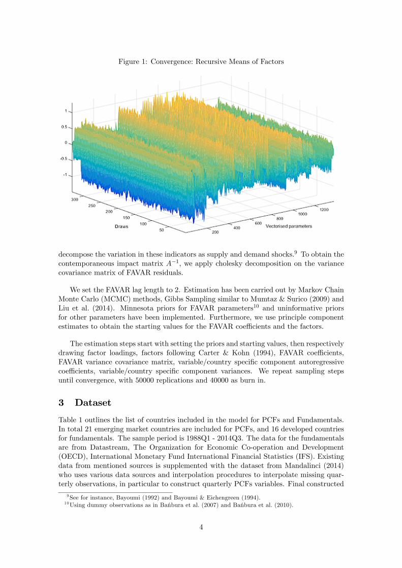
To examine whether variations at the global or regional levels are the major drivingforces behind PCFs, we calculate Forecast Error Variance Decomposition (FEVD) ofPCFs. Figure 4 presents the contribution of structural shocks, aggregated within differ-ent hierarchical levels, on PCFs at different horizons, together with the contribution ofuncertainty shocks. One can clearly see that flows are driven mainly by the variation inAmerica and Globe, whereas contemporaneously and in one quarter uncertainty shocksplay a significant role.

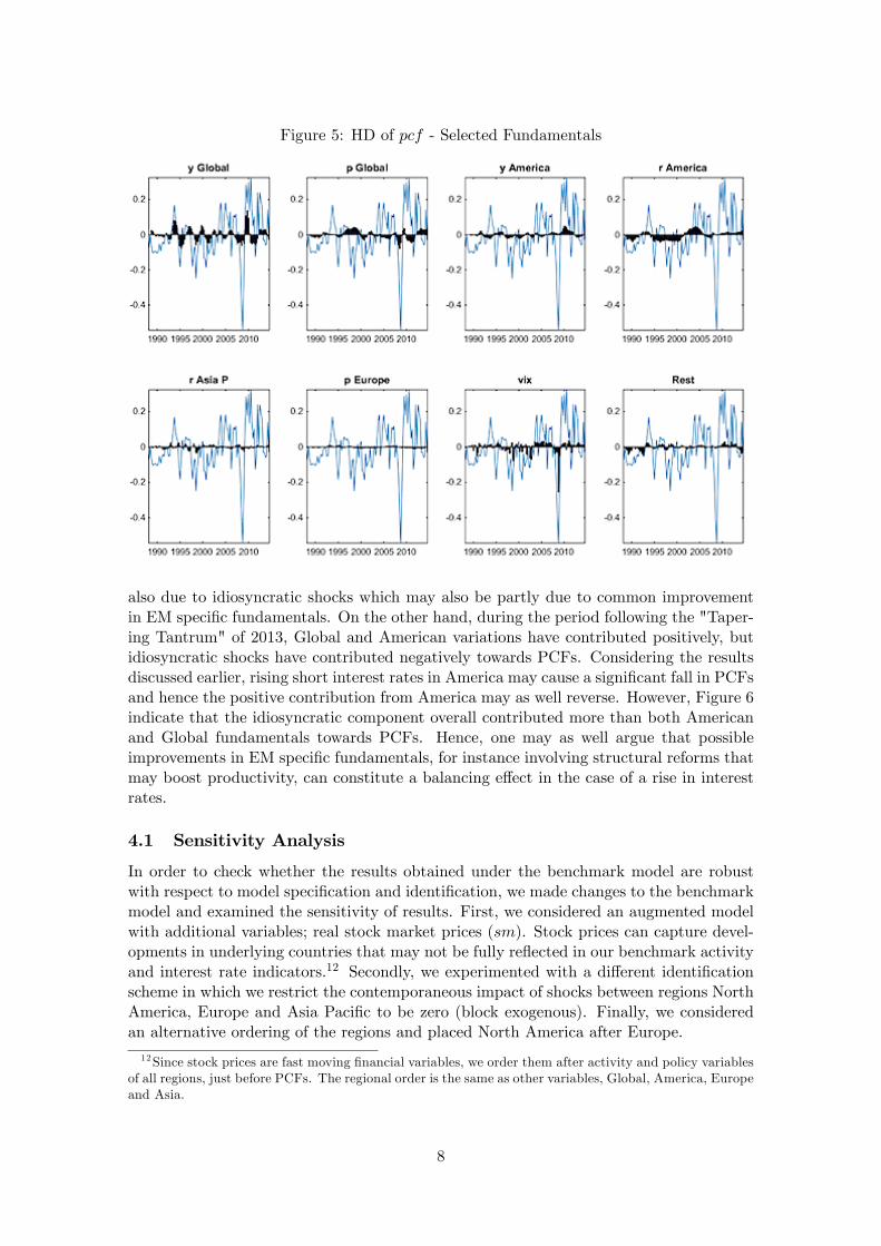
Figure 5 presents the Historical Decomposition (HD) of PCFs to selected fundamen-tals, to better understand the contributions of different variables to PCFs during thesample period. As expected from the earlier results, shocks to Global activity and Amer-ican short interest rates seem to have contributed the most towards PCFs. Even thoughIRFs indicate that Asian interest rates shock significantly affect PCFs, its contributionhad been minimal over the sample period. Results indicate that uncertainty shocks havecontributed significantly to the fall in PCFs in 1998 Russian default and 2008 global fi-nancial crisis episodes. Also, reduced uncertainty during 2003-2007 period seem to haveplayed an important role in the notable surge in PCFs to EMs.

Figure 6 plots the historical contributions of idiosyncratic, uncertainty and aggregateglobal and regional shocks’ contributions to PCFs. Results indicate that Global andAmerican shocks have contributed most towards PCFs during the sample period consid-ered here. As expected from the results of the FEVDs, variations in activity and interestrates in Europe and Asia have contributed little towards PCFs overall. Towards the endof the sample period, results indicate that the significant rebound in PCFs to EMs follow-ing the global financial crisis was mostly due to Global and American fundamentals, but

7

Figure 5: HD of pcf - Selected Fundamentals

also due to idiosyncratic shocks which may also be partly due to common improvementin EM specific fundamentals. On the other hand, during the period following the "Taper-ing Tantrum" of 2013, Global and American variations have contributed positively, butidiosyncratic shocks have contributed negatively towards PCFs. Considering the resultsdiscussed earlier, rising short interest rates in America may cause a significant fall in PCFsand hence the positive contribution from America may as well reverse. However, Figure 6indicate that the idiosyncratic component overall contributed more than both Americanand Global fundamentals towards PCFs. Hence, one may as well argue that possibleimprovements in EM specific fundamentals, for instance involving structural reforms thatmay boost productivity, can constitute a balancing effect in the case of a rise in interestrates.

4.1 Sensitivity Analysis

In order to check whether the results obtained under the benchmark model are robustwith respect to model specification and identification, we made changes to the benchmarkmodel and examined the sensitivity of results. First, we considered an augmented modelwith additional variables; real stock market prices (sm). Stock prices can capture devel-opments in underlying countries that may not be fully reflected in our benchmark activityand interest rate indicators.12 Secondly, we experimented with a different identificationscheme in which we restrict the contemporaneous impact of shocks between regions NorthAmerica, Europe and Asia Pacific to be zero (block exogenous). Finally, we consideredan alternative ordering of the regions and placed North America after Europe.

12Since stock prices are fast moving financial variables, we order them after activity and policy variablesof all regions, just before PCFs. The regional order is the same as other variables, Global, America, Europeand Asia.

8

Figure 6: HD of pcf - Global and Regional Aggregates

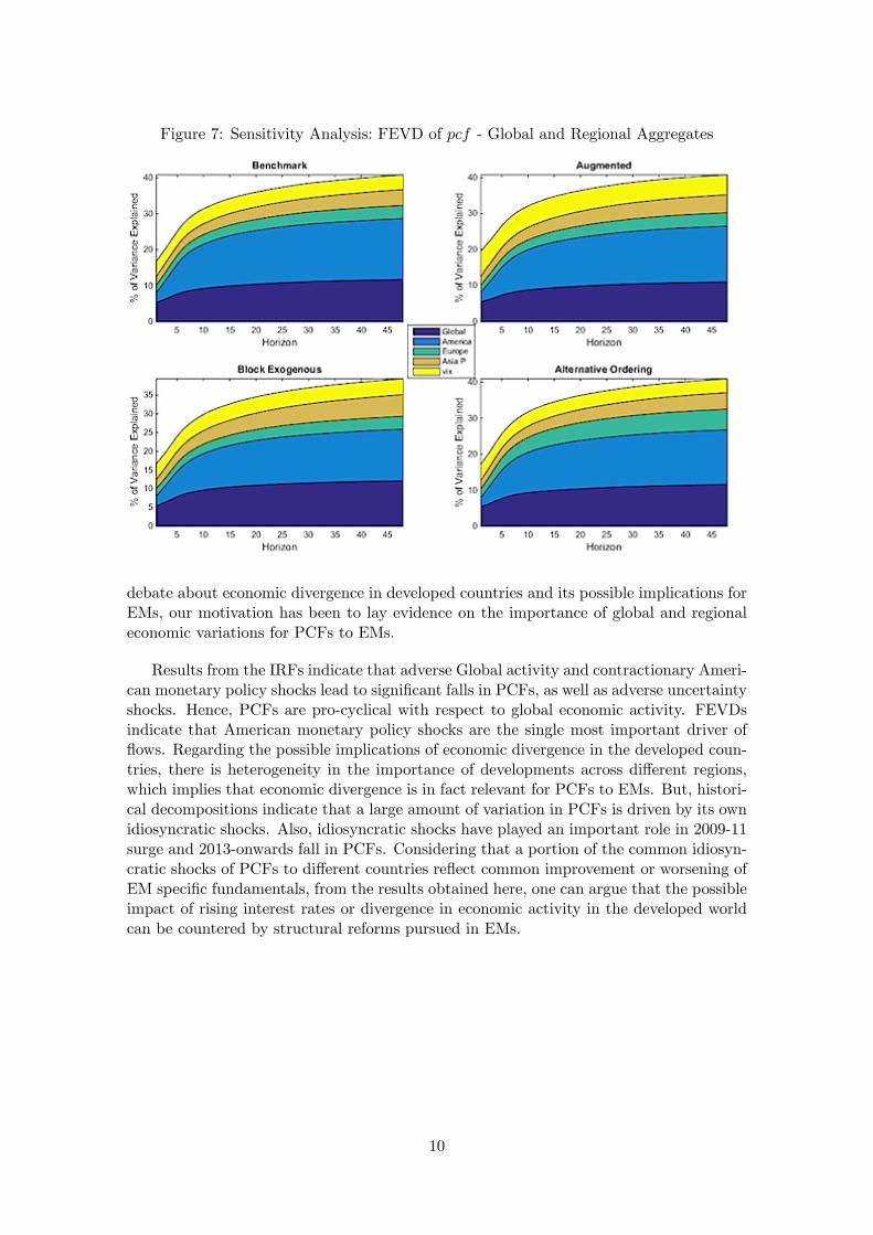
Table 2 presents the correlation of estimated factors in the benchmark model with theones obtained in the augmented model with real stock prices. The factors are essentiallyidentical, except a slight difference for the growth factor of Asia Pacific. In this case, theaugmented model factor suggests slightly stronger real growth in Asia Pacific during 1996-1999. Figure 7 presents the FEVDs for PCFs under the benchmark and alternative casesconsidered. With stock prices, there is little change in the importance of fundamentals.Only notable difference is that the importance of uncertainty shocks increases slightly.Considering the case with a block exogenous contemporaneous impact matrix, Asia Pacificgains more importance and variations originating in North America slightly less. But theorder of importance is still very similar, with American and Global fundamentals beingthe most important followed by Asia and Europe. Finally, when we reverse the orderingof North America and Europe, the importance of European fundamentals become higher,but again much lower than Global and North America. Overall, results are found to berobust with respect to changes in the model specification and identification assumptions.

Table 2: Correlation of Estimated Factors under Benchmark and Augmented Modely Global y Amer. y Europe y Asia P r Global r Amer. r Europe0.9994 0.9952 0.9995 0.7549 0.9985 0.9977 0.9977r Asia P p Global p Amer. p Europe p Asia P pcf0.9900 0.9991 0.9996 0.9985 0.9994 0.9840

5 Conclusion

This paper contributes to the literature by examining the role of global and regional activ-ity and monetary policy shocks in driving PCFs to EMs. We have constructed a FAVARmodel with PCFs and fundamentals that reflect activity and monetary policy shocks atdifferent hierarchical levels, as well as uncertainty shocks. In the light of the on-going

9

Figure 7: Sensitivity Analysis: FEVD of pcf - Global and Regional Aggregates

debate about economic divergence in developed countries and its possible implications forEMs, our motivation has been to lay evidence on the importance of global and regionaleconomic variations for PCFs to EMs.

Results from the IRFs indicate that adverse Global activity and contractionary Ameri-can monetary policy shocks lead to significant falls in PCFs, as well as adverse uncertaintyshocks. Hence, PCFs are pro-cyclical with respect to global economic activity. FEVDsindicate that American monetary policy shocks are the single most important driver offlows. Regarding the possible implications of economic divergence in the developed coun-tries, there is heterogeneity in the importance of developments across different regions,which implies that economic divergence is in fact relevant for PCFs to EMs. But, histori-cal decompositions indicate that a large amount of variation in PCFs is driven by its ownidiosyncratic shocks. Also, idiosyncratic shocks have played an important role in 2009-11surge and 2013-onwards fall in PCFs. Considering that a portion of the common idiosyn-cratic shocks of PCFs to different countries reflect common improvement or worsening ofEM specific fundamentals, from the results obtained here, one can argue that the possibleimpact of rising interest rates or divergence in economic activity in the developed worldcan be countered by structural reforms pursued in EMs.

10

References

Bai, J., & Ng, S. (2002). Determining the number of factors in approximate factor models.Econometrica, 70 (1), 191—221.

Banbura, M., Giannone, D., & Reichlin, L. (2007). Bayesian vars with large panels. CEPRDiscussion Paper No. DP6326, Centre for Economic Policy Research.

Banbura, M., Giannone, D., & Reichlin, L. (2010). Large bayesian vector auto regressions.Journal of Applied Econometrics, 25 (1), 71—92.

Bayoumi, T. (1992). The effect of the erm on participating economies. Staff Papers-International Monetary Fund , (pp. 330—356).

Bayoumi, T., & Eichengreen, B. (1994). One money or many?: Analyzing the prospectsfor monetary unification in various parts of the world , vol. 76. International FinanceSection, Department of Economics, Princeton University Princeton.

Bernanke, B. S., Boivin, J., & Eliasz, P. (2005). Measuring the effects of monetary policy:a factor-augmented vector autoregressive (favar) approach. The Quarterly Journal ofEconomics, 120 (1), 387—422.

Binning, A. (2013). Underidentified svar models: A framework for combining short andlong-run restrictions with sign-restrictions. Working Papers 14, Norges Bank.

Carter, C. K., & Kohn, R. (1994). On gibbs sampling for state space models. Biometrika,81 (3), 541—553.

Christiano, L., Eichenbaum, M., & Evans, C. (1999). Monetary policy shocks: What havewe learned and to what end? Handbook of macroeconomics, 1 , 65—148.

Chuhan, P., Claessens, S., & Mamingi, N. (1998). Equity and Bond Flows to Latin Amer-ica and Asia: The Role of Global and Country Specific Factors. Journal of DevelopmentEconomics, 55 (2), 439—463.

Diebold, F., Li, C., & Yue, V. (2008). Global yield curve dynamics and interactions: Adynamic nelson—siegel approach. Journal of Econometrics, 146 (2), 351—363.

Edison, H., & Warnock, F. (2008). Cross-Border Listings, Capital Controls, and EquityFlows to Emerging Markets. Journal of International Money and Finance, 27 (6),1013—1027.

Fernandez-Arias, E. (1996). The new wave of private capital inflows: push or pull?Journal of development economics, 48 (2), 389—418.

Fernandez-Arias, E., & Montiel, P. J. (1996). The Surge in Capital Inflows to DevelopingCountries: an Analytical Overview. The World Bank Economic Review , 10 (1), 51—77.

Forbes, K., & Warnock, F. (2012). Capital Flow Waves: Surges, Stops, Flight, andRetrenchment. Journal of International Economics, 88 (2), 235—251.

Hirata, H., Kose, M., Otrok, C., & Terrones, M. (2012). Global House Price Fluctuations:Synchronization and Determinants. NBER Working Papers 18362, National Bureau ofEconomic Research, Inc.

11

Kose, M., Otrok, C., & Prasad, E. (2012). Global business cycles: Convergence or decou-pling?*. International Economic Review , 53 (2), 511—538.

Leduc, S., & Liu, Z. (2015). Uncertainty shocks are aggregate demand shocks. WorkingPaper Series 12/10, Federal Reserve Bank of San Francisco.

Liu, P., Mumtaz, H., & Theophilopoulou, A. (2014). The transmission of internationalshocks to the uk. estimates based on a time-varying factor augmented var. Journal ofInternational Money and Finance, 46 , 1—15.

Mandalinci, Z. (2014). Determinants, Dynamics and Implications of International Port-folio Capital Flows. Ph.D. thesis, University of Warwick, Coventry, UK.

Mody, A., Taylor, M. P., & Kim, J. Y. (2001). Modelling Fundamentals for ForecastingCapital Flows to Emerging Markets. International Journal of Finance & Economics,6 (3), 201—216.

Mumtaz, H., & Surico, P. (2009). The transmission of international shocks: A factor-augmented var approach. Journal of Money, Credit and Banking , 41 (s1), 71—100.

Primiceri, G. E. (2005). Time varying structural vector autoregressions and monetarypolicy. The Review of Economic Studies, 72 (3), 821—852.

Sims, C. (1992). Interpreting the macroeconomic time series facts: The effects of monetarypolicy. European Economic Review , 36 (5), 975—1000.

Taylor, M., & Sarno, L. (1997). Capital flows to developing countries: long-and short-termdeterminants. The World Bank Economic Review , 11 (3), 451—470.

Thorsrud, L. (2013). Global and regional business cycles-shocks and propagations. NorgesBank Working Papers 2013/08, Norges Bank.

12

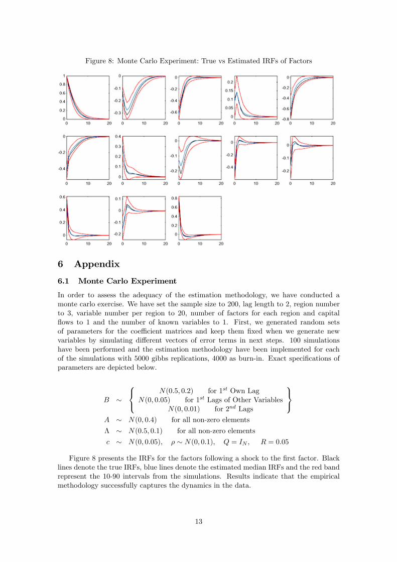
Figure 8: Monte Carlo Experiment: True vs Estimated IRFs of Factors

6 Appendix

6.1 Monte Carlo Experiment

In order to assess the adequacy of the estimation methodology, we have conducted amonte carlo exercise. We have set the sample size to 200, lag length to 2, region numberto 3, variable number per region to 20, number of factors for each region and capitalflows to 1 and the number of known variables to 1. First, we generated random setsof parameters for the coeffi cient matrices and keep them fixed when we generate newvariables by simulating different vectors of error terms in next steps. 100 simulationshave been performed and the estimation methodology have been implemented for eachof the simulations with 5000 gibbs replications, 4000 as burn-in. Exact specifications ofparameters are depicted below.

B ∼

N(0.5, 0.2) for 1st Own Lag

N(0, 0.05) for 1st Lags of Other VariablesN(0, 0.01) for 2nd Lags

A ∼ N(0, 0.4) for all non-zero elements

Λ ∼ N(0.5, 0.1) for all non-zero elements

c ∼ N(0, 0.05), ρ ∼ N(0, 0.1), Q = IN , R = 0.05

Figure 8 presents the IRFs for the factors following a shock to the first factor. Blacklines denote the true IRFs, blue lines denote the estimated median IRFs and the red bandrepresent the 10-90 intervals from the simulations. Results indicate that the empiricalmethodology successfully captures the dynamics in the data.

13

This working paper has been produced bythe School of Economics and Finance atQueen Mary University of London

School of Economics and FinanceQueen Mary University of LondonMile End RoadLondon E1 4NSTel: +44 (0)20 7882 7356Fax: +44 (0)20 8983 3580Web: www.econ.qmul.ac.uk/research/workingpapers/

Copyright © 2015 Zeyyad Mandalinci and Haroon MumtazAll rights reserved