HAL Id: inria-00451193 https://hal.inria.fr/inria-00451193v3 Submitted on 22 Aug 2012 HAL is a multi-disciplinary open access archive for the deposit and dissemination of sci- entific research documents, whether they are pub- lished or not. The documents may come from teaching and research institutions in France or abroad, or from public or private research centers. L’archive ouverte pluridisciplinaire HAL, est destinée au dépôt et à la diffusion de documents scientifiques de niveau recherche, publiés ou non, émanant des établissements d’enseignement et de recherche français ou étrangers, des laboratoires publics ou privés. Global solutions to rough differential equations with unbounded vector fields Antoine Lejay To cite this version: Antoine Lejay. Global solutions to rough differential equations with unbounded vector fields. Cather- ine Donati-Martin and Antoine Lejay and Alain Rouault. Séminaire de Probabilités XLIV, 2046, Springer, pp.215-246, 2012, Lecture Notes in Mathemics, 978-3-642-27460-2. <10.1007/978-3-642- 27461-9_11>. <inria-00451193v3>
Transcript
HAL Id: inria-00451193https://hal.inria.fr/inria-00451193v3
Submitted on 22 Aug 2012
HAL is a multi-disciplinary open accessarchive for the deposit and dissemination of sci-entific research documents, whether they are pub-lished or not. The documents may come fromteaching and research institutions in France orabroad, or from public or private research centers.
L’archive ouverte pluridisciplinaire HAL, estdestinée au dépôt et à la diffusion de documentsscientifiques de niveau recherche, publiés ou non,émanant des établissements d’enseignement et derecherche français ou étrangers, des laboratoirespublics ou privés.
Global solutions to rough differential equations withunbounded vector fields
Antoine Lejay
To cite this version:Antoine Lejay. Global solutions to rough differential equations with unbounded vector fields. Cather-ine Donati-Martin and Antoine Lejay and Alain Rouault. Séminaire de Probabilités XLIV, 2046,Springer, pp.215-246, 2012, Lecture Notes in Mathemics, 978-3-642-27460-2. <10.1007/978-3-642-27461-9_11>. <inria-00451193v3>
Global solutionsto rough differential equationswith unbounded vector fields∗
Antoine Lejay†
July 8, 2011
Abstract
We give a sufficient condition to ensure the global existence of asolution to a rough differential equation whose vector field has a lineargrowth. This condition is weaker than the ones already given and maybe used for geometric as well as non-geometric rough paths with valuesin any suitable (finite or infinite dimensional) space. For this, we studythe properties the Euler scheme as done in the work of A.M. Davie.
1 IntroductionInitiated a decade ago, the theory of rough paths imposed itself as a con-venient tool to define stochastic calculus with respect to a large class ofstochastic processes out of the range of semi-martingales (fractional Brown-ian motion, ...) and also allows one to define pathwise stochastic differentialequations [6, 8, 10,11,15,17,18].∗This work has been supported by the ANR ECRU founded by the French Agence
Nationale pour la Recherche. The author is also indebted to Massimiliano Gubinelli forinteresting discussions about the topic. The author also wish to thank the anonymousreferee for having suggested some improvements in the introduction.†Project-team TOSCA, Institut Elie Cartan Nancy (Nancy-Université, CNRS, IN-
RIA), Boulevard des Aiguillettes B.P. 239 F-54506 Vandœuvre-lès-Nancy, France. E-mail:[email protected]
1
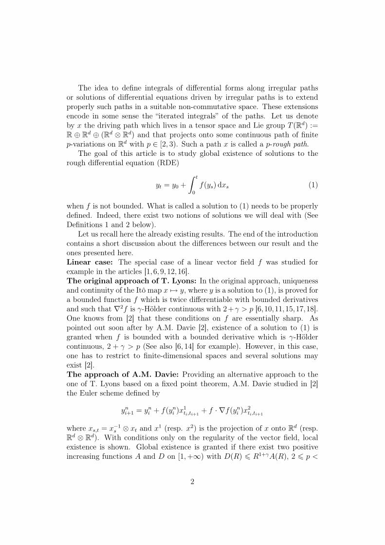
The idea to define integrals of differential forms along irregular pathsor solutions of differential equations driven by irregular paths is to extendproperly such paths in a suitable non-commutative space. These extensionsencode in some sense the “iterated integrals” of the paths. Let us denoteby x the driving path which lives in a tensor space and Lie group T (Rd) :=R ⊕ Rd ⊕ (Rd ⊗ Rd) and that projects onto some continuous path of finitep-variations on Rd with p ∈ [2, 3). Such a path x is called a p-rough path.
The goal of this article is to study global existence of solutions to therough differential equation (RDE)
yt = y0 +
∫ t
0
f(ys) dxs (1)
when f is not bounded. What is called a solution to (1) needs to be properlydefined. Indeed, there exist two notions of solutions we will deal with (SeeDefinitions 1 and 2 below).
Let us recall here the already existing results. The end of the introductioncontains a short discussion about the differences between our result and theones presented here.Linear case: The special case of a linear vector field f was studied forexample in the articles [1, 6, 9, 12,16].The original approach of T. Lyons: In the original approach, uniquenessand continuity of the Itô map x 7→ y, where y is a solution to (1), is proved fora bounded function f which is twice differentiable with bounded derivativesand such that ∇2f is γ-Hölder continuous with 2+γ > p [6,10,11,15,17,18].One knows from [2] that these conditions on f are essentially sharp. Aspointed out soon after by A.M. Davie [2], existence of a solution to (1) isgranted when f is bounded with a bounded derivative which is γ-Höldercontinuous, 2 + γ > p (See also [6, 14] for example). However, in this case,one has to restrict to finite-dimensional spaces and several solutions mayexist [2].The approach of A.M. Davie: Providing an alternative approach to theone of T. Lyons based on a fixed point theorem, A.M. Davie studied in [2]the Euler scheme defined by
yni+1 = yni + f(yni )x1ti,ti+1
+ f · ∇f(yni )x2ti,ti+1
where xs,t = x−1s ⊗ xt and x1 (resp. x2) is the projection of x onto Rd (resp.
Rd ⊗ Rd). With conditions only on the regularity of the vector field, localexistence is shown. Global existence is granted if there exist two positiveincreasing functions A and D on [1,+∞) with D(R) 6 R1+γA(R), 2 6 p <
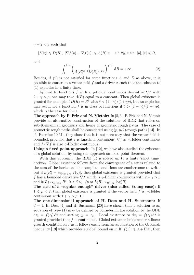
Besides, if (2) is not satisfied for some functions A and D as above, it ispossible to construct a vector field f and a driver x such that the solution to(1) explodes in a finite time.
Applied to functions f with a γ-Hölder continuous derivative ∇f with2 + γ > p, one may take A(R) equal to a constant. Then global existence isgranted for example if D(R) = Rδ with δ < (1+γ)/(1+γp), but an explosionmay occur for a function f is in class of functions if δ > (1 + γ)/(1 + γp),which is the case for δ = 1.The approach by P. Friz and N. Victoir: In [5,6], P. Friz and N. Victoirprovide an alternative construction of the solutions of RDE that relies onsub-Riemannian geodesics and hence of geometric rough paths. The case ofgeometric rough paths shall be considered using (p, p/2)-rough paths [14]. In[6, Exercise 10.61], they show that it is not necessary that the vector field isbounded, provided that f is Lipschitz continuous, ∇f is γ-Hölder continuousand f · ∇f is also γ-Hölder continuous.Using a fixed point approach: In [12], we have also studied the existenceof a global solution, by using the approach on fixed point theorem.
With this approach, the RDE (1) is solved up to a finite “short time”horizon. Global existence follows from the convergence of a series related tothe sum of the horizons. The complete conditions are cumbersome to write,but if h(R) = sup|y|6R |f(y)|, then global existence is granted provided thatf has a bounded derivative ∇f which is γ-Hölder continuous with 2 + γ > pand h(R) ∼R→∞ Rδ, 0 < δ 6 1/p or h(R) ∼R→∞ log(R).The case of a “regular enough” driver (also called Young case): If1 6 p < 2, then global existence is granted if the vector field f is γ-Höldercontinuous with 1 + γ > p [13].The one-dimensional approach of H. Doss and H. Sussmann: Ifd = 1, H. Doss [4] and H. Sussmann [20] have shown that a solution to anequation of type (1) may be defined by considering the solution to the ODEdzt = f(zt) dt and setting yt = zxt . Local existence to dzt = f(zt) dt isgranted provided that f is continuous. Global existence holds under a lineargrowth condition on f as it follows easily from an application of the Gronwallinequality [19] which provides a global bound on z: If |f(z)| 6 A+B|z|, then
3
|zt| 6 (|z0| + At) exp(Bt) for any t > 0. This approach may be generalizedfor a multi-dimensional driver x when f has vanishing Lie brackets.
The situation is more intricate when x lives in a space of dimension biggerthan 2. In particular, the asymptotic behavior of ∇f plays a fundamentalrole.
If x is a p-rough path (a rough path of finite p-variation) with p ∈ [2, 3),then for any function ϕ of finite p/2-variations with values in Rd ⊗ Rd, z =x + ϕ is also a p-rough path. In addition, as shown in [14] for the generalcase, the solution to yt = y0 +
∫ t0f(ys) dzs is also solution to
yt = y0 +
∫ t
0
f(ys) dxs +
∫ t
0
f · ∇f(ys) dϕs. (3)
Consider any rough path z living above the path 0 on Rd with ϕ(t) = ctfor a matrix c (if c is anti-symmetric, then such a rough path is the limitof a sequence of smooth paths lifted in the tensor space by their iteratedintegrals). Then y is solution to
yt = y0 +
∫ t
0
f · ∇f(ys)c ds.
Thus, explosion may occurs according to the behavior of f ·∇f . In particular,f may grow linearly, but f ·∇f may grow faster that linearly, and an explosionmay occur. Of course, if ∇f is bounded and f grows linearly, then f · ∇falso grows linearly.
Example 1 (M. Gubinelli). Consider the solution y of the RDE yt = a +∫ t0f(ys) dxs living in R2 and driven by the rough path xt = (1, 0, (1 ⊗ 1)t)
with values in 1⊕R⊕ (R⊗R). This rough path lies above the constant pathat 0 ∈ R and has only a pure area part which proportional to t. Note thatthis rough path can only be seen as a p-rough path with p > 2 [11]. Theny is also a solution to yt = a +
has a quadratic growth. Take the initial point a = (a1, 0) with a1 > 0. Then(yt)2 = 0 and (yt)1 = a1 +
∫ t0(ys)
21 ds so that (yt)1 → +∞ in finite time equal
to 1/a1. This proves that explosion may occur in a finite time.
4
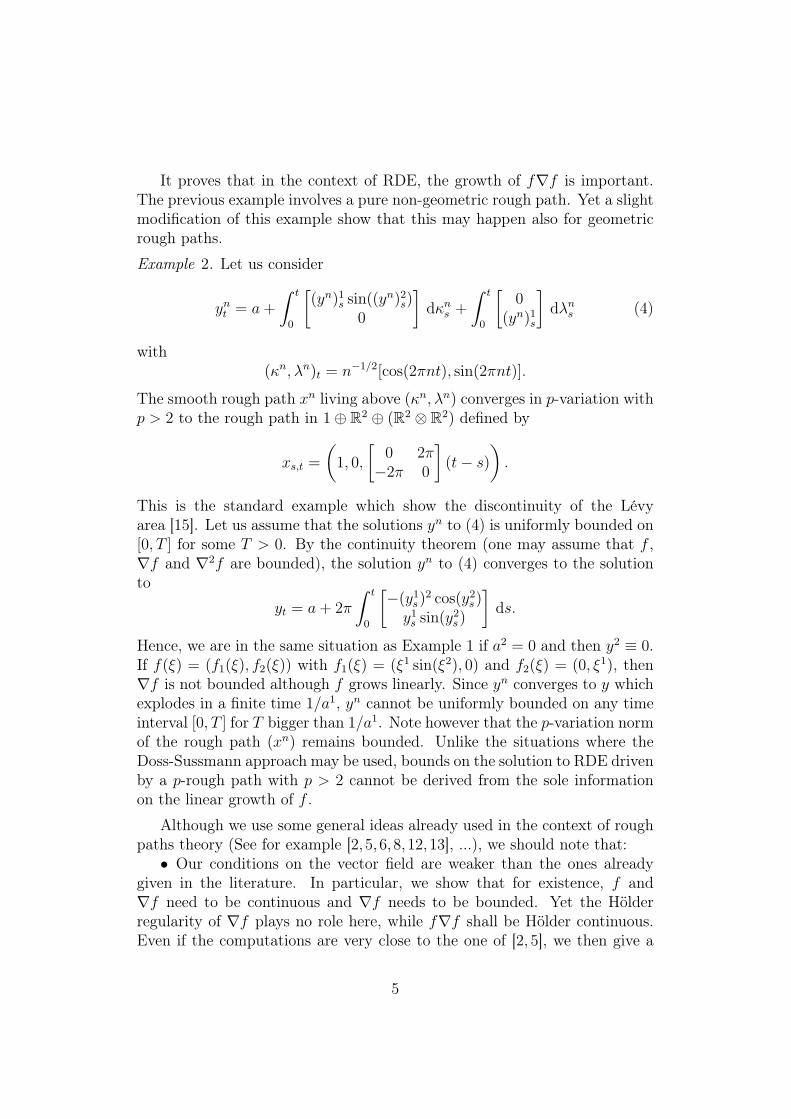
It proves that in the context of RDE, the growth of f∇f is important.The previous example involves a pure non-geometric rough path. Yet a slightmodification of this example show that this may happen also for geometricrough paths.
Example 2. Let us consider
ynt = a+
∫ t
0
[(yn)1
s sin((yn)2s)
0
]dκns +
∫ t
0
[0
(yn)1s
]dλns (4)
with(κn, λn)t = n−1/2[cos(2πnt), sin(2πnt)].
The smooth rough path xn living above (κn, λn) converges in p-variation withp > 2 to the rough path in 1⊕ R2 ⊕ (R2 ⊗ R2) defined by
xs,t =
(1, 0,
[0 2π−2π 0
](t− s)
).
This is the standard example which show the discontinuity of the Lévyarea [15]. Let us assume that the solutions yn to (4) is uniformly bounded on[0, T ] for some T > 0. By the continuity theorem (one may assume that f ,∇f and ∇2f are bounded), the solution yn to (4) converges to the solutionto
yt = a+ 2π
∫ t
0
[−(y1
s)2 cos(y2
s)y1s sin(y2
s)
]ds.
Hence, we are in the same situation as Example 1 if a2 = 0 and then y2 ≡ 0.If f(ξ) = (f1(ξ), f2(ξ)) with f1(ξ) = (ξ1 sin(ξ2), 0) and f2(ξ) = (0, ξ1), then∇f is not bounded although f grows linearly. Since yn converges to y whichexplodes in a finite time 1/a1, yn cannot be uniformly bounded on any timeinterval [0, T ] for T bigger than 1/a1. Note however that the p-variation normof the rough path (xn) remains bounded. Unlike the situations where theDoss-Sussmann approach may be used, bounds on the solution to RDE drivenby a p-rough path with p > 2 cannot be derived from the sole informationon the linear growth of f .
Although we use some general ideas already used in the context of roughpaths theory (See for example [2, 5, 6, 8, 12, 13], ...), we should note that:• Our conditions on the vector field are weaker than the ones already
given in the literature. In particular, we show that for existence, f and∇f need to be continuous and ∇f needs to be bounded. Yet the Hölderregularity of ∇f plays no role here, while f∇f shall be Hölder continuous.Even if the computations are very close to the one of [2, 5], we then give a
5
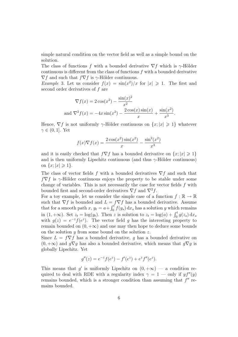
simple natural condition on the vector field as well as a simple bound on thesolution.The class of functions f with a bounded derivative ∇f which is γ-Höldercontinuous is different from the class of functions f with a bounded derivative∇f and such that f∇f is γ-Hölder continuous.Example 3. Let us consider f(x) = sin(x2)/x for |x| > 1. The first andsecond order derivatives of f are
∇f(x) = 2 cos(x2)− sin(x)2
x2
and ∇2f(x) = −4x sin(x2)− 2 cos(x) sin(x)
x+
sin(x2)
x3.
Hence, ∇f is not uniformly γ-Hölder continuous on {x; |x| > 1} whateverγ ∈ (0, 1]. Yet
f(x)∇f(x) =2 cos(x2) sin(x2)
x− sin2(x2)
x3
and it is easily checked that f∇f has a bounded derivative on {x; |x| > 1}and is then uniformly Lipschitz continuous (and thus γ-Hölder continuous)on {x; |x| > 1}.The class of vector fields f with a bounded derivatives ∇f and such thatf∇f is γ-Hölder continuous enjoys the property to be stable under somechange of variables. This is not necessarily the case for vector fields f withbounded first and second-order derivatives ∇f and ∇2f .For a toy example, let us consider the simple case of a function f : R → Rsuch that ∇f is bounded and L = f∇f has a bounded derivative. Assumethat for a smooth path x, yt = a+
∫ t0f(ys) dxs has a solution y which remains
in (1,+∞). Set zt = log(yt). Then z is solution to zt = log(a) +∫ t
0g(zs) dxs
with g(z) = e−zf(ez). The vector field g has the interesting property toremain bounded on (0,+∞) and one may then hope to deduce some boundson the solution y from some bound on the solution z.Since L = f∇f has a bounded derivative, g has a bounded derivative on(0,+∞) and g∇g has also a bounded derivative, which means that g∇g isglobally Lipschitz. Yet
g′′(z) = e−zf(ez)− f ′(ez) + ezf ′′(ez).
This means that g′ is uniformly Lipschitz on (0,+∞) — a condition re-quired to deal with RDE with a regularity index γ = 1 — only if yf ′′(y)remains bounded, which is a stronger condition than assuming that f ′′ re-mains bounded.
6
This kind of computations may be carried to the multi-dimensional caseusing polar coordinates and an exponential change of variable of the radialcomponent.This explains the failure of the attempt carried by some persons, includingthe author of the present article, to get a global bound by such a changeof variable under the sole assumption that ∇f is uniformly γ-Hölder andbounded.• The condition on the vector field appears naturally when one uses the
approach by the Euler scheme proposed by A.M. Davie in [2]. This is notthe case when one uses the notion of solution proposed by T. Lyons becausethe term f∇f is somewhat hidden in the cross iterated integral between thesolution y and the driver x. The idea used in this article to get a globalbound in closely related to the one in [12] where a fixed point approach wasused. Yet in this article [12], we did not succeed article to obtain a globalbound in a general. In addition, the superfluous assumption on the Hölderregularity of ∇f was used and necessary.• The use of sub-Riemaniann geodesics and the reduction to smooth
drivers was the core ideas of [5, 6]. Here, there is no need to restrict to ge-ometric rough paths and the results may be used for any finite-dimensionalBanach spaces and even infinite-dimensional in some cases. Hence, the struc-ture of the underlying spaces plays no role here.Example 4. The most natural example of a non-geometric rough path isthe one B living above a d-dimensional Brownian path W with B1 = Wand B2,i,j
s,t =∫ ts(W i
r −W is) dBj
r . Here the integral has to be understood inthe Itô sense. A geometric rough path B may be constructed above theBrownian path W with B1 = W and B2,i,j
s,t =∫ ts(W i
r −W is)◦ dW j
r , where thestochastic integral is the Stratonovich one. Hence, B and B are linked byB2,i,js,t = B2,i,j
s,t + 12(t− s)δi,j. RDE driven by B correspond to Itô SDE while
the ones driven by B corresponds to Stratonovich SDE.When one use the Brownian rough path B, the Euler scheme presentedhere corresponds indeed to the Milstein scheme. In the very beginning ofrough paths theory, the rate of convergence in this case has been studiedby J. Gaines and T. Lyons [7] with aim at developing simulation algorithmswith adaptative stepsize.In view of (3), the regularity condition on f∇f is also the one which is neces-sary to deal with a non-geometric p-rough path seen as a (p, p/2)-geometricrough path using the decomposition of the space introduced in [14].• The notion of solution to a RDE introduced by T. Lyons [15] cannot be
used here (See Definition 1), so that we use the notion of solution introducedby A.M. Davie in [2] (see Definition 2) which is similar to the one proposed
7
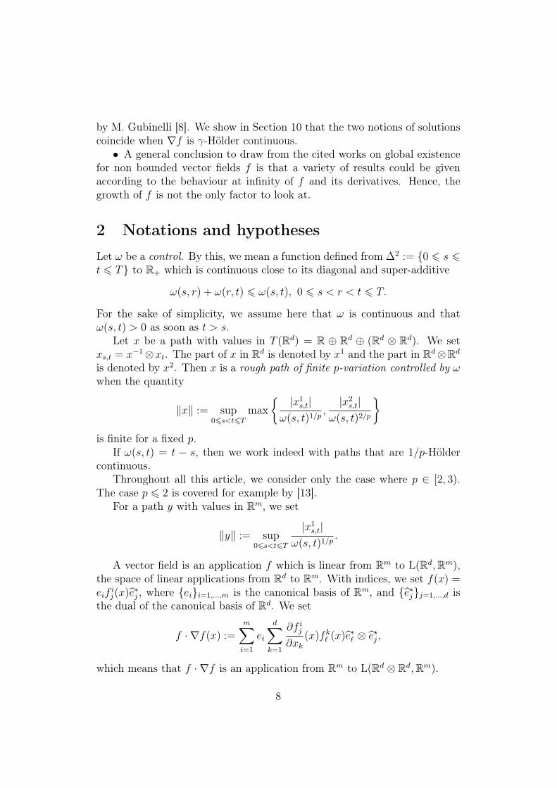
by M. Gubinelli [8]. We show in Section 10 that the two notions of solutionscoincide when ∇f is γ-Hölder continuous.• A general conclusion to draw from the cited works on global existence
for non bounded vector fields f is that a variety of results could be givenaccording to the behaviour at infinity of f and its derivatives. Hence, thegrowth of f is not the only factor to look at.
2 Notations and hypothesesLet ω be a control. By this, we mean a function defined from ∆2 := {0 6 s 6t 6 T} to R+ which is continuous close to its diagonal and super-additive
ω(s, r) + ω(r, t) 6 ω(s, t), 0 6 s < r < t 6 T.
For the sake of simplicity, we assume here that ω is continuous and thatω(s, t) > 0 as soon as t > s.
Let x be a path with values in T (Rd) = R ⊕ Rd ⊕ (Rd ⊗ Rd). We setxs,t = x−1⊗xt. The part of x in Rd is denoted by x1 and the part in Rd⊗Rd
is denoted by x2. Then x is a rough path of finite p-variation controlled by ωwhen the quantity
‖x‖ := sup06s<t6T
max
{ |x1s,t|
ω(s, t)1/p,|x2s,t|
ω(s, t)2/p
}is finite for a fixed p.
If ω(s, t) = t − s, then we work indeed with paths that are 1/p-Höldercontinuous.
Throughout all this article, we consider only the case where p ∈ [2, 3).The case p 6 2 is covered for example by [13].
For a path y with values in Rm, we set
‖y‖ := sup06s<t6T
|x1s,t|
ω(s, t)1/p.
A vector field is an application f which is linear from Rm to L(Rd,Rm),the space of linear applications from Rd to Rm. With indices, we set f(x) =eif
ij(x)e∗j , where {ei}i=1,...,m is the canonical basis of Rm, and {e∗j}j=1,...,d is
the dual of the canonical basis of Rd. We set
f · ∇f(x) :=m∑i=1
ei
d∑k=1
∂f ij∂xk
(x)fk` (x)e∗` ⊗ e?j ,
which means that f · ∇f is an application from Rm to L(Rd ⊗ Rd,Rm).
8
Hypothesis 1. The function f is continuously differentiable from Rm toL(Rd,Rm) and is such that ∇f is bounded and F (x) := f(x) · ∇f(x) isγ-Hölder continuous with norm Hγ(F ) from Rm to L(Rm ⊗ Rd,Rm).
Note that this hypothesis is slightly different from the one given usually toprove existence to solutions of RDE where it is assumed that ∇f is γ-Höldercontinuous.
Hypothesis 2. We assume that p ∈ [2, 3) and that θ := (2 + γ)/p is greaterthan 1.
Definition 1 (Solution in the sense of Lyons). We call by a solution to (1)in the sense of Lyons the projection onto Rm of a rough path z of finitep-variations controlled by ω with values in T (Rm ⊕ Rd) which solves thefollowing equation
zt = z0 +
∫ t
0
g(zs) dzs, (5)
where z projects onto T (Rd) as x, onto Rm as y, and g is the differential formg(y, x) = dx+f(y) dx. The integral in (5) shall be understood as the “roughintegral”, that is as an integral in the sense of rough path.
Note that the definitions of z involves the “cross-iterated integrals” be-tween x and y, and requires that the derivative of f is γ-Hölder continuous.
Under Hypothesis 1, it is not compulsory that ∇f is γ-Hölder continuous,so that we shall use another notion of solution, since we cannot use a fixedpoint theorem that relies on the definition of a rough integral.
3 Solution in the sense of DavieThe notion of solution of (1) we use is the notion of solution in the sense ofDavie, introduced in [2].
Definition 2 (Solution in the sense of Davie). A solution of (1) in the sense ofDavie is a continuous path y from [0, T ] to Rm of finite p-variation controlledby ω such that for some constant L,
|yt − ys −D(s, t)| 6 Lω(s, t)θ, ∀(s, t) ∈ ∆2 (6)
withD(s, t) = f(ys)x
1s,t + F (ys)x
2s,t.
The next propositions, which assume the existence of a solution in thesense of Davie, will be proved below in Section 4
9
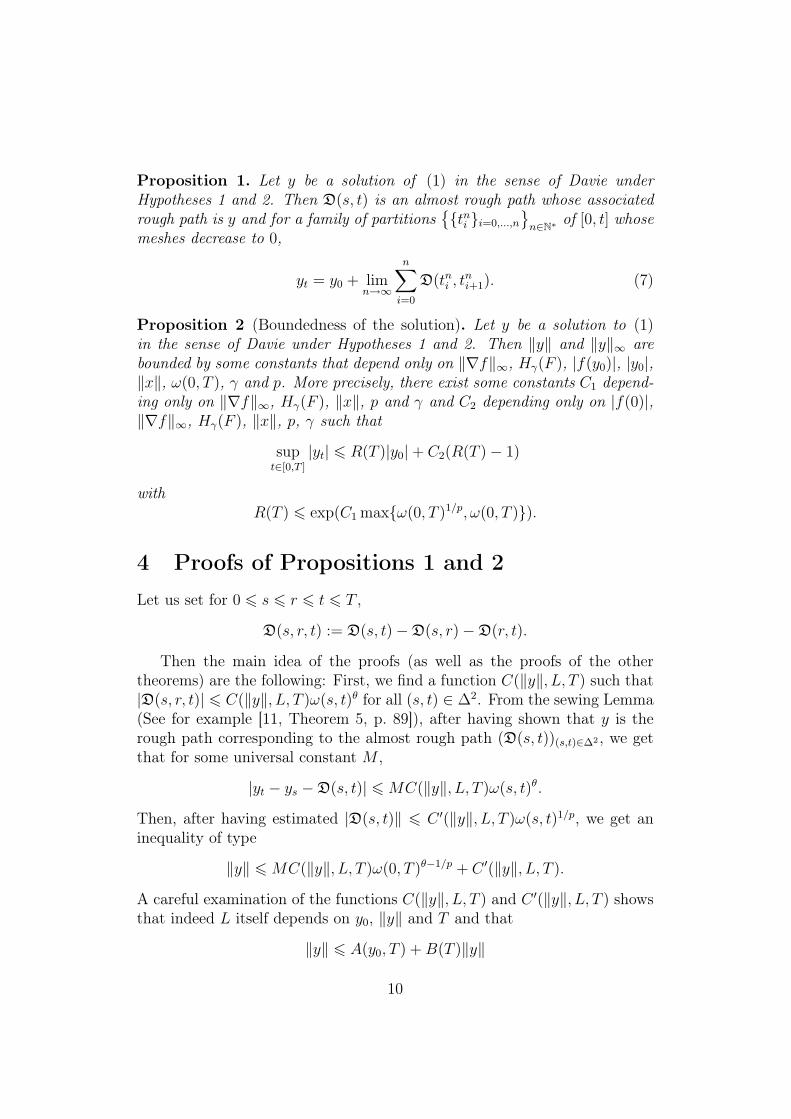
Proposition 1. Let y be a solution of (1) in the sense of Davie underHypotheses 1 and 2. Then D(s, t) is an almost rough path whose associatedrough path is y and for a family of partitions
{{tni }i=0,...,n
}n∈N∗ of [0, t] whose
meshes decrease to 0,
yt = y0 + limn→∞
n∑i=0
D(tni , tni+1). (7)
Proposition 2 (Boundedness of the solution). Let y be a solution to (1)in the sense of Davie under Hypotheses 1 and 2. Then ‖y‖ and ‖y‖∞ arebounded by some constants that depend only on ‖∇f‖∞, Hγ(F ), |f(y0)|, |y0|,‖x‖, ω(0, T ), γ and p. More precisely, there exist some constants C1 depend-ing only on ‖∇f‖∞, Hγ(F ), ‖x‖, p and γ and C2 depending only on |f(0)|,‖∇f‖∞, Hγ(F ), ‖x‖, p, γ such that
supt∈[0,T ]
|yt| 6 R(T )|y0|+ C2(R(T )− 1)
withR(T ) 6 exp(C1 max{ω(0, T )1/p, ω(0, T )}).
4 Proofs of Propositions 1 and 2Let us set for 0 6 s 6 r 6 t 6 T ,
D(s, r, t) := D(s, t)−D(s, r)−D(r, t).
Then the main idea of the proofs (as well as the proofs of the othertheorems) are the following: First, we find a function C(‖y‖, L, T ) such that|D(s, r, t)| 6 C(‖y‖, L, T )ω(s, t)θ for all (s, t) ∈ ∆2. From the sewing Lemma(See for example [11, Theorem 5, p. 89]), after having shown that y is therough path corresponding to the almost rough path (D(s, t))(s,t)∈∆2 , we getthat for some universal constant M ,
|yt − ys −D(s, t)| 6 MC(‖y‖, L, T )ω(s, t)θ.
Then, after having estimated |D(s, t)‖ 6 C ′(‖y‖, L, T )ω(s, t)1/p, we get aninequality of type
‖y‖ 6 MC(‖y‖, L, T )ω(0, T )θ−1/p + C ′(‖y‖, L, T ).
A careful examination of the functions C(‖y‖, L, T ) and C ′(‖y‖, L, T ) showsthat indeed L itself depends on y0, ‖y‖ and T and that
‖y‖ 6 A(y0, T ) +B(T )‖y‖
10
with B(T ) decreasing to 0 as T decreases to 0. Then, choosing T smallenough implies that ‖y‖ is bounded in small time and then for any time Tusing the arguments presented in Appendix. This idea is the central one usedfor example in [12,13].
Let us set
B1 := supt∈[0,T ]
|F (yt)|, B2(s, t) := yt − ys − f(ys)x1s,t,
B3(a, b) := f(b)− f(a), B4(a, b) := F (b)− F (a),
and B5(s, t) := f(yt)− f(ys)− F (ys)x1s,t
as well asµ := ω(0, T )1/p.
Remark 1. The quantity µ will be used to denote the “short time” horizonand is the central quantity for getting our estimates.
Since F is γ-Hölder continuous,
B1 6 |F (y0)|+Hγ(F )‖y‖γµγ.
If y is a solution in the sense of Davie with a constant L,
We have now all the required estimates to prove Propositions 1 and 2.
Proof of Proposition 1. It follows from Lemma 1 that {D(s, t)}(s,t)∈∆2 is analmost rough path. From the sewing lemma (See for example [11, Theorem 5,p. 89]), there exists a path {zt}t∈[0,T ] as well as a constant M depending onlyon θ such that
|zt − zs −D(s, t)| 6 Mω(s, t)θ, ∀(s, t) ∈ ∆2. (9)
This function is unique in the class of functions satisfying (9) and with (6),z is equal to y. Equality (7) follows from the very construction of z.
Proof of Proposition 2. We assume first that y is a solution in the sense ofDavie with constant L. Let us note that
With Lemma 2, if µ = ω(0, T )1/p is small enough such that
C8(µ) 61
4and C9(µ) 6
1
4, (10)
then‖y‖ 6 Lµ1+γ + C7(µ, y0) +
1
4‖y‖+
1
4‖y‖γ.
Since γ 6 1, if ‖y‖ > 1, then ‖y‖γ 6 ‖y‖ and then for µ small enough (notethat the choice of µ does not depend on y0),
‖y‖ 6 2 max{1, Lµ1+γ + C7(µ, y0)}. (11)
13
Since C7(µ, y0) decreases with µ, the boundedness of ‖y‖ and ‖y‖∞ alsohold, with a different constant, for any time T by applying Proposition 6 inAppendix.
Now, if y is a solution in the sense of Davie with a constant L, it is alsoa solution in the sense of Davie with the constant
L′ := sup(s,t)∈∆2, s 6=t
|yt − ys −D(s, t)|ω(s, t)θ
.
From the sewing Lemma, there exists a universal constantM depending onlyon θ such that
L′ 6 M sup(s,t)∈∆2, s6=t, r∈(s,t)
|D(s, r, t)|ω(s, t)θ
.
From Lemma 1 and the inequalities aγ 6 1 + a for a > 0 and γ ∈ [0, 1] aswell as |f(y0)| 6 |f(0)|+ ‖∇f‖∞|y0|,
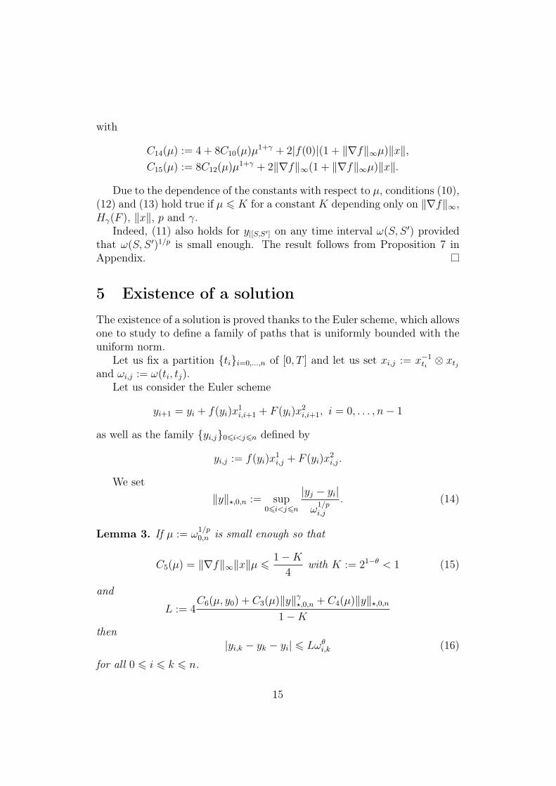
Due to the dependence of the constants with respect to µ, conditions (10),(12) and (13) hold true if µ 6 K for a constant K depending only on ‖∇f‖∞,Hγ(F ), ‖x‖, p and γ.
Indeed, (11) also holds for y|[S,S′] on any time interval ω(S, S ′) providedthat ω(S, S ′)1/p is small enough. The result follows from Proposition 7 inAppendix.
5 Existence of a solutionThe existence of a solution is proved thanks to the Euler scheme, which allowsone to study to define a family of paths that is uniformly bounded with theuniform norm.
Let us fix a partition {ti}i=0,...,n of [0, T ] and let us set xi,j := x−1ti ⊗ xtj
and ωi,j := ω(ti, tj).Let us consider the Euler scheme
yi+1 = yi + f(yi)x1i,i+1 + F (yi)x
2i,i+1, i = 0, . . . , n− 1
as well as the family {yi,j}06i<j6n defined by
yi,j := f(yi)x1i,j + F (yi)x
2i,j.
We set‖y‖?,0,n := sup
06i<j6n
|yj − yi|ω
1/pi,j
. (14)
Lemma 3. If µ := ω1/p0,n is small enough so that
C5(µ) = ‖∇f‖∞‖x‖µ 61−K
4with K := 21−θ < 1 (15)
and
L := 4C6(µ, y0) + C3(µ)‖y‖γ?,0,n + C4(µ)‖y‖?,0,n
1−Kthen
|yi,k − yk − yi| 6 Lωθi,k (16)
for all 0 6 i 6 k 6 n.
15
Proof. The proof of this Lemma follows along the lines the one of Lemma 2.4in [2] and relies on an induction on k − i.
Clearly, (16) is true for k = i+ 1. Fix m > 1 and let us assume that (16)holds for any i < k such that k − i < m.
Let us choose i < k such that k− i = m, m > 2. Let j be the index suchthat ωi,j 6 ωi,k/2 and ωi,j+1 > ωi,k/2. Since ω is super-additive, ωj+1,k 6ωi,k/2 and then
ωθi,j + ωθj+1,k 6 21−θωθi,k = Kωθi,k. (17)
We setyi,j,k := yi,k − yi,j − yj,k.
For j as above, since yj,j+1 − yj − yj+1 = 0, and using (17),
We then face the same estimates as the one in the proof of Lemma 1,where we replace the fact that y is a solution in the sense of Davie with aconstant L by our induction hypothesis on |yi,j − yj + yi|. Then
In addition to (15), we choose µ small enough so that
C8(µ) + 4(1−K)−1µ1+γC3(µ) 61
4(19)
andC9(µ) + 4(1−K)−1µ1+γC3(µ) 6
1
4. (20)
Since γ 6 1, ‖y‖γ?,0,n 6 ‖y‖?,0,n when ‖y‖?,0,n 6 1. Hence,
‖y‖?,0,n 6 max{1, 2C7(µ, y0) + 8µ1+γC6(µ, y0))}.
This proves that for a choice of µ (or equivalently T or n) small enoughdepending only on ‖x‖, ‖∇f‖∞, Hγ(F ), γ and p, then ‖y‖?,0,n is boundedby a constant that depends only on ‖x‖, ‖∇f‖∞, Hγ(F ), γ, p, |f(y0)| and|F (y0)|. However, |F (y0)| and |f(y0)| are bounded by some constants thatdepends only on |f(0)| and ‖∇f‖∞.
The result is proved by finding a sequence n0 = 0 < n1 < · · · < nN suchthat ωn1,ni+1
6 µp with tnN = T and µ satisfying (15), (19) and (20). Sinceω is continuous close to its diagonal, there exists such a finite number N ofintervals, and this number depends only on the choice of µ, and then on ‖x‖,‖∇f‖∞, Hγ(F ), γ and p (and not on y0 nor f(0)). Finally, it is easily shownthat
‖y‖?,0,nN 6 Np−1
N−1∑i=1
‖y‖?,ni,ni+1,
which proves the result by applying the result on the successive time inter-vals [tni , tni+1
] and replacing y0 by yti .
Finally, is order to interpolate the Euler scheme and to get a good control,we shall add an hypothesis on ω, which is trivially satisfied in the case ofω(s, t) = t− s, that is for Hölder continuous rough paths.
17
Hypothesis 3. We assume that there exists a continuous, increasing func-tion ϕ such that
ω(s, t)
ϕ(t)− ϕ(s)and
ϕ(t)− ϕ(s)
ω(s, t)
are bounded for 0 6 s < t 6 T .
Proposition 3. Under Hypotheses 1, 2 and 3, there exists a least a solutionin the sense of Davie to (1).
Proof. From the family {yi}, we construct a path from [0, T ] to Rm by
yt = yi +ϕ(t)− ϕ(ti)
ϕ(ti+1)− ϕ(ti)yi,i+1, t ∈ [ti, ti+1]. (21)
From standard computations, there exists a constant C16 which depends onlyon p and the lower and upper bounds of ω(s, t)/(ϕ(t)− ϕ(s)) such that
‖y‖ 6 C16‖y‖?,0,n.
With Lemma 4, we have a uniform bound in ‖y‖?,0,n, and then on the con-stant L when µ (or n) is small enough. Hence, for any partition satisfyingHypothesis 3, the path y has a p-variation which is bounded by a constantthat does not depend on the choice of the partition.
Now, let yn be a family of paths constructed along an increasing familyof partitions Πn whose meshes decrease to 0.
Then there exists a subsequence {ynk}k>1 of {yn}n∈N∗ which converges inq-variation for q > p to some path y of finite p-variation.
For any (s, t) in ∩n>0Πn,
|yt − ys − f(ys)x1s,t − F (ys)x
2s,t| 6 Lω(s, t)θ.
Since ∩n>0Πn is dense in [0, T ] and y is continuous, this proves that y is thesolution to (16) in the sense of Davie, at least when T is small enough.
The passage from a solution on [0, T ] with T small enough to a globalsolution is done by using the arguments of Lemma 7, Lemma 8 and Propo-sition 6.
6 Distance between two solutions and unique-ness
We now consider a more stringent assumption than Hypothesis 1.
18
Hypothesis 4. The function f is twice continuously differentiable from Rm
to L(Rd,Rm) and is such that∇f , ∇2f are bounded and F (x) := f(x)·∇f(x)is such that ∇F is γ-Hölder continuous with constant Hγ(∇F ) from Rm toL(Rm ⊗ Rd,Rm).
We consider two rough paths u and v of finite p-variation controlled by ω,p ∈ [2, 3), as well as two vector fields f and g satisfying Hypothesis 4. Lety and z be respectively some solutions to yt = y0 +
∫ t0f(ys) dus and zt =
z0 +∫ t
0g(zs) dvs.
We have seen that y and z remain is a ball of radius R that depends onlyon ‖∇f‖∞, ‖∇g‖∞, ‖∇F‖∞, ‖∇G‖∞ (since F and G = g · ∇g are Lipschitzcontinuous), ‖u‖, ‖v‖, y0, z0, |f(0)|, |g(0)|, ω(0, T ), γ and p.
Definition 3. We say that a constant C satisfies Condition (S) if it dependsonly on the above quantities, as well as Hγ(∇F ), Hγ(∇G), ‖∇2f‖∞ and‖∇2g‖∞.
We then set for some functions h, h′,
δR(h, h′) = supz∈B(0,R)
|h(z)− h′(z)|.
We also set
δ(u, v) = ‖u− v‖ and δ(y, z) = sup06s<t6T
|ys,t − zs,t|ω(s, t)1/p
.
Theorem 1. Under Hypotheses 2 and 4, there exists some constant C17
satisfying Condition (S) such that for all (s, t) ∈ ∆2,
The proof of the following corollary is then immediate from the previousestimate.
Corollary 1. Under Hypotheses 2 and 4, there exists a unique solution inthe sense of Davie to (1).
Theorem 1 proves that the Itô map which sends x to the unique solutionto (1) is locally Lipschitz continuous in y0, f and x.
The next lemma is the main estimate of the proof and show why extraregularity shall be assumed on F . This lemma is already well-known (SeeLemma 3.5 in [2]) but we recall its proof which is straightforward.
19
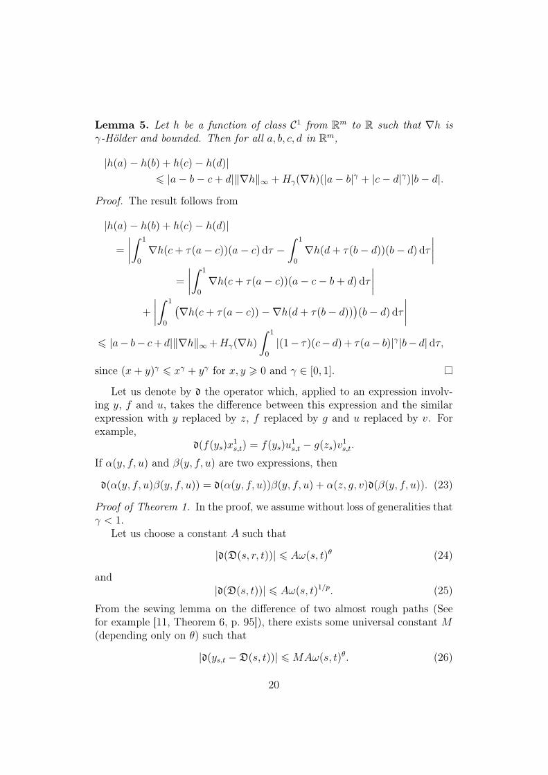
Lemma 5. Let h be a function of class C1 from Rm to R such that ∇h isγ-Hölder and bounded. Then for all a, b, c, d in Rm,
since (x+ y)γ 6 xγ + yγ for x, y > 0 and γ ∈ [0, 1].
Let us denote by d the operator which, applied to an expression involv-ing y, f and u, takes the difference between this expression and the similarexpression with y replaced by z, f replaced by g and u replaced by v. Forexample,
d(f(ys)x1s,t) = f(ys)u
1s,t − g(zs)v
1s,t.
If α(y, f, u) and β(y, f, u) are two expressions, then
Proof of Theorem 1. In the proof, we assume without loss of generalities thatγ < 1.
Let us choose a constant A such that
|d(D(s, r, t))| 6 Aω(s, t)θ (24)
and|d(D(s, t))| 6 Aω(s, t)1/p. (25)
From the sewing lemma on the difference of two almost rough paths (Seefor example [11, Theorem 6, p. 95]), there exists some universal constant M(depending only on θ) such that
|d(ys,t −D(s, t))| 6 MAω(s, t)θ. (26)
20
Our aim is to obtain some estimate on A.Let us note first that
|dF (ys)u2s,t| 6 (|F (ys)− F (zs)|+ |F (zs)−G(zs)|‖u‖ω(s, t)2/p
+ (|G(z0)|+ ‖∇G‖∞‖z‖µ)δ(u, v)ω(s, t)2/p.
Since |ys − zs| 6 δ(y, z)µ+ |y0 − z0|, with Lemma 5,
|F (ys)− F (zs)| 6 ‖∇F‖∞(δ(y, z)µ+ |y0 − z0|),
then for some constant C18 satisfying Condition (S),
and C21 depends only on C19, C20, M and ω(0, T ).Again, choosing µ small enough in function of C19, C20, M and ω(0, T )
gives the required bound in δ(y, z) in short time. As the choice of µ doesnot depend on |y0 − z0| and µ satisfies Condition (S), Proposition 7 may beapplied to y − z.
7 Distance between two Euler schemesLet us give two rough paths u and v of finite p-variations, as well as a partition{ti}ni=0 of [0, T ].
We use the same notations and conventions as in Section 5. Again, weset µ := ω
1/p0,n .
For 0 6 i < j 6 n, we set
zi+1 = zi + g(zi)v1i,i+1 +G(zi)v
2i,i+1, zj = zi + g(zi)v
1i,j +G(zi)v
2i,j,
For a family {εi,j}i,j=1,...,n such that sup06i6j6n |εi,j|/ωθi,j is finite, we set
yi+1 = yi + f(yi)u1i,i+1 + F (yi)u
2i,i+1 + εi,i+1, i = 0, . . . , n− 1 (31)
yj = yi + f(yi)u1i,j + F (yi)u
2i,j + εi,j, 0 6 i < j 6 n.
In addition, define
α := supi=0,...,n−1
|εi,i+1|ωθi,i+1
.
Here, there are three cases of interest: (a) Both z and y are given by someEuler schemes and then εi,j = 0 for all 0 6 i < j 6 n. (b) The path y is asolution to yt = y0 +
∫ t0f(ys) dus and then εi,j = yj−yi−f(yi)u
1i,j−F (yi)u
2i,j,
while v = u and g = f . (c) While v = u and g = f , the family {yi}i=0,...,n isgiven by the Euler scheme with respect to a partition {t′i}i=0,...,m ⊂ {ti}i=0,...,n.
We assume that z and y belong to the ball of radius R and that ‖z‖?,0,nand ‖y‖?,0,n (defined by (14)) are bounded by R′. In any cases, R and R′
depend only on ‖∇f‖∞, ‖∇F‖∞, ‖∇g‖∞, ‖∇G‖∞, ‖u‖, ‖v‖, |f(0)|, |g(0)|,|y0|, |z0|, ω(0, T ), γ and p.
23
Definition 4. We say that a constant C satisfies condition (Se) if it dependsonly on the quantities listed above as well as Hγ(∇F ), Hγ(∇G), ‖∇2f‖∞,‖∇2g‖∞ and sup06i6j6n |εi,j|/ωθi,j.
Theorem 2. If f and g satisfies Hypothesis 4, then for some constant C22
On the other hand, since both f and F are Lipschitz continuous, for someconstant C25 satisfying Condition (Se),
‖z − y‖?,0,n 6 sup06i<j6n
|yj − yi − yi,j − zj + zi + zi,j|ω
1/pi,j
+|yi,j − zi,j|
ω1/pi,j
6 Aµ1+γ + C25(|y0 − z0|+ µ‖z − y‖?,0,n) +B2
withB2 := C26(δR(F,G) + δR(f, g) + δ(u, v)),
for some constant C26 satisfying Condition (Se). If µ is small enough so thatC25µ 6 1/2, then
‖z − y‖?,0,n 6 2C25|y0 − z0|+ 2Aµ1+γ + 2B2. (34)
Injecting this in (33),
A 6 2α +KA+ C27(|y0 − z0|+ AC28(µ)) +B3
with a C28(µ) satisfying Condition (Se) for fixed µ and that decreases to 0 as µdecreases to 0, C27 satisfying Condition (Se), and B3 = C29(B1+B2) for someconstant C29 satisfying Condition (Se). For K +C27C28(µ) < (1 +K)/2 < 1,then
A 62
1−K(2α + C27|y0 − z0|+B3).
Using the inequality on (34), this leads to the required inequality for a valueof µ small enough. Thus usual arguments proves now that this is true forany time horizon T up to changing the constants.
25
8 Rate of convergence of the Euler scheme
Let us consider now the solution to yt = y0 +∫ t
0f(ys) dxs as well as the
associated Euler scheme
ei+1 = ei + f(ei)x1i,i+1 + F (ei)x
2i,i+1, e0 = y0
when f satisfies Hypothesis 4.We are willing to estimate the difference between y and e. Our key
argument is provided by Theorem 2 above.
Proposition 4. Assume Hypothesis 4 on f . For δ := sup06i<n ωi,i+1 andp ∈ [2, 3),
supi=0,...,n
|ei − yi| 6 C30δ(3−p)/p−η. (35)
where C30 depends only on y0, |f(0)|, ‖x‖, ‖∇f‖∞, ‖∇2f‖∞, ‖∇F‖∞, Hγ(∇F ),ω(0, T ), p and γ.
It follows that the rate of convergence is smaller than (3 − p)/p andbelongs to (0, 1/2). In addition, when p increases to 3, the rate of convergencedecreases to 0. This rate is similar to the one given by A.M. Davie [2]. (Seealso [3] for the convergence of the Milstein scheme for the fractional Brownianmotion).
Proof. Let us note first that since y and e remains bounded, if ∇F is γ-Hölder continuous, then it is locally γ′-Hölder continuous for any γ′ < γ.Since the constraint 2 + γ′ > p is in force, we set γ′ = p − 2 + ηp for some0 < η < (3− p)/p < 1/2 and θ′ := (2 + γ′)/p = 1 + η.
Since F is Lipschitz continuous, then y is a solution in the sense of Daviewith θ = 3/p. This way,
|yt − ys − f(ys)x1s,t − F (ys)x
2s,t| 6 Lω(s, t)3/p.
It follows that {yi}ni=0 is solution to (31) with
εi,i+1 = yi+1 − yi − f(yi)x1i,i+1 − F (yi)x
2i,i+1.
Thenα := sup
06i<n
|εi,i+1|ωθ′i,i+1
6 Lδ3/p−θ′ = Lδ(3−p)/p−η.
Applying Theorem 2 with our choice of θ′ leads to
‖e− y‖ 6 C31δ(3−p)/p−η,
where C31 depends only on y0, |f(y0)|, ‖x‖, ‖∇f‖∞, ‖∇2f‖∞, ‖∇F‖∞,Hγ(∇F ), ω(0, T ), p and γ. Then (35) is immediate.
26
Let {{tni }i=0,...,n}n∈N∗ be an increasing family of partitions such that themesh supi=0,...,n ω(tni , t
ni+1) converges to 0. Let {{eni }i=0,...,n}n∈N∗ be the cor-
responding Euler schemes for a rough path x and a vector field f satisfiesHypothesis 4. With Lemmas 3, 4 and 8,
supn∈N∗
sup06i<j6n
|eni − enj − f(eni )x1tni ,tj− F (eni )x2
tni ,tnj|
ω(tni , tnj+1)θ
< +∞
and with Proposition 3 under Hypothesis 3, the interpolation of the Eu-ler scheme en constructed as in (21) has a p-variation norm ‖en‖ which isbounded. Using the same proof as above, we get the following corollary.
Corollary 2. Under Hypotheses 2, 3 and 4, the family of interpolated Eulerschemes {en}n∈N∗ for a Cauchy sequence of the uniform norm and the q-variation norm for any q > p.
Remark 2. Here the dimension d of the space plays no role so that thisargument may be used for an infinite dimensional rough path. This Corollaryallows one to define the solution to (1) as the limit of the sequence {en}n∈N∗ .
9 Case of geometric rough pathsWe now consider the case where x is a geometric rough path of finite p-variation controlled by ω and the vector field f satisfies Hypothesis 4. Thismeans that there exists a sequence of rough paths xn converging to x inp-variation such that xn lives above a piecewise smooth path zn in Rd andxnt = 1 + znt +
∫ t0(zns − zn0 )⊗ zns ds. Such a path xn is called a smooth rough
path.In order to simplify the analysis, we assume that ω(s, t) = t− s and then
we are dealing with α-Hölder continuous paths with α = 1/p.The core idea of P. Friz and N. Victoir was to consider a family of smooth
rough paths (xn)n>1 such that, given a family of partitions {{tni }i=0,...,n}n∈N∗ ,xn converges to x in the β-Hölder norm for any β < α and xntni = xtni for i =0, . . . , n.
For this, they used sub-Riemannian geodesics. In [11], we have providedan alternative construction using some segments and some loops.
Let zn be the projection of xn onto Rd, and let yn be the solution ofthe ODE ynt = y0 +
∫ t0f(yns ) dzns . As zn is piecewise smooth, one knows
that this solution corresponds to the one of the solution of the RDE ynt =y0+
∫ t0f(yns ) dxns in the sense of Davie or in the sense of Lyons (See Section 10
below).
27
Let en be the Euler scheme associated to yn with the partition {tni }i=0,...,n:
eni+1 = eni + f(eni )x1,ntni ,t
ni+1
+ F (eni )x2,ntni ,t
ni+1, i = 0, . . . , n,
and en the Euler scheme
eni+1 = eni + f(eni )x1,ntni ,t
ni+1
+ F (eni )x2,ntni ,t
ni+1, i = 0, . . . , n,
The key observation from P. Friz and N. Victoir is that from the veryconstruction of xn, xntni ,tni+1
= xntni ,tni+1and then en = en.
With Proposition 4, for some η ∈ (0, 3α− 1),
‖en − yn‖? := sup06i<j6n
|enj − eni − ynj + yni |ω
1/pi,j
= ‖en − yn‖ 6 C32δ3α−1−η
where C32 depends only on ‖x‖, f , T , α and η, and δ := supi=0,...,n+1 ω(tni , tni+1).
On the other hand with Theorem 1,
‖yn − ym‖? 6 ‖yn − ym‖ 6 C33‖xm − xn‖,
where C33 depends only on ‖x‖, f , T , α and η (when xn is such that ‖xn‖ 6A‖x‖ which is the case with the constructions mentioned above).
Since (xn)n∈N∗ is a Cauchy sequence in the space of β-Hölder continuousfunctions, β < α, it follows that (yn) is a Cauchy sequence and converges tosome element y.
We then obtain the convergence of en to y in the sense that ‖en − y‖?decreases to 0 as n tends to infinity.
10 Solution in the sense of Davie and solutionin the sense of Lyons
The notion of solution in the sense of Davie (Definition 2) is different of thesolution in the sense of Lyons (Definition 1), as the iterated integrals of yand the cross-iterated integrals between y and x are not constructed, whilethey are part of the solution in the sense of Lyons.
However, once a solution in the sense of Davie is constructed, it is easyto construct a rough paths with values in T1(Rd ⊕ Rm).
Lemma 6. A solution y in the sense of Davie — which is a path with valuesin Rm — may be lifted to a rough path with values in T1(Rd ⊕ Rm), as therough path y associated to the almost rough path
Besides, the map y 7→ y is locally Lipschitz continuous.
28
Proof. It is easily checked that
|hs,r,t − hs,r ⊗ hr,t| 6 C34ω(s, t)θ
with θ > 1 and then that it is an almost rough path. With Proposition 1, theassociated rough path y projects onto (x, y) in Rd⊕Rm. The local Lipschitzcontinuity of y 7→ y follows from the same kind of computation as the one ofthe proof of Theorem 1.
Proposition 5. Let us assume that f is a vector field with a bounded deriva-tive which is γ-Hölder continuous, such that a solution to (1) exists in thesense of Lyons. Let us assume also that f · ∇f is γ-Hölder continuous, sothat a solution to (1) exists in the sense of Davie, lifted as a rough path withvalues in T1(Rd ⊕ Rm) as above. Then the two solutions coincide.
Proof. Let y be a solution in the sense of Davie of (1), which is lifted as arough path y using Lemma 6. Let us consider
us,t := f(ys)x1s,t +∇f(ys)y
×s,t,
where y×s,t is the projection onto Rm ⊗ Rd of ys,t (or roughly speaking, it isthe cross-iterated integral between y and x).
Then {us,t}(s,t)∈∆2 is an almost rough path in Rm whose associated roughpath v satisfies
|vt − vs − us,t| 6 C35ω(s, t)θ.
From the very construction, v is the rough integral vt = v0 +∫ t
0g(zs) dzs with
z is a rough path lying above (x, y, y×) ∈ (R ⊕ Rd ⊕ Rd,Rm,Rm ⊗ Rd) andg(y, x) = dx + f(y) dx. Thus y = v when v0 = y0. With Lemma 6, thisis also true for the iterated integrals. This proves that the a solution in thesense of Davie is also a solution in the sense of Lyons.
If z is a solution in the sense of Lyons, by construction, for a constant Land all (s, t) ∈ ∆2,
|zt − zs − f(zs)x1s,t −∇f(zs)z
×s,t| 6 Lω(s, t)θ
and |z×s,t 6 1⊗ f(zs)x2s,t| 6 Lω(s, t)θ,
29
where z× lives in Rm⊗Rd. Hence, it is immediate the a solution in the senseof Lyons is also a solution in the sense of Davie.
A From local to global theoremsWe present here some results which allows one to pass from local estimatesto global estimates and then show the existence for any horizon T providedsome uniform estimates.
Lemma 7. Let µ > 0 be fixed. Then there exists a finite number of times0 = T0 < T1 < · · · < TN+1 with TN 6 T < TN+1 and ω(Ti, Ti+1) = µ.
Proof. Let us extend ω on D+ := {(s, t) | 0 6 s 6 t} by
ω(s, t) =
{ω(s, T ) + T − s if s 6 T 6 t,
t− s if T 6 s 6 t.
Let us note that ω is continuous on D+, and that ω(s, t) −−−→t→∞
+∞. Then forany µ > 0, for any s > 0, there exists a value τ(s) such that ω(s, τ(s)) = µ,since ω(s, s) = 0.
For T > 0 fixed, let us set T0 = 0 and Ti+1 = τ(Ti). Then there ex-ists a finite number N such that ω(0, TN−1) 6 ω(0, T ) 6 ω(T0, TN+1) andω(Ti, Ti+1) = µ. This follows from the fact that
Nµ =N−1∑i=0
ω(Ti, Ti+1) 6 ω(0, TN)
and then ω(0, TN) −−−→N→∞
+∞. This proves the lemma.
For a path y and times 0 6 S < S ′ 6 T , let us set
‖y‖[S,S′] := supS6s<t6S′
|yt − ys|ω(s, t)1/p
.
Lemma 8. Let us assume that a continuous path y on [S, S ′′] is a solutionin the sense of Davie on time interval [S, S ′] and [S ′, S ′′] respectively withconstants L1 and L2. Then y is a solution in the sense of Davie on [S, S ′′]with a new constant L3 that depends only on L1, L2, Hγ(F ), ‖∇f‖∞, ‖x‖,‖y‖|[S,S′], ω(0, T ), γ and p.
30
Proof. First, it is classical that
‖y‖[S,S′′] 6 21−1/p max{‖y‖[S,S′], ‖y‖[S′,S′′]},
so that y is of finite p-variation over [S, S ′′]. For s ∈ [S, S ′] and t ∈ [S ′, S ′′],
where C36 depends only on L1, ‖y‖|[S,S′],Hγ(F ), ‖∇f‖∞, |F (ys)|, ‖x‖, ω(0, T ),γ and p. Hence, since ω(s, S ′)θ + ω(S ′, t) 6 ω(s, t),
|yt − ys −D(s, t)| 6 (max{L1, L2}+ C36)ω(s, t)θ.
This proves the result.
Proposition 6. Let us assume that a solution to (1) exists on any timeinterval [S, S ′] with a condition that ω(S, S ′) 6 C37 where C37 does not dependon S. Then a solution exists for any time T .
Proof. Using the sequence {Ti}i=0,...,N of times given by Lemma 7, it is suf-ficient to solve (1) successively on [Ti, Ti+1] with initial condition yTi and toinvoke Lemma 8 to prove the existence of a solution in the sense of Daviein [0, T ].
Proposition 7. Let y be a path of finite p-variations such that for someconstants A, B and K,
when ω(S, S ′) 6 K, ‖y‖[S,S′] 6 B|yS|+ A.
Thensupt∈[0,T ]
|yt| 6 R(T )|y0|+ (R(T )− 1)A
B(37)
withR(T ) = exp(B(1 +K−1)1−1/p max{ω(0, T ), ω(0, T )1/p}),
and the p-variation norm of ‖y‖[0,T ] depends only on A, B, ω(0, T ), K and p.
Proof. Remark first that
supt∈[S,S′]
|yt| 6 |yS|(1 +Bω(S, S ′)1/p) + Aω(S, S ′)1/p.
31
Let us choose an integer N such that µ := ω(0, T )/N 6 K and constructrecursively Ti with T0 = 0 and ω(Ti, Ti+1) = µ. Then
|yTi+1| 6 |yTi |(1 + µ1/pB) + Aµ1/p.
From a classical result easily proved by an induction,
|yT | 6 exp(Nµ1/pB)|y0|+A
B(exp(Nµ1/pB)− 1).
As this is true for any T , surely (37) holds.Choosing N such that ω(0, T )/N 6 K and ω(0, T )/(N − 1) > K,
N 6ω(0, T )
K+ 1.
This way
Nµ1/p 6
(ω(0, T )
K+ 1
)1− 1p
ω(0, T )1p 6
{Kω(0, T )1/p if ω(0, T ) 6 1,
Kω(0, T ) if ω(0, T ) > 1.
with K := (1 +K−1)1−1/p.Finally,
‖y‖[0,T ] 6 N1−1/p maxi=0,...,N−1
‖y‖[Ti,Ti+1],
which proves the last statement
References[1] S. Aida, Notes on proofs of continuity theorem in rough path analysis (2006). Preprint
of Osaka University.
[2] A.M. Davie, Differential Equations Driven by Rough Paths: an Approach via DiscreteApproximation, Appl. Math. Res. Express. AMRX 2 (2007), Art. ID abm009, 40.
[3] A. Deya, A. Neuenkirch, and S. Tindel, A Milstein-type scheme without Levy areaterms for SDEs driven by fractional Brownian motion (2010). arxiv:1001.3344.
[4] H. Doss, Liens entre équations différentielles stochastiques et ordinaires, Ann. Inst.H. Poincaré Sect. B (N.S.) 13 (1977), no. 2, 99–125.
[5] P. Friz and N. Victoir, Euler Estimates of Rough Differential Equations, J. DifferentialEquations 244 (2008), no. 2, 388–412.
[6] , Multidimensional Stochastic Processes as Rough Paths. Theory and Applica-tions, Cambridge University Press, 2010.
32
[7] J. G. Gaines and T. J. Lyons, Variable step size control in the numerical solution ofstochastic differential equations, SIAM J. Appl. Math. 57 (1997), no. 5, 1455–1484,DOI 10.1137/S0036139995286515.
[8] M. Gubinelli, Controlling rough paths, J. Funct. Anal. 216 (2004), no. 1, 86–140.
[9] Y. Inahama and H. Kawabi, Asymptotic expansions for the Laplace approximationsfor Itô functionals of Brownian rough paths, J. Funct. Anal. 243 (2007), no. 1, 270–322.
[10] A. Lejay, An introduction to rough paths, Séminaire de probabilités XXXVII, LectureNotes in Mathematics, vol. 1832, Springer-Verlag, 2003, pp. 1–59.
[11] , Yet another introduction to rough paths, Séminaire de probabilités XLII,Lecture Notes in Mathematics, vol. 1979, Springer-Verlag, 2009, pp. 1–101.
[12] , On rough differential equations, Electron. J. Probab. 14 (2009), no. 12, 341–364.
[13] , Controlled differential equations as Young integrals: a simple approach, J.Differential Equations 249, 1777-1798, DOI 10.1016/j.jde.2010.05.006.
[14] A. Lejay and N. Victoir, On (p, q)-rough paths, J. Differential Equations 225 (2006),no. 1, 103–133.
[15] T.J. Lyons, Differential equations driven by rough signals, Rev. Mat. Iberoamericana14 (1998), no. 2, 215–310.
[16] T. Lyons and Z. Qian, Flow of diffeomorphisms induced by a geometric multiplicativefunctional, Probab. Theory Related Fields 112 (1998), no. 1, 91–119.
[17] , System Control and Rough Paths, Oxford Mathematical Monographs, OxfordUniversity Press, 2002.
[18] T. Lyons, M. Caruana, and T. Lévy, Differential Equations Driven by Rough Paths,École d’été des probabilités de Saint-Flour XXXIV — 2004 (J. Picard, ed.), LectureNotes in Mathematics, vol. 1908, Springer, 2007.
[19] D. S. Mitrinović, J. E. Pečarić, and A. M. Fink, Inequalities involving functions andtheir integrals and derivatives, Mathematics and its Applications (East EuropeanSeries), vol. 53, Kluwer Academic Publishers Group, 1991.
[20] H.J. Sussmann, On the gap between deterministic and stochastic ordinary differentialequations, Ann. Probability 6 (1978), no. 1, 19–41.