The Blasius equation - HAL - INRIA

HAL Id: hal-00765316https://hal.archives-ouvertes.fr/hal-00765316

Submitted on 14 Dec 2012

HAL is a multi-disciplinary open accessarchive for the deposit and dissemination of sci-entific research documents, whether they are pub-lished or not. The documents may come fromteaching and research institutions in France orabroad, or from public or private research centers.

L’archive ouverte pluridisciplinaire HAL, estdestinée au dépôt et à la diffusion de documentsscientifiques de niveau recherche, publiés ou non,émanant des établissements d’enseignement et derecherche français ou étrangers, des laboratoirespublics ou privés.

The Blasius equationB. Brighi, A. Fruchard, T. Sari

To cite this version:B. Brighi, A. Fruchard, T. Sari. The Blasius equation. Colloque à la mémoire d’Emmanuel Isambert,Université de Paris 7, Dec 2007, Paris, France. Publications de l’Université de Paris 13, p. 105 - p.123, 2012. <hal-00765316>

https://hal.archives-ouvertes.fr/hal-00765316

https://hal.archives-ouvertes.fr

The Blasius equation

Bernard Brighi, Augustin Fruchard, Tewfik Sari

Abstract. The Blasius problem f ′′′ + ff ′′ = 0, f(0) = −a, f ′(0) = b, f ′(+∞) = λ is investigated,in particular in the difficult and scarcely studied case b < 0 � λ. The shape and the number ofsolutions are determined. The method is first to reduce to the Crocco equation uu′′ + s = 0 andthen to use an associated autonomous planar vector field. The most useful properties of Croccosolutions appear to be related to canard solutions of a slow fast vector field.

Keywords : Blasius equation, Crocco equation, boundary value problem on infinite interval, canardsolution.

1 Introduction

In this article we present a selection of results of [6]. The reader is referred to [6] for completeproofs, additional and intermediate results. We take the occasion to completely change the orderof presentation: in [6] we first give the results on the Blasius equation with a sketch of proof,then we introduce the Crocco equation and the vector field, we establish results and proofs onthese intermediate equations and then we return to the proof of the initial result. Here we choosea different order and we postpone the main result at the end of the article. We hope that thisarticle may be a first approach before a thorough study of [6].

The article is organized as follows. In Section 2, we state the main problem of the paperwhich is the investigation of the following Blasius Boundary Value Problem (BBVP for short)

f ′′′ + ff ′′ = 0 on [0, +∞[, (1)

f(0) = −a, f ′(0) = b, limt→+∞

f ′(t) = λ. (2)

We list some former results, according to the relative values of b and λ, and we focus ourattention on the case b < 0 � λ, which is our case of interest. In Section 3, we show that, in thelatter case, this boundary value problem is equivalent to the Crocco Boundary Value Problem(CBVP) ⎧⎨

⎩uu′′ + s = 0 on [b, λ[,

u′(b) = a, lims→λ

u(s) = 0.(3)

where [b, λ[ appears as the maximal right-interval of definition of the solution. In Section 4, weshow that the similarity properties of the Blasius or the Crocco solutions permit to reduce thenon autonomous second order differential equation of Crocco to an autonomous planar vectorand we notice that the maximal right-interval of definition of the solutions of the Crocco equationpresents a discontinuity with respect to the initial condition. It is well known that the maximalright-interval of definition of the solution of a differential equation is not continuous in generalwith respect to the initial conditions. It is simply lower semicontinuous. Actually, in Section 6,we see that the solutions of the Crocco differential equation which are close to 0 for s close to0 are canard solutions of a slow-fast vector field. These solutions play an important role in the

105

The original publication is available at http://hal.archives-ouvertes.fr/hal-00493860/

Colloque à la mémoire d’Emmanuel Isambert, Université de Paris 7, 21-22 décembre 2007

106 B. Brighi, A. Fruchard, T. Sari

description of the discontinuity of the maximal right-interval of definition of the solution of theCrocco equation. In Section 7, we analyze this discontinuity which occurs along a particularorbit of the planar vector field considered in Section 4. In Section 8, we give a lower boundof the number of solutions of the boundary value problem associated to the Blasius equation,in the case b < 0 � λ. Section 9 describes a difficulty encountered in numerical simulations.Indeed, due to the canard solutions phenomenon, some solutions of the Crocco equation becomeexponentially small for s < 0 and the numerical scheme cannot give the right solution. We showhow to use the theoretical study in Section 5 to overcome this difficulty.

2 The Blasius Boundary Value Problem

The Blasius Boundary Value Problem (1-2) arises for the first time, with a = b = 0 and λ = 2,in 1907 in the thesis of Blasius [3, 4]. In the case a = b = 0, Hermann Weyl [16] proves thatthe BBVP has one and only one solution. The proof is elementary but strongly uses the factthat a = b = 0, see also [5, 8]. The BBVP plays a central role in fluid mechanics [12]: TheBlasius equation (1) was obtained using a similarity transform and enabled successful treatmentof the laminar boundary layer on a flat plate. By considering equation (1) as a first order lineardifferential equation for f ′′, we obtain

f ′′(t) = f ′′(0) exp

{−

∫ t

0f(τ)dτ

}.

Hence, the BBVP splits into three cases, called respectively linear, concave and convex:

• If λ = b, then the BBVP has a unique solution, given by f(t) = bt − a.

• If λ > b, then any possible solution must satisfy f ′′(t) > 0 for all t � 0, i.e. has to beconvex.

• If λ < b, then possible solutions are concave.

The concave case is completely solved and well-known [1].

Proposition 1 — In the case λ < b, the BBVP (1 - 2) has exactly one solution if 0 � λ < b,and no solution if λ < 0.

When b � 0, the convex case λ > b is also well-known, see [8].

Proposition 2 ([6] Corollary 3.6) — The BBVP (1 - 2), where b � 0 and λ > b, has exactlyone solution when a � 0 or b > 0. When a > 0 and b = 0, the BBVP has exactly one solutionfor all λ > a2λ+ and no solution if 0 < λ � a2λ+, where λ+ � 1.304 is defined in Proposition 5.

It is known that every solution of the Blasius equation (1) such that f ′′(0) > 0 is defined for allt and its derivative has a finite and non-negative limit as t → +∞ ([6] Proposition 3.1). Thus

Proposition 3 — The BBVP (1 - 2) has no solution if b < λ < 0.

In this article, we focus on the remaining case b < 0 � λ, which is much richer and trickier. Nonuniqueness for the BBVP is mentioned in the literature, but either only supported by numericalinvestigations [9], or with incomplete proofs [10, 13].

The Blasius equation (1) has the following similarity property:

If t �→ f(t) is a solution of (1), so is t �→ σf(σt), for all σ ∈ R. (4)



The Blasius equation 107

b

λ

a2λ+−

linear

linear

convex

concave

0

0

0

1

1

1

11

1

0

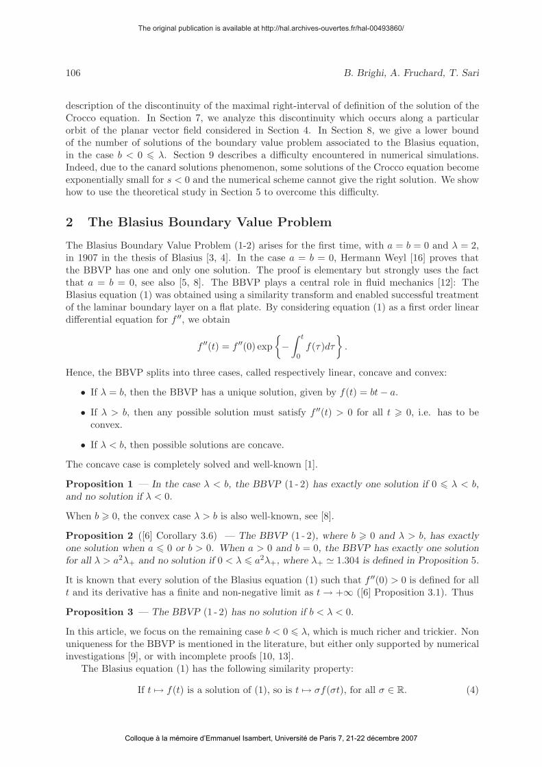
Figure 1: In the plane (b, λ), the number of solutions of the BBVP (5) in each region and ontheir border. In gray, the remaining region to investigate, purpose of this article.

This allows us to restrict our attention without loss of generality to the case b = −1, i.e. to theBBVP ⎧⎨

⎩f ′′′ + ff ′′ = 0 on [0, +∞[,

f(0) = −a, f ′(0) = −1, limt→+∞

f ′(t) = λ � 0.(5)

The purpose of this article is to count the number of solutions of (5). The main result, at theend of Section 8, gives a minimum number of solutions of (5) depending on the values of a andλ. We conjecture that this minimum number is the exact number of solutions.

3 The Crocco Boundary Value Problem

Let f be a convex solution of (1). Since f ′′ > 0 it follows that t �→ f ′(t) is a diffeomorphism.Hence we can use f ′ as an independent variable and express f ′′ as a function of f ′. This is theso-called Crocco transformation [7]

s = f ′, f ′′ = u(s)

Differentiating f ′′ = u(f ′) we obtain u′(s) = −f . Differentiating once again we obtain that usatisfies the following so-called Crocco differential equation

u′′u + s = 0. (6)

As we will see, the BBVP (5) is equivalent to the Crocco Boundary Value Problem (3) forb = −1, rewritten below for convenience⎧⎨

⎩uu′′ + s = 0 on [−1, λ[,

u′(−1) = a, lims→λ

u(s) = 0.(7)

The equivalence between (5) and (7) will become clear after the following remarks. In order tosolve (5) we use the shooting method. Let f( · ; a, c) denote the solution of the Blasius Initial




0

2

4

6

8

10

5 10

0

0.5

1

–1 1

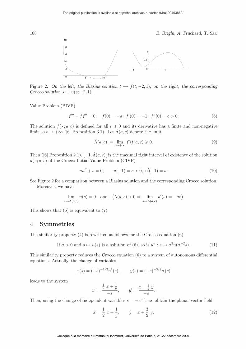
Figure 2: On the left, the Blasius solution t �→ f(t;−2, 1); on the right, the correspondingCrocco solution s �→ u(s;−2, 1).

Value Problem (BIVP)

f ′′′ + ff ′′ = 0, f(0) = −a, f ′(0) = −1, f ′′(0) = c > 0. (8)

The solution f( · ; a, c) is defined for all t � 0 and its derivative has a finite and non-negativelimit as t → +∞ ([6] Proposition 3.1). Let Λ(a, c) denote the limit

Λ(a, c) := limt→+∞

f ′(t; a, c) � 0. (9)

Then ([6] Proposition 2.1), [−1, Λ(a, c)[ is the maximal right interval of existence of the solutionu( · ; a, c) of the Crocco Initial Value Problem (CIVP)

uu′′ + s = 0, u(−1) = c > 0, u′(−1) = a. (10)

See Figure 2 for a comparison between a Blasius solution and the corresponding Crocco solution.Moreover, we have

lims→eΛ(a,c)

u(s) = 0 and(Λ(a, c) > 0 ⇒ lim

s→eΛ(a,c)u′(s) = −∞)

This shows that (5) is equivalent to (7).

4 Symmetries

The similarity property (4) is rewritten as follows for the Crocco equation (6)

If σ > 0 and s �→ u(s) is a solution of (6), so is uσ : s �→ σ3u(σ−2s). (11)

This similarity property reduces the Crocco equation (6) to a system of autonomous differentialequations. Actually, the change of variables

x(s) = (−s)−1/2u′ (s) , y(s) = (−s)−3/2u (s)

leads to the system

x′ =

12 x + 1

y

−s, y′ =

x + 32 y

−s.

Then, using the change of independent variables s = −e−τ , we obtain the planar vector field

x =1

2x +

1

y, y = x +

3

2y, (12)




Γ∞

S∗

�x

�y

��y = R1(x)

xy = −2

��y = L1(x)

��y = R2(x)

Γ∞

S∗

�xa2 a3 a1

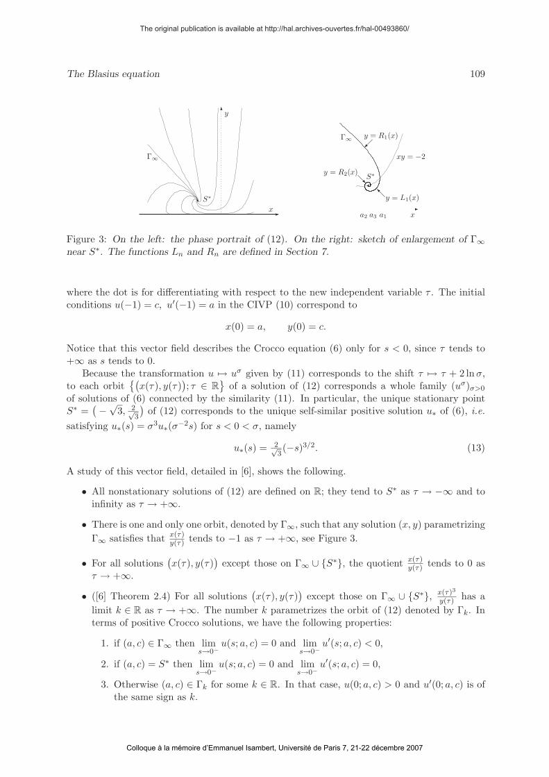
Figure 3: On the left: the phase portrait of (12). On the right: sketch of enlargement of Γ∞near S∗. The functions Ln and Rn are defined in Section 7.

where the dot is for differentiating with respect to the new independent variable τ . The initialconditions u(−1) = c, u′(−1) = a in the CIVP (10) correspond to

x(0) = a, y(0) = c.

Notice that this vector field describes the Crocco equation (6) only for s < 0, since τ tends to+∞ as s tends to 0.

Because the transformation u �→ uσ given by (11) corresponds to the shift τ �→ τ + 2 lnσ,to each orbit

{(x(τ), y(τ)

); τ ∈ R

}of a solution of (12) corresponds a whole family (uσ)σ>0

of solutions of (6) connected by the similarity (11). In particular, the unique stationary pointS∗ =

( −√3, 2√

3

)of (12) corresponds to the unique self-similar positive solution u∗ of (6), i.e.

satisfying u∗(s) = σ3u∗(σ−2s) for s < 0 < σ, namely

u∗(s) = 2√3(−s)3/2. (13)

A study of this vector field, detailed in [6], shows the following.

• All nonstationary solutions of (12) are defined on R; they tend to S∗ as τ → −∞ and toinfinity as τ → +∞.

• There is one and only one orbit, denoted by Γ∞, such that any solution (x, y) parametrizing

Γ∞ satisfies that x(τ)y(τ) tends to −1 as τ → +∞, see Figure 3.

• For all solutions(x(τ), y(τ)

)except those on Γ∞ ∪ {S∗}, the quotient x(τ)

y(τ) tends to 0 asτ → +∞.

• ([6] Theorem 2.4) For all solutions(x(τ), y(τ)

)except those on Γ∞ ∪ {S∗}, x(τ)3

y(τ) has a

limit k ∈ R as τ → +∞. The number k parametrizes the orbit of (12) denoted by Γk. Interms of positive Crocco solutions, we have the following properties:

1. if (a, c) ∈ Γ∞ then lims→0−

u(s; a, c) = 0 and lims→0−

u′(s; a, c) < 0,

2. if (a, c) = S∗ then lims→0−

u(s; a, c) = 0 and lims→0−

u′(s; a, c) = 0,

3. Otherwise (a, c) ∈ Γk for some k ∈ R. In that case, u(0; a, c) > 0 and u′(0; a, c) is ofthe same sign as k.




0.5

1

1.5

–1 –0.5

0.5

1

1.5

–1 –0.5 0.5 1 1.5 2

��

�

��

�

��

��

��

��

� ��

��

��

� ��

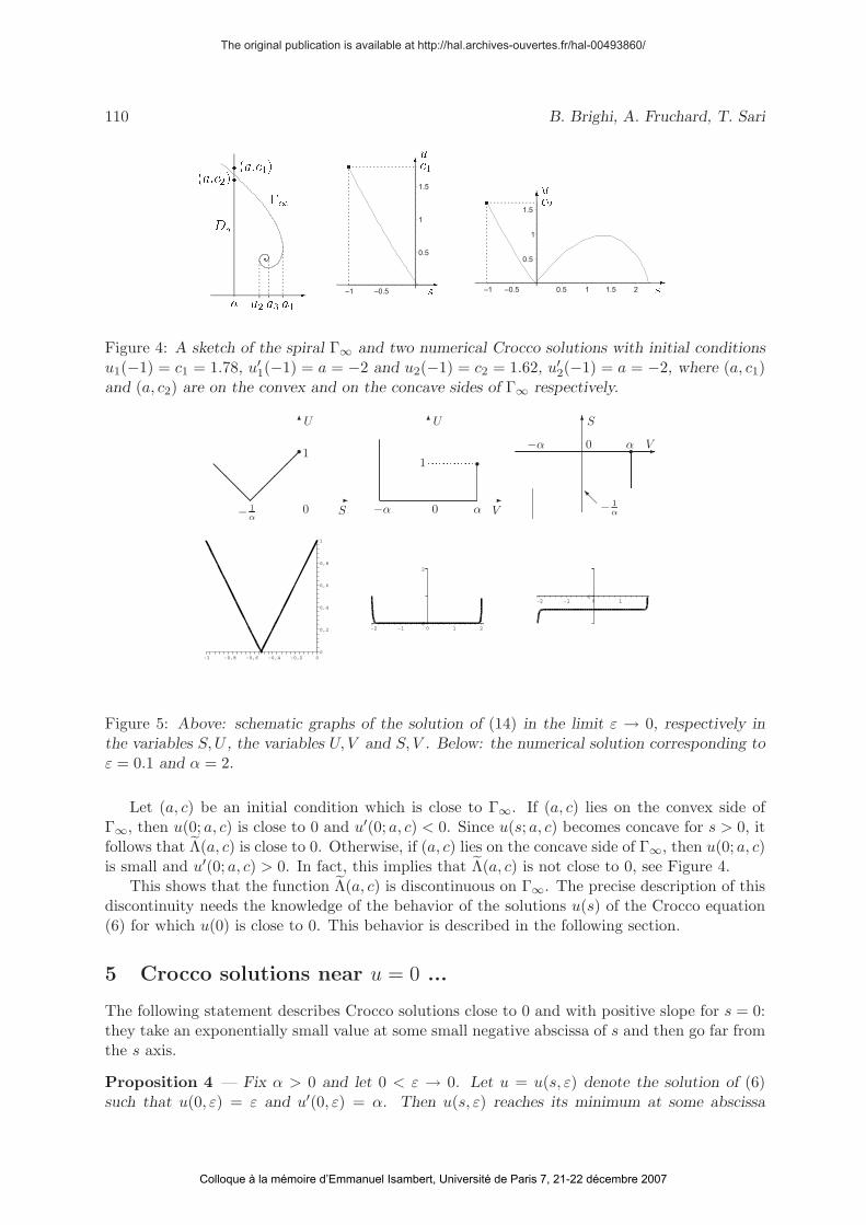
Figure 4: A sketch of the spiral Γ∞ and two numerical Crocco solutions with initial conditionsu1(−1) = c1 = 1.78, u′

1(−1) = a = −2 and u2(−1) = c2 = 1.62, u′2(−1) = a = −2, where (a, c1)

and (a, c2) are on the convex and on the concave sides of Γ∞ respectively.

�− 1

α

0 S

�

1

U

��

��

��

�

�−α 0 α V

�U

1 �

�−α 0 α V

�S

�� − 1

α

�

0,4

-0,4

0,2

0-0,6-0,8-1

1

0

0,8

-0,2

0,6

210-1-2

2

0

210-1-20

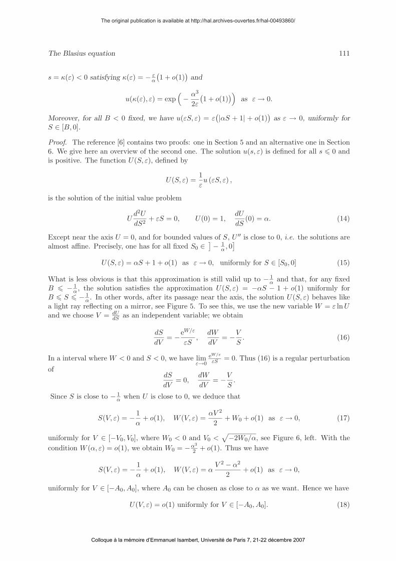
Figure 5: Above: schematic graphs of the solution of (14) in the limit ε → 0, respectively inthe variables S, U , the variables U, V and S, V . Below: the numerical solution corresponding toε = 0.1 and α = 2.

Let (a, c) be an initial condition which is close to Γ∞. If (a, c) lies on the convex side ofΓ∞, then u(0; a, c) is close to 0 and u′(0; a, c) < 0. Since u(s; a, c) becomes concave for s > 0, itfollows that Λ(a, c) is close to 0. Otherwise, if (a, c) lies on the concave side of Γ∞, then u(0; a, c)is small and u′(0; a, c) > 0. In fact, this implies that Λ(a, c) is not close to 0, see Figure 4.

This shows that the function Λ(a, c) is discontinuous on Γ∞. The precise description of thisdiscontinuity needs the knowledge of the behavior of the solutions u(s) of the Crocco equation(6) for which u(0) is close to 0. This behavior is described in the following section.

5 Crocco solutions near u = 0 ...

The following statement describes Crocco solutions close to 0 and with positive slope for s = 0:they take an exponentially small value at some small negative abscissa of s and then go far fromthe s axis.

Proposition 4 — Fix α > 0 and let 0 < ε → 0. Let u = u(s, ε) denote the solution of (6)such that u(0, ε) = ε and u′(0, ε) = α. Then u(s, ε) reaches its minimum at some abscissa




s = κ(ε) < 0 satisfying κ(ε) = − εα

(1 + o(1)

)and

u(κ(ε), ε) = exp(− α3

2ε

(1 + o(1)

))as ε → 0.

Moreover, for all B < 0 fixed, we have u(εS, ε) = ε(|αS + 1| + o(1)

)as ε → 0, uniformly for

S ∈ [B, 0].

Proof. The reference [6] contains two proofs: one in Section 5 and an alternative one in Section6. We give here an overview of the second one. The solution u(s, ε) is defined for all s � 0 andis positive. The function U(S, ε), defined by

U(S, ε) =1

εu (εS, ε) ,

is the solution of the initial value problem

Ud2U

dS2+ εS = 0, U(0) = 1,

dU

dS(0) = α. (14)

Except near the axis U = 0, and for bounded values of S, U ′′ is close to 0, i.e. the solutions arealmost affine. Precisely, one has for all fixed S0 ∈ ] − 1

α , 0]

U(S, ε) = αS + 1 + o(1) as ε → 0, uniformly for S ∈ [S0, 0] (15)

What is less obvious is that this approximation is still valid up to − 1α and that, for any fixed

B � − 1α , the solution satisfies the approximation U(S, ε) = −αS − 1 + o(1) uniformly for

B � S � − 1α . In other words, after its passage near the axis, the solution U(S, ε) behaves like

a light ray reflecting on a mirror, see Figure 5. To see this, we use the new variable W = ε lnUand we choose V = dU

dS as an independent variable; we obtain

dS

dV= −eW/ε

εS,

dW

dV= −V

S. (16)

In a interval where W < 0 and S < 0, we have limε→0

eW/ε

εS = 0. Thus (16) is a regular perturbation

ofdS

dV= 0,

dW

dV= −V

S.

Since S is close to − 1α when U is close to 0, we deduce that

S(V, ε) = − 1

α+ o(1), W (V, ε) =

αV 2

2+ W0 + o(1) as ε → 0, (17)

uniformly for V ∈ [−V0, V0], where W0 < 0 and V0 <√−2W0/α, see Figure 6, left. With the

condition W (α, ε) = o(1), we obtain W0 = −α3

2 + o(1). Thus we have

S(V, ε) = − 1

α+ o(1), W (V, ε) = α

V 2 − α2

2+ o(1) as ε → 0,

uniformly for V ∈ [−A0, A0], where A0 can be chosen as close to α as we want. Hence we have

U(V, ε) = o(1) uniformly for V ∈ [−A0, A0]. (18)




–5

–4

–3

–2

–1

1

–2 –1 1 2

�V

�W

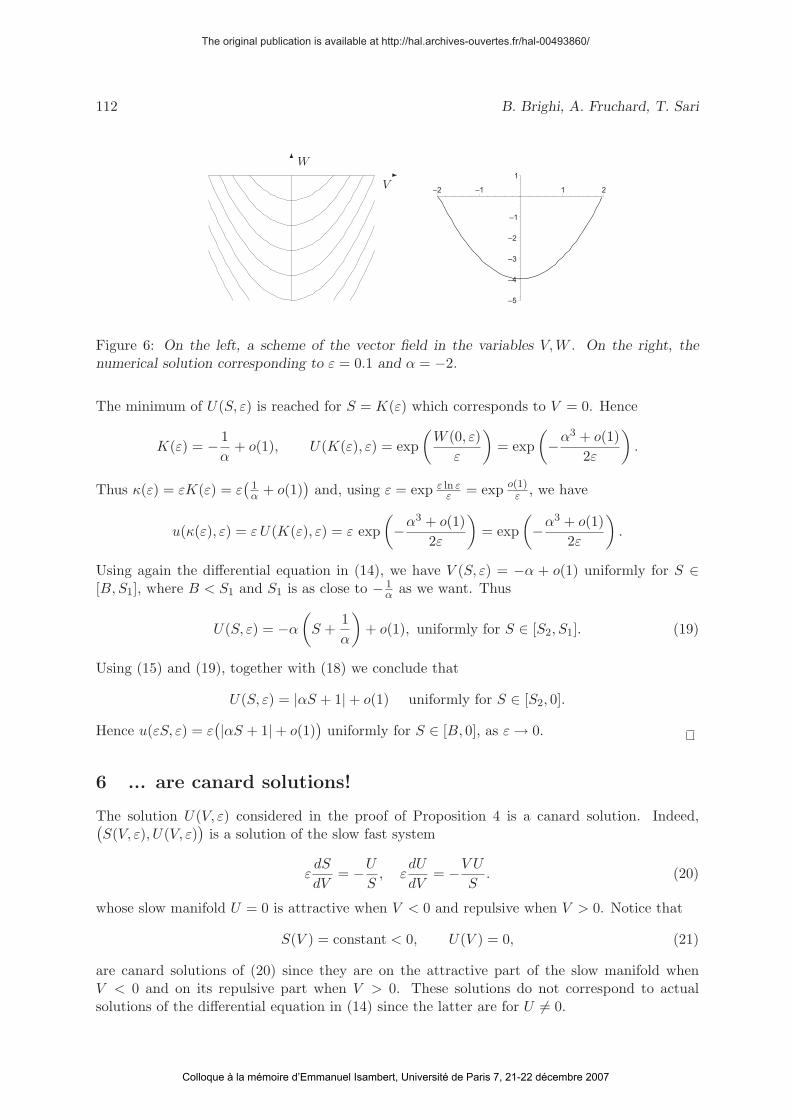
Figure 6: On the left, a scheme of the vector field in the variables V, W . On the right, thenumerical solution corresponding to ε = 0.1 and α = −2.

The minimum of U(S, ε) is reached for S = K(ε) which corresponds to V = 0. Hence

K(ε) = − 1

α+ o(1), U(K(ε), ε) = exp

(W (0, ε)

ε

)= exp

(−α3 + o(1)

2ε

).

Thus κ(ε) = εK(ε) = ε(

1α + o(1)

)and, using ε = exp ε ln ε

ε = exp o(1)ε , we have

u(κ(ε), ε) = εU(K(ε), ε) = ε exp

(−α3 + o(1)

2ε

)= exp

(−α3 + o(1)

2ε

).

Using again the differential equation in (14), we have V (S, ε) = −α + o(1) uniformly for S ∈[B, S1], where B < S1 and S1 is as close to − 1

α as we want. Thus

U(S, ε) = −α

(S +

1

α

)+ o(1), uniformly for S ∈ [S2, S1]. (19)

Using (15) and (19), together with (18) we conclude that

U(S, ε) = |αS + 1| + o(1) uniformly for S ∈ [S2, 0].

Hence u(εS, ε) = ε(|αS + 1| + o(1)

)uniformly for S ∈ [B, 0], as ε → 0.

6 ... are canard solutions!

The solution U(V, ε) considered in the proof of Proposition 4 is a canard solution. Indeed,(S(V, ε), U(V, ε)

)is a solution of the slow fast system

εdS

dV= −U

S, ε

dU

dV= −V U

S. (20)

whose slow manifold U = 0 is attractive when V < 0 and repulsive when V > 0. Notice that

S(V ) = constant < 0, U(V ) = 0, (21)

are canard solutions of (20) since they are on the attractive part of the slow manifold whenV < 0 and on its repulsive part when V > 0. These solutions do not correspond to actualsolutions of the differential equation in (14) since the latter are for U = 0.




�T

S

V

�(α,0,−1)

�

��(α,− 1

α,−1)

��(−α,− 1

α,1)

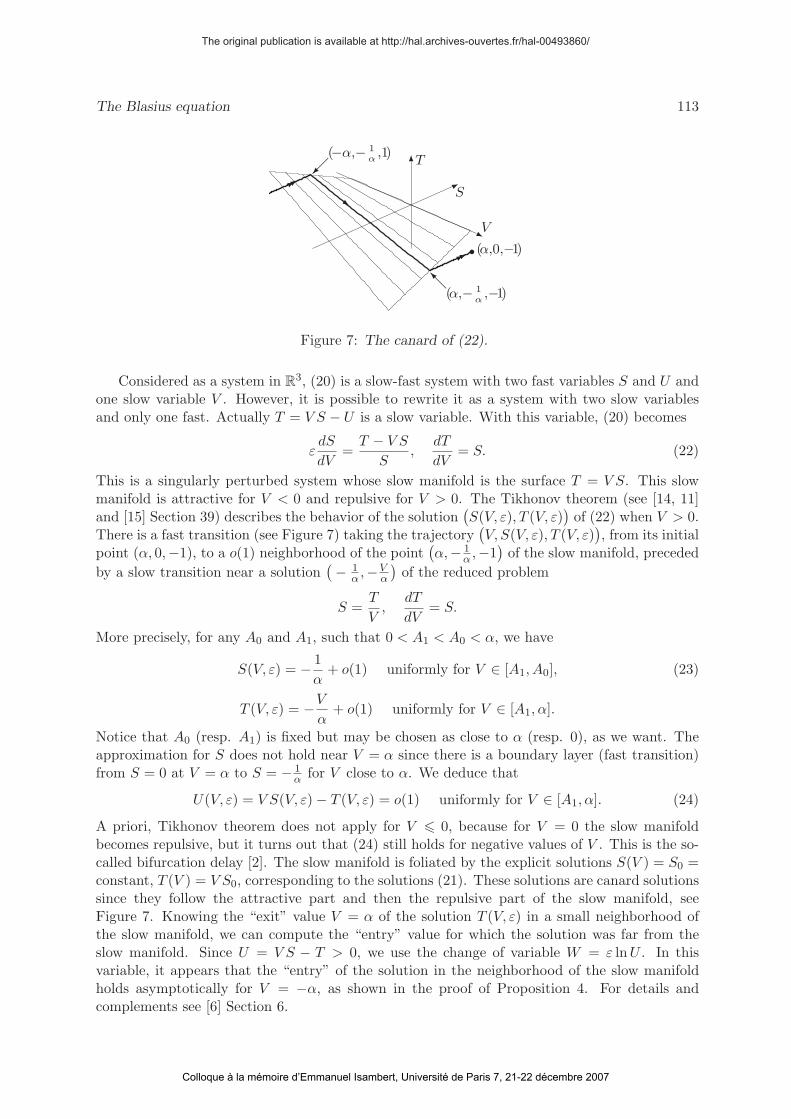
Figure 7: The canard of (22).

Considered as a system in R3, (20) is a slow-fast system with two fast variables S and U and

one slow variable V . However, it is possible to rewrite it as a system with two slow variablesand only one fast. Actually T = V S − U is a slow variable. With this variable, (20) becomes

εdS

dV=

T − V S

S,

dT

dV= S. (22)

This is a singularly perturbed system whose slow manifold is the surface T = V S. This slowmanifold is attractive for V < 0 and repulsive for V > 0. The Tikhonov theorem (see [14, 11]and [15] Section 39) describes the behavior of the solution

(S(V, ε), T (V, ε)

)of (22) when V > 0.

There is a fast transition (see Figure 7) taking the trajectory(V, S(V, ε), T (V, ε)

), from its initial

point (α, 0,−1), to a o(1) neighborhood of the point(α,− 1

α ,−1)

of the slow manifold, preceded

by a slow transition near a solution( − 1

α ,−Vα

)of the reduced problem

S =T

V,

dT

dV= S.

More precisely, for any A0 and A1, such that 0 < A1 < A0 < α, we have

S(V, ε) = − 1

α+ o(1) uniformly for V ∈ [A1, A0], (23)

T (V, ε) = −V

α+ o(1) uniformly for V ∈ [A1, α].

Notice that A0 (resp. A1) is fixed but may be chosen as close to α (resp. 0), as we want. Theapproximation for S does not hold near V = α since there is a boundary layer (fast transition)from S = 0 at V = α to S = − 1

α for V close to α. We deduce that

U(V, ε) = V S(V, ε) − T (V, ε) = o(1) uniformly for V ∈ [A1, α]. (24)

A priori, Tikhonov theorem does not apply for V � 0, because for V = 0 the slow manifoldbecomes repulsive, but it turns out that (24) still holds for negative values of V . This is the so-called bifurcation delay [2]. The slow manifold is foliated by the explicit solutions S(V ) = S0 =constant, T (V ) = V S0, corresponding to the solutions (21). These solutions are canard solutionssince they follow the attractive part and then the repulsive part of the slow manifold, seeFigure 7. Knowing the “exit” value V = α of the solution T (V, ε) in a small neighborhood ofthe slow manifold, we can compute the “entry” value for which the solution was far from theslow manifold. Since U = V S − T > 0, we use the change of variable W = ε lnU . In thisvariable, it appears that the “entry” of the solution in the neighborhood of the slow manifoldholds asymptotically for V = −α, as shown in the proof of Proposition 4. For details andcomplements see [6] Section 6.




7 The discontinuity of the function Λ

Two particular solutions of the Crocco equation (6) play an important role in our study.

0.2

0.4

0.6

0.8

1

1.2

1.4

0–1 –0.8 –0.6 –0.4 –0.2

0

0.2

0.4

0.2 0.4 0.6 0.8 1 1.2 1.4

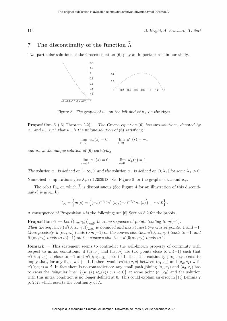
Figure 8: The graphs of u− on the left and of u+ on the right.

Proposition 5 ([6] Theorem 2.2) — The Crocco equation (6) has two solutions, denoted byu− and u+ such that u− is the unique solution of (6) satisfying

lims→0−

u−(s) = 0, lims→0−

u′−(s) = −1

and u+ is the unique solution of (6) satisfying

lims→0+

u+(s) = 0, lims→0+

u′+(s) = 1.

The solution u− is defined on ]−∞, 0[ and the solution u+ is defined on ]0, λ+[ for some λ+ > 0.

Numerical computations give λ+ ≈ 1.303918. See Figure 8 for the graphs of u− and u+.

The orbit Γ∞ on which Λ is discontinuous (See Figure 4 for an illustration of this disconti-nuity) is given by

Γ∞ ={

m(s) =((−s)−1/2u′

−(s), (−s)−3/2u−(s))

; s < 0}

.

A consequence of Proposition 4 is the following; see [6] Section 5.2 for the proofs.

Proposition 6 — Let((αn, γn)

)n∈N

be some sequence of points tending to m(−1).

Then the sequence(u′(0;αn, γn)

)n∈N

is bounded and has at most two cluster points: 1 and −1.More precisely, if (αn, γn) tends to m(−1) on the convex side then u′(0;αn, γn) tends to −1, andif (αn, γn) tends to m(−1) on the concave side then u′(0;αn, γn) tends to 1.

Remark — This statement seems to contradict the well-known property of continuity withrespect to initial conditions: if (a1, c1) and (a2, c2) are two points close to m(−1) such thatu′(0; a1, c1) is close to −1 and u′(0; a2, c2) close to 1, then this continuity property seems toimply that, for any fixed d ∈ ] − 1, 1[ there would exist (a, c) between (a1, c1) and (a2, c2) withu′(0; a, c) = d. In fact there is no contradiction: any small path joining (a1, c1) and (a2, c2) hasto cross the “singular line”

{(u−(s), u′

−(s))

; s < 0}

at some point (a0, c0) and the solutionwith this initial condition is no longer defined at 0. This could explain an error in [13] Lemma 2p. 257, which asserts the continuity of Λ.




8

2

6

0

4

2

-20

-4-6

1

0

-1

2

-2

-3

0-2-4-6

2

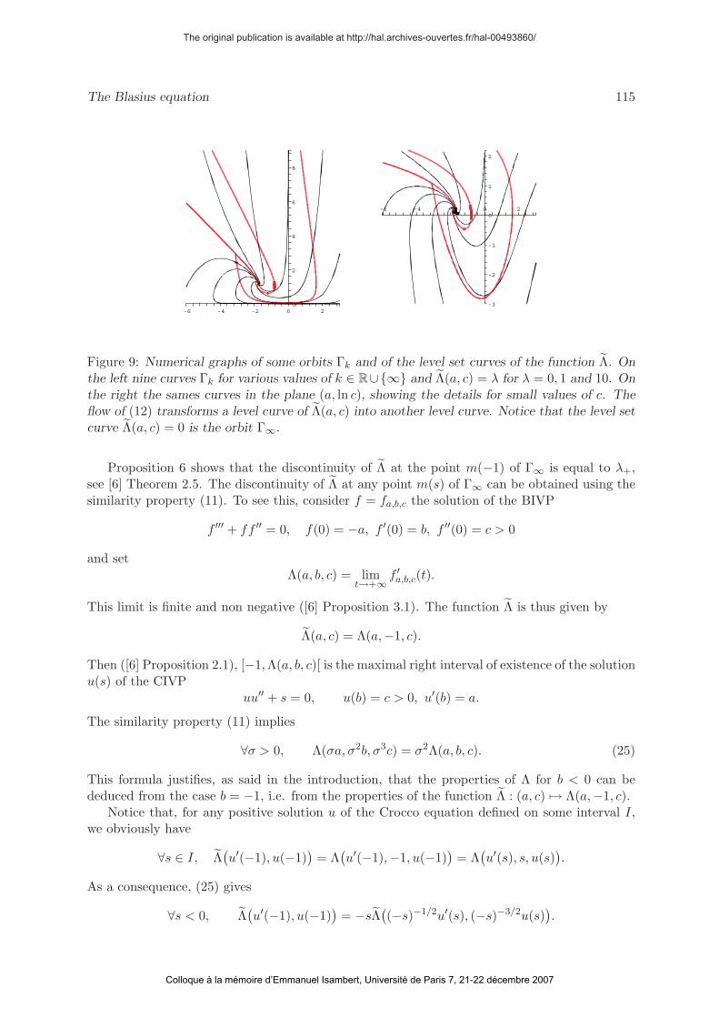
Figure 9: Numerical graphs of some orbits Γk and of the level set curves of the function Λ. Onthe left nine curves Γk for various values of k ∈ R∪{∞} and Λ(a, c) = λ for λ = 0, 1 and 10. Onthe right the sames curves in the plane (a, ln c), showing the details for small values of c. Theflow of (12) transforms a level curve of Λ(a, c) into another level curve. Notice that the level setcurve Λ(a, c) = 0 is the orbit Γ∞.

Proposition 6 shows that the discontinuity of Λ at the point m(−1) of Γ∞ is equal to λ+,see [6] Theorem 2.5. The discontinuity of Λ at any point m(s) of Γ∞ can be obtained using thesimilarity property (11). To see this, consider f = fa,b,c the solution of the BIVP

f ′′′ + ff ′′ = 0, f(0) = −a, f ′(0) = b, f ′′(0) = c > 0

and setΛ(a, b, c) = lim

t→+∞f ′

a,b,c(t).

This limit is finite and non negative ([6] Proposition 3.1). The function Λ is thus given by

Λ(a, c) = Λ(a,−1, c).

Then ([6] Proposition 2.1), [−1, Λ(a, b, c)[ is the maximal right interval of existence of the solutionu(s) of the CIVP

uu′′ + s = 0, u(b) = c > 0, u′(b) = a.

The similarity property (11) implies

∀σ > 0, Λ(σa, σ2b, σ3c) = σ2Λ(a, b, c). (25)

This formula justifies, as said in the introduction, that the properties of Λ for b < 0 can bededuced from the case b = −1, i.e. from the properties of the function Λ : (a, c) �→ Λ(a,−1, c).

Notice that, for any positive solution u of the Crocco equation defined on some interval I,we obviously have

∀s ∈ I, Λ(u′(−1), u(−1)

)= Λ

(u′(−1),−1, u(−1)

)= Λ

(u′(s), s, u(s)

).

As a consequence, (25) gives

∀s < 0, Λ(u′(−1), u(−1)

)= −sΛ

((−s)−1/2u′(s), (−s)−3/2u(s)

).




In terms of the associated vector field, we deduce that for all (x, y) solution of (12)

∀τ ∈ R, Λ(x(τ), y(τ)

)= eτ Λ

(x(0), y(0)

). (26)

This formula shows how the τ -map flow of (12) transforms the level curve Λ(a, c) = λ into thelevel curve Λ(a, c) = eτλ, see Figure 9. Hence the similarity property (11) yields the discontinuityat any point of Γ∞.

Corollary 7 — The discontinuity of Λ at a point m(s) of Γ∞ is as follows: on the convex sideof Γ∞, Λ tends to 0, whereas on the concave side, Λ tends to −λ+

s .

8 The number of solutions of the BBVP

To count the number of solutions of (5) we adopt the following strategy: for any values of a ∈ R

and λ � 0, we count the number of values of c for which Λ(a, c) = λ where Λ : R×]0, +∞[→[0, +∞[ is the limit defined by (9). Let A(λ) denote the abscissa of the point of Γ∞ where Λtakes the values 0 and λ on each side of Γ∞ respectively. Corollary 7 yields −s = λ+

λ , fromwhich we deduce that

A : ]0, +∞[ → ]−∞, 0[ , λ �→√

λλ+

u′−

(−λ+

λ

).

–3

–2

–1

01 2 3 4 5 6

–1.73

–1.725

–1.72

–1.715

0 0.02 0.04 0.06 0.08 0.1

−√3

a = A(λ)

λ

−√3

a

λ

a = A(λ)

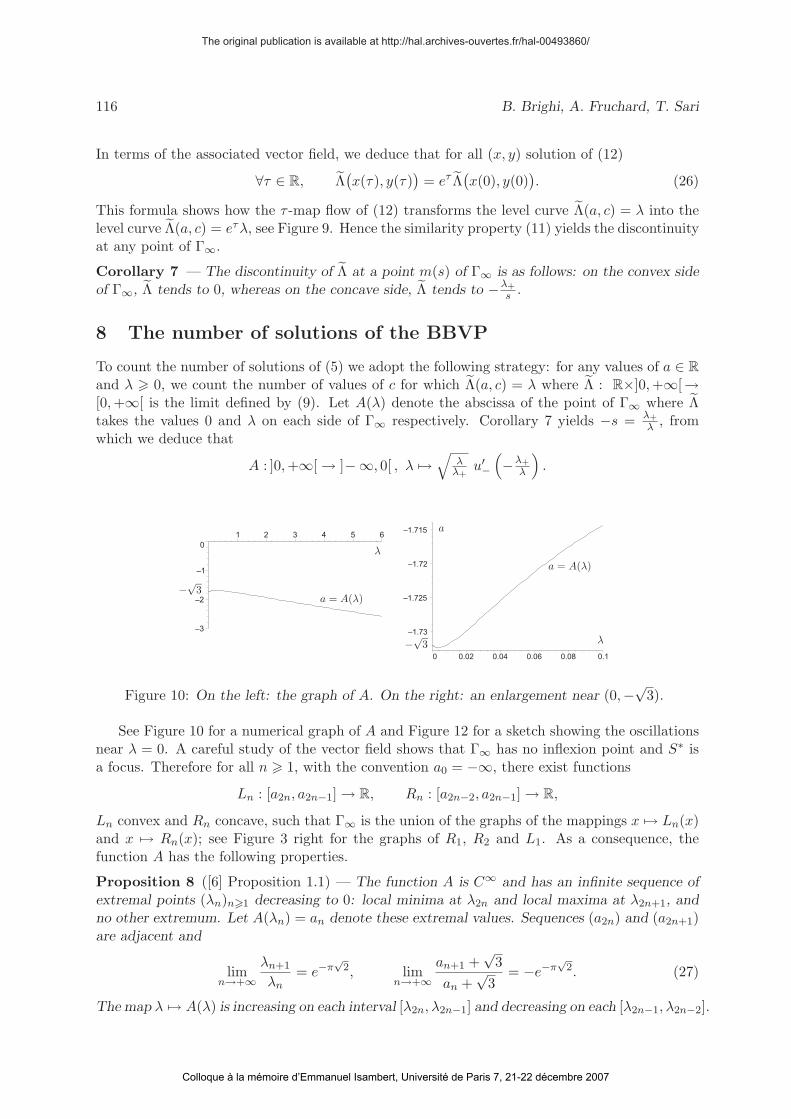
Figure 10: On the left: the graph of A. On the right: an enlargement near (0,−√3).

See Figure 10 for a numerical graph of A and Figure 12 for a sketch showing the oscillationsnear λ = 0. A careful study of the vector field shows that Γ∞ has no inflexion point and S∗ isa focus. Therefore for all n � 1, with the convention a0 = −∞, there exist functions

Ln : [a2n, a2n−1] → R, Rn : [a2n−2, a2n−1] → R,

Ln convex and Rn concave, such that Γ∞ is the union of the graphs of the mappings x �→ Ln(x)and x �→ Rn(x); see Figure 3 right for the graphs of R1, R2 and L1. As a consequence, thefunction A has the following properties.

Proposition 8 ([6] Proposition 1.1) — The function A is C∞ and has an infinite sequence ofextremal points (λn)n�1 decreasing to 0: local minima at λ2n and local maxima at λ2n+1, andno other extremum. Let A(λn) = an denote these extremal values. Sequences (a2n) and (a2n+1)are adjacent and

limn→+∞

λn+1

λn= e−π

√2, lim

n→+∞an+1 +

√3

an +√

3= −e−π

√2. (27)

The map λ �→ A(λ) is increasing on each interval [λ2n, λ2n−1] and decreasing on each [λ2n−1, λ2n−2].




Hence for all n � 1, with the convention λ0 = +∞, there exist one-to-one mappings

ln : [a2n, a2n−1] → [λ2n, λ2n−1], rn : [a2n−2, a2n−1] → [λ2n−1, λ2n−2],

such that the graph of λ �→ A(λ) is the union of the graphs of a �→ ln(a) and a �→ rn(a), seeFigure 12 left for the graphs of r1, r2 and l1.

Given a ∈ R and λ � 0, counting the number of solutions of the Blasius Problem (1 - 5)amounts to counting the number of times the function Λ takes the value λ on a vertical ray

Da := {a}×]0,+∞[. (28)

For that purpose, we introduce the function

Λa : ]0, +∞[→ [0, +∞[, c �→ Λ(a, c).

The description below is succinct. We refer to [6] Section 2.4 for proofs, additional details andexplanatory figures.

Let n � 1 be such that a is between an−2 and an, possibly a = an (with the conventiona−1 = +∞, a0 = −∞). Then the ray Da crosses n − 1 times the spiral Γ∞ (if a = an, thereis an n-th point of contact but without crossing, hence without creating any discontinuity forΛa). To fix ideas, assume that n is odd. A similar description can be done for n even. Then the

�λ

�c0

�

)

L1(a)

l1(a)

�

R1(a)

r1(a) (

C3(a)Λ3(a)

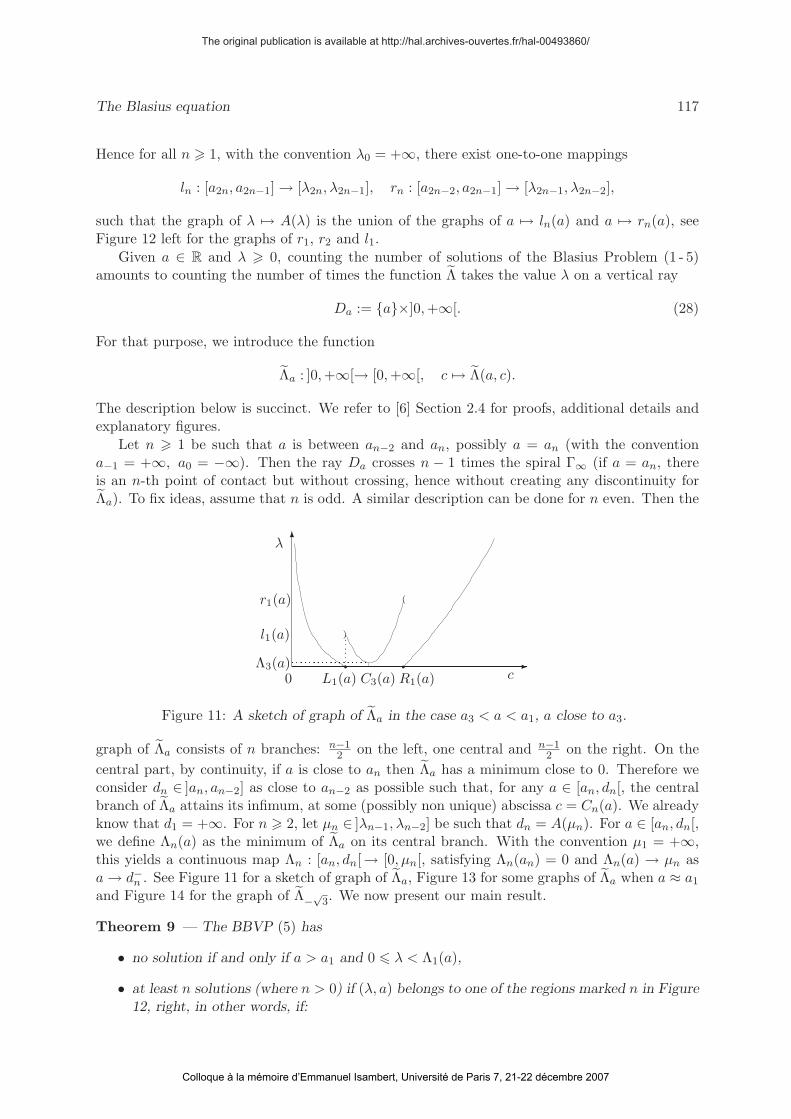
Figure 11: A sketch of graph of Λa in the case a3 < a < a1, a close to a3.

graph of Λa consists of n branches: n−12 on the left, one central and n−1

2 on the right. On the

central part, by continuity, if a is close to an then Λa has a minimum close to 0. Therefore weconsider dn ∈ ]an, an−2] as close to an−2 as possible such that, for any a ∈ [an, dn[, the centralbranch of Λa attains its infimum, at some (possibly non unique) abscissa c = Cn(a). We alreadyknow that d1 = +∞. For n � 2, let μn ∈ ]λn−1, λn−2] be such that dn = A(μn). For a ∈ [an, dn[,we define Λn(a) as the minimum of Λa on its central branch. With the convention μ1 = +∞,this yields a continuous map Λn : [an, dn[→ [0, μn[, satisfying Λn(an) = 0 and Λn(a) → μn asa → d−n . See Figure 11 for a sketch of graph of Λa, Figure 13 for some graphs of Λa when a ≈ a1

and Figure 14 for the graph of Λ−√

3. We now present our main result.

Theorem 9 — The BBVP (5) has

• no solution if and only if a > a1 and 0 � λ < Λ1(a),

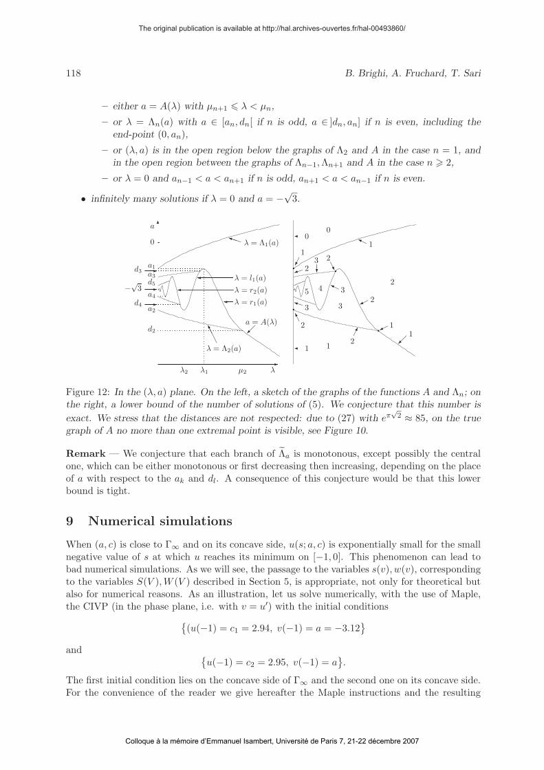
• at least n solutions (where n > 0) if (λ, a) belongs to one of the regions marked n in Figure12, right, in other words, if:




– either a = A(λ) with μn+1 � λ < μn,

– or λ = Λn(a) with a ∈ [an, dn[ if n is odd, a ∈ ]dn, an] if n is even, including theend-point (0, an),

– or (λ, a) is in the open region below the graphs of Λ2 and A in the case n = 1, andin the open region between the graphs of Λn−1, Λn+1 and A in the case n � 2,

– or λ = 0 and an−1 < a < an+1 if n is odd, an+1 < a < an−1 if n is even.

• infinitely many solutions if λ = 0 and a = −√3.

�a

0

a1�d3 a3

d5�−√3

a4

�d4a2

d2

�λμ2λ1λ2

��

λ = Λ2(a)

��λ = Λ1(a)

� λ = r1(a)

� λ = l1(a)� λ = r2(a)

��a = A(λ)

0

2

1

3

45

� 0

�3��

1

�� 2

��3

� 2

�

� 1

�� 1

�� 2

�� 1�

�� 3

��2

�

��2 ��

1

Figure 12: In the (λ, a) plane. On the left, a sketch of the graphs of the functions A and Λn; onthe right, a lower bound of the number of solutions of (5). We conjecture that this number is

exact. We stress that the distances are not respected: due to (27) with eπ√

2 ≈ 85, on the truegraph of A no more than one extremal point is visible, see Figure 10.

Remark — We conjecture that each branch of Λa is monotonous, except possibly the centralone, which can be either monotonous or first decreasing then increasing, depending on the placeof a with respect to the ak and dl. A consequence of this conjecture would be that this lowerbound is tight.

9 Numerical simulations

When (a, c) is close to Γ∞ and on its concave side, u(s; a, c) is exponentially small for the smallnegative value of s at which u reaches its minimum on [−1, 0]. This phenomenon can lead tobad numerical simulations. As we will see, the passage to the variables s(v), w(v), correspondingto the variables S(V ), W (V ) described in Section 5, is appropriate, not only for theoretical butalso for numerical reasons. As an illustration, let us solve numerically, with the use of Maple,the CIVP (in the phase plane, i.e. with v = u′) with the initial conditions{

(u(−1) = c1 = 2.94, v(−1) = a = −3.12}

and {u(−1) = c2 = 2.95, v(−1) = a

}.

The first initial condition lies on the concave side of Γ∞ and the second one on its concave side.For the convenience of the reader we give hereafter the Maple instructions and the resulting




0

0.1

0.2

0.3

0.4

1 1.1 1.2 1.3 1.4 1.5 0

0.1

0.2

0.3

0.4

1 1.1 1.2 1.3 1.4 1.5

0

0.1

0.2

0.3

0.4

1 1.1 1.2 1.3 1.4 1.5 0

0.1

0.2

0.3

0.4

1 1.1 1.2 1.3 1.4 1.5

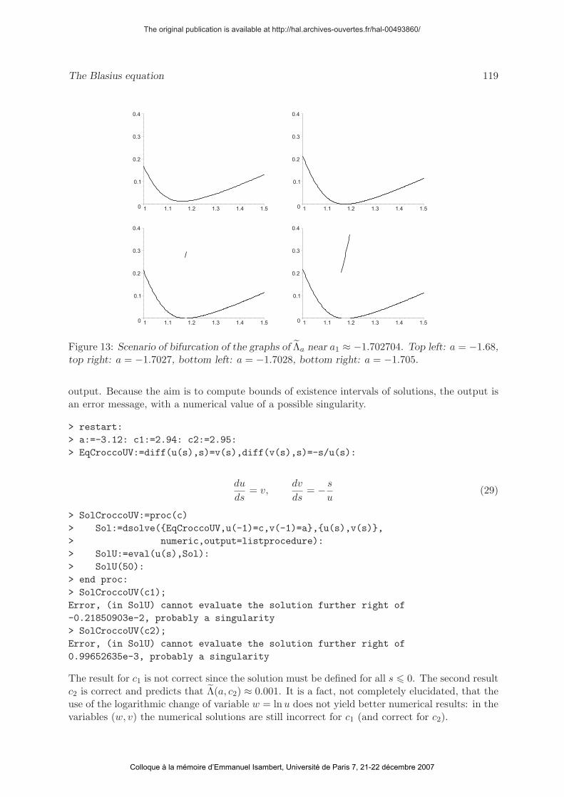
Figure 13: Scenario of bifurcation of the graphs of Λa near a1 ≈ −1.702704. Top left: a = −1.68,top right: a = −1.7027, bottom left: a = −1.7028, bottom right: a = −1.705.

output. Because the aim is to compute bounds of existence intervals of solutions, the output isan error message, with a numerical value of a possible singularity.

> restart:

> a:=-3.12: c1:=2.94: c2:=2.95:

> EqCroccoUV:=diff(u(s),s)=v(s),diff(v(s),s)=-s/u(s):

du

ds= v,

dv

ds= − s

u(29)

> SolCroccoUV:=proc(c)

> Sol:=dsolve({EqCroccoUV,u(-1)=c,v(-1)=a},{u(s),v(s)},

> numeric,output=listprocedure):

> SolU:=eval(u(s),Sol):

> SolU(50):

> end proc:

> SolCroccoUV(c1);

Error, (in SolU) cannot evaluate the solution further right of

-0.21850903e-2, probably a singularity

> SolCroccoUV(c2);

Error, (in SolU) cannot evaluate the solution further right of

0.99652635e-3, probably a singularity

The result for c1 is not correct since the solution must be defined for all s � 0. The second resultc2 is correct and predicts that Λ(a, c2) ≈ 0.001. It is a fact, not completely elucidated, that theuse of the logarithmic change of variable w = lnu does not yield better numerical results: in thevariables (w, v) the numerical solutions are still incorrect for c1 (and correct for c2).




0

2

4

6

8

10

0.5 1 1.5 2 2.5 3 3.5 4 0

0.2

0.4

0.6

0.8

1 1.1 1.2 1.3 1.4 1.5

0

0.005

0.01

0.015

0.02

1.152 1.154 1.156 1.158 1.16 0

2e–05

4e–05

6e–05

8e–05

0.0001

0.00012

1.15466 1.1547 1.15472 1.15474 1.15476

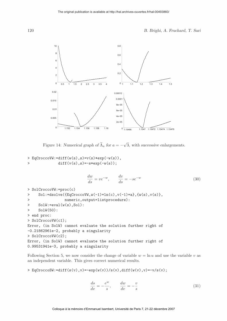
Figure 14: Numerical graph of Λa for a = −√3, with successive enlargements.

> EqCroccoVW:=diff(w(s),s)=v(s)*exp(-w(s)),

> diff(v(s),s)=-s*exp(-w(s));

dw

ds= ve−w,

dv

ds= −se−w (30)

> SolCroccoVW:=proc(c)

> Sol:=dsolve({EqCroccoVW,w(-1)=ln(c),v(-1)=a},{w(s),v(s)},


> SolW:=eval(w(s),Sol):

> SolW(50):

> end proc:

> SolCroccoVW(c1);

Error, (in SolW) cannot evaluate the solution further right of

-0.21862961e-2, probably a singularity

> SolCroccoVW(c2);

Error, (in SolW) cannot evaluate the solution further right of

0.99531941e-3, probably a singularity

Following Section 5, we now consider the change of variable w = lnu and use the variable v asan independent variable. This gives correct numerical results.

> EqCroccoSW:=diff(s(v),v)=-exp(w(v))/s(v),diff(w(v),v)=-v/s(v);

ds

dv= −ew

s,

dw

dv= −v

s(31)




> SolCroccoSW:=proc(c)

> Sol:=dsolve({EqCroccoSW,w(a)=ln(c),s(a)=-1},{w(v),s(v)},


> SolS:=eval(s(v),Sol):

> SolS(10):

> end proc:

> SolCroccoSW(c1);

Error, (in SolS) cannot evaluate the solution further right of

2.7651840, probably a singularity

> SolCroccoSW(c2);

Error, (in SolS) cannot evaluate the solution further right of

-2.7726621, probably a singularity

We see that for c1, the solution w(v) is computed until the value v = 2.7651840. Hence thenumerical solution succeeded to pass exponentially close to the axis u = 0 and to reflect on thisaxis and get a positive derivative. The singularity encountered now at v = 2.7651840 is causedby the fact that system (31) is defined only in the half space s < 0. For s � 0 we must return tothe original variables u(s) and v(s). Hence we use the following procedure to evaluate Λ(a, c).

> Lambda:= proc(a,c)

> erreur:=0.0000000001:

> fSW:=dsolve({EqCroccoSW,w(a)=ln(c),s(a)=-1},{s(v),w(v)},

> numeric,stop_cond=[s(v)+erreur]):

> fSW(10);

> IC:=subs(%,[v,s(v),w(v)]):

> v0:=IC[1]: s0:=IC[2]: w0:=IC[3]:

> f:=dsolve({EqCroccoUV,u(s0)=exp(w0),v(s0)=v0},{u(s),v(s)},

> numeric,stop_cond=[u(s)-erreur]):

> f(50):

> subs(%,s):

> end proc:

This procedure is easy to understand. First system (31) is solved with initial conditions w(a) =ln(c), s(a) = −1 as far as s � −erreur. Next, one computes the values v0, s0 = s(v0) andw0 = w(v0) such that the stopping condition s0 = −erreur is reached. Then system (29) issolved with initial conditions u(s0) = ew0 , v(s0) = v0, as far as u � erreur. The proceduregives the value s1 such that the stopping condition u(s1) = erreur is attained. This value is avery good approximation of Λ(a, c).

> Lambda(a,c1);

Warning, cannot evaluate the solution further right of

2.7651840, stop condition #1 violated


10.012058, stop condition #1 violated

10.0120586420604791

> Lambda(a,c2);


-2.7726621, stop condition #1 violated


.99606109e-3, stop condition #1 violated




0.000996061092810659674

Hence, Λ(a, c1) ≈ 10.012 and Λ(a, c2) ≈ 0.001. The following instructions which use the proce-dure Lambda produce the numerical graph of Λa for a = −√

3 and 1.15466 � c � 1.15476, seeFigure 14 bottom right.

> a:=-sqrt(3): c1:=1.15466: c2:=1.15476: N:=200;

> for n from 0 to N do LLambda[n]:=c1+n*(c2-c1)/N,

> Lambda(a,c1+n*(c2-c1)/N) end do:

> L1:=[[LLambda[i]]$i=0..112]: L2:=[[LLambda[i]]$i=113..N]:

> plot([L1,L2],c1..c2,-.0000031..0.00012,thickness =4,

> color=black);

References

[1] Z. Belhachmi, B. Brighi K. Taous, On the concave solutions of the Blasius equation, Acta

Math. Univ. Comenianae 69:2 (2000) 199-214.

[2] E. Benoıt Ed., Dynamic Bifurcations, Proceedings Luminy 1990, Lect. Notes Math. 1493Springer-Verlag, 1991.

[3] H. Blasius, Thesis, Gottingen (1907).

[4] H. Blasius, Grenzschichten in Flussigkeiten mit kleiner Reibung, Zeitschr. Math. Phys. 56(1908) 1-37.

[5] B. Brighi, Deux problemes aux limites pour l’equation de Blasius, Revue Math. Ens. Sup.

8 (2001) 833-842.

[6] B. Brighi, A. Fruchard T. Sari, On the Blasius Problem, Adv. Differential Equations 13,no. 5-6 (2008) 509–600.

[7] L. Crocco, Sull strato limite laminare nei gas lungo una lamina plana, Rend. Math. Appl.

Ser. 5 21 (1941) 138-152.

[8] P. Hartman, Ordinary Differential Equations, Wiley, 1964.

[9] M. Y. Hussaini W. D. Laikin, Existence and non-uniqueness of similarity solutions of aboundary layer problem, Quart. J. Mech. Appl. Math. 39:1 (1986) 15-24.

[10] M. Y. Hussaini, W. D. Laikin A. Nachman, On similarity solutions of a boundary layerproblem with an upstream moving wall, SIAM J. Appl. Math. 47:4 (1987) 699-709.

[11] C. Lobry, T. Sari S. Touhami, On Tykhonov’s theorem for convergence of solutions of slowand fast systems, Electron. J. Differential Equations 19 (1998) 1-22.

[12] O. A. Oleinik, V. N. Samokhin, Mathematical Models in Boundary Layer Theory, Ap-plied Mathematics and Mathematical Computations 15, Chapman& Hall/CRC, Washing-ton, 1999.

[13] E. Soewono, K. Vajravelu R.N. Mohapatra, Existence and nonuniqueness of solutions of asingular non linear boundary layer problem, J. Math. Anal. Appl. 159 (1991) 251-270.




[14] A. N. Tikhonov, Systems of differential equations containing small parameters multiplyingthe derivatives, Mat. Sb. 31 (1952) 575-586.

[15] W. Wasow, Asymptotic Expansions for Ordinary Differential Equations, Krieger, New York,1976.

[16] H. Weyl, On the differential equations of the simplest boundary-layer problems, Ann. Math.

43 (1942) 381-407.

Address of the authors:

Laboratoire de Mathematiques, Informatique et Applications, EA3993Faculte des Sciences et Techniques, Universite de Haute Alsace4, rue des Freres Lumiere, F-68093 Mulhouse cedex, France

Current address for T. Sari:

UMR ITAP, CEMAGREF, Domaine de Lavalette361, rue J.-F. Breton, BP 5095F-34196 Montpellier Cedex 5, France

E-addresses:

[email protected]

[email protected]

[email protected]






Date post:	12-Feb-2022
Category:	Documents
Upload:	others
View:	11 times
Download:	0 times

The Blasius equation - HAL - INRIA

Documents